Temporal scale selection in time-causal scale space††thanks: The support from the Swedish Research Council (Contract No. 2014-4083) and Stiftelsen Olle Engkvist Byggmästare (Contract No. 2015/465) is gratefully acknowledged.
Abstract
When designing and developing scale selection mechanisms for generating hypotheses about characteristic scales in signals, it is essential that the selected scale levels reflect the extent of the underlying structures in the signal.
This paper presents a theory and in-depth theoretical analysis about the scale selection properties of methods for automatically selecting local temporal scales in time-dependent signals based on local extrema over temporal scales of scale-normalized temporal derivative responses. Specifically, this paper develops a novel theoretical framework for performing such temporal scale selection over a time-causal and time-recursive temporal domain as is necessary when processing continuous video or audio streams in real time or when modelling biological perception.
For a recently developed time-causal and time-recursive scale-space concept defined by convolution with a scale-invariant limit kernel, we show that it is possible to transfer a large number of the desirable scale selection properties that hold for the Gaussian scale-space concept over a non-causal temporal domain to this temporal scale-space concept over a truly time-causal domain. Specifically, we show that for this temporal scale-space concept, it is possible to achieve true temporal scale invariance although the temporal scale levels have to be discrete, which is a novel theoretical construction.
The analysis starts from a detailed comparison of different temporal scale-space concepts and their relative advantages and disadvantages, leading the focus to a class of recently extended time-causal and time-recursive temporal scale-space concepts based on first-order integrators or equivalently truncated exponential kernels coupled in cascade. Specifically, by the discrete nature of the temporal scale levels in this class of time-causal scale-space concepts, we study two special cases of distributing the intermediate temporal scale levels, by using either a uniform distribution in terms of the variance of the composed temporal scale-space kernel or a logarithmic distribution.
In the case of a uniform distribution of the temporal scale levels, we show that scale selection based on local extrema of scale-normalized derivatives over temporal scales makes it possible to estimate the temporal duration of sparse local features defined in terms of temporal extrema of first- or second-order temporal derivative responses. For dense features modelled as a sine wave, the lack of temporal scale invariance does, however, constitute a major limitation for handling dense temporal structures of different temporal duration in a uniform manner.
In the case of a logarithmic distribution of the temporal scale levels, specifically taken to the limit of a time-causal limit kernel with an infinitely dense distribution of the temporal scale levels towards zero temporal scale, we show that it is possible to achieve true temporal scale invariance to handle dense features modelled as a sine wave in a uniform manner over different temporal durations of the temporal structures as well to achieve more general temporal scale invariance for any signal over any temporal scaling transformation with a scaling factor that is an integer power of the distribution parameter of the time-causal limit kernel.
It is shown how these temporal scale selection properties developed for a pure temporal domain carry over to feature detectors defined over time-causal spatio-temporal and spectro-temporal domains.
Keywords:
Scale space Scale Scale selection Temporal Spatio-temporal Scale invariance Differential invariant Feature detection Video analysis Computer vision1 Introduction
When processing sensory data by automatic methods in areas of signal processing such as computer vision or audio processing or in computational modelling of biological perception, the notion of receptive field constitutes an essential concept (Hubel and Wiesel HubWie59-Phys ; HubWie05-book ; Aertsen and Johannesma AerJoh81-BICY ; DeAngelis et al. DeAngOhzFre95-TINS ; deAngAnz04-VisNeuroSci ; Miller et al MilEscReaSch01-JNeuroPhys ).
For sensory data as obtained from vision or hearing, or their counterparts in artificial perception, the measurement from a single light sensor in a video camera or on the retina, or the instantaneous sound pressure registered by a microphone is hardly meaningful at all, since any such measurement is strongly dependent on external factors such as the illumination of a visual scene regarding vision or the distance between the sound source and the microphone regarding hearing. Instead, the essential information is carried by the relative relations between local measurements at different points and temporal moments regarding vision or local measurements over different frequencies and temporal moments regarding hearing. Following this paradigm, sensory measurements should be performed over local neighbourhoods over space-time regarding vision and over local neighbourhoods in the time-frequency domain regarding hearing, leading to the notions of spatio-temporal and spectro-temporal receptive fields.
Specifically, spatio-temporal receptive fields constitute a main class of primitives for expressing methods for video analysis (Zelnik-Manor and Irani ZelIra01-CVPR , Laptev and Lindeberg LapLin04-ECCVWS ; LapCapSchLin07-CVIU ; Jhuang et al. JhuSerWolPog07-ICCV ; Kläser et al. KlaMarSch08-BMVC ; Niebles et al. NieWanFei08-IJCV ; Wang et al. WanUllKlaLapSch09-BMVC ; Poppe et al. Pop09-IVC ; Shao and Mattivi ShaMatt10-CIVR ; Weinland et al. WeiRonBoy11-CVIU ; Wang et al. WanQiaTan15-CVPR ), whereas spectro-temporal receptive fields constitute a main class of primitives for expressing methods for machine hearing (Patterson et al. PatRobHolMcKeoZhaAll92-AudPhysPerc ; PatAllGig95-JASA ; Kleinschmidt Kle02-ActAcust ; Ezzat et al. EzzBouPog07-InterSpeech ; Meyer and Kollmeier MeyKol08-InterSpeech ; Schlute et al. SchBezWagNey07-ICASSP ; Heckmann et al. HecDomJouGoe11-SpeechComm ; Wu et al. WuZhaShi11-ASLP ; Alias et al. AliSocJoaSev16-ApplSci ).
A general problem when applying the notion of receptive fields in practice, however, is that the types of responses that are obtained in a specific situation can be strongly dependent on the scale levels at which they are computed. A spatio-temporal receptive field is determined by at least a spatial scale parameter and a temporal scale parameter, whereas a spectro-temporal receptive field is determined by at least a spectral and a temporal scale parameter. Beyond ensuring that local sensory measurements at different spatial, temporal and spectral scales are treated in a consistent manner, which by itself provides strong contraints on the shapes of the receptive fields (Lindeberg Lin13-BICY ; Lin16-JMIV ; Lindeberg and Friberg LinFri15-PONE ; LinFri15-SSVM ), it is necessary for computer vision or machine hearing algorithms to decide what responses within the families of receptive fields over different spatial, temporal and spectral scales they should base their analysis on.
Over the spatial domain, theoretically well-founded methods have been developed for choosing spatial scale levels among receptive field responses over multiple spatial scales (Lindeberg Lin97-IJCV ; Lin98-IJCV ; Lin99-CVHB ; Lin12-JMIV ; Lin14-EncCompVis ) leading to e.g. robust methods for image-based matching and recognition (Lowe Low04-IJCV ; Mikolajczyk and Schmid MikSch04-IJCV ; Tuytelaars and van Gool TuyGoo04-IJCV ; Bay et al. BayEssTuyGoo08-CVIU ; Tuytelaars and Mikolajczyk TuyMik08-Book ; van de Sande et al. SanGevSno10-PAMI ; Larsen et al. LarDarDahPed12-ECCV ) that are able to handle large variations of the size of the objects in the image domain and with numerous applications regarding object recognition, object categorization, multi-view geometry, construction of 3-D models from visual input, human-computer interaction, biometrics and robotics.
Much less research has, however, been performed regarding the topic of choosing local appropriate scales in temporal data. While some methods for temporal scale selection have been developed (Lindeberg Lin97-AFPAC ; Laptev and Lindeberg LapLin03-ICCV ; Willems et al. WilTuyGoo08-ECCV ), these methods suffer from either theoretical or practical limitations.
A main subject of this paper is present a theory for how to compare filter responses in terms of temporal derivatives that have been computed at different temporal scales, specifically with a detailed theoretical analysis of the possibilities of having temporal scale estimates as obtained from a temporal scale selection mechanism reflect the temporal duration of the underlying temporal structures that gave rise to the feature responses. Another main subject of this paper is to present a theoretical framework for temporal scale selection that leads to temporal scale invariance and enables the computation of scale covariant temporal scale estimates. While these topics can for a non-causal temporal domain be addressed by the non-causal Gaussian scale-space concept (Iijima Iij62 ; Witkin Wit83 ; Koenderink Koe84-BC ; Koenderink and van Doorn KoeDoo92-PAMI ; Lindeberg Lin93-Dis ; Lin94-SI ; Lin10-JMIV ; Florack Flo97-book ; ter Haar Romeny Haa04-book ), the development of such a theory has been missing regarding a time-causal temporal domain.
1.1 Temporal scale selection
When processing time-dependent signals in video or audio or more generally any temporal signal, special attention has to be put to the facts that:
-
•
the physical phenomena that generate the temporal signals may occur at different speed — faster or slower, and
-
•
the temporal signals may contain qualitatively different types of temporal structures at different temporal scales.
In certain controlled situations where the physical system that generates the temporal signals that is to be processed is sufficiently well known and if the variability of the temporal scales over time in the domain is sufficiently constrained, suitable temporal scales for processing the signals may in some situations be chosen manually and then be verified experimentally. If the sources that generate the temporal signals are sufficiently complex and/or if the temporal structures in the signals vary substantially in temporal duration by the underlying physical processes occurring significantly faster or slower, it is on the other hand natural to (i) include a mechanism for processing the temporal data at multiple temporal scales and (ii) try to detect in a bottom-up manner at what temporal scales the interesting temporal phenomena are likely to occur.
The subject of this article is to develop a theory for temporal scale selection in a time-causal temporal scale space as an extension of a previously developed theory for spatial scale selection in a spatial scale space (Lindeberg Lin97-IJCV ; Lin98-IJCV ; Lin99-CVHB ; Lin12-JMIV ; Lin14-EncCompVis ), to generate bottom-up hypotheses about characteristic temporal scales in time-dependent signals, intended to serve as estimates of the temporal duration of local temporal structures in time-dependent signals. Special focus will be on developing mechanisms analogous to scale selection in non-causal Gaussian scale-space, based on local extrema over scales of scale-normalized derivatives, while expressed within the framework of a time-causal and time-recursive temporal scale space in which the future cannot be accessed and the signal processing operations are thereby only allowed to make use of information from the present moment and a compact buffer of what has occurred in the past.
When designing and developing such scale selection mechanisms, it is essential that the computed scale estimates reflect the temporal duration of the corresponding temporal structures that gave rise to the feature responses. To understand the pre-requisites for developing such temporal scale selection methods, we will in this paper perform an in-depth theoretical analysis of the scale selection properties that such temporal scale selection mechanisms give rise to for different temporal scale-space concepts and for different ways of defining scale-normalized temporal derivatives.
Specifically, after an examination of the theoretical properties of different types of temporal scale-space concepts, we will focus on a class of recently extended time-causal temporal scale-space concepts obtained by convolution with truncated exponential kernels coupled in cascade (Lindeberg Lin90-PAMI ; Lin15-SSVM ; Lin16-JMIV ; Lindeberg and Fagerström LF96-ECCV ). For two natural ways of distributing the discrete temporal scale levels in such a representation, in terms of either a uniform distribution over the scale parameter corresponding to the variance of the composed scale-space kernel or a logarithmic distribution, we will study the scale selection properties that result from detecting local temporal scale levels from local extrema over scale of scale-normalized temporal derivatives. The motivation for studying a logarithmic distribution of the temporal scale levels, is that it corresponds to a uniform distribution in units of effective scale for some constants and , which has been shown to constitute the natural metric for measuring the scale levels in a spatial scale space (Koenderink Koe84-BC ; Lindeberg Lin92-PAMI ).
As we shall see from the detailed theoretical analysis that will follow, this will imply certain differences in scale selection properties of a temporally asymmetric time-causal scale space compared to scale selection in a spatially mirror symmetric Gaussian scale space. These differences in theoretical properties are in turn essential to take into explicit account when formulating algorithms for temporal scale selection in e.g. video analysis or audio analysis applications.
For the temporal scale-space concept based on a uniform distribution of the temporal scale levels in units of the variance of the composed scale-space kernel, it will be shown that temporal scale selection from local extrema over temporal scales will make it possible to estimate the temporal duration of local temporal structures modelled as local temporal peaks and local temporal ramps. For a dense temporal structure modelled as a temporal sine wave, the lack of true scale invariance for this concept will, however, imply that the temporal scale estimates will not be directly proportional to the wavelength of the temporal sine wave. Instead, the scale estimates are affected by a bias, which is not a desirable property.
For the temporal scale-space concept based on a logarithmic distribution of the temporal scale levels, and taken to the limit to scale-invariant time-causal limit kernel (Lindeberg Lin16-JMIV ) corresponding to an infinite number of temporal scale levels that cluster infinitely close near the temporal scale level zero, it will on the other hand be shown that the temporal scale estimates of a dense temporal sine wave will be truly proportional to the wavelength of the signal. By a general proof, it will be shown this scale invariant property of temporal scale estimates can also be extended to any sufficiently regular signal, which constitutes a general foundation for expressing scale invariant temporal scale selection mechanisms for time-dependent video and audio and more generally also other classes of time-dependent measurement signals.
As complement to this proposed overall framework for temporal scale selection, we will also present a set of general theoretical results regarding time-causal scale-space representations: (i) showing that previous application of the assumption of a semi-group property for time-causal scale-space concepts leads to undesirable temporal dynamics, which however can be remedied by replacing the assumption of a semi-group structure be a weaker assumption of a cascade property in turn based on a transitivity property, (ii) formulations of scale-normalized temporal derivatives for Koenderink’s time-causal scale-time model Koe88-BC and (iii) ways of translating the temporal scale estimates from local extrema over temporal scales in the temporal scale-space representation based on the scale-invariant time-causal limit kernel into quantitative measures of the temporal duration of the corresponding underlying temporal structures and in turn based on a scale-time approximation of the limit kernel.
In these ways, this paper is intended to provide a theoretical foundation for expressing theoretically well-founded temporal scale selection methods for selecting local temporal scales over time-causal temporal domains, such as video and audio with specific focus on real-time image or sound streams. Applications of this scale selection methodology for detecting both sparse and dense spatio-temporal features in video are presented in a companion paper Lin16-spattempscsel .
1.2 Structure of this article
As a conceptual background to the theoretical developments that will be performed, we will start in Section 2 with an overview of different approaches to handling temporal data within the scale-space framework including a comparison of relative advantages and disadvantages of different types of temporal scale-space concepts.
As a theoretical baseline for the later developments of methods for temporal scale selection in a time-causal scale space, we shall then in Section 3 give an overall description of basic temporal scale selection properties that will hold if the non-causal Gaussian scale-space concept with its corresponding selection methodology for a spatial image domain is applied to a one-dimensional non-causal temporal domain, e.g. for the purpose of handling the temporal domain when analysing pre-recorded video or audio in an offline setting.
In Sections 4–5 we will then continue with a theoretical analysis of the consequences of performing temporal scale selection in the time-causal scale space obtained by convolution with truncated exponential kernels coupled in cascade (Lindeberg Lin90-PAMI ; Lin15-SSVM ; Lin16-JMIV ; Lindeberg and Fagerström LF96-ECCV ). By selecting local temporal scales from the scales at which scale-normalized temporal derivatives assume local extrema over temporal scales, we will analyze the resulting temporal scale selection properties for two ways of defining scale-normalized temporal derivatives, by either variance-based normalization as determined by a scale normalization parameter or -normalization for different values of the scale normalization power .
With the temporal scale levels required to be discrete because of the very nature of this temporal scale-space concept, we will specifically study two ways of distributing the temporal scale levels over scale, using either a uniform distribution relative to the temporal scale parameter corresponding to the variance of the composed temporal scale-space kernel in Section 4 or a logarithmic distribution of the temporal scale levels in Section 5.
Because of the analytically simpler form for the time-causal scale-space kernels corresponding to a uniform distribution of the temporal scale levels, some theoretical scale-space properties will turn out to be easier to study in closed form for this temporal scale-space concept. We will specifically show that for a temporal peak modelled as the impulse response to a set of truncated exponential kernels coupled in cascade, the selected temporal scale level will serve as a good approximation of the temporal duration of the peak or be proportional to this measure depending on the value of the scale normalization parameter used for scale-normalized temporal derivatives based on variance-based normalization or the scale normalization power for scale-normalized temporal derivatives based on -normalization. For a temporal onset ramp, the selected temporal scale level will on the other hand be either a good approximation of the time constant of the onset ramp or proportional to this measure of the temporal duration of the ramp. For a temporal sine wave, the selected temporal scale level will, however, not be directly proportional to the wavelength of the signal, but instead affected by a systematic bias. Furthermore, the corresponding scale-normalized magnitude measures will not be independent of the wavelength of the sine wave but instead show systematic wavelength dependent deviations. A main reason for this is that this temporal scale-space concept does not guarantee temporal scale invariance if the temporal scale levels are distributed uniformly in terms of the temporal scale parameter corresponding to the temporal variance of the temporal scale-space kernel.
With a logarithmic distribution of the temporal scale levels, we will on the other hand show that for the temporal scale-space concept defined by convolution with the time-causal limit kernel (Lindeberg Lin16-JMIV ) corresponding to an infinitely dense distribution of the temporal scale levels towards zero temporal scale, the temporal scale estimates will be perfectly proportional to the wavelength of a sine wave for this temporal scale-space concept. It will also be shown that this temporal scale-space concept leads to perfect scale invariance in the sense that (i) local extrema over temporal scales are preserved under temporal scaling factors corresponding to integer powers of the distribution parameter of the time-causal limit kernel underlying this temporal scale-space concept and are transformed in a scale-covariant way for any temporal input signal and (ii) if the scale normalization parameter or equivalently if the scale normalization power , the magnitude values at the local extrema over scale will be equal under corresponding temporal scaling transformations. For this temporal scale-space concept we can therefore fulfil basic requirements to achieve temporal scale invariance also over a time-causal and time-recursive temporal domain.
To simplify the theoretical analysis we will in some cases temporarily extend the definitions of temporal scale-space representations over discrete temporal scale levels to a continuous scale variable, to make it possible to compute local extrema over temporal scales from differentiation with respect to the temporal scale parameter. Section 6 discusses the influence that this approximation has on the overall theoretical analysis.
Section 7 then illustrates how the proposed theory for temporal scale selection can be used for computing local scale estimates from 1-D signals with substantial variabilities in the characteristic temporal duration of the underlying structures in the temporal signal.
In Section 8, we analyse how the derived scale selection properties carry over to a set of spatio-temporal feature detectors defined over both multiple spatial scales and multiple temporal scales in a time-causal spatio-temporal scale-space representation for video analysis. Section 9 then outlines how corresponding selection of local temporal and logspectral scales can be expressed for audio analysis operations over a time-causal spectro-temporal domain. Finally, Section 10 concludes with a summary and discussion.
To simplify the presentation, we have put some derivations and theoretical analysis in the appendix. Appendix A presents a general theoretical argument of why a requirement about a semi-group property over temporal scales will lead to undesirable temporal dynamics for a time-causal scale space and argue that the essential structure of non-creation of new image structures from any finer to any coarser temporal scale can instead nevertheless be achieved with the less restrictive assumption about a cascade smoothing property over temporal scales, which then allows for better temporal dynamics in terms of e.g. shorter temporal delays.
In relation to Koenderink’s scale-time model Koe88-BC , Appendix B shows how corresponding notions of scale-normalized temporal derivatives based on either variance-based normalization or -normalization can be defined also for this time-causal temporal scale-space concept.
Appendix C shows how the temporal duration of the time-causal limit kernel proposed in (Lindeberg Lin16-JMIV ) can be estimated by a scale-time approximation of the limit kernel via Koenderink’s scale-time model leading to estimates of how a selected temporal scale level from local extrema over temporal scale can be translated into a estimates of the temporal duration of temporal structures in the temporal scale-space representation obtained by convolution with the time-causal limit kernel. Specifically, explicit expressions are given for such temporal duration estimates based on first- and second-order temporal derivatives.
 |
 |
 |
 |
 |
 |
 |
 |
 |
 |
 |
 |
 |
 |
 |
 |
 |
 |
2 Theoretical background and related work
2.1 Temporal scale-space concepts
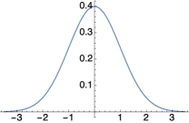
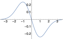
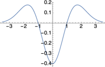
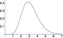
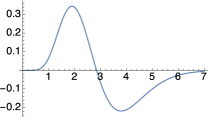
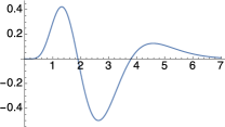
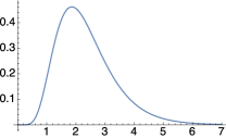
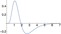
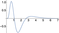
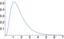
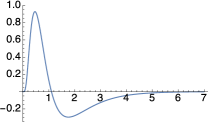
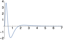
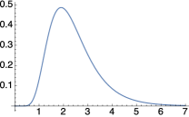
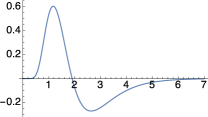
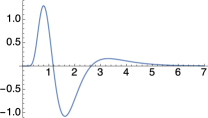
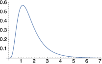
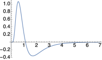
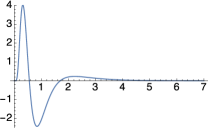
For processing temporal signals at multiple temporal scales, different types of temporal scale-space concepts have been developed in the computer vision literature (see Figure 1):
For off-line processing of pre-recorded signals, a non-causal Gaussian temporal scale-space concept may in many situations be sufficient. A Gaussian temporal scale-space concept is constructed over the 1-D temporal domain in a similar manner as a Gaussian spatial scale-space concept is constructed over a D-dimensional spatial domain (Iijima Iij62 ; Witkin Wit83 ; Koenderink Koe84-BC ; Koenderink and van Doorn KoeDoo92-PAMI ; Lindeberg Lin93-Dis ; Lin94-SI ; Lin10-JMIV ; Florack Flo97-book ; ter Haar Romeny Haa04-book ), with or without the difference that a model for temporal delays may or may not be additionally included (Lindeberg Lin10-JMIV ).
When processing temporal signals in real time, or when modelling sensory processes in biological perception computationally, it is on the other hand necessary to base the temporal analysis on time-causal operations.
The first time-causal temporal scale-space concept was developed by Koenderink Koe88-BC , who proposed to apply Gaussian smoothing on a logarithmically transformed time axis with the present moment mapped to the unreachable infinity. This temporal scale-space concept does, however, not have any known time-recursive formulation. Formally, it requires an infinite memory of the past and has therefore not been extensively applied in computational applications.
Lindeberg Lin90-PAMI ; Lin15-SSVM ; Lin16-JMIV and Lindeberg and Fagerström LF96-ECCV proposed a time-causal temporal scale-space concept based on truncated exponential kernels or equivalently first-order integrators coupled in cascade, based on theoretical results by Schoenberg Sch50 (see also Schoenberg Sch88-book and Karlin Kar68 ) implying that such kernels are the only variation-diminishing kernels over a 1-D temporal domain that guarantee non-creation of new local extrema or equivalently zero-crossings with increasing temporal scale. This temporal scale-space concept is additionally time-recursive and can be implemented in terms of computationally highly efficient first-order integrators or recursive filters over time. This theory has been recently extended into a scale-invariant time-causal limit kernel (Lindeberg Lin16-JMIV ), which allows for scale invariance over the temporal scaling transformations that correspond to exact mappings between the temporal scale levels in the temporal scale-space representation based on a discrete set of logarithmically distributed temporal scale levels.
Based on semi-groups that guarantee either self-similarity over temporal scales or non-enhancement of local extrema with increasing temporal scales, Fagerström Fag05-IJCV and Lindeberg Lin10-JMIV have derived time-causal semi-groups that allow for a continuous temporal scale parameter and studied theoretical properties of these kernels.
Concerning temporal processing over discrete time, Fleet and Langley FleLan95-PAMI performed temporal filtering for optic flow computations based on recursive filters over time. Lindeberg Lin90-PAMI ; Lin15-SSVM ; Lin16-JMIV and Lindeberg and Fagerström LF96-ECCV showed that first-order recursive filters coupled in cascade constitutes a natural time-causal scale-space concept over discrete time, based on the requirement that the temporal filtering over a 1-D temporal signal must not increase the number of local extrema or equivalently the number of zero-crossings in the signal. In the specific case when all the time constants in this model are equal and tend to zero while simultaneously increasing the number of temporal smoothing steps in such a way that the composed temporal variance is held constant, these kernels can be shown to approach the temporal Poisson kernel LF96-ECCV . If on the other hand the time constants of the first-order integrators are chosen so that the temporal scale levels become logarithmically distributed, these temporal smoothing kernels approach a discrete approximation of the time-causal limit kernel Lin16-JMIV .
Applications of using these linear temporal scale-space concepts for modelling the temporal smoothing step in visual and auditory receptive fields have been presented by Lindeberg Lin97-ICSSTCV ; CVAP257 ; Lin10-JMIV ; Lin13-BICY ; Lin13-PONE ; Lin15-SSVM ; Lin16-JMIV , ter Haar Romeny et al. RomFloNie01-SCSP , Lindeberg and Friberg LinFri15-PONE ; LinFri15-SSVM and Mahmoudi Mah16-JMIV . Non-linear spatio-temporal scale-space concepts have been proposed by Guichard Gui98-TIP . Applications of the non-causal Gaussian temporal scale-space concept for computing spatio-temporal features have been presented by Laptev and Lindeberg LapLin03-ICCV ; LapLin04-ECCVWS ; LapCapSchLin07-CVIU , Kläser et al. KlaMarSch08-BMVC , Willems et al. WilTuyGoo08-ECCV , Wang et al. WanUllKlaLapSch09-BMVC , Shao and Mattivi ShaMatt10-CIVR and others, see specifically Poppe Pop09-IVC for a survey of early approaches to vision-based human human action recognition, Jhuang et al. JhuSerWolPog07-ICCV and Niebles et al. NieWanFei08-IJCV for conceptually related non-causal Gabor approaches, Adelson and Bergen AdeBer85-JOSA and Derpanis and Wildes DerWil12-PAMI for closely related spatio-temporal orientation models and Han et al. HanXuZhu15-JMIV for a related mid-level temporal representation termed the video primal sketch.
Applications of the temporal scale-space model based on truncated exponential kernels with equal time constants coupled in cascade and corresponding to Laguerre functions (Laguerre polynomials multiplied by a truncated exponential kernel) for computing spatio-temporal features have presented by Rivero-Moreno and Bres RivBre04-ImAnalRec , Shabani et al. ShaClaZel12-BMVC and Berg et al. BerReyRid14-SensMEMSElOptSyst as well as for handling time scales in video surveillance (Jacob and Pless JacPle08-CircSystVidTech ), for performing edge preserving smoothing in video streams (Paris Par08-ECCV ) and is closely related to Tikhonov regularization as used for image restoration by e.g. Surya et al. SurVorPelJosSeePal15-JMIV . A general framework for performing spatio-temporal feature detection based on the temporal scale-space model based on truncated exponential kernels coupled in cascade with specifically the both theoretical and practical advantages of using logarithmic distribution of the intermediated temporal scale levels in terms of temporal scale invariance and better temporal dynamics (shorter temporal delays) has been presented in Lindeberg Lin16-JMIV .
2.2 Relative advantages of different temporal scale spaces
When developing a temporal scale selection mechanism over a time-causal temporal domain, a first problem concerns what time-causal scale-space concept to base the multi-scale temporal analysis upon. The above reviewed temporal scale-space concepts have different relative advantages from a theoretical and computational viewpoint. In this section, we will perform an in-depth examination of the different temporal scale-space concepts that have been developed in the literature, which will lead us to a class of time-causal scale-space concepts that we argue is particularly suitable with respect to the set of desirable properties we aim at.
The non-causal Gaussian temporal scale space is in many cases the conceptually easiest temporal scale-space concept to handle and to study analytically (Lindeberg Lin10-JMIV ). The corresponding temporal kernels are scale invariant, have compact closed-form expressions over both the temporal and frequency domains and obey a semi-group property over temporal scales. When applied to pre-recorded signals, temporal delays can if desirable be disregarded, which eliminates any need for temporal delay compensation. This scale-space concept is, however, not time-causal and not time-recursive, which implies fundamental limitations with regard to real-time applications and realistic modelling of biological perception.
Koenderink’s scale-time kernels Koe88-BC are truly time-causal, allow for a continuous temporal scale parameter, have good temporal dynamics and have a compact explicit expression over the temporal domain. These kernels are, however, not time-recursive, which implies that they in principle require an infinite memory of the past (or at least extended temporal buffers corresponding to the temporal extent to which the infinite support temporal kernels are truncated at the tail). Thereby, the application of Koenderink’s scale-time model to video analysis implies that substantial temporal buffers are needed when implementing this non-recursive temporal scale-space in practice. Similar problems with substantial need for extended temporal buffers arise when applying the non-causal Gaussian temporal scale-space concept to offline analysis of extended video sequences. The algebraic expressions for the temporal kernels in the scale-time model are furthermore not always straightforward to handle and there is no known simple expression for the Fourier transform of these kernels or no known simple explicit cascade smoothing property over temporal scales with respect to the regular (untransformed) temporal domain. Thereby, certain algebraic calculations with the scale-time kernels may become quite complicated.
The temporal scale-space kernels obtained by coupling truncated exponential kernels or equivalently first-order integrators in cascade are both truly time-causal and truly time-recursive (Lindeberg Lin90-PAMI ; Lin15-SSVM ; Lin16-JMIV ; Lindeberg and Fagerström LF96-ECCV ). The temporal scale levels are on the other hand required to be discrete. If the goal is to construct a real-time signal processing system that analyses continuous streams of signal data in real time, one can however argue that a restriction of the theory to a discrete set of temporal scale levels is less of a contraint, since the signal processing system anyway has to be based on a finite amount of sensors and hardware/wetware for sampling and processing the continuous stream of signal data.
In the special case when all the time constants are equal, the corresponding temporal kernels in the temporal scale-space model based on truncated exponential kernels coupled in cascade have compact explicit expressions that are easy to handle both in the temporal domain and in the frequency domain, which simplifies theoretical analysis. These kernels obey a semi-group property over temporal scales, but are not scale invariant and lead to slower temporal dynamics when a larger number of primitive temporal filters are coupled in cascade (Lindeberg Lin15-SSVM ; Lin16-JMIV ).
In the special case when the temporal scale levels in this scale-space model are logarithmically distributed, these kernels have a manageable explicit expression over the Fourier domain that enables some closed-form theoretical calculations. Deriving an explicit expression over the temporal domain is, however, harder, since the explicit expression then corresponds to a linear combination of truncated exponential filters for all the time constants, with the coefficients determined from a partial fraction expansion of the Fourier transform, which may lead to rather complex closed-form expressions. Thereby certain analytical calculations may become harder to handle. As shown in Lin16-JMIV and Appendix C, some such calculations can on the other hand be well approximated via a scale-time approximation of the time-causal temporal scale-space kernels. When using a logarithmic distribution of the temporal scales, the composed temporal kernels do however have very good temporal dynamics and much better temporal dynamics compared to corresponding kernels obtained by using truncated exponential kernels with equal time constants coupled in cascade. Moreover, these kernels lead to a computationally very efficient numerical implementation. Specifically, these kernels allow for the formulation of a time-causal limit kernel that obeys scale invariance under temporal scaling transformations, which cannot be achieved if using a uniform distribution of the temporal scale levels (Lindeberg Lin15-SSVM ; Lin16-JMIV ).
The temporal scale-space representations obtained from the self-similar time-causal semi-groups have a continuous scale parameter and obey temporal scale invariance (Fagerström Fag05-IJCV ; Lindeberg Lin10-JMIV ). These kernels do, however, have less desirable temporal dynamics (see Appendix A for a general theoretical argument about undesirable consequences of imposing a temporal semi-group property on temporal kernels with temporal delays) and/or lead to pseudodifferential equations that are harder to handle both theoretically and in terms of computational implementation. For these reasons, we shall not consider those time-causal semi-groups further in this treatment.
2.3 Previous work on methods for scale selection
A general framework for performing scale selection for local differential operations was proposed in Lindeberg Lin93-SCIA ; Lin93-Dis based on the detection of local extrema over scale of scale-normalized derivative expressions and then refined in Lindeberg Lin97-IJCV ; Lin98-IJCV — see Lindeberg Lin99-CVHB ; Lin14-EncCompVis for tutorial overviews.
This scale selection approach has been applied to a large number of feature detection tasks over spatial image domains including detection of scale-invariant interest points (Lindeberg Lin97-IJCV ; Lin12-JMIV , Mikolajczyk and Schmid MikSch04-IJCV ; Tuytelaars and Mikolajczyk TuyMik08-Book ), performing feature tracking (Bretzner and Lindeberg BL97-CVIU ), computing shape from texture and disparity gradients (Lindeberg and Gårding LG93-ICCV ; Gårding and Lindeberg GL94-IJCV ), detecting 2-D and 3-D ridges (Lindeberg Lin98-IJCV ; Sato et al. SatNakShiAtsYouKolGerKik98-MIA ; Frangi et al. FraNieHooWalVie00-MED ; Krissian et al. KriMalAyaValTro00-CVIU ), computing receptive field responses for object recognition (Chomat et al. ChoVerHalCro00-ECCV ; Hall et al. HalVerCro00-ECCV ), performing hand tracking and hand gesture recognition (Bretzner et al. BreLapLin02-FG ) and computing time-to-collision (Negre et al. NegBraCroLau08-ExpRob ).
Specifically, very successful applications have been achieved in the area of image-based matching and recognition (Lowe Low04-IJCV ; Bay et al. BayEssTuyGoo08-CVIU ; Lindeberg Lin12-Scholarpedia ; Lin15-JMIV ). The combination of local scale selection from local extrema of scale-normalized derivatives over scales (Lindeberg Lin93-Dis ; Lin97-IJCV ) with affine shape adaptation (Lindeberg and Garding LG96-IVC ) has made it possible to perform multi-view image matching over large variations in viewing distances and viewing directions (Mikolajczyk and Schmid MikSch04-IJCV ; Tuytelaars and van Gool TuyGoo04-IJCV ; Lazebnik et al. LazSchPon05-PAMI ; Mikolajczyk et al. MikTuySchZisMatSchKadGoo05-IJCV ; Rothganger et al. RotLazSchPon06-IJCV ). The combination of interest point detection from scale-space extrema of scale-normalized differential invariants (Lindeberg Lin93-Dis ; Lin97-IJCV ) with local image descriptors (Lowe Low04-IJCV ; Bay et al. BayEssTuyGoo08-CVIU ) has made it possible to design robust methods for performing object recognition of natural objects in natural environments with numerous applications to object recognition (Lowe Low04-IJCV ; Bay et al. BayEssTuyGoo08-CVIU ), object category classification (Bosch et al. BosZisMun07-ICCV ; Mutch and Lowe MutLow08-IJCV ), multi-view geometry (Hartley and Zisserman HarZis04-Book ), panorama stitching (Brown and Lowe BroLow07-IJCV ), automated construction of 3-D object and scene models from visual input (Brown and Lowe BroLow05-3DIM ; Agarwal et al. AgaSnaSimSeiSze09-ICCV ), synthesis of novel views from previous views of the same object (Liu LiuYueTor11-PAMI ), visual search in image databases (Lew et al. LewSebDjeJai06-ACM-Multi ; Datta et al. DatJosLiWan08-CompSurv ), human computer interaction based on visual input (Porta Por02-HumCompStud ; Jaimes and Sebe JaiSeb07-CVIU ), biometrics (Bicego et al. BicLagGroTis06-CVPRW ; Li Li09-EncBiometr ) and robotics (Se et al. SeLowLit05-TROB ; Siciliano and Khatib SicKha08-HandBookRob ).
Alternative approaches for performing scale selection over spatial image domains have also been proposed in terms of (i) detecting peaks of weighted entropy measures (Kadir and Brady KadBra01-IJCV ) or Lyaponov functionals (Sporring et al. SpoCoilTra00-ICIP ) over scales, (ii) minimising normalized error measures over scale (Lindeberg Lin97-IVC ), (iii) determining minimum reliable scales for edge detection based on a noise suppression model (Elder and Zucker EldZuc98-PAMI ), (iv) determining at what scale levels to stop in non-linear diffusion-based image restoration methods based on similarity measurements relative to the original image data (Mrázek and Navara MraNav03-IJCV ), (v) by comparing reliability measures from statistical classifiers for texture analysis at multiple scales (Kang et al. KanMorNag05-ScSp ), (vi) by computing image segmentations from the scales at which a supervised classifier delivers class labels with the highest reliability measure (Loog et al. LooLiTax09-LNCS ; Li et al. LiTaxLoo11-ScSp ), (vii) selecting scales for edge detection by estimating the saliency of elongated edge segments (Liu et al. LiuWanYaoZha12-CVPR ) or (viii) considering subspaces generated by local image descriptors computed over multiple scales (Hassner et al. HasMayZel12-CVPR ).
More generally, spatial scale selection can be seen as a specific instance of computing invariant receptive field responses under natural image transformations, to (i) handle objects in the world of different physical size and to account for scaling transformations caused by the perspective mapping, and with extensions to (ii) affine image deformations to account for variations in the viewing direction and (iii) Galilean transformations to account for relative motions between objects in the world and the observer as well as to (iv) illumination variations (Lindeberg Lin13-PONE ).
Early theoretical work on temporal scale selection in a time-causal scale space was presented in Lindeberg Lin97-AFPAC with primary focus on the temporal Poisson scale-space, which possesses a temporal semi-group structure over a discrete time-causal temporal domain while leading to long temporal delays (see Appendix A for a general theoretical argument). Temporal scale selection in non-causal Gaussian spatio-temporal scale space has been used by Laptev and Lindeberg LapLin03-ICCV and Willems et al. WilTuyGoo08-ECCV for computing spatio-temporal interest points, however, with certain theoretical limitations that are explained in a companion paper Lin16-spattempscsel .111The spatio-temporal scale selection method in (Laptev and Lindeberg LapLin03-ICCV ) is based on a spatio-temporal Laplacian operator that is not scale covariant under independent relative scaling transformations of the spatial vs. the temporal domains Lin16-spattempscsel , which implies that the spatial and temporal scale estimate will not be robust under independent variabilities of the spatial and temporal scales in video data. The spatio-temporal scale selection method applied to the determinant of the spatio-temporal Hessian in (Willems et al. WilTuyGoo08-ECCV ) does not make use of the full flexibility of the notion of -normalized derivative operators Lin16-spattempscsel and has not previously been developed over a time-causal spatio-temporal domain. The purpose of this article is to present a much further developed and more general theory for temporal scale selection in time-causal scale spaces over continuous temporal domains and to analyse the theoretical scale selection properties for different types of model signals.
3 Scale selection properties for the non-causal Gaussian temporal scale space concept
In this section, we will present an overview of theoretical properties that will hold if the Gaussian temporal scale-space concept is applied to a non-causal temporal domain, if additionally the scale selection mechanism that has been developed for a non-causal spatial domain is directly transferred to a non-causal temporal domain. The set of temporal scale-space properties that we will arrive at will then be used as a theoretical base-line for developing temporal scale-space properties over a time-causal temporal domain.
3.1 Non-causal Gaussian temporal scale-space
Over a one-dimensional temporal domain, axiomatic derivations of a temporal scale-space representation based on the assumptions of (i) linearity, (ii) temporal shift invariance, (iii) semi-group property over temporal scale, (iv) sufficient regularity properties over time and temporal scale and (v) non-enhancement of local extrema imply that the temporal scale-space representation
| (1) |
should be generated by convolution with possibly time-delayed temporal kernels of the form (Lindeberg Lin10-JMIV )
| (2) |
where is a temporal scale parameter corresponding to the variance of the Gaussian kernel and is a temporal delay. Differentiating the kernel with respect to time gives
| (3) | ||||
| (4) | ||||
see the top row in Figure 1 for graphs. When analyzing pre-recorded temporal signals, it can be preferable to set the temporal delay to zero, leading to temporal scale-space kernels having a similar form as spatial Gaussian kernels:
| (5) |
3.2 Temporal scale selection from scale-normalized derivatives
As a conceptual background to the treatments that we shall later develop regarding temporal scale selection in time-causal temporal scale spaces, we will in this section describe the theoretical structure that arises by transferring the theory for scale selection in a Gaussian scale space over a spatial domain to the non-causal Gaussian temporal scale space:
Given the temporal scale-space representation of a temporal signal obtained by convolution with the Gaussian kernel according to (1), temporal scale selection can be performed by detecting local extrema over temporal scales of differential expressions expressed in terms of scale-normalized temporal derivatives at any scale according to (Lindeberg Lin97-IJCV ; Lin98-IJCV ; Lin99-CVHB ; Lin14-EncCompVis )
| (6) |
where is the scale-normalized temporal variable, is the order of temporal differentiation and is a free parameter. It can be shown (Lin97-IJCV, , Section 9.1) that this notion of -normalized derivatives corresponds to normalizing the th order Gaussian derivatives over a one-dimensional domain to constant -norms over scale
| (7) |
with
| (8) |
where the perfectly scale invariant case corresponds to -normalization for all orders of temporal differentiation.
Temporal scale invariance.
A general and very useful scale invariant property that results from this construction of the notion of scale-normalized temporal derivatives can be stated as follows: Consider two signals and that are related by a temporal scaling transformation
| (9) |
and assume that there is a local extremum over scales at in a differential expression defined as a homogeneous polynomial of Gaussian derivatives computed from the scale-space representation of the original signal . Then, there will be a corresponding local extremum over scales at in the corresponding differential expression computed from the scale-space representation of the rescaled signal (Lin97-IJCV, , Section 4.1).
This scaling result holds for all homogeneous polynomial differential expression and implies that local extrema over scales of -normalized derivatives are preserved under scaling transformations. Specifically, this scale invariant property implies that if a local scale temporal level level in dimension of time is selected to be proportional to the temporal scale estimate such that , then if the temporal signal is transformed by a temporal scale factor , the temporal scale estimate and therefore also the selected temporal scale level will be transformed by a similar temporal factor , implying that the selected temporal scale levels will automatically adapt to variations in the characteristic temporal scale of the signal. Thereby, such local extrema over temporal scale provide a theoretically well-founded way to automatically adapt the scale levels to local scale variations.
Specifically, scale-normalized scale-space derivatives of order at corresponding temporal moments will be related according to
| (10) |
which means that implies perfect scale-invariance in the sense that the -normalized derivatives at corresponding points will be equal. If , the difference in magnitude can on the other hand be easily compensated for using the scale values of the corresponding scale-adaptive image features (see below).
3.3 Temporal peak
For a temporal peak modelled as a Gaussian function with variance
| (11) |
it can be shown that scale selection from local extrema over scale of second-order scale-normalized temporal derivatives
| (12) |
implies that the scale estimate at the position of the peak will be given by (Lindeberg (Lin98-IJCV, , Equation (56)) (Lin12-JMIV, , Equation (212)))
| (13) |
If we require the scale estimate to reflect the temporal duration of the peak such that
| (14) |
then this implies
| (15) |
which in the specific case of corresponds to (Lin98-IJCV, , Section 5.6.1)
| (16) |
and in turn corresponding to -normalization for according to (8).
If we additionally renormalize the original Gaussian peak to having maximum value equal to one
| (17) |
then if using the same value of for computing the magnitude response as for selecting the temporal scale, the maximum magnitude value over scales will be given by
| (18) |
and will not be independent of the temporal scale of the original peak unless . If on the other hand using as motivated by requirements of scale calibration (14) for , the scale dependency will for a Gaussian peak be of the form
| (19) |
To get a scale-invariant magnitude measure for comparing the responses of second-order temporal derivative responses at different temporal scales for the purpose of scale calibration, we should therefore consider a scale-invariant magnitude measure for peak detection of the form
| (20) |
which for a Gaussian temporal peak will assume the value
| (21) |
Specifically, this form of post-normalization corresponds to computing the scale-normalized derivatives for at the selected scale (14) of the temporal peak, which according to (8) corresponds to -normalization of the second-order temporal derivative kernels.
3.4 Temporal onset ramp
If we model a temporal onset ramp with temporal duration as the primitive function of the Gaussian kernel with variance
| (22) |
it can be shown that scale selection from local extrema over scale of first-order scale-normalized temporal derivatives
| (23) |
implies that the scale estimate at the central position will be given by (Lin98-IJCV, , Equation (23))
| (24) |
If we require this scale estimate to reflect the temporal duration of the ramp such that
| (25) |
then this implies
| (26) |
which in the specific case of corresponds to (Lin98-IJCV, , Section 4.5.1)
| (27) |
and in turn corresponding to -normalization for according to (8).
If using the same value of for computing the magnitude response as for selecting the temporal scale, the maximum magnitude value over scales will be given by
| (28) |
which is not independent of the temporal scale of the original onset ramp unless . If using for temporal scale selection, the selected temporal scale according to (24) would, however, become infinite. If on the other hand using as motivated by requirements of scale calibration (25) for , the scale dependency will for a Gaussian onset ramp be of the form
| (29) |
To get a scale-invariant magnitude measure for comparing the responses of first-order temporal derivative responses at different temporal scales, we should therefore consider a scale-invariant magnitude measure for ramp detection of the form
| (30) |
which for a Gaussian onset ramp will assume the value
| (31) |
Specifically, this form of post-normalization corresponds to computing the scale-normalized derivatives for at the selected scale (25) of the onset ramp and thus also to -normalization of the first-order temporal derivative kernels for .
3.5 Temporal sine wave
For a signal defined as a temporal sine wave
| (32) |
it can be shown that there will be a peak over temporal scales in the magnitude of the th order temporal derivative at temporal scale (Lin97-IJCV, , Section 3)
| (33) |
If we define a temporal scale parameter of dimension according to , then this implies that the scale estimate is proportional to the wavelength of the sine wave according to (Lin97-IJCV, , Equation (9))
| (34) |
and does in this respect reflect a characteristic time constant over which the temporal phenomena occur. Specifically, the maximum magnitude measure over scale (Lin97-IJCV, , Equation (10))
| (35) |
is for independent of the angular frequency of the sine wave and thereby scale invariant.
In the following, we shall investigate how these scale selection properties can be transferred to two types of time-causal temporal scale-space concepts.
4 Scale selection properties for the time-causal temporal scale space concept based on first-order integrators with equal time constants
In this section, we will present a theoretical analysis of the scale selection properties that are obtained in the time-causal scale-space based on truncated exponential kernels coupled in cascade, for the specific case of a uniform distribution of the temporal scale levels in units of the composed variance of the composed temporal scale-space kernels, and corresponding to the time-constants of all the primitive truncated exponential kernels being equal.
We will study three types of idealized model signals for which closed-form theoretical analysis is possible: (i) a temporal peak modelled as a set of truncated exponential kernels with equal time constants coupled in cascade, (ii) a temporal onset ramp modelled as the primitive function of the temporal peak model and (iii) a temporal sine wave. Specifically, we will analyse how the selected scale levels obtained from local extrema of temporal derivatives over scale relate to the temporal duration of a temporal peak or a temporal onset ramp alternatively how the selected scale levels depends on the the wavelength of a sine wave.
We will also study how good approximation the scale-normalized magnitude measure at the maximum over temporal scales is compared to the corresponding fully scale-invariant magnitude measures that are obtained from the non-causal temporal scale concept as listed in Section 3.
4.1 Time-causal scale space based on truncated exponential kernels with equal time constants coupled in cascade
Given the requirements that the temporal smoothing operation in a temporal scale-space representation should obey (i) linearity, (ii) temporal shift invariance, (iii) temporal causality and (iv) guarantee non-creation of new local extrema or equivalently new zero-crossings with increasing temporal scale for any one-dimensional temporal signal, it can be shown (Lindeberg Lin90-PAMI ; Lin15-SSVM ; Lin16-JMIV ; Lindeberg and Fagerström LF96-ECCV ) that the temporal scale-space kernels should be constructed as a cascade of truncated exponential kernels of the form
| (36) |
If we additionally require the time constants of all such primitive kernels that are coupled in cascade to be equal, then this leads to a composed temporal scale-space kernel of the form
| (37) |
corresponding to Laguerre functions (Laguerre polynomials multiplied by a truncated exponential kernel) and also equal to the probability density function of the Gamma distribution having a Laplace transform of the form
| (38) | ||||
Differentiating the temporal scale-space kernel with respect to time gives
| (39) | ||||
| (40) | ||||
see the second row in Figure 1 for graphs. The -norms of these kernels are given by
| (41) | ||||
| (42) | ||||
The temporal scale level at level corresponds to temporal variance and temporal standard deviation .
4.2 Temporal peak
Consider an input signal defined as a time-causal temporal peak corresponding to filtering a delta function with first-order integrators with time constants coupled in cascade:
| (43) |
With regard to the application area of vision, this signal can be seen as an idealized model of an object with temporal duration that first appears and then disappears from the field of view, and modelled on a form to be algebraically compatible with the algebra of the temporal receptive fields. With respect to the application area of hearing, this signal can be seen as an idealized model of a beat sound over some frequency range of the spectrogram, also modelled on a form to be compatible with the algebra of the temporal receptive fields.
| Scale estimate and maximum magnitude from temporal peak (uniform distr) | ||||
|---|---|---|---|---|
| (var, ) | (var, ) | (var, ) | (, ) | |
| 4 | 3.1 | 0.504 | 6.1 | 10.3 |
| 8 | 7.1 | 0.502 | 14.1 | 18.3 |
| 16 | 15.1 | 0.501 | 30.1 | 34.3 |
| 32 | 31.1 | 0.500 | 62.1 | 66.3 |
| 64 | 63.1 | 0.500 | 126.1 | 130.3 |
| Scale estimate and maximum magnitude from temporal ramp (uniform distr) | ||||
|---|---|---|---|---|
| (var, ) | (, ) | (var, ) | (, ) | |
| 4 | 3.2 | 3.6 | 0.282 | 0.254 |
| 8 | 7.2 | 7.7 | 0.282 | 0.272 |
| 16 | 15.2 | 15.8 | 0.282 | 0.277 |
| 32 | 31.2 | 31.8 | 0.282 | 0.279 |
| 64 | 63.2 | 64.0 | 0.282 | 0.281 |
Define the temporal scale-space representation by convolving this signal with the temporal scale-space kernel (43) corresponding to first-order integrators having the same time constants
| (44) | ||||
where we have applied the semi-group property that follows immediately from the corresponding Laplace transforms
| (45) | ||||
By differentiating the temporal scale-space representation (LABEL:eq-temp-scsp-peak-uni-distr) with respect to time we obtain
| (46) | ||||
| (47) | ||||
implying that the maximum point is assumed at
| (48) |
and the inflection points at
| (49) | ||||
| (50) | ||||
This form of the expression for the time of the temporal maximum implies that the temporal delay of the underlying peak and the temporal delay of the temporal scale-space kernel are not fully additive, but instead composed according to
| (51) |
If we define the temporal duration of the peak as the distance between the inflection points, if furthermore follows that this temporal duration is related to the temporal duration of the original peak and the temporal duration of the temporal scale-space kernel according to
| (52) | ||||
Notably these expressions are not scale invariant, but instead strongly dependent on a preferred temporal scale as defined by the time constant of the primitive first-order integrators that define the uniform distribution of the temporal scales.
Scale-normalized temporal derivatives.
When using temporal scale normalization by variance-based normalization, the first- and second-order scale-normalized derivatives are given by
| (53) | ||||
| (54) | ||||
where , and with and according to (46) and (LABEL:eq-temp2der-scsp-peak-uni-distr).
When using temporal scale normalization by -normalization, the first- and second-order scale-normalized derivatives are on the other hand given by (Lindeberg (Lin16-JMIV, , Equation (75)))
| (55) | ||||
| (56) | ||||
with the scale-normalization factors determined such that the -norm of the scale-normalized temporal derivative computation kernel
| (57) |
equals the -norm of some other reference kernel, where we here take the -norm of the corresponding Gaussian derivative kernels (Lindeberg (Lin16-JMIV, , Equation (76)))
| (58) | ||||
for , thus implying
| (59) | ||||
| (60) | ||||
where and denote the -norms (7) of corresponding Gaussian derivative kernels for the value of at which they become constant over scales by -normalization, and the -norms and of the temporal scale-space kernels and for the specific case of are given by (LABEL:eq-L1norm-temp1der-uni-distr) and (LABEL:eq-L1norm-temp2der-uni-distr).
Temporal scale selection.
Let us assume that we want to register that a new object has appeared by a scale-space extremum of the scale-normalized second-order derivative response.
To determine the temporal moment at which the temporal event occurs, we should formally determine the time where , which by our model (54) would correspond to solving a third-order algebraic equation. To simplify the problem, let us instead approximate the temporal position of the peak in the second-order derivative by the temporal position of the peak according to (48) in the signal and study the evolution properties over scale of
| (61) |
In the case of variance-based normalization for a general value of , we have
| (62) | ||||
and in the case of -normalization for
| (63) | ||||
To determine the scale at which the local maximum is assumed, let us temporarily extend this definition to continuous values of and differentiate the corresponding expressions with respect to . Solving the equation
| (64) |
numerically for different values of then gives the dependency on the scale estimate as function of shown in Table 2 for variance-based normalization with either or and -normalization for .
As can be seen from the results in Table 2, when using variance-based scale normalization for , the scale estimate closely follows the scale of the temporal peak and does therefore imply a good approximate transfer of the scale selection property (14) to this temporal scale-space concept. If one would instead use variance-based normalization for or -normalization for , then that would, however, lead to substantial overestimates of the temporal duration of the peak.
Furthermore, if we additionally normalize the input signal to having unit contrast, then the corresponding time-causal correspondence to the post-normalized magnitude measure (20)
| (65) | ||||
is for scale estimates proportional to the temporal duration of the underlying temporal peak very close to constant under variations of the temporal duration of the underlying temporal peak as determined by the parameter , thus implying a good approximate transfer of the scale selection property (21).
4.3 Temporal onset ramp
Consider an input signal defined as a time-causal onset ramp corresponding to the primitive function of first-order integrators with time constants coupled in cascade:
| (66) |
With respect to the application area of vision, this signal can be seen as an idealized model of a new object with temporal diffuseness that appears in the field of view and modelled on a form to be algebraically compatible with the algebra of the temporal receptive fields. With respect to the application area of hearing, this signal can be seen as an idealized model of the onset of a new sound in some frequency band of the spectrogram, also modelled on a form to be compatible with the algebra of the temporal receptive fields.
Define the temporal scale-space representation of the signal by convolution with the temporal scale-space kernel (43) corresponding to first-order integrators having the same time constants
| (67) | ||||
Then, the first-order temporal derivative is given by
| (68) | ||||
which assumes its temporal maximum at .
Temporal scale selection.
Let us assume that we are going to detect a new appearing object from a local maximum in the first-order derivative over both time and temporal scales. When using variance-based normalization for a general value of , the scale-normalized response at the temporal maximum in the first-order derivative is given by
| (69) | ||||
When using -normalization for a general value of , the corresponding scale-normalized response is
| (70) | ||||
where the -norm of the first-order scale-space derivative kernel can be expressed in terms of exponential functions, the Gamma function and hypergeometric functions, but is too complex to be written out here. Extending the definition of these expressions to continuous values of and solving the equation
| (71) |
numerically for different values of then gives the dependency on the scale estimate as function of shown in Table 2 for variance-based normalization with or -normalization for .
As can be seen from the numerical results, for both variance-based normalization and -normalization with corresponding values of and , the numerical scale estimates in terms of closely follow the diffuseness scale of the temporal ramp as parameterized by . Thus, for both of these scale normalization models, the numerical results indicate an approximate transfer of the scale selection property (14) to this temporal scale-space model. Additionally, the maximum magnitude values according to (LABEL:eq-Ltnorm-timecausal-ramp) can according to Stirling’s formula be approximated by
| (72) | ||||
and are very stable under variations of the diffuseness scale of the ramp, and thus implying a good transfer of the scale selection property (31) to this temporal scale-space concept.
| scale estimate | max magnitude |
 |
 |
| scale estimate | max magnitude |
 |
 |
4.4 Temporal sine wave
Consider a signal defined as a sine wave
| (73) |
This signal can be seen as a simplified model of a dense temporal texture with characteristic scale defined as the wavelength of the signal. In the application area of vision, this can be seen as an idealized model of watching some oscillating visual phenomena or watching a dense texture that moves relative the gaze direction. In the area of hearing, this could be seen as an idealized model of temporally varying frequencies around some fixed frequency in the spectrogram corresponding to vibrato.
Define the temporal scale-space representation of the signal by convolution with the temporal scale-space kernel (43) corresponding to first-order integrators with equal time constants coupled in cascade
| (74) | ||||
where and denote the magnitude and the argument of the Fourier transform of the temporal scale-space kernel according to
| (75) | ||||
| (76) | ||||
| (77) | ||||
By differentiating (74) with respect to time , it follows that the magnitude of the th order temporal derivative is given by
| (78) |
Temporal scale selection.
Using variance-based temporal scale normalization, the magnitude of the corresponding scale-normalized temporal derivative is given by
| (79) |
Extending this expression to continuous values of and differentiating with respect to implies that the maximum over scale is assumed at scale
| (80) |
with the following series expansion for small values of corresponding to temporal structures of longer temporal duration
| (81) |
Expressing the corresponding scale estimate in terms of dimension length and parameterized in terms of the wavelength of the sine wave
| (82) | ||||
we can see that the dominant term is proportional to the temporal duration of the underlying structures in the signal and in agreement with the corresponding scale selection property (34) of the scale-invariant non-causal Gaussian temporal scale space concept, whereas the overall expression is not scale invariant.
If the wavelength is much longer than the time constant of the primitive first-order integrators, then the scale selection properties in this temporal scale-space model will constitute a better approximation of the corresponding scale selection properties in the scale-invariant non-causal Gaussian temporal scale-space model.
The maximum value over scale is
| (83) |
with the following series expansion for large and :
| (84) |
Again we can note that the first term agrees with the corresponding scale selection property (35) for the scale-invariant non-causal Gaussian temporal scale space, whereas the higher order terms are not scale invariant.
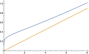
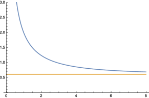
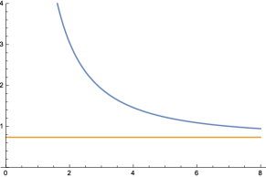
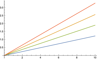
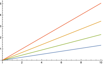
Figure 2 shows graphs of the scale estimate according to (4.4) for and and the maximum response over scale for and as function of the wavelength of the sine wave (marked in blue). For comparison, we also show the corresponding scale estimates (34) and magnitude values (35) that would be obtained using temporal scale selection in the scale-invariant non-causal Gaussian temporal scale space (marked in brown).
As can be seen from the graphs, both the temporal scale estimate and the maximum magnitude obtained from a set of first order integrators with equal time constants coupled in cascade approach the corresponding results obtained from the non-causal Gaussian scale space for larger values of in relation to the time constant of the first-order integrators. The scale estimate obtained from a set of first-order integrators with equal time constants is, however, for lower values of generally significantly higher than the scale estimates obtained from a non-causal Gaussian temporal scale space. The scale-normalized magnitude values, which should be constant over scale for a scale-invariant temporal scale space when according to the scale selection property (35), are for lower values of much higher than the scale-invariant limit value when performing scale selection in the temporal scale-space concept obtained by coupling a set of first-order integrators with equal time constants in cascade. The scale selection properties (34) and (35) are consequently not transferred to this temporal scale-space concept for the sine wave model, which demonstrates the need for using a scale-invariant temporal scale-space concept when formulating mechanisms for temporal scale selection. The scale selection properties of such a scale-invariant time-causal temporal concepts will be analysed in Section 5, and showing that it is possible to obtain temporal scale estimates for a dense sine wave that are truly proportional to the wavelength of the signal, i.e., a characteristic estimate of the temporal duration of the temporal structures in the signal.
Concerning this theoretical analysis, it should be noted that we have here for the expressions (4.4), (83) and (84) disregarded the rounding of the continuous value in (81) to the nearest integer upwards or downwards where it assumes its maximum value over temporal scales. Thereby, the graphs in Figure 2 may appear somewhat different if such quantization effects because of discrete temporal scale levels are also included. The lack of true temporal scale invariance will, however, still prevail.
Concerning the motivation to the theoretical analysis in this section, while the purpose of this analysis has been to investigate how the temporal scale estimates depend on the frequency or the wavelength of the signal, it should be emphasized that the primary purpose has not been to develop a method for only estimating the frequency or the wavelength of a sine wave. Instead, the primary purpose has been to carry out a closed-form theoretical analysis of the properties of temporal scale selection when applied to a model signal for which such closed-form theoretical analysis can be carried out. Compared to using e.g. a Fourier transform for estimating the local frequency content in a signal, it should be noted that the computation of a Fourier transform requires a complementary parameter — a window scale over which the Fourier transform is to be computed. The frequency estimate will then be an average of the frequency content over the entire interval as defined by the window scale parameter. Using the the proposed temporal scale selection methodology it is on the other hand possible to estimate the temporal scale without using any complementary window scale parameter. Additionally, the temporal scale estimate will be instantaneous and not an average over multiple cycles of e.g. a periodic signal, see also the later experimental results that will be presented in Section 7 in particular Figure 8.
5 Scale selection properties for the time-causal temporal scale space concept based on the scale-invariant time-causal limit kernel
In this section, we will analyse the scale selection properties for the time-causal scale-space concept based on convolution with the scale-invariant time-causal limit kernel.
The analysis starts with a detailed study of a sine wave, for which closed-form theoretical analysis is possible and showing that the selected temporal scale level measured in units of dimension time according to will be proportional to the wavelength of the signal, in accordance with true scale invariance. We also show that despite the discrete nature of the temporal scale levels in this temporal scale-space concept, local extrema over scale will nevertheless be preserved under scaling transformations of the form , with denoting the distribution parameter of the time-causal limit kernel.
Then, we present a general result about temporal scale invariance that holds for temporal derivatives of any order and for any input signal, showing that under a temporal scaling transformation of the form , local extrema over scales are preserved under such temporal scaling transformations with the temporal scale estimates transforming according to . We also show that if the scale normalization power corresponding to , the scale-normalized magnitude responses will be preserved in accordance with true temporal scale invariance.
5.1 Time-causal temporal scale space based on the scale-invariant time-causal limit kernel
Given the temporal scale-space model based on truncated exponential kernels (36) coupled in cascade
| (85) |
having a composed Fourier transform of the form
| (86) | ||||
and as arises from the assumptions of (i) linearity, (ii) temporal shift invariance, (iii) temporal causality and (iv) non-creation of new local extrema or equivalently zero-crossings with increasing scale, it is more natural to distribute the temporal scale levels logarithmically over temporal scales
| (87) |
so that the distribution in terms of effective temporal scale (Lindeberg Lin92-PAMI ) becomes uniform. This implies that time constants of the individual first-order integrators should for some be given by (Lindeberg Lin15-SSVM ; Lin16-JMIV )
| (88) | ||||
| (89) | ||||
Specifically, if one lets the number of temporal scale levels tend to infinity with the density of temporal scale levels becoming infinitely dense towards , it can be shown that this leads to a scale-invariant time-causal limit kernel having a Fourier transform of the form (Lindeberg (Lin16-JMIV, , Section 5))
| (90) | ||||
| , | , |
 |
 |
| , | , |
 |
 |
| , | , |
 |
 |
| , | , |
 |
 |
| for | for |
|---|---|
 |
 |
5.2 Temporal sine wave
Consider an input signal defined as a sine wave
| (91) |
and taken as an idealized model of a oscillating signal with temporal structures having characteristic temporal duration .
For the time-causal temporal scale-space defined by convolution with the time-causal semi-group , the temporal scale-space representation is given by
| (92) |
where the magnitude and the argument of the Fourier transform of the time-causal limit kernel are given by
| (93) | ||||
| (94) | ||||
Thus, the magnitude on the th order temporal derivative is given by
| (95) |
and for the th order scale-normalized derivate based on variance-based scale normalization the amplitude as function of scale is
| (96) | ||||
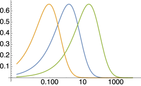
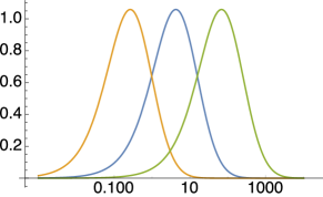
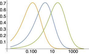
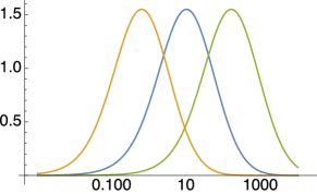
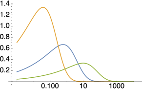
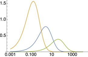
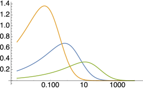
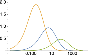
Figure 4 shows graphs of the variation of this entity as function of temporal scale for different angular frequencies , orders of temporal differentiation and the distribution parameter . As can be seen from the graphs, the maxima over scales are assumed at coarser scales with increasing wavelength of the sine wave. The maxima over temporal scale are also assumed at coarser scales for second-order derivatives than for first-order derivatives.
Specifically, when the magnitude values at the local extrema over scale are constant over scale, which implies a transfer of the scale selection property (10) to this temporal scale-space model. Notably, this situation is in clear contrast to the situation for the temporal scale-space generated by first-order integrators with equal time constants coupled in cascade. In Figure 2 it was shown that because of the lack of true temporal scale invariance of that temoral scale-space concept, the maximum magnitude values are not constant over scales for as they should be according to the scale-invariant scale selection property (10).
When choosing lower values of as motivated from the determination of the parameter for scale selection in a Gaussian scale space to make the scale estimate reflect the width of a Gaussian peak for second-order derivatives or reflect the width of a diffuse ramp for first-order derivatives, which leads to for first-order derivatives (27) and for second-order derivatives (16), the local extrema over scale are moved to finer scales (see Figure 4). Then, however, the maximum magnitude values are no longer the same for sine waves of different frequencies, implying that a complementary magnitude normalization step is necessary (see Section 5.3 for additional details).
Local extrema over temporal scale.
Taking the logarithm of the expression (LABEL:eq-magn-sc-norm-ders-sine-wave-limit-kern) gives
| (97) |
If we treat as a continuous variable and differentiate with respect to we obtain
| (98) |
Figure 5 show graphs of how the scale estimate obtained by setting the derivative with respect to temporal scale to zero increases linearly with the wavelength of the signal, with different slopes of the linear curve depending on the order of temporal differentiation and the value of the scale normalization parameter . This overall linear scaling behaviour can directly be proved by rewriting the expression in (98) into
| (99) |
Since this expression is a direct function of the dimensionless entity , it follows that the temporal scale estimates will be of the form
| (100) |
for some function , and thus obeying temporal scale invariance in the sense that the scale estimate in dimension length is proportional to the wavelength of the signal
| (101) |
Notice how this situation is in contrast to the results of scale selection in the temporal scale-space concept obtained by coupling first-order integrators with equal time constants in cascade, where the scale estimate for a sine wave is not directly proportional to the wavelength of the temporal signal, but also affected by a wavelength dependent temporal scale bias (see Equation (4.4) and Figure 2 in Section 4.4).
| Scale estimates for | ||
|---|---|---|
| 1.20 | 2.06 | |
| 0.77 | 1.61 | |
| Scale estimates for | ||
|---|---|---|
| 1.43 | 3.17 | |
| 0.83 | 2.17 | |
| Ratios for | ||
|---|---|---|
| 1.20 | 1.46 | |
| 1.09 | 1.32 | |
| Ratios for | ||
|---|---|---|
| 1.43 | 2.24 | |
| 1.18 | 1.77 | |
Table 4 shows numerical values of the differences between the results for different orders of differentiation and different values of . These numerical entities become particularly illuminating by forming the ratio as shown in Table 4. For a non-causal Gaussian scale space, this ratio should be equal to one for all combinations of and (see Equation (33)). For this non-causal temporal scale space, we can, however, note that the deviation from one increases both with larger values of the distribution parameter222The reason why the these ratios depend on the distribution parameter can specifically be explained by observing that the temporal duration of the temporal derivatives of the time-causal limit kernel will depend on the distribution parameter – see Appendix C for a derivation and explicit estimates of the width of the temporal derivatives of the time-causal limit kernel. and with increasing order of temporal differentiation , which both lead to larger degrees of temporal asymmetry due to the non-causal temporal dimension.
In the essential proportionality of the scale estimate to the wavelength of the signal according to (101), the main component of the scale selection property (34) is thereby transferred to this temporal scale-space concept, although the proportionality constant has to be modified depending on the value of the temporal scale distribution parameter , the order of temporal differentiation and the scale normalization parameter .
Preservation of local extrema over temporal scale under temporal scaling transformations.
Let us assume that the continuous magnitude function (97) assumes a maximum over temporal scales for some pair and that the derivative with respect to temporal scale is thereby zero
| (102) |
Let us next assume that we feed in a different sine wave with wavelength for some integer (for the same value of as used in the definition of the time-causal limit kernel) and corresponding to with its matching scale . Then, it holds that
| (103) | ||||
This result implies that the sign of the derivate with respect to temporal scale is preserved between matching angular frequencies and scales and . Specifically, local extrema over temporal scales are preserved under uniform scaling transformations of the temporal domain , implying scale covariance of the temporal scales that are selected from local extrema over scales of scale-normalized temporal derivatives.
Note also that although the analysis in Equation (LABEL:eq-scale-cov-temp-scsel-sine-wave-limit-kern) is performed based on a temporary extension of into a continuous variable, the scale covariance still holds when the continuous function is sampled into a discrete set of temporal scale levels.333A formal proof of the transfer of this preservation property of local extrema over temporal scales from a temporary extension of the temporal scale parameter into a continuous variable back into a restricted discrete set of temporal scale levels can be stated as follows: From Equation (LABEL:eq-scale-cov-temp-scsel-sine-wave-limit-kern) it follows that the continuous temporal scale-space signatures for the two sine waves of wavelengths and will increase and decrease respectively at corresponding matching temporal scale levels and . If we next sample these scale-space signatures at some discrete set of temporal scale levels and , then it follows that the discrete maxima over temporal scales will also be related according to . This preservation property of local extrema does, however, only hold for temporal scaling factors that are integer powers of the distribution parameter , i.e., only . Alternatively, this preservation property can also be derived from the more general scale invariance property under temporal scaling transformations (LABEL:eq-transf-prop-sc-norm-temp-ders-limit-kern) that is stated in next section.
5.3 General scale invariance property under temporal scaling transformations
In Lindeberg (Lin16-JMIV, , Appendix 3) it is shown that for two temporal signals and that are related by a temporal scaling transform for with the corresponding transformation between corresponding temporal scale levels , the scale-normalized temporal derivatives defined by either -normalization or variance-based normalization in the scale-space representation defined by convolution with the time-causal limit kernel are for any temporal input signal related according to
| (104) | ||||
This result specifically implies that the scale-space signatures, which are the graphs that show the variation in the strength of scale-normalized derivatives over scale, will be rescaled copies of each other for signals that are related by a uniform scaling transformation of the temporal domain.
Specifically, local temporal scale estimates and as determined from local extrema over temporal scales in the two temporal domains will be assumed at corresponding temporal scale levels and will thus be transformed in a scale-covariant way for any temporal scaling transformation of the form . In units of the temporal variance, it holds that
| (105) |
and in units of the temporal standard deviation
| (106) |
If corresponding to , the magnitude values at corresponding temporal scale levels will be equal. If corresponding to , the magnitude values will be related according to (LABEL:eq-transf-prop-sc-norm-temp-ders-limit-kern). Thereby, this expression provides a way to normalize maximum strength measures between local extrema over scales assumed at different temporal scales as obtained e.g. in the scale-space signatures shown in Figure 4.
Note that by this construction we have been able to transfer the temporal scale invariance property (9) and (10) that holds for a non-causal Gaussian temporal scale-space concept to also hold for a time-causal temporal scale-space concept, which is a novel type of theoretical construction. This property is, however, restricted to the temporal scale-space concept based on convolution with the time-causal limit kernel and does, for example, not hold for the time-causal temporal scale-space concept based on convolution with a cascade of truncated exponential kernels having equal time constants and corresponding to a uniform distribution of the temporal scale levels in units of the composed temporal variance.
| Temporal peak for | Scale-space signature |
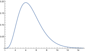 |
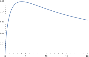 |
| Temporal onset ramp for | Scale-space signature |
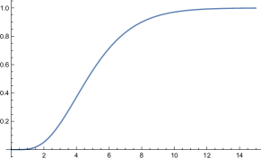 |
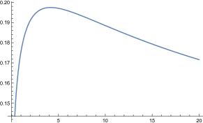 |
| Sine wave for | Scale-space signature |
 |
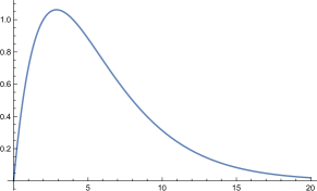 |
| Sine wave for | Scale-space signature |
 |
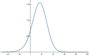 |
6 Influence of discrete temporal scale levels on the theoretical analysis
In the theoretical analysis of scale selection properties of (i) a temporal peak in Section 4.2, (ii) a temporal onset ramp in Section 4.3 and (ii) a temporal sine wave in Section 4.4 and Section 5.2, we did first compute closed-form expressions for how the scale-normalized temporal magnitude measures depend upon the temporal scale levels according to (LABEL:eq-Lttnorm-timecausal-peak), (LABEL:eq-Ltnorm-timecausal-ramp) and (79) for the time-causal scale-space concept based on truncated exponential kernels with equal time constant coupled in cascade or how the scale-normalized magnitude measure depends on the temporal scale level according to (LABEL:eq-magn-sc-norm-ders-sine-wave-limit-kern) for the time-causal temporal scale-space concept based on the scale-invariant limit kernel:
| (107) | ||||
| (108) | ||||
| (109) | ||||
| (110) | ||||
Then, to compute the temporal scale levels at which the scale-normalized derivative responses assumed their maximum values over temporal scales, we temporarily extended these magnitude measures from being defined over discrete integer temporal scale levels to a continuum over , to be able to differentiate the closed-form expressions with respect to the temporal scale level.
A general question that could be raised in this context therefore concerns how good approximation the results from the continuous approximation of local extrema over scales are with respect to a setting where the temporal scale levels are required to be discrete. A common property of the four types of scale-space signatures according to equations (LABEL:eq-M-peak-uni)–(LABEL:eq-M-sine-uni) and shown in Figure 6 is that they are unimodal, i.e., they assume a single maximum over temporal scales and do first increase and then decrease. Thereby, when the continuous variable with its associated maximum over temporal scales obtained from a continuous analysis is in a second stage restricted to be discrete, it follows that the discrete maximum over discrete temporal scales is guaranteed to be assumed at either the nearest lower or the nearest higher integer. Thus, we obtain the discrete temporal scale estimate by rounding the continuous scale estimate to either the nearest lower or the nearest higher integer.
Whether the value should be rounded upwards or downwards depends on how close the continuous estimate is to the nearest downwards vs. upwards integers and on the local degree of asymmetry of the scale-space signature around the maximum over temporal scales.
When implementing and executing a temporal scale selection algorithm in practice, the situation can on the other hand be reverse. Given a set of discrete temporal scale levels, we may detect a local maximum over temporal scales at some discrete temporal scale level . If we would like to use this temporal scale estimate for estimating the temporal duration of the underlying temporal structure that gave rise to the response, e.g. according to the methodology outlined in appendix C, we may on the other hand would like to compute a better continuous estimate of the temporal scale level than as restricted by the discrete temporal scale levels.
A straightforward way of computing a more accurate temporal scale estimate in such a situation is by interpolating a parabola over the measurements over the temporal scale levels in an analogous way as subresolution spatial scale estimates can be obtained over a spatial scale-space representation Lin97-IJCV ; LinBre03-ScSp ; Low04-IJCV . Let denote the scale level and the magnitude measure at the discrete maximum and let and denote the corresponding scale level and magnitude measure at the nearest lower and upper temporal scales, respectively. Assuming the following form of the interpolating function
| (111) |
the interpolation coefficients become
| (112) | ||||
| (113) | ||||
| (114) | ||||
with the corresponding subresolution estimate of the maximum over scales
| (115) |
Note that the correction offset is restricted to the interval implying that the location of the discrete maximum is guaranteed to be on the sampling grid point nearest to the subresolution estimate .
7 Temporal scale selection for 1-D temporal signals
To illustrate the derived scale selection properties, we will in this section show the result of applying temporal scale selection to different types of purely temporal signals.
| Scale-space extrema from the time-causal limit kernel | Scale-space extrema from the non-causal Gaussian kernel |
|---|---|
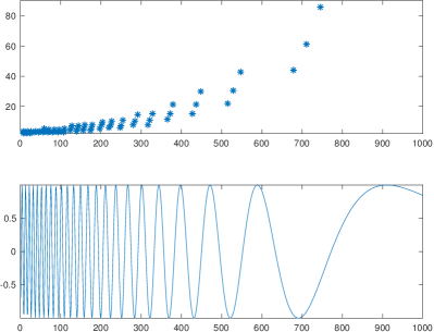 |
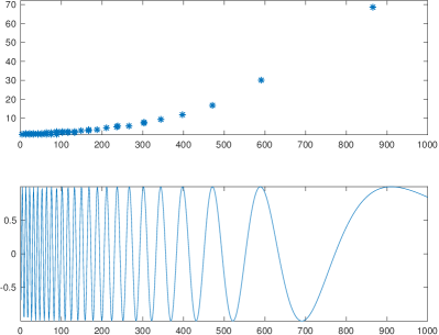 |
| computed with time-causal limit kernel | computed with non-causal Gaussian kernel |
|---|---|
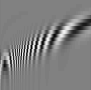 |
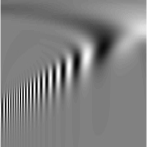 |
The bottom rows in Figure 8 shows a one-dimensional model signal having a temporally varying frequency of the form
| (116) |
defined such that the local wavelength increases with time . Figure 8 shows the temporal scale-space representation of the scale-normalized second-order temporal as function of scale for the maximally scale-invariant choice of corresponding to . Note how structures in the signal of longer temporal duration give rise responses at coarser temporal scales in agreement with the derived theoretical properties of the scale-covariant scale-space concepts over a time-causal vs. a non-causal temporal domain.
In the top rows in Figure 8 we show the results of applying local temporal scale selection by detecting local maxima over both time and scale of the scale-normalized second-order temporal derivative for the scale-calibrated choice of corresponding to . Each detected scale-space extremum has been marked by a star at the point in scale-space at which the local maximum over temporal scale was assumed. Such temporal scale selection has been performed using two types of temporal scale-space concepts: (i) based on the time-causal scale-space representation corresponding to convolution with the scale-invariant limit kernel with distribution parameter approximated by a finite number of the at least slowest primitive smoothing steps at the finest level of scale or (ii) based on the non-causal Gaussian kernel using 5 temporal scale levels per scale octave.
The discrete implementation of the time-causal temporal scale-space representation corresponding to convolution with the scale-invariant limit kernel has been based on recursive filters over time according to the methodology described in Lindeberg (Lin16-JMIV, , section 6.2) whereas the discrete implementation of the non-causal Gaussian temporal scale-space concept has been based on the discrete analogue of the Gaussian kernel described in Lindeberg Lin90-PAMI ; Lin93-JMIV . Discrete implementation of scale-normalized temporal derivatives has in turn been based on discrete -normalization according to the methodology outlined in (Lin16-JMIV, , section 7).
As can be seen from the results in the top rows in Figure 8, the temporal scale estimates increase proportional to the local wavelength according to the derived scale-invariant properties of the temporal scale-space concepts based on convolution with the time-causal limit kernel or the non-causal Gaussian kernel. The scale estimates obtained using the time-causal vs. the non-causal temporal scale space concepts are, however, not equal in units of the standard deviation of the temporal scale-space kernel — see also the theoretical analysis in section 5 with specifically the numerical comparisons in Table 4. Thus, different scale calibration factors are needed to transform the temporal scale estimates in units of the temporal standard deviation to units of the temporal duration of the signal for the time-causal vs. the non-causal Gaussian temporal scale-space concepts — compare with the theoretical analysis in appendix C.
| Post-filtered scale-space extrema from the time-causal limit kernel |
| Delay compensated scale-space extrema from the time-causal limit kernel |
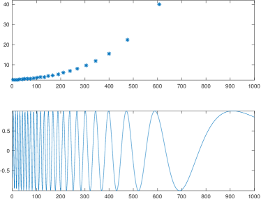 |
| Time-causal peak | Non-causal peak |
 |
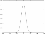 |
| Time-causal scale-space | Non-causal scale-space |
 |
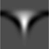 |
| Scale-space extrema from the time-causal limit kernel | Scale-space extrema from the non-causal Gaussian kernel |
|---|---|
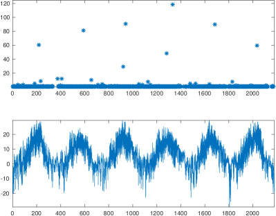 |
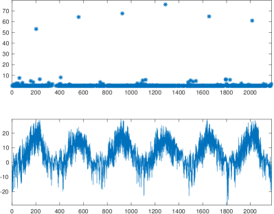 |
| Quasi quadrature computed with time-causal limit kernel | Quasi quadrature computed with non-causal Gaussian kernel |
|---|---|
 |
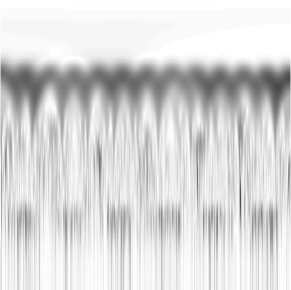 |
Another qualitative difference that can be noted with regard to temporal scale selection in a time-causal temporal scale-space representation vs. a non-causal Gaussian temporal scale-space representation is that any measurement performed in a time-causal temporal scale-space concept is associated with an inherent temporal delay , whereas the temporal delay can be defined to be zero for a non-causal Gaussian temporal scale-space. Thus, the local extrema over scales will be assumed later with increasing temporal scale levels as induced by temporal structures of having longer temporal duration. Varying the parameter in the scale calibration criteria (14) and (25) to values of provides a straightforward way of enforcing responses to be obtained at finer temporal scales and thereby implying shorter temporal delays, at the potential cost of a larger likelihood of false positive responses by not detecting the underlying temporal structures at the same temporal scales as they occur.
Yet another side effect of the longer temporal delays at coarser temporal scales is that multiple local responses over scales may be obtained with respect to the same underlying temporal structure, with first responses obtained at finer temporal scales followed by later responses at coarser temporal scales. Because of the temporal shift caused by different temporal delays between adjacent temporal scale levels, scale-space extrema detection over a local neighbourhood may not detect a single extremum over temporal scales as for the non-causal Gaussian temporal scale-space concept. Therefore, explicit handling of different temporal delays at different temporal scale levels is needed when performing temporal scale selection in a time-causal temporal scale-space representation. The presented theory of temporal scale selection properties is intended to be generally applicable with respect to different such strategies for handling the temporal delays in specific algorithms.
7.1 Post-filtering of responses at adjacent temporal scales
In view of the behaviour of image structures over temporal scales illustrated in Figure 8, one way of suppressing multiple responses to the same underlying structure at different temporal scales is by performing an additional search around each scale-space extremum as follows: If a point at temporal scale level with temporal scale index is a scale-space maximum, perform an additional search at the nearest finer temporal scale level to previous temporal moments as long as the scale-normalized values monotonically increase. When the monotone increase stops and a local temporal maximum has been found, then compare if the temporal maximum value at the nearest finer temporal scale is greater than the temporal maximum value at the current scale. If so, suppress the scale-space maximum at the current scale. In a corresponding manner, perform a search at the next coarser temporal scale to the following temporal moments as long as the scale-normalized values monotonically increase. When the monotone increase stops and a local temporal maximum has been found, then compare if the temporal maximum value at the next coarser temporal scale is greater than the temporal maximum value at the current scale. If so, suppress the scale-space maximum at the current scale. By this type of straightforward scale-space tracking over adjacent temporal scales, a single response will be obtained to the same underlying structure as illustrated in Figure 10. Additionally, a more accurate temporal scale estimate can be computed by performing the parabolic interpolation according to (111) and (115) over the nearest backward and forward temporal maxima at the adjacent finer and coarser temporal scales as opposed to an interpolation over temporal scales at the same temporal moment as at which the temporal scale-space maximum was assumed.
Note that in a real-time situation, the necessary information needed to perform a search to the past can be stored by a process that records the value of temporal maxima at each temporal scale. In a corresponding manner, later deletion or subresolution interpolation of the scale estimate of a scale-space maximum can only be performed when time has passed to the location of the next temporal maximum at the nearest coarser temporal scale. If a preliminary feature response has been obtained at any temporal scale while a potential response at the nearest coarser temporal scale is not available yet because of its longer temporal scale, a real-time system operating over multiple scales should preferably be designed with the ability to correct or adjust preliminary measurements when more information at coarser scales becomes available — see also Figure 11 for an illustration of the underlying temporal dynamics that arises when processing signals at multiple scales using a time-causal temporal scale-space representation.
While these descriptions have been given regarding scale-space maxima and local maxima, the procedure for handling scale-space minima and local minima is analogous with the polarity of the signal reversed.
7.2 Temporal delay compensation
In Figure 10 we have additionally adjusted the temporal location of every temporal scale-space maximum by an estimate of the temporal delay computed from the location of the temporal maximum of the underlying temporal scale-space kernel according to (Lin16-JMIV, , Section 4). Note that although any temporal event detected at a coarser temporal scale will by necessity be associated with non-zero temporal delay, we can nevertheless retrospectively compute a good estimate of when the underlying event occurred that gave rise to the registered feature response.
7.3 Temporal scale selection for a real measurement signal
While a main purpose of this article is to develop a theory of temporal scale selection to be used in conjunction with a spatio-temporal scale-space concept for video analysis or a spectro-temporal scale-space concept for audio analysis, we argue that this theory is applicable to much larger classes of time-dependent measurement signals. For the purpose of isolating the effect to a purely one-dimensional measurement signal, we do in Figure 13 show the result of applying corresponding temporal scale selection to a real measurement signal showing hourly measurements of the temperature at a weather station. Note how the temporal scale selection method based on scale-space extrema is able to extract the coarse scale temperature peaks although the signal contains substantial high-amplitude variations at finer scales.
For the purpose of having the local feature responses being less dependent on the local phase of the signal than for either first- or second-order temporal derivatives or , we do in Figure 13 show the result of computing a quasi quadrature measure
| (117) |
derived in Lin16-spattempscsel to for
| (118) |
constitute an improved version of an earlier proposed quasi quadrature measure in Lindeberg Lin97-AFPAC .
| time-causal | non-causal |
|---|---|
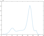 |
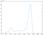 |
| Temporal scale estimates from temporal peaks | |||||
|---|---|---|---|---|---|
| 2 | 2.26 | 2.14 | 2 | 1.58 | 2.16 |
| 4 | 4.11 | 4.05 | 4 | 4.57 | 4.06 |
| 8 | 7.76 | 8.06 | 8 | 8.02 | 7.96 |
| 16 | 15.90 | 16.03 | 16 | 15.60 | 15.86 |
| 32 | 31.97 | 32.06 | 32 | 31.35 | 31.66 |
| 64 | 64.12 | 64.13 | 64 | 63.15 | 63.31 |
| Temporal scale estimates from temporal onset ramps | |||||
|---|---|---|---|---|---|
| 2 | 2.01 | 1.96 | 2 | 2.04 | 1.97 |
| 4 | 3.66 | 3.90 | 4 | 3.68 | 3.98 |
| 8 | 7.71 | 8.02 | 8 | 7.60 | 7.94 |
| 16 | 15.68 | 16.02 | 16 | 15.42 | 15.90 |
| 32 | 32.00 | 32.04 | 32 | 31.48 | 31.77 |
| 64 | 64.08 | 64.08 | 64 | 63.44 | 63.54 |
| Temporal scale estimates from non-causal Gaussian scale space | |||||
|---|---|---|---|---|---|
| temporal peak | temporal onset ramp | ||||
| 2 | 2.95 | 1.92 | 2 | 1.59 | 2.07 |
| 4 | 4.04 | 3.97 | 4 | 3.86 | 4.03 |
| 8 | 8.10 | 7.98 | 8 | 7.92 | 8.02 |
| 16 | 15.89 | 15.99 | 16 | 15.94 | 16.01 |
| 32 | 32.06 | 32.00 | 32 | 31.97 | 32.00 |
| 64 | 64.02 | 64.00 | 64 | 63.97 | 64.00 |
Note how this operator responds to different types of temporal structures at different temporal scales with a particularly strong response due to the temporal variations caused by the daily and annual temperature cycles. This effect becomes more immediately noticeable if we complement the above temporal scale selection method with a complementary assumption about stationarity of the signal and sum up the scale-normalized feature responses of the quasi quadrature measure over time for every temporal scale level. In the graphs shown in Figure 14 we do then obtain two major peaks over temporal scales, with the finer scale peak corresponding to the daily temperature cycle and the coarser scale peak to the annual temperature cycle.
Note that the purpose of this experiment is not primarily to develop an algorithm for detecting periodic variations in a signal but to illustrate that the temporal scale selection mechanism produces intuitively reasonable temporal scale estimates for a real-world 1-D signal with known properties.
7.4 Numerical accuracy of the temporal scale estimates
To investigate how well the temporal scale estimates generated by the resulting temporal scale selection mechanism reflect the temporal scale in the underlying temporal signal, we generated temporal model signals defined as either (i) a temporal peak modelled as time-causal limit kernel with temporal scale and distribution parameter for different values of and and (ii) a temporal onset ramp modelled as the primitive function of the temporal peak model. Then, we detected scale-space extrema of the second-order scale-normalized temporal derivative for peak detection or scale-space extrema of the first-order scale-normalized temporal derivative for onset detection, using the time-causal temporal scale-space concept corresponding to convolution with the time-causal limit kernel for the same value of and resulting in temporal scale estimates .
Table 7 and Table 7 show results from this experiment for the time-causal temporal peak and the temporal onset ramp models, respectively. Note how well the temporal scale estimates derived for truncated exponential kernels with a uniform distribution of the temporal scale levels in section 4.2 and section 4.3 do also generalize to truncated exponential kernels with a logarithmic distribution of the temporal scale levels. Table 7 shows corresponding results for the non-causal Gaussian scale-space concept applied to non-causal temporal peak and temporal onset ramp models, respectively, and again with a very good agreement between the local scale estimates in relation to the inherent temporal scale in the signal.
For this experiment, we can specifically note that variance-based temporal scale normalization does on average lead to slightly more accurate temporal scale estimates compared to discrete -normalization, which can be contrasted to previous results regarding spatial scale selection in hybrid pyramids by Lindeberg and Bretzner LinBre03-ScSp , where -normalization lead to much more accurate scale selection results compared to variance-based normalization.
8 Temporal scale selection in spatio-temporal video data
In this section, we will develop a basic proof of concept of applying the proposed theory and methodology for selecting local temporal scales in video data based on a small set of specific spatio-temporal feature detectors formulated in terms of spatio-temporal differential invariants. A more detailed treatment of this topic with examples for more general families of differential expressions for spatio-temporal scale selection with associated spatio-temporal image models for scale calibration is presented in a companion paper Lin16-spattempscsel .
8.1 Spatio-temporal receptive field model
For applying the proposed framework for temporal scale selection to spatio-temporal video data, we follow the approach with idealized models of spatio-temporal receptive fields of the form
| (119) |
as previously derived, proposed and studied in Lindeberg Lin10-JMIV ; Lin13-BICY ; Lin16-JMIV where
-
•
denotes the image coordinates,
-
•
denotes time,
-
•
denotes the spatial scale,
-
•
denotes the temporal scale,
-
•
denotes a local image velocity,
-
•
denotes a spatial covariance matrix determining the spatial shape of an affine Gaussian kernel ,
-
•
denotes a spatial affine Gaussian kernel that moves with image velocity in space-time and
-
•
is a temporal smoothing kernel over time.
and we specifically here choose as temporal smoothing kernel over time either (i) the time-causal temporal scale-space kernel corresponding to a set of first-order integrators with equal time constants coupled in cascade (37)
| (120) |
with or (ii) the time-causal limit kernel
| (121) |
defined via its Fourier transform of the form (LABEL:eq-FT-comp-kern-log-distr-limit).
For simplicity, we shall in this treatment restrict ourselves to space-time separable receptive fields obtained by setting the image velocity to zero and to receptive fields that are rotationally symmetric over the spatial domain as obtained by setting the spatial covariance matrix to a unit matrix . The resulting spatio-temporal receptive fields that we then obtain correspond to complementing our time-causal temporal scale-space concepts studied in Sections 4–5 with a rotationally symmetric spatial Gaussian scale-space concept over the spatial domain.
Specifically, the natural way of expressing spatio-temporal scale selection mechanisms within this space-time separable spatio-temporal scale-space concept
| (122) |
is by studying scale-normalized partial derivates of the form (Lindeberg (Lin16-JMIV, , Section 8.5, Equation (108))
| (123) |
where the factor transforms the regular partial spatial derivatives to corresponding scale-normalized spatial derivatives with denoting the spatial scale normalization parameter (Lindeberg Lin97-IJCV ) and the factor is the scale normalization factor for scale-normalized temporal derivatives according to either variance-based normalization (Lindeberg (Lin16-JMIV, , Section 7.2, Equation (74)))
| (124) |
with denoting the temporal scale normalization parameter or scale-normalized temporal derivatives according to -normalization (Lindeberg (Lin16-JMIV, , Section 7.2, Equation (76)))
| (125) |
and denotes the -norm of the non-causal temporal Gaussian derivative kernel for the -value for which this -norm becomes constant over temporal scales.
8.2 Differential entities for spatio-temporal scale selection
Inspired by the way neurons in the lateral geniculate nucleus (LGN) respond to visual input (DeAngelis et al DeAngOhzFre95-TINS ; deAngAnz04-VisNeuroSci ), which for many LGN cells can be modelled by idealized operations of the form (Lindeberg (Lin13-BICY, , Equation (108)))
| (126) |
let us consider the following differential entities (Lindeberg (Lin16-JMIV, , Section 8.4, Equations (95)–(96)))
| (127) | ||||
| (128) | ||||
which correspond to first- and second-order temporal derivatives of the spatial Laplacian operator and study the corresponding scale-normalized spatio-temporal derivative expressions for :
| (129) | ||||
| (130) | ||||
Notably, we do not focus on extending the previously established use of the spatial Laplacian operator for spatial scale selection to a spatio-temporal Laplacian operator for spatio-temporal scale selection, since the most straightforward way of defining such an operator for some is not covariant under independent rescaling of the spatial and temporal coordinates as occurs if observing the same scene with cameras having independently different spatial and temporal sampling rates. The differential entities and are on the other hand truly covariant under independent rescalings of the spatial and temporal dimensions and therefore better candidates to be used as primitives in spatio-temporal scale selection algorithms.
8.3 Spatio-temporal scale selection properties
8.3.1 Response to a localized Gaussian blink
Consider a local idealized spatio-temporal image pattern defined as the combination of a rotationally symmetric Gaussian blob over the spatial domain and a time-causal temporal peak of the form (43) over the temporal domain
| (131) |
If we define the spatio-temporal scale-space representation of this spatio-temporal image pattern of the form (122) with the temporal scale-space kernel chosen as the composed kernel corresponding to a cascade of first-order integrators with equal time constants coupled in cascade (120), then it follows from the semi-group property of the spatial Gaussian kernel and the semi-group property (LABEL:eq-semi-group-time-caus-equal-time-const-Lapl-transform) of the time-causal temporal kernel that the spatio-temporal scale-space representation will be of the form
| (132) |
The second-order temporal derivative of the spatial Laplacian of the Gaussian.
Specifically, the scale-normalized differential entity constituting an idealized model of a “lagged” LGN cell (Lin16-JMIV, , Figure 3(right)) will by a combination of the Laplacian response of Gaussian
| (133) |
the second-order temporal derivative of of a time-causal peak in Equation (LABEL:eq-temp2der-scsp-peak-uni-distr) and the temporal scale normalization operation
| (134) |
in Equation (54) assume the form
| (135) | ||||
Specifically, based on previously established scale selection properties of the spatial Laplacian of the Gaussian (Lindeberg Lin97-IJCV ; Lin12-JMIV ) and the second-order scale-normalized temporal derivatives of the time-causal scale space (Section 4.2), it follows that this spatio-temporal differential entity will for spatial and temporal scale normalization powers and , respectively, assume its local extremum over both spatial and temporal scales at spatial scale
| (136) |
and at a temporal scale that is a good approximation of the temporal scale of the temporal peak corresponding to (see Table 2)
| (137) |
Thus, simultaneous spatio-temporal scale selection using the differential entity applied to the model signal (131) will estimate both the spatial extent and the temporal duration of the Gaussian blink.
The determinant of the spatio-temporal Hessian.
For general values of the spatial and temporal scale normalization parameters and , the determinant of the spatio-temporal Hessian is given by
| (138) |
In the specific case when the spatio-temporal scale-space representation of a time-causal Gaussian blink is of the form (132), if we restrict the analysis to the spatial origin where and to the temporal maximum point where , implying that , it follows that the determinant of spatio-temporal Hessian at the spatio-temporal maximum reduces to the form
| (139) |
we can observe that the spatial and temporal scale selection properties of the determinant of the spatio-temporal Hessian will be different from the scale selection properties of the second-order temporal derivative of the spatial Laplacian. In a companion paper (Lindeberg Lin16-spattempscsel ), it is shown that for a corresponding non-causal Gaussian temporal scale-space concept, spatial and temporal scale normalization parameters equal to and lead to scale estimates and corresponding to the spatial and temporal extents and of a Gaussian blink.
| Scale estimate and max magnitude from temporal peak (uniform distr) | ||
|---|---|---|
| (var, ) | (var, ) | |
| 4 | 3.1 | 0.508 |
| 8 | 7.1 | 0.503 |
| 16 | 15.1 | 0.501 |
| 32 | 31.1 | 0.502 |
| 64 | 63.1 | 0.501 |
By performing a corresponding study of the temporal scale selection properties of the purely temporal component of this expression
| (140) |
for the specific case of time-causal temporal scale-space representation based on a uniform distribution of the intermediate temporal scale levels as previously done for the temporal scale selection properties of the second-order temporal derivative of a temporal peak in Table 2, we obtain the results shown in Table 8. The column labelled shows that the maximum over temporal scales is obtained at a temporal scale level near the temporal scale of the underlying temporal peak
| (141) |
whereas the column labelled shows that if we normalize the input signal to having unit contrast, then the corresponding post-normalized differential entity
| (142) |
is approximately constant for temporal peaks with different temporal duration as determined by the parameter . In these respects, this time-causal scale selection method implies a good approximate transfer of the scale selection property of treating similar temporal structures of different temporal duration in a uniform manner.
8.3.2 Response to a localized Gaussian onset blob
Consider a local idealized spatio-temporal image pattern defined as the combination of a rotationally symmetric Gaussian blob over the spatial domain and a time-causal onset ramp of the form (66) over the temporal domain
| (143) |
Again defining the temporal scale-space representation of this spatio-temporal image pattern of the form (122) with the temporal scale-space kernel chosen as the composed kernel corresponding to a cascade of first-order integrators with equal time constants coupled in cascade (120), it follows from the semi-group property of the spatial Gaussian kernel and the semi-group property (LABEL:eq-semi-group-time-caus-equal-time-const-Lapl-transform) of the time-causal temporal kernel that the spatio-temporal scale-space representation will be of the form
| (144) |
The first-order temporal derivative of the spatial Laplacian of the Gaussian.
For the scale-normalized differential entity constituting an idealized model of a “non-lagged” LGN cell (Lin16-JMIV, , Figure 3(left)) will by a combination of the Laplacian response of Gaussian , the first-order temporal derivative of a time-causal onset ramp in Equation (68) and the temporal scale normalization operation in Equation (53) assume the form
| (145) | ||||
Specifically, based on previously established scale selection properties of the spatial Laplacian of the Gaussian (Lindeberg Lin97-IJCV ; Lin12-JMIV ) and the first-order scale-normalized temporal derivatives of the time-causal scale space (Section 4.3), it follows that this spatio-temporal differential entity will for spatial and temporal scale normalization powers and , respectively, assume its local extremum over both spatial and temporal scales at spatial scale
| (146) |
and at a temporal scale that is a good approximation of the temporal scale of the temporal onset ramp corresponding to (see Table 2)
| (147) |
Thus, simultaneous spatio-temporal scale selection using the differential entity applied to the model signal (143) will estimate both the spatial extent and the temporal duration of a Gaussian onset blob.
8.4 General scale selection property for temporal modelling and time-causal scale space based on the scale-invariant time-causal limit kernel
If we instead model the Gaussian blink (131) and the onset Gaussian blob (143) by the scale-invariant time-causal limit kernel over the temporal domain
| (148) | ||||
| (149) | ||||
then by the general transformation property of the time-causal limit kernel under temporal scaling transformations by a temporal scaling factor that is an integer power of the distribution parameter of the time-causal limit kernel (Lindeberg (Lin16-JMIV, , Equation (44)))
| (150) |
it holds that the corresponding spatio-temporal scale-space representations of two temporally scaled video sequences for are related according to (Lindeberg (Lin16-JMIV, , Equation (46)))
| (151) |
for if . The corresponding scale-normalized temporal derivatives are in turn related according to (LABEL:eq-transf-prop-sc-norm-temp-ders-limit-kern)
| (152) |
If the scale-normalized temporal derivative computed from the original video sequence assumes a local extremum over temporal scales at ), then by the general scale-invariance property of temporal scale selection in the temporal scale-space concept based on the time-causal limit kernel, which is described in Section 5.3, it follows that the scale-normalized temporal derivative computed from the temporally scaled video sequence will assume a local extremum over temporal scales at
| (153) |
This scale-invariant property can also be extended to spatio-temporal derivatives and spatio-temporal differential invariants defined in terms of homogenous polynomials as well as homogeneous rational expressions of such scale-normalized spatio-temporal derivatives. In this way, by performing both the temporal modelling of the underlying temporal signal in terms of the time-causal limit kernel and using a temporal scale-space concept based on the time-causal limit kernels, we can support fully scale-covariant temporal scale estimates for temporal scale selection in video data defined over a time-causal spatio-temporal domain.
The only component that remains is to determine how the original temporal scale estimate depends on the distribution parameter and the temporal scale normalization parameter for some value of .
9 Temporal scale selection in spectro-temporal audio data
For audio signals, corresponding temporal scale selection methods can be applied to a time-causal spectro-temporal domain, with the 2-D spatial domain of video data over the spatial dimensions conceptually replaced by a 1-D logspectral domain over the logspectral dimension in the spectrogram computed at any temporal moment using a time-causal receptive field model as proposed in (Lindeberg and Friberg LinFri15-PONE ; LinFri15-SSVM ) or with the time-causal kernels in that model replaced by the time-causal limit kernel (Lindeberg Lin16-JMIV ).
The analogous operations to the first- and second-order temporal derivatives of the spatial dimension would then be the first- and second-order temporal derivatives of the second-order derivative in the logspectral dimension
| (154) | ||||
| (155) | ||||
where denotes the logspectral scale and the temporal scale.
By calibrating the logspectral scale normalization parameter such that the selected temporal scale should reflect the logspectral width of a spectral band, it follows that we should use . By calibrating the temporal scale normalization parameter such that the selected temporal scale of should reflect the temporal duration of an onset, if follows that we should use for this operator. By instead calibrating the temporal scale normalization parameter such that the selected temporal scale of should reflect the temporal duration of a beat, if follows that we should use for that operator.
Note that these operations can be expressed both over frequency-time separable spectro-temporal receptive fields and over glissando-adapted spectro-temporal receptive fields if we for glissando-adapted receptive fields also replace the temporal derivative operator by the corresponding glissando-adapted temporal derivative operator , where denotes the glissando parameter.
10 Summary and conclusions
In this treatment, we have proposed a new theoretical framework for temporal scale selection in a time-causal scale-space representation. Starting from a general survey of previously proposed temporal scale-space concepts and a detailed analysis of their relative advantages and disadvantages, we have focused our efforts on the time-causal scale-space concept based on first-order integrators coupled in cascade and analysed the extent to which scale-space properties that hold for the scale-invariant non-causal Gaussian temporal scale-space concept can be transferred to this time-causal scale-space concept. Specifically, we have analysed this time-causal scale-space concept for two specific ways of distributing the intermediate temporal scale levels using either (i) a uniform distribution over the temporal scales as parameterized by the variance of the temporal scale-space kernel and corresponding to convolution with temporal kernels that are Laguerre functions and in turn corresponding to temporal derivatives of the Gamma distribution or (ii) a logarithmic distribution taken to a recently proposed time-causal limit kernel with an infinitely dense distribution of temporal scale levels towards zero temporal scale.
For peak and ramp detection, we have shown that for the time-causal temporal scale space concept based on first-order integrators with equal time constant coupled in cascade, we can reasonably well estimate the temporal scale of a localized temporal peak or a localized onset ramp with corresponding good approximation of constancy of appropriately post-normalized scale-normalized magnitude measures of the corresponding feature detectors under variations in the temporal duration of the underlying temporal peak or the underlying temporal ramp. For a non-localized sine wave signal, the lack of temporal scale invariance is, however, substantial both with regard to a systematic offset in temporal scale estimates and a lack of corresponding constancy of the magnitude measures over variations of the wavelength of the underlying sine wave.
For the time-causal temporal scale-space concept based on convolution with the time-causal limit kernel with an underlying logarithmic distribution of the temporal scale levels and taken to the limit of the time-causal limit kernel with an infinitely dense distribution of temporal scale levels near temporal scale zero, we have on the other hand shown that it is possible to achieve perfect temporal invariance in the respects that (i) the temporal scale estimates in dimension are proportional to the wavelength of the underlying sine wave and (ii) the magnitude measures remain constant under variations of the wavelength of the sine wave.
Additionally, we have shown a general scale invariance result that holds for any temporal signal and which states that for temporal scaling transformation with a temporal scaling factor given as an integer power of the distribution parameter of the time-causal limit kernel that is used for generating the temporal scale space, it holds that:
-
(i)
local extrema over temporal scales of scale-normalized derivatives are preserved under this group of temporal scaling transformations with scaling factors of the form for integer ,
-
(ii)
the corresponding scale estimates are transformed in a scale-covariant way corresponding to in units of the variance of the temporal scale-space kernel,
-
(iii)
if the scale normalization parameter of variance-based scale-normalized derivatives is chosen as and corresponding to for -normalization, then the magnitude values of the scale-normalized temporal derivatives are preserved under scaling transformations with any temporal scaling factor that is an integer power of the distribution parameter of the time-causal limit kernel and
-
(iv)
for other values of the scale normalization parameters or , the corresponding scale-normalized derivatives are transformed according to a scale covariant power law (LABEL:eq-transf-prop-sc-norm-temp-ders-limit-kern), which is straightforward to compensate for by post normalization.
In these respects, the proposed framework for temporal scale selection in the scale-space concept based on the time-causal limit kernel provides the necessary mechanisms to achieve temporal scale invariance while simultaneously being expressed over a time-causal and time-recursive temporal domain. From a theoretical perspective, this is a conceptually novel type of construction that has not previously been achieved based on any other type of time-causal temporal scale-space concept.
As experimental confirmation of the derived theoretical results regarding temporal scale selection properties, we have presented experimental results of applying two types of more specific temporal scale selection algorithms to one-dimensional temporal signals, based on either (i) sparse scale-space extrema detection by detecting local extrema of feature responses over both time and temporal scales or (ii) dense feature maps over temporal scales here specifically manifested in terms of a temporal quasi quadrature entity that constitutes an energy measure of the local strength of scale-normalized first- and second-order temporal derivates.
We have also described practical details to handle in time-causal scale selection algorithms in relation to the inherent temporal delays of time-causal image measurements and proposed specific mechanisms to handle the differences in temporal delays between time-causal scale-space representations at different temporal scales.
Experimental results presented for synthetic and real one-dimensional temporal signals show that it is possible to compute local estimates of temporal scale levels that in units of the standard deviation of the underlying temporal scale-space kernel are proportional to the temporal duration of the underlying structures in the temporal signal that gave rise to the filter responses.
Beyond these two specific ways of expressing temporal scale selection mechanisms, we argue that the theoretical results presented in the paper should also more generally open up for extensions to other ways of comparing time-dependent filter responses at multiple temporal scales.
Experimental results obtained by applying this temporal scale selection theory to video analysis will be reported in a companion paper Lin16-spattempscsel .
The non-causal temporal scale selection theory developed in this paper as a baseline and reference for time-causal temporal scale selection can of course also be used for analysing pre-recorded time-dependent signals in offline or time-delayed scenarios.
Appendix A Why a semi-group property over temporal scales leads to undesirable temporal dynamics in the presence of temporal delays
One way of understanding why the assumption about a semi-group property over temporal scales may lead to undesirable temporal dynamics for a temporal scale space representation involving temporal delays can be obtained as follows:
Ideally, for a temporal scale-space concept involving a temporal delay one would like the temporal delay to be proportional to the temporal scale parameter in terms of dimension
| (156) |
for some constant . For a temporal scale-space kernel with finite444Regarding the assumption of a finite temporal variance, it is interesting to compare the situation with the time-causal semi-group kernel derived by Fagerström (Fag05-IJCV, , Equation (27)) and Lindeberg (Lin10-JMIV, , Equation (93)). For this kernel, the first- and second-order temporal moments are not finite and , implying that the analysis in this appendix breaks down if applied to the time-causal semi-group, since this analysis is based on the additive properties of mean values and variances for non-negative distributions. The fact that the first- and second-order temporal moments are infinite for the time-causal semi-group, does on the other hand also reflect undesirable temporal dynamics, since temporal smoothing with such a kernel leads to slow and smeared out temporal responses compared to temporal smoothing with a temporal kernel having finite first- and second-order temporal moments. If we measure the temporal delay of the time-causal semi-group kernel by the position of the temporal maximum (Lindeberg (Lin10-JMIV, , Equation (119))) and its temporal extent from the difference between the time instances at which the one-dimensional time-causal semi-group kernel assumes half its maximum value (Lindeberg (Lin10-JMIV, , Equation (122))), then the temporal delay and the temporal extent of the time-causal semi-group kernel are indeed proportional. Those measures of the temporal delay and the temporal extent of the temporal kernel are, however, not the same as used in the in the arguments in this appendix. The example with the time-causal semi-group therefore demonstrates that at the cost of infinite first- and second-order temporal moments it is possible to find a a temporal smoothing kernel that both obeys the semi-group property and a proportionality relation between measures of the temporal delay and the temporal extent in dimensions of . Due to the infinite first- and second-order temporal moments, the temporal dynamics is, however, undesirable anyway. temporal variance , this corresponds to letting the temporal delay at any temporal scale be proportional to the square root of the temporal scale parameter according to
| (157) |
Let us next assume that we have to two temporal scale-space kernels and with finite temporal variances and and finite temporal means and from the same family of temporal kernels . If the temporal kernels are to obey a semi-group property over temporal scales, then by the additive property of mean values and variances under convolution of positive functions, it follows that the composed temporal scale-space kernel should be given by
| (158) |
This property should for example hold for the non-causal Gaussian temporal scale-space kernels (2) if we require the kernels to obey a semi-group property over temporal scales. Combining this property with a fixed relationship between the temporal delay and the temporal scale according to does, however, then lead to
| (159) |
This implies that the function must be additive in terms of its argument , implying increasingly longer temporal delays at coarser temporal scales and thus a violation of the desirable form of temporal dynamics .
We can, however, remedy the situation by replacing the temporal semi-group property with a weaker cascade smoothing property over temporal scales
| (160) |
where the temporal kernels should for any triplets of temporal scale values and temporal delays , and obey the transitive property
| (161) | ||||
and we can specifically for the non-causal Gaussian temporal scale-space concept with time-delayed Gaussian kernels of the form (2) choose
| (162) |
Based on this form of cascade smoothing property over temporal scale, we can both (i) guarantee non-creation of new structures in the signal from finer to coarser temporal scales based on the scale-space properties of the temporal scale-space kernel and (ii) achieve temporal delays that increase linearly with the temporal scale parameter in terms of dimension such that and in (160).
In our temporal scale-space concept based on truncated exponential kernels coupled in cascade (Lindeberg Lin90-PAMI ; Lin15-SSVM ; Lin16-JMIV ; Lindeberg and Fagerström LF96-ECCV ), we can specifically note that (i) the special case when all the time constants are equal implies a semi-group property over discrete temporal scales and longer temporal delays at coarser temporal scales (see the second row in Figure 1) whereas the (ii) the special case with logarithmically distributed temporal scales implies that only a weaker cascade smoothing property holds and which enables much faster temporal response properties (see the third and fourth rows in Figure 1).
Since any time-causal temporal scale-space representation will give rise to non-zero temporal delays, and we have shown in this section how the assumption of a semi-group structure over temporal scale leads to undesirable temporal dynamics in the presence of temporal delays, we argue that one should not require a semi-group structure over temporal scales for time-causal scale space and instead require a less restrictive cascade smoothing property over temporal scales.
Regular temporal derivatives of Koenderink’s scale-time kernel:
| (163) | ||||
| (164) | ||||
| (165) | ||||
Scale-normalized temporal derivatives of Koenderink’s scale-time kernel:
Using variance-based normalization, the corresponding scale-normalized temporal derivatives are for a general value of given by
| (166) | ||||
| (167) | ||||
which for the specific value of reduce to
| (168) | ||||
| (169) | ||||
or when using -normalization for :
| (170) | ||||
| (171) | ||||
Appendix B Scale normalization of temporal derivatives in Koenderink’s scale-time model
In his scale-time model, Koenderink Koe88-BC proposed to perform a logarithmic mapping of the past via a time delay and then applied Gaussian smoothing in the transformed temporal domain. Following the slight modification of this model proposed in (Lindeberg (Lin16-JMIV, , Appendix 2)) to have the temporal kernels normalized to unit -norm such that a constant signal should remain unchanged under temporal smoothing, these kernels can be written on the form
| (172) |
where represents the temporal delay and is a dimensionless temporal scale parameter relative to the logarithmically transformed temporal domain. The temporal mean of this kernel is (Lindeberg (Lin16-JMIV, , Appendix 2, Equation (152)))
| (173) |
and the temporal variance (Lindeberg (Lin16-JMIV, , Appendix 2, Equation (153)))
| (174) | ||||
In relation to the proportionality requirement (157) between the temporal delay and the temporal scale parameter in terms of dimension used for the theoretical arguments in Appendix A
| (175) |
it follows that that this relation is satisfied if and only if
| (176) |
is held constant between the temporal scale-time representations at different temporal scales, in other words only if a one-parameter family of scale-time representations is generated by keeping the dimensionless temporal scale parameter constant while varying only the temporal delay parameter . If proportionality between the temporal delay and the temporal scale parameter of dimension is required, then the dimensionless scale parameter should therefore be determined from the proportionality constant according to
| (177) |
Differentiating the kernel (172) with respect to time gives the expressions for the first-, second- and third-order temporal derivatives in equations (163), (164) and (165) in Table 10. The first-order temporal derivative has its zero-crossing at
| (178) |
the second-order temporal derivative has its zero-crossings at
| (179) | ||||
| (180) | ||||
and its peaks at the zero-crossings of the third-order derivative
| (181) | ||||
| (182) | ||||
| (183) | ||||
The -norms of the first- and second-order temporal scale-space kernels are thereby given by
| (184) | ||||
| (185) | ||||
Based on these characteristics, we can define scale-normalized temporal derivatives of Koenderink’s scale-time kernel according to Equations (166)–(171) in Table 10.
Appendix C Estimating the temporal duration of underlying temporal structures from scale-time approximations of temporal derivatives of the time-causal limit kernel
In (Lindeberg (Lin16-JMIV, , Appendix 2)) the following transformation between the parameters in Koenderink’s scale-time kernels and the time-causal limit kernel (LABEL:eq-FT-comp-kern-log-distr-limit) is derived
| (186) |
under the conditions and by requiring the first- and second-order temporal moments of the kernels in the two families to be equal.
Given this approximate mapping between the time-causal limit kernel and the temporal kernels in Koenderink’s scale-time model, we can approximate the positions of the temporal peak, the peaks in the first- and second-order temporal derivatives of the time-causal limit kernel based on our previously derived expressions for the maximum point , the inflection points and as well as the zero-crossings of the third-order derivative , and according to (178)–(183) in Appendix B:
| (187) | ||||
| (188) | ||||
| (189) | ||||
| (190) | ||||
| (191) | ||||
| (192) | ||||
Specifically, this leads to the following estimates of how the temporal width of the first- and second-order temporal derivatives depend on the distribution parameter
| (193) | ||||
| (194) | ||||
which can be compared to the corresponding width measures for the non-causal Gaussian kernel
| (195) | ||||
| (196) | ||||
| for | for |
|---|---|
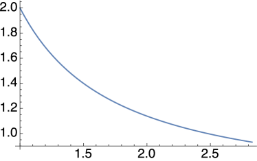 |
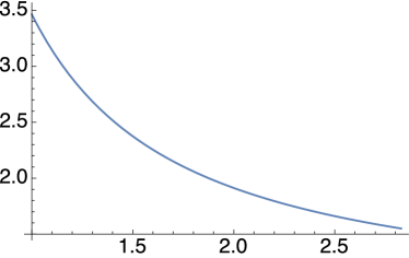 |
Figure 15 shows graphs of the width measures (LABEL:eq-width-1st-temp-der-limit-kern-scale-time-approx) and (LABEL:eq-width-2nd-temp-der-limit-kern-scale-time-approx) of the first- and second-order temporal derivatives time-causal limit kernel obtained as obtained from a scale-time approximation. As can be seen from the graphs, the width measures vary by about 30 % when the distribution parameter is varied between and . Thus, the value of the distribution parameter must be taken into explicit account when transferring the temporal scale parameter to a characteristic length estimate on the temporal axis. Notably when the distribution parameter tends to , the temporal width estimates approach the corresponding width estimates (195) and (196) of the Gaussian kernel.
Given that a temporal feature has been detected from a local maximum over temporal scales in either the first- or second-order temporal derivative of the time-causal limit kernel, if we use the behaviour of the Gaussian temporal scale-space model (195) and (196) for additional calibration of the proportionality constant of the scale estimate, we do then obtain the following estimates of the temporal duration of the corresponding temporal feature as function of the temporal scale estimate and the distribution parameter :
| (197) | ||||
| (198) | ||||
References
- (1) Adelson, E., Bergen, J.: Spatiotemporal energy models for the perception of motion. Journal of Optical Society of America A 2, 284–299 (1985)
- (2) Aertsen, A.M.H.J., Johannesma, P.I.M.: The spectro-temporal receptive field: A functional characterization of auditory neurons. Biological Cybernetics 42(2), 133–143 (1981)
- (3) Agarwal, S., Snavely, N., Simon, I., Seitz, S.M., Szeliski, R.: Building Rome in a day. In: Proc. International Conference on Computer Vision (ICCV 2009), pp. 72–79 (2009)
- (4) Alías, F., Socoró, J.C., Sevillano, X.: A review of physical and perceptual feature extraction techniques for speech, music and environmental sounds. Applied Sciences 6(5), 143 (2016)
- (5) Bay, H., Ess, A., Tuytelaars, T., van Gool, L.: Speeded up robust features (SURF). Computer Vision and Image Understanding 110(3), 346–359 (2008)
- (6) van der Berg, E.S., Reyneke, P.V., de Ridder, C.: Rotational image correlation in the Gauss-Laguerre domain. In: Third SPIE Conference on Sensors, MEMS and Electro-Optic Systems: Proc. of SPIE, vol. 9257, pp. 92,570F–1–92,570F–17 (2014)
- (7) Bicego, M., Lagorio, A., Grosso, E., Tistarelli, M.: On the use of SIFT features for face authentication. In: Proc. Computer Vision and Pattern Recognition Workshop (CVPRW 2006), p. 35 (2006)
- (8) Bosch, A., Zisserman, A., Munoz, X.: Image classification using random forests and ferns. In: Proc. International Conference on Computer Vision (ICCV 2007), pp. 1–8. Rio de Janeiro, Brazil (2007)
- (9) Bretzner, L., Laptev, I., Lindeberg, T.: Hand-gesture recognition using multi-scale colour features, hierarchical features and particle filtering. In: Proc. Face and Gesture, pp. 63–74. Washington D.C., USA (2002)
- (10) Bretzner, L., Lindeberg, T.: Feature tracking with automatic selection of spatial scales. Computer Vision and Image Understanding 71(3), 385–392 (1998)
- (11) Brown, M., Lowe, D.G.: Unsupervised 3d object recognition and reconstruction in unordered datasets. In: Proc. 3-D Digital Imaging and Modeling (3DIM 2005), pp. 56–63 (2005)
- (12) Brown, M., Lowe, D.G.: Automatic panoramic image stitching using invariant features. International Journal of Computer Vision 74(1), 59–73 (2007)
- (13) Chomat, O., de Verdiere, V., Hall, D., Crowley, J.: Local scale selection for Gaussian based description techniques. In: Proc. European Conf. on Computer Vision (ECCV 2000), Lecture Notes in Computer Science, vol. 1842, pp. I:117–133. Springer-Verlag, Dublin, Ireland (2000)
- (14) Datta, R., Joshi, D., Li, J., Wang, J.Z.: Image retrieval: Ideas, influences, and trends of the new age. ACM Computing Surveys 40(2), 5 (2008)
- (15) DeAngelis, G.C., Anzai, A.: A modern view of the classical receptive field: Linear and non-linear spatio-temporal processing by V1 neurons. In: L.M. Chalupa, J.S. Werner (eds.) The Visual Neurosciences, vol. 1, pp. 704–719. MIT Press (2004)
- (16) DeAngelis, G.C., Ohzawa, I., Freeman, R.D.: Receptive field dynamics in the central visual pathways. Trends in Neuroscience 18(10), 451–457 (1995)
- (17) Derpanis, K.G., Wildes, R.P.: Spacetime texture representation and recognition based on a spatiotemporal orientation analysis. IEEE Transactions on Pattern Analysis and Machine Intelligence 34(6), 1193–1205 (2012)
- (18) Elder, J., Zucker, S.: Local scale control for edge detection and blur estimation. IEEE Trans. Pattern Analysis and Machine Intell. 20(7), 699–716 (1998)
- (19) Ezzat, T., Bouvrie, J.V., Poggio, T.: Spectro-temporal analysis of speech using 2-D Gabor filters. In: INTERSPEECH, pp. 506–509 (2007)
- (20) Fagerström, D.: Temporal scale-spaces. International Journal of Computer Vision 2–3, 97–106 (2005)
- (21) Fleet, D.J., Langley, K.: Recursive filters for optical flow. IEEE Trans. Pattern Analysis and Machine Intell. 17(1), 61–67 (1995)
- (22) Florack, L.M.J.: Image Structure. Series in Mathematical Imaging and Vision. Springer (1997)
- (23) Frangi, A.F., J., N.W., Hoogeveen, R.M., van Walsum, T., Viergever, M.A.: Model-based quantitation of 3D magnetic resonance angiographic images. IEEE Trans. on Medical Imaging 18(10), 946–956 (2000)
- (24) Gårding, J., Lindeberg, T.: Direct computation of shape cues using scale-adapted spatial derivative operators. International Journal of Computer Vision 17(2), 163–191 (1996)
- (25) Guichard, F.: A morphological, affine, and Galilean invariant scale-space for movies. IEEE Trans. Image Processing 7(3), 444–456 (1998)
- (26) ter Haar Romeny, B.: Front-End Vision and Multi-Scale Image Analysis. Springer (2003)
- (27) ter Haar Romeny, B., Florack, L., Nielsen, M.: Scale-time kernels and models. In: Proc. Int. Conf. Scale-Space and Morphology in Computer Vision (Scale-Space’01), Springer Lecture Notes in Computer Science. Springer, Vancouver, Canada (2001)
- (28) Hall, D., de Verdiere, V., Crowley, J.: Object recognition using coloured receptive fields. In: Proc. European Conf. on Computer Vision (ECCV 2000), Springer Lecture Notes in Computer Science, vol. 1842, pp. I:164–177. Springer, Dublin, Ireland (2000)
- (29) Han, Z., Xu, Z., Zhu, S.C.: Video primal sketch: A unified middle-level representation for video. Journal of Mathematical Imaging and Vision 53(2), 151–170 (2015)
- (30) Hartley, R., Zisserman, A.: Multiple View Geometry in Computer Vision. Cambridge University Press (2004). Second Edition
- (31) Hassner, T., Mayzels, V., Zelnik-Manor, L.: On SIFTs and their scales. In: Proc. Computer Vision and Pattern Recognition (CVPR 2012), pp. 1522–1528. Providence, Rhode Island (2012)
- (32) Heckmann, M., Domont, X., Joublin, F., Goerick, C.: A hierarchical framework for spectro-temporal feature extraction. Speech Communication 53(5), 736–752 (2011)
- (33) Hubel, D.H., Wiesel, T.N.: Receptive fields of single neurones in the cat’s striate cortex. J Physiol 147, 226–238 (1959)
- (34) Hubel, D.H., Wiesel, T.N.: Brain and Visual Perception: The Story of a 25-Year Collaboration. Oxford University Press (2005)
- (35) Iijima, T.: Observation theory of two-dimensional visual patterns. Tech. rep., Papers of Technical Group on Automata and Automatic Control, IECE, Japan (1962)
- (36) J. Mutch, J., Lowe, D.G.: Object class recognition and localization using sparse features with limited receptive fields. International Journal of Computer Vision 80(1), 45–57 (2008)
- (37) Jacobs, N., Pless, R.: Time scales in video surveillance. IEEE Transactions on Circuits and Systems for Video Technology 18(8), 1106–1113 (2008)
- (38) Jaimes, A., Sebe, N.: Multimodal human–computer interaction: A survey. Computer Vision and Image Understanding 108(1), 116–134 (2007)
- (39) Jhuang, H., Serre, T., Wolf, L., Poggio, T.: A biologically inspired system for action recognition. In: International Conference on Computer Vision (ICCV’07), pp. 1–8 (2007)
- (40) Kadir, T., Brady, M.: Saliency, scale and image description. International Journal of Computer Vision 45(2), 83–105 (2001)
- (41) Kang, Y., Morooka, K., Nagahashi, H.: Scale invariant texture analysis using multi-scale local autocorrelation features. In: Proc. Scale Space and PDE Methods in Computer Vision (Scale-Space’05), Springer Lecture Notes in Computer Science, vol. 3459, pp. 363–373. Springer (2005)
- (42) Karlin, S.: Total Positivity. Stanford Univ. Press (1968)
- (43) Kläser, A., Marszalek, M., Schmid, C.: A spatio-temporal descriptor based on 3D-gradients. In: Proc. British Machine Vision Conf. Leeds, U.K. (2008)
- (44) Kleinschmidt, M.: Methods for capturing spectro-temporal modulations in automatic speech recognition. Acta Acustica united with Acustica 88(3), 416–422 (2002)
- (45) Koenderink, J.J.: The structure of images. Biological Cybernetics 50, 363–370 (1984)
- (46) Koenderink, J.J.: Scale-time. Biological Cybernetics 58, 159–162 (1988)
- (47) Koenderink, J.J., van Doorn, A.J.: Generic neighborhood operators. IEEE Trans. Pattern Analysis and Machine Intell. 14(6), 597–605 (1992)
- (48) Krissian, K., Malandain, G., Ayache, N., Vaillant, R., Trousset, Y.: Model-based detection of tubular structures in 3D images. Computer Vision and Image Understanding 80(2), 130–171 (2000)
- (49) Laptev, I., Caputo, B., Schuldt, C., Lindeberg, T.: Local velocity-adapted motion events for spatio-temporal recognition. Computer Vision and Image Understanding 108, 207–229 (2007)
- (50) Laptev, I., Lindeberg, T.: Space-time interest points. In: Proc. Int. Conf. on Computer Vision (ICCV 2003), pp. 432–439. Nice, France (2003)
- (51) Laptev, I., Lindeberg, T.: Local descriptors for spatio-temporal recognition. In: Proc. ECCV’04 Workshop on Spatial Coherence for Visual Motion Analysis, Springer Lecture Notes in Computer Science, vol. 3667, pp. 91–103. Prague, Czech Republic (2004)
- (52) Larsen, A.B.L., Darkner, S., Dahl, A.L., Pedersen, K.S.: Jet-based local image descriptors. In: Proc. European Conference on Computer Vision (ECCV 2012), Springer Lecture Notes in Computer Science, vol. 7574, pp. III:638–650. Springer (2012)
- (53) Lazebnik, S., Schmid, C., Ponce, J.: A sparse texture representation using local affine regions. IEEE Trans. Pattern Analysis and Machine Intell. 27(8), 1265–1278 (2005)
- (54) Lew, M.S., Sebe, N., Djeraba, C., Jain, R.: Content-based multimedia information retrieval: State of the art and challenges. ACM Trans. on Multimedia Computing, Communications, and Applications 2(1), 1–19 (2006)
- (55) Li, S.Z. (ed.): Encyclopedia of Biometrics. Springer Science & Business Media (2009)
- (56) Li, Y., Tax, D.M.J., Loog, M.: Supervised scale-invariant segmentation (and detection). In: Proc. Scale Space and Variational Methods in Computer Vision (SSVM 2011), Springer Lecture Notes in Computer Science, vol. 6667, pp. 350–361. Springer, Ein Gedi, Israel (2012)
- (57) Lindeberg, T.: Scale-space for discrete signals. IEEE Trans. Pattern Analysis and Machine Intell. 12(3), 234–254 (1990)
- (58) Lindeberg, T.: Discrete derivative approximations with scale-space properties: A basis for low-level feature extraction. Journal of Mathematical Imaging and Vision 3(4), 349–376 (1993)
- (59) Lindeberg, T.: Effective scale: A natural unit for measuring scale-space lifetime. IEEE Trans. Pattern Analysis and Machine Intell. 15(10), 1068–1074 (1993)
- (60) Lindeberg, T.: On scale selection for differential operators. In: Proc. 8th Scandinavian Conf. on Image Analysis (SCIA’93), pp. 857–866. Norwegian Society for Image Processing and Pattern Recognition, Tromsø, Norway (1993)
- (61) Lindeberg, T.: Scale-Space Theory in Computer Vision. Springer (1993)
- (62) Lindeberg, T.: Scale-space theory: A basic tool for analysing structures at different scales. Journal of Applied Statistics 21(2), 225–270 (1994). Also available from http://www.csc.kth.se/tony/abstracts/Lin94-SI-abstract.html
- (63) Lindeberg, T.: Linear spatio-temporal scale-space. In: B.M. ter Haar Romeny, L.M.J. Florack, J.J. Koenderink, M.A. Viergever (eds.) Proc. International Conference on Scale-Space Theory in Computer Vision (Scale-Space’97), Springer Lecture Notes in Computer Science, vol. 1252, pp. 113–127. Springer, Utrecht, The Netherlands (1997)
- (64) Lindeberg, T.: On automatic selection of temporal scales in time-casual scale-space. In: G. Sommer, J.J. Koenderink (eds.) Proc. AFPAC’97: Algebraic Frames for the Perception-Action Cycle, Springer Lecture Notes in Computer Science, vol. 1315, pp. 94–113. Kiel, Germany (1997)
- (65) Lindeberg, T.: Edge detection and ridge detection with automatic scale selection. International Journal of Computer Vision 30(2), 117–154 (1998)
- (66) Lindeberg, T.: Feature detection with automatic scale selection. International Journal of Computer Vision 30(2), 77–116 (1998)
- (67) Lindeberg, T.: A scale selection principle for estimating image deformations. Image and Vision Computing 16(14), 961–977 (1998)
- (68) Lindeberg, T.: Principles for automatic scale selection. In: Handbook on Computer Vision and Applications, pp. 239–274. Academic Press, Boston, USA (1999). Also available from http://www.csc.kth.se/cvap/abstracts/cvap222.html
- (69) Lindeberg, T.: Linear spatio-temporal scale-space. Tech. Rep. ISRN KTH/NA/P–01/22–SE, Dept. of Numerical Analysis and Computer Science, KTH (2001). Available from http://www.csc.kth.se/cvap/abstracts/cvap257.html
- (70) Lindeberg, T.: Generalized Gaussian scale-space axiomatics comprising linear scale-space, affine scale-space and spatio-temporal scale-space. Journal of Mathematical Imaging and Vision 40(1), 36–81 (2011)
- (71) Lindeberg, T.: Scale invariant feature transform. Scholarpedia 7(5), 10,491 (2012)
- (72) Lindeberg, T.: A computational theory of visual receptive fields. Biological Cybernetics 107(6), 589–635 (2013)
- (73) Lindeberg, T.: Invariance of visual operations at the level of receptive fields. PLOS ONE 8(7), e66,990 (2013)
- (74) Lindeberg, T.: Scale selection properties of generalized scale-space interest point detectors. Journal of Mathematical Imaging and Vision 46(2), 177–210 (2013)
- (75) Lindeberg, T.: Scale selection. In: K. Ikeuchi (ed.) Computer Vision: A Reference Guide, pp. 701–713. Springer (2014)
- (76) Lindeberg, T.: Image matching using generalized scale-space interest points. Journal of Mathematical Imaging and Vision 52(1), 3–36 (2015)
- (77) Lindeberg, T.: Separable time-causal and time-recursive spatio-temporal receptive fields. In: Proc. Scale-Space and Variational Methods for Computer Vision (SSVM 2015), Lecture Notes in Computer Science, vol. 9087, pp. 90–102. Springer (2015)
- (78) Lindeberg, T.: Time-causal and time-recursive spatio-temporal receptive fields. Journal of Mathematical Imaging and Vision 55(1), 50–88 (2016)
- (79) Lindeberg, T.: Spatio-temporal scale selection in video data. In preparation (2017)
- (80) Lindeberg, T., Bretzner, L.: Real-time scale selection in hybrid multi-scale representations. In: L. Griffin, M. Lillholm (eds.) Proc. Scale-Space Methods in Computer Vision (Scale-Space’03), Springer Lecture Notes in Computer Science, vol. 2695, pp. 148–163. Springer, Isle of Skye, Scotland (2003)
- (81) Lindeberg, T., Fagerström, D.: Scale-space with causal time direction. In: Proc. European Conf. on Computer Vision (ECCV’96), Springer Lecture Notes in Computer Science, vol. 1064, pp. 229–240. Cambridge, UK (1996)
- (82) Lindeberg, T., Friberg, A.: Idealized computational models of auditory receptive fields. PLOS ONE 10(3), e0119,032:1–58 (2015)
- (83) Lindeberg, T., Friberg, A.: Scale-space theory for auditory signals. In: Proc. Scale-Space and Variational Methods for Computer Vision (SSVM 2015), Lecture Notes in Computer Science, vol. 9087, pp. 3–15. Springer (2015)
- (84) Lindeberg, T., Gårding, J.: Shape from texture from a multi-scale perspective. In: T.S.H. H.-H. Nagel, Y. Shirai (eds.) Proc. Int. Conf. on Computer Vision (ICCV’93), pp. 683–691. IEEE Computer Society Press, Berlin, Germany (1993)
- (85) Lindeberg, T., Gårding, J.: Shape-adapted smoothing in estimation of 3-D depth cues from affine distortions of local 2-D structure. Image and Vision Computing 15, 415–434 (1997)
- (86) Liu, C., Yuen, J., Torralba, A.: SIFT flow: Dense correspondence across scenes and its applications. IEEE Transactions on Pattern Analysis and Machine Intelligence 33(5), 978–994 (2011)
- (87) Liu, X.M., Wang, C., Yao, H., Zhang, L.: The scale of edges. In: Proc. Computer Vision and Pattern Recognition (CVPR 2012), pp. 462–469 (2012)
- (88) Loog, M., Li, Y., Tax, D.: Maximum membership scale selection. In: Multiple Classifier Systems, Springer Lecture Notes in Computer Science, vol. 5519, pp. 468–477. Springer (2009)
- (89) Lowe, D.G.: Distinctive image features from scale-invariant keypoints. International Journal of Computer Vision 60(2), 91–110 (2004)
- (90) Mahmoodi, S.: Linear neural circuitry model for visual receptive fields. Journal of Mathematical Imaging and Vision 54(2), 1–24 (2016)
- (91) Meyer, B.T., Kollmeier, B.: Optimization and evaluation of Gabor feature sets for ASR. In: INTERSPEECH, pp. 906–909 (2008)
- (92) Mikolajczyk, K., Schmid, C.: Scale and affine invariant interest point detectors. International Journal of Computer Vision 60(1), 63–86 (2004)
- (93) Mikolajczyk, K., Tuytelaars, T., Schmid, C., Zisserman, A., Matas, J., Schaffalitzky, F., Kadir, T., van Gool, L.: A comparison of affine region detectors. International Journal of Computer Vision 65(1–2), 43–72 (2005)
- (94) Miller, L.M., Escabi, N.A., Read, H.L., Schreiner, C.: Spectrotemporal receptive fields in the lemniscal auditory thalamus and cortex. Journal of Neurophysiology 87(1), 516–527 (2001)
- (95) Mrázek, P., Navara, M.: Selection of optimal stopping time for nonlinear diffusion filtering. International Journal of Computer Vision 52(2–3), 189–203 (2003)
- (96) Negre, A., Braillon, C., Crowley, J.L., Laugier, C.: Real-time time-to-collision from variation of intrinsic scale. Experimental Robotics 39, 75–84 (2008)
- (97) Niebles, J.C., Wang, H., Fei-Fei, L.: Unsupervised learning of human action categories using spatial-temporal words. International Journal of Computer Vision 79(3), 299–318 (2008)
- (98) Paris, S.: Edge-preserving smoothing and mean-shift segmentation of video streams. In: Proc. European Conf. on Computer Vision (ECCV 2008), Springer Lecture Notes in Computer Science, pp. 460–473. Springer, Marseille, France (2008)
- (99) Patterson, R.D., Allerhand, M.H., Giguere, C.: Time-domain modeling of peripheral auditory processing: A modular architecture and a software platform. The Journal of the Acoustical Society of America 98(4), 1890–1894 (1995)
- (100) Patterson, R.D., Robinson, K., Holdsworth, J., McKeown, D., Zhang, C., Allerhand, M.: Complex sounds and auditory images. Auditory Physiology and Perception 83, 429–446 (1992)
- (101) Poppe, R.: A survey on vision-based human action recognition. Image and Vision Computing 28(6), 976–990 (2010)
- (102) Porta, M.: Vision-based user interfaces: Methods and applications. International Journal of Human-Computer Studies 57, 27–73 (2002)
- (103) Rivero-Moreno, C.J., Bres, S.: Spatio-temporal primitive extraction using Hermite and Laguerre filters for early vision video indexing. In: Image Analysis and Recognition, Springer Lecture Notes in Computer Science, vol. 3211, pp. 825–832 (2004)
- (104) Rothganger, F., Lazebnik, S., Schmid, C., Ponce, J.: 3D object modeling and recognition using local affine-invariant image descriptors and multi-view spatial constraints. International Journal of Computer Vision 66(3), 231–259 (2006)
- (105) van de Sande, K.E.A., Gevers, T., Snoek, C.G.M.: Evaluating color descriptors for object and scene recognition. IEEE Trans. Pattern Analysis and Machine Intell. 32(9), 1582–1596 (2010)
- (106) Sato, Y., Nakajima, S., Shiraga, N., Atsumi, H., Yoshida, S., Koller, T., Gerig, G., Kikinis, R.: 3D multi-scale line filter for segmentation and visualization of curvilinear structures in medical images. Medical Image Analysis 2(2), 143–168 (1998)
- (107) Schlute, R., Bezrukov, L., Wagner, H., Ney, H.: Gammatone features and feature combination for large vocabulary speech recognition. In: IEEE Int. Conf. on Acoustics, Speech and Signal Processing (ICASSP’07), vol. IV, pp. 649–652 (2007)
- (108) Schoenberg, I.J.: On Pòlya frequency functions. ii. Variation-diminishing integral operators of the convolution type. Acta Sci. Math. (Szeged) 12, 97–106 (1950)
- (109) Schoenberg, I.J.: I. J. Schoenberg Selected Papers, vol. 2. Springer (1988). Edited by C. de Boor
- (110) Se, S., Lowe, D.G., Little, J.J.: Vision-based global localization and mapping for mobile robots. IEEE Transactions on Robotics 21(3), 364–375 (2005)
- (111) Shabani, A.H., Clausi, D.A., Zelek, J.S.: Improved spatio-temporal salient feature detection for action recognition. In: British Machine Vision Conference (BMVC’11), pp. 1–12. Dundee, U.K. (2011)
- (112) Shao, L., Mattivi, R.: Feature detector and descriptor evaluation in human action recognition. In: Proc. ACM Int. Conf. on Image and Video Retrieval (CIVR’10), pp. 477–484. Xian, China (2010)
- (113) Siciliano, B., Khatib, O. (eds.): Springer Handbook of Robotics. Springer Science & Business Media (2008)
- (114) Sporring, J., Colios, C.J., Trahanias, P.E.: Generalized scale selection. In: Proc. Int. Conf. on Image Processing (ICIP’00), pp. 920–923. Vancouver, Canada (2000)
- (115) Surya, P.V.B., Vorotnikov, D., Pelapur, R., Jose, S., Seetharaman, G., Palaniappan, K.: Multiscale Tikhonov-total variation image restoration using spatially varying edge coherence exponent. IEEE Transactions on Image Processing 24(12), 5220–5235 (2015)
- (116) Tuytelaars, T., van Gool, L.: Matching widely separated views based on affine invariant regions. International Journal of Computer Vision 59(1), 61–85 (2004)
- (117) Tuytelaars, T., Mikolajczyk, K.: A Survey on Local Invariant Features, Foundations and Trends in Computer Graphics and Vision, vol. 3(3). Now Publishers (2008)
- (118) Wang, H., Ullah, M.M., Kläser, A., Laptev, I., Schmid, C.: Evaluation of local spatio-temporal features for action recognition. In: Proc. British Machine Vision Conference (BMVC 2009). London, U.K. (2009)
- (119) Wang, L., Qiao, Y., Tang, X.: Action recognition with trajectory-pooled deep-convolutional descriptors. In: IEEE Conference on Computer Vision and Pattern Recognition (CVPR 2015), pp. 4305–4314 (2015)
- (120) Weinland, D., Ronfard, R., Boyer, E.: A survey of vision-based methods for action representation, segmentation and recognition. Computer Vision and Image Understanding 115(2), 224–241 (2011)
- (121) Willems, G., Tuytelaars, T., van Gool, L.: An efficient dense and scale-invariant spatio-temporal interest point detector. In: Proc. European Conf. on Computer Vision (ECCV 2008), Springer Lecture Notes in Computer Science, vol. 5303, pp. 650–663. Marseille, France (2008)
- (122) Witkin, A.P.: Scale-space filtering. In: Proc. 8th Int. Joint Conf. Art. Intell., pp. 1019–1022. Karlsruhe, Germany (1983)
- (123) Wu, Q., Zhang, L., Shi, G.: Robust multifactor speech feature extraction based on Gabor analysis. IEEE Trans. on Audio, Speech, and Language Processing 19(4), 927–936 (2011)
- (124) Zelnik-Manor, L., Irani, M.: Event-based analysis of video. In: Proc. Computer Vision and Pattern Recognition (CVPR’01), pp. II:123–130 (2001)
![[Uncaptioned image]](/html/1701.05088/assets/x59.png)
Tony Lindeberg is a Professor of Computer Science at KTH Royal Institute of Technology in Stockholm, Sweden. He was born in Stockholm in 1964, received his MSc degree in 1987, his PhD degree in 1991, became docent in 1996, and was appointed professor in 2000. He was a Research Fellow at the Royal Swedish Academy of Sciences between 2000 and 2010.
His research interests in computer vision relate to scale-space representation, image features, object recognition, spatio-temporal recognition, focus-of-attention and computational modelling of biological vision. He has developed theories and methodologies for continuous and discrete scale-space representation, visual and auditory receptive fields, detection of salient image structures, automatic scale selection, scale-invariant image features, affine invariant features, affine and Galilean normalization, temporal, spatio-temporal and spectro-temporal scale-space concepts as well as spatial and spatio-temporal image descriptors for image-based recognition. He has also worked on topics in medical image analysis and gesture recognition. He is author of the book Scale-Space Theory in Computer Vision.