POD reduced order modeling for evolution equations utilizing arbitrary finite element discretizations

Carmen Gräßle and Michael Hinze
Abstract

The main focus of the present work is the inclusion of spatial adaptivity for the snapshot computation in the offline phase of model order reduction utilizing Proper Orthogonal Decomposition (POD-MOR) for nonlinear parabolic evolution problems. We consider snapshots which live in different finite element spaces, which means in a fully discrete setting that the snapshots are vectors of different length. From a numerical point of view, this leads to the problem that the usual POD procedure which utilizes a singular value decomposition of the snapshot matrix, cannot be carried out. In order to overcome this problem, we here construct the POD model / basis using the eigensystem of the correlation matrix (snapshot gramian), which is motivated from a continuous perspective and is set up explicitly e.g. without the necessity of interpolating snapshots into a common finite element space. It is an advantage of this approach that the assembling of the matrix only requires the evaluation of inner products of snapshots in a common Hilbert space. This allows a great flexibility concerning the spatial discretization of the snapshots. The analysis for the error between the resulting POD solution and the true solution reveals that the accuracy of the reduced order solution can be estimated by the spatial and temporal discretization error as well as the POD error. Finally, to illustrate the feasibility our approach, we present a test case of the Cahn-Hilliard system utilizing hh-adapted hierarchical meshes and two settings of a linear heat equation using nested and non-nested grids.

Keywords and phrases: Model Order Reduction, Proper Orthogonal Decomposition, Adaptive Finite Element Discretization, Partial Differential Equation, Evolution Equations
Acknowlegdements: We like to thank Christian Kahle for providing many C++ libraries which we could use for the coding. The authors gratefully acknowledge the financial support by the Deutsche Forschungsgemeinschaft through the priority program SPP1962 entitled “Non-smooth and Complementarity-based Distributed Parameter Systems: Simulation and Hierarchical Optimization”.

1 Introduction

For many problem settings, model order reduction utilizing Proper Orthogonal Decomposition (POD) has proven to be a powerful tool in order to reduce large scale systems to surrogate models of low dimension while preserving a good approximation quality. The range of applications of POD model order reduction (POD-MOR) comprises a broad scope, including (amongst others) linear and nonlinear parabolic equations [29], optimal control of partial differential equations [20, 50, 28, 26, 3] and fluid dynamics [35, 23, 33]. A general introduction to POD and reduced order modeling can be found in [25, 42, 51], for example. The key idea of the POD technique is to apply a Galerkin ansatz, in which the ansatz functions, i.e. the POD basis functions, contain information about the underlying dynamical system. Following the approach of snapshot based POD in [48], the system information is retrieved from snapshots of the solution trajectory at several time instances, which are generated in a simulation.
In practice, many simulations require adaptive strategies for the spatial discretization in order to be implementable. For example, in the simulation of Cahn-Hilliard systems based on diffuse interface approaches, many degrees of freedom are required at the interfacial regions in order to well resemble the steep gradients, whereas in the pure phases only little numbers of degrees of freedom are needed, see [22] for example. Utilizing a uniform mesh for such problems would drastically enlarge the computational effort and storage problems would occur.
In [11] adaptive finite element methods and POD reduced order modeling are considered as two different techniques in order to reduce the complexity of the numerical solution of optimal control problems. The combination of both approaches contains a major challenge. The inclusion of spatial adaptivity in the context of model reduction means, in a discrete formulation, that the snapshots at each time instance may have different lengths due to their different spatial resolutions. For this reason, the snapshot matrix cannot be set up directly and the usual POD procedure cannot be carried out. In this paper, we consider the combination of adaptive finite element snapshots with POD model order reduction. Our perspective is based on the continuous setting, which allows us to derive a reduced order model utilizing snapshots which only need to lie in a common Hilbert space. Thus, for the actual numerical implementation, this allows us to use spatially adapted finite element snapshots or even a blend of snapshots stemming from different discretization schemes.
The inclusion of spatial adaptivity in the POD framework is advantageous from two perspectives: on the one hand, the use of adaptive finite elements for snapshot generation can remarkably reduce the offline computation time in comparison to the use of a uniform mesh with resolution of the finest level of the adaptive grids. On the other hand, we expect to speed up the computations when solving the POD surrogate model in contrast to utilizing adaptive finite elements, since we solve POD reduced systems of low order.
In order to overcome the difficulties arising from combining POD with adaptive finite elements, different concepts are proposed. In [18], the use of dynamically adaptive meshes is combined with POD-MOR for an unstructured ocean model. A fixed reference mesh is utilized, onto which the spatial adaptive snapshots are interpolated. This allows snapshots of the same lengths at each time level and the usual POD procedure can then be performed on this fixed reference mesh. In [31, Ch. 2.4.3] an interpolation approach is outlined. The idea is to interpolate given snapshots of arbitrary spatial discretizations by (piecewise) polynomials. For the fully discrete POD setting, the spatial discretization points are chosen appropriately for the numerical integration of the polynomials. In the context of reduced basis methods, adaptive wavelet discretizations are used in [5] in the offline snapshot computation phase. In [54], a reduced basis method is developed which is certified by a residual bound relative to the infinite-dimensional weak solution. Different adaptive strategies are considered for both the finite element and the reduced basis level. Furthermore, in [24] three numerical concepts to treat the moving free boundary for the calculation of the snapshots are compared: first a Landau-type transformation, second a control volume approach and third a moving mesh approach. In contrary to the first two concepts, the number of grid points in the moving mesh approach (r-adaptivity) is kept fixed, but they are moved according to the evolution of the free boundary. POD is applicable with only minor modifications. Recently and in parallel to our work, the combination of POD model reduction with adaptive finite element snapshots is realized in [49] by constructing common finite element spaces. Two options are considered: either all snapshots are expressed in terms of a common finite element basis or pairs of snapshots are expressed in terms of a common finite element basis of these pairs. Moreover, error statements for a parametrized elliptic boundary value problem are proved. In the numerical examples, hh-adaptive finite elements with fixed polynomial degree are utilized.
The aim of this work is to derive a POD reduced order model for a general semilinear evolution equation which can be set up and solved for arbitrary finite element discretizations without the necessity of e.g. using interpolation with respect to the spatial variable. This approach is motivated from a continuous perspective, where snapshots from different finite element spaces belong to a same Hilbert space. The assembly of the snapshot matrix can be avoided by directly setting up an eigenvalue problem for which we only need the calculation of the inner product of the finite element ansatz functions. This can be computed for arbitrary finite element discretizations and suffices to set up a POD-ROM. We provide an algorithm which enables the evaluation of the inner products of snapshots stemming from arbitrary finite element discretizations. In the numerical examples, the method is demonstrated for both hh-adapted snapshots and snapshots with non-nested meshes. Moreover, the treatment of the nonlinearity is discussed.
The paper is organized as follows: the general problem setting of an abstract semilinear parabolic evolution problem is described in Section 2. We recall the POD method in real Hilbert spaces in Section 3 and set up a POD eigenvalue problem which can be assembled for any finite element discretization. The POD reduced order model for arbitrary finite element discretizations is discussed in Section 4. In order to validate the quality of the POD solution, we investigate the error between the POD solution and the true solution in Section 5. Numerical examples are presented in Section 6 to illustrate our approach.

2 Abstract semilinear parabolic evolution problem

2.1 Problem setting

Let us specify the abstract semilinear parabolic evolution problem which we consider in the following. Let (V,,V)𝑉subscript𝑉(V,\langle\cdot,\cdot\rangle_{V}) and (H,,H)𝐻subscript𝐻(H,\langle\cdot,\cdot\rangle_{H}) be real separable Hilbert spaces such that there exists a dense and continuous embedding VH𝑉𝐻V\hookrightarrow H. The dual space Hsuperscript𝐻H^{\prime} can be identified with H𝐻H by the Riesz representation theorem and the Gelfand triple (V,H,V)𝑉𝐻superscript𝑉(V,H,V^{\prime}) is formed by VH=HV𝑉𝐻superscript𝐻superscript𝑉V\hookrightarrow H=H^{\prime}\hookrightarrow V^{\prime}. Since V𝑉V is continuously embedded in H𝐻H, there exists a constant cv>0subscript𝑐𝑣0c_{v}>0 such that

vH2cvvV2 for all vV.formulae-sequencesuperscriptsubscriptnorm𝑣𝐻2subscript𝑐𝑣superscriptsubscriptnorm𝑣𝑉2 for all 𝑣𝑉\|v\|_{H}^{2}\leq c_{v}\|v\|_{V}^{2}\quad\text{ for all }v\in V. (1)

For a given symmetric, V𝑉V-elliptic bilinear form a:V×V:𝑎𝑉𝑉a:V\times V\to\mathbb{R}, we assume boundedness, i.e.

β>0:|a(u,v)|βuVvV for all u,vV\exists\beta>0:\quad|a(u,v)|\leq\beta\|u\|_{V}\|v\|_{V}\quad\text{ for all }u,v\in V (2)

and coercivity, i.e.

κ>0:a(u,u)κuV2 for all uV.\exists\kappa>0:\quad a(u,u)\geq\kappa\|u\|_{V}^{2}\quad\text{ for all }u\in V.

Let 𝒜:VV:𝒜𝑉superscript𝑉\mathcal{A}:V\to V^{\prime} be the bounded linear operator associated with the bilinear form a𝑎a, i.e. 𝒜(V,V)𝒜𝑉superscript𝑉\mathcal{A}\in\mathcal{L}(V,V^{\prime}) and

a(u,v)=𝒜u,vV,V=u𝒜vV,Vfor all u,vV,formulae-sequence𝑎𝑢𝑣subscript𝒜𝑢𝑣superscript𝑉𝑉subscriptdelimited-⟨⟩𝑢superscript𝒜𝑣𝑉superscript𝑉for all 𝑢𝑣𝑉a(u,v)=\langle\mathcal{A}u,v\rangle_{V^{\prime},V}=\langle u\mathcal{A}^{\star}v\rangle_{V,V^{\prime}}\quad\text{for all }u,v\in V,

where ,V,Vsubscriptsuperscript𝑉𝑉\langle\cdot,\cdot\rangle_{V^{\prime},V} denotes the dual pairing of Vsuperscript𝑉V^{\prime} and V𝑉V. Moreover, we denote by 𝒩:VV:𝒩𝑉superscript𝑉\mathcal{N}:V\to V^{\prime} a nonlinear operator. We are concerned with the following Cauchy problem for a semilinear evolution problem. Let T>0𝑇0T>0 be a fixed end time. For a given initial function gH𝑔𝐻g\in H and external force fL2(0,T;V)𝑓superscript𝐿20𝑇superscript𝑉f\in L^{2}(0,T;V^{\prime}) we consider the problem: find yW(0,T):={vL2(0,T;V),vtL2(0,T;V)}𝑦𝑊0𝑇assignformulae-sequence𝑣superscript𝐿20𝑇𝑉subscript𝑣𝑡superscript𝐿20𝑇superscript𝑉y\in W(0,T):=\{v\in L^{2}(0,T;V),v_{t}\in L^{2}(0,T;V^{\prime})\} with

{ddty(t),vH+a(y(t),v)+𝒩(y(t)),vV,V=f(t),vV,V,y(0),vH=g,vH,cases𝑑𝑑𝑡subscript𝑦𝑡𝑣𝐻𝑎𝑦𝑡𝑣subscript𝒩𝑦𝑡𝑣superscript𝑉𝑉subscript𝑓𝑡𝑣superscript𝑉𝑉subscript𝑦0𝑣𝐻subscript𝑔𝑣𝐻\left\{\begin{array}[]{rcl}\frac{d}{dt}\langle y(t),v\rangle_{H}+a(y(t),v)+\langle\mathcal{N}(y(t)),v\rangle_{V^{\prime},V}&=&\langle f(t),v\rangle_{V^{\prime},V},\\ \langle y(0),v\rangle_{H}&=&\langle g,v\rangle_{H},\\ \end{array}\right. (3)

for all vV𝑣𝑉v\in V and for almost all t(0,T]𝑡0𝑇t\in(0,T]. Note that it holds ddty(t),vH=y(t),vV,V𝑑𝑑𝑡subscript𝑦𝑡𝑣𝐻subscriptsuperscript𝑦𝑡𝑣superscript𝑉𝑉\frac{d}{dt}\langle y(t),v\rangle_{H}=\langle y^{\prime}(t),v\rangle_{V^{\prime},V} for all yL2(0,T;V)𝑦superscript𝐿20𝑇𝑉y\in L^{2}(0,T;V) with yL2(0,T;V)superscript𝑦superscript𝐿20𝑇superscript𝑉y^{\prime}\in L^{2}(0,T;V^{\prime}) and all vV𝑣𝑉v\in V in the sense of distributions in (0,T)0𝑇(0,T).

Assumption 2.1. For every fL2(0,T;V)𝑓superscript𝐿20𝑇superscript𝑉f\in L^{2}(0,T;V^{\prime}) and gH𝑔𝐻g\in H there exists a unique weak solution of (3) with

yL2(0,T;V)C([0,T];H)H1(0,T;V).𝑦superscript𝐿20𝑇𝑉𝐶0𝑇𝐻superscript𝐻10𝑇superscript𝑉y\in L^{2}(0,T;V)\cap C([0,T];H)\cap H^{1}(0,T;V^{\prime}).

Remark 2.2. Under monotonicity, boundedness and Lipschitz continuity assumptions on the nonlinear operator 𝒩𝒩\mathcal{N}, existence and uniqueness results for a general abstract evolution equation of type (3) are proved in [53, Th. 4.1] or [39, Ch. 6], for example.

Example 2.3 (Semilinear heat equation). Let Ωk,k{2,3}formulae-sequenceΩsuperscript𝑘𝑘23\Omega\subset\mathbb{R}^{k},k\in\{2,3\} be a bounded open domain with Lipschitz continuous boundary ΩΩ\partial\Omega and let T>0𝑇0T>0 be a fixed end time. We set Q:=(0,T)×Ωassign𝑄0𝑇ΩQ:=(0,T)\times\Omega and Σ:=(0,T)×ΩassignΣ0𝑇Ω\Sigma:=(0,T)\times\partial\Omega and c0𝑐0c\geq 0. For a given forcing term fL2(Q)𝑓superscript𝐿2𝑄f\in L^{2}(Q) and initial condition gL2(Ω)𝑔superscript𝐿2Ωg\in L^{2}(\Omega), we consider the semilinear heat equation with homogeneous Dirichlet boundary condition:

{yt(t,x)Δy(t,x)+cy3(t,x)=f(t,x)in Q,y(t,x)=0on Σ,y(0,x)=g(x)in Ω.casessubscript𝑦𝑡𝑡𝑥Δ𝑦𝑡𝑥𝑐superscript𝑦3𝑡𝑥𝑓𝑡𝑥in 𝑄𝑦𝑡𝑥0on Σ𝑦0𝑥𝑔𝑥in Ω\left\{\begin{array}[]{r c l l}y_{t}(t,x)-\Delta y(t,x)+cy^{3}(t,x)&=&f(t,x)&\text{in }Q,\\ y(t,x)&=&0&\text{on }\Sigma,\\ y(0,x)&=&g(x)&\text{in }\Omega.\end{array}\right. (4)

The existence of a unique solution to (4) is proved in [43], for example. We can write (4) as an abstract evolution problem of type (3) by deriving a variational formulation for (4) with V=H01(Ω)𝑉superscriptsubscript𝐻01ΩV=H_{0}^{1}(\Omega) as the space of test functions, H=L2(Ω)𝐻superscript𝐿2ΩH=L^{2}(\Omega) and integrating over the space ΩΩ\Omega. The bilinear form a:V×V:𝑎𝑉𝑉a:V\times V\to\mathbb{R} is introduced by

a(u,v)=Ωuv𝑎𝑢𝑣subscriptΩ𝑢𝑣a(u,v)=\int_{\Omega}\nabla u\cdot\nabla v

and the operator 𝒩:VV:𝒩𝑉superscript𝑉\mathcal{N}:V\to V^{\prime} is defined as 𝒩(y)=y3𝒩𝑦superscript𝑦3\mathcal{N}(y)=y^{3}. For c0𝑐0c\equiv 0, the heat equation (4) is linear.

Example 2.4 (Cahn-Hilliard equations). Let Ω,T,QΩ𝑇𝑄\Omega,T,Q and ΣΣ\Sigma be defined as in Example 2.3. The Cahn-Hilliard system was proposed in [14] as a model for phase separation in binary alloys. Introducing the chemical potential w𝑤w, the Cahn-Hilliard equations can be formulated in the common setting as a coupled system for the phase field c𝑐c and the chemical potential w𝑤w:

{ct(t,x)+yc(t,x)=mΔw(t,x)in Q,w(t,x)=σεΔc(t,x)+σεW(c(t,x))in Q,c(t,x)νΩ=w(t,x)νΩ=0on Σ,c(0,x)=c0(x)in Ω.casessubscript𝑐𝑡𝑡𝑥𝑦𝑐𝑡𝑥𝑚Δ𝑤𝑡𝑥in 𝑄𝑤𝑡𝑥𝜎𝜀Δ𝑐𝑡𝑥𝜎𝜀superscript𝑊𝑐𝑡𝑥in 𝑄𝑐𝑡𝑥subscript𝜈Ω𝑤𝑡𝑥subscript𝜈Ω0on Σ𝑐0𝑥subscript𝑐0𝑥in Ω\left\{\begin{array}[]{rcll}c_{t}(t,x)+y\cdot\nabla c(t,x)&=&m\Delta w(t,x)&\text{in }Q,\\ w(t,x)&=&-\sigma\varepsilon\Delta c(t,x)+\frac{\sigma}{\varepsilon}W^{\prime}(c(t,x))&\text{in }Q,\\ \nabla c(t,x)\cdot\nu_{\Omega}&=&\nabla w(t,x)\cdot\nu_{\Omega}=0&\text{on }\Sigma,\\ c(0,x)&=&c_{0}(x)&\text{in }\Omega.\end{array}\right. (5)

By νΩsubscript𝜈Ω\nu_{\Omega} we denote the outward normal on ΩΩ\partial\Omega, m0𝑚0m\geq 0 is a constant mobility, σ>0𝜎0\sigma>0 denotes the surface tension and 0<ε10𝜀much-less-than10<\varepsilon\ll 1 represents the interface parameter. Note that the convective term yc𝑦𝑐y\cdot\nabla c describes the transport with (constant) velocity y𝑦y. The transport term represents the coupling to the Navier-Stokes equations in the context of multiphase flow, see e.g. [21] and [2]. The phase field function c𝑐c describes the phase of a binary material with components A𝐴A and B𝐵B. It is c1𝑐1c\equiv-1 in the pure A𝐴A-phase and c+1𝑐1c\equiv+1 in the pure B𝐵B-phase. The interfacial region is described by c(1,1)𝑐11c\in(-1,1) and its thickness is finite and of order 𝒪(ε)𝒪𝜀\mathcal{O}(\varepsilon). The function W(c)𝑊𝑐W(c) is a double well potential. A typical choice for W𝑊W is the polynomial free energy function

Wp(c)=(1c2)2/4,superscript𝑊𝑝𝑐superscript1superscript𝑐224W^{p}(c)=(1-c^{2})^{2}/4, (6)

which has exactly two minimal points at c=±1𝑐plus-or-minus1c=\pm 1, i.e. at the energetically favorable state. Another choice for W𝑊W is the relaxed double obstacle free energy

Wsrel(c)=12(1c2)+s2(max(c1,0)2+min(c+1,0)2),W^{\text{rel}}_{s}(c)=\frac{1}{2}(1-c^{2})+\frac{s}{2}(\max(c-1,0)^{2}+\min(c+1,0)^{2}), (7)

with relaxation parameter s0much-greater-than𝑠0s\gg 0, which is introduced in [22] as the Moreau-Yosida relaxation of the double obstacle free energy

W(c)={12(1c2),if c[1,1],+,else. superscript𝑊𝑐cases121superscript𝑐2if 𝑐11else. W^{\infty}(c)=\begin{cases}\frac{1}{2}(1-c^{2}),&\text{if }c\in[-1,1],\\ +\infty,&\text{else. }\end{cases}

For more details on the choices for W𝑊W we refer to [1] and [9], for example. Concerning existence, uniqueness and regularity of a solution to (5), we refer to [9].

In order to derive a variational form of type (3), we write (5) as a single fourth-order parabolic equation for c𝑐c by

{ct(t,x)+yc=mΔ(σεΔc(t,x)+σεW(c(t,x)))in Q,c(t,x)νΩ=(σεΔc(t,x)+σεW(c(t,x)))νΩ=0on Σ,c(0,x)=c0(x)in Ω.casessubscript𝑐𝑡𝑡𝑥𝑦𝑐𝑚Δ𝜎𝜀Δ𝑐𝑡𝑥𝜎𝜀superscript𝑊𝑐𝑡𝑥in 𝑄𝑐𝑡𝑥subscript𝜈Ω𝜎𝜀Δ𝑐𝑡𝑥𝜎𝜀superscript𝑊𝑐𝑡𝑥subscript𝜈Ω0on Σ𝑐0𝑥subscript𝑐0𝑥in Ω\left\{\begin{array}[]{rcll}c_{t}(t,x)+y\cdot\nabla c&=&m\Delta(-\sigma\varepsilon\Delta c(t,x)+\frac{\sigma}{\varepsilon}W^{\prime}(c(t,x)))&\text{in }Q,\\ \nabla c(t,x)\cdot\nu_{\Omega}&=&\nabla(-\sigma\varepsilon\Delta c(t,x)+\frac{\sigma}{\varepsilon}W^{\prime}(c(t,x)))\cdot\nu_{\Omega}=0&\text{on }\Sigma,\\ c(0,x)&=&c_{0}(x)&\text{in }\Omega.\end{array}\right. (8)

We choose V={vH1(Ω):1|Ω|Ωv=0}𝑉conditional-set𝑣superscript𝐻1Ω1ΩsubscriptΩ𝑣0V=\{v\in H^{1}(\Omega):\frac{1}{|\Omega|}\int_{\Omega}v=0\} equipped with the inner product (u,v)V:=Ωuvassignsubscript𝑢𝑣𝑉subscriptΩ𝑢𝑣(u,v)_{V}:=\int_{\Omega}\nabla u\nabla v, so that the dual space of V𝑉V is given by V={f(H1(Ω)):f,1=0}superscript𝑉conditional-set𝑓superscriptsuperscript𝐻1Ω𝑓10V^{\prime}=\{f\in(H^{1}(\Omega))^{\prime}:\langle f,1\rangle=0\} such that VH=V𝑉𝐻superscript𝑉V\hookrightarrow H=V^{\prime} and .,.\langle.,.\rangle denotes the duality pairing. We note that (V,(.,.)V)(V,(.,.)_{V}) is a Hilbert space. We define the Vlimit-fromsuperscript𝑉V^{\prime}-inner product for f,gV𝑓𝑔superscript𝑉f,g\in V^{\prime} as (f,g)V:=Ω(Δ)1f(Δ)1g(f,g)_{V^{\prime}}:=\int_{\Omega}\nabla(-\Delta)^{-1}f\cdot\nabla(-\Delta)^{-1}g where (Δ)1superscriptΔ1(-\Delta)^{-1} denotes the inverse of the negative Laplacian with zero Neumann boundary data. Note that (f,g)V=(f,(Δ)1g)L2(Ω)=((Δ)1f,g)L2(Ω)subscript𝑓𝑔superscript𝑉subscript𝑓superscriptΔ1𝑔superscript𝐿2ΩsubscriptsuperscriptΔ1𝑓𝑔superscript𝐿2Ω(f,g)_{V^{\prime}}=(f,(-\Delta)^{-1}g)_{L^{2}(\Omega)}=((-\Delta)^{-1}f,g)_{L^{2}(\Omega)}. We introduce the bilinear form a:V×V:𝑎𝑉𝑉a:V\times V\to\mathbb{R} by

a(u,v)=σε(u,v)L2(Ω)+1m(yu,v)V𝑎𝑢𝑣𝜎𝜀subscript𝑢𝑣superscript𝐿2Ω1𝑚subscript𝑦𝑢𝑣superscript𝑉a(u,v)=\sigma\varepsilon(\nabla u,\nabla v)_{L^{2}(\Omega)}+\frac{1}{m}(y\cdot\nabla u,v)_{V^{\prime}}

and define the nonlinear operator 𝒩𝒩\mathcal{N} by 𝒩(c)=σεW(c).𝒩𝑐𝜎𝜀superscript𝑊𝑐\mathcal{N}(c)=\frac{\sigma}{\varepsilon}W^{\prime}(c). The evolution problem can be written in the form

1m(ct(t),v)V+a(c(t),v)+𝒩(c(t)),v=0vV and a.a. t(0,T].formulae-sequence1𝑚subscriptsubscript𝑐𝑡𝑡𝑣superscript𝑉𝑎𝑐𝑡𝑣𝒩𝑐𝑡𝑣0for-all𝑣𝑉 and a.a. 𝑡0𝑇\frac{1}{m}(c_{t}(t),v)_{V^{\prime}}+a(c(t),v)+\langle\mathcal{N}(c(t)),v\rangle=0\quad\forall v\in V\text{ and a.a. }t\in(0,T]. (9)

We note that this fits our abstract setting formulated in (3) with the Gelfand triple VHVV𝑉𝐻superscript𝑉superscript𝑉V\hookrightarrow H\equiv V^{\prime}\hookrightarrow V^{\prime}.

2.2 Temporal and spatial discretization

In order to solve (3) numerically, we apply the implicit Euler method for temporal discretization. Of course, other time integration schemes are possible. For a given n𝑛n\in\mathbb{N} let

0=t0<<tn=T0subscript𝑡0subscript𝑡𝑛𝑇0=t_{0}<\dotsc<t_{n}=T (10)

denote an arbitrary grid in the time interval [0,T]0𝑇[0,T] with time step sizes

Δtj:=tjtj1assignΔsubscript𝑡𝑗subscript𝑡𝑗subscript𝑡𝑗1\Delta t_{j}:=t_{j}-t_{j-1}

for j=1,,n𝑗1𝑛j=1,\dotsc,n. We set Ij=[tj1,tj]subscript𝐼𝑗subscript𝑡𝑗1subscript𝑡𝑗I_{j}=[t_{j-1},t_{j}] for each time interval j=1,,n𝑗1𝑛j=1,\dotsc,n. The resulting time-discrete system consists in finding a sequence {y¯j}j=0nVsuperscriptsubscriptsubscript¯𝑦𝑗𝑗0𝑛𝑉\{\bar{y}_{j}\}_{j=0}^{n}\subset V satisfying the following system of equations

{y¯jy¯j1Δtj,vH+a(y¯j,v)+𝒩(y¯j),vV,V=1Δtjtj1tjfj,vV,V𝑑t, for j=1,,ny¯0,vH=g,vH,casessubscriptsubscript¯𝑦𝑗subscript¯𝑦𝑗1Δsubscript𝑡𝑗𝑣𝐻𝑎subscript¯𝑦𝑗𝑣subscript𝒩subscript¯𝑦𝑗𝑣superscript𝑉𝑉1Δsubscript𝑡𝑗superscriptsubscriptsubscript𝑡𝑗1subscript𝑡𝑗subscriptsubscript𝑓𝑗𝑣superscript𝑉𝑉differential-d𝑡 for 𝑗1𝑛subscriptsubscript¯𝑦0𝑣𝐻subscript𝑔𝑣𝐻missing-subexpression\left\{\begin{array}[]{rcll}\langle\displaystyle\frac{\bar{y}_{j}-\bar{y}_{j-1}}{\Delta t_{j}},v\rangle_{H}+a(\bar{y}_{j},v)+\langle\mathcal{N}(\bar{y}_{j}),v\rangle_{V^{\prime},V}&=&\displaystyle\frac{1}{\Delta t_{j}}\int_{t_{j-1}}^{t_{j}}\langle f_{j},v\rangle_{V^{\prime},V}dt,&\text{ for }j=1,\dotsc,n\\ \langle\bar{y}_{0},v\rangle_{H}&=&\langle g,v\rangle_{H},&\\ \end{array}\right. (11)

for all vV𝑣𝑉v\in V and fjsubscript𝑓𝑗f_{j} denotes fj=f(tj)Vsubscript𝑓𝑗𝑓subscript𝑡𝑗superscript𝑉f_{j}=f(t_{j})\in V^{\prime} for j=1,,n𝑗1𝑛j=1,\cdots,n.

For the spatial discretization we utilize adaptive finite elements. At each time point tjsubscript𝑡𝑗t_{j}, j=0,,n,𝑗0𝑛j=0,\dotsc,n, we introduce a regular triangulation 𝒯jsubscript𝒯𝑗\mathcal{T}_{j} of Ω¯¯Ω\bar{\Omega} and define an Njsubscript𝑁𝑗N_{j}-dimensional conformal subspace Vjsubscript𝑉𝑗V_{j} of V𝑉V by

Vj:=span{v1j,,vNjj}Vassignsubscript𝑉𝑗spansuperscriptsubscript𝑣1𝑗superscriptsubscript𝑣subscript𝑁𝑗𝑗𝑉V_{j}:=\text{span}\{v_{1}^{j},\dotsc,v_{N_{j}}^{j}\}\subset V

with nodal basis {vij}i=1Njsuperscriptsubscriptsuperscriptsubscript𝑣𝑖𝑗𝑖1subscript𝑁𝑗\{v_{i}^{j}\}_{i=1}^{N_{j}}, i.e. vij(Pkj)=δiksuperscriptsubscript𝑣𝑖𝑗superscriptsubscript𝑃𝑘𝑗subscript𝛿𝑖𝑘v_{i}^{j}(P_{k}^{j})=\delta_{ik} for i,k=1,,Njformulae-sequence𝑖𝑘1subscript𝑁𝑗i,k=1,\dotsc,N_{j} with the nodes {Pkj}k=1Njsuperscriptsubscriptsuperscriptsubscript𝑃𝑘𝑗𝑘1subscript𝑁𝑗\{P_{k}^{j}\}_{k=1}^{N_{j}} of the underlying triangulation 𝒯jsubscript𝒯𝑗\mathcal{T}_{j}. Therefore, at each time level j=0,,n𝑗0𝑛j=0,\dotsc,n, the utilized finite element spaces {Vj}j=0nsuperscriptsubscriptsubscript𝑉𝑗𝑗0𝑛\{V_{j}\}_{j=0}^{n} can differ both in the underlying triangulation of the domain Ω¯¯Ω\bar{\Omega} and in the polynomial degree. This means that the solutions can be computed utilizing hlimit-fromh-, plimit-from𝑝p- and rlimit-from𝑟r-adaptivity, where hlimit-fromh-adaptivity denotes local refinement and coarsening of the triangulation according to certain error indicators, plimit-from𝑝p-adaptivity means increasing and decreasing the polynomial degree according to the smoothness of the solution and rlimit-from𝑟r-adaptivity, or moving mesh methods, relocates the mesh points to concentrate them in specific regions. We apply a Galerkin scheme for (11). Thus we look for a sequence {yj}j=0nsuperscriptsubscriptsubscript𝑦𝑗𝑗0𝑛\{y_{j}\}_{j=0}^{n} with yjVjsubscript𝑦𝑗subscript𝑉𝑗y_{j}\in V_{j} which fulfills

{yj𝕀jyj1Δtj,vH+a(yj,v)+𝒩(yj),vV,V=fj,vV,V, for j=1,,ny0,vH=g,vH,casessubscriptsubscript𝑦𝑗superscript𝕀𝑗subscript𝑦𝑗1Δsubscript𝑡𝑗𝑣𝐻𝑎subscript𝑦𝑗𝑣subscript𝒩subscript𝑦𝑗𝑣superscript𝑉𝑉subscriptsubscript𝑓𝑗𝑣superscript𝑉𝑉 for 𝑗1𝑛subscriptsubscript𝑦0𝑣𝐻subscript𝑔𝑣𝐻missing-subexpression\left\{\begin{array}[]{rcll}\langle\displaystyle\frac{y_{j}-\mathbb{I}^{j}y_{j-1}}{\Delta t_{j}},v\rangle_{H}+a(y_{j},v)+\langle\mathcal{N}(y_{j}),v\rangle_{V^{\prime},V}&=&\langle f_{j},v\rangle_{V^{\prime},V},&\text{ for }j=1,\dotsc,n\\ \langle y_{0},v\rangle_{H}&=&\langle g,v\rangle_{H},&\\ \end{array}\right. (12)

for all vVj𝑣subscript𝑉𝑗v\in V_{j}, where 𝕀j:C(Ω¯)Vj:superscript𝕀𝑗𝐶¯Ωsubscript𝑉𝑗\mathbb{I}^{j}:C(\bar{\Omega})\to V_{j} denotes the Lagrange interpolation. Since yjVjsubscript𝑦𝑗subscript𝑉𝑗y_{j}\in V_{j} holds, we make the Galerkin ansatz

yj=i=1Nj𝗒ijvijVjVsubscript𝑦𝑗superscriptsubscript𝑖1superscript𝑁𝑗superscriptsubscript𝗒𝑖𝑗superscriptsubscript𝑣𝑖𝑗subscript𝑉𝑗𝑉y_{j}=\displaystyle\sum_{i=1}^{N^{j}}\mathsf{y}_{i}^{j}v_{i}^{j}\in V_{j}\subset V (13)

for j=0,,n𝑗0𝑛j=0,\dotsc,n with appropriate mode coefficients {𝗒ij}i=1Njsuperscriptsubscriptsuperscriptsubscript𝗒𝑖𝑗𝑖1superscript𝑁𝑗\{\mathsf{y}_{i}^{j}\}_{i=1}^{N^{j}}.

3 POD method utilizing snapshots with arbitrary finite element discretizations

3.1 POD method in real Hilbert spaces

The aim of this work is to propose a POD-ROM which uses the correlation matrix in order to construct the POD basis and POD surrogate model and avoids the necessity of e.g. interpolating the snapshots into a common finite element space. For this reason, the POD method is explained from an infinite-dimensional perspective in this section, where we use a finite number of snapshots which lie in a common Hilbert space. The POD method in Hilbert spaces is explained in [30] and [50], for example. Here, we recall the main aspects.

Assume we are given snapshots

y0V0,,ynVnformulae-sequencesubscript𝑦0subscript𝑉0subscript𝑦𝑛subscript𝑉𝑛y_{0}\in V_{0},\dotsc,y_{n}\in V_{n}

of (3), which can be finite element samples of the solution trajectory 𝒱=span{y(t)|t[0,T]}𝒱spanconditional-set𝑦𝑡𝑡0𝑇\mathcal{V}=\text{span}\{y(t)\;|\;t\in[0,T]\} for (3) on the given timegrid {tj}j=0nsuperscriptsubscriptsubscript𝑡𝑗𝑗0𝑛\{t_{j}\}_{j=0}^{n} introduced in (10). For each time level j=0,,n𝑗0𝑛j=0,\dotsc,n the snapshots belong to different subspaces V0,,VnVsubscript𝑉0subscript𝑉𝑛𝑉V_{0},\dotsc,V_{n}\subset V. Note that by construction we have 𝒱:=span{yj}j=0nVassign𝒱spansuperscriptsubscriptsubscript𝑦𝑗𝑗0𝑛𝑉\mathcal{V}:=\text{span}\{y_{j}\}_{j=0}^{n}\subset V.

The idea of the POD method is to describe the space 𝒱𝒱\mathcal{V} by means of few orthonormal functions {ψi}i=1Vsuperscriptsubscriptsubscript𝜓𝑖𝑖1𝑉\{\psi_{i}\}_{i=1}^{\ell}\subset V, with d:=dim𝒱𝑑assigndimension𝒱\ell\leq d:=\dim\mathcal{V}, such that error between the snapshots {yj}j=0nsuperscriptsubscriptsubscript𝑦𝑗𝑗0𝑛\{y_{j}\}_{j=0}^{n} and the projection of the snapshots onto the subspace V=span{ψ1,,ψ}Vsuperscript𝑉spansubscript𝜓1subscript𝜓𝑉V^{\ell}=\text{span}\{\psi_{1},...,\psi_{\ell}\}\subset V is minimized in the following sense:

min ψ1,,ψVj=0nαjyji=1yj,ψiXψiX2 s.t. ψi,ψjX=δij for 1i,jformulae-sequencesubscript𝜓1subscript𝜓𝑉min superscriptsubscript𝑗0𝑛subscript𝛼𝑗superscriptsubscriptnormsubscript𝑦𝑗superscriptsubscript𝑖1subscriptsubscript𝑦𝑗subscript𝜓𝑖𝑋subscript𝜓𝑖𝑋2 s.t. subscriptsubscript𝜓𝑖subscript𝜓𝑗𝑋subscript𝛿𝑖𝑗formulae-sequence for 1𝑖𝑗\underset{\psi_{1},...,\psi_{\ell}\in V}{\text{min }}\displaystyle\sum_{j=0}^{n}\alpha_{j}\left\|y_{j}-\displaystyle\sum_{i=1}^{\ell}\langle y_{j},\psi_{i}\rangle_{X}\;\psi_{i}\right\|_{X}^{2}\hskip 5.69046pt\text{ s.t. }\langle\psi_{i},\psi_{j}\rangle_{X}=\delta_{ij}\quad\text{ for }1\leq i,j\leq\ell (14)

where X𝑋X denotes either V𝑉V or H𝐻H and with e.g. nonnegative trapezoidal weights {αj}j=0nsuperscriptsubscriptsubscript𝛼𝑗𝑗0𝑛\{\alpha_{j}\}_{j=0}^{n},

α0=Δt12,αj=Δtj+Δtj+12 for j=1,,n1 and αn=Δtn2.formulae-sequenceformulae-sequencesubscript𝛼0Δsubscript𝑡12subscript𝛼𝑗Δsubscript𝑡𝑗Δsubscript𝑡𝑗12 for 𝑗1𝑛1 and subscript𝛼𝑛Δsubscript𝑡𝑛2\alpha_{0}=\frac{\Delta t_{1}}{2},\;\alpha_{j}=\frac{\Delta t_{j}+\Delta t_{j+1}}{2}\text{ for }j=1,\dotsc,n-1\;\text{ and }\alpha_{n}=\frac{\Delta t_{n}}{2}. (15)

A solution to (14) is called a rank-\ell POD basis. For this equality constrained minimization problem (14), first-order necessary optimality conditions can be derived. For this purpose, we introduce the bounded linear operator 𝒴:n+1V:𝒴superscript𝑛1𝑉\mathcal{Y}:\mathbb{R}^{n+1}\to V by

𝒴ϕ=j=0nαjϕjyjfor ϕ=(ϕ0,,ϕn)n+1.formulae-sequence𝒴italic-ϕsuperscriptsubscript𝑗0𝑛subscript𝛼𝑗subscriptitalic-ϕ𝑗subscript𝑦𝑗for italic-ϕsubscriptϕ0subscriptϕ𝑛superscript𝑛1\mathcal{Y}\phi=\displaystyle\sum_{j=0}^{n}\sqrt{\alpha_{j}}\phi_{j}y_{j}\quad\text{for }\phi=(\upphi_{0},\dotsc,\upphi_{n})\in\mathbb{R}^{n+1}.

Since the image 𝒴(V)=span{y0,,yn}𝒴𝑉spansubscript𝑦0subscript𝑦𝑛\mathcal{Y}(V)=\text{span}\{y_{0},\dotsc,y_{n}\} has finite dimension, the operator 𝒴𝒴\mathcal{Y} is compact. Its Hilbert space adjoint 𝒴:Vn+1:superscript𝒴𝑉superscript𝑛1\mathcal{Y}^{\star}:V\to\mathbb{R}^{n+1} satisfies 𝒴ϕ,ψX=ϕ,𝒴ψn+1subscript𝒴italic-ϕ𝜓𝑋subscriptitalic-ϕsuperscript𝒴𝜓superscript𝑛1\langle\mathcal{Y}\phi,\psi\rangle_{X}=\langle\phi,\mathcal{Y}^{\star}\psi\rangle_{\mathbb{R}^{n+1}} for ϕn+1italic-ϕsuperscript𝑛1\phi\in\mathbb{R}^{n+1} and ψV𝜓𝑉\psi\in V and is given by

𝒴ψ=(ψ,α0y0Xψ,αnynX)for ψV.formulae-sequencesuperscript𝒴𝜓matrixsubscript𝜓subscript𝛼0subscript𝑦0𝑋subscript𝜓subscript𝛼𝑛subscript𝑦𝑛𝑋for 𝜓𝑉\mathcal{Y}^{\star}\psi=\begin{pmatrix}\langle\psi,\sqrt{\alpha_{0}}y_{0}\rangle_{X}\\ \vdots\\ \langle\psi,\sqrt{\alpha_{n}}y_{n}\rangle_{X}\\ \end{pmatrix}\quad\text{for }\psi\in V.

Then, the action of 𝒦:=𝒴𝒴:n+1n+1:assign𝒦superscript𝒴𝒴superscript𝑛1superscript𝑛1\mathcal{K}:=\mathcal{Y}^{\star}\mathcal{Y}:\mathbb{R}^{n+1}\to\mathbb{R}^{n+1} is given by

𝒦ϕ=(j=0nαjα0y0,yjXϕjj=0nαjαnyn,yjXϕj)for ϕ=(ϕ0,,ϕn)n+1.formulae-sequence𝒦italic-ϕmatrixsuperscriptsubscript𝑗0𝑛subscript𝛼𝑗subscriptsubscript𝛼0subscript𝑦0subscript𝑦𝑗𝑋subscriptϕ𝑗superscriptsubscript𝑗0𝑛subscript𝛼𝑗subscriptsubscript𝛼𝑛subscript𝑦𝑛subscript𝑦𝑗𝑋subscriptϕ𝑗for italic-ϕsubscriptϕ0subscriptϕ𝑛superscript𝑛1\mathcal{K}\phi=\begin{pmatrix}\displaystyle\sum_{j=0}^{n}\sqrt{\alpha_{j}}\langle\sqrt{\alpha_{0}}y_{0},y_{j}\rangle_{X}\upphi_{j}\\ \vdots\\ \displaystyle\sum_{j=0}^{n}\sqrt{\alpha_{j}}\langle\sqrt{\alpha_{n}}y_{n},y_{j}\rangle_{X}\upphi_{j}\\ \end{pmatrix}\quad\text{for }\phi=(\upphi_{0},\dots,\upphi_{n})\in\mathbb{R}^{n+1}.

𝒦𝒦\mathcal{K} can be represented as the symmetric matrix

𝒦=(α0α0y0,y0Xα0αny0,ynXαnα0yn,y0Xαnαnyn,ynX)(n+1)×(n+1).𝒦matrixsubscript𝛼0subscript𝛼0subscriptsubscript𝑦0subscript𝑦0𝑋subscript𝛼0subscript𝛼𝑛subscriptsubscript𝑦0subscript𝑦𝑛𝑋missing-subexpressionmissing-subexpressionmissing-subexpressionmissing-subexpressionmissing-subexpressionmissing-subexpressionmissing-subexpressionsubscript𝛼𝑛subscript𝛼0subscriptsubscript𝑦𝑛subscript𝑦0𝑋subscript𝛼𝑛subscript𝛼𝑛subscriptsubscript𝑦𝑛subscript𝑦𝑛𝑋superscript𝑛1𝑛1\mathcal{K}=\begin{pmatrix}\sqrt{\alpha_{0}}\sqrt{\alpha_{0}}\langle y_{0},y_{0}\rangle_{X}&\ldots&\sqrt{\alpha_{0}}\sqrt{\alpha_{n}}\langle y_{0},y_{n}\rangle_{X}\\ &&\\ \vdots&&\vdots\\ &&\\ \sqrt{\alpha_{n}}\sqrt{\alpha_{0}}\langle y_{n},y_{0}\rangle_{X}&\ldots&\sqrt{\alpha_{n}}\sqrt{\alpha_{n}}\langle y_{n},y_{n}\rangle_{X}\\ \end{pmatrix}\in\mathbb{R}^{(n+1)\times(n+1)}. (16)

We introduce the operator :=𝒴𝒴:VV:assign𝒴superscript𝒴𝑉𝑉\mathcal{R}:=\mathcal{Y}\mathcal{Y}^{\star}:V\to V, whose action is given by

ψ=j=0nαjψ,yjXyj for ψV.formulae-sequence𝜓superscriptsubscript𝑗0𝑛subscript𝛼𝑗subscript𝜓subscript𝑦𝑗𝑋subscript𝑦𝑗 for 𝜓𝑉\mathcal{R}\psi=\displaystyle\sum_{j=0}^{n}\alpha_{j}\langle\psi,y_{j}\rangle_{X}y_{j}\quad\text{ for }\psi\in V.

It can be shown that the operator \mathcal{R} is bounded, nonnegative and self-adjoint. Since the image (V)=span{y0,,yn}𝑉spansubscript𝑦0subscript𝑦𝑛\mathcal{R}(V)=\text{span}\{y_{0},\dotsc,y_{n}\} has finite dimension, the operator \mathcal{R} is compact. Therefore the Hilbert-Schmidt theorem (cf. [44, Th. VI.16], for instance) can be applied which ensures the existence of a complete orthonormal basis {ψi}i=1superscriptsubscriptsubscript𝜓𝑖𝑖1\{\psi_{i}\}_{i=1}^{\infty} for V𝑉V and a sequence of corresponding nonnegative eigenvalues {λi}i=1superscriptsubscriptsubscript𝜆𝑖𝑖1\{\lambda_{i}\}_{i=1}^{\infty} with

ψi=λiψiwith λ1λd>0 and λi=0 for all i>d.formulae-sequencesubscript𝜓𝑖subscript𝜆𝑖subscript𝜓𝑖with subscript𝜆1subscript𝜆𝑑0 and subscript𝜆𝑖0 for all 𝑖𝑑\mathcal{R}\psi_{i}=\lambda_{i}\psi_{i}\quad\text{with }\lambda_{1}\geq\ldots\geq\lambda_{d}>0\text{ and }\lambda_{i}=0\text{ for all }i>d.

Likewise, one can compute the eigenvalues {λi}i=1dsuperscriptsubscriptsubscript𝜆𝑖𝑖1𝑑\{\lambda_{i}\}_{i=1}^{d} of 𝒦𝒦\mathcal{K}, which coincide with the eigenvalues for \mathcal{R} except for possibly zero. The corresponding orthonormal eigenvectors {ϕi}i=1dn+1superscriptsubscriptsubscriptitalic-ϕ𝑖𝑖1𝑑superscript𝑛1\{\phi_{i}\}_{i=1}^{d}\subset\mathbb{R}^{n+1} of 𝒦𝒦\mathcal{K} are

ϕi=1λi(𝒴ψi)=1λi(ψi,α0y0Xψi,αnynX)n+1for i=1,,d.formulae-sequencesubscriptitalic-ϕ𝑖1subscript𝜆𝑖superscript𝒴subscript𝜓𝑖1subscript𝜆𝑖matrixsubscriptsubscript𝜓𝑖subscript𝛼0subscript𝑦0𝑋subscriptsubscript𝜓𝑖subscript𝛼𝑛subscript𝑦𝑛𝑋superscript𝑛1for 𝑖1𝑑\phi_{i}=\displaystyle\frac{1}{\sqrt{\lambda_{i}}}(\mathcal{Y}^{\star}\psi_{i})=\displaystyle\frac{1}{\sqrt{\lambda_{i}}}\begin{pmatrix}\langle\psi_{i},\sqrt{\alpha_{0}}y_{0}\rangle_{X}\\ \vdots\\ \langle\psi_{i},\sqrt{\alpha_{n}}y_{n}\rangle_{X}\\ \end{pmatrix}\in\mathbb{R}^{n+1}\quad\text{for }i=1,\dotsc,d.

Thus, the functions {ψi}i=1dsuperscriptsubscriptsubscript𝜓𝑖𝑖1𝑑\{\psi_{i}\}_{i=1}^{d} can be determined via

ψi=1λi𝒴ϕi=1λij=0nαj(ϕi)jyjVfor i=1,,d,formulae-sequencesubscript𝜓𝑖1subscript𝜆𝑖𝒴subscriptitalic-ϕ𝑖1subscript𝜆𝑖superscriptsubscript𝑗0𝑛subscript𝛼𝑗subscriptsubscriptϕ𝑖𝑗subscript𝑦𝑗𝑉for 𝑖1𝑑\psi_{i}=\displaystyle\frac{1}{\sqrt{\lambda_{i}}}\mathcal{Y}\phi_{i}=\displaystyle\frac{1}{\sqrt{\lambda_{i}}}\displaystyle\sum_{j=0}^{n}\sqrt{\alpha_{j}}(\upphi_{i})_{j}y_{j}\in V\quad\text{for }i=1,...,d, (17)

where (ϕi)jsubscriptsubscriptϕ𝑖𝑗(\upphi_{i})_{j} denotes the j𝑗j-th component of ϕin+1subscriptitalic-ϕ𝑖superscript𝑛1\phi_{i}\in\mathbb{R}^{n+1} for i=1,.,di=1,....,d.

The following theorem states the necessary optimality conditions for problem (14) and presents the POD projection error.

Theorem 3.1. Let {λi}i=1dsuperscriptsubscriptsubscript𝜆𝑖𝑖1𝑑\{\lambda_{i}\}_{i=1}^{d} denote the positive eigenvalues of \mathcal{R}, and let {ψi}i=1dVsuperscriptsubscriptsubscript𝜓𝑖𝑖1𝑑𝑉\{\psi_{i}\}_{i=1}^{d}\subset V denote the corresponding eigenfunctions of \mathcal{R}. For every \ell\in\mathbb{N} with d𝑑\ell\leq d, a solution to (14) is given by the eigenfunctions {ψi}i=1superscriptsubscriptsubscript𝜓𝑖𝑖1\{\psi_{i}\}_{i=1}^{\ell} corresponding to the \ell largest eigenvalues {λi}i=1superscriptsubscriptsubscript𝜆𝑖𝑖1\{\lambda_{i}\}_{i=1}^{\ell}. Moreover the projection error is

j=0nαjyji=1yj,ψiXψiX2=i=+1dλi.superscriptsubscript𝑗0𝑛subscript𝛼𝑗superscriptsubscriptnormsubscript𝑦𝑗superscriptsubscript𝑖1subscriptsubscript𝑦𝑗subscript𝜓𝑖𝑋subscript𝜓𝑖𝑋2superscriptsubscript𝑖1𝑑subscript𝜆𝑖\displaystyle\sum_{j=0}^{n}\alpha_{j}\left\|y_{j}-\displaystyle\sum_{i=1}^{\ell}\langle y_{j},\psi_{i}\rangle_{X}\;\psi_{i}\right\|_{X}^{2}=\displaystyle\sum_{i=\ell+1}^{d}\lambda_{i}. (18)

Proof. Since span{yj}j=0nVspansuperscriptsubscriptsubscript𝑦𝑗𝑗0𝑛𝑉\text{span}\{y_{j}\}_{j=0}^{n}\subset V, the proof runs analogously to the proof in [50, Th. 3].

The basis {ψi}i=1superscriptsubscriptsubscript𝜓𝑖𝑖1\{\psi_{i}\}_{i=1}^{\ell} can alternatively be computed via singular value decomposition (SVD). The SVD of the operator 𝒴𝒴\mathcal{Y} is given by

𝒴=i=1dσiαi,ϕin+1ψi,𝒴superscriptsubscript𝑖1𝑑subscript𝜎𝑖subscript𝛼𝑖subscriptsubscriptitalic-ϕ𝑖superscript𝑛1subscript𝜓𝑖\mathcal{Y}=\sum_{i=1}^{d}\sigma_{i}\sqrt{\alpha_{i}}\langle\cdot,\phi_{i}\rangle_{\mathbb{R}^{n+1}}\psi_{i},

where σ1σd>0subscript𝜎1subscript𝜎𝑑0\sigma_{1}\geq\dotsc\geq\sigma_{d}>0 is the ordered sequence of singular values of 𝒴𝒴\mathcal{Y} with σi=λisubscript𝜎𝑖subscript𝜆𝑖\sigma_{i}=\sqrt{\lambda_{i}} for i=1,,d𝑖1𝑑i=1,\dotsc,d. For more details we refer to [44, Th. VI.17], for instance.

3.2 Numerical realization of the POD method utilizing snapshots from arbitrary finite element spaces

Let us now turn our perspective to the numerical realization of computing a POD basis for snapshots which live in arbitrary finite element spaces. For each time level j=0,,n𝑗0𝑛j=0,\dotsc,n, the snapshots {yj}j=0nsuperscriptsubscriptsubscript𝑦𝑗𝑗0𝑛\{y_{j}\}_{j=0}^{n} shall be taken from different finite element spaces {Vj}j=0nsuperscriptsubscriptsubscript𝑉𝑗𝑗0𝑛\{V_{j}\}_{j=0}^{n} which lie in a common Hilbert space V𝑉V. In the fully discrete formulation of the POD method we are given the evaluation of the snapshots on their corresponding grids, i.e. we are given the vectors

𝗒0N0,,𝗒nNnformulae-sequencesuperscript𝗒0superscriptsubscript𝑁0superscript𝗒𝑛superscriptsubscript𝑁𝑛\mathsf{y}^{0}\in\mathbb{R}^{N_{0}},\dotsc,\mathsf{y}^{n}\in\mathbb{R}^{N_{n}}

of different lengths with 𝗒j=(𝗒1j,𝗒Njj)TNjsuperscript𝗒𝑗superscriptsuperscriptsubscript𝗒1𝑗superscriptsubscript𝗒subscript𝑁𝑗𝑗𝑇superscriptsubscript𝑁𝑗\mathsf{y}^{j}=(\mathsf{y}_{1}^{j},\dotsc\mathsf{y}_{N_{j}}^{j})^{T}\in\mathbb{R}^{N_{j}}, for j=0,,n𝑗0𝑛j=0,\dotsc,n. This is why we are not able to set up the discrete counterpart to the operator \mathcal{R}, which is an N×N𝑁𝑁N\times N matrix for uniform spatial discretization with N𝑁N nodes. Moreover, the representation of the POD basis as a linear combination of the snapshots is no longer possible.
To overcome this obstacle, our aim is to set up a reduced order model which can be formulated for arbitrary finite element discretizations. For this reason, we turn our attention to the matrix 𝒦(n+1)×(n+1)𝒦superscript𝑛1𝑛1\mathcal{K}\in\mathbb{R}^{(n+1)\times(n+1)}. This matrix dimension only depends on the number of snapshots and can be computed for any underlying finite element discretization: the ijlimit-from𝑖𝑗ij-th component 𝒦ijsubscript𝒦𝑖𝑗\mathcal{K}_{ij}, for i,j=0,nformulae-sequence𝑖𝑗0𝑛i,j=0\dotsc,n, is given by

αiαjyj,yjX=αiαjk=1Ni𝗒kivki,l=1Nj𝗒ljvljX=αiαjk=1Nil=1Nj𝗒ki𝗒ljvki,vljX.subscript𝛼𝑖subscript𝛼𝑗subscriptsubscript𝑦𝑗subscript𝑦𝑗𝑋subscript𝛼𝑖subscript𝛼𝑗subscriptsuperscriptsubscript𝑘1subscript𝑁𝑖superscriptsubscript𝗒𝑘𝑖superscriptsubscript𝑣𝑘𝑖superscriptsubscript𝑙1subscript𝑁𝑗superscriptsubscript𝗒𝑙𝑗superscriptsubscript𝑣𝑙𝑗𝑋subscript𝛼𝑖subscript𝛼𝑗superscriptsubscript𝑘1subscript𝑁𝑖superscriptsubscript𝑙1subscript𝑁𝑗superscriptsubscript𝗒𝑘𝑖superscriptsubscript𝗒𝑙𝑗subscriptsuperscriptsubscript𝑣𝑘𝑖superscriptsubscript𝑣𝑙𝑗𝑋\sqrt{\alpha_{i}}\sqrt{\alpha_{j}}\langle y_{j},y_{j}\rangle_{X}=\sqrt{\alpha_{i}}\sqrt{\alpha_{j}}\langle\displaystyle\sum_{k=1}^{N_{i}}\mathsf{y}_{k}^{i}v_{k}^{i},\sum_{l=1}^{N_{j}}\mathsf{y}_{l}^{j}v_{l}^{j}\rangle_{X}=\sqrt{\alpha_{i}}\sqrt{\alpha_{j}}\sum_{k=1}^{N_{i}}\sum_{l=1}^{N_{j}}\mathsf{y}_{k}^{i}\mathsf{y}_{l}^{j}\langle v_{k}^{i},v_{l}^{j}\rangle_{X}.

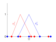
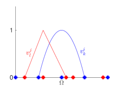
Thus for any i,j=0,,nformulae-sequence𝑖𝑗0𝑛i,j=0,\dotsc,n, we are able to compute the inner product vki,vljXsubscriptsuperscriptsubscript𝑣𝑘𝑖superscriptsubscript𝑣𝑙𝑗𝑋\langle v_{k}^{i},v_{l}^{j}\rangle_{X} for k=1,,Ni𝑘1subscript𝑁𝑖k=1,\dotsc,N_{i} and l=1,,Nj𝑙1subscript𝑁𝑗l=1,\dotsc,N_{j}, compare Figure 1. We discover, then, that the calculation of the matrix 𝒦𝒦\mathcal{K} as well as the determination of its eigenvectors can be done for any underlying finite element discretization. Thus, the eigenvectors {ϕi}i=1dsuperscriptsubscriptsubscriptitalic-ϕ𝑖𝑖1𝑑\{\phi_{i}\}_{i=1}^{d} of 𝒦𝒦\mathcal{K} are the right singular vectors of 𝒴𝒴\mathcal{Y} and contain the space independent time information. This fact will be used in the following to build up the reduced order model. We note that the calculation of the matrix 𝒦𝒦\mathcal{K} can be done for arbitrary finite element spaces, i.e. all kinds of adaptivity (hh-, p𝑝p- and r𝑟r-adaptivity) can be considered and we do not need a common reference mesh. The complexity of this methods lies in the computation of the inner products of the intersections of the finite elements, whereas in [49] the challenge lies in lifting the snapshots from different finite element spaces up to a common finite element space.
Refer to caption
Refer to caption
Figure 1: 1D finite element basis functions vljsuperscriptsubscript𝑣𝑙𝑗v_{l}^{j} and vkisuperscriptsubscript𝑣𝑘𝑖v_{k}^{i} on their corresponding grids. Left: both piecewise linear finite element ansatz functions. Right: piecewise linear and cubic finite element ansatz functions

Moreover, the calculation of the matrix 𝒦(n+1)×(n+1)𝒦superscript𝑛1𝑛1\mathcal{K}\in\mathbb{R}^{(n+1)\times(n+1)} (method of snapshots) is favorable, since we assume the temporal dimension n𝑛n to be far smaller than the spatial dimension(s). Due to the symmetry of 𝒦𝒦\mathcal{K} it suffices to compute the entries on and upon the diagonal of the matrix. The computations of the matrix entries of 𝒦𝒦\mathcal{K} can be done fully in parallel. Hence, if sufficiently good hardware is available, setting up the matrix 𝒦𝒦\mathcal{K} can be done very fast.

Example 3.2. We choose V=H1(Ω),H=L2(Ω)formulae-sequence𝑉superscript𝐻1Ω𝐻superscript𝐿2ΩV=H^{1}(\Omega),H=L^{2}(\Omega) and set X=H=L2(Ω)𝑋𝐻superscript𝐿2ΩX=H=L^{2}(\Omega). The triangulations of Ω¯¯Ω\bar{\Omega} for each time level j=0,,n𝑗0𝑛j=0,\dotsc,n are denoted by {𝒯j}j=0nsuperscriptsubscriptsubscript𝒯𝑗𝑗0𝑛\{\mathcal{T}_{j}\}_{j=0}^{n} and the finite element spaces are defined by

Vj=V(𝒯j)={vC0(Ω¯):v|Tr(T),T𝒯j}X,j=0,,n,formulae-sequencesubscript𝑉𝑗𝑉subscript𝒯𝑗conditional-set𝑣superscript𝐶0¯Ωformulae-sequenceevaluated-at𝑣𝑇subscript𝑟𝑇for-all𝑇subscript𝒯𝑗𝑋𝑗0𝑛V_{j}=V(\mathcal{T}_{j})=\{v\in C^{0}(\bar{\Omega}):v|_{T}\in\mathbb{P}_{r}(T),\forall T\in\mathcal{T}_{j}\}\subset X,\quad j=0,\dotsc,n,

where rsubscript𝑟\mathbb{P}_{r} denotes the space of polynomials of degree r𝑟r\in\mathbb{N}. The computation of the ij𝑖𝑗ij-th entry 𝒦ij=αiαjyi,yjL2(Ω)subscript𝒦𝑖𝑗subscript𝛼𝑖subscript𝛼𝑗subscriptsubscript𝑦𝑖subscript𝑦𝑗superscript𝐿2Ω\mathcal{K}_{ij}=\sqrt{\alpha_{i}}\sqrt{\alpha_{j}}\langle y_{i},y_{j}\rangle_{L^{2}(\Omega)} of the matrix 𝒦𝒦\mathcal{K} is calculated by

αiαjyi,yjL2(Ω)=αiαjΩyiyj𝑑x=αiαjk=1Nil=1Nj𝗒ki𝗒ljΩvkivlj𝑑x=αiαjk=1Nil=1Nj𝗒ki𝗒lj(T𝒯iT¯𝒯jTT¯vkivlj𝑑x).subscript𝛼𝑖subscript𝛼𝑗subscriptsubscript𝑦𝑖subscript𝑦𝑗superscript𝐿2Ωsubscript𝛼𝑖subscript𝛼𝑗subscriptΩsubscript𝑦𝑖subscript𝑦𝑗differential-d𝑥missing-subexpressionsubscript𝛼𝑖subscript𝛼𝑗superscriptsubscript𝑘1superscript𝑁𝑖superscriptsubscript𝑙1superscript𝑁𝑗superscriptsubscript𝗒𝑘𝑖superscriptsubscript𝗒𝑙𝑗subscriptΩsuperscriptsubscript𝑣𝑘𝑖superscriptsubscript𝑣𝑙𝑗differential-d𝑥missing-subexpressionsubscript𝛼𝑖subscript𝛼𝑗superscriptsubscript𝑘1superscript𝑁𝑖superscriptsubscript𝑙1superscript𝑁𝑗superscriptsubscript𝗒𝑘𝑖superscriptsubscript𝗒𝑙𝑗subscript𝑇subscript𝒯𝑖subscript¯𝑇subscript𝒯𝑗subscript𝑇¯𝑇superscriptsubscript𝑣𝑘𝑖superscriptsubscript𝑣𝑙𝑗differential-d𝑥\begin{array}[]{l c l}\sqrt{\alpha_{i}}\sqrt{\alpha_{j}}\langle y_{i},y_{j}\rangle_{L^{2}(\Omega)}&=&\sqrt{\alpha_{i}}\sqrt{\alpha_{j}}\displaystyle\int\limits_{\Omega}y_{i}y_{j}dx\\ &=&\sqrt{\alpha_{i}}\sqrt{\alpha_{j}}\displaystyle\sum_{k=1}^{N^{i}}\displaystyle\sum_{l=1}^{N^{j}}\mathsf{y}_{k}^{i}\mathsf{y}_{l}^{j}\displaystyle\int\limits_{\Omega}v_{k}^{i}v_{l}^{j}dx\\ &=&\sqrt{\alpha_{i}}\sqrt{\alpha_{j}}\displaystyle\sum_{k=1}^{N^{i}}\displaystyle\sum_{l=1}^{N^{j}}\mathsf{y}_{k}^{i}\mathsf{y}_{l}^{j}\left(\displaystyle\sum_{T\in\mathcal{T}_{i}}\;\displaystyle\sum_{\bar{T}\in\mathcal{T}_{j}}\;\displaystyle\int\limits_{T\cap\bar{T}}v_{k}^{i}v_{l}^{j}dx\right).\\ \end{array}

Computations become simpler when using nested grids. In this case, the intersection of two arbitrary n𝑛n-dimensional simplices coincides either with the smaller simplex, or is a common edge simplex, or has no overlap.

Example 3.2 reveals the challenge to deal with integrals of type

Pyiyj𝑑xsubscript𝑃subscript𝑦𝑖subscript𝑦𝑗differential-d𝑥\int_{P}y_{i}y_{j}dx (19)

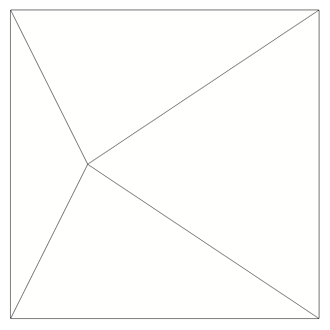
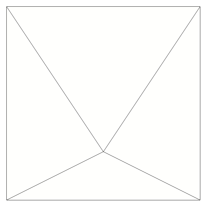
over cut finite elements (polyhedra) P=TT¯𝑃𝑇¯𝑇P=T\cap\bar{T} with T𝒯i𝑇subscript𝒯𝑖T\in\mathcal{T}_{i} and T¯𝒯j¯𝑇subscript𝒯𝑗\bar{T}\in\mathcal{T}_{j}, which involves the integration of functions defined on different (non-matching) meshes, compare Figure 2.
Refer to caption
Refer to caption
Refer to caption
Figure 2: Two finite element meshes (left, middle) and the overlapping mesh (right)

Our numerical realization is strongly based on [36], where a similar challenge is investigated in the context of multimesh methods. There, the major challenges are identified as (i) collision detection (find intersecting simplices), (ii) mesh intersection (detect intersection interface) and (iii) integration on complex polyhedra. In the numerical Example 6.3 we make use of built-in FEniCS [7, 32] tools to handle the issues (i) and (ii). For (iii) the integration over the cut elements, a subtriangulation can be an option. But as pointed out in [36] in the context of a three-dimensional example, a subtetrahedralization of an arbitrary polyhedron is challenging and additional vertices might have to be added. Therefore, an alternative approach is outlined which is based on a boundary representation of the integrals, compare [34, 37] for example. Exemplarily, in the case of a two-dimensional domain with piecewise linear finite element discretization, the integrals of type (19) can be computed as respectively weighted sum of the integrals

Px02𝑑x,Px12,Px0x1𝑑x,Px0𝑑x,Px1𝑑x,P1𝑑x,subscript𝑃superscriptsubscript𝑥02differential-d𝑥subscript𝑃superscriptsubscript𝑥12subscript𝑃subscript𝑥0subscript𝑥1differential-d𝑥subscript𝑃subscript𝑥0differential-d𝑥subscript𝑃subscript𝑥1differential-d𝑥subscript𝑃1differential-d𝑥\int_{P}x_{0}^{2}dx,\quad\int_{P}x_{1}^{2},\quad\int_{P}x_{0}x_{1}dx,\quad\int_{P}x_{0}dx,\quad\int_{P}x_{1}dx,\quad\int_{P}1dx, (20)

with x=(x0,x1)𝑥subscript𝑥0subscript𝑥1x=(x_{0},x_{1}) using Stoke’s formula

Pf(x)𝑑x=12+qi=1mbiaiEif(x)𝑑σi,subscript𝑃𝑓𝑥differential-d𝑥12𝑞superscriptsubscript𝑖1𝑚subscript𝑏𝑖normsubscript𝑎𝑖subscriptsubscript𝐸𝑖𝑓𝑥differential-dsubscript𝜎𝑖\int_{P}f(x)dx=\frac{1}{2+q}\sum_{i=1}^{m}\frac{b_{i}}{\|a_{i}\|}\int_{E_{i}}f(x)d\sigma_{i}, (21)

where {Ei}i=1msuperscriptsubscriptsubscript𝐸𝑖𝑖1𝑚\{E_{i}\}_{i=1}^{m} denote the edges of the polyhedron P2𝑃superscript2P\subset\mathbb{R}^{2}, aiTx=bisuperscriptsubscript𝑎𝑖𝑇𝑥subscript𝑏𝑖a_{i}^{T}x=b_{i} is the hyperplane in which Eisubscript𝐸𝑖E_{i} lies, and f𝑓f is a polynomial of degree q𝑞q. Note that the line integrals on the edges Eisubscript𝐸𝑖E_{i} can be computed using standard Gauss quadrature, for example.

4 POD reduced order modeling

4.1 POD reduced order modeling for arbitrary finite element discretizations

In this section, we stay in the infinite-dimensional setting of the POD method and set up the POD reduced order model utilizing snapshots with arbitrary finite element discretizations. This perspective allows us to determine the mode coefficients of the POD Galerkin ansatz for arbitrary underlying finite element discretizations. Suppose for given snapshots y0V0,,ynVnformulae-sequencesubscript𝑦0subscript𝑉0subscript𝑦𝑛subscript𝑉𝑛y_{0}\in V_{0},\dotsc,y_{n}\in V_{n} we have computed the matrix 𝒦𝒦\mathcal{K}, (16), with 𝒦ij=αiαjyi,yjXsubscript𝒦𝑖𝑗subscript𝛼𝑖subscript𝛼𝑗subscriptsubscript𝑦𝑖subscript𝑦𝑗𝑋\mathcal{K}_{ij}=\sqrt{\alpha_{i}}\sqrt{\alpha_{j}}\langle y_{i},y_{j}\rangle_{X}, for i,j=0,,nformulae-sequence𝑖𝑗0𝑛i,j=0,\dotsc,n as well as its \ell largest eigenvalues {λi}i=1superscriptsubscriptsubscript𝜆𝑖𝑖1\{\lambda_{i}\}_{i=1}^{\ell} and corresponding eigenvectors {ϕi}i=1n+1superscriptsubscriptsubscriptitalic-ϕ𝑖𝑖1superscript𝑛1\{\phi_{i}\}_{i=1}^{\ell}\subset\mathbb{R}^{n+1} of low rank \ell with n+1𝑛1\ell\leq n+1, according to the strategy presented in Section 3. The POD basis {ψi}i=1superscriptsubscriptsubscript𝜓𝑖𝑖1\{\psi_{i}\}_{i=1}^{\ell} is then given by (17), i.e

ψi=1λi𝒴ϕi for i=1,,.formulae-sequencesubscript𝜓𝑖1subscript𝜆𝑖𝒴subscriptitalic-ϕ𝑖 for 𝑖1\psi_{i}=\frac{1}{\sqrt{\lambda_{i}}}\mathcal{Y}\phi_{i}\quad\text{ for }i=1,\dotsc,\ell.

This POD basis is utilized in order to compute a reduced order model for (3). For this reason, we make the POD Galerkin ansatz

y(t)=i=1ηi(t)ψi=i=1ηi(t)1λi𝒴ϕifor all t[0,T],formulae-sequencesuperscript𝑦𝑡superscriptsubscript𝑖1subscript𝜂𝑖𝑡subscript𝜓𝑖superscriptsubscript𝑖1subscript𝜂𝑖𝑡1subscript𝜆𝑖𝒴subscriptitalic-ϕ𝑖for all 𝑡0𝑇y^{\ell}(t)=\displaystyle\sum\limits_{i=1}^{\ell}\eta_{i}(t)\psi_{i}=\displaystyle\sum\limits_{i=1}^{\ell}\eta_{i}(t)\frac{1}{\sqrt{\lambda_{i}}}\mathcal{Y}\phi_{i}\quad\text{for all }t\in[0,T], (22)

as an approximation for y(t)𝑦𝑡y(t), with the Fourier coefficients

ηi(t)=y(t),ψiX=y(t),1λi𝒴ϕiXsubscript𝜂𝑖𝑡subscriptsuperscript𝑦𝑡subscript𝜓𝑖𝑋subscriptsuperscript𝑦𝑡1subscript𝜆𝑖𝒴subscriptitalic-ϕ𝑖𝑋\eta_{i}(t)=\langle y^{\ell}(t),\psi_{i}\rangle_{X}=\langle y^{\ell}(t),\frac{1}{\sqrt{\lambda_{i}}}\mathcal{Y}\phi_{i}\rangle_{X}

for i=1,,𝑖1i=1,\dotsc,\ell. Inserting ysuperscript𝑦y^{\ell} into (3) and choosing V=span{ψ1,,ψ}Vsuperscript𝑉spansubscript𝜓1subscript𝜓𝑉V^{\ell}=\text{span}\{\psi_{1},\dotsc,\psi_{\ell}\}\subset V as the test space leads to the system

{ddty(t),ψH+a(y(t),ψ)+𝒩(y(t)),ψV,V=f(t),ψV,Vy(0),ψH=g,ψHcases𝑑𝑑𝑡subscriptsuperscript𝑦𝑡𝜓𝐻𝑎superscript𝑦𝑡𝜓subscript𝒩superscript𝑦𝑡𝜓superscript𝑉𝑉subscript𝑓𝑡𝜓superscript𝑉𝑉subscriptsuperscript𝑦0𝜓𝐻subscript𝑔𝜓𝐻\left\{\begin{array}[]{rcl}\displaystyle\frac{d}{dt}\langle y^{\ell}(t),\psi\rangle_{H}+a(y^{\ell}(t),\psi)+\langle\mathcal{N}(y^{\ell}(t)),\psi\rangle_{V^{\prime},V}&=&\langle f(t),\psi\rangle_{V^{\prime},V}\\ \langle y^{\ell}(0),\psi\rangle_{H}&=&\langle g,\psi\rangle_{H}\end{array}\right. (23)

for all ψV𝜓superscript𝑉\psi\in V^{\ell} and for almost all t(0,T]𝑡0𝑇t\in(0,T]. Utilizing the ansatz (22), we can write (23) as an \ell-dimensional ordinary differential equation system for the POD mode coefficients {ηi(t)}i=1superscriptsubscriptsubscript𝜂𝑖𝑡𝑖1\{\eta_{i}(t)\}_{i=1}^{\ell}\subset\mathbb{R}:

{j=1η˙j(t)ψi,ψjH+j=1ηj(t)𝒜ψj,ψiV,V+𝒩(y(t)),ψiV,V=f(t),ψiV,V for t(0,T],j=1ηj(0)ψi,ψjH=g,ψiH,casessuperscriptsubscript𝑗1subscript˙𝜂𝑗𝑡subscriptsubscript𝜓𝑖subscript𝜓𝑗𝐻superscriptsubscript𝑗1subscript𝜂𝑗𝑡subscript𝒜subscript𝜓𝑗subscript𝜓𝑖superscript𝑉𝑉subscript𝒩superscript𝑦𝑡subscript𝜓𝑖superscript𝑉𝑉subscript𝑓𝑡subscript𝜓𝑖superscript𝑉𝑉missing-subexpressionmissing-subexpression for 𝑡0𝑇superscriptsubscript𝑗1subscript𝜂𝑗0subscriptsubscript𝜓𝑖subscript𝜓𝑗𝐻subscript𝑔subscript𝜓𝑖𝐻\left\{\begin{array}[]{rcl}\displaystyle\sum_{j=1}^{\ell}{\dot{\eta}}_{j}(t)\langle\psi_{i},\psi_{j}\rangle_{H}+\displaystyle\sum_{j=1}^{\ell}\eta_{j}(t)\langle\mathcal{A}\psi_{j},\psi_{i}\rangle_{V^{\prime},V}+\langle\mathcal{N}(y^{\ell}(t)),\psi_{i}\rangle_{V^{\prime},V}&=&\langle f(t),\psi_{i}\rangle_{V^{\prime},V}\\ &&\hskip 28.45274pt\text{ for }t\in(0,T],\\ \displaystyle\sum_{j=1}^{\ell}\eta_{j}(0)\langle\psi_{i},\psi_{j}\rangle_{H}&=&\langle g,\psi_{i}\rangle_{H},\\ \end{array}\right. (24)

for i=1,,𝑖1i=1,\dotsc,\ell. Note that ψi,ψjH=δijsubscriptsubscript𝜓𝑖subscript𝜓𝑗𝐻subscript𝛿𝑖𝑗\langle\psi_{i},\psi_{j}\rangle_{H}=\delta_{ij} if we choose X=H𝑋𝐻X=H in the context of Section 3.

Since we want to construct a reduced order model which can be built and solved for arbitrary finite element discretizations, we rewrite system (24) utilizing the identity (17). Then, the system (24) can be written as

{j=1η˙j(t)1λi1λj𝒴ϕi,𝒴ϕjH+j=1ηj(t)1λi1λj𝒜𝒴ϕj,𝒴ϕiV,V+1λi𝒩(y(t)),𝒴ϕiV,V=1λif(t),𝒴ϕiV,V for t(0,T],j=1ηj(0)1λi1λj𝒴ϕi,𝒴ϕjH=1λig,𝒴ϕiH.casessuperscriptsubscript𝑗1subscript˙𝜂𝑗𝑡1subscript𝜆𝑖1subscript𝜆𝑗subscript𝒴subscriptitalic-ϕ𝑖𝒴subscriptitalic-ϕ𝑗𝐻superscriptsubscript𝑗1subscript𝜂𝑗𝑡1subscript𝜆𝑖1subscript𝜆𝑗subscript𝒜𝒴subscriptitalic-ϕ𝑗𝒴subscriptitalic-ϕ𝑖superscript𝑉𝑉missing-subexpressionmissing-subexpression1subscript𝜆𝑖subscript𝒩superscript𝑦𝑡𝒴subscriptitalic-ϕ𝑖superscript𝑉𝑉1subscript𝜆𝑖subscript𝑓𝑡𝒴subscriptitalic-ϕ𝑖superscript𝑉𝑉missing-subexpressionmissing-subexpression for 𝑡0𝑇superscriptsubscript𝑗1subscript𝜂𝑗01subscript𝜆𝑖1subscript𝜆𝑗subscript𝒴subscriptitalic-ϕ𝑖𝒴subscriptitalic-ϕ𝑗𝐻1subscript𝜆𝑖subscript𝑔𝒴subscriptitalic-ϕ𝑖𝐻\left\{\begin{array}[]{rcl}\displaystyle\sum_{j=1}^{\ell}{\dot{\eta}}_{j}(t)\displaystyle\frac{1}{\sqrt{\lambda_{i}}}\displaystyle\frac{1}{\sqrt{\lambda_{j}}}\langle\mathcal{Y}\phi_{i},\mathcal{Y}\phi_{j}\rangle_{H}+\displaystyle\sum_{j=1}^{\ell}\eta_{j}(t)\frac{1}{\sqrt{\lambda_{i}}}\frac{1}{\sqrt{\lambda_{j}}}\langle\mathcal{A}\mathcal{Y}\phi_{j},\mathcal{Y}\phi_{i}\rangle_{V^{\prime},V}&&\\ +\displaystyle\frac{1}{\sqrt{\lambda_{i}}}\langle\mathcal{N}(y^{\ell}(t)),\mathcal{Y}\phi_{i}\rangle_{V^{\prime},V}&=&\displaystyle\frac{1}{\sqrt{\lambda_{i}}}\langle f(t),\mathcal{Y}\phi_{i}\rangle_{V^{\prime},V}\\ &&\hskip 19.91684pt\text{ for }t\in(0,T],\\ \displaystyle\sum_{j=1}^{\ell}\eta_{j}(0)\frac{1}{\sqrt{\lambda_{i}}}\frac{1}{\sqrt{\lambda_{j}}}\langle\mathcal{Y}\phi_{i},\mathcal{Y}\phi_{j}\rangle_{H}&=&\displaystyle\frac{1}{\sqrt{\lambda_{i}}}\langle g,\mathcal{Y}\phi_{i}\rangle_{H}.\\ \end{array}\right. (25)

In order to write (25) in a compact matrix-vector form, let us introduce the diagonal matrix

D× with D=diag(1λ1,,1λ).𝐷superscript with 𝐷diag1subscript𝜆11subscript𝜆D\in\mathbb{R}^{\ell\times\ell}\text{ with }D=\text{diag}\left(\frac{1}{\sqrt{\lambda_{1}}},\dotsc,\frac{1}{\sqrt{\lambda_{\ell}}}\right).

From the first \ell eigenvectors {ϕi}i=1superscriptsubscriptsubscriptitalic-ϕ𝑖𝑖1\{\phi_{i}\}_{i=1}^{\ell} of 𝒦𝒦\mathcal{K} we build the matrix

Φ(n+1)× by Φ=[ϕ1||ϕ].Φsuperscript𝑛1 by Φdelimited-[]subscriptitalic-ϕ1subscriptitalic-ϕ\Phi\in\mathbb{R}^{(n+1)\times\ell}\text{ by }\Phi=[\phi_{1}\;|\;\dotsc\;|\;\phi_{\ell}].

Then, the system (25) can be written as the system

{DΦT𝒦ΦDη˙(t)+DΦT𝒴𝒜𝒴ΦDη(t)+DN(η(t))=DF(t) for t(0,T],DΦT𝒦ΦDη(0)=Dη¯0,cases𝐷superscriptΦ𝑇𝒦Φ𝐷˙𝜂𝑡𝐷superscriptΦ𝑇superscript𝒴𝒜𝒴Φ𝐷𝜂𝑡𝐷𝑁𝜂𝑡𝐷𝐹𝑡 for 𝑡0𝑇𝐷superscriptΦ𝑇𝒦Φ𝐷𝜂0𝐷subscript¯𝜂0missing-subexpression\left\{\begin{array}[]{rcll}D\Phi^{T}\mathcal{K}\Phi D\;{\dot{\eta}}(t)+D\Phi^{T}\mathcal{Y}^{\star}\mathcal{A}\mathcal{Y}\Phi D\;\eta(t)+DN(\eta(t))&=&DF(t)&\text{ for }t\in(0,T],\\ D\Phi^{T}\mathcal{K}\Phi D\;\eta(0)&=&D\bar{\eta}_{0},&\\ \end{array}\right. (26)

for the vector-valued mapping η(t)=(η1(t),,η(t))T:[0,T]:𝜂𝑡superscriptsubscript𝜂1𝑡subscript𝜂𝑡𝑇0𝑇superscript\eta(t)=(\eta_{1}(t),\dotsc,\eta_{\ell}(t))^{T}:[0,T]\to\mathbb{R}^{\ell}. Note that the right hand side F(t)𝐹𝑡F(t) and the initial condition η¯0subscript¯𝜂0\bar{\eta}_{0} are given by

(F(t))i=f(t),𝒴ϕiV,V=𝒴f(t),ϕin+1subscript𝐹𝑡𝑖subscript𝑓𝑡𝒴subscriptitalic-ϕ𝑖superscript𝑉𝑉subscriptsuperscript𝒴𝑓𝑡subscriptitalic-ϕ𝑖superscript𝑛1\left(F(t)\right)_{i}=\langle f(t),\mathcal{Y}\phi_{i}\rangle_{V^{\prime},V}=\langle\mathcal{Y}^{\star}f(t),\phi_{i}\rangle_{\mathbb{R}^{n+1}}

and

(η¯0)i=g,𝒴ϕiH=𝒴g,ϕin+1,subscriptsubscript¯𝜂0𝑖subscript𝑔𝒴subscriptitalic-ϕ𝑖𝐻subscriptsuperscript𝒴𝑔subscriptitalic-ϕ𝑖superscript𝑛1\left(\bar{\eta}_{0}\right)_{i}=\langle g,\mathcal{Y}\phi_{i}\rangle_{H}=\langle\mathcal{Y}^{\star}g,\phi_{i}\rangle_{\mathbb{R}^{n+1}},

for i=1,,𝑖1i=1,\dotsc,\ell, respectively. Their calculation can be done explicitly for any arbitrary finite element discretization. For a given function wV𝑤𝑉w\in V (for example w=f(t)𝑤𝑓𝑡w=f(t) or w=g𝑤𝑔w=g) with finite element discretization w=i=1Nw𝗐iφi𝑤superscriptsubscript𝑖1subscript𝑁𝑤subscript𝗐𝑖subscript𝜑𝑖w=\sum_{i=1}^{N_{w}}\mathsf{w}_{i}\varphi_{i}, nodal basis {φi}i=1NwVsuperscriptsubscriptsubscript𝜑𝑖𝑖1subscript𝑁𝑤𝑉\{\varphi_{i}\}_{i=1}^{N_{w}}\subset V and appropriate mode coefficients {𝗐i}i=1Nwsuperscriptsubscriptsubscript𝗐𝑖𝑖1subscript𝑁𝑤\{\mathsf{w}_{i}\}_{i=1}^{N_{w}} we can compute

(𝒴w)j=w,yjX=i=1Nw𝗐iφi,k=1Nj𝗒kjvkjX=i=1Nwk=1Nj𝗐i𝗒kjφi,vkjX, for j=0,,nformulae-sequencesubscriptsuperscript𝒴𝑤𝑗subscript𝑤subscript𝑦𝑗𝑋subscriptsuperscriptsubscript𝑖1subscript𝑁𝑤subscript𝗐𝑖subscript𝜑𝑖superscriptsubscript𝑘1subscript𝑁𝑗superscriptsubscript𝗒𝑘𝑗superscriptsubscript𝑣𝑘𝑗𝑋superscriptsubscript𝑖1subscript𝑁𝑤superscriptsubscript𝑘1subscript𝑁𝑗subscript𝗐𝑖superscriptsubscript𝗒𝑘𝑗subscriptsubscript𝜑𝑖superscriptsubscript𝑣𝑘𝑗𝑋 for 𝑗0𝑛\left(\mathcal{Y}^{\star}w\right)_{j}=\langle w,y_{j}\rangle_{X}=\langle\sum_{i=1}^{N_{w}}\mathsf{w}_{i}\varphi_{i},\sum_{k=1}^{N_{j}}\mathsf{y}_{k}^{j}v_{k}^{j}\rangle_{X}=\sum_{i=1}^{N_{w}}\sum_{k=1}^{N_{j}}\mathsf{w}_{i}\mathsf{y}_{k}^{j}\langle\varphi_{i},v_{k}^{j}\rangle_{X},\quad\text{ for }j=0,\dotsc,n

where yjVjsubscript𝑦𝑗subscript𝑉𝑗y_{j}\in V_{j} denotes the j𝑗j-th snapshot. Again, for any i=1,,Nw𝑖1subscript𝑁𝑤i=1,\dotsc,N_{w} and k=1,,Nj𝑘1subscript𝑁𝑗k=1,\dotsc,N_{j}, the computation of the inner product φi,vkjXsubscriptsubscript𝜑𝑖superscriptsubscript𝑣𝑘𝑗𝑋\langle\varphi_{i},v_{k}^{j}\rangle_{X} can be done explicitly.

Obviously, for linear evolution equations the POD reduced order model (26) can be set up and solved utilizing snapshots with arbitrary finite element discretizations. The computation of the nonlinear component N(η(t))𝑁𝜂𝑡N(\eta(t)) needs particular attention. In the following Section 4.2 we discuss the options to treat the nonlinearity.

Remark 4.1. Of course, the derivation of a POD surrogate model (26) for (3) as explained above, is also applicable for other classes of differential equations like elliptic PDEs, for example.

Time-discrete reduced order model

In order to solve the reduced order system (23) numerically, we apply the implicit Euler method for time discretization and use for simplicity the same temporal grid {tj}j=0nsuperscriptsubscriptsubscript𝑡𝑗𝑗0𝑛\{t_{j}\}_{j=0}^{n} (10) as for the snapshots. It is also possible to use a different time grid, cf. [30]. The time-discrete reduced order model reads

{yjyj1Δtj,ψH+a(yj,ψ)+𝒩(yj),ψV,V=1Δtjtj1tjfj,ψV,V for all ψV,y0,ψH=g,ψH,casessubscriptsuperscriptsubscript𝑦𝑗superscriptsubscript𝑦𝑗1Δsubscript𝑡𝑗𝜓𝐻𝑎superscriptsubscript𝑦𝑗𝜓subscript𝒩superscriptsubscript𝑦𝑗𝜓superscript𝑉𝑉1Δsubscript𝑡𝑗superscriptsubscriptsubscript𝑡𝑗1subscript𝑡𝑗subscriptsubscript𝑓𝑗𝜓superscript𝑉𝑉 for all 𝜓superscript𝑉subscriptsuperscriptsubscript𝑦0𝜓𝐻subscript𝑔𝜓𝐻missing-subexpression\left\{\begin{array}[]{rcll}\left\langle\displaystyle\frac{y_{j}^{\ell}-y_{j-1}^{\ell}}{\Delta t_{j}},\psi\right\rangle_{H}+a(y_{j}^{\ell},\psi)+\langle\mathcal{N}(y_{j}^{\ell}),\psi\rangle_{V^{\prime},V}&=&\displaystyle\frac{1}{\Delta t_{j}}\displaystyle\int_{t_{j-1}}^{t_{j}}\langle f_{j},\psi\rangle_{V^{\prime},V}&\text{ for all }\psi\in V^{\ell},\\ \langle y_{0}^{\ell},\psi\rangle_{H}&=&\langle g,\psi\rangle_{H},&\\ \end{array}\right. (27)

for j=1,,n𝑗1𝑛j=1,\dotsc,n or equivalently

{DΦT𝒦ΦD(ηjηj1Δtj)+DΦT𝒴𝒜𝒴ΦDηj+DN(ηj)=DFj for j=1,,n,DΦT𝒦ΦDη0=Dη¯0.cases𝐷superscriptΦ𝑇𝒦Φ𝐷superscript𝜂𝑗superscript𝜂𝑗1Δsubscript𝑡𝑗𝐷superscriptΦ𝑇superscript𝒴𝒜𝒴Φ𝐷superscript𝜂𝑗𝐷𝑁superscript𝜂𝑗𝐷subscript𝐹𝑗 for 𝑗1𝑛𝐷superscriptΦ𝑇𝒦Φ𝐷superscript𝜂0𝐷subscript¯𝜂0missing-subexpression\left\{\begin{array}[]{rcll}D\Phi^{T}\mathcal{K}\Phi D\;\left(\displaystyle\frac{\eta^{j}-\eta^{j-1}}{\Delta t_{j}}\right)+D\Phi^{T}\mathcal{Y}^{\star}\mathcal{A}\mathcal{Y}\Phi D\;\eta^{j}+DN(\eta^{j})&=&DF_{j}&\text{ for }j=1,\dotsc,n,\\ D\Phi^{T}\mathcal{K}\Phi D\;\eta^{0}&=&D\bar{\eta}_{0}.&\end{array}\right. (28)

4.2 Discussion of the nonlinear term 𝑫𝑵(𝜼(𝒕))𝑫𝑵𝜼𝒕\boldsymbol{DN(\eta(t))}

Let us now consider the computation of the nonlinear term DN(η(t))𝐷𝑁𝜂𝑡superscriptDN(\eta(t))\in\mathbb{R}^{\ell} of the POD-ROM (26). It holds true

(DN(η(t)))k=𝒩(y(t)),ψkV,V=𝒩(i=1ηi(t)ψi),ψkV,Vsubscript𝐷𝑁𝜂𝑡𝑘subscript𝒩superscript𝑦𝑡subscript𝜓𝑘superscript𝑉𝑉missing-subexpressionsubscript𝒩superscriptsubscript𝑖1subscript𝜂𝑖𝑡subscript𝜓𝑖subscript𝜓𝑘superscript𝑉𝑉\begin{array}[]{r c l}(DN(\eta(t)))_{k}&=&\langle\mathcal{N}(y^{\ell}(t)),\psi_{k}\rangle_{V^{\prime},V}\\[2.84544pt] &=&\langle\mathcal{N}(\sum_{i=1}^{\ell}\eta_{i}(t)\psi_{i}),\psi_{k}\rangle_{V^{\prime},V}\end{array}

for k=1,,𝑘1k=1,\cdots,\ell. It is well-known that the evaluation of nonlinearities in the reduced order model context in computationally expensive. To make this clear, let us assume, we are given a uniform finite element discretization with N𝑁N degrees of freedom. Then, in the fully discrete setting, the nonlinear term has the form

ΨTW𝒩(Ψη(t)),superscriptΨ𝑇𝑊𝒩Ψ𝜂𝑡\Psi^{T}W\mathcal{N}(\Psi\eta(t)),

where Ψ=[ψ1||ψ]N×Ψdelimited-[]subscript𝜓1subscript𝜓superscript𝑁\Psi=\left[\psi_{1}\;|\;\cdots\;|\;\psi_{\ell}\right]\in\mathbb{R}^{N\times\ell} is the matrix in which the POD modes are stored columnwise and WN×N𝑊superscript𝑁𝑁W\in\mathbb{R}^{N\times N} is a weighting matrix related to the utilized inner product. Hence, the treatment of the nonlinearity requires the expansion of y(t)=Ψη(t)Nsuperscript𝑦𝑡Ψ𝜂𝑡superscript𝑁y^{\ell}(t)=\Psi\eta(t)\in\mathbb{R}^{N} in the full space, then the nonlinearity can be evaluated and finally the result is projected back to the POD space. Obviously, this means that the reduced order model is not fully independent of the high order dimension and efficient simulation cannot be guaranteed. Therefore, it is convenient to seek for hyper reduction, i.e. for a treatment of the nonlinearity where the model evaluation cost is related to the low dimension \ell. A possible remedy which is commonly used, is given discrete by empirical interpolation methods, for which we refer to [15] for DEIM and to [16] for Q-DEIM. Another option is given by [6] which investigates nonlinear model reduction via dynamic mode decomposition. Furthermore, in [52] nonlinear model reduction is realized by replacing the nonlinear term by its interpolation into the finite element space. The treatment of the nonlinearity is done in [8] by the missing point estimation method and in [38] by best the points interpolation method.
All these methods have in common, that a common reference mesh is needed. Since we want to circumvent the interpolation of the snapshots onto a common grid and we want to set up the reduced order model for arbitrary finite element discretizations, we have to go a different way.

One option is to utilize EIM [10] which is a hyper reduction technique formulated in a continuous setting. Alternatively, we can linearize and project the nonlinearity onto the POD space. For this approach, let us consider the linear reduced order system given by:

{ddty(t),ψH+a(y(t),ψ)+𝒩(y¯(t)),ψV,V=f(t),vV,V,y(0),ψH=g,vH,cases𝑑𝑑𝑡subscriptsuperscript𝑦𝑡𝜓𝐻𝑎superscript𝑦𝑡𝜓subscript𝒩¯𝑦𝑡𝜓superscript𝑉𝑉subscript𝑓𝑡𝑣superscript𝑉𝑉subscriptsuperscript𝑦0𝜓𝐻subscript𝑔𝑣𝐻\left\{\begin{array}[]{rcl}\frac{d}{dt}\langle y^{\ell}(t),\psi\rangle_{H}+a(y^{\ell}(t),\psi)+\langle\mathcal{N}(\bar{y}(t)),\psi\rangle_{V^{\prime},V}&=&\langle f(t),v\rangle_{V^{\prime},V},\\ \langle y^{\ell}(0),\psi\rangle_{H}&=&\langle g,v\rangle_{H},\\ \end{array}\right. (29)

For a given state y¯(t)V¯𝑦𝑡𝑉\bar{y}(t)\in V, this linear evolution problem (29) can be set up and solved explicitly without spatial interpolation. In the numerical examples in Section 6, we take the finite element solution as given state in each time step, i.e. y¯(tj)=yj¯𝑦subscript𝑡𝑗subscript𝑦𝑗\bar{y}(t_{j})=y_{j}.
Furthermore, the linearization of the reduced order model (23) can be considered:

{ddty(t),ψH+a(y(t),ψ)+𝒩(y¯(t))+𝒩y(y¯(t))(yy¯)(t),ψV,V=f(t),vV,V,y(0),ψH=g,vH,cases𝑑𝑑𝑡subscriptsuperscript𝑦𝑡𝜓𝐻𝑎superscript𝑦𝑡𝜓subscript𝒩¯𝑦𝑡subscript𝒩𝑦¯𝑦𝑡superscript𝑦¯𝑦𝑡𝜓superscript𝑉𝑉subscript𝑓𝑡𝑣superscript𝑉𝑉subscriptsuperscript𝑦0𝜓𝐻subscript𝑔𝑣𝐻\left\{\begin{array}[]{rcl}\frac{d}{dt}\langle y^{\ell}(t),\psi\rangle_{H}+a(y^{\ell}(t),\psi)+\langle\mathcal{N}(\bar{y}(t))+\mathcal{N}_{y}(\bar{y}(t))(y^{\ell}-\bar{y})(t),\psi\rangle_{V^{\prime},V}&=&\langle f(t),v\rangle_{V^{\prime},V},\\ \langle y^{\ell}(0),\psi\rangle_{H}&=&\langle g,v\rangle_{H},\\ \end{array}\right. (30)

where 𝒩ysubscript𝒩𝑦\mathcal{N}_{y} denotes the Fréchet derivative. This linearized problem is of interest in the context of optimal control, where it occurs in each iteration level within the SQP method, see [27], for example. Choosing the finite element solution as given state in each time instance leads to:

𝒩(yj),ψiV,V=1λik=0nαk(ϕi)k𝒩(yj),ykV,V𝒩y(yj)y(tj),ψiV,V=𝒩y(yj)(k=1ηk(tj)ψk),ψiV,V=k=1ηk(tj)1λk1λip=0nr=0nαpαr(ϕk)p(ϕi)r𝒩y(yj)yp,yrV,V𝒩y(yj)yj,ψiV,V=1λik=0nαk(ϕi)k𝒩y(yj)yj,ykV,Vsubscript𝒩subscript𝑦𝑗subscript𝜓𝑖superscript𝑉𝑉1subscript𝜆𝑖superscriptsubscript𝑘0𝑛subscript𝛼𝑘subscriptsubscriptϕ𝑖𝑘subscript𝒩subscript𝑦𝑗subscript𝑦𝑘superscript𝑉𝑉subscriptsubscript𝒩𝑦subscript𝑦𝑗superscript𝑦subscript𝑡𝑗subscript𝜓𝑖superscript𝑉𝑉subscriptsubscript𝒩𝑦subscript𝑦𝑗superscriptsubscript𝑘1subscript𝜂𝑘subscript𝑡𝑗subscript𝜓𝑘subscript𝜓𝑖superscript𝑉𝑉missing-subexpressionsuperscriptsubscript𝑘1subscript𝜂𝑘subscript𝑡𝑗1subscript𝜆𝑘1subscript𝜆𝑖superscriptsubscript𝑝0𝑛superscriptsubscript𝑟0𝑛subscript𝛼𝑝subscript𝛼𝑟subscriptsubscriptϕ𝑘𝑝subscriptsubscriptϕ𝑖𝑟subscriptsubscript𝒩𝑦subscript𝑦𝑗subscript𝑦𝑝subscript𝑦𝑟superscript𝑉𝑉subscriptsubscript𝒩𝑦subscript𝑦𝑗subscript𝑦𝑗subscript𝜓𝑖superscript𝑉𝑉1subscript𝜆𝑖superscriptsubscript𝑘0𝑛subscript𝛼𝑘subscriptsubscriptϕ𝑖𝑘subscriptsubscript𝒩𝑦subscript𝑦𝑗subscript𝑦𝑗subscript𝑦𝑘superscript𝑉𝑉\begin{array}[]{l c l}\langle\mathcal{N}(y_{j}),\psi_{i}\rangle_{V^{\prime},V}&=&\frac{1}{\sqrt{\lambda_{i}}}\sum_{k=0}^{n}\sqrt{\alpha_{k}}(\upphi_{i})_{k}\langle\mathcal{N}(y_{j}),y_{k}\rangle_{V^{\prime},V}\\[5.69046pt] \langle\mathcal{N}_{y}(y_{j})y^{\ell}(t_{j}),\psi_{i}\rangle_{V^{\prime},V}&=&\langle\mathcal{N}_{y}(y_{j})(\sum_{k=1}^{\ell}\eta_{k}(t_{j})\psi_{k}),\psi_{i}\rangle_{V^{\prime},V}\\[5.69046pt] &=&\sum_{k=1}^{\ell}\eta_{k}(t_{j})\frac{1}{\sqrt{\lambda_{k}}}\frac{1}{\sqrt{\lambda_{i}}}\sum_{p=0}^{n}\sum_{r=0}^{n}\sqrt{\alpha_{p}}\sqrt{\alpha_{r}}(\upphi_{k})_{p}(\upphi_{i})_{r}\langle\mathcal{N}_{y}(y_{j})y_{p},y_{r}\rangle_{V^{\prime},V}\\[5.69046pt] \langle\mathcal{N}_{y}(y_{j})y_{j},\psi_{i}\rangle_{V^{\prime},V}&=&\frac{1}{\sqrt{\lambda_{i}}}\sum_{k=0}^{n}\sqrt{\alpha_{k}}(\upphi_{i})_{k}\langle\mathcal{N}_{y}(y_{j})y_{j},y_{k}\rangle_{V^{\prime},V}\end{array}

Finally, we approximate the nonlinearity DN(ηj)𝐷𝑁superscript𝜂𝑗DN(\eta^{j}) in (28) by

(DN(ηj))k𝒩(yj)+𝒩y(yj)(y(tj)yj),ψkV,Vsubscript𝐷𝑁superscript𝜂𝑗𝑘subscript𝒩subscript𝑦𝑗subscript𝒩𝑦subscript𝑦𝑗superscript𝑦subscript𝑡𝑗subscript𝑦𝑗subscript𝜓𝑘superscript𝑉𝑉(DN(\eta^{j}))_{k}\approx\langle\mathcal{N}(y_{j})+\mathcal{N}_{y}(y_{j})(y^{\ell}(t_{j})-y_{j}),\psi_{k}\rangle_{V^{\prime},V}

which can be written as

DN(ηj)DΦT𝖭j+DΦT𝙽yjΦDηjDΦT𝖭yj𝐷𝑁superscript𝜂𝑗𝐷superscriptΦ𝑇superscript𝖭𝑗𝐷superscriptΦ𝑇superscriptsubscript𝙽𝑦𝑗Φ𝐷superscript𝜂𝑗𝐷superscriptΦ𝑇superscriptsubscript𝖭𝑦𝑗DN(\eta^{j})\approx D\Phi^{T}\mathsf{N}^{j}+D\Phi^{T}\mathtt{N}_{y}^{j}\Phi D\eta^{j}-D\Phi^{T}\mathsf{N}_{y}^{j}

where

𝖭j=(𝒩(yj),α0y0V,V𝒩(yj),αnynV,V)n+1,𝖭yj=(𝒩y(yj)yj,α0y0V,V𝒩y(yj)yj,αnynV,V)n+1formulae-sequencesuperscript𝖭𝑗matrixsubscript𝒩subscript𝑦𝑗subscript𝛼0subscript𝑦0superscript𝑉𝑉subscript𝒩subscript𝑦𝑗subscript𝛼𝑛subscript𝑦𝑛superscript𝑉𝑉superscript𝑛1superscriptsubscript𝖭𝑦𝑗matrixsubscriptsubscript𝒩𝑦subscript𝑦𝑗subscript𝑦𝑗subscript𝛼0subscript𝑦0superscript𝑉𝑉subscriptsubscript𝒩𝑦subscript𝑦𝑗subscript𝑦𝑗subscript𝛼𝑛subscript𝑦𝑛superscript𝑉𝑉superscript𝑛1\mathsf{N}^{j}=\begin{pmatrix}\langle\mathcal{N}(y_{j}),\sqrt{\alpha_{0}}y_{0}\rangle_{V^{\prime},V}\\ \vdots\\ \langle\mathcal{N}(y_{j}),\sqrt{\alpha_{n}}y_{n}\rangle_{V^{\prime},V}\\ \end{pmatrix}\in\mathbb{R}^{n+1},\mathsf{N}_{y}^{j}=\begin{pmatrix}\langle\mathcal{N}_{y}(y_{j})y_{j},\sqrt{\alpha_{0}}y_{0}\rangle_{V^{\prime},V}\\ \vdots\\ \langle\mathcal{N}_{y}(y_{j})y_{j},\sqrt{\alpha_{n}}y_{n}\rangle_{V^{\prime},V}\\ \end{pmatrix}\in\mathbb{R}^{n+1}

and
𝙽yj=(𝒩y(yj)α0y0,α0y0V,V𝒩y(yj)αnyn,α0y0V,V𝒩y(yj)α0y0,αnynV,V𝒩y(yj)αnyn,αnynV,V)(n+1)×(n+1)superscriptsubscript𝙽𝑦𝑗matrixsubscriptsubscript𝒩𝑦subscript𝑦𝑗subscript𝛼0subscript𝑦0subscript𝛼0subscript𝑦0superscript𝑉𝑉subscriptsubscript𝒩𝑦subscript𝑦𝑗subscript𝛼𝑛subscript𝑦𝑛subscript𝛼0subscript𝑦0superscript𝑉𝑉missing-subexpressionsubscriptsubscript𝒩𝑦subscript𝑦𝑗subscript𝛼0subscript𝑦0subscript𝛼𝑛subscript𝑦𝑛superscript𝑉𝑉subscriptsubscript𝒩𝑦subscript𝑦𝑗subscript𝛼𝑛subscript𝑦𝑛subscript𝛼𝑛subscript𝑦𝑛superscript𝑉𝑉superscript𝑛1𝑛1\mathtt{N}_{y}^{j}=\begin{pmatrix}\langle\mathcal{N}_{y}(y_{j})\sqrt{\alpha_{0}}y_{0},\sqrt{\alpha_{0}}y_{0}\rangle_{V^{\prime},V}&\ldots&\langle\mathcal{N}_{y}(y_{j})\sqrt{\alpha_{n}}y_{n},\sqrt{\alpha_{0}}y_{0}\rangle_{V^{\prime},V}\\ \vdots&&\vdots\\ \langle\mathcal{N}_{y}(y_{j})\sqrt{\alpha_{0}}y_{0},\sqrt{\alpha_{n}}y_{n}\rangle_{V^{\prime},V}&\ldots&\langle\mathcal{N}_{y}(y_{j})\sqrt{\alpha_{n}}y_{n},\sqrt{\alpha_{n}}y_{n}\rangle_{V^{\prime},V}\\ \end{pmatrix}\in\mathbb{R}^{(n+1)\times(n+1)}

For weakly nonlinear systems this approximation may be sufficient, depending on the problem and its goal. A great advantage of linearizing the semilinear partial differential equation is that only linear equations need to be solved which leads to a further speedup. However, if a more precise approximation is desired or necessary, we can think of approximations including higher order terms, like quadratic approximation, see e.g. [12] and [45], or Taylor expansions, see e.g. [40], [41] and [19]. Nevertheless, the efficiency of higher order approximations is limited due to growing memory and computational costs.

4.3 Expressing the POD solution in the full spatial domain

Having determined the solution η(t)𝜂𝑡\eta(t) to (26), we can set up the reduced solution y(t)superscript𝑦𝑡y^{\ell}(t) in a continuous framework:

y(t)=i=1ηi(t)(1λij=0nαj(ϕi)jyj).superscript𝑦𝑡superscriptsubscript𝑖1subscript𝜂𝑖𝑡1subscript𝜆𝑖superscriptsubscript𝑗0𝑛subscript𝛼𝑗subscriptsubscriptϕ𝑖𝑗subscript𝑦𝑗y^{\ell}(t)=\sum_{i=1}^{\ell}\eta_{i}(t)\left(\frac{1}{\sqrt{\lambda_{i}}}\sum_{j=0}^{n}\sqrt{\alpha_{j}}(\upphi_{i})_{j}y_{j}\right). (31)

Now, let us turn to the fully discrete formulation of (31). For a time-discrete setting, we introduce for simplicity the same temporal grid {tj}j=0nsuperscriptsubscriptsubscript𝑡𝑗𝑗0𝑛\{t_{j}\}_{j=0}^{n} as for the snapshots. Let us recall the spatial discretization of the snapshots (13) utilizing arbitrary finite elements

yj=k=1Nj𝗒kjvkj for j=0,,n.formulae-sequencesubscript𝑦𝑗superscriptsubscript𝑘1subscript𝑁𝑗superscriptsubscript𝗒𝑘𝑗superscriptsubscript𝑣𝑘𝑗 for 𝑗0𝑛y_{j}=\displaystyle\sum_{k=1}^{N_{j}}\mathsf{y}_{k}^{j}v_{k}^{j}\quad\text{ for }j=0,\dotsc,n.

Let {Qrj}r=1Mjsuperscriptsubscriptsuperscriptsubscript𝑄𝑟𝑗𝑟1subscript𝑀𝑗\{Q_{r}^{j}\}_{r=1}^{M_{j}} denote an arbitrary set of grid points for the reduced system at time level tjsubscript𝑡𝑗t_{j}. The fully discrete POD solution can be computed by evaluation:

y(tj,Qrj)=i=1ηi(tj)(1λis=0nαs(ϕi)s(k=1Ns𝗒ksvks(Qrj)))superscript𝑦subscript𝑡𝑗superscriptsubscript𝑄𝑟𝑗superscriptsubscript𝑖1subscript𝜂𝑖subscript𝑡𝑗1subscript𝜆𝑖superscriptsubscript𝑠0𝑛subscript𝛼𝑠subscriptsubscriptϕ𝑖𝑠superscriptsubscript𝑘1subscript𝑁𝑠superscriptsubscript𝗒𝑘𝑠superscriptsubscript𝑣𝑘𝑠superscriptsubscript𝑄𝑟𝑗y^{\ell}(t_{j},Q_{r}^{j})=\sum_{i=1}^{\ell}\eta_{i}(t_{j})\left(\frac{1}{\sqrt{\lambda_{i}}}\sum_{s=0}^{n}\sqrt{\alpha_{s}}(\upphi_{i})_{s}(\sum_{k=1}^{N_{s}}\mathsf{y}_{k}^{s}v_{k}^{s}(Q_{r}^{j}))\right) (32)

for j=0,,n𝑗0𝑛j=0,\dotsc,n and r=1,,Mj𝑟1subscript𝑀𝑗r=1,\dotsc,M_{j}. This allows us to use any grid for expressing the POD solution in the full spatial domain. For example, we can use the same node points at time level j𝑗j for the POD simulation as we have used for the snapshots, i.e. for j=0,,n𝑗0𝑛j=0,\dotsc,n it holds Mj=Njsubscript𝑀𝑗subscript𝑁𝑗M_{j}=N_{j} and Qrj=Pkjsuperscriptsubscript𝑄𝑟𝑗superscriptsubscript𝑃𝑘𝑗Q_{r}^{j}=P_{k}^{j} for all r,k=1,,Njformulae-sequence𝑟𝑘1subscript𝑁𝑗r,k=1,\dotsc,N_{j}. Another option can be to choose

{Qrj}r=1Mj=j=0nk=1Nj{Pkj},superscriptsubscriptsuperscriptsubscript𝑄𝑟𝑗𝑟1subscript𝑀𝑗superscriptsubscript𝑗0𝑛superscriptsubscript𝑘1subscript𝑁𝑗superscriptsubscript𝑃𝑘𝑗\{Q_{r}^{j}\}_{r=1}^{M_{j}}=\displaystyle\bigcup_{j=0}^{n}\bigcup_{k=1}^{N_{j}}\{P_{k}^{j}\},

i.e. the common finest grid. Obviously, a special and probably the easiest case concerning the implementation is to choose snapshots which are expressed with respect to the same finite element basis functions and utilize the common finest grid for the simulation of the reduced order system, which is proposed by [49]. After expressing the adaptively sampled snapshots with respect to a common finite element space, the subsequent steps coincide with the common approach of taking snapshots which are generated without adaptivity. Then, expression (32) simplifies to

y(tj,Prj)=i=1ηi(tj)(1λis=0nαs(ϕi)s𝗒s).superscript𝑦subscript𝑡𝑗superscriptsubscript𝑃𝑟𝑗superscriptsubscript𝑖1subscript𝜂𝑖subscript𝑡𝑗1subscript𝜆𝑖superscriptsubscript𝑠0𝑛subscript𝛼𝑠subscriptsubscriptϕ𝑖𝑠superscript𝗒𝑠y^{\ell}(t_{j},P_{r}^{j})=\sum_{i=1}^{\ell}\eta_{i}(t_{j})\left(\frac{1}{\sqrt{\lambda_{i}}}\sum_{s=0}^{n}\sqrt{\alpha_{s}}(\upphi_{i})_{s}\mathsf{y}^{s}\right). (33)

5 Error analysis for the reduced order model

For the validation of the approximation quality of the POD reduced order model, we are interested in analyzing the error between the POD solution and the true solution. Our aim is to estimate the expression

j=0nαjy(tj)yjH2superscriptsubscript𝑗0𝑛subscript𝛼𝑗superscriptsubscriptnorm𝑦subscript𝑡𝑗superscriptsubscript𝑦𝑗𝐻2\sum_{j=0}^{n}\alpha_{j}\|y(t_{j})-y_{j}^{\ell}\|_{H}^{2}

where {y(tj)}j=0nVsuperscriptsubscript𝑦subscript𝑡𝑗𝑗0𝑛𝑉\{y(t_{j})\}_{j=0}^{n}\subset V denotes the true solution for (3) at time instances {tj}j=0nsuperscriptsubscriptsubscript𝑡𝑗𝑗0𝑛\{t_{j}\}_{j=0}^{n} and {yj}j=0nsuperscriptsubscriptsuperscriptsubscript𝑦𝑗𝑗0𝑛\{y_{j}^{\ell}\}_{j=0}^{n} is the solution to the time-discrete reduced order model (27), i.e.

yj=i=1ηijψi,superscriptsubscript𝑦𝑗superscriptsubscript𝑖1superscriptsubscript𝜂𝑖𝑗subscript𝜓𝑖y_{j}^{\ell}=\sum_{i=1}^{\ell}\eta_{i}^{j}\psi_{i}, (34)

with the POD basis {ψi}i=1superscriptsubscriptsubscript𝜓𝑖𝑖1\{\psi_{i}\}_{i=1}^{\ell} computed from the snapshots {yj}j=0nsuperscriptsubscriptsubscript𝑦𝑗𝑗0𝑛\{y_{j}\}_{j=0}^{n} from arbitrary finite element spaces, i.e. yjVjsubscript𝑦𝑗subscript𝑉𝑗y_{j}\in V_{j} for j=0,,n𝑗0𝑛j=0,\dotsc,n, as explained in Section 3. The weights {αj}j=0nsuperscriptsubscriptsubscript𝛼𝑗𝑗0𝑛\{\alpha_{j}\}_{j=0}^{n} are trapezoidal time weights, see (15). We choose X=V𝑋𝑉X=V in the context of Section 3. Let us introduce the orthogonal projection 𝒫:VV:superscript𝒫𝑉superscript𝑉\mathcal{P}^{\ell}:V\to V^{\ell} by

𝒫v=i=1v,ψiVψi for all vV.formulae-sequencesuperscript𝒫𝑣superscriptsubscript𝑖1subscript𝑣subscript𝜓𝑖𝑉subscript𝜓𝑖 for all 𝑣𝑉\mathcal{P}^{\ell}v=\displaystyle\sum_{i=1}^{\ell}\langle v,\psi_{i}\rangle_{V}\psi_{i}\quad\text{ for all }v\in V.

It holds true 𝒫(V)=1subscriptnormsuperscript𝒫𝑉1\|\mathcal{P}^{\ell}\|_{\mathcal{L}(V)}=1, where (V)𝑉\mathcal{L}(V) is the space of linear bounded operators from V𝑉V to V𝑉V. The subsequent calculations follow closely the proofs of [30, Thm. 4.7] [51, Thm. 3.2.5] and [29, Th. 7]. In our situation, we compute the POD basis corresponding to the fully discrete snapshots {yj}j=0nsuperscriptsubscriptsubscript𝑦𝑗𝑗0𝑛\{y_{j}\}_{j=0}^{n} utilizing adaptive finite element spaces, whereas in [30], [51] and [29], the POD basis is computed from snapshots corresponding to the solution trajectory at the given time instances. For this reason, in the following estimation an additional term corresponding to the error for the spatial discretization will appear.

We make use of the decomposition

y(tj)yj=y(tj)yj+yj𝒫yj+𝒫yj𝒫y(tj)+𝒫y(tj)yj=ηj+ϱj+ζj+ϑj𝑦subscript𝑡𝑗superscriptsubscript𝑦𝑗𝑦subscript𝑡𝑗subscript𝑦𝑗subscript𝑦𝑗superscript𝒫subscript𝑦𝑗superscript𝒫subscript𝑦𝑗superscript𝒫𝑦subscript𝑡𝑗superscript𝒫𝑦subscript𝑡𝑗superscriptsubscript𝑦𝑗subscript𝜂𝑗subscriptitalic-ϱ𝑗subscript𝜁𝑗subscriptitalic-ϑ𝑗y(t_{j})-y_{j}^{\ell}=y(t_{j})-y_{j}+y_{j}-\mathcal{P}^{\ell}y_{j}+\mathcal{P}^{\ell}y_{j}-\mathcal{P}^{\ell}y(t_{j})+\mathcal{P}^{\ell}y(t_{j})-y_{j}^{\ell}=\eta_{j}+\varrho_{j}+\zeta_{j}+\vartheta_{j} (35)

for j=0,,n𝑗0𝑛j=0,\dotsc,n, where ηj:=y(tj)yj,ϱj:=yj𝒫yj,ζj=𝒫yj𝒫y(tj)formulae-sequenceassignsubscript𝜂𝑗𝑦subscript𝑡𝑗subscript𝑦𝑗formulae-sequenceassignsubscriptitalic-ϱ𝑗subscript𝑦𝑗superscript𝒫subscript𝑦𝑗subscript𝜁𝑗superscript𝒫subscript𝑦𝑗superscript𝒫𝑦subscript𝑡𝑗\eta_{j}:=y(t_{j})-y_{j},\varrho_{j}:=y_{j}-\mathcal{P}^{\ell}y_{j},\zeta_{j}=\mathcal{P}^{\ell}y_{j}-\mathcal{P}^{\ell}y(t_{j}) and ϑj:=𝒫y(tj)yjassignsubscriptitalic-ϑ𝑗superscript𝒫𝑦subscript𝑡𝑗superscriptsubscript𝑦𝑗\vartheta_{j}:=\mathcal{P}^{\ell}y(t_{j})-y_{j}^{\ell}. The term ηjsubscript𝜂𝑗\eta_{j} is the discretization error. We utilize the decomposition

ηj=y(tj)yj=y(tj)y¯j+y¯jyj=Etj+Ehjsubscript𝜂𝑗𝑦subscript𝑡𝑗subscript𝑦𝑗𝑦subscript𝑡𝑗subscript¯𝑦𝑗subscript¯𝑦𝑗subscript𝑦𝑗superscriptsubscript𝐸𝑡𝑗superscriptsubscript𝐸𝑗\eta_{j}=y(t_{j})-y_{j}=y(t_{j})-\bar{y}_{j}+\bar{y}_{j}-y_{j}=E_{t}^{j}+E_{h}^{j}

where y¯jsubscript¯𝑦𝑗\bar{y}_{j} denotes the solution to the time-discrete problem (11). By Etj:=y(tj)y¯jassignsuperscriptsubscript𝐸𝑡𝑗𝑦subscript𝑡𝑗subscript¯𝑦𝑗E_{t}^{j}:=y(t_{j})-\bar{y}_{j} we denote the global time discretization error and Ehj:=y¯jyjassignsuperscriptsubscript𝐸𝑗subscript¯𝑦𝑗subscript𝑦𝑗E_{h}^{j}:=\bar{y}_{j}-y_{j} is the global spatial discretization error. It is

EhjHmaxj=0,,nEhjH=:εh\|E_{h}^{j}\|_{H}\leq\max_{j=0,\dotsc,n}\|E_{h}^{j}\|_{H}=:\varepsilon_{h}

and

EtjHmaxj=0,,nEtjH=:εt.\|E_{t}^{j}\|_{H}\leq\max_{j=0,\dotsc,n}\|E_{t}^{j}\|_{H}=:\varepsilon_{t}.

Since we use the implicit Euler method for time integration, it is εt=𝒪(Δt)subscript𝜀𝑡𝒪Δ𝑡\varepsilon_{t}=\mathcal{O}(\Delta t) with Δt:=maxj=0,,nΔtjassignΔ𝑡subscript𝑗0𝑛Δsubscript𝑡𝑗\Delta t:=\max_{j=0,\dotsc,n}\Delta t_{j}. Therefore, we can estimate

j=0nαjy(tj)yjH2j=0nαjEtj+EhjH22j=0nαj((Δt)2+εh2)2T((Δt)2+εh2).superscriptsubscript𝑗0𝑛subscript𝛼𝑗superscriptsubscriptnorm𝑦subscript𝑡𝑗subscript𝑦𝑗𝐻2superscriptsubscript𝑗0𝑛subscript𝛼𝑗superscriptsubscriptnormsuperscriptsubscript𝐸𝑡𝑗superscriptsubscript𝐸𝑗𝐻22superscriptsubscript𝑗0𝑛subscript𝛼𝑗superscriptΔ𝑡2superscriptsubscript𝜀22𝑇superscriptΔ𝑡2superscriptsubscript𝜀2\sum_{j=0}^{n}\alpha_{j}\|y(t_{j})-y_{j}\|_{H}^{2}\leq\sum_{j=0}^{n}\alpha_{j}\|E_{t}^{j}+E_{h}^{j}\|_{H}^{2}\leq 2\sum_{j=0}^{n}\alpha_{j}((\Delta t)^{2}+\varepsilon_{h}^{2})\leq 2T((\Delta t)^{2}+\varepsilon_{h}^{2}). (36)

Moreover, we have

j=0nαjζjH2=j=0nαj𝒫yj𝒫y(tj)H2𝒫(H)2j=0nαjηjH2.superscriptsubscript𝑗0𝑛subscript𝛼𝑗superscriptsubscriptnormsubscript𝜁𝑗𝐻2superscriptsubscript𝑗0𝑛subscript𝛼𝑗superscriptsubscriptnormsuperscript𝒫subscript𝑦𝑗superscript𝒫𝑦subscript𝑡𝑗𝐻2superscriptsubscriptnormsuperscript𝒫𝐻2superscriptsubscript𝑗0𝑛subscript𝛼𝑗superscriptsubscriptnormsubscript𝜂𝑗𝐻2\sum_{j=0}^{n}\alpha_{j}\|\zeta_{j}\|_{H}^{2}=\sum_{j=0}^{n}\alpha_{j}\|\mathcal{P}^{\ell}y_{j}-\mathcal{P}^{\ell}y(t_{j})\|_{H}^{2}\leq\|\mathcal{P}^{\ell}\|_{\mathcal{L}(H)}^{2}\sum_{j=0}^{n}\alpha_{j}\|\eta_{j}\|_{H}^{2}. (37)

The term ϱjsubscriptitalic-ϱ𝑗\varrho_{j} is the projection error of the snapshot yjsubscript𝑦𝑗y_{j} projected onto the POD space Vsuperscript𝑉V^{\ell}. Using (1), the weighted sum of all projection errors is given by the sum of the neglected eigenvalues (18), i.e.

j=0nαjϱjH2=j=0nαjyji=1yj,ψiVψiH2cvj=0nαjyji=1yj,ψiVψiV2cvi=+1dλi.superscriptsubscript𝑗0𝑛subscript𝛼𝑗superscriptsubscriptnormsubscriptitalic-ϱ𝑗𝐻2superscriptsubscript𝑗0𝑛subscript𝛼𝑗superscriptsubscriptnormsubscript𝑦𝑗superscriptsubscript𝑖1subscriptsubscript𝑦𝑗subscript𝜓𝑖𝑉subscript𝜓𝑖𝐻2subscript𝑐𝑣superscriptsubscript𝑗0𝑛subscript𝛼𝑗superscriptsubscriptnormsubscript𝑦𝑗superscriptsubscript𝑖1subscriptsubscript𝑦𝑗subscript𝜓𝑖𝑉subscript𝜓𝑖𝑉2subscript𝑐𝑣superscriptsubscript𝑖1𝑑subscript𝜆𝑖\sum_{j=0}^{n}\alpha_{j}\|\varrho_{j}\|_{H}^{2}=\sum_{j=0}^{n}\alpha_{j}\|y_{j}-\sum_{i=1}^{\ell}\langle y_{j},\psi_{i}\rangle_{V}\psi_{i}\|_{H}^{2}\leq c_{v}\sum_{j=0}^{n}\alpha_{j}\|y_{j}-\sum_{i=1}^{\ell}\langle y_{j},\psi_{i}\rangle_{V}\psi_{i}\|_{V}^{2}\leq c_{v}\sum_{i=\ell+1}^{d}\lambda_{i}. (38)

It remains to estimate the term ϑjsubscriptitalic-ϑ𝑗\vartheta_{j} which is the error between the projection of the true solution y(tj)𝑦subscript𝑡𝑗y(t_{j}) at time instance tjsubscript𝑡𝑗t_{j} onto the POD space Vsuperscript𝑉V^{\ell} and the time-discrete ROM solution yjsuperscriptsubscript𝑦𝑗y_{j}^{\ell} to (34). With the use of the notation ¯ϑj=(ϑjϑj1)/Δtj¯subscriptitalic-ϑ𝑗subscriptitalic-ϑ𝑗subscriptitalic-ϑ𝑗1Δsubscript𝑡𝑗\bar{\partial}\vartheta_{j}=(\vartheta_{j}-\vartheta_{j-1})/\Delta t_{j} for j=1,,n𝑗1𝑛j=1,\dotsc,n, we get

¯ϑj,ψH=𝒫(y(tj)y(tj1)Δtj)yjyj1Δtj,ψH=𝒫(y(tj)y(tj1)Δtj)+𝒩(yj)fj,ψH+a(yj,ψ)=𝒫(y(tj)y(tj1)Δtj)y(tj)y(tj1)Δtj+𝒩(yj)𝒩(y(tj)),ψH+a(yjy(tj),ψ)=zj+𝒩(yj)𝒩(y(tj)),ψH+a(yjy(tj),ψ)subscript¯subscriptitalic-ϑ𝑗𝜓𝐻subscriptsuperscript𝒫𝑦subscript𝑡𝑗𝑦subscript𝑡𝑗1Δsubscript𝑡𝑗superscriptsubscript𝑦𝑗superscriptsubscript𝑦𝑗1Δsubscript𝑡𝑗𝜓𝐻missing-subexpressionsubscriptsuperscript𝒫𝑦subscript𝑡𝑗𝑦subscript𝑡𝑗1Δsubscript𝑡𝑗𝒩superscriptsubscript𝑦𝑗subscript𝑓𝑗𝜓𝐻𝑎superscriptsubscript𝑦𝑗𝜓missing-subexpressionsubscriptsuperscript𝒫𝑦subscript𝑡𝑗𝑦subscript𝑡𝑗1Δsubscript𝑡𝑗𝑦subscript𝑡𝑗𝑦subscript𝑡𝑗1Δsubscript𝑡𝑗𝒩superscriptsubscript𝑦𝑗𝒩𝑦subscript𝑡𝑗𝜓𝐻𝑎superscriptsubscript𝑦𝑗𝑦subscript𝑡𝑗𝜓missing-subexpressionsubscriptsubscript𝑧𝑗𝒩superscriptsubscript𝑦𝑗𝒩𝑦subscript𝑡𝑗𝜓𝐻𝑎superscriptsubscript𝑦𝑗𝑦subscript𝑡𝑗𝜓\left.\begin{array}[]{rcl}\langle\bar{\partial}\vartheta_{j},\psi\rangle_{H}&=&\langle\mathcal{P}^{\ell}\left(\displaystyle\frac{y(t_{j})-y(t_{j-1})}{\Delta t_{j}}\right)-\displaystyle\frac{y_{j}^{\ell}-y_{j-1}^{\ell}}{\Delta t_{j}},\psi\rangle_{H}\\ &=&\langle\mathcal{P}^{\ell}\left(\displaystyle\frac{y(t_{j})-y(t_{j-1})}{\Delta t_{j}}\right)+\mathcal{N}(y_{j}^{\ell})-f_{j},\psi\rangle_{H}+a(y_{j}^{\ell},\psi)\\ &=&\langle\mathcal{P}^{\ell}\left(\displaystyle\frac{y(t_{j})-y(t_{j-1})}{\Delta t_{j}}\right)-\displaystyle\frac{y(t_{j})-y(t_{j-1})}{\Delta t_{j}}+\mathcal{N}(y_{j}^{\ell})-\mathcal{N}(y(t_{j})),\psi\rangle_{H}+a(y_{j}^{\ell}-y(t_{j}),\psi)\\ &=&\langle z_{j}+\mathcal{N}(y_{j}^{\ell})-\mathcal{N}(y(t_{j})),\psi\rangle_{H}+a(y_{j}^{\ell}-y(t_{j}),\psi)\end{array}\right.

for ψV𝜓superscript𝑉\psi\in V^{\ell} with zj:=𝒫(y(tj)y(tj1)Δtj)y(tj)y(tj1)Δtjassignsubscript𝑧𝑗𝒫𝑦subscript𝑡𝑗𝑦subscript𝑡𝑗1Δsubscript𝑡𝑗𝑦subscript𝑡𝑗𝑦subscript𝑡𝑗1Δsubscript𝑡𝑗z_{j}:=\mathcal{P}\left(\displaystyle\frac{y(t_{j})-y(t_{j-1})}{\Delta t_{j}}\right)-\displaystyle\frac{y(t_{j})-y(t_{j-1})}{\Delta t_{j}}. With the choice ψ=ϑj𝜓subscriptitalic-ϑ𝑗\psi=\vartheta_{j} and the use of the identity

2uv,u=u2v2+uv22𝑢𝑣𝑢superscriptnorm𝑢2superscriptnorm𝑣2superscriptnorm𝑢𝑣22\langle u-v,u\rangle=\|u\|^{2}-\|v\|^{2}+\|u-v\|^{2}

we obtain

ϑjH2ϑj1H2+2Δtj(βyjy(tj)H+zjH+𝒩(yj)𝒩(y(tj))H)ϑjH,superscriptsubscriptnormsubscriptitalic-ϑ𝑗𝐻2superscriptsubscriptnormsubscriptitalic-ϑ𝑗1𝐻22Δsubscript𝑡𝑗𝛽subscriptnormsuperscriptsubscript𝑦𝑗𝑦subscript𝑡𝑗𝐻subscriptnormsubscript𝑧𝑗𝐻subscriptnorm𝒩superscriptsubscript𝑦𝑗𝒩𝑦subscript𝑡𝑗𝐻subscriptnormsubscriptitalic-ϑ𝑗𝐻\|\vartheta_{j}\|_{H}^{2}\leq\|\vartheta_{j-1}\|_{H}^{2}+2\Delta t_{j}\left(\beta\|y_{j}^{\ell}-y(t_{j})\|_{H}+\|z_{j}\|_{H}+\|\mathcal{N}(y_{j}^{\ell})-\mathcal{N}(y(t_{j}))\|_{H}\right)\|\vartheta_{j}\|_{H},

where we have utilized (2). We assume that 𝒩𝒩\mathcal{N} is Lipschitz continuous, i.e. there exists L>0𝐿0L>0 such that

𝒩(yj)𝒩(y(tj))HLyjy(tj)H for j=1,,n.formulae-sequencesubscriptnorm𝒩superscriptsubscript𝑦𝑗𝒩𝑦subscript𝑡𝑗𝐻𝐿subscriptnormsuperscriptsubscript𝑦𝑗𝑦subscript𝑡𝑗𝐻 for 𝑗1𝑛\|\mathcal{N}(y_{j}^{\ell})-\mathcal{N}(y(t_{j}))\|_{H}\leq L\|y_{j}^{\ell}-y(t_{j})\|_{H}\quad\text{ for }j=1,\dotsc,n.

Applying Young’s inequality we find

ϑjH2ϑj1H2+Δtj(c1ϱjH2+c2ϑjH2+zjH2+c1ηjH2+c1ζjH2)superscriptsubscriptnormsubscriptitalic-ϑ𝑗𝐻2superscriptsubscriptnormsubscriptitalic-ϑ𝑗1𝐻2Δsubscript𝑡𝑗subscript𝑐1superscriptsubscriptnormsubscriptitalic-ϱ𝑗𝐻2subscript𝑐2superscriptsubscriptnormsubscriptitalic-ϑ𝑗𝐻2superscriptsubscriptnormsubscript𝑧𝑗𝐻2subscript𝑐1superscriptsubscriptnormsubscript𝜂𝑗𝐻2subscript𝑐1superscriptsubscriptnormsubscript𝜁𝑗𝐻2\|\vartheta_{j}\|_{H}^{2}\leq\|\vartheta_{j-1}\|_{H}^{2}+\Delta t_{j}(c_{1}\|\varrho_{j}\|_{H}^{2}+c_{2}\|\vartheta_{j}\|_{H}^{2}+\|z_{j}\|_{H}^{2}+c_{1}\|\eta_{j}\|_{H}^{2}+c_{1}\|\zeta_{j}\|_{H}^{2})

with the constants c1:=β+Lassignsubscript𝑐1𝛽𝐿c_{1}:=\beta+L and c2:=5(β+L)+1assignsubscript𝑐25𝛽𝐿1c_{2}:=5(\beta+L)+1. Under the assumption that ΔtΔ𝑡\Delta t is sufficiently small, we conclude

ϑjH2e2c2jΔt(ϑ1H2+k=1jΔtk(zkH2+c1ϱkH2+c1ηkH2+c1ζkH2)).superscriptsubscriptnormsubscriptitalic-ϑ𝑗𝐻2superscript𝑒2subscript𝑐2𝑗Δ𝑡superscriptsubscriptnormsubscriptitalic-ϑ1𝐻2superscriptsubscript𝑘1𝑗Δsubscript𝑡𝑘superscriptsubscriptnormsubscript𝑧𝑘𝐻2subscript𝑐1superscriptsubscriptnormsubscriptitalic-ϱ𝑘𝐻2subscript𝑐1superscriptsubscriptnormsubscript𝜂𝑘𝐻2subscript𝑐1superscriptsubscriptnormsubscript𝜁𝑘𝐻2\|\vartheta_{j}\|_{H}^{2}\leq e^{2c_{2}j\Delta t}\left(\|\vartheta_{1}\|_{H}^{2}+\sum_{k=1}^{j}\Delta t_{k}(\|z_{k}\|_{H}^{2}+c_{1}\|\varrho_{k}\|_{H}^{2}+c_{1}\|\eta_{k}\|_{H}^{2}+c_{1}\|\zeta_{k}\|_{H}^{2})\right). (39)

For more details on this, we refer to [30] and [51]. We choose the initial condition for (27) such that ϑ0=𝒫y(t0)y0=𝒫gy0=0subscriptitalic-ϑ0superscript𝒫𝑦subscript𝑡0superscriptsubscript𝑦0superscript𝒫𝑔superscriptsubscript𝑦00\vartheta_{0}=\mathcal{P}^{\ell}y(t_{0})-y_{0}^{\ell}=\mathcal{P}^{\ell}g-y_{0}^{\ell}=0.

Next, we estimate the term involving zksubscript𝑧𝑘z_{k}. It holds true

zkH2=𝒫(y(tk)y(tk1)Δtk)y(tk)y(tk1)ΔtkH2=𝒫(y(tk)y(tk1)Δtk)𝒫y˙(tk)+𝒫y˙(tk)y˙(tk)+y˙(tk)y(tk)y(tk1)ΔtkH22𝒫(H)2y(tk)y(tk1)Δtky˙(tk)H2+2𝒫y˙(tk)y˙(tk)H2+2y˙(tk)y(tk)y(tk1)ΔtkH2c3wkH2+2𝒫y˙(tk)y˙(tk)H2superscriptsubscriptnormsubscript𝑧𝑘𝐻2superscriptsubscriptnormsuperscript𝒫𝑦subscript𝑡𝑘𝑦subscript𝑡𝑘1Δsubscript𝑡𝑘𝑦subscript𝑡𝑘𝑦subscript𝑡𝑘1Δsubscript𝑡𝑘𝐻2missing-subexpressionsuperscriptsubscriptnormsuperscript𝒫𝑦subscript𝑡𝑘𝑦subscript𝑡𝑘1Δsubscript𝑡𝑘superscript𝒫˙𝑦subscript𝑡𝑘superscript𝒫˙𝑦subscript𝑡𝑘˙𝑦subscript𝑡𝑘˙𝑦subscript𝑡𝑘𝑦subscript𝑡𝑘𝑦subscript𝑡𝑘1Δsubscript𝑡𝑘𝐻2missing-subexpression2superscriptsubscriptnormsuperscript𝒫𝐻2superscriptsubscriptnorm𝑦subscript𝑡𝑘𝑦subscript𝑡𝑘1Δsubscript𝑡𝑘˙𝑦subscript𝑡𝑘𝐻22superscriptsubscriptnormsuperscript𝒫˙𝑦subscript𝑡𝑘˙𝑦subscript𝑡𝑘𝐻22superscriptsubscriptnorm˙𝑦subscript𝑡𝑘𝑦subscript𝑡𝑘𝑦subscript𝑡𝑘1Δsubscript𝑡𝑘𝐻2missing-subexpressionsubscript𝑐3superscriptsubscriptnormsubscript𝑤𝑘𝐻22superscriptsubscriptnormsuperscript𝒫˙𝑦subscript𝑡𝑘˙𝑦subscript𝑡𝑘𝐻2\left.\begin{array}[]{rcl}\|z_{k}\|_{H}^{2}&=&\|\mathcal{P}^{\ell}\left(\displaystyle\frac{y(t_{k})-y(t_{k-1})}{\Delta t_{k}}\right)-\displaystyle\frac{y(t_{k})-y(t_{k-1})}{\Delta t_{k}}\|_{H}^{2}\\ &=&\|\mathcal{P}^{\ell}\left(\displaystyle\frac{y(t_{k})-y(t_{k-1})}{\Delta t_{k}}\right)-\mathcal{P}^{\ell}\dot{y}(t_{k})+\mathcal{P}^{\ell}\dot{y}(t_{k})-\dot{y}(t_{k})+\dot{y}(t_{k})-\displaystyle\frac{y(t_{k})-y(t_{k-1})}{\Delta t_{k}}\|_{H}^{2}\\ &\leq&2\|\mathcal{P}^{\ell}\|_{\mathcal{L}(H)}^{2}\|\displaystyle\frac{y(t_{k})-y(t_{k-1})}{\Delta t_{k}}-\dot{y}(t_{k})\|_{H}^{2}+2\|\mathcal{P}^{\ell}\dot{y}(t_{k})-\dot{y}(t_{k})\|_{H}^{2}+2\|\dot{y}(t_{k})-\displaystyle\frac{y(t_{k})-y(t_{k-1})}{\Delta t_{k}}\|_{H}^{2}\\ &\leq&c_{3}\|w_{k}\|_{H}^{2}+2\|\mathcal{P}^{\ell}\dot{y}(t_{k})-\dot{y}(t_{k})\|_{H}^{2}\end{array}\right.

with c3=2+2𝒫(H)2subscript𝑐322superscriptsubscriptnormsuperscript𝒫𝐻2c_{3}=2+2\|\mathcal{P}^{\ell}\|_{\mathcal{L}(H)}^{2} and wk:=y˙(tk)y(tk)y(tk1)Δtkassignsubscript𝑤𝑘˙𝑦subscript𝑡𝑘𝑦subscript𝑡𝑘𝑦subscript𝑡𝑘1Δsubscript𝑡𝑘w_{k}:=\dot{y}(t_{k})-\displaystyle\frac{y(t_{k})-y(t_{k-1})}{\Delta t_{k}}, which can be estimated as

k=1jΔtkwkH2(Δt)23y¨L2(0,tj,H)2.superscriptsubscript𝑘1𝑗Δsubscript𝑡𝑘superscriptsubscriptnormsubscript𝑤𝑘𝐻2superscriptΔ𝑡23superscriptsubscriptnorm¨𝑦superscript𝐿20subscript𝑡𝑗𝐻2\sum_{k=1}^{j}\Delta t_{k}\|w_{k}\|_{H}^{2}\leq\frac{(\Delta t)^{2}}{3}\|\ddot{y}\|_{L^{2}(0,t_{j},H)}^{2}.

For more details on this, we refer to [30] and [51].

Finally, we can summarize the estimation for the term involving ϑjsubscriptitalic-ϑ𝑗\vartheta_{j} by

ϑjH2c4(k=1nαk(𝒫y˙(tk)y˙(tk)H2+ϱkH2+ηkH2+ζkH2)+(Δt)2y¨L2(0,T,H)2)superscriptsubscriptnormsubscriptitalic-ϑ𝑗𝐻2subscript𝑐4superscriptsubscript𝑘1𝑛subscript𝛼𝑘superscriptsubscriptnormsuperscript𝒫˙𝑦subscript𝑡𝑘˙𝑦subscript𝑡𝑘𝐻2superscriptsubscriptnormsubscriptitalic-ϱ𝑘𝐻2superscriptsubscriptnormsubscript𝜂𝑘𝐻2superscriptsubscriptnormsubscript𝜁𝑘𝐻2superscriptΔ𝑡2superscriptsubscriptnorm¨𝑦superscript𝐿20𝑇𝐻2\|\vartheta_{j}\|_{H}^{2}\leq c_{4}\left(\displaystyle\sum_{k=1}^{n}\alpha_{k}(\|\mathcal{P}^{\ell}\dot{y}(t_{k})-\dot{y}(t_{k})\|_{H}^{2}+\|\varrho_{k}\|_{H}^{2}+\|\eta_{k}\|_{H}^{2}+\|\zeta_{k}\|_{H}^{2})+(\Delta t)^{2}\|\ddot{y}\|_{L^{2}(0,T,H)}^{2}\right)

with c4:=e2c2Tmax{c33,4,2c1}assignsubscript𝑐4superscript𝑒2subscript𝑐2𝑇subscript𝑐3342subscript𝑐1c_{4}:=e^{2c_{2}T}\max\{\frac{c_{3}}{3},4,2c_{1}\} and thus it is

j=0nαjϑjH2c4T(j=0nαj𝒫y˙(tj)y˙(tj)H2+(Δt)2y¨L2(0,T,H)2+i=+1dλi+2T(1+𝒫(H)2)((Δt)2+εh2))\left.\begin{array}[]{rcl}\displaystyle\sum_{j=0}^{n}\alpha_{j}\|\vartheta_{j}\|_{H}^{2}&\leq&c_{4}T(\displaystyle\sum_{j=0}^{n}\alpha_{j}\|\mathcal{P}^{\ell}\dot{y}(t_{j})-\dot{y}(t_{j})\|_{H}^{2}+(\Delta t)^{2}\|\ddot{y}\|_{L^{2}(0,T,H)}^{2}+\sum_{i=\ell+1}^{d}\lambda_{i}\\ &&+2T(1+\|\mathcal{P}^{\ell}\|_{\mathcal{L}(H)}^{2})((\Delta t)^{2}+\varepsilon_{h}^{2}))\\ \end{array}\right. (40)

Theorem 5.1. Let {y(tj)}j=0nsuperscriptsubscript𝑦subscript𝑡𝑗𝑗0𝑛\{y(t_{j})\}_{j=0}^{n} denote the solution to problem (3) at the time grid {tj}j=0nsuperscriptsubscriptsubscript𝑡𝑗𝑗0𝑛\{t_{j}\}_{j=0}^{n} and yjsuperscriptsubscript𝑦𝑗y_{j}^{\ell} is the solution to (27). Let the nonlinear operator 𝒩𝒩\mathcal{N} be Lipschitz continuous with Lipschitz constant L𝐿L and the maximal time step Δt:=maxj=0,,nΔtjassignΔ𝑡subscript𝑗0𝑛Δsubscript𝑡𝑗\Delta t:=\max_{j=0,\dotsc,n}\Delta t_{j} be sufficiently small. Furthermore, we assume y¨(t)¨𝑦𝑡\ddot{y}(t) to be bounded on [0,T]0𝑇[0,T]. We choose the initial condition for (27) such that 𝒫g=y0superscript𝒫𝑔superscriptsubscript𝑦0\mathcal{P}^{\ell}g=y_{0}^{\ell} is fulfilled. Then, there exists a constant C=C(T,cv,P(H)2,β,L,y¨L2(0,T,H)2)>0𝐶𝐶𝑇subscript𝑐𝑣superscriptsubscriptnormsuperscript𝑃𝐻2𝛽𝐿superscriptsubscriptnorm¨𝑦superscript𝐿20𝑇𝐻20C=C(T,c_{v},\|P^{\ell}\|_{\mathcal{L}(H)}^{2},\beta,L,\|\ddot{y}\|_{L^{2}(0,T,H)}^{2})>0 such that

j=0nαjy(tj)yjH2C((Δt)2+εh2+i=+1dλi+j=0nαj𝒫y˙(tj)y˙(tj)H2),superscriptsubscript𝑗0𝑛subscript𝛼𝑗superscriptsubscriptnorm𝑦subscript𝑡𝑗superscriptsubscript𝑦𝑗𝐻2𝐶superscriptΔ𝑡2superscriptsubscript𝜀2superscriptsubscript𝑖1𝑑subscript𝜆𝑖superscriptsubscript𝑗0𝑛subscript𝛼𝑗superscriptsubscriptnormsuperscript𝒫˙𝑦subscript𝑡𝑗˙𝑦subscript𝑡𝑗𝐻2\displaystyle\sum_{j=0}^{n}\alpha_{j}\|y(t_{j})-y_{j}^{\ell}\|_{H}^{2}\leq C\left((\Delta t)^{2}+\varepsilon_{h}^{2}+\displaystyle\sum_{i=\ell+1}^{d}\lambda_{i}+\displaystyle\sum_{j=0}^{n}\alpha_{j}\|\mathcal{P}^{\ell}\dot{y}(t_{j})-\dot{y}(t_{j})\|_{H}^{2}\right), (41)

where cv,βsubscript𝑐𝑣𝛽c_{v},\beta are from (1),(2), the quantity εh:=maxj=0,,nyjy¯jHassignsubscript𝜀subscript𝑗0𝑛subscriptnormsubscript𝑦𝑗subscript¯𝑦𝑗𝐻\varepsilon_{h}:=\max_{j=0,\dotsc,n}\|y_{j}-\bar{y}_{j}\|_{H} refers to the global spatial discretization error and y¯jsubscript¯𝑦𝑗\bar{y}_{j} is the solution to (11) at time instance tjsubscript𝑡𝑗t_{j}.

Proof. Utilizing the decomposition (35) we infer

j=0nαjy(tj)yjH22j=0nαj(ηjH2+ϱjH2+ζjH2+ϑjH2).superscriptsubscript𝑗0𝑛subscript𝛼𝑗superscriptsubscriptnorm𝑦subscript𝑡𝑗superscriptsubscript𝑦𝑗𝐻22superscriptsubscript𝑗0𝑛subscript𝛼𝑗superscriptsubscriptnormsubscript𝜂𝑗𝐻2superscriptsubscriptnormsubscriptitalic-ϱ𝑗𝐻2superscriptsubscriptnormsubscript𝜁𝑗𝐻2superscriptsubscriptnormsubscriptitalic-ϑ𝑗𝐻2\displaystyle\sum_{j=0}^{n}\alpha_{j}\|y(t_{j})-y_{j}^{\ell}\|_{H}^{2}\leq 2\displaystyle\sum_{j=0}^{n}\alpha_{j}(\|\eta_{j}\|_{H}^{2}+\|\varrho_{j}\|_{H}^{2}+\|\zeta_{j}\|_{H}^{2}+\|\vartheta_{j}\|_{H}^{2}).

Together with (36), (37), (38) and (40) this leads to the claim.                                \square

Remark 5.2. i) The last term in (41) can be avoided by adding time derivatives to the snapshot set (more specifically, finite difference approximations of time derivatives), cf. [29]. In the recent work [47], a new error bound is proved which avoids the last term in (41) and does not need to include time derivative data in the POD snapshot set.
ii) If we choose V=H1(Ω)𝑉superscript𝐻1ΩV=H^{1}(\Omega) and H=L2(Ω)𝐻superscript𝐿2ΩH=L^{2}(\Omega) and utilize a static piecewise linear finite element discretization with hh being the diameter of the triangles, then εh=𝒪(h2)subscript𝜀𝒪superscript2\varepsilon_{h}=\mathcal{O}(h^{2}). In the case of adaptively refined spatial grids εhsubscript𝜀\varepsilon_{h} can be estimated by the prescribed error tolerance, if e.g. residual based a-posteriori error estimation is applied.

6 Numerical Realization and Examples

For all numerical examples, we choose Ω2Ωsuperscript2\Omega\subset\mathbb{R}^{2} as open and bounded domain and utilize conformal, piecewise linear and continuous finite elements for spatial discretization.
In Example 6.1 and 6.2, we utilize an hh-adaptive concept, which controls the spatial discretization error in the energy-norm. As error indicator for the adaptive strategy with respect to space we utilize at each time step the jump across the edges, which reflects the main contribution of the classical residual-based error estimation for elliptic problems, see e.g. (2.18)-(2.19) in [4]. The error indicator is given by

ηE=hE[yj]EνEL2(E) for all E,formulae-sequencesubscript𝜂𝐸subscript𝐸superscriptsubscriptnormsubscriptdelimited-[]subscript𝑦𝑗𝐸subscript𝜈𝐸𝐿2𝐸 for all 𝐸\eta_{E}=\sqrt{h_{E}}\|\left[\nabla y_{j}\right]_{E}\cdot\nu_{E}\|_{L}^{2}(E)\quad\text{ for all }E\in\mathcal{E}, (42)

where hEsubscript𝐸h_{E} is the length of the edge, [.]E\left[\;.\;\right]_{E} denotes the jump of the function across the edge E𝐸E, νEsubscript𝜈𝐸\nu_{E} is the outward normal derivative on the edge E𝐸E and \mathcal{E} denotes the collection of all (interior) edges in the current triangulation. As refinement rule we use the bisection by newest vertex based on [13].

In Example 6.1 and 6.2, we utilize structured, hierarchical and nested grids. These numerical test cases illustrate our approach to set up and solve a POD reduced order model utilizing snapshots with adaptive spatial discretization, which is explained in Section 3 and 4 in the specific case in which a nested mesh structure is at hand. Thus, the computations benefit from the fact that the intersection of two triangles coincides either with the smaller triangle, or is a common edge, or has no overlap. We compare our approach to the use of a uniform mesh, where the mesh size coincides with the fineness of the smallest triangle in the adaptive mesh. The aim of this comparison is to investigate numerically how the inclusion of spatial adaptivity for the snapshot discretization affects the accuracy of the POD reduced order solution compared to using a uniform mesh where no spatial adaptation is performed. Furthermore, we compare our approach to the use of a finest mesh following [49] concerning numerical efficiency and accuracy. For this, the practical numerical concept works as follows. In a full dimensional simulation, hh-adaptive snapshots are generated at the time instances {tj}j=0nsuperscriptsubscriptsubscript𝑡𝑗𝑗0𝑛\{t_{j}\}_{j=0}^{n}. At the same time we carry along a reference grid with the simulation, which coincides with the computational grid at initial time and which is only refined in the same manner as the computational grid. In this way, the reference grid becomes the finest mesh (i.e. the overlay of all computational grids) at the end of the snapshot generation. Then, the snapshots are expressed with respect to the finite element basis functions corresponding to the finest mesh and the usual POD procedure is carried out, choosing X=L2(Ω)𝑋superscript𝐿2ΩX=L^{2}(\Omega) as Hilbert space.
In Example 6.3 we realize the numerical computation of the correlation matrix 𝒦𝒦\mathcal{K} (16) as described in Section 3.2 for non-nested meshes. In this case, the overlap of two meshes leads to cut finite elements, which are convex polygons of more than three node points. Thus, numerical computations become more involved.
All coding is done in C++ and we utilize FEniCS [7, 32] for the solution of the differential equations and ALBERTA [46] for dealing with hierarchical meshes. We run the numerical tests on a compute server with 24 CPU kernels and 512 GB RAM.

Example 6.1: Linear heat equation. We consider the Example 2.3 (4) of a heat equation with homogeneous Dirichlet boundary condition and set c0𝑐0c\equiv 0 such that the equation becomes linear. The spatial domain is chosen as Ω=[0,1]×[0,1]2Ω0101superscript2\Omega=[0,1]\times[0,1]\subset\mathbb{R}^{2}, the time interval is [0,T]=[0,1.57]0𝑇01.57[0,T]=[0,1.57]. We construct an example in such a way that we know the analytical solution. It is given by

y(t,x)=r(t,x)(s1(t,x)s2(t,x))𝑦𝑡𝑥𝑟𝑡𝑥subscript𝑠1𝑡𝑥subscript𝑠2𝑡𝑥y(t,x)=r(t,x)\cdot\left(s_{1}(t,x)-s_{2}(t,x)\right)

with

r(t,x)=50000x0(1x0)(0.5+cos(t)(x00.5)sin(t)(x10.5))41t+1(1(0.5+cos(t)(x00.5)sin(t)(x10.5)))4)1+1000(cos(t)(x00.5)sin(t)(x10.5))2,r(t,x)=\frac{50000\cdot x_{0}\cdot(1-x_{0})\cdot(0.5+\cos(t)\cdot(x_{0}-0.5)-\sin(t)\cdot(x_{1}-0.5))^{4}\cdot\frac{1}{t+1}\cdot(1-(0.5+\cos(t)\cdot(x_{0}-0.5)-\sin(t)\cdot(x_{1}-0.5)))^{4})}{1+1000\cdot(\cos(t)\cdot(x_{0}-0.5)-\sin(t)\cdot(x_{1}-0.5))^{2}},

s1(t,x)=10000x1(1x1)(0.5+sin(t)(x00.5)+cos(t)(x10.5))2(0.5sin(t)(x00.5)cos(t)(x10.5))21+100((0.5+sin(t)(x00.5)+cos(t)(x10.5))0.25)2,subscript𝑠1𝑡𝑥10000subscript𝑥11subscript𝑥1superscript0.5𝑡subscript𝑥00.5𝑡subscript𝑥10.52superscript0.5𝑡subscript𝑥00.5𝑡subscript𝑥10.521100superscript0.5𝑡subscript𝑥00.5𝑡subscript𝑥10.50.252s_{1}(t,x)=\frac{10000\cdot x_{1}\cdot(1-x_{1})\cdot(0.5+\sin(t)\cdot(x_{0}-0.5)+\cos(t)\cdot(x_{1}-0.5))^{2}\cdot(0.5-\sin(t)\cdot(x_{0}-0.5)-\cos(t)\cdot(x_{1}-0.5))^{2}}{1+100*((0.5+\sin(t)\cdot(x_{0}-0.5)+\cos(t)\cdot(x_{1}-0.5))-0.25)^{2}},

s2(t,x)=10000x1(1x1)(0.5+sin(t)(x00.5)+cos(t)(x10.5))2(0.5sin(t)(x00.5)cos(t)(x10.5))2(1+100((0.5+sin(t)(x00.5)+cos(t)(x10.5))0.75)2.s_{2}(t,x)=\frac{10000\cdot x_{1}\cdot(1-x_{1})\cdot(0.5+\sin(t)\cdot(x_{0}-0.5)+\cos(t)\cdot(x_{1}-0.5))^{2}\cdot(0.5-\sin(t)\cdot(x_{0}-0.5)-\cos(t)\cdot(x_{1}-0.5))^{2}}{(1+100*((0.5+\sin(t)\cdot(x_{0}-0.5)+\cos(t)\cdot(x_{1}-0.5))-0.75)^{2}}.

The forcing term f𝑓f and the initial condition g𝑔g are chosen accordingly. For the temporal discretization we introduce the uniform time grid by

tj=jΔtsubscript𝑡𝑗𝑗Δ𝑡t_{j}=j\Delta t

for j=0,,1570𝑗01570j=0,\dotsc,1570 with Δt=0.001Δ𝑡0.001\Delta t=0.001. The analytical solution at three different time points is shown in Figure 3.
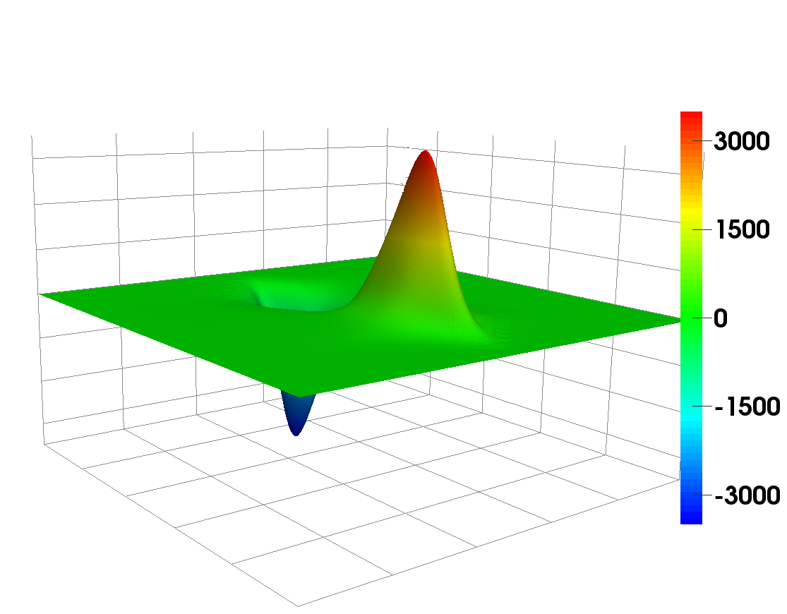
Refer to caption
Refer to caption
Refer to caption
Refer to caption
Refer to caption
Refer to caption
Figure 3: Example 6.1: Surface plot (top) and view from above (bottom) of the analytical solution of (4) at t=t0𝑡subscript𝑡0t=t_{0} (left), t=T/2𝑡𝑇2t=T/2 (middle) and t=T𝑡𝑇t=T (right)

Due to the steep gradients in the neighbourhood of the minimum and maximum, respectively, the use of an adaptive finite element discretization is justified. The resulting computational meshes as well as the corresponding finest mesh (reference mesh at the end of the simulation) are shown in Figure 4. The number of node points of the adaptive meshes varies between 3637 and 7071 points. The finest mesh has 18628 node points. In contrary, a uniform mesh with the same discretization fineness as the finest triangle in the adaptive grids (hmin=0.0047subscript0.0047h_{\min}=0.0047) would have 93025 node points. This clearly reveals the benefit of using adaptive meshes for snapshot generation. Particularly, the comparison of the computational times emphasizes the benefit of adaptive snapshot sampling: the snapshot generation on the adaptive mesh takes 944 seconds, whereas utilizing the uniform mesh it takes 8808 seconds. Therefore, we gain a speedup factor of 9 (see Table 2).
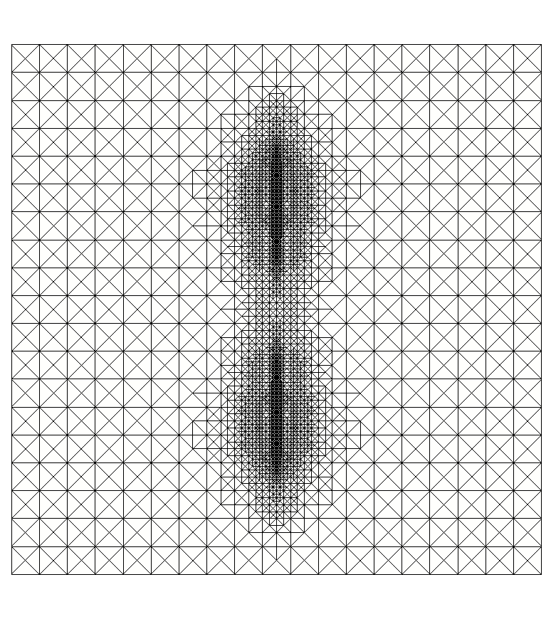
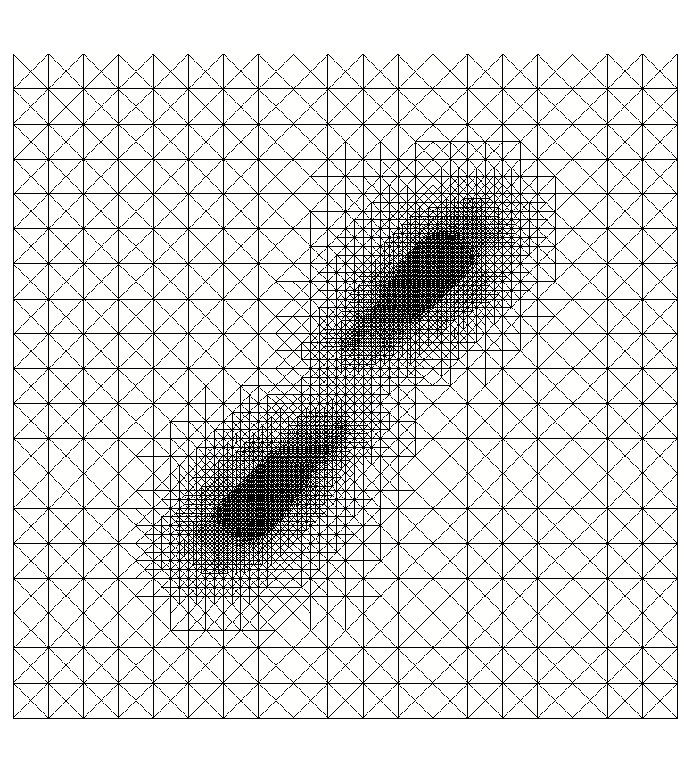
Refer to caption
Refer to caption
Refer to caption
Refer to caption
Figure 4: Example 6.1: Adaptive finite element meshes at t=t0𝑡subscript𝑡0t=t_{0} (left), t=T/2𝑡𝑇2t=T/2 (middle left), t=T𝑡𝑇t=T (middle right) and finest mesh (right)

In Figure 5, the resulting normalized eigenspectrum of the correlation matrix for uniform spatial discretization (“uniform FE mesh”), the normalized eigenspectrum of the matrix 𝒦𝒦\mathcal{K} (16) without interpolation (“infPOD”) as well as the normalized eigenspectrum of the correlation matrix utilizing snapshots interpolated onto the finest mesh (“adaptive FE mesh”) is shown. We observe that the eigenvalues for both adaptive approaches coincide. This numerically validates what we expect from theory: the information content which is contained in the matrix 𝒦𝒦\mathcal{K} when we explicitly compute the entries without interpolation is the same as the information content contained within the eigenvalue problem which is formulated when using the finest mesh. No information is added or lost. Moreover, we recognize that about the first 28 eigenvalues computed corresponding to the adaptive simulation coincide with the simulation on a uniform mesh. From index 29 on, the methods deliver different results: for the uniform discretizations, the normalized eigenvalues fall below machine precision at around index 100 and stagnate. In contrary, the normalized eigenvalues for both adaptive approaches flatten in the order around 1010superscript101010^{-10}. If the error tolerance for the spatial discretization error is chosen larger (or smaller), the stagnation of the eigenvalues in the adaptive method takes place at a higher (or lower) order (see Figure 5, right).
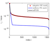
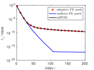
Refer to caption
Refer to caption
Refer to caption
Figure 5: Example 6.1: Comparison of the normalized eigenvalues utilizing an adaptive and a uniform spatial mesh, respectively. Left: all eigenvalues, middle: first 200 largest eigenvalues, right: first 200 largest eigenvalues with different error tolerances for the adaptivity (1.5 times bigger and smaller error tolerances, respectively)

Concerning dynamical systems, the magnitude of the eigenvalue corresponds to the characteristic properties of the underlying dynamical system: the larger the eigenvalue, the more information is contained in the corresponding eigenfunction. Since all adaptive meshes are contained in the uniform mesh, the difference in the amplitude of the eigenvalues is due to the interpolation errors during refinement and coarsening. This is the price we have to pay in order to get a fast snapshot generation utilizing adaptive finite elements. Moreover, the investigation of the decay of the eigenvalues can be interpreted as an analyzing tool for adaptivity in the following sense: Using an adaptive mesh technique means that some parts of the domain are resolved coarsely according to the utilized error estimation, i.e. information gets lost. In the sense of a singular value analysis, this can be explained that adaptivity neglects the noise which is indicated by the singular values on the uniform spatial mesh at those places which are not resolved with the adaptive grid. We conclude that the overtones which get lost in the adaptive computations lie in the same space which is not considered by POD when using the adaptive finite element snapshots. This allows us to characterize the space which is not resolved by adaptivity. From this point of view, adaptivity can be interpreted as a smoother.

Since the first few POD basis functions are the most important ones regarding the captured information, we visualize ψ1,ψ2subscript𝜓1subscript𝜓2\psi_{1},\psi_{2} and ψ5subscript𝜓5\psi_{5} in Figure 6, which are computed corresponding to using an adaptive grid. The POD basis functions corresponding to the uniform spatial discretization have a similar appearance. Note that the POD bases are unique up to the sign. We can recognize the initial condition in the first POD basis function. Then, the index of the POD basis corresponds to the number of maxima and minima of the POD basis: ψ2subscript𝜓2\psi_{2} has two minima and two maxima etc. This behaviour is similar to the increasing oscillations in higher frequencies in trigonometric approximations. The increasing number of oscillations is necessary in order to approximate the transport of the steep gradients of the solution with increasing accuracy.
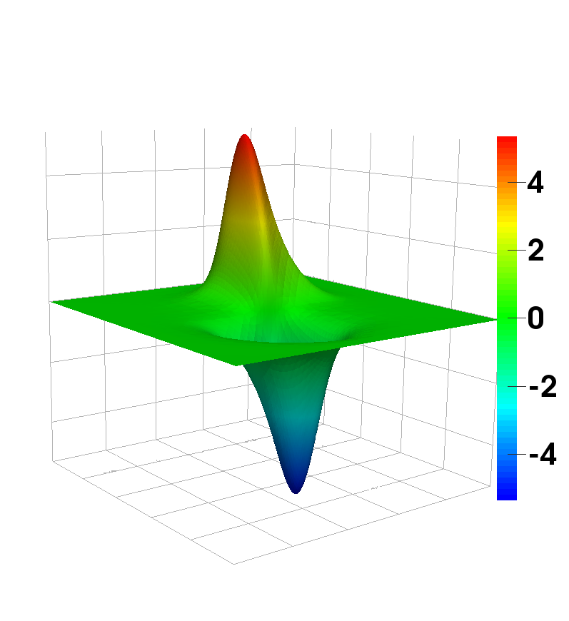
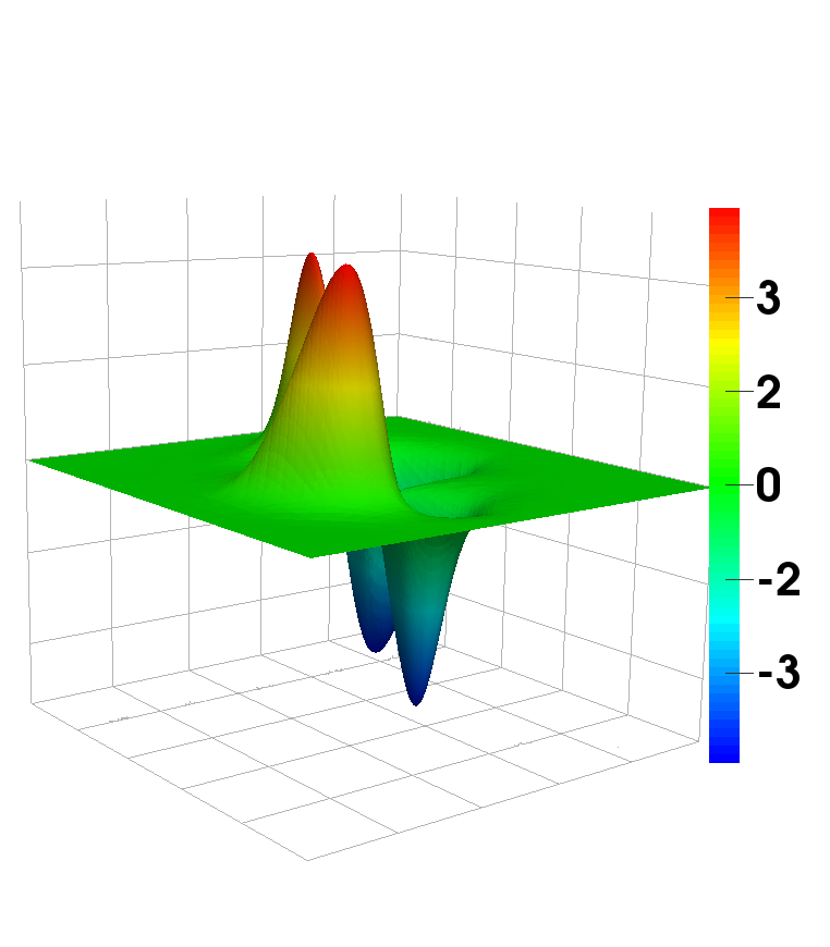
Refer to caption
Refer to caption
Refer to caption
Refer to caption
Refer to caption
Refer to caption
Figure 6: Example 6.1: Surface plot (top) and view from above (bottom) of the POD basis functions ψ1subscript𝜓1\psi_{1} (left), ψ2subscript𝜓2\psi_{2} (middle) and ψ5subscript𝜓5\psi_{5} (right)

The POD solutions for =1010\ell=10 and =5050\ell=50 POD basis functions utilizing spatial adaptive snapshots which are interpolated onto the finest mesh are shown in Figure 7. The visual comparison makes clear what influence the increase of the number of utilized POD basis functions has on the approximation quality. The more POD basis functions we use (until stagnation of the corresponding eigenvalues), the less oscillations appear in the POD solution and the better is the approximation.
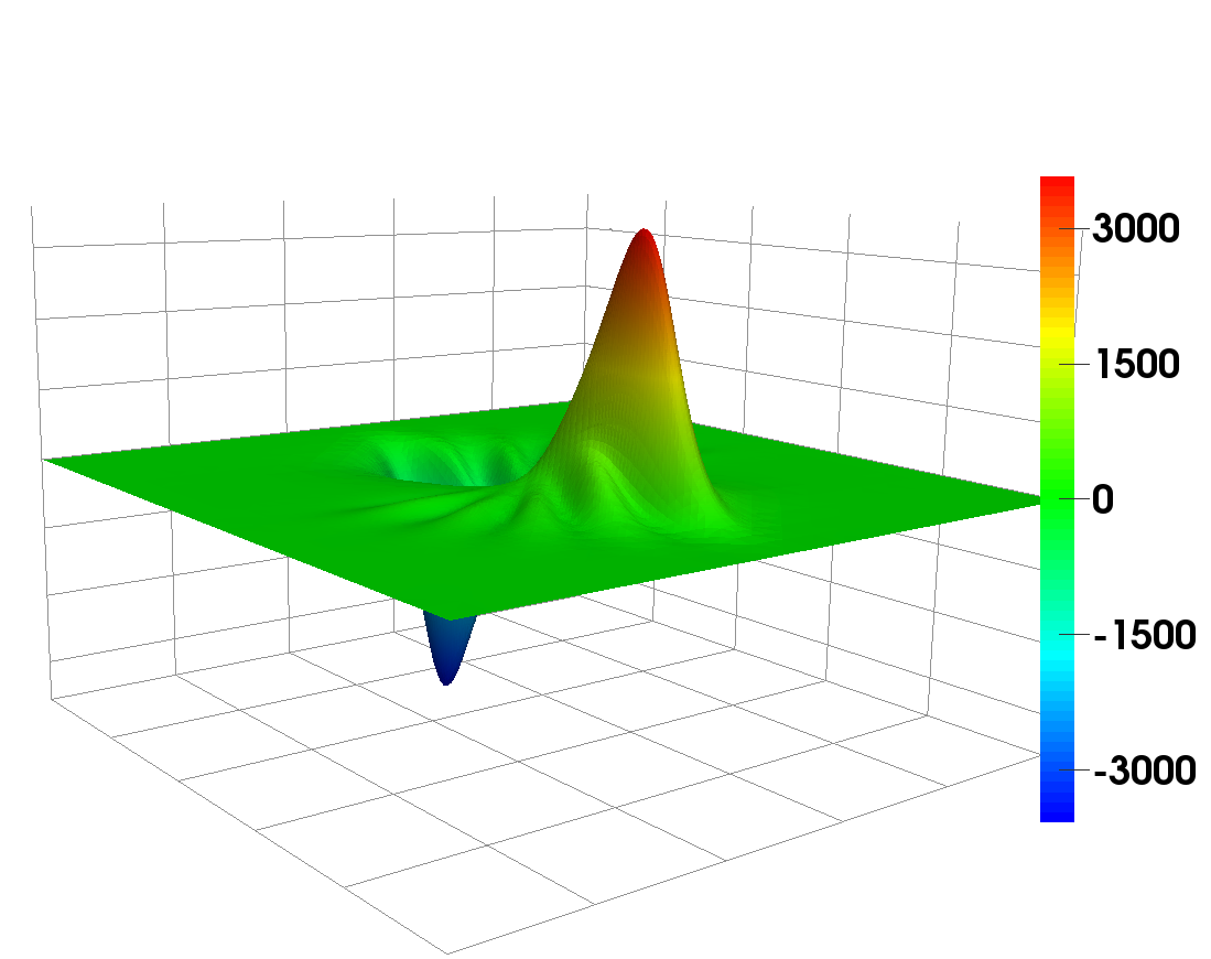
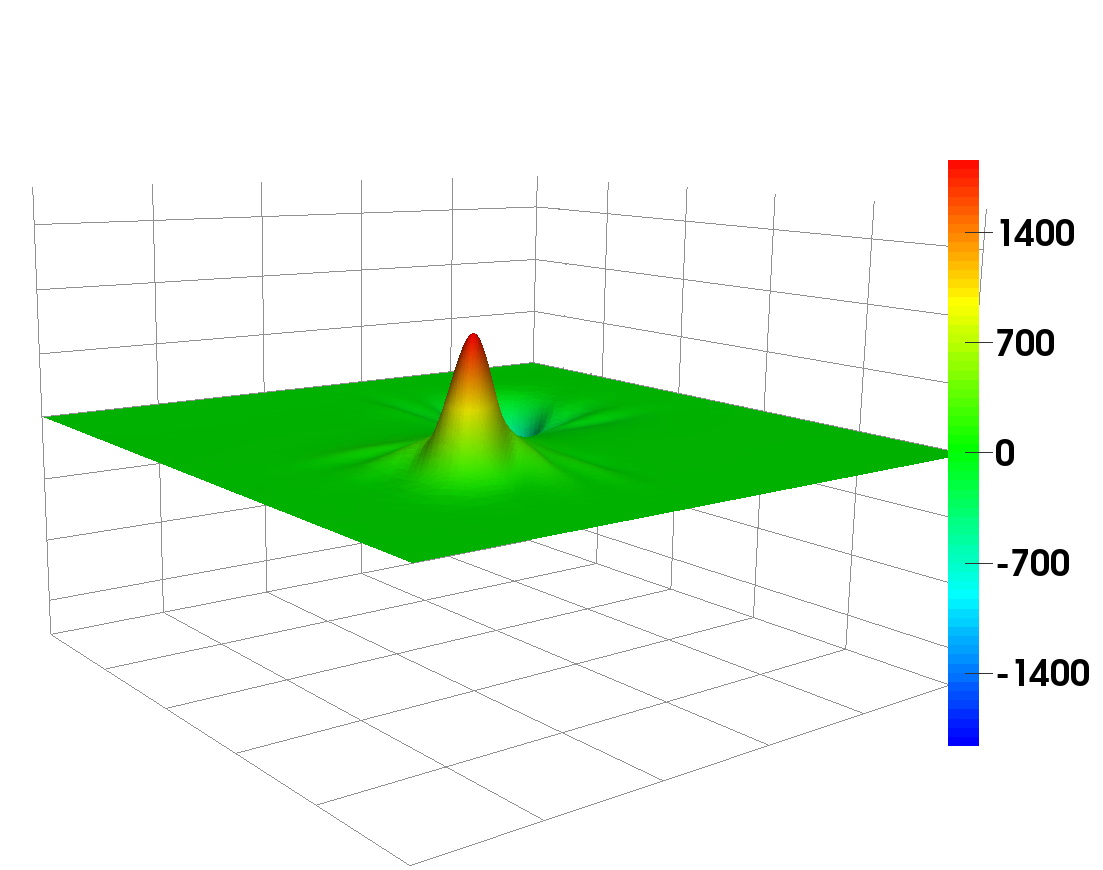
Refer to caption
Refer to caption
Refer to caption
Refer to caption
Refer to caption
Refer to caption
Figure 7: Example 6.1: Surface plot of the POD solution utilizing =1010\ell=10 (top) and =5050\ell=50 (bottom) POD basis functions at t=t0𝑡subscript𝑡0t=t_{0} (left), t=T/2𝑡𝑇2t=T/2 (middle) and t=T𝑡𝑇t=T (right)

Table 1 compares the approximation quality of the POD solution utilizing adaptively generated snapshots which are interpolated onto the finest mesh with snapshots of uniform spatial discretization depending on different POD basis lengths. Our approach from Sections 3 and 4 delivers very similar results as the use of adaptive finite element snapshots which are interpolated onto the finest mesh. For example, for =2020\ell=20 POD bases, we get the following errors: relative L2(0,T;L2(Ω))superscript𝐿20𝑇superscript𝐿2ΩL^{2}(0,T;L^{2}(\Omega))-error between the POD solution and the finite element solution: εFE=3.07102subscript𝜀FE3.07superscript102\varepsilon_{\text{FE}}=3.07\cdot 10^{-2}, relative L2(0,T;L2(Ω))superscript𝐿20𝑇superscript𝐿2ΩL^{2}(0,T;L^{2}(\Omega))-error between the POD solution and the true solution: εtrue=2.16102subscript𝜀true2.16superscript102\varepsilon_{\text{true}}=2.16\cdot 10^{-2}.

\ell εFEadsuperscriptsubscript𝜀FEad\varepsilon_{\text{FE}}^{\text{ad}} εFEunisuperscriptsubscript𝜀FEuni\varepsilon_{\text{FE}}^{\text{uni}} εtrueadsuperscriptsubscript𝜀truead\varepsilon_{\text{true}}^{\text{ad}} εtrueunisuperscriptsubscript𝜀trueuni\varepsilon_{\text{true}}^{\text{uni}}
1 1.301001.30superscript1001.30\cdot 10^{0} 1.301001.30superscript1001.30\cdot 10^{0} 1.281001.28superscript1001.28\cdot 10^{0} 1.301001.30superscript1001.30\cdot 10^{0}
3 7.491017.49superscript1017.49\cdot 10^{-1} 7.581017.58superscript1017.58\cdot 10^{-1} 7.461017.46superscript1017.46\cdot 10^{-1} 7.601017.60superscript1017.60\cdot 10^{-1}
5 4.391014.39superscript1014.39\cdot 10^{-1} 4.451014.45superscript1014.45\cdot 10^{-1} 4.391014.39superscript1014.39\cdot 10^{-1} 4.461014.46superscript1014.46\cdot 10^{-1}
10 1.371011.37superscript1011.37\cdot 10^{-1} 1.371011.37superscript1011.37\cdot 10^{-1} 1.361011.36superscript1011.36\cdot 10^{-1} 1.381011.38superscript1011.38\cdot 10^{-1}
20 3.081023.08superscript1023.08\cdot 10^{-2} 1.561021.56superscript1021.56\cdot 10^{-2} 2.171022.17superscript1022.17\cdot 10^{-2} 1.601021.60superscript1021.60\cdot 10^{-2}
30 2.591022.59superscript1022.59\cdot 10^{-2} 2.041032.04superscript1032.04\cdot 10^{-3} 1.491021.49superscript1021.49\cdot 10^{-2} 3.001033.00superscript1033.00\cdot 10^{-3}
50 2.631022.63superscript1022.63\cdot 10^{-2} 5.671055.67superscript1055.67\cdot 10^{-5} 1.411021.41superscript1021.41\cdot 10^{-2} 2.071032.07superscript1032.07\cdot 10^{-3}
100 2.611022.61superscript1022.61\cdot 10^{-2} 6.481086.48superscript1086.48\cdot 10^{-8} 1.401021.40superscript1021.40\cdot 10^{-2} 2.061032.06superscript1032.06\cdot 10^{-3}
150 2.611022.61superscript1022.61\cdot 10^{-2} 8.131078.13superscript1078.13\cdot 10^{-7} 1.391021.39superscript1021.39\cdot 10^{-2} 2.071032.07superscript1032.07\cdot 10^{-3}
Table 1: Example 6.1: Relative L2(0,T;L2(Ω))superscript𝐿20𝑇superscript𝐿2ΩL^{2}(0,T;L^{2}(\Omega))-error between the POD solution and the finite element solution (columns 2-3) and the true solution (columns 4-5), respectively, utilizing adaptive finite element snapshots which are interpolated onto the finest mesh and utilizing a uniform mesh

We note that the error between POD solution and finite element solution utilizing a uniform mesh decays down to the order 108superscript10810^{-8} (=100100\ell=100) and then stagnates. This behaviour is clear, since the more POD basis we include (up to stagnation of the corresponding eigenvalues), the better is the POD solution an approximation for the finite element solution. In contrary, the error between the POD solution and the true solution starts to stagnate from =2929\ell=29. This is due to the fact that at this point the spatial discretization error dominates the modal error. This is in accordance to the decay of the eigenvalues shown in Figure 5. Due to the error estimation (41), the error between the true solution to (3) and the POD reduced order solution is not only bounded by the sum of the neglected eigenvalues, which is small for sufficiently large number of utilized POD modes. It is also restricted by the spatial and temporal discretization error, which leads to a stagnation of the error in Table 1, columns 4 and 5.

Finally, of particular interest is the computational efficiency of the POD reduced order modeling utilizing adaptive finite element discretizations. For this reason, the computational times for the full and the low order simulation utilizing uniform finite element discretizations and adaptive finite element snapshots, which are interpolated onto the finest mesh, respectively, are listed in Table 2.

adaptive FE mesh uniform FE mesh speedup factor
FE simulation 944 sec 8808 sec 9.3
POD offline computations 264 sec 1300 sec 4.9
POD simulation 187 sec
speedup factor 5.0 47.1
Table 2: Example 6.1: CPU times for FE and POD simulation utilizing uniform finite element meshes and adaptive finite element snapshots which are interpolated onto the finest mesh, respectively, and utilizing =5050\ell=50 POD modes

Once the POD basis is computed in the offline phase, the POD simulation corresponding to adaptive snapshots is 5 times faster than the FE simulation utilizing adaptive finite element meshes. This speedup factor even gains greater importance, if we think of optimal control problems, where the repeated solving of several partial differential equations is necessary. In the POD offline phase, the most expensive task is to express the snapshots with respect to the common finite element space, which takes 226 seconds. Since 𝒦𝒦\mathcal{K} is symmetric, it suffices to calculate the entries on and above the diagonal, which are k=1n+1k=12((n+1)2+n+1)superscriptsubscript𝑘1𝑛1𝑘12superscript𝑛12𝑛1\sum_{k=1}^{n+1}k=\frac{1}{2}((n+1)^{2}+n+1) entries. Thus, the computation of each entry in the correlation matrix 𝒦𝒦\mathcal{K} using a common finite element space takes around 0.00018 seconds. We note that in the approach explained in Section 3 and 4, the computation of the matrix 𝒦𝒦\mathcal{K} (16) is expensive. For each entry the calculation time is around 0.03 seconds, which leads to a computation time of around 36997 seconds for the matrix 𝒦𝒦\mathcal{K}. The same effort is needed to build 𝒴𝒜𝒴superscript𝒴𝒜𝒴\mathcal{Y}^{\star}\mathcal{A}\mathcal{Y}. In this case, the offline phase takes therefore around 88271 seconds. For this reason, the approach to interpolate the adaptive generated snapshots onto the finest mesh is computationally more favorable. But since the computation of 𝒦𝒦\mathcal{K} and 𝒴𝒜𝒴superscript𝒴𝒜𝒴\mathcal{Y}^{\star}\mathcal{A}\mathcal{Y} can be parallelized, the offline computation time can be reduced provided that the appropriate hardware is available.

Example 6.2: Cahn-Hilliard system. We consider Example 2.4, (5) of the Cahn-Hilliard equations given in the coupled formulation for the phase field c𝑐c and the chemical potential w𝑤w. The data is chosen as follows: we consider the rectangular domain Ω=(0,1.5)×(0,0.75)Ω01.500.75\Omega=(0,1.5)\times(0,0.75), the end time T=0.025𝑇0.025T=0.025, constant mobility m0.00002𝑚0.00002m\equiv 0.00002 and a constant surface tension σ24.5𝜎24.5\sigma\equiv 24.5. The interface parameter ε𝜀\varepsilon is set to ε=0.02𝜀0.02\varepsilon=0.02, which leads to an interface thickness of about πε0.0628𝜋𝜀0.0628\pi\cdot\varepsilon\approx 0.0628. We utilize the relaxed double obstacle free energy Wsrelsuperscriptsubscript𝑊𝑠relW_{s}^{\text{rel}}, (7) with s=104𝑠superscript104s=10^{4}. As initial condition, we choose a circle with radius r=0.25𝑟0.25r=0.25 and center (0.375,0.375)0.3750.375(0.375,0.375). The initial condition is transported horizontally with constant velocity v=(30,0)T𝑣superscript300𝑇v=(30,0)^{T}. Let us define the uniform time discretization

tj=jΔtsubscript𝑡𝑗𝑗Δ𝑡t_{j}=j\Delta t

for j=0,,1000𝑗01000j=0,\dotsc,1000 with Δt=2.5105Δ𝑡2.5superscript105\Delta t=2.5\cdot 10^{-5}. We utilize a semi-implicit Euler scheme for temporal discretization. Let cj1Vsuperscript𝑐𝑗1𝑉c^{j-1}\in V and cjVsuperscript𝑐𝑗𝑉c^{j}\in V denote the time-discrete solution at tj1subscript𝑡𝑗1t_{j-1} and tjsubscript𝑡𝑗t_{j}. Based on the variational formulation (9) we tackle the time-discrete version of (5) in the form: given cj1superscript𝑐𝑗1c^{j-1}, find cjsuperscript𝑐𝑗c^{j} with associated wjsuperscript𝑤𝑗w^{j} solving

{cjcj1Δt,v1L2+vcj1,v1L2+mwj,v1L2=0v1V,wj,v2L2+σεcj,v2L2+σεW+(cj)+W(cj1),v2L2=0v2V,casessubscriptsuperscript𝑐𝑗superscript𝑐𝑗1Δ𝑡subscript𝑣1superscript𝐿2subscript𝑣superscript𝑐𝑗1subscript𝑣1superscript𝐿2𝑚subscriptsuperscript𝑤𝑗subscript𝑣1superscript𝐿20for-allsubscript𝑣1𝑉subscriptsuperscript𝑤𝑗subscript𝑣2superscript𝐿2𝜎𝜀subscriptsuperscript𝑐𝑗subscript𝑣2superscript𝐿2𝜎𝜀subscriptsubscriptsuperscript𝑊superscript𝑐𝑗subscriptsuperscript𝑊superscript𝑐𝑗1subscript𝑣2superscript𝐿20for-allsubscript𝑣2𝑉\left\{\begin{array}[]{rcll}\langle\displaystyle\frac{c^{j}-c^{j-1}}{\Delta t},v_{1}\rangle_{L^{2}}+\langle v\cdot\nabla c^{j-1},v_{1}\rangle_{L^{2}}+m\langle\nabla w^{j},\nabla v_{1}\rangle_{L^{2}}&=&0&\forall v_{1}\in V,\\ -\langle w^{j},v_{2}\rangle_{L^{2}}+\sigma\varepsilon\langle\nabla c^{j},\nabla v_{2}\rangle_{L^{2}}+\displaystyle\frac{\sigma}{\varepsilon}\langle W^{\prime}_{+}(c^{j})+W^{\prime}_{-}(c^{j-1}),v_{2}\rangle_{L^{2}}&=&0&\forall v_{2}\in V,\\ \end{array}\right. (43)

and c0=c0superscript𝑐0subscript𝑐0c^{0}=c_{0}. According to (9), here it is V={vH1(Ω),1|Ω|Ωv𝑑x=0}𝑉formulae-sequence𝑣superscript𝐻1Ω1ΩsubscriptΩ𝑣differential-d𝑥0V=\{v\in H^{1}(\Omega),\frac{1}{|\Omega|}\int_{\Omega}vdx=0\}. Note that the free energy function W𝑊W is split into a convex part W+subscript𝑊W_{+} and a concave part Wsubscript𝑊W_{-}, such that W=W++W𝑊subscript𝑊subscript𝑊W=W_{+}+W_{-} and W+subscriptsuperscript𝑊W^{\prime}_{+} is treated implicitly with respect to time and Wsubscriptsuperscript𝑊W^{\prime}_{-} is treated explicitly with respect to time. This leads to an unconditionally energy stable time marching scheme, compare [17]. The system (43) is discretized in space utilizing piecewise linear and continuous finite elements and solved using a semi-smooth Newton method.

Figures 8 shows the phase field (left) and the chemical potential (right) for the finite element simulation utilizing adaptive meshes. The initial condition c0subscript𝑐0c_{0} is transported horizontally with constant velocity.
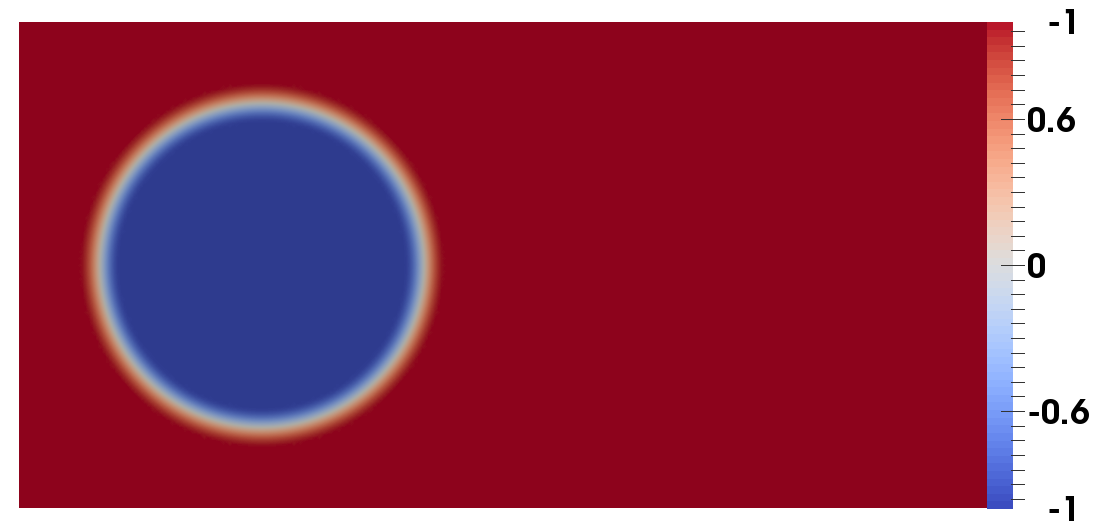
Refer to caption
Refer to caption
Refer to caption
Refer to caption
Refer to caption
Refer to caption
Figure 8: Example 6.2: Phase field c𝑐c (left) and chemical potential w𝑤w (right) computed on adaptive finite element meshes at t=t0𝑡subscript𝑡0t=t_{0} (top), t=T/2𝑡𝑇2t=T/2 (middle) and t=T𝑡𝑇t=T (bottom)

The adaptive finite element meshes as well as the finest mesh which is generated during the adaptive finite element simulation are shown in Figure 9. The number of degrees of freedom in the adaptive meshes varies between 6113 and 8795. The finest mesh (overlay of all adaptive meshes) has 54108 degrees of freedom, whereas a uniform mesh with discretization fineness as small as the smallest triangle in the adaptive meshes has 88450 degrees of freedom.
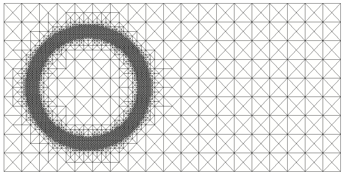
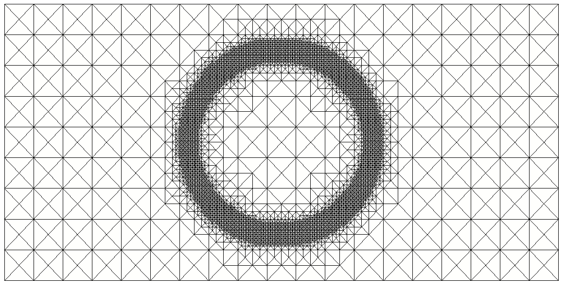
Refer to caption
Refer to caption
Refer to caption
Refer to caption
Figure 9: Example 6.2: Adaptive finite element meshes and finest mesh

In this example, we only compare the solution to the POD-ROM utilizing two kinds of snapshot discretizations: on the one hand we use adaptive finite elements and express these with respect to the finite element basis functions corresponding to the finest mesh. On the other hand we compute the solution to the POD-ROM with snapshots computed on a uniform finite element discretization, where the fineness is chosen to be of the same size as the smallest triangle in the adaptive meshes. We choose X=L2(Ω)𝑋superscript𝐿2ΩX=L^{2}(\Omega) and compute a separate POD basis for each of the variables c𝑐c and w𝑤w.

In Figure 10, a comparison is visualized concerning the normalized eigenspectrum for the phase field c𝑐c and the chemical potential w𝑤w utilizing uniform and adaptive finite element discretization. We note for the phase field c𝑐c that about the first 180 eigenvalues computed corresponding to the adaptive simulation coincide with the eigenvalues of the simulation on the finest mesh. Then, the eigenvalues corresponding to the uniform simulation decay faster. Similar observations apply for the chemical potential w𝑤w.

Refer to caption
Refer to caption
Figure 10: Example 6.2: Comparison of the normalized eigenvalues for the phase field c𝑐c (left) and the chemical potential w𝑤w (right) utilizing an adaptive and a uniform spatial mesh, respectively

In order to control the accuracy of the POD-ROM, we utilize the following criterion. The information content of a POD basis of rank \ell relatively to the amount of the information content of all snapshots is given by the ratio of modeled information and total information. It is defined by

Γ():=i=1λii=1dλi.assignΓsuperscriptsubscript𝑖1subscript𝜆𝑖superscriptsubscript𝑖1𝑑subscript𝜆𝑖\Gamma(\ell):=\displaystyle\frac{\sum_{i=1}^{\ell}\lambda_{i}}{\sum_{i=1}^{d}\lambda_{i}}. (44)

We will choose the POD basis length csubscript𝑐\ell_{c} for the phase field c𝑐c and the number of POD modes wsubscript𝑤\ell_{w} for the chemical potential, such that

min=argmin{Γ():Γ()>1p},with =c and w, respectively,formulae-sequencesubscriptargminconditional-setΓΓ1𝑝with subscript𝑐 and subscript𝑤 respectively,\ell_{\min}=\text{argmin}\{\Gamma(\ell):\Gamma(\ell)>1-p\},\quad\text{with }\ell=\ell_{c}\text{ and }\ell_{w},\text{ respectively,}

for a given value p𝑝p representing the loss of information. Alternatively, one can choose the POD basis length such that the POD projection error (18) is smaller or equal to min((Δt)2,εh2)superscriptΔ𝑡2superscriptsubscript𝜀2\min((\Delta t)^{2},\varepsilon_{h}^{2}), compare (41). Table 3 summarizes how to choose csubscript𝑐\ell_{c} and wsubscript𝑤\ell_{w} in order to capture a desired amount of information. Moreover, it tabulates the POD projection error (18) depending on the POD basis length, where λicsuperscriptsubscript𝜆𝑖𝑐\lambda_{i}^{c} and λiwsuperscriptsubscript𝜆𝑖𝑤\lambda_{i}^{w} denote the eigenvalues for the phase field c𝑐c and the chemical potential w𝑤w, respectively. The results in Table 3 agree with our expectations: the smaller the loss of information p𝑝p is, the more POD modes are needed and the smaller is the POD projection error.

p𝑝p cadsuperscriptsubscript𝑐ad\ell_{c}^{\text{ad}} i=+1dλicsuperscriptsubscript𝑖1𝑑superscriptsubscript𝜆𝑖𝑐\sum_{i=\ell+1}^{d}\lambda_{i}^{c} wadsuperscriptsubscript𝑤ad\ell_{w}^{\text{ad}} i=+1dλiwsuperscriptsubscript𝑖1𝑑superscriptsubscript𝜆𝑖𝑤\sum_{i=\ell+1}^{d}\lambda_{i}^{w} cunisuperscriptsubscript𝑐uni\ell_{c}^{\text{uni}} i=+1dλicsuperscriptsubscript𝑖1𝑑superscriptsubscript𝜆𝑖𝑐\sum_{i=\ell+1}^{d}\lambda_{i}^{c} wunisuperscriptsubscript𝑤uni\ell_{w}^{\text{uni}} i=+1dλiwsuperscriptsubscript𝑖1𝑑superscriptsubscript𝜆𝑖𝑤\sum_{i=\ell+1}^{d}\lambda_{i}^{w}
1001superscript100110^{-01} 3 2.01032.0superscript1032.0\cdot 10^{-3} 4 156.9100156.9superscript100156.9\cdot 10^{0} 3 2.01032.0superscript1032.0\cdot 10^{-3} 4 157.6100157.6superscript100157.6\cdot 10^{0}
1002superscript100210^{-02} 10 2.11042.1superscript1042.1\cdot 10^{-4} 13 15.810015.8superscript10015.8\cdot 10^{0} 10 2.11042.1superscript1042.1\cdot 10^{-4} 13 15.610015.6superscript10015.6\cdot 10^{0}
1003superscript100310^{-03} 19 2.51052.5superscript1052.5\cdot 10^{-5} 26    1.81001.8superscript1001.8\cdot 10^{0} 19 2.51052.5superscript1052.5\cdot 10^{-5} 25    1.81001.8superscript1001.8\cdot 10^{0}
1004superscript100410^{-04} 29 2.01062.0superscript1062.0\cdot 10^{-6} 211      1.81011.8superscript1011.8\cdot 10^{-1} 28 2.61062.6superscript1062.6\cdot 10^{-6} 160      1.91011.9superscript1011.9\cdot 10^{-1}
1005superscript100510^{-05} 37 2.51072.5superscript1072.5\cdot 10^{-7} 644      1.11021.1superscript1021.1\cdot 10^{-2} 37 2.41072.4superscript1072.4\cdot 10^{-7} 419      2.51022.5superscript1022.5\cdot 10^{-2}
Table 3: Example 6.2: Number of needed POD bases in order to achieve a loss of information below the tolerance p𝑝p utilizing adaptive finite element meshes (columns 2-5) and uniform finite element discretization (columns 6-9) and POD projection error

In the following, we run the numerical simulations for different combinations of numbers for csubscript𝑐\ell_{c} and wsubscript𝑤\ell_{w} of Table 3. The approximation quality of the POD solution utilizing adaptive meshes is compared to the use of a uniform mesh in Table 4. As expected, Table 4 shows that the error between the POD surrogate solution and the high-fidelity solution gets smaller for an increasing number of utilized POD basis functions. Moreover, a larger number of POD modes is needed for the chemical potential w𝑤w than for the phase field c𝑐c in order to get an error in the same order which is in accordance to the fact that the decay of the eigenvalues for w𝑤w is slower than for c𝑐c as seen in Figure 10.
Figure 11 visualizes the first, second and fifth POD modes for the phase field c𝑐c and the chemical potential w𝑤w. Analogue to Example 6.1, we observe a periodicity in the POD bases corresponding to its index number.

csuperscript𝑐\ell^{c} wsuperscript𝑤\ell^{w} c:εFEad:𝑐superscriptsubscript𝜀FEadc:\varepsilon_{\text{FE}}^{\text{ad}} w:εFEad:𝑤superscriptsubscript𝜀FEadw:\varepsilon_{\text{FE}}^{\text{ad}} c:εFEuni:𝑐superscriptsubscript𝜀FEunic:\varepsilon_{\text{FE}}^{\text{uni}} w:εFEuni:𝑤superscriptsubscript𝜀FEuniw:\varepsilon_{\text{FE}}^{\text{uni}}
3 4 8.441038.44superscript1038.44\cdot 10^{-3} 3.001003.00superscript1003.00\cdot 10^{0} 8.441038.44superscript1038.44\cdot 10^{-3} 3.751003.75superscript1003.75\cdot 10^{0}
10 13 3.301033.30superscript1033.30\cdot 10^{-3} 3.771013.77superscript1013.77\cdot 10^{-1} 3.301033.30superscript1033.30\cdot 10^{-3} 4.321014.32superscript1014.32\cdot 10^{-1}
19 26 1.571031.57superscript1031.57\cdot 10^{-3} 2.121012.12superscript1012.12\cdot 10^{-1} 1.571031.57superscript1031.57\cdot 10^{-3} 2.391012.39superscript1012.39\cdot 10^{-1}
29 26 7.341047.34superscript1047.34\cdot 10^{-4} 1.091011.09superscript1011.09\cdot 10^{-1} 7.321047.32superscript1047.32\cdot 10^{-4} 1.161011.16superscript1011.16\cdot 10^{-1}
37 26 3.571043.57superscript1043.57\cdot 10^{-4} 4.821024.82superscript1024.82\cdot 10^{-2} 3.551043.55superscript1043.55\cdot 10^{-4} 5.041025.04superscript1025.04\cdot 10^{-2}
50 50 1.881041.88superscript1041.88\cdot 10^{-4} 2.171022.17superscript1022.17\cdot 10^{-2} 1.861041.86superscript1041.86\cdot 10^{-4} 2.331022.33superscript1022.33\cdot 10^{-2}
65 26 9.741059.74superscript1059.74\cdot 10^{-5} 1.111021.11superscript1021.11\cdot 10^{-2} 9.561059.56superscript1059.56\cdot 10^{-5} 1.151021.15superscript1021.15\cdot 10^{-2}
100 100 3.371053.37superscript1053.37\cdot 10^{-5} 3.561033.56superscript1033.56\cdot 10^{-3} 3.221053.22superscript1053.22\cdot 10^{-5} 3.421033.42superscript1033.42\cdot 10^{-3}
Table 4: Example 6.2: Relative L2(0,T;L2(Ω))superscript𝐿20𝑇superscript𝐿2ΩL^{2}(0,T;L^{2}(\Omega))-error between the POD solution and the finite element solution utilizing adaptive meshes (columns 3-4) and utilizing a uniform mesh (columns 5-6), respectively.
Refer to caption
Refer to caption
Refer to caption
Refer to caption
Refer to caption
Refer to caption
Figure 11: Example 6.2: First, second and fifth POD bases for c𝑐c (left) and w𝑤w (right).

Finally, the treatment of the nonlinearity shall be discussed. Utilizing the convex-concave splitting for W𝑊W, we get for the Moreau-Yosida relaxed double obstacle free energy Wrel(c)=12(1c2)superscriptsubscript𝑊rel𝑐121superscript𝑐2W_{-}^{\text{rel}}(c)=\frac{1}{2}(1-c^{2}) for the concave part and W+rel(c)=s2(max(c1,0)2+min(c+1,0)2)W_{+}^{\text{rel}}(c)=\frac{s}{2}(\max(c-1,0)^{2}+\min(c+1,0)^{2}) for the convex part. This means that the first derivative of the concave part is linear with respect to the phase field variable c𝑐c. The challenging part is the convex term which first derivative is non-smooth. For a comparison, we consider the smooth polynomial free energy which concave part is Wp(c)=14(12c2)superscriptsubscript𝑊𝑝𝑐1412superscript𝑐2W_{-}^{p}(c)=\frac{1}{4}(1-2c^{2}) and convex part is W+p(c)=14c4superscriptsubscript𝑊𝑝𝑐14superscript𝑐4W_{+}^{p}(c)=\frac{1}{4}c^{4}.
Figure 12 shows the decay of the normalized eigenspectrum for the phase field c𝑐c (left) and the first derivative of the convex part W+(c)subscriptsuperscript𝑊𝑐W^{\prime}_{+}(c) (right) for the polynomial and the relaxed double obstacle free energy. Obviously, in the non-smooth case more POD modes are needed for a good approximation than in the smooth case. This behaviour is similar to the decay of the Fourier coefficients in the context of trigonometric approximation, where the decay of the Fourier coefficients depends on the smoothness of the approximated object.
Table 5 summarizes computational times for different finite element runs as well as reduced order simulations utilizing the polynomial and the relaxed double obstacle free energy, respectively. In addition, the approximation quality is compared. The computational times are rounded averages from various test runs. It turns out that the finite element simulation (row 1) using the smooth potential is around two times faster than using the non-smooth potential. This is due to
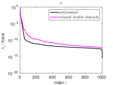
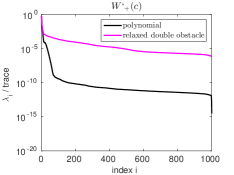
Refer to caption
Refer to caption
Figure 12: Example 6.2: Comparison of the normalized eigenvalues for c𝑐c (left) and the first derivative of the convex part W+subscriptsuperscript𝑊W^{\prime}_{+} of the free energy (right) utilizing polynomial and relaxed double obstacle energy, respectively
Wpsuperscript𝑊𝑝W^{p} Wsrelsuperscriptsubscript𝑊𝑠relW_{s}^{\text{rel}}
FE 1644 sec 3129 sec
c=3,w=4formulae-sequencesubscript𝑐3subscript𝑤4\ell_{c}=3,\ell_{w}=4 c=19,w=26formulae-sequencesubscript𝑐19subscript𝑤26\ell_{c}=19,\ell_{w}=26 c=3,w=4formulae-sequencesubscript𝑐3subscript𝑤4\ell_{c}=3,\ell_{w}=4 c=19,w=26formulae-sequencesubscript𝑐19subscript𝑤26\ell_{c}=19,\ell_{w}=26
POD offline 355 sec 355 sec 350 sec 349 sec
DEIM offline 8 sec 8 sec 9 sec 10 sec
ROM 183 sec 191 sec 2616 sec 3388 sec
ROM-DEIM 0.05 sec 0.1 sec 0.04 sec no conv.
ROM-proj 0.008 sec 0.03 sec 0.01 sec 0.03 sec
speedup FE-ROM 8.9 8.6 1.1 none
speedup FE-ROM-DEIM 32880 16440 78225
speedup FE-ROM-proj 205500 54800 312900 104300
rel L2(Q)superscript𝐿2𝑄L^{2}(Q) error ROM 5.4610035.46superscript10035.46\cdot 10^{-03} 3.2310043.23superscript10043.23\cdot 10^{-04} 8.4410038.44superscript10038.44\cdot 10^{-03} 1.5710031.57superscript10031.57\cdot 10^{-03}
rel L2(Q)superscript𝐿2𝑄L^{2}(Q) error ROM-DEIM 1.4610021.46superscript10021.46\cdot 10^{-02} 3.8310043.83superscript10043.83\cdot 10^{-04} 8.8410038.84superscript10038.84\cdot 10^{-03}
rel L2(Q)superscript𝐿2𝑄L^{2}(Q) error ROM-proj 4.7010024.70superscript10024.70\cdot 10^{-02} 4.1810024.18superscript10024.18\cdot 10^{-02} 8.7210038.72superscript10038.72\cdot 10^{-03} 9.8010039.80superscript10039.80\cdot 10^{-03}
Table 5: Example 6.2: Computational times, speedup factors and approximation quality for different POD basis lengths and using different free energy potentials

the fact that in the smooth case, 2-3 Newton steps are needed for convergence in each time step, whereas in the non-smooth case 6-8 iterations are needed in the semismooth Newton method.
Utilizing the smooth polynomial free energy, the reduced order simulation is 8-9 times faster than the finite element simulation, whereas utilizing the relaxed double obstacle free energy only delivers a very small speedup. The inclusion of DEIM (we use deim=csubscriptdeimsubscript𝑐\ell_{\text{deim}}=\ell_{c}) in the reduced order model leads to immense speedup factors for both free energy functions (row 8). This is due to the fact that the evaluation of the nonlinearity in the reduced order model is still dependent on the full spatial dimension and hyper reduction methods are necessary for useful speedup factors. Note that the speedup factors are of particular interest in the context of optimal control problems. At the same time, the relative L2(0,T;L2(Ω))superscript𝐿20𝑇superscript𝐿2ΩL^{2}(0,T;L^{2}(\Omega))-error between the finite element solution and the ROM-DEIM solution is close to the quality of the reduced order model solution (row 10-11).
However, in the case of the non-smooth free energy function utilizing c=19subscript𝑐19\ell_{c}=19 POD modes for the phase field and w=26subscript𝑤26\ell_{w}=26 POD modes for the chemical potential, the inclusion of DEIM has the effect that the semismooth Newton method does not converge. For this reason, we treat the nonlinearity by applying the technique explained in Section 4.2., i.e. we project the finite element snapshots for W+(c)subscriptsuperscript𝑊𝑐W^{\prime}_{+}(c) (which are interpolated onto the finest mesh) onto the POD space. Since this leads to linear systems, the computational times are very small (row 6). The error between the finite element solution and the reduced order solution utilizing projection of the nonlinearity lies in the area 1002/1003superscript1002superscript100310^{-02}/10^{-03}. Depending on the motivation, this approximation quality might be sufficient. Nevertheless, we note that that for large numbers of POD modes, utilizing the projection of the nonlinearity onto the POD space leads to a large increase of the error.

Example 6.3: Linear heat equation (revisited).

Like in Example 6.1, let us consider again Example 2.3 (4) of a heat equation with c0𝑐0c\equiv 0 . The purpose of this example is to confirm the numerical applicability of the strategy described in Section 3.2. We set up the matrix 𝒦𝒦\mathcal{K} for snapshots given on non-nested spatial discretization which requires the integration over cut elements. The data is chosen as follows: we consider homogeneous Dirichlet boundary conditions. As spatial domain we choose Ω=[0,1]×[0,1]2Ω0101superscript2\Omega=[0,1]\times[0,1]\subset\mathbb{R}^{2}, the time interval is [0,T]=[0,1]0𝑇01[0,T]=[0,1], and we utilize a uniform temporal discretization with time step size Δt=0.01Δ𝑡0.01\Delta t=0.01. We construct an example such that the analytical solution is known. It is given by

y(t,x)=sin(πx0)sin(πx1)cos(2πtx0).𝑦𝑡𝑥𝜋subscript𝑥0𝜋subscript𝑥12𝜋𝑡subscript𝑥0y(t,x)=\sin(\pi x_{0})\cdot\sin(\pi x_{1})\cdot\cos(2\pi tx_{0}).

The source term f𝑓f and the initial condition g𝑔g are chosen accordingly. The initial condition is discretized using piecewise linear and continuous finite elements on a uniform spatial mesh which is shown in Figure 13 (left). Then, at each time step, the mesh is disturbed by relocating each mesh node according to the assignment

x0x0+θx0(x01)(Δt/10),x1x1+θ0.5x1(x11)(Δt/10),subscript𝑥0subscript𝑥0𝜃subscript𝑥0subscript𝑥01Δ𝑡10subscript𝑥1subscript𝑥1𝜃0.5subscript𝑥1subscript𝑥11Δ𝑡10\begin{array}[]{r c l}x_{0}&\leftarrow&x_{0}+\theta\cdot x_{0}\cdot(x_{0}-1)\cdot(\Delta t/10),\\ x_{1}&\leftarrow&x_{1}+\theta\cdot 0.5\cdot x_{1}\cdot(x_{1}-1)\cdot(\Delta t/10),\end{array}

where θ+𝜃subscript\theta\in\mathbb{R}_{+} is sufficiently small such that all coordinates of the inner node points fulfill 0<x0<10subscript𝑥010<x_{0}<1 and 0<x1<10subscript𝑥110<x_{1}<1. After relocating the mesh nodes, the heat equation is solved on this mesh for the next time instance. For this, we use the Lagrange interpolation in order to interpolate the finite element solution of the previous time step onto the new mesh. The disturbed meshes at t=0.5𝑡0.5t=0.5 and t=1.0𝑡1.0t=1.0 as well as an overlap of two meshes are shown in Figure 13. We follow the strategy explained in Section 3.2 and compute the matrix 𝒦𝒦\mathcal{K} from (16) by evaluating the inner products of the snapshots, where we need to integrate over cut elements.
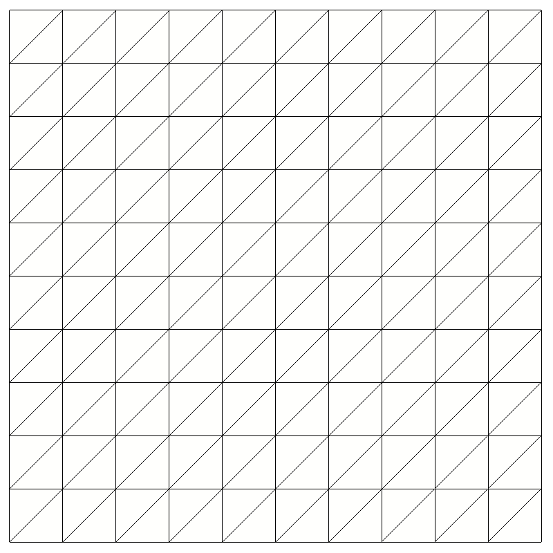
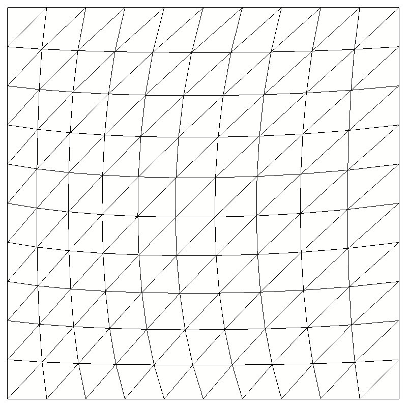
Refer to caption
Refer to caption
Refer to caption
Refer to caption
Figure 13: Example 6.3: Uniform mesh (left), disturbed meshes at t=0.5𝑡0.5t=0.5 and t=1.0𝑡1.0t=1.0 (middle left, middle right), overlap of the mesh at t=0𝑡0t=0 with the mesh at t=1.0𝑡1.0t=1.0 (right). Here, we use θ=10𝜃10\theta=10.

We compute the eigenvalue decomposition of 𝒦𝒦\mathcal{K} for different values of θ𝜃\theta and compare the results with a uniform mesh (i.e. θ=0𝜃0\theta=0) in Figure 14. We note that the eigenvalues of the disturbed mesh are converging to the eigenvalues of the uniform mesh for θ0𝜃0\theta\to 0. As expected, the eigenvalue spectrum depends only weakly on the underlying mesh given that the mesh size is sufficiently small. The POD-ROM follows along the lines of Examples 6.1 and 6.2.
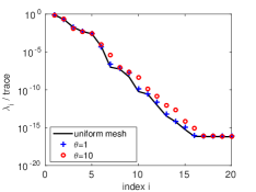
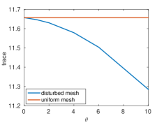
Refer to caption
Refer to caption
Figure 14: Example 6.3: Decay of eigenvalues of matrix 𝒦𝒦\mathcal{K} with different meshes

Our last remark concerns the computational complexity. Solving the heat equation takes 2.1sec on the disturbed meshes and 1.8sec on the uniform mesh. The computational time for each entry of the matrix 𝒦𝒦\mathcal{K} is 0.022sec and computing the eigenvalue decomposition for 𝒦𝒦\mathcal{K} takes 0.0056sec. Note that the cut element integration problem for each matrix entry takes a fraction of time required to solve the finite element problem.

7 Conclusion

In this work, a POD reduced order model is proposed which can be set up and solved for snapshots which are discretized utilizing arbitrary finite elements. The method is applicable for hh-, p𝑝p- and r𝑟r-adaptive finite elements. The approach is motivated from an infinite-dimensional perspective. Using the method of snapshots we are able to set up the correlation matrix by evaluating the inner products of snapshots which live in different finite element spaces. For non-nested meshes, this requires the detection of cell collision and integration over cut finite elements. A numerical strategy how to implement this practically is elaborated and numerically tested. Utilizing the eigenvalues and eigenvectors of this correlation matrix, we are able to set up and solve a POD surrogate model that does not need the expression of the snapshots with respect to the basis of a common finite element space or the interpolation onto a common reference mesh. Moreover, an error bound for the error between the true solution and the solution to the POD-ROM using spatially adapted snapshots is derived. The error estimation contains an additional term according to the spatial discretization error compared to existing error bounds. The numerical tests show that the POD projection error decreases if the number of utilized POD basis functions is increased. However, the error between the POD solution and the true solution stagnates when the spatial discretization error dominates. Moreover, the numerics show that utilizing the correlation matrix calculated explicitly without interpolation in order to build a POD-ROM gives the same results as the approach in which the snapshots are interpolated onto the finest mesh. From a computational point of view, sufficient hardware should be available in order to compute the correlation matrix in parallel and make the offline computational time competitive. For semilinear evolution problems, the nonlinearity is treated by linearization. This is of interest in view of optimal control problems, in which a linearized state equation has to be solved in each SQP iteration level. In future work, we intend to study the combination of adaptive finite elements and POD reduced order modeling in the context of multi-phase flow and optimal control.

References

  • [1] H. Abels. Diffuse Interface Models for Two-Phase flows of Viscous Incompressible Fluids. Max-Planck Institut für Mathematik in den Naturwissenschaften, Leipzig, Lecture Note, 36, 2007.
  • [2] H. Abels, H. Garcke, G. Grün. Thermodynamically consistent, frame indifferent diffuse interface models for incompressible two-phase flows with different densities. Mathematical Models and Methods in Applied Sciences, 22(3):40, 2012.
  • [3] K. Afanasiev, M. Hinze. Adaptive control of a wake flow using proper orthogonal decomposition. Shape optimization and optimal design (Cambridge, 1999), Lecture Notes in Pure and Appl. Math., 216:317-332. Dekker, New York, 2001.
  • [4] M. Ainsworth, J. T. Oden. A posteriori error estimation in finite element analysis. John Wiley & Sons, 37, 2011.
  • [5] M. Ali, K. Steih, K. Urban. Reduced basis methods based upon adaptive snapshot computations. Advances in Computational Mathematics, 43(2):257-294, 2017.
  • [6] A. Alla, J. N. Kutz. Nonlinear model order reduction via Dynamic Mode Decomposition. to appear SIAM Journal on Scientific Computing, 2016.
  • [7] M.S. Alnaes, J. Blechta, J. Hake, A. Johansson, B. Kehlet, A. Logg, C. Richardson, J. Ring, M.E. Rognes, G.N. Wells The FEniCS Project Version 1.5. Archive of Numerical Software, 100(3):9-23, 2015.
  • [8] P. Astrid, S. Weiland, K. Willcox, T. Backx. Missing Point Estimation in Models Described by Proper Orthogonal Decompostion. IEE Trans. Automat. Control, 53(10), 2237-2251, 2008.
  • [9] J. F. Blowey, C. M. Elliott. The Cahn-Hilliard gradient theory for phase separation with non-smooth free energy. Part I: Mathematical analysis. European Journal of Applied Mathematics, 2:233-280, 1991.
  • [10] M. Barrault, Y. Maday, N. C. Nguyen, A. T. Patera. An “empirical interpolation” method: application to efficient reduced-basis discretization of partial differential equations. C. R. Acad. Sci. Paris, Ser. I 339, 667-672, 2004.
  • [11] P. Benner, R. Rannacher. Introduction to Part III Adaptivity and Model Reduction. Trends in PDE Constrained Optimization, International Series of Numerical Mathematics, 165:249-250, 2014.
  • [12] Y. Chen. Model order reduction for nonlinear systems. Master’s thesis, Massachusetts Institute of Technology, 1999.
  • [13] L. Chen. An Innovative Finite Element Method Package in Matlab. Available at ifem.wordpress.com, 2008.
  • [14] J. W. Cahn, J. E. Hilliard. Free energy of a non-uniform system. I. Interfacial free energy. J. Chem. Phys. 28:258-267, 1958.
  • [15] S. Chaturantabut, D. C. Sorensen. Nonlinear model reduction via discrete empirical interpolation. Siam J. Sci. Comput. 32(5), 2737-2764, 2010.
  • [16] Z. Drmac, S. Gugercin. A New Selection Operator for the Discrete Empirical Interpolation Method – improved a priori error bound and extension. SIAM J. Sci. Comput. 38(2):A631-A648, 2016.
  • [17] D. J. Eyre. Unconditionally Gradient Stable Time Marching the Cahn-Hilliard Equation. MRS Proceedings, 529, 1998.
  • [18] F. Fang, C. C. Pain, I. M. Navon, M. D. Piggott, G. J. Gorman, P. A. Allison, A. J. Goddard. Reduced-order modelling of an adaptive mesh ocean model. Int. J. Numer. Meth. Fluids 59: 827-851, 2009.
  • [19] L. Feng, X. Zeng, C. Chiang, D. Zhou, Q. Fang. Direct Nonlinear Order Reduction with Variational Analysis. Proc. Design, Automation and Test in Europe, 1530-1591, 2004.
  • [20] M. Gubisch, S. Volkwein. Proper Orthogonal Decomposition for Linear-Quadratic Optimal Control. In P. Benner, A. Cohen, M. Ohlberger, K. Willcox (eds.), Model Reduction and Approximation: Theory and Algorithms, 5-66, SIAM, Philadelphia, PA, 2017.
  • [21] P. C. Hohenberg, B. I. Halperin. Theory of dynamic critical phenomena. Reviews of Modern Physics, 49(3):435-479, 1977.
  • [22] M. Hintermüller, M. Hinze, M. H. Tber. An Adaptive Finite Element Moreau-Yosida-Based Solver for a Non-Smooth Cahn-Hilliard Problem. Optim. Meth. Software 26:777-811, 2011.
  • [23] M. Hinze, K. Kunisch. Three control methods for time-dependent fluid flow. Flow, Turbulence and Combustion, 65:273-298, 2000.
  • [24] M. Hinze, J. Krenciszek, R. Pinnau. Proper Orthogonal Decomposition for Free Boundary Value Problems. Hamburger Beiträge zur Angewandten Mathematik, 2014.
  • [25] P. Holmes, J. L. Lumley, G. Berkooz, C. W. Rowley. Turbulence, Coherent Structures, Dynamical Systems and Symmetry. Cambridge Monographs on Mechanics, Cambridge University Press, 2012.
  • [26] M. Hinze, S. Volkwein. Error estimates for abstract linear-quadratic optimal control problems using proper orthogonal decomposition. Technical Report IMA02-05, KFU Graz, 2005.
  • [27] M. Hinze, R. Pinnau, M. Ulbrich, S. Ulbrich. Optimization with PDE Constraints. Springer-Verlag, Berlin, 2009.
  • [28] K. Kunisch, S. Volkwein. Control of Burgers’ equation by a reduced order approach using proper orthogonal decomposition. Journal on Optimization Theory and Apllications, 102:345-371, 1999.
  • [29] K. Kunisch, S. Volkwein. Galerkin Proper Orthogonal Decomposition Methods for Parabolic Problems. Numer. Math. 90:117-148, 2001.
  • [30] K. Kunisch, S. Volkwein. Galerkin Proper Orthogonal Decomposition Methods for a General Equation in Fluid Dynamics. SIAM J. Numer. Anal., 40(2):492-515, 2002.
  • [31] O. Lass. Reduced order modeling and parameter identification for coupled nonlinear PDE systems. PhD thesis, Universität Konstanz, 2014.
  • [32] A. Logg, K.-A. Mardal, G. Wells, eds. Automated Solution of Differential Equations by the Finite Element Method. The FEniCS Book, vol. 84 of Lecture Notes in Computational Science and Engineering, Springer, 2012.
  • [33] T. Lassila, A. Manzoni, A. Quarteroni, G. Rozza. Model order reduction in fluid dynamics: challenges and perspectives. Reduced order methods for modeling and computational reduction, A. Quarteroni and G. Rozza, Eds., Springer MS&A Series, 9:235-274, 2014.
  • [34] Y.T. Lee, A.A. Requicha. Algorithms for computing the volume and other integral properties of solids. I. known methods and open issues. Communications of the ACM, 25(9):635-641, 1982.
  • [35] J. L. Lumley. The Structure of Inhomogeneous Turbulent Flows. In A. M. Yaglom and V. I. Tatarski, editors, Atmospheric turbulence and radio propagation, pages 166-178. Nauka, Moscow, 1967.
  • [36] A. Massing, M. Larson, A. Logg. Efficient implementation of finite element methods on nonmatching and overlapping meshes in three dimensions. SIAM Journal on Scientific Computing, 35(1), C.23-C.47, 2013.
  • [37] B. Mirtich Fast and accurate computation of polyhedral mass properties. Journal of graphics tools 1(2):31-50, 1996.
  • [38] N. C. Nguyen, A. T. Patera, J. Peraire. A “best point” interpolation method for efficient approximation of parametrized functions. Int. J. Numer. Meth. Eng., 73(4) 521-543, 2008.
  • [39] A. Pazy. Semigroups of Linear Operators and Applications to Partial Differential Equations. Springer, New York, 1983.
  • [40] J. R. Phillips. Automated extraction of nonlinear circuit macromodels. in Proc. Custom Integrated Circuit Conf., 451-454, 2000.
  • [41] J. R. Phillips. Projection-Based Approaches for Model Reduction of Weakly Nonlinear, Time-Varying Systems. IEE Transactions on computer-aided design of integrated circuits and systems, 22(2), 2003.
  • [42] R. Pinnau. Model Reduction via Proper Orthogonal Decomposition. In W.H.A. Schilder, H. van der Vorst: Model Order Reduction: Theory, Research Aspects and Applications, Springer, 96-109, 2008.
  • [43] J. P. Raymond, H. Zidani. Hamiltonian Pontryagin’s Principles for control problems governed by semilinear parabolic equations. Applied Math. and Optimization, 39:143-177, 1999.
  • [44] M. Reed, B. Simon. Methods of modern mathematical physics. I: Functional analysis. Academic Press 1980.
  • [45] M. Rewieński, J. White. A Trajectory Piecewise-Linear Approach to Model Order Reduction and Fast Simulation of Nonlinear Circuits and Micromachined Devices. IEE Transactions on computer-aided design of integrated circuits and systems, 22(2), 2003.
  • [46] A. Schmidt, K. G. Siebert. Design of adaptive finite element software: The finite element toolbox ALBERTA. Lecture Notes in Computational Science and Engineering, Springer, 42, 2005.
  • [47] J.R. Singler New POD Error Expressions, Error Bounds, and Asymptotic Results for Reduced Order Model of Parabolic PDEs. SIAM Journal on Numerical Analysis, 52(2):852-876, 2014.
  • [48] L. Sirovich. Turbulence and the dynamics of coherent structures. Parts I-II. Quarterly of Applied Mathematics, XVL, 561-590, 1987.
  • [49] S. Ullmann, M. Rotkvic, J. Lang. POD-Galerkin reduced-order modeling with adaptive finite element snapshots. Journal of Computational Physics, 325:244-258, 2016.
  • [50] S. Volkwein. Optimal Control of a Phase-Field Model Using Proper Orthogonal Decomposition. Z. Angew. Math. Mech. 81(2):83-97, 2001.
  • [51] S. Volkwein. Proper Orthogonal Decomposition: Theory and Reduced-Order Modelling. University of Konstanz, Lecture Notes, 2013.
  • [52] Z. Whang. Nonlinear Model Reduction Based on the Finite Element Method With Interpolated Coefficients: Semilinear Parabolic Equations. Numer. Meth. Partial. Diff. Eqs., 31(6):1713-1741, 2015.
  • [53] A. Yagi. Abstract Parabolic Evolution Equations and their Applications. Springer Monographs in Mathematics, 2010.
  • [54] M. Yano. A minimum-residual mixed reduced basis method: Exact residual certification and simultaneous finite-element reduced-basis refinement. ESAIM: M2AN 50(1), 163-185, 2016.