Phase-type Approximation of the Gerber-Shiu Function
Abstract
The Gerber-Shiu function provides a way of measuring the risk of an insurance company. It is given by the expected value of a function that depends on the ruin time, the deficit at ruin, and the surplus prior to ruin. Its computation requires the evaluation of the overshoot/undershoot distributions of the surplus process at ruin. In this paper, we use the recent developments of the fluctuation theory and approximate it in a closed form by fitting the underlying process by phase-type Lévy processes. A sequence of numerical results are given.
Keywords: Risk management, applied probability
1 Introduction
The fundamental objective of the actuarial ruin theory is to measure the vulnerability to insolvency. Typically, the surplus of an insurance company is modeled by a stochastic process, and ruin occurs at the first time it goes below a certain threshold. A most classical and important quantity of interest is the ruin probability, and the Gerber-Shiu function is its generalization; it is given as an expected discounted value of the cost function that is dependent on the ruin time, the deficit at ruin, and the surplus prior to ruin. The evaluation of the Gerber-Shiu function involves that of the overshoot and undershoot distributions at the first down-crossing time that do not admit explicit expressions. Hence its computation is in general a challenging task.
In ruin theory, the surplus process is commonly modeled by a stochastic process with downward jumps. Due to the premiums received from the insured persons, the surplus tends to increase constantly. On the other hand, it experiences sudden downward jumps due to the insurance payments. The classical Cramér-Lundberg model uses a compound Poisson process with downward jumps. Its generalization called the Sparre-Andersen model modifies it by allowing the arrival of the claims to follow a general renewal process.
In the last decade, significant progress has been made in insurance mathematics and ruin theory, thanks to the development of the theory of Lévy processes [9, 19]. In particular, many results on the Cramér-Lundberg model have been generalized for a general spectrally negative Lévy process, or the Lévy process with only downward jumps; see, e.g., [4, 6, 7, 24]. This generalization enables one to construct more realistic models; one can, for example, introduce noise by including Brownian motion and/or infinitesimal jumps of infinite activity/variation. Using the so-called scale function, one can express concisely many quantities of interest for a general spectrally negative Lévy process.
The objective of this paper is to give an approximation to the Gerber-Shiu function using the theory of scale functions. By the compensation formula of the Lévy process, the Gerber-Shiu function admits an expression as a (double) integral with respect to the resolvent measure and the Lévy measure. Because the resolvent can be written using the scale function, at least in theory the computation of the Gerber-Shiu function boils down to that of the scale function.
However, a major obstacle still remains in putting these in practice because scale functions are in general known only up to their Laplace transforms, and only a few cases admit explicit expressions. The most straightforward approach of computing the scale function is to apply numerical Laplace inversion as in [18, 33]. However, this approach is not suitable for the computation of the Gerber-Shiu function because the numerically approximated scale functions need to be further integrated with respect to the Lévy measure. In particular, the undershoot density that is essential in the computation of the Gerber-Shiu function tends to have a very peculiar form with a possible spike. The approximation hence requires a high precision in computing the scale function and minimal discretization errors in numerical integration.
In this paper, we adopt a phase-type fitting of [13] by using the scale function for the class of spectrally negative phase-type Lévy processes, or Lévy processes with negative phase-type-distributed jumps. Consider a continuous-time Markov chain with some initial distribution and state space consisting of a single absorbing state and a finite number of transient states. A phase-type distribution is that of the first entry time to the absorbing state. As has been discussed in [13, 18], the scale function of this process becomes the sum of (possibly complex) exponentials; it can be integrated with respect to the Lévy measure analytically to obtain an explicit form of the Gerber-Shiu function. More importantly, the class of phase-type distributions is dense in the class of all positive-valued distributions. Consequently, the Gerber-Shiu function of any given spectrally negative Lévy process can be approximated in a closed form by that of an approximating spectrally negative phase-type Lévy process. Our aim is to evaluate numerically the practicability of this approach.
In our numerical results, we focus on the case where the Lévy measure is finite and has a completely monotone density. In this case, the jump size distribution can be approximated by a special class of phase-type distributions, called the hyperexponential distributions. While fitting a phase-type distribution for a general distribution is often difficult, fitting a hyperexponential distribution for the ones with completely monotone densities can be efficiently done, for example by the algorithm by [14] that is guaranteed to converge to the desired distribution. The class of Lévy processes with completely monotone Lévy densities includes, for example, a subset of compound Poisson processes, variance gamma [26, 27], CGMY [10], generalized hyperbolic [12] and normal inverse Gaussian [5] processes.
In order to evaluate our approach, we obtain, for the hyperexponential case, the closed-form expressions of the (discounted) overshoot/undershoot distributions at the first down-crossing time, and use it to approximate those for the processes with Weibull/Pareto-type jumps. The obtained results are then compared with those obtained by Monte Carlo simulation.
To our best knowledge, this is the first paper on the numerical evaluation of the Gerber-Shiu function via phase-type fitting. As the Gerber-Shiu measure is sensitive to approximation errors, it is important to evaluate its numerical performance. Recently, the resolvents of related extensions of the Lévy process have been developed, and it is reasonable to conjecture that the Gerber-Shiu function of these can be approximated precisely in the same way.
The rest of the paper is organized as follows. Section 2 reviews the spectrally negative Lévy process, the Gerber-Shiu function, and the scale function. Section 3 gives a summary of [13] on the spectrally negative phase-type Lévy process and its scale function. Section 4 computes the Gerber-Shiu measure of the hyperexponential Lévy process as an approximation for the case the jump size distribution admits a completely monotone density. We evaluate the performance using numerical results in Section 5. Section 6 concludes with remarks on the cases of other variants of spectrally negative Lévy processes.
2 Gerber-Shiu Functions for Spectrally Negative Lévy Processes
Let be a probability space hosting a spectrally negative Lévy process that models the surplus of a company. Let be the conditional probability under which (and also ), and the filtration generated by . The process is uniquely characterized by its Laplace exponent
| (2.1) |
where is the diffusion (Brownian motion) coefficient and is a Lévy measure with the support that satisfies the integrability condition . It has paths of bounded variation if and only if
see, for example, Lemma 2.12 of [19]. In this case, we can rewrite the Laplace exponent (2.1) by
with
We disregard the case when is the negative of a subordinator (or decreasing a.s.).
2.1 Gerber-Shiu functions
Define the ruin time as the first time the surplus goes below zero:
Here and throughout the paper, we use the convention that . On the event , the random variables and model, respectively, the deficit at ruin and surplus immediately before ruin.
Fix bounded and measurable. We define the Gerber-Shiu function
With the Gerber-Shiu measure
we can write
see pages 4 and 5 of [20].
Using the compensation formula (see Theorem 4.4 of [19]), this can be written in terms of the -resolvent measure of killed on exiting :
| (2.2) |
which is known to admit a density for the case of spectrally negative Lévy processes such that
| (2.3) |
see (2.10) below for the form of . As in Section 1.3 of [20], we can write
| (2.4) |
Hence the computation of the Gerber-Shiu measure boils down to that of the resolvent measure.
2.2 Scale functions
In order to compute the resolvent measure (2.2), we shall introduce the scale function.
Fix . The scale function of is a function whose Laplace transform is given by
| (2.5) |
where
| (2.6) |
On the negative half line, it is assumed that .
Regarding the smoothness of the scale function, if the Lévy measure has no atoms or is of unbounded variation, then ; if it has a Gaussian component (), then . See [11] for other known results on the smoothness.
The behavior in the neighborhood of zero is given as follows. As in Lemmas 4.3 and 4.4 of [23], for every ,
| (2.7) | ||||
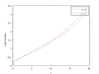
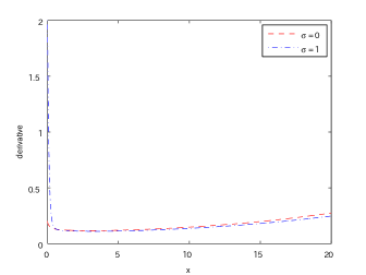
We plot in Figure 1 sample plots of the scale function and its derivative for the bounded variation case with and the unbounded variation case with .
 |
 |
2.3 Resolvent via the scale function
Recall, as in our discussion in Section 2.1, that the Gerber-Shiu function can be written in terms of the resolvent measure. This can be concisely written in terms of the scale function as follows: by Corollary 8.8 of [19], the resolvent density (2.3) can be written
| (2.10) |
Now in view of the identity (2.4), the computation of the Gerber-Shiu measure boils down to that of the scale function.
3 Scale Functions for Spectrally Negative Phase-type Lévy Processes
As discussed in the previous section, the scale function is defined by its Laplace transform and for its computation the Laplace transform (2.5) must be inverted. Here, we review the results on [13] for a special class of Lévy processes where it can be inverted analytically.
3.1 Phase-type distribution
Consider a continuous-time Markov chain
with a finite state space where are transient and is absorbing. Its initial distribution is given by a simplex such that for every . The intensity matrix is partitioned into the transient states and the absorbing state , and is given by
Here is an -matrix called the phase-type-generator, and where . A distribution is called phase-type with representation if it is the distribution of the absorption time to in the Markov chain described above. It is known that is non-singular and thus invertible; see [2]. Its distribution and density functions are given, respectively, by
3.2 Phase-type Lévy processes
Let be a spectrally negative Lévy process of the form
| (3.1) |
for some and (with when so that it is not the negative of a subordinator). Here is a standard Brownian motion, is a Poisson process with arrival rate , and is an i.i.d. sequence of phase-type-distributed random variables with representation . These processes are assumed mutually independent. Its Laplace exponent is then
| (3.2) |
which is analytic for every except at the eigenvalues of .
Let be the set of (the sign-changed) negative roots:
| (3.3) |
where is the real part of . Let denote the number of different roots in and the multiplicity of a root for .
3.3 Approximation results
It is known that the class of phase-type distributions is dense in the class of all positive-valued distributions. Using this, Proposition 1 of [3] shows that, there exists, for any spectrally negative Lévy process , a sequence of spectrally negative phase-type Lévy processes converging to in . In other words, in distribution by Corollary VII 3.6 of [15]; see also [32].
Using these results, Egami and Yamazaki [13] study the convergence of the corresponding scale function, and show that the approximation is in most cases very accurate. On the other hand, as they also point out, no existing algorithm is guaranteed to construct a converging sequences and fitting phase-type distributions can get difficult; see, e.g., the case of fitting for the uniform distributed jump size in [13].
On the other hand, as we shall discuss next, it is guaranteed to work for the case the jump size admits a completely monotone density.
3.4 Hyperexponential case
As an important example where all the roots in are distinct and real, we consider the case where has a hyperexponential distribution with a density function
for some and for such that ; this is the phase-type distribution with its Markov chain such that the transient states are connected only to . Its Laplace exponent (2.1) is then
Notice in this case that , …, are the poles of the Laplace exponent. Furthermore, all the roots in are distinct and real and satisfy the following interlacing condition for every :
-
1.
for , there are roots such that
(3.6) -
2.
for , there are roots such that
(3.7)
Because all roots are real and distinct, the scale function can be written as (3.5).
Recall that a density function of a positive valued random variable is called completely monotone if all the derivatives exist and, for every ,
where denotes the derivative of .
Feldmann and Whitt [14] showed that if a density function is completely monotone, then it can be approximated by those of hyperexponential distributions. As shown by [8], every completely monotone density function is a mixture of exponential density functions, and this implies that, for any distribution with a completely monotone density, there exists a sequence of hyperexponential distributions converging to it. The class of distributions with completely monotone densities contains a number of distributions such as the (subset of) Pareto distribution, the Weibull distribution, and the gamma distribution. Feldmann and Whitt [14] took advantage of this fact and proposed a recursive algorithm for fitting hyperexponential distributions to these distributions. We refer the reader to [1, 17] for other approximation methods.
4 Computation of the Gerber-Shiu Function
We shall now consider the approximation of the Gerber-Shiu function using the fitted scale functions. Here, we consider the hyperexponential case as discussed in Section 3.4; in this case, because the scale function and Lévy measure are both written as mixtures of exponential functions, we attain closed-form expressions.
4.1 Overshoot and undershoot distributions
Recall from (2.4) regarding the equivalence of the Gerber-Shiu measure and the product of the Lévy measure and the resolvent measure. If we define for all and ,
| (4.1) |
Combining (2.4) and (2.10), we can write
where is the Lévy measure of the dual process .
When is a phase-type Lévy process, as we have studied in the previous section can be written as a sum of (possibly complex) exponentials. In particular, if it is hyperexpontial, we can write for all , and hence can be obtained analytically.
Here we assume that is a hyperexponential Lévy process and . The following results are immediate by straightforward integration.
Proposition 4.1.
-
1.
Suppose and for some and . Then
where, for each ,
-
2.
We have
In particular, by setting (),
(4.2) where
5 Numerical Results
Using the identities obtained in Proposition 4.1, we shall evaluate the efficiency of the phase-type fitting approach of the Gerber-Shiu function.
Here we consider the spectrally negative Lévy processes and in the form (3.1) where is
-
(i)
Weibull, and
-
(ii)
Pareto
respectively. Recall that the Weibull distribution with parameters and (denoted Weibull) is give by , , and the Pareto distribution with positive parameters and (denoted Pareto) is given by , . See [16] for more details about these distributions. With the choice of our parameters, the corresponding Lévy densities are thus completely monotone.
As has been noted in Section 3.4, any spectrally negative Lévy process with a completely monotone Lévy density can be approximated arbitrarily closely by fitting hyperexponential distributions. Here, we use the fitted data computed by [14] to approximate the scale function for and (with or without a Brownian motion component). Tables 3 and 9, respectively, of [14] show the parameters of the hyperexponential distributions obtained by [14] fitted to (i) with and to (ii) with . We use these parameters to construct hyperexponential Lévy processes and (see Section 3.4) that will be used to approximate and , respectively.
|
|
||||||||||||||||||||||||||||||||||||||||||||||||||||||||||||||||||||||||
| (i) Weibull | (ii) Pareto |
In order to evaluate the errors associated with the phase-type-fitting of the Gerber-Shiu function, we shall consider approximating the overshoot/undershoot density
for and . The phase-type-fitting approach approximates them by computing those for the approximating hyperexponential Lévy processes and . These can be done analytically by the identity (4.2).
We evaluate these results by comparing with the simulated results. For and , we simulate
with by Monte Carlo simulation with samples.
In order to confirm the accuracy of the simulated results, we also compute the results using these two methods for corresponding to the process where the jump size is exponential with parameter ; this is a special case of the phase-type (and hyperexponential) Lévy process and hence obtained results are exact.
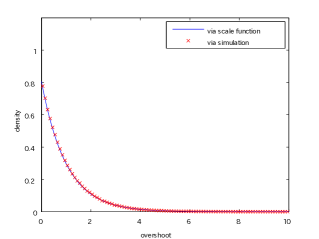
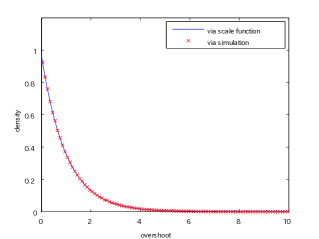
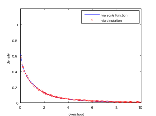
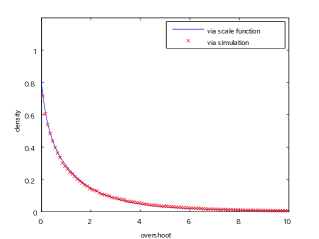
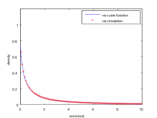
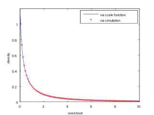
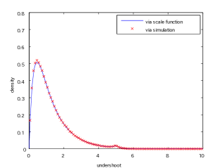
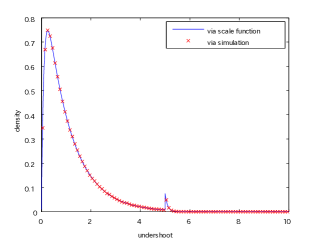
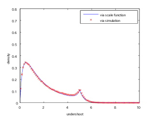
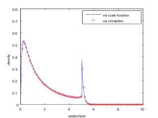
Figures 2 and 3 show the results for the cases and with common parameters , , and . From the results on the exponential case, we can confirm that the Monte Carlo simulated results are accurate. In Figure 3, the density has a jump at the initial position for the case (while it is continuous for the case ) due to the fact that is irregular for (see Definition 6.4 of [19]). As can be seen from these figures, the approximation accurately captures the overshoot/undershoot densities for and . The spike at the initial position in Figure 3 is precisely realized thanks to the closed-form expression (4.2); this would be difficult to realize if the scale function is approximated via numerical Laplace inversion.
 |
 |
| Exp(1) with | Exp(1) with |
 |
 |
| Weibull(0.6,0.665) with | Weibull(0.6,0.665) with |
 |
 |
| Pareto(1.2,5) with | Pareto(1.2,5) with |
 |
 |
| Exp(1) with | Exp(1) with |
 |
 |
| Weibull(0.6,0.665) with | Weibull(0.6,0.665) with |
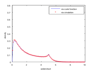 |
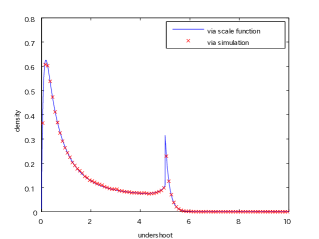 |
| Pareto(1.2,5) with | Pareto(1.2,5) with |
6 Concluding Remarks
In this paper, we studied and evaluated the performance of the phase-type fitting approach (motivated by [13]) for computing the Gerber-Shiu function for the spectrally negative Lévy process. The method is overall accurate and is powerful in that it can obtain an approximation in a closed form.
While this paper focused on the case of a spectrally negative Lévy process, the proposed method can easily be generalized. By the compensation formula, the decomposition (2.4) holds for a more general class of stochastic processes. Therefore, by simply replacing the resolvent measure , the Gerber-Shiu function can be computed in the same way.
Thanks to the recent developments of the fluctuation theories, the resolvents of various extensions of the spectrally negative Lévy process are now available in terms of the scale function. Here, we list several known examples of the resolvent.
-
1.
The fluctuation theories of reflected spectrally negative Lévy processes are well-developed. In the optimal dividend problem, where one wants to maximize the expected net present value of dividends until ruin, it is in many cases shown to be optimal to reflect the surplus process at a suitable boundary. It is therefore of interest to investigate the Gerber-Shiu function of the reflected process to evaluate the risk of an dividend paying company. As given in [31], the resolvent requires the derivative or the integral of the scale function, depending on whether the reflection barrier is upper or lower. For the doubly reflected case with both upper and lower barriers, see [30].
-
2.
As a variant of the reflected process, the refracted spectrally negative Lévy process of [21] changes its drift by whenever it is above a threshold – it is the unique strong solution to the stochastic differential equation
In insurance, this can be used to model the surplus of a dividend paying company when the dividend rate must be bounded from above by (see [22]). The resolvent is given in [21]. The resolvents for the cases with additional classical reflection have recently been obtained by [28, 29].
-
3.
Given two levels and , the classical -policy controls the process by pushing the process to immediately when it goes above or below . It is, under a suitable condition, an optimal strategy in the optimal dividend problem in the presence of a fixed cost (see [7, 25]). The resolvent is obtained in [35]. For its two-sided cases with four-parameter policy, see [34].
In these examples, the resolvent is written in terms of the scale function, and hence as in the cases considered in this paper, those for the phase-type case can be written as (a linear combination of) exponential forms. Consequently, the Gerber-Shiu function can be analytically computed in the same way. In view of the results obtained in this paper, the phase-type error is minimal and the same procedure is expected to give an accurate approximation of the Gerber-Shiu function.
References
- [1] H. Albrecher, F. Avram, and D. Kortschak: On the efficient evaluation of ruin probabilities for completely monotone claim distributions. Journal of Computational and Applied Mathematics, 233-10 (2010), 2724–2736.
- [2] S. Asmussen: Fitting phase-type distributions via the EM algorithm. Scandinavian Journal of Statistics, 23 (1996), 419-441.
- [3] S. Asmussen, F. Avram, and M.R. Pistorius: Russian and American put options under exponential phase-type Lévy models. Stochastic Processes and their Applications, 109-1 (2004), 79–111.
- [4] F. Avram, Z. Palmowski, and M.R. Pistorius: On the optimal dividend problem for a spectrally negative Lévy process. The Annals of Applied Probability, 17-1 (2007), 156–180.
- [5] O.E. Barndorff-Nielsen: Processes of normal inverse Gaussian type. Finance and Stochastics, 2-1 (1998), 41–68.
- [6] E. Bayraktar, A.E. Kyprianou, and K. Yamazaki: On optimal dividends in the dual model. Astin Bulletin, 43-3 (2013), 359–372.
- [7] E. Bayraktar, A.E. Kyprianou, and K. Yamazaki: Optimal dividends in the dual model under transaction costs. Insurance: Mathematics Economics, 54 (2014), 133–143.
- [8] S. Bernstein: Sur les fonctions absolument monotones. Acta Mathematica, 52-1 (1929), 1–66.
- [9] J. Bertoin: Lévy processes (Cambridge University Press, Cambridge, 1996).
- [10] P. Carr, H. Geman, D.B. Madan, and M. Yor: The structure of asset returns: an empirical investigation. Journal of Business, 75 (2002), 305–332.
- [11] T. Chan, A.E. Kyprianou, and M. Savov: Smoothness of scale functions for spectrally negative Lévy processes. Probability Theory and Related Fields, 150-3 (2011), 691–708.
- [12] E. Eberlein, U. Keller, and K. Prause: New insights into smile, mispricing and value at risk: the hyperbolic model. Journal of Business, 71 (1998), 371–405.
- [13] M. Egami and K. Yamazaki: Phase-type fitting of scale functions for spectrally negative Lévy processes. Journal of Computational and Applied Mathematics, 264 (2014), 1–22.
- [14] A. Feldmann and W. Whitt: Fitting mixtures of exponentials to long-tail distributions to analyze network performance models. Performance Evaluation, 31 (1998), 245-279.
- [15] J. Jacod and A.N. Shiryaev: Limit theorems for stochastic processes (Springer-Verlag, Berlin, 2003).
- [16] N. Johnson and S. Kotz: Distributions in statistics: continuous multivariate distributions (John Wiley & Sons Inc., New York, 1972)
- [17] D.W. Kammler: Chebyshev approximation of completely monotonic functions by sums of exponentials. SIAM Journal on Numerical Analysis, 13-5 (1976), 761–774.
- [18] A. Kuznetsov, A.E. Kyprianou, and V. Rivero: The theory of scale functions for spectrally negative Lévy processes. Lévy Matters II (Springer Lecture Notes in Mathematics), (Springer-Verlag, Berlin, 2013), 97-186.
- [19] A.E. Kyprianou: Fluctuations of Lévy processes with applications (second edition) (Springer-Verlag, Berlin, 2006).
- [20] A.E. Kyprianou: Gerber-Shiu Risk Theory (Springer-Verlag, Berlin, 2013).
- [21] A.E. Kyprianou and R. Loeffen: Refracted Lévy processes. Annales de l’Institut Henri Poincaré, Probabilités et Statistiques, 46-1 (2010), 24-44.
- [22] A.E. Kyprianou, R. Loeffen, and J.-L. Pérez: Optimal control with absolutely continuous strategies for spectrally negative Lévy processes. Journal of Applied Probability, 49-1 (2012), 150-166.
- [23] A.E. Kyprianou and B. Surya: Principles of smooth and continuous fit in the determination of endogenous bankruptcy levels. Finance and Stochastics, 11-1 (2007), 131–152.
- [24] R.L. Loeffen: On optimality of the barrier strategy in de Finetti’s dividend problem for spectrally negative Lévy processes. The Annals of Applied Probability, 18-5 (2008), 1669–1680.
- [25] R.L. Loeffen: An optimal dividends problem with transaction costs for spectrally negative Lévy processes. Insurance: Mathematics and Economics, 45-1 (2009), 41-48.
- [26] D.B. Madan, P. Carr, and E.C. Chang: The variance gamma processes and option pricing. European Finance Review, 2 (1998), 79–105.
- [27] D.B. Madan and F. Milne: Option pricing with VG martingale components. Mathematical Finance, 1-4 (1991), 39–55.
- [28] J.-L. Pérez and K. Yamazaki: On the refracted-reflected spectrally negative Lévy processes. arXiv:1511.06027, (2015).
- [29] J.-L. Pérez and K. Yamazaki: Refraction-reflection strategies in the dual model. Astin Bulletin, 47-1 (2017), 199-238.
- [30] M.R. Pistorius: On doubly reflected completely asymmetric Lévy process. Stochastic Processes and their Applications, 107-1 (2003), 131–143.
- [31] M.R. Pistorius: On exit and Ergodicity of the spectrally one-sided Lévy process reflected at its infimum. Journal of Theoretical Probability, 17-1 (2004), 183-220.
- [32] M.R. Pistorius: On maxima and ladder processes for a dense class of Lévy process. Journal of Applied Probability, 43-1 (2006), 208–220.
- [33] B. Surya: Evaluating scale functions of spectrally negative Lévy processes. Journal of Applied Probability, 45-1 (2008), 135–149.
- [34] K. Yamazaki: Cash management and control band policies for spectrally one-sided Lévy processes. Recent Advances in Financial Engineering 2014: Proceedings of the TMU Finance Workshop 2014 (World Scientific, 2016), 199-215.
- [35] K. Yamazaki: Inventory control for spectrally positive Lévy demand processes. Mathematics of Operations Research (forthcoming).
Kazutoshi Yamazaki
Department of Mathematics
Faculty of Engineering Science
Kansai University
3-3-35 Yamate-cho, Suita-shi,
Osaka 564-8680, Japan
E-mail: kyamazak@kansai-u.ac.jp