Empirical spectral distribution of a matrix under perturbation

Abstract.

We provide a perturbative expansion for the empirical spectral distribution of a Hermitian matrix with large size perturbed by a random matrix with small operator norm whose entries in the eigenvector basis of the first one are independent with a variance profile. We prove that, depending on the order of magnitude of the perturbation, several regimes can appear, called perturbative and semi-perturbative regimes. Depending on the regime, the leading terms of the expansion are either related to the one-dimensional Gaussian free field or to free probability theory.

1. Introduction

It is a natural and central question, in mathematics and physics, to understand how the spectral properties of an operator are altered when the operator is subject to a small perturbation. This question is at the center of Perturbation Theory and has been studied in many different contexts. We refer the reader to Kato’s book [17] for a thorough account on this subject. In this text, we provide a perturbative expansion for the empirical spectral distribution of a Hermitian matrix with large size perturbed by a random matrix with small operator norm whose entries in the eigenvector basis of the first one are independent with a variance profile. More explicitly, let $D_{n}$ be an $n\times n$ Hermitian matrix, that, up to a change of basis, we suppose diagonal. We denote by $\mu_{n}$ the empirical spectral distribution of $D_{n}$. This matrix is additively perturbed by a random Hermitian matrix $\varepsilon_{n}X_{n}$ whose entries are chosen at random independently and scaled so that the operator norm of $X_{n}$ has order one. We are interested in the empirical spectral distribution $\mu_{n}^{\varepsilon}$ of

$$D_{n}^{\varepsilon}\;:=\;D_{n}+\varepsilon_{n}X_{n}$$

in the regime where the matrix size $n$ tends to infinity and $\varepsilon_{n}$ tends to $0$. We shall prove that, depending on the order of magnitude of the perturbation, several regimes can appear. We suppose that $\mu_{n}$ converges to a limiting measure $\rho(\lambda)\mathrm{d}\lambda$ and that the variance profile of the entries of $X_{n}$ has a macroscopic limit $\sigma_{\operatorname{d}}$ on the diagonal and $\sigma$ elsewhere. We then prove that there is a deterministic function $F$ and a Gaussian random linear form $\mathrm{d}Z$ on the space of $\mathcal{C}^{6}$ functions on $\mathbb{R}$, both depending only on the limit parameters of the model $\rho,\sigma$ and $\sigma_{\operatorname{d}}$ such that if one defines the distribution $\mathrm{d}F:\phi\longmapsto-\int\phi^{\prime}(s)F(s)\mathrm{d}s$, then, for large $n$:

$$\hskip 128.0374pt\mu_{n}^{\varepsilon} \;\approx\;\mu_{n}+\frac{\varepsilon_{n}}{n}\mathrm{d}Z \varepsilon_{n}\ll n^{-1}$$ if (1)

$$\qquad\mu_{n}^{\varepsilon} \;\approx\;\mu_{n}+\frac{\varepsilon_{n}}{n}\left(c\mathrm{d}F+\mathrm{d}Z\right) \varepsilon_{n}\sim\frac{c}{n}$$ if (2)

$$\qquad\mu_{n}^{\varepsilon} \;\approx\;\mu_{n}+\varepsilon_{n}^{2}\mathrm{d}F n^{-1}\ll\varepsilon_{n}\ll 1$$ if (3)

and if, moreover, $n^{-1}\ll\varepsilon_{n}\ll n^{-1/3},$ then convergence (3) can be refined as follows:

$$\;\mu_{n}^{\varepsilon} \;\approx\;\mu_{n}+\varepsilon_{n}^{2}\mathrm{d}F+\frac{\varepsilon_{n}}{n}\mathrm{d}Z.$$ (4)

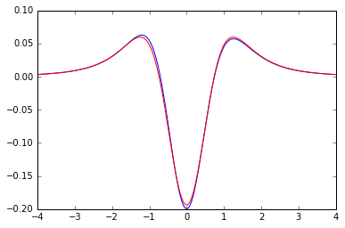
In Section 3 several figures show a very good matching of random simulations with these theoretical results. The definitions of the function $F$ and of the process $Z$ are given below in (6) and (7). In many cases, the linear form $\mathrm{d}F$ can be interpreted as the integration with respect to the signed measure $F^{\prime}(x)\mathrm{d}x$. The function $F$ is related to free probability theory, as explained in Section 4 below, whereas the linear form $\mathrm{d}Z$ is related to the so-called one-dimensional Gaussian free field defined, for instance, at [14, Sect. 4.2]. If the variance profile of $X_{n}$ is constant, then it is precisely the Laplacian of the Gaussian free field, defined in the sense of distributions.

The transition at $\varepsilon_{n}\sim n^{-1}$ is the well-known transition, in quantum mechanics, where the perturbative regime ends. Indeed, one can distinguish the two following regimes:

• The regime $\varepsilon_{n}\ll n^{-1}$, called the perturbative regime (see [15]): the size of the perturbation (i.e. its operator norm) is much smaller than the typical spacing between two consecutive eigenvalues (level spacing), which is of order $n^{-1}$ in our setting.
  

• The regime $n^{-1}\ll\varepsilon_{n}\ll 1$, sometimes called the semi-perturbative regime, where the size of the perturbation is not small compared to the level spacing. This regime concerns many applications [19, 1] in the context of covariance matrices and applications to finance.

A surprising fact discovered during this study is that the semi-perturbative regime $n^{-1}\ll\varepsilon_{n}\ll 1$ decomposes into infinitely many sub-regimes. In the case $n^{-1}\ll\varepsilon_{n}\ll n^{-1/3}$, the expansion of $\mu_{n}^{\varepsilon}-\mu_{n}$ contains a single deterministic term before the random term $\frac{\varepsilon_{n}}{n}\mathrm{d}Z$. In the case $n^{-1/3}\ll\varepsilon_{n}\ll n^{-1/5}$, the expansion of $\mu_{n}^{\varepsilon}-\mu_{n}$ contains two of them. More generally, for all positive integer $p$, when $n^{-1/(2p-1)}\ll\varepsilon_{n}\ll n^{-1/(2p+1)}$, the expansion contains $p$ of them. For computational complexity reasons, the only case we state explicitly is the first one. We refer the reader to Section 6.5 for a discussion around this point.

In the papers [23, 1, 2, 4, 3], Wilkinson, Walker, Allez, Bouchaud et al have investigated some problems related to this one. Some of these works were motivated by the estimation of a matrix out of the observation of its noisy version. Our paper differs from these ones mainly by the facts that firstly, we are interested in the perturbations of the global empirical distribution of the eigenvalues and not of a single one, and secondly, we push our expansion up to the random term, which does not appear in these papers. Besides, the noises they consider have constant variance profiles (either a Wigner-Dyson noise in the four first cited papers or a rotationally invariant noise in the fifth one). The transition at $\varepsilon_{n}\sim n^{-1}$ between the perturbative and the semi-perturbative regimes is already present in these texts. They also consider the transition between the perturbative regime $\varepsilon_{n}\ll 1$ and the non perturbative regime $\varepsilon_{n}\asymp 1$. As explained above, we exhibit the existence of an infinity of sub-regimes in this transition and focus on $\varepsilon_{n}\ll 1$ for the first order of the expansion and to $\varepsilon_{n}\ll n^{-1/3}$ for the second (and last) order. The study of other sub-regimes is postponed to forthcoming papers.

The paper is organized as follows. Results, examples and comments are given in Sections 2 to 4, while the rest of the paper, including an appendix, is devoted to the proofs, except for Section 6.5, where we discuss the sub-regimes mentioned above.

Notations. For $a_{n},b_{n}$ some real sequences, $a_{n}\ll b_{n}$ (resp. $a_{n}\sim b_{n}$) means that $a_{n}/b_{n}$ tends to $0$ (resp. to $1$). Also, $\stackrel{{\scriptstyle P}}{{\longrightarrow}}$ and $\stackrel{{\scriptstyle\mathrm{dist.}}}{{\longrightarrow}}$ stand respectively for convergence in probability and convergence in distribution for all finite marginals.

2. Main result

2.1. Definition of the model and assumptions

For all positive integer $n$, we consider a real diagonal matrix $D_{n}=\operatorname{diag}(\lambda_{n}(1),\ldots,\lambda_{n}(n))$, as well as a Hermitian random matrix

$$X_{n}=\frac{1}{\sqrt{n}}[x^{n}_{i,j}]_{1\leq i,j\leq n}$$

and a positive number $\varepsilon_{n}$. The normalizing factor $n^{-1/2}$ and our hypotheses below ensure that the operator norm of $X_{n}$ is of order one. We then define, for all $n$,

$$D_{n}^{\varepsilon}:=D_{n}+\varepsilon_{n}X_{n}.$$

We now introduce the probability measures $\mu_{n}$ and $\mu_{n}^{\varepsilon}$ as the respective uniform distributions on the eigenvalues (with multiplicity) of $D_{n}$ and $D_{n}^{\varepsilon}$. Our aim is to give a perturbative expansion of $\mu_{n}^{\varepsilon}$ around $\mu_{n}$.

We make the following hypotheses:

1. the entries $x^{n}_{i,j}$ of $\sqrt{n}X_{n}$ are independent (up to symmetry) random variables, centered, with variance denoted by $\sigma_{n}^{2}(i,j)$, such that $\mathbb{E}|x^{n}_{i,j}|^{8}$ is bounded uniformly on $n,i,j$,
   

2. there are $f,\sigma_{\operatorname{d}},\sigma$ real functions defined respectively on $[0,1]$, $[0,1]$ and $[0,1]^{2}$ such that, for each $x\in[0,1]$,

   $$\lambda_{n}(\lfloor nx\rfloor)\underset{n\to\infty}{\longrightarrow}f(x)\quad\textrm{ and }\quad\sigma_{n}^{2}(\lfloor nx\rfloor,\lfloor nx\rfloor)\underset{n\to\infty}{\longrightarrow}\sigma_{\operatorname{d}}(x)^{2}$$

   and for each $x\neq y\in[0,1]$,

   $$\sigma_{n}^{2}(\lfloor nx\rfloor,\lfloor ny\rfloor)\underset{n\to\infty}{\longrightarrow}\sigma^{2}(x,y).$$

   We make the following hypothesis about the rate of convergence:

   $$\eta_{n}\;:=\;\max\{n\varepsilon_{n},1\}\times\sup_{1\leq i\neq j\leq n}(|\sigma_{n}^{2}(i,j)-\sigma^{2}(i/n,j/n)|+|\lambda_{n}(i)-f(i/n)|)\quad\underset{n\to\infty}{\longrightarrow}\quad 0.$$

Let us now make some assumptions on the limiting functions $\sigma$ and $f$:

1. the function $f$ is bounded and the push-forward of the uniform measure on $[0,1]$ by the function $f$ has a density $\rho$ with respect to the Lebesgue measure on $\mathbb{R}$ and a compact support denoted by $\mathcal{S}$,
   

2. the variance of the entries of $X_{n}$ essentially depends on the eigenspaces of $D_{n}$, namely, there exists a symmetric function $\tau(\,\cdot\,,\,\cdot\,)$ on $\mathbb{R}^{2}$ such that for all $x\neq y$, $\sigma^{2}(x,y)=\tau(f(x),f(y))$,
   

3. the following regularity property holds: there exist $\eta_{0}>0,\alpha>0$ and $C<\infty$ such that for almost all $s\in\mathbb{R}$, for all $t\in[s-\eta_{0},s+\eta_{0}]$, $|\tau(s,t)\rho(t)-\tau(s,s)\rho(s)|\leq C|t-s|^{\alpha}$.

We add a last assumption which strengthens assumption (c) and makes it possible to include the case where the set of eigenvalues of $D_{n}$ contains some outliers:

1. there is a real compact set $\widetilde{\mathcal{S}}$ such that

   $$\max_{1\leq i\leq n}\operatorname{dist}(\lambda_{n}(i),\widetilde{\mathcal{S}})\underset{n\to\infty}{\longrightarrow}0.$$

Remark 1 (About the hypothesis that $D_{n}$ is diagonal).

(i) If the perturbing matrix $X_{n}$ belongs to the GOE (resp. to the GUE), then its law is invariant under conjugation by any orthogonal (resp. unitary) matrix. It follows that in this case, our results apply to any real symmetric (resp. Hermitian) matrix $D_{n}$ with eigenvalues $\lambda_{n}(i)$ satisfying the above hypotheses.

(ii) As explained after Proposition 2 below, we conjecture that when the variance profile of $X_{n}$ is constant, for $\varepsilon_{n}\gg n^{-1}$, we do not need the hypothesis that $D_{n}$ is diagonal neither. However, if the perturbing matrix does not have a constant variance profile, then for a non-diagonal $D_{n}$ and $\varepsilon\gg n^{-1}$, the spectrum of $D_{n}^{\varepsilon}$ should depend heavily on the relation between the eigenvectors of $D_{n}$ and the variance profile, which implies that our results should not remain true.

(iii) At last, it is easy to see that the random process $(Z_{\phi})$ introduced at (7) satisfies, for any test function $\phi$,

$$\frac{1}{\varepsilon_{n}}\sum_{i=1}^{n}\left(\phi(\lambda_{n}(i)+\frac{\varepsilon_{n}}{\sqrt{n}}x_{ii})-\phi(\lambda_{n}(i))\right)\quad\stackrel{{\scriptstyle\mathrm{dist.}}}{{\underset{n\to\infty}{\longrightarrow}}}\quad Z_{\phi}.$$

Thus, regardless to the variance profile, the convergence of (8) rewrites, informally,

$$\mu_{n}^{\varepsilon}=\frac{1}{n}\sum_{i=1}^{n}\delta_{\lambda_{n}(i)+(\varepsilon_{n}/\sqrt{n})x_{ii}}+o(\varepsilon_{n}/n).$$ (5)

A so simple expression, up to a $o(\varepsilon_{n}/n)$ error, of the empirical spectral distribution of $D_{n}^{\varepsilon}$, with some independent translations $\frac{\varepsilon}{\sqrt{n}}x_{ii}$, should not remain true without the hypothesis that $D_{n}$ is diagonal or that the distribution of $X_{n}$ is invariant under conjugation.

2.2. Main result

Recall that the Hilbert transform, denoted by $H[u]$, of a function $u$, is the function

$$H[u](s):=\operatorname{p.v.}\int_{t\in\mathbb{R}}\frac{u(t)}{s-t}\mathrm{d}t$$

and define the function

$$F(s)=-\rho(s)H[\tau(s,\cdot)\rho(\cdot)](s).$$ (6)

Note that, by assumptions (c) and (e), $F$ is well defined and supported by $\mathcal{S}$. Besides, for any $\phi$ supported on an interval where $F$ is $\mathcal{C}^{1}$,

$$-\int\phi^{\prime}(s)F(s)\mathrm{d}s=\int\phi(s)\mathrm{d}F(s),$$

where $\mathrm{d}F(s)$ denotes the measure $F^{\prime}(s)\mathrm{d}s$.

We also introduce the centered Gaussian field, $(Z_{\phi})_{\phi\in\mathcal{C}^{6}}$, indexed by the set of $\mathcal{C}^{6}$ complex functions on $\mathbb{R}$, with covariance defined by

$$\mathbb{E}Z_{\phi}Z_{\psi}\;=\;\int_{0}^{1}\sigma_{\operatorname{d}}(t)^{2}\phi^{\prime}(f(t))\psi^{\prime}(f(t))\mathrm{d}t\qquad\textrm{ and }\qquad\overline{Z_{\psi}}\;=\;Z_{\overline{\psi}}.$$ (7)

Note that the process $(Z_{\phi})_{\phi\in\mathcal{C}^{6}}$ can be represented, for $(B_{t})$ is the standard one-dimensional Brownian motion, as

$$Z_{\phi}=\int_{0}^{1}\sigma_{\operatorname{d}}(t)\phi^{\prime}(f(t))\mathrm{d}B_{t}.$$

Theorem 1.

For all compactly supported $\mathcal{C}^{6}$ function $\phi$ on $\mathbb{R}$, the following convergences hold:

$\bullet$ Perturbative regime: if $\varepsilon_{n}\ll n^{-1}$, then,

$$n\varepsilon_{n}^{-1}(\mu_{n}^{\varepsilon}-\mu_{n})(\phi)\quad\stackrel{{\scriptstyle\mathrm{dist.}}}{{\underset{n\to\infty}{\longrightarrow}}}\quad Z_{\phi}.$$ (8)

$\bullet$ Critical regime: if $\varepsilon_{n}\sim c/n$, with $c$ constant, then,

$$n\varepsilon_{n}^{-1}(\mu_{n}^{\varepsilon}-\mu_{n})(\phi)\quad\stackrel{{\scriptstyle\mathrm{dist.}}}{{\underset{n\to\infty}{\longrightarrow}}}\quad-c\int\phi^{\prime}(s)F(s)\mathrm{d}s+Z_{\phi}.$$ (9)

$\bullet$ Semi-perturbative regime: if $n^{-1}\ll\varepsilon_{n}\ll 1$, then,

$$\varepsilon_{n}^{-2}(\mu_{n}^{\varepsilon}-\mu_{n})(\phi)\quad\stackrel{{\scriptstyle P}}{{\underset{n\to\infty}{\longrightarrow}}}\quad-\int\phi^{\prime}(s)F(s)\mathrm{d}s,$$ (10)

and if, moreover, $n^{-1}\ll\varepsilon_{n}\ll n^{-1/3}$, then,

$$n\varepsilon_{n}^{-1}\left((\mu_{n}^{\varepsilon}-\mu_{n})(\phi)+\varepsilon_{n}^{2}\int\phi^{\prime}(s)F(s)\mathrm{d}s\right)\quad\stackrel{{\scriptstyle\mathrm{dist.}}}{{\underset{n\to\infty}{\longrightarrow}}}\quad Z_{\phi}.$$ (11)

Remark 2 (Sub-regimes for $n^{-1/3}\ll\varepsilon_{n}\ll 1$).

In the semi-perturbative regime, the reason why we provide an expansion up to a random term, only for $\varepsilon_{n}\ll n^{-1/3}$, is that the study of the regime $n^{-1/3}\ll\varepsilon_{n}\ll 1$ up to such a precision, requires further terms in the expansion of the resolvent of $D_{n}^{\varepsilon}$ that make appear, beside $\mathrm{d}F$, additional determistic terms of smaller order, which are much larger than the probabilistic term containing $Z_{\phi}$. The computation becomes rather intricate without any clear recursive formula. As we will see in Section 6.5, there are infinitely many regimes. Precisely, for any positive integer $p$, when $n^{-1/(2p-1)}\ll\varepsilon_{n}\ll n^{-1/(2p+1)}$, there are $p$ deterministic terms in the expansion before the term in $Z_{\phi}$.

Remark 3 (Local law).

The approximation

$$\mu_{n}^{\varepsilon}(I)\;\approx\;\mu_{n}(I)+\varepsilon_{n}^{2}\int_{I}\mathrm{d}F$$

of (10) should stay true even for intervals $I$ with size tending to $0$ as the dimension $n$ grows, as long as the size of $I$ stays much larger than the right-hand side term of (30), as can be seen from Proposition 5.

Remark 4.

The second part of Hypothesis (b), concerning the speed of convergence of the profile of the spectrum of $D_{n}$ as well as of the variance of its perturbation, is needed in order to express the expansion of $\mu_{n}^{\varepsilon}-\mu_{n}$ in terms of limit parameters of the model $\sigma$ and $\rho$. We can remove this hypothesis and get analogous expansions where the terms $\mathrm{d}F$ and $\mathrm{d}Z$ are replaced by their discrete counterparts $\mathrm{d}F_{n}$ and $\mathrm{d}Z_{n}$, defined thanks to the “finite $n$” empirical versions of the limit parameters $\sigma$ and $\rho$.

3. Examples

3.1. Uniform measure perturbation by a band matrix

Here, we consider the case where $f(x)=x$, $\sigma_{\operatorname{d}}(x)\equiv m$ and $\sigma(x,y)=\mathbbm{1}_{|y-x|\leq\ell}$, for some constants $m\geq 0$ and $\ell\in[0,1]$ (the relative width of the band). In this case, $\tau(\,\cdot\,,\,\cdot\,)=\sigma(\,\cdot\,,\,\cdot\,)^{2}$, hence

$$F(s)\;=\;\mathbbm{1}_{(0,1)}(s)\operatorname{p.v.}\int_{t}\frac{\tau(s,t)}{s-t}\mathrm{d}t\;=\;-\mathbbm{1}_{(0,1)}(s)\log\frac{\ell\wedge(1-s)}{\ell\wedge s}$$ (12)

and $(Z_{\phi})_{\phi\in\mathcal{C}^{6}}$ is the centered complex Gaussian process with covariance defined by

$$\mathbb{E}Z_{\phi}\overline{Z_{\psi}}\;=\;m^{2}\int_{0}^{1}\phi^{\prime}(t)\ \overline{\psi^{\prime}(t)}\ \mathrm{d}t\qquad\textrm{ and }\qquad\overline{Z_{\psi}}\;=\;Z_{\overline{\psi}}.$$

Theorem 1 is then illustrated by Figure 1, where we ploted the cumulative distribution functions.

(a) $n=10^{4}$, $\varepsilon_{n}=n^{-0.4}$, $\ell=0.2$

(b) $n=10^{4}$, $\varepsilon_{n}=n^{-0.4}$, $\ell=0.8$

Figure 1. Deforming the uniform distribution by a band matrix. Cumulative distribution function of $\varepsilon_{n}^{-2}(\mu_{n}^{\varepsilon}-\mu_{n})$ (in blue) and function $F(\,\cdot\,)$ of (12) (in red). The non smoothness of the blue curves results of the noise term $Z_{\phi}$ in Theorem 1. Each graphic is realized thanks to one single matrix (no averaging) perturbed by a real Gaussian band matrix.

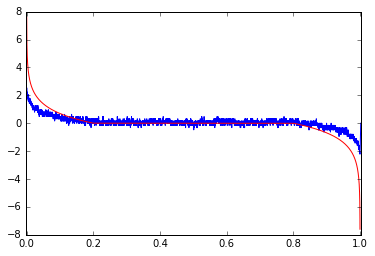
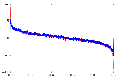
3.2. Triangular pulse perturbation by a Wigner matrix

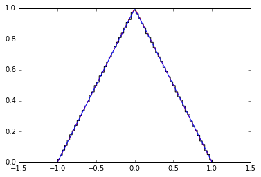
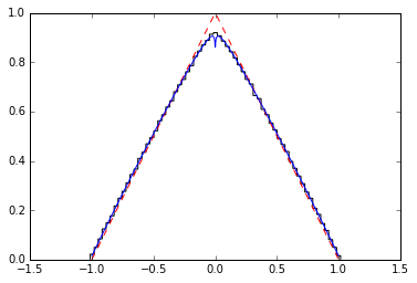
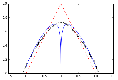
Here, we consider the case where $\rho(x)=(1-|x|)\mathbbm{1}_{[-1,1]}(x)$, $\sigma_{d}\equiv m$, for some real constant $m$, and $\sigma\equiv 1$ (what follows can be adapted to the case $\sigma(x,y)=\mathbbm{1}_{|y-x|\leq\ell}$, with a bit longer formulas). In this case, thanks to the formula (9.6) of $H[\rho(\,\cdot\,)]$ given p. 509 of [18], we get

$$F(s)\;=\;(1-|s|)\mathbbm{1}_{[-1,1]}(s)\left\{(1-s)\log(1-s)-(1+s)\log(1+s)+2s\log|s|\right\}.$$ (13)

and the covariance of $(Z_{\phi})_{\phi\in\mathcal{C}^{6}}$ is given by

$$\mathbb{E}Z_{\phi}\overline{Z_{\psi}}\;=\;m^{2}\int_{-1}^{1}(1-|t|)\ \phi^{\prime}(t)\ \overline{\psi^{\prime}(t)}\ \mathrm{d}t\qquad\textrm{ and }\qquad\overline{Z_{\psi}}\;=\;Z_{\overline{\psi}}.$$

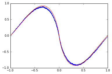
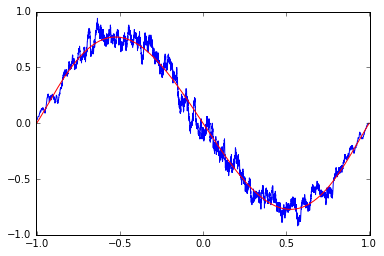
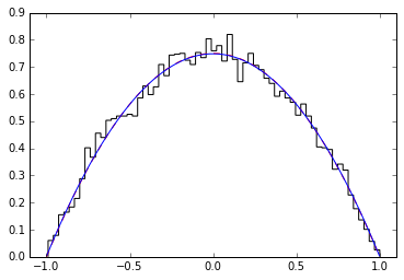
Theorem 1 is then illustrated by Figure 2 in the case where $\varepsilon_{n}\gg n^{-1/2}$. In Figure 2, we implicitly use some test functions of the type $\phi(x)=\mathbbm{1}_{x\in I}$ for some intervals $I$. These functions are not $\mathcal{C}^{6}$, and one can easily see that for $\varepsilon_{n}\ll n^{-1/2}$, Theorem 1 cannot work for such functions. However, considering imaginary parts of Stietljes transforms, i.e. test functions

$$\phi(x)=\frac{1}{\pi}\frac{\eta}{(x-E)^{2}+\eta^{2}}\qquad(E\in\mathbb{R},\;\eta>0)$$

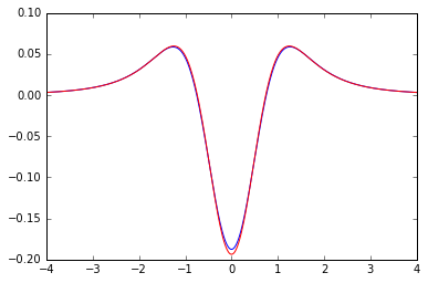
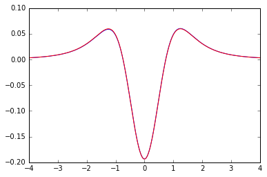
gives a perfect matching between the predictions from Theorem 1 and numerical simulations, also for $\varepsilon_{n}\ll n^{-1/2}$ (see Figure 3, where we use Proposition 4 and (17) to compute the theoretical limit).

Figure 2. Triangular pulse perturbation by a Wigner matrix: density and cumulative distribution function. Top left: Cumulative distribution function of $\varepsilon_{n}^{-2}(\mu_{n}^{\varepsilon}-\mu_{n})$(in blue) and function $F(\,\cdot\,)$ of (13) (in red). Top right and bottom: Density $\rho$ (red dashed line), histogram of the eigenvalues of $D_{n}^{\varepsilon}$ (in black) and theoretical density $\rho+\varepsilon_{n}^{2}F^{\prime}(s)$ of the eigenvalues of $D_{n}^{\varepsilon}$ as predicted by Theorem 1 (in blue). Here, $n=10^{4}$ and $\varepsilon_{n}=n^{-\alpha}$, with $\alpha=0.25$ (up left), $\alpha=0.4$ (up right), $0.25$ (bottom left) and $0.1$ (bottom right).

Figure 3. Triangular pulse perturbation by a Wigner matrix: Stieltjes transform. Imaginary part of the Stieltjes transform of $\varepsilon_{n}^{-2}(\mu_{n}^{\varepsilon}-\mu_{n})$ (in blue) and of the measure $\mathrm{d}F$ (in red) at $z=E+\mathrm{i}$ as a function of the real part $E$ for different values of $\varepsilon_{n}$. Here, $n=10^{4}$ and $\varepsilon_{n}=n^{-\alpha}$, with $\alpha=0.2$, $0.5$ and $0.8$ (from left to right).

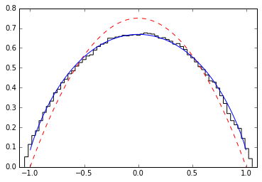
3.3. Parabolic pulse perturbation by a Wigner matrix

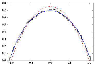
Here, we consider the case where $\rho(x)=\frac{3}{4}(1-x^{2})\mathbbm{1}_{[-1,1]}(x)$, $\sigma_{d}\equiv m$, for some real constant $m$, and $\sigma\equiv 1$ (again, this can be adapted to the case $\sigma(x,y)=\mathbbm{1}_{|y-x|\leq\ell}$). Theorem 1 is then illustrated by Figure 4. In this case, thanks to the formula (9.10) of $H[\rho(\,\cdot\,)]$ given p. 509 of [18], we get

$$F(s)\;=\;-\frac{9}{16}(1-s^{2})\mathbbm{1}_{[-1,1]}(s)\left\{2s-(1-s^{2})\ln\left|\frac{s-1}{s+1}\right|\right\}$$ (14)

and the covariance of $(Z_{\phi})_{\phi\in\mathcal{C}^{6}}$ is given by

$$\mathbb{E}Z_{\phi}\overline{Z_{\psi}}\;=\;\frac{3m^{2}}{4}\int_{-1}^{1}(1-t^{2})\ \phi^{\prime}(t)\ \overline{\psi^{\prime}(t)}\ \mathrm{d}t\qquad\textrm{ and }\qquad\overline{Z_{\psi}}\;=\;Z_{\overline{\psi}}.$$

Figure 4. Parabolic pulse perturbation by a Wigner matrix. Top left: Cumulative distribution function of $\varepsilon_{n}^{-2}(\mu_{n}^{\varepsilon}-\mu_{n})$(in blue) and function $F(\,\cdot\,)$ of (14) (in red). Top right and bottom: Density $\rho$ (red dashed line), histogram of the eigenvalues of $D_{n}^{\varepsilon}$ (in black) and theoretical density $\rho+\varepsilon_{n}^{2}F^{\prime}(s)$ of the eigenvalues of $D_{n}^{\varepsilon}$ as predicted by Theorem 1 (in blue). Here, $n=10^{4}$ and $\varepsilon_{n}=n^{-\alpha}$, with $\alpha=0.25$ (up left), $\alpha=0.4$ (up right), $0.2$ (bottom left) and $0.18$ (bottom right).

4. Relation to free probability theory

Let us now explain how this work is related to free probability theory. If, instead of letting $\varepsilon_{n}$ tend to zero, one considers the model

$$D_{n}^{t}\;:=\;D_{n}+\sqrt{t}X_{n}$$

for a fixed $t>0$, then, by [12, 13, 22, 5], the empirical eigenvalue distribution of $D_{n}^{t}$ has a limit as $n\to\infty$, that we shall denote here by $\mu_{t}$. The law $\mu_{t}$ can be interpreted as the law of the sum of two elements in a non-commutative probability space which are free with an amalgamation over a certain sub-algebra (see [22] for more details). The following proposition relates the function $F$ from (6) to the first order expansion of $\mu_{t}$ around $t=0$.

Proposition 2.

For any $z\in\mathbb{C}\backslash\mathbb{R}$, we have

$$\frac{\partial}{\partial t}_{|t=0}\int\frac{\mathrm{d}\mu_{t}(\lambda)}{z-\lambda}\;=\;-\int\frac{F(\lambda)}{(z-\lambda)^{2}}\mathrm{d}\lambda\;=\;-\int F(\lambda)\frac{\partial}{\partial\lambda}\left(\frac{1}{z-\lambda}\right)\mathrm{d}\lambda.$$

This is related to the fact that in Equations (1)–(4), for $\varepsilon_{n}$ large enough, the term $\varepsilon_{n}^{2}\mathrm{d}F$ is the leading term.

In the particular case where $X_{n}$ is a Wigner matrix, $\mu_{t}$ is the free convolution of the measure $\rho(\lambda)\mathrm{d}\lambda$ with a semicircle distribution and admits a density $\rho_{t}$, by [8, Cor. 2]. Then, Theorem 1 makes it possible to formally recover the free Fokker-Planck equation with null potential:

$$\begin{cases}\frac{\partial}{\partial t}\rho_{t}(s)+\frac{\partial}{\partial s}\{\rho_{t}(s)H[\rho_{t}](s)\}=0,\\ \rho_{0}(s)=\rho(s),\end{cases}$$

where $H[\rho_{t}]$ denotes the Hilbert transform of $\rho_{t}$. This equation is also called McKean-Vlasov (or Fokker-Planck) equation with logarithmic interaction (see [9, 10, 11]).

Note also that when $X_{n}$ is a Wigner matrix, the hypothesis that $D_{n}$ is diagonal is not required to have the convergence of the empirical eigenvalue distribution of $D_{n}^{t}$ to $\mu_{t}$ as $n\to\infty$. This suggests that, even for non diagonal $D_{n}$, the convergence of (10) still holds when $X_{n}$ is a Wigner matrix.

Proof of Proposition 2. By [22, Th. 4.3], we have

$$\int\frac{\mathrm{d}\mu_{t}(\lambda)}{z-\lambda}\;=\;\int_{x=0}^{1}C_{t}(x,z)\mathrm{d}x,$$ (15)

where $C_{t}(x,z)$ is bounded by $|\mathfrak{Im}z|^{-1}$ and satisfies the fixed-point equation

$$C_{t}(x,z)=\frac{1}{z-f(x)-t\int_{y=0}^{1}\sigma^{2}(x,y)C_{t}(y,z)\mathrm{d}y}.$$

Hence as $t\to 0$, $C_{t}(x,z)\longrightarrow\frac{1}{z-f(x)}$ uniformly in $x$. Thus

$$C_{t}(x,z)-\frac{1}{z-f(x)} = \frac{t\int_{y=0}^{1}\sigma^{2}(x,y)C_{t}(y,z)\mathrm{d}y}{(z-f(x)-t\int_{y=0}^{1}\sigma^{2}(x,y)C_{t}(y,z)\mathrm{d}y)(z-f(x))}$$

$$= t\frac{1}{(z-f(x))^{2}}\int_{y=0}^{1}\sigma^{2}(x,y)C_{t}(y,z)\mathrm{d}y+o(t)$$

$$= t\frac{1}{(z-f(x))^{2}}\int_{y=0}^{1}\frac{\sigma^{2}(x,y)}{z-f(y)}\mathrm{d}y+o(t)$$

where each $o(t)$ is uniform in $x\in[0,1]$. Then, by (15), we deduce that

$$\frac{\partial}{\partial t}_{|t=0}\int\frac{\mathrm{d}\mu_{t}(\lambda)}{z-\lambda}=\int_{(x,y)\in[0,1]^{2}}\frac{\sigma^{2}(x,y)}{(z-f(x))^{2}(z-f(y))}\mathrm{d}x\mathrm{d}y.$$

The right-hand side term of the previous equation is precisely the number $B(z)$ introduced at (17) below. Then, one concludes using Proposition 4 from Section 6.1. $\square$

5. Strategy of the proof

We shall first prove the convergence results of Theorem 1 for test functions $\phi$ of the form $\varphi_{z}(x):=\frac{1}{z-x}$. This is done in Section 6 by writing an expansion of the resolvent of $D_{n}^{\varepsilon}$.

Once we have proved that the convergences hold for the resolvent of $D_{n}^{\varepsilon}$, we can extend them to the larger class of compactly supported $\mathcal{C}^{6}$ functions on $\mathbb{R}$.

In Section 7, we use the Helffer-Sjöstrand formula to extend the convergence in probability in the semi-pertubative regime (10) to the case of compactly supported $\mathcal{C}^{6}$ functions on $\mathbb{R}$.

In Section 8, the convergences in distribution (8), (9) and (11) are proved in two steps. The overall strategy is to apply an extension lemma of Shcherbina and Tirozzi which states that a CLT that applies to a sequence of centered random linear forms on some space can be extended, by density, to a larger space, as long as the variance of the image of these random linear forms by a function $\phi$ of the larger space is uniformly bounded by the norm of $\phi$. Therefore, our task is twofold. We need first to prove that the sequences of variables involved in the convergences (8), (9) and (11) can be replaced by their centered counterparts $n\varepsilon_{n}^{-1}(\mu_{n}^{\varepsilon}(\phi)-\mathbb{E}[\mu_{n}^{\varepsilon}(\phi)])$ (i.e. they differ by $o(1)$). In a second step, we dominate the variance of these latter variables, in order to apply the extension lemma which is precisely stated in the appendix as Lemma 10.

6. Stieltjes transforms convergence

As announced in the previous section, we start with the proof of Theorem 1 in the special case of test functions of the type $\varphi_{z}:=\frac{1}{z-x}$. We decompose it into two propositions. Their statement and proof are the purpose of the three following subsections. The two last subsections 6.4 and 6.5 are devoted respectively to a local type convergence result and to a discussion about the possibility of an extension of the expansion result to a wider range of rate of convergence of $\varepsilon_{n}$, namely beyond $n^{-1/3}$.

6.1. Two statements

Let denote, for $z\in\mathbb{C}\backslash\mathbb{R}$,

$$Z(z):=Z_{\varphi_{z}}\quad\textrm{ for }\quad\varphi_{z}(x):=\frac{1}{z-x}$$ (16)

where $(Z_{\phi})_{\phi\in\mathcal{C}^{6}}$ is the Gaussian field with covariance defined by (7). We also introduce, for $z\in\mathbb{C}\backslash\mathbb{R}$,

$$B(z):=\int_{(s,t)\in[0,1]^{2}}\frac{\sigma^{2}(s,t)}{(z-f(s))^{2}(z-f(t))}\mathrm{d}s\mathrm{d}t$$ (17)

and

$$\Delta\mathrm{G}_{n}(z)\;:=\;(\mu_{n}^{\varepsilon}-\mu_{n})(\varphi_{z})\;=\;\frac{1}{n}\operatorname{Tr}\frac{1}{z-D_{n}^{\varepsilon}}-\frac{1}{n}\operatorname{Tr}\frac{1}{z-D_{n}}.$$ (18)

Proposition 3.

Under Hypotheses (a), (b), (f),

• if $\varepsilon_{n}\ll n^{-1}$, then for all $z\in\mathbb{C}\backslash\mathbb{R}$,

  $$n\varepsilon_{n}^{-1}\Delta\mathrm{G}_{n}(z)\quad\stackrel{{\scriptstyle\mathrm{dist.}}}{{\underset{n\to\infty}{\longrightarrow}}}\quad Z(z)\,$$ (19)

• if $\varepsilon_{n}\sim c/n$, with $c$ constant, then for all $z\in\mathbb{C}\backslash\mathbb{R}$

  $$n\varepsilon_{n}^{-1}\Delta\mathrm{G}_{n}(z)\quad\stackrel{{\scriptstyle\mathrm{dist.}}}{{\underset{n\to\infty}{\longrightarrow}}}\quad cB(z)+Z(z)\,,$$ (20)

• if $n^{-1}\ll\varepsilon_{n}\ll n^{-1/3}$, then for all $z\in\mathbb{C}\backslash\mathbb{R}$

  $$n\varepsilon_{n}^{-1}\left(\Delta\mathrm{G}_{n}(z)-\varepsilon_{n}^{2}B(z)\right)\quad\stackrel{{\scriptstyle\mathrm{dist.}}}{{\underset{n\to\infty}{\longrightarrow}}}\quad Z(z)\,.$$ (21)

• if $n^{-1}\ll\varepsilon_{n}\ll 1$, then for all $z\in\mathbb{C}\backslash\mathbb{R}$,

  $$\varepsilon_{n}^{-2}\Delta\mathrm{G}_{n}(z)-B(z)\quad\stackrel{{\scriptstyle P}}{{\underset{n\to\infty}{\longrightarrow}}}\quad 0\,.$$ (22)

Remark. Note that (20) is merely an extension of (21) in the critical regime.

The following statement expresses $B(z)$ as the image of a $\varphi_{z}$ by a linear form. So, in the expansion of the previous proposition, both quantities $Z(z)$ and $B(z)$ depend linearly on $\varphi_{z}$. Note that as $F$ vanishes at $\pm\infty$, Proposition 4 does not contradicts the fact that as $|z|$ gets large, $B(z)=O(|z|^{-3})$.

Proposition 4.

Under Hypotheses (c), (d), (e), for any $z\in\mathbb{C}\backslash\mathcal{S}$, for $F$ defined by (6),

$$B(z)\;=\;-\int\frac{F(s)}{(z-s)^{2}}\mathrm{d}s\;=\;-\int\varphi_{z}^{\prime}(s)F(s)\mathrm{d}s.$$

6.2. Proof of Proposition 3

The proof is based on a perturbative expansion of the resolvent $\frac{1}{n}\operatorname{Tr}\frac{1}{z-D_{n}^{\varepsilon}}$. To make notations lighter, we shall sometimes suppress the subscripts and superscripts $n$, so that $D_{n}^{\varepsilon}$, $D_{n}$, $X_{n}$ and $x_{i,j}^{n}$ will be respectively denoted by $D^{\varepsilon}$, $D$, $X$ and $x_{i,j}$. Let us fix $z\in\mathbb{C}\backslash\widetilde{\mathcal{S}}$. We can deduce from the expansion of the resolvent of $D^{\varepsilon}$:

$$\Delta\mathrm{G}_{n}(z)=A_{n}(z)+B_{n}(z)+C_{n}(z)+R_{n}^{\varepsilon}(z),$$

with

$$A_{n}(z) := \frac{\varepsilon_{n}}{n}\operatorname{Tr}\frac{1}{z-D}X\frac{1}{z-D}=\frac{\varepsilon_{n}}{n}\frac{1}{\sqrt{n}}\sum_{i=1}^{n}\frac{x_{i,i}}{(z-\lambda_{n}(i))^{2}}$$

$$B_{n}(z) := \frac{\varepsilon_{n}^{2}}{n}\operatorname{Tr}\frac{1}{z-D}X\frac{1}{z-D}X\frac{1}{z-D}=\frac{\varepsilon_{n}^{2}}{n^{2}}\sum_{i,j}\frac{|x_{i,j}|^{2}}{(z-\lambda_{n}(i))^{2}(z-\lambda_{n}(j))}$$

$$C_{n}(z) := \frac{\varepsilon_{n}^{3}}{n}\operatorname{Tr}\frac{1}{z-D}X\frac{1}{z-D}X\frac{1}{z-D}X\frac{1}{z-D}$$

$$= \frac{\varepsilon_{n}^{3}}{n^{5/2}}\sum_{i,j,k=1}^{n}\frac{x_{i,j}\ x_{j,k}\ x_{k,i}}{(z-\lambda_{n}(i))^{2}\ (z-\lambda_{n}(j))\ (z-\lambda_{n}(k))}$$

$$R_{n}^{\varepsilon}(z) := \frac{\varepsilon_{n}^{4}}{n}\operatorname{Tr}\frac{1}{z-D}X\frac{1}{z-D}X\frac{1}{z-D}X\frac{1}{z-D}X\frac{1}{z-D^{\varepsilon}}.$$

The purpose of the four following claims is to describe the asymptotic behavior of each of these four terms.

Claim 1.

The finite dimension marginals of the centered process

$$(n\varepsilon_{n}^{-1}A_{n}(z))_{z\in\mathbb{C}\backslash\widetilde{\mathcal{S}}}$$

converge in distribution to those of the centered Gaussian process $(Z(z))_{z\in\mathbb{C}\backslash\widetilde{\mathcal{S}}}$. Besides, there is $C>0$ such that for any $z\in\mathbb{C}\backslash\widetilde{\mathcal{S}}$,

$$\mathbb{E}[|n\varepsilon_{n}^{-1}A_{n}(z)|^{2}]\;\leq\;\frac{C}{\operatorname{dist}(z,\widetilde{\mathcal{S}})^{4}}.$$ (23)

Proof. Estimate (23) follows from

$$\mathbb{E}[|A_{n}(z)|^{2}]\;=\;\frac{\varepsilon_{n}^{2}}{n^{3}}\sum_{i=1}^{n}\frac{\mathbb{E}\left[|x_{i,i}|^{2}\right]}{|z-\lambda_{n}(i)|^{4}}\;\leq\;\frac{\varepsilon_{n}^{2}}{n^{3}}\sum_{i=1}^{n}\frac{\sigma_{n}^{2}(i,i)}{\operatorname{dist}(z,\widetilde{\mathcal{S}})^{4}}$$

and from the existence of a uniform upper bound for $\sigma_{n}^{2}(i,i)$ which comes from Hypothesis (a) which stipulates that the $8$-th moments of the entries $x_{i,j}$ are uniformly bounded.

We turn now to the proof of the convergence in distribution of $n\varepsilon_{n}^{-1}A_{n}(z)$ which actually does not depend on the sequence $(\varepsilon_{n})$. For all $\alpha_{1},\beta_{1},\dots,\alpha_{p},\beta_{p}\in\mathbb{C}$ and for all $z_{1},\dots,z_{p}\in\mathbb{C}\backslash\widetilde{\mathcal{S}}$,

$$\sum_{i=1}^{p}\alpha_{i}\left(n\varepsilon_{n}^{-1}A_{n}(z_{i})\right)+\beta_{i}\overline{\left(n\varepsilon_{n}^{-1}A_{n}(z_{i})\right)}=\frac{1}{\sqrt{n}}\sum_{j=1}^{n}x_{j,j}\left(\sum_{i=1}^{p}\xi_{n}(i,j)\right)$$

for $\displaystyle{\xi_{n}(i,j)=\frac{\alpha_{i}}{(z_{i}-\lambda_{n}(j))^{2}}+\frac{\beta_{i}}{(\overline{z_{i}}-\lambda_{n}(j))^{2}}}$.

On one hand, by dominated convergence, the covariance matrix of the above two dimensional random vector converges.

On the other hand, $\mathbb{E}|x_{i,j}|^{4}$ is uniformly bounded in $i$, $j$ and $n$, by Hypothesis (a). Moreover, for $n$ large enough, for all $i,j$,

$$|\xi_{n}(i,j)|\leq 2\max_{1\leq i\leq p}(|\alpha_{i}|+|\beta_{i}|)\times(\min_{1\leq i\leq p}\operatorname{dist}(z_{i},\mathcal{S}))^{-1}.$$

Hence, the conditions of Lindeberg Central Limit Theorem are satisfied and the finite dimension marginals of the process $(n\varepsilon_{n}^{-1}A_{n}(z))_{z\in\mathbb{C}\backslash\widetilde{\mathcal{S}}}$ converge in distribution to those of the centered Gaussian process $(Z_{z})_{z\in\mathbb{C}\backslash\widetilde{\mathcal{S}}}$ defined by its covariance structure

$$\mathbb{E}\left(Z(z)\overline{Z({z^{\prime}}})\right) = \lim_{n\to\infty}\mathbb{E}\left[\left(n\varepsilon_{n}^{-1}A_{n}(z)\right).\left(n\varepsilon_{n}^{-1}\overline{A_{n}(z^{\prime})}\right)\right]$$

$$= \lim_{n\to\infty}\frac{1}{n}\sum_{i,j=1}^{n}\frac{\mathbb{E}\left[x_{i,i}\ \overline{x_{j,j}}\right]}{(z-\lambda_{n}(i))^{2}\ (\overline{z^{\prime}}-\lambda_{n}(j))^{2}}$$

$$= \int_{0}^{1}\frac{\sigma_{\operatorname{d}}(t)^{2}}{(z-f(t))^{2}\ (\overline{z^{\prime}}-f(t))^{2}}\mathrm{d}t$$

and by the fact that $\overline{Z(z)}=Z(\overline{z})$ which comes from $\overline{A_{n}(z)}=A_{n}(\overline{z})$. $\square$

Claim 2.

There is a constant $C$ such that, for $\eta_{n}$ as in Hypotheses (b),

• if $\varepsilon_{n}\ll n^{-1}$, then

  $$\mathbb{E}[|n\varepsilon_{n}^{-1}B_{n}(z)|^{2}]\;\leq\;\frac{C(n\varepsilon_{n})^{2}}{\operatorname{dist}(z,\widetilde{\mathcal{S}})^{6}}+\frac{C\eta_{n}^{2}}{\operatorname{dist}(z,\widetilde{\mathcal{S}})^{8}},$$

• if $\varepsilon_{n}\sim c/n$ or if $n^{-1}\ll\varepsilon_{n}\ll 1$, then

  $$\quad\mathbb{E}[|n\varepsilon_{n}^{-1}(B_{n}(z)-\varepsilon_{n}^{2}B(z))|^{2}]\;\leq\;\frac{C\varepsilon_{n}^{2}}{\operatorname{dist}(z,\widetilde{\mathcal{S}})^{6}}+\frac{C\eta_{n}^{2}}{\operatorname{dist}(z,\widetilde{\mathcal{S}})^{8}}.$$

Proof. Remind that,

$$B_{n}(z)=\frac{\varepsilon_{n}^{2}}{n^{2}}\sum_{i,j}\frac{|x_{i,j}|^{2}}{(z-\lambda_{n}(i))^{2}(z-\lambda_{n}(j))}.$$

Introduce the variable $b_{n}^{\circ}(z)$ obtained by centering the variable $n\varepsilon_{n}^{-2}B_{n}(z)$:

$$b_{n}^{\circ}(z):=n\varepsilon_{n}^{-2}(B_{n}(z)-\mathbb{E}B_{n}(z))=\frac{1}{n}\sum_{i,j}\frac{|x_{i,j}|^{2}-\sigma_{n}^{2}(i,j)}{(z-\lambda_{n}(i))^{2}(z-\lambda_{n}(j))}$$

and the defect variable

$$\delta_{n}(z) := \varepsilon_{n}^{-2}\mathbb{E}B_{n}(z)-B(z)$$

$$= \frac{1}{n^{2}}\sum_{i,j}\frac{\sigma_{n}^{2}(i,j)}{(z-\lambda_{n}(i))^{2}(z-\lambda_{n}(j))}-\int_{(s,t)\in[0,1]^{2}}\frac{\sigma^{2}(s,t)}{(z-f(s))^{2}(z-f(t))}\mathrm{d}s\mathrm{d}t.$$

In the two regimes $\varepsilon_{n}\ll n^{-1}$ and $\varepsilon_{n}\geq c/n$, we want to dominate the $L^{2}$ norms respectively of

$$n\varepsilon_{n}^{-1}B_{n}(z)=\varepsilon_{n}b_{n}^{\circ}(z)+n\varepsilon_{n}(\delta_{n}(z)+B(z))\quad\text{ and }\quad n\varepsilon_{n}^{-1}(B_{n}(z)-\varepsilon_{n}^{2}B(z))=\varepsilon_{n}b_{n}^{\circ}+n\varepsilon_{n}\delta_{n}(z).$$

For this purpose, we successively dominate $b_{n}^{\circ}$, $\delta_{n}(z)$ and $B(z)$.

Using the independence of the $x_{i,j}$’s, the fact that they are bounded in $L^{4}$ and the fact that $z$ stays at a macroscopic distance of the $\lambda_{n}(i)$’s, we can write for all $z\in\mathbb{C}\backslash\widetilde{\mathcal{S}}$

$$\mathbb{E}[|b_{n}^{\circ}(z)|^{2}] =\frac{1}{n^{2}}\operatorname{Var}\left(\sum_{i\leq j}\left(x_{i,j}^{2}+\mathbbm{1}_{i\neq j}\overline{x_{i,j}}^{2}\right)\frac{1}{(z-\lambda_{n}(i))^{2}(z-\lambda_{n}(j))}\right)$$

$$=\frac{1}{n^{2}}\sum_{i\leq j}\operatorname{Var}\left(\left(x_{i,j}^{2}+\mathbbm{1}_{i\neq j}\overline{x_{i,j}}^{2}\right)\frac{1}{(z-\lambda_{n}(i))^{2}(z-\lambda_{n}(j))}\right)$$

$$\leq C\operatorname{dist}(z,\widetilde{\mathcal{S}})^{-6}\,.$$ (24)

Now, the term $\delta_{n}(z)$ rewrites

$$\delta_{n}(z) = O(n^{-1})$$

$$+\int_{(s,t)\in[0,1]^{2}}\mathbbm{1}_{\lfloor ns\rfloor\neq\lfloor nt\rfloor}\left(\frac{\sigma_{n}^{2}(\lfloor ns\rfloor,\lfloor nt\rfloor)}{(z-\lambda_{n}(\lfloor ns\rfloor))^{2}(z-\lambda_{n}(\lfloor nt\rfloor))}-\frac{\sigma^{2}(s,t)}{(z-f(s))^{2}(z-f(t))}\right)\mathrm{d}s\mathrm{d}t.$$

Since, for $M_{\sigma}:=\sup_{0\leq x\neq y\leq 1}\sigma(x,y)^{2}$ and for any fixed $z\notin\widetilde{\mathcal{S}}$, the function

$$\psi_{z}:(s,\lambda,\lambda^{\prime})\in[0,M_{\sigma}+1]\times\{x\in\mathbb{R}\,;\,\operatorname{dist}(x,\widetilde{\mathcal{S}})\leq\operatorname{dist}(z,\widetilde{\mathcal{S}})/2\}^{2}\longmapsto\frac{s}{(z-\lambda)^{2}(z-\lambda^{\prime})}$$

is $C\operatorname{dist}(z,\widetilde{\mathcal{S}})^{-4}$-Lipschitz, for $C$ a universal constant, by Hypothesis (b),

$$\delta_{n}(z)\;=\;O(n^{-1})+\frac{O\left(\eta_{n}\right)}{\max\{n\varepsilon_{n},1\}\operatorname{dist}(z,\widetilde{\mathcal{S}})^{4}}.$$ (25)

Finally, the expression of $B(z)$ given in (17) implies,

$$B(z)\leq\frac{C}{\operatorname{dist}(z,\widetilde{\mathcal{S}})^{3}}$$ (26)

Collecting estimations (6.2), (25) and (26), we conclude. $\square$

Claim 3.

There is a constant $C$ such that for any $z\in\mathbb{C}\backslash\widetilde{\mathcal{S}}$,

$$\mathbb{E}[|n\varepsilon_{n}^{-1}C_{n}(z)|^{2}]\;\leq\;\frac{C\varepsilon_{n}^{4}}{\operatorname{dist}(z,\widetilde{\mathcal{S}})^{8}}.$$

Proof. We start by writing for all $z\in\mathbb{C}\backslash\widetilde{\mathcal{S}}$
$\displaystyle{\mathbb{E}[|n\varepsilon_{n}^{-1}C_{n}(z)|^{2}]=\frac{\varepsilon_{n}^{4}}{n^{3}}\mathbb{E}\left[\left|\sum_{i,j,k=1}^{n}\frac{x_{i,j}\ x_{j,k}\ x_{k,i}}{(z-\lambda_{n}(i))^{2}\ (z-\lambda_{n}(j))\ (z-\lambda_{n}(k))}\right|^{2}\right]}$

. $\displaystyle{=\frac{\varepsilon_{n}^{4}}{n^{3}}\sum_{i,j,k,l,m,p=1}^{n}\frac{\mathbb{E}\left(x_{i,j}\ x_{j,k}\ x_{k,i}\ \overline{x_{l,m}\ x_{m,p}\ x_{p,l}}\right)}{(z-\lambda_{n}(i))^{2}\ (z-\lambda_{n}(j))\ (z-\lambda_{n}(k))\ (\overline{z}-\lambda_{n}(l))^{2}\ (\overline{z}-\lambda_{n}(m))\ (\overline{z}-\lambda_{n}(p))}}.$

Generically, the set of ”edges” $\{(l,m),(m,p),(p,l)\}$ must be equal to the set $\{(i,j),(j,k),(k,i)\}$ in order to get a non zero term. Therefore, the complexity of the previous sum is $O(n^{3})$. Note that other non zero terms involving third or fourth moments are much less numerous. Hence,

$$\mathbb{E}[|n\varepsilon_{n}^{-1}C_{n}(z)|^{2}]\leq\frac{\varepsilon_{n}^{4}}{n^{3}}\times\frac{O(n^{3})}{\operatorname{dist}(z,\widetilde{\mathcal{S}})^{8}}\;\leq\;\frac{C\varepsilon_{n}^{4}}{\operatorname{dist}(z,\widetilde{\mathcal{S}})^{8}}$$

$\square$

Claim 4.

There is a constant $C$ such that for any $z\in\mathbb{C}\backslash\mathbb{R}$,

$$\mathbb{E}[|n\varepsilon_{n}^{-1}R_{n}^{\varepsilon}(z)|^{2}]\;\leq\;\frac{O(n^{2}\varepsilon_{n}^{6})}{|\mathfrak{Im}(z)|^{2}\operatorname{dist}(z,\widetilde{\mathcal{S}})^{8}}.$$

Proof. Remind that,

$$R_{n}^{\varepsilon}(z):=\frac{\varepsilon_{n}^{4}}{n}\operatorname{Tr}\frac{1}{z-D}X\frac{1}{z-D}X\frac{1}{z-D}X\frac{1}{z-D}X\frac{1}{z-D^{\varepsilon}}.$$

Hence,

$$\mathbb{E}[|n\varepsilon_{n}^{-1}R_{n}^{\varepsilon}(z)|^{2}] \leq\varepsilon_{n}^{6}\ \mathbb{E}\left[\left|\operatorname{Tr}\frac{1}{z-D}X\frac{1}{z-D}X\frac{1}{z-D}X\frac{1}{z-D}X\frac{1}{z-D^{\varepsilon}}\right|^{2}\right]$$

$$\leq\varepsilon_{n}^{6}\ \mathbb{E}\left[\operatorname{Tr}\left|\left(\frac{1}{z-D}X\right)^{4}\right|^{2}\times\operatorname{Tr}\left|\frac{1}{z-D^{\varepsilon}}\right|^{2}\right]$$

$$\leq\varepsilon_{n}^{6}\ \mathbb{E}\left[\operatorname{Tr}\left(\left(\frac{1}{z-D}X\right)^{4}\left(\overline{\frac{1}{z-D}X}\right)^{4}\right)\frac{n}{|\text{Im}(z)|^{2}}\right]$$

$$\leq\frac{n\varepsilon_{n}^{6}}{|\text{Im}(z)|^{2}}\ \mathbb{E}\left[\operatorname{Tr}\left(\left(\frac{1}{z-D}X\right)^{4}\left(\overline{\frac{1}{z-D}X}\right)^{4}\right)\right]$$

$$\leq\frac{n\varepsilon_{n}^{6}}{|\text{Im}(z)|^{2}}\frac{O(n^{5})}{n^{4}\ \operatorname{dist}(z,\widetilde{\mathcal{S}})^{8}}\;\leq\;\frac{O(n^{2}\varepsilon_{n}^{6})}{|\text{Im}(z)|^{2}\operatorname{dist}(z,\widetilde{\mathcal{S}})^{8}}.$$

The inequality of the last line takes into account that

• the $L^{8}$ norm of the entries of $\sqrt{n}X$ is uniformly bounded

• the norm of the entries of $X$ is of order $n^{-1/2}$

• the norm of the coefficients of $(z-D)^{-1}$ is smaller than $\operatorname{dist}(z,\widetilde{\mathcal{S}})^{-1}$

• the complexity of the sum defining the trace is of order $O(n^{5})$ since its non-null terms are encoded by four edges trees which have therefore five vertices.

$\square$

We gather now the results of the previous claims.

For any rate of convergence of $\varepsilon_{n}$, Claim 1 proves that the process $n\varepsilon_{n}^{-1}A_{n}(z)$ converges in distribution to the centered Gaussian variable $Z(z)$. Moreover,

• if $\varepsilon_{n}\ll n^{-1}$, then as Claims 2, 3 and 4 imply that the processes $n\varepsilon_{n}^{-1}B_{n}(z)$, $n\varepsilon_{n}^{-1}C_{n}(z)$ and $n\varepsilon_{n}^{-1}R_{n}^{\varepsilon}(z)$ converge to $0$ in probability, we can conclude, by Slutsky’s theorem, that for any $z\in\mathbb{C}\setminus\mathbb{R}$:

  $$n\varepsilon_{n}^{-1}\Delta\mathrm{G}_{n}(z)\;\xrightarrow[n\to\infty]{\text{dist}}\;Z(z)$$

• if $\varepsilon_{n}\sim\frac{c}{n}$, then, as Claims 2, 3 and 4 imply that the processes $n\varepsilon_{n}^{-1}B_{n}(z)$, $n\varepsilon_{n}^{-1}C_{n}(z)$ and $n\varepsilon_{n}^{-1}R_{n}^{\varepsilon}(z)$ converge respectively to $cB(z)$, $0$ and $0$ in probability, we can conclude, by Slutsky’s theorem, that for any $z\in\mathbb{C}\setminus\mathbb{R}$:

  $$n\varepsilon_{n}^{-1}\Delta\mathrm{G}_{n}(z)\;\xrightarrow[n\to\infty]{\text{dist}}\;Z(z)+cB(z)$$

• if $n^{-1}\ll\varepsilon_{n}\ll n^{-1/3}$, then, as Claims 2, 3 and 4 imply that the three processes $n\varepsilon_{n}^{-1}(B_{n}(z)-\varepsilon_{n}^{2}B(z))$, $n\varepsilon_{n}^{-1}C_{n}(z)$ and $n\varepsilon_{n}^{-1}R_{n}^{\varepsilon}(z)$ converge to $0$ in probability, we can conclude, by Slutsky’s theorem, that for any $z\in\mathbb{C}\setminus\mathbb{R}$:

  $$n\varepsilon_{n}^{-1}\left(\Delta\mathrm{G}_{n}(z)-\varepsilon_{n}^{2}B(z)\right)\quad\stackrel{{\scriptstyle\mathrm{dist.}}}{{\underset{n\to\infty}{\longrightarrow}}}\quad Z(z)$$

Regarding the convergence in probability (22), in the case $n^{-1}\ll\varepsilon_{n}\ll 1$, Claims 1, 2, 3 and 4 imply that the processes $\varepsilon_{n}^{-2}A_{n}(z)$, $\varepsilon_{n}^{-2}B_{n}(z)-B(z)$, $\varepsilon_{n}^{-2}C_{n}(z)$ and $\varepsilon_{n}^{-2}R_{n}^{\varepsilon}(z)$ converge to $0$.

This finishes the proof of the convergences of Proposition 3. ∎

6.3. Proof of Proposition 4

Recall that

$$B(z)=\int_{(s,t)\in[0,1]^{2}}\frac{\sigma^{2}(s,t)}{(z-f(s))^{2}(z-f(t))}\mathrm{d}s\mathrm{d}t.$$

Recall that $\rho$ is the density of the push-forward of the uniform measure on $[0,1]$ by the map $f$.
Let $\tau$ be as in Hypotheis (d). We have

$$B(z)=\ \int_{\mathbb{R}^{2}}\frac{\tau(s,t)\ \rho(s)\ \rho(t)}{(z-s)^{2}\ (z-t)}\mathrm{d}s\mathrm{d}t.$$

By a partial fraction decomposition we have for all $a\neq b$

$$\frac{1}{(z-a)^{2}(z-b)}=\frac{1}{(b-a)^{2}}\left(\frac{1}{z-b}-\frac{1}{z-a}-\frac{b-a}{(z-a)^{2}}\right).$$

Thus, as the Lebesgue measure of the set $\left\{(y_{1},y_{2})\in[0,1]^{2}\ \,;\,\ y_{1}=y_{2}\right\}$ is null, we have

$$B(z)=\ \int_{\mathbb{R}^{2}}\frac{\tau(s,t)\ \rho(s)\ \rho(t)}{(t-s)^{2}}\left(\frac{1}{z-t}-\frac{1}{z-s}-\frac{t-s}{(z-s)^{2}}\right)\mathrm{d}s\mathrm{d}t.$$

Moreover, for $\varphi_{z}$ the function $\varphi_{z}:x\longmapsto\frac{1}{z-x}$, we obtain

$$B(z)=\ \int_{\mathbb{R}^{2}}\frac{\tau(s,t)\ \rho(s)\ \rho(t)}{(t-s)^{2}}\left(\varphi_{z}(t)-\varphi_{z}(s)-(t-s)\varphi_{z}^{\prime}(s)\right)\mathrm{d}s\mathrm{d}t.$$

Now, we want to prove that $\displaystyle B(z)=-\int_{\mathbb{R}^{2}}\frac{\tau(s,t)\ \rho(s)\ \rho(t)}{t-s}\ \varphi_{z}^{\prime}(s)\ \mathrm{d}s\mathrm{d}t$.

To do this, we will use a symmetry argument: in fact both terms in $\varphi_{z}(t)$ and $\varphi_{z}(s)$ neutralize each other, and it remains only to prove, that we did not remove $\infty$ to $\infty$ and that the remaining term has the desired form.

Let us define

$$B^{\eta}(z):=\ \int_{\begin{subarray}{c}|s-t|>\eta\end{subarray}}\frac{\tau(s,t)\ \rho(s)\ \rho(t)}{(t-s)^{2}}\left(\varphi_{z}(t)-\varphi_{z}(s)-(t-s)\varphi_{z}^{\prime}(s)\right)\mathrm{d}s\mathrm{d}t.$$

By the Taylor-Lagrange inequality we obtain:

$$\left|\frac{\tau(s,t)\ \rho(s)\ \rho(t)}{(t-s)^{2}}\left(\varphi_{z}(t)-\varphi_{z}(s)-(t-s)\varphi_{z}^{\prime}(s)\right)\right|\leq\frac{\rho(s)\ \rho(t)\ \|\tau(\cdot,\cdot)\|_{L^{\infty}}\ \|\varphi_{z}^{\prime\prime}\|_{L^{\infty}}}{2}.$$

So that, since $\rho$ is a density, by dominated convergence, we have

$$\lim_{\eta\to 0}B^{\eta}(z)=B(z).$$

Moreover, by symmetry, for any $\eta$,

$$B^{\eta}(z)=\int_{\begin{subarray}{c}|s-t|>\eta\end{subarray}}\frac{\tau(s,t)\ \rho(s)\ \rho(t)}{t-s}(-\varphi_{z}^{\prime}(s))\mathrm{d}s\mathrm{d}t.$$

So

$$B(z) = \lim_{\eta\to 0}\int_{|s-t|>\eta}\frac{\tau(s,t)\ \rho(s)\ \rho(t)}{t-s}(-\varphi_{z}^{\prime}(s))\mathrm{d}t\mathrm{d}s$$ (27)

$$= -\lim_{\eta\to 0}\int_{s\in\mathbb{R}}F_{\eta}(s)\varphi_{z}^{\prime}(s)\mathrm{d}s$$

where for $\eta>0$ and $s\in\mathbb{R}$, we define

$$F_{\eta}(s):=\rho(s)\int_{t\in\mathbb{R}\backslash[s-\eta,s+\eta]}\frac{\tau(s,t)\ \rho(t)}{t-s}\mathrm{d}t.$$

Note that that by definition of the function $F$ given at (6), for any $s$, we have

$$F(s)=\lim_{\eta\to 0}F_{\eta}(s).$$ (28)

Thus by (27) and (28), to conclude the proof of Proposition 4, by dominated convergence, one needs only to state that $F_{\eta}$ is dominated, uniformly in $\eta$, by an integrable function. This follows from the following computation.

Note first that by symmetry, we have

$$F_{\eta}(s)=\rho(s)\int_{t\in\mathbb{R}\backslash[s-\eta,s+\eta]}\frac{\tau(s,t)\ \rho(t)-\tau(s,s)\ \rho(s)}{t-s}\mathrm{d}t.$$ (29)

Let $M>0$ such that the support of the function $\rho$ is contained in $[-M,M]$. Then, for $\eta_{0},\alpha,C$ as in Hypothesis (e), using the expression of $F_{\eta}(s)$ given at (29), we have

$$\left|F_{\eta}(s)\right| \leq\quad 2C\rho(s)\int_{t=s}^{s+\eta_{0}}|t-s|^{\alpha-1}\mathrm{d}t+\int_{t\in[s-2M,s-\eta_{0}]\cup[s+\eta_{0},s+2M]}\left|\frac{\tau(s,t)\rho(s)\rho(t)}{t-s}\right|\mathrm{d}t$$

$$\leq\quad\frac{2C\rho(s)}{\alpha}\eta_{0}^{\alpha}+\frac{1}{\eta_{0}}\int_{t\in\mathbb{R}}\left|\tau(s,t)\rho(s)\rho(t)\right|\mathrm{d}t$$

$$\leq\quad\frac{2C\rho(s)}{\alpha}\eta_{0}^{\alpha}+\frac{\|\tau(\cdot,\cdot)\|_{L^{\infty}}}{\eta_{0}}\rho(s).$$

∎

6.4. A local type convergence result

One can precise the convergence (22) by replacing the complex variable $z$ by a complex sequence $(z_{n})$ which converges slowly enough to the real axis. This convergence won’t be used in the sequel. As it is discussed in [7], this type of result is a first step towards a local result for the empirical distribution.

Proposition 5.

Under Hypotheses (a), (b), (f), if $n^{-1}\ll\varepsilon_{n}\ll 1$, then for any nonreal complex sequence $(z_{n})$, such that

$$\mathfrak{Im}(z_{n})\gg\max\left\{(n\varepsilon_{n})^{-1/2}\ ,\ \left(\frac{\eta_{n}}{n\varepsilon_{n}}\right)^{1/4}\ ,\ \varepsilon_{n}^{2/5}\right\}$$ (30)

the following convergence holds

$$\varepsilon_{n}^{-2}\Delta\mathrm{G}_{n}(z_{n})-B(z_{n})\quad\stackrel{{\scriptstyle P}}{{\underset{n\to\infty}{\longrightarrow}}}\quad 0\,.$$

Remark. In the classical case where $\displaystyle{\dfrac{\eta_{n}}{n\varepsilon_{n}}=\sup_{i\neq j}(|\sigma_{n}^{2}(i,j)-\sigma^{2}(i/n,j/n)|+|\lambda_{n}(i)-f(i/n)|)}$ is of order $\dfrac{1}{n}$, the above assumption boils down to $\mathfrak{Im}(z_{n})\gg\max\left\{(n\varepsilon_{n})^{-1/2}\ ,\ \varepsilon_{n}^{2/5}\right\}$.

Proof. Assume $n^{-1}\ll\varepsilon_{n}\ll 1$. One can directly obtain, for all non-real complex sequences $(z_{n})$, that

• by Claim 1, if $\operatorname{dist}(z_{n},\widetilde{\mathcal{S}})\gg(n\varepsilon_{n})^{-1/2}$, then

  $$\mathbb{E}[|\varepsilon_{n}^{-2}A_{n}(z_{n})|^{2}]\;\leq\;\frac{C}{(n\varepsilon_{n})^{2}\ \operatorname{dist}(z_{n},\widetilde{\mathcal{S}})^{4}}\;\underset{n\to\infty}{\longrightarrow}\;0,$$

• by Claim 2, if $\operatorname{dist}(z_{n},\widetilde{\mathcal{S}})\gg\max\left\{n^{-1/3}\ ,\ (\eta_{n}/(n\varepsilon_{n}))^{1/4}\right\}$, then

  $$\mathbb{E}[|\varepsilon_{n}^{-2}B_{n}(z_{n})-B(z_{n})|^{2}]\;\leq\;\frac{C}{n^{2}\operatorname{dist}(z_{n},\widetilde{\mathcal{S}})^{6}}+\frac{C\eta_{n}^{2}}{(n\varepsilon_{n})^{2}\ \operatorname{dist}(z_{n},\widetilde{\mathcal{S}})^{8}}\quad\underset{n\to\infty}{\longrightarrow}\quad 0,$$

• by Claim 3, if $\operatorname{dist}(z_{n},\widetilde{\mathcal{S}})\gg\left(\varepsilon_{n}/n\right)^{1/4}$, then

  $$\mathbb{E}[|\varepsilon_{n}^{-2}C_{n}(z_{n})|^{2}]\;\leq\;\frac{C\varepsilon_{n}^{2}}{n^{2}\ \operatorname{dist}(z_{n},\widetilde{\mathcal{S}})^{8}}\;\quad\underset{n\to\infty}{\longrightarrow}\quad\;0,$$

• by Claim 4, if $|\mathfrak{Im}(z_{n})|\operatorname{dist}(z_{n},\widetilde{\mathcal{S}})^{4}\gg\varepsilon_{n}^{2}$, then

  $$\mathbb{E}[|\varepsilon_{n}^{-2}R_{n}^{\varepsilon}(z_{n})|^{2}]\;\leq\frac{O(\varepsilon_{n}^{4})}{|\mathfrak{Im}(z_{n})|^{2}\operatorname{dist}(z_{n},\widetilde{\mathcal{S}})^{8}}\;\quad\underset{n\to\infty}{\longrightarrow}\quad\;0.$$

Therefore, when

$$\operatorname{dist}(z_{n},\widetilde{\mathcal{S}})\gg\max\left\{(n\varepsilon_{n})^{-1/2}\ ,\ n^{-1/3}\ ,\ \left(\frac{\eta_{n}}{n\varepsilon_{n}}\right)^{1/4}\ ,\ \left(\frac{\varepsilon_{n}}{n}\right)^{1/4}\right\}\ \text{ and }\ |\mathfrak{Im}(z_{n})|\operatorname{dist}(z_{n},\widetilde{\mathcal{S}})^{4}\gg\varepsilon_{n}^{2},$$

the four processes, $\varepsilon_{n}^{-2}A_{n}(z_{n})$, $\varepsilon_{n}^{-2}B_{n}(z_{n})-B(z_{n})$, $\varepsilon_{n}^{-2}C_{n}(z_{n})$ and $\varepsilon_{n}^{-2}R_{n}^{\varepsilon}(z_{n})$ converge to $0$ in probability. Since $\operatorname{dist}(z_{n},\widetilde{\mathcal{S}})\geq\mathfrak{Im}(z_{n})$, the above condition is implied by

$$\mathfrak{Im}(z_{n})\gg\max\left\{(n\varepsilon_{n})^{-1/2}\ ,\ n^{-1/3}\ ,\ \left(\frac{\eta_{n}}{n\varepsilon_{n}}\right)^{1/4}\ ,\ \left(\frac{\varepsilon_{n}}{n}\right)^{1/4},\ \varepsilon_{n}^{2/5}\right\}.$$

Observing finally that the two terms $n^{-1/3}$ and $\left(\frac{\varepsilon_{n}}{n}\right)^{1/4}$ are dominated by the maximum of the three other ones, we conclude the proof. $\square$

6.5. Possible extensions to larger $\varepsilon_{n}$

The convergence in distribution result of Theorem 1 is valid for $\varepsilon_{n}\ll n^{-1/3}$ but fails above $n^{-1/3}$. Let us consider, for example, the case where $n^{-1/3}\ll\varepsilon_{n}\ll n^{-1/5}$. In this case, the contribution of the first term $A_{n}(z)$ in the expansion of $\Delta\mathrm{G}_{n}(z)$ which yields the random limiting quantity, is dominated not only by the term $B_{n}(z)$ as it used to be previously. It is also dominated by a further and smaller term $D_{n}(z)$ of the expansion

$$\Delta\mathrm{G}_{n}(z)=A_{n}(z)+B_{n}(z)+C_{n}(z)+D_{n}(z)+E_{n}(z)+R_{n}^{\varepsilon},$$

with:

$$A_{n}(z) := \frac{\varepsilon_{n}}{n}\operatorname{Tr}\frac{1}{z-D}X\frac{1}{z-D}$$

$$\vdots$$

$$E_{n}(z) := \frac{\varepsilon_{n}^{5}}{n}\operatorname{Tr}\frac{1}{z-D}X\frac{1}{z-D}X\frac{1}{z-D}X\frac{1}{z-D}X\frac{1}{z-D}X\frac{1}{z-D}$$

$$R_{n}^{\varepsilon}(z) := \frac{\varepsilon_{n}^{6}}{n}\operatorname{Tr}\frac{1}{z-D}X\frac{1}{z-D}X\frac{1}{z-D}X\frac{1}{z-D}X\frac{1}{z-D}X\frac{1}{z-D}X\frac{1}{z-D^{\varepsilon}}.$$

In this case, the random term $Z(z)$ is still produced by $A_{n}(z)$ and has an order of magnitude of $\varepsilon_{n}/n$. Meanwhile, the term $D_{n}(z)$ writes

$$D_{n}(z):=\frac{\varepsilon_{n}^{4}}{n^{3}}\sum_{i,j,k,l=1}^{n}\frac{x_{i,j}\ x_{j,k}\ x_{k,l}\ x_{l,i}}{(z-\lambda_{n}(i))^{2}\ (z-\lambda_{n}(j))\ (z-\lambda_{n}(k))\ (z-\lambda_{n}(l))}.$$

All the indices satisfying $j=l$ contribute to the previous sum, since they produce a term in $|x_{i,l}|^{2}|x_{k,l}|^{2}$. Their cardinality is of order $n^{3}$. Therefore, the term $D_{n}(z)$ is of order $\varepsilon_{n}^{4}$ which prevails on the order $\varepsilon_{n}/n$ of $A_{n}(z)$, as soon as $\varepsilon_{n}\gg n^{-1/3}$. One can also observe that the odd terms $C_{n}(z)$ and $E_{n}(z)$ in the expansion are negligible with respect to $A_{n}(z)$ due to the fact that the entries $x_{i,j}$ are centered. One can then state an analogous result to Proposition 3, but the deterministic limiting term $D(z)$ arising from $D_{n}(z)$ does not find a nice expression as the image of $\varphi_{z}$ by a linear form as it was the case for $B(z)$ in Proposition 4. Therefore we did not state an extension of Theorem 1.

More generally, for all positive integer $p$, when $n^{-1/(2p-1)}\ll\varepsilon_{n}\ll n^{-1/(2p+1)}$, the expansion will contain $p$ deterministic terms, produced by the even variables, $B_{n}(z)$, $D_{n}(z)$, $F_{n}(z)$, $H_{n}(z)$ $\dots$ All the other odd terms, $C_{n}(z)$, $E_{n}(z)$, $G_{n}(z)$ $\dots$ being negligible due to the centering of the entries. The limits of the even terms $B_{n}(z)$, $D_{n}(z)$, $F_{n}(z)$, $H_{n}(z)$ $\dots$ can be expressed thanks to operator-valued free probability theory, using the results of [22] (namely, Th. 4.1), but expressing these limits as the images of $\varphi_{z}$ by linear forms is a quite involved combinatorial problem that we did not solve yet.

7. Convergence in probability in the semi-perturbative regime

Our goal now is to extend the convergence in probability result (22) of Proposition 3, proved for test functions $\varphi_{z}(x):=\frac{1}{z-x}$, to any $\mathcal{C}^{6}$ and compactly supported function on $\mathbb{R}$. We do it in the following lemma by using the Helffer-Sjöstrand formula which is stated in Proposition 9 of the Appendix.

Lemma 6.

If $n^{-1}\ll\varepsilon_{n}\ll 1$, then, for any compactly supported $\mathcal{C}^{6}$ function $\phi$ on $\mathbb{R}$,

$$\varepsilon_{n}^{-2}(\mu_{n}^{\varepsilon}-\mu_{n})(\phi)\xrightarrow[n\to\infty]{P}-\int\phi^{\prime}(s)F(s)\ \mathrm{d}s\,.$$

Proof. Let us introduce the Banach space $\mathcal{C}^{1}_{\operatorname{b},\operatorname{b}}$ of bounded $\mathcal{C}^{1}$ functions on $\mathbb{R}$ with bounded derivative, endowed with the norm $\|\phi\|_{\mathcal{C}^{1}_{\operatorname{b},\operatorname{b}}}:=\|\phi\|_{\infty}+\|\phi^{\prime}\|_{\infty}$.

On this space, let us define the random continuous linear form

$$\Pi_{n}(\phi):=\varepsilon_{n}^{-2}(\mu_{n}^{\varepsilon}-\mu_{n})(\phi)+\int\phi^{\prime}(s)F(s)\ \mathrm{d}s.$$

Convergence (22) of Proposition 3 can now be formulated as

$$\forall z\in\mathbb{C}\setminus\mathbb{R},\qquad\Pi_{n}(\varphi_{z})\xrightarrow[n\to\infty]{P}0.$$

Actually, we can be more precise by adding the upper bounds of Claims 1, 2, 3 and 4, and obtain, uniformly in $z$,

$$\mathbb{E}[|\Pi_{n}(\varphi_{z})|^{2}]\; =\;\mathbb{E}[|\varepsilon_{n}^{-2}\Delta\mathrm{G}_{n}(z)-B(z)|^{2}]$$

$$\leq\;\frac{(n\varepsilon_{n})^{-2}}{\min\left(\operatorname{dist}(z,\widetilde{\mathcal{S}})^{4}\ ,\ \operatorname{dist}(z,\widetilde{\mathcal{S}})^{8}\ ,\ |\mathfrak{Im}(z)|^{2}\operatorname{dist}(z,\widetilde{\mathcal{S}})^{8}\right)}.$$ (31)

Now, let $\phi$ be a compactly supported $\mathcal{C}^{6}$ function on $\mathbb{R}$ and let us introduce the almost analytic extension of degree $5$ of $\phi$ defined by

$$\forall z=x+\mathrm{i}y\in\mathbb{C},\qquad\widetilde{\phi}_{5}(z)\ \mathrel{\vbox{\hbox{.}\hbox{.}}}=\ \sum_{k=0}^{5}\frac{1}{k!}(\mathrm{i}y)^{k}\phi^{(k)}(x)\,.$$

An elementary computation gives, by successive cancellations, that

$$\bar{\partial}\widetilde{\phi}_{5}(z)=\frac{1}{2}\left(\partial_{x}+\mathrm{i}\partial_{y}\right)\widetilde{\phi}_{5}(x+\mathrm{i}y)=\frac{1}{2\times 5!}(\mathrm{i}y)^{5}\phi^{(6)}(x).$$ (32)

Furthermore, by Helffer-Sjöstrand formula (Proposition 9), for $\chi\in\mathcal{C}^{\infty}_{c}(\mathbb{C};[0,1])$ a smooth cutoff function with value one on the support of $\phi$,

$$\phi(\cdot)\;=\;-\frac{1}{\pi}\int_{\mathbb{C}}\frac{\bar{\partial}(\widetilde{\phi}_{5}(z)\chi(z))}{y^{5}}y^{5}\varphi_{z}(\cdot)\,\mathrm{d}^{2}z\,$$

where $\mathrm{d}^{2}z$ denotes the Lebesgue measure on $\mathbb{C}$.

Note that by (32), $z\mapsto\mathbbm{1}_{y\neq 0}\frac{\bar{\partial}(\widetilde{\phi}_{5}(z)\chi(z))}{y^{5}}$ is a continuous compactly supported function and that $z\in\mathbb{C}\mapsto\mathbbm{1}_{y\neq 0}y^{5}\varphi_{z}\in\mathcal{C}^{1}_{\operatorname{b},\operatorname{b}}$ is continuous, hence,

$$\Pi_{n}(\phi)=\frac{1}{\pi}\int_{\mathbb{C}}\frac{\bar{\partial}(\widetilde{\phi}_{5}(z)\chi(z))}{y^{5}}\ y^{5}\Pi_{n}(\varphi_{z})\,\mathrm{d}^{2}z.$$

Therefore,

$$\mathbb{E}\left(\left|\Pi_{n}(\phi)\right|^{2}\right) =\mathbb{E}\left(\left|\frac{1}{\pi}\int_{\mathbb{C}}\frac{\bar{\partial}(\widetilde{\phi}_{5}(z)\chi(z))}{y^{5}}\ y^{5}\Pi_{n}(\varphi_{z})\,\mathrm{d}^{2}z\right|^{2}\right)$$

$$\leq\mathbb{E}\left(\frac{1}{\pi^{2}}\int_{\mathbb{C}}\left|\frac{\bar{\partial}(\widetilde{\phi}_{5}(z)\chi(z))}{y^{5}}\ y^{5}\Pi_{n}(\varphi_{z})\right|^{2}\,\mathrm{d}^{2}z\right)$$

$$=\frac{1}{\pi^{2}}\int_{\mathbb{C}}\left|\frac{\bar{\partial}(\widetilde{\phi}_{5}(z)\chi(z))}{y^{5}}\right|^{2}\ y^{10}\ \mathbb{E}\left(\left|\Pi_{n}(\varphi_{z})\right|^{2}\right)\,\mathrm{d}^{2}z\,.$$

Since the function $\left|\frac{\bar{\partial}(\widetilde{\phi}_{5}(z)\chi(z))}{y^{5}}\right|^{2}$ is continuous and compactly supported and that, by (31), for $n^{-1}\ll\varepsilon_{n}\ll 1$, uniformly in $z$,

$$y^{10}\ \mathbb{E}\left(\left|\Pi_{n}(\varphi_{z})\right|^{2}\right)\leq y^{10}\ \frac{o(1)}{\min(y^{4},\ y^{10})}\quad\underset{n\to\infty}{\longrightarrow}\quad 0.$$

Thus, for any compactly supported $\mathcal{C}^{6}$ function on $\mathbb{R}$,

$$\mathbb{E}\left(\left|\Pi_{n}(\phi)\right|^{2}\right)\leq\frac{1}{\pi^{2}}\int_{\mathbb{C}}\left|\frac{\bar{\partial}(\widetilde{\phi}_{5}(z)\chi(z))}{y^{5}}\right|^{2}\ y^{10}\ \mathbb{E}\left(\left|\Pi_{n}(\varphi_{z})\right|^{2}\right)\,\mathrm{d}^{2}z\quad\underset{n\to\infty}{\longrightarrow}\quad 0$$

which implies that $\Pi_{n}(\phi)$ converges to $0$ in probability. $\square$

8. Convergence in distribution towards the Gaussian variable $Z_{\phi}$

The purpose of this section is to extend the convergences in distribution of Proposition 3, from test functions of the type $\varphi_{z}:=\frac{1}{z-x}$, to compactly supported $\mathcal{C}^{6}$ functions on $\mathbb{R}$. To do so, we will use an extension lemma of Shcherbina and Tirozzi, stated in Lemma 10 of the Appendix, which concerns the convergence of a sequence of centered random fields with uniformly bounded variance. Hence, we need to show first that our non centered random sequence is not far from being centered, which is done in subsection 8.1 by using again the Helffer-Sjöstrand formula (9). In subsection 8.2, we dominate the variance of this centered random field thanks to another result of Shcherbina and Tirozzi stated in Proposition 11 of the Appendix. Subsection 8.3 collects the preceding results to conclude the proof.

8.1. Coincidence of the expectation of $\mu_{n}^{\varepsilon}$ with its deterministic approximation

The asymptotic coincidence of the expectation of $\mu_{n}^{\varepsilon}$ with its deterministic approximation is the content of next lemma:

Lemma 7.

Let us define, for $\phi$ a $\mathcal{C}^{1}$ function on $\mathbb{R}$,

$$\Lambda_{n}(\phi):=\begin{cases}n\varepsilon_{n}^{-1}\left(\mathbb{E}[\mu_{n}^{\varepsilon}(\phi)]-\mu_{n}(\phi)\right)&\textrm{ if $\varepsilon_{n}\ll n^{-1}$,}\\ \\ n\varepsilon_{n}^{-1}\left(\mathbb{E}[\mu_{n}^{\varepsilon}(\phi)]-\mu_{n}(\phi)+\varepsilon_{n}^{2}\int\phi^{\prime}(s)F(s)\mathrm{d}s\right)&\textrm{if }\varepsilon_{n}\sim c/n\textrm{ or }n^{-1}\ll\varepsilon_{n}\ll n^{-1/3}\,.\end{cases}$$

Then, as $n\to\infty$, for any compactly supported $\mathcal{C}^{6}$ function $\phi$ or any $\phi$ of the type $\varphi_{z}(x)=\frac{1}{z-x}$, $z\in\mathbb{C}\backslash\mathbb{R}$, we have

$$\Lambda_{n}(\phi)\underset{n\to\infty}{\longrightarrow}0.$$

Proof. First note that, as the variables $x_{i,j}$ are centered, $\mathbb{E}[A_{n}(z)]=0$. Moreover, by adding the renormalized upper bounds of Claims 2, 3 and 4 one can directly obtain the two following inequalities for any $z\in\mathbb{C}\setminus\mathbb{R}$:

• If $\varepsilon_{n}\ll n^{-1}$, then

  $$|\Lambda_{n}(\varphi_{z})| = n\varepsilon_{n}^{-1}|\mathbb{E}[\Delta\mathrm{G}_{n}(z)]|$$

  $$\leq n\varepsilon_{n}^{-1}\left(|\mathbb{E}[A_{n}(z)]|+\mathbb{E}[|B_{n}(z)|]+\mathbb{E}[|C_{n}(z)|]+\mathbb{E}[|R_{n}^{\varepsilon}(z)|]\right)$$

  $$\leq \frac{C(n\varepsilon_{n}+\eta_{n})}{\min\left\{\operatorname{dist}(z,\widetilde{\mathcal{S}})^{3},\operatorname{dist}(z,\widetilde{\mathcal{S}})^{4},|\mathfrak{Im}(z)|\operatorname{dist}(z,\widetilde{\mathcal{S}})^{4}\right\}}\quad\underset{n\to\infty}{\longrightarrow}\quad 0\,.$$

• If $\varepsilon_{n}\sim c/n$ or $n^{-1}\ll\varepsilon_{n}\ll n^{-1/3}$, then

  $$|\Lambda_{n}(\varphi_{z})| = n\varepsilon_{n}^{-1}|\mathbb{E}[\Delta\mathrm{G}_{n}(z)-\varepsilon_{n}^{2}B(z)]|$$

  $$\leq n\varepsilon_{n}^{-1}\left(|\mathbb{E}[A_{n}(z)]|+\mathbb{E}[|B_{n}(z)-\varepsilon_{n}^{2}B(z)|]+\mathbb{E}[|C_{n}(z)|]+\mathbb{E}[|R_{n}^{\varepsilon}(z)|]\right)$$

  $$\leq \frac{C(\varepsilon_{n}+\eta_{n}+n\varepsilon_{n}^{3})}{\min\left\{\operatorname{dist}(z,\widetilde{\mathcal{S}})^{3},\operatorname{dist}(z,\widetilde{\mathcal{S}})^{4},|\mathfrak{Im}(z)|\operatorname{dist}(z,\widetilde{\mathcal{S}})^{4}\right\}}\quad\underset{n\to\infty}{\longrightarrow}\quad 0\,.$$

Hence, in all cases, $\Lambda_{n}(\varphi_{z})\underset{n\to\infty}{\longrightarrow}0$.

The extension of this result to compactly supported $\mathcal{C}^{6}$ test functions on $\mathbb{R}$ goes the same way as for $\Pi_{n}$ in the proof of Lemma 6. $\square$

8.2. Domination of the variance of $\mu_{n}^{\varepsilon}$

The second ingredient goes through a domination of the variance of $\mu_{n}^{\varepsilon}(\phi)$:

Lemma 8.

Let $s>5$. There is a constant $C$ such that for each $n$ and each $\phi\in\mathcal{H}_{s}$,

$$\operatorname{Var}(n\varepsilon_{n}^{-1}\mu_{n}^{\varepsilon}(\phi))\;\leq\;C\|\phi\|_{\mathcal{H}_{s}}^{2}\,.$$

Proof. By Proposition 11, it suffices to prove that

$$\int_{y=0}^{\infty}y^{2s-1}\mathrm{e}^{-y}\int_{x\in\mathbb{R}}\operatorname{Var}(\varepsilon_{n}^{-1}\operatorname{Tr}((x+\mathrm{i}y-D_{n}^{\varepsilon})^{-1}))\mathrm{d}x\mathrm{d}y$$

are bounded independently of $n$.

Note that for $\Delta\mathrm{G}_{n}(z)$ defined in (18),

$$\operatorname{Var}(\varepsilon_{n}^{-1}\operatorname{Tr}((z-D_{n}^{\varepsilon})^{-1}))=n^{2}\varepsilon_{n}^{-2}\operatorname{Var}(\Delta\mathrm{G}_{n}(z)).$$

Moreover, the sum of the inequalities of Claims 1, 2, 3 and 4 yields

$$\operatorname{Var}(n\varepsilon_{n}^{-1}\Delta\mathrm{G}_{n}(z))\; \leq \;\frac{C}{\operatorname{dist}(z,\widetilde{\mathcal{S}})^{4}}+\frac{C}{|\mathfrak{Im}(z)|^{2}\operatorname{dist}(z,\widetilde{\mathcal{S}})^{8}}.$$

Let $M>0$ such that $\widetilde{\mathcal{S}}\subset[-M,M]$. Then

$$\operatorname{dist}(z,\widetilde{\mathcal{S}})\geq\begin{cases}y&\textrm{ if $|x|\leq M$},\\ \sqrt{y^{2}+(|x|-M)^{2}}&\textrm{ if $|x|>M$}.\end{cases}$$

Thus ${\operatorname{dist}(z,\widetilde{\mathcal{S}})}\geq y$ if $|x|\leq M$ and, for $|x|>M$,

$$\frac{1}{\operatorname{dist}(z,\widetilde{\mathcal{S}})}\leq\frac{y^{-1}}{\sqrt{1+((|x|-M)/y)^{2}}}$$

and for any $y>0$,

$$\int_{x\in\mathbb{R}}\operatorname{Var}(n\varepsilon_{n}^{-1}\Delta\mathrm{G}_{n}(x+\mathrm{i}y))\mathrm{d}x\; \leq\;2CM(y^{-10}+y^{-4})+2C\int_{0}^{+\infty}\frac{y^{-4}}{(1+(\frac{x}{y})^{2})^{2}}+\frac{y^{-10}}{(1+(\frac{x}{y})^{2})^{4}}\mathrm{d}x$$

$$\leq\;2CM(y^{-10}+y^{-4})+C\left(\frac{\pi}{2}y^{-3}+\frac{5\pi}{16}y^{-9}\right)$$

$$\leq\;k\left(y^{-10}+y^{-3}\right),$$

for a suitable constant $k$.

We deduce that, as soon as $2s-10>0$, i.e. $s>5$,

$$\int_{y=0}^{\infty}y^{2s-1}\mathrm{e}^{-y}\int_{x\in\mathbb{R}}\operatorname{Var}(\varepsilon_{n}^{-1}\operatorname{Tr}((x+\mathrm{i}y-D_{n}^{\varepsilon})^{-1}))\mathrm{d}x\mathrm{d}y\ \leq\ k\int_{0}^{\infty}y^{2s-1}e^{-y}(y^{-10}+y^{-3})\mathrm{d}y\ <\ \infty.$$

$\square$

8.3. Proof of the convergences in distribution of Theorem 1

Since we have proved in Lemma 7 that for all compactly supported $\mathcal{C}^{6}$ function $\phi$, the deterministic term $\mu_{n}(\phi)$ could be replaced by $\mathbb{E}[\mu_{n}^{\varepsilon}(\phi)]$, we only have to prove, that for all $\phi\in\mathcal{C}^{6}$,

$$n\varepsilon_{n}^{-1}(\mu_{n}^{\varepsilon}(\phi)-\mathbb{E}[\mu_{n}^{\varepsilon}(\phi)])\quad\stackrel{{\scriptstyle\mathrm{dist.}}}{{\underset{n\to\infty}{\longrightarrow}}}\quad Z_{\phi}.$$

For the time being, we know this result to be valid for functions $\phi$ belonging to the space $\mathcal{L}_{1}$, defined as the linear span of the family of functions $\varphi_{z}(x):=\frac{1}{z-x}$, $z\in\mathbb{C}\backslash\mathbb{R}$.

By applying Lemma 10 to the centered field $\mu_{n}^{\varepsilon}-\mathbb{E}[\mu_{n}^{\varepsilon}]$, we are going to extend the result from the space $\mathcal{L}_{1}$ to the Sobolev space $(\mathcal{H}_{s},\|\cdot\|_{\mathcal{H}_{s}})$ with $s\in(5,6)$. Note that, since $s<6$, this latter space contains the space of $\mathcal{C}^{6}$ compactly supported functions (see [16, Sec. 7.9]).

It remains to check the two hypotheses of Lemma 10. First, the subspace $\mathcal{L}_{1}$ is dense in every space $(\mathcal{H}_{s},\|\cdot\|_{\mathcal{H}_{s}})$. This is the content of Lemma 13 of the Appendix. Second, by Lemma 8, since $s>5$, $\operatorname{Var}(n\varepsilon_{n}^{-1}\mu_{n}^{\varepsilon}(\phi))\leq C\|\phi\|_{\mathcal{H}_{s}}^{2}$ for a certain constant $C$.

This concludes the proof.

9. Appendix

The reader can find here the results we use along the paper, namely the Helffer-Sjöstrand formula, the CLT extension lemma of Shcherbina and Tirozzi and a functional density lemma with its proof.

9.1. Helffer-Sjöstrand formula

The proof of the following formula can be found, e.g. in [7].

Proposition 9 (Helffer-Sjöstrand formula).

Let $n\in\mathbb{N}$ and $\phi\in\mathcal{C}^{p+1}(\mathbb{R})$. We define the almost analytic extension of $\phi$ of degree $p$ through

$$\widetilde{\phi}_{p}(x+\mathrm{i}y)\ \mathrel{\vbox{\hbox{.}\hbox{.}}}=\ \sum_{k=0}^{p}\frac{1}{k!}(\mathrm{i}y)^{k}\phi^{(k)}(x)\,.$$

Let $\chi\in\mathcal{C}^{\infty}_{c}(\mathbb{C};[0,1])$ be a smooth cutoff function. Then for any $\lambda\in\mathbb{R}$ satisfying $\chi(\lambda)=1$ we have

$$\phi(\lambda)\;=\;\frac{1}{\pi}\int_{\mathbb{C}}\frac{\bar{\partial}(\widetilde{\phi}_{p}(z)\chi(z))}{\lambda-z}\,\mathrm{d}^{2}z\,,$$

where $\mathrm{d}^{2}z$ denotes the Lebesgue measure on $\mathbb{C}$ and $\bar{\partial}\mathrel{\vbox{\hbox{.}\hbox{.}}}=\frac{1}{2}(\partial_{x}+\mathrm{i}\partial_{y})$ is the antiholomorphic derivative.

9.2. CLT extension lemma

The following CLT extension lemma is borrowed from the paper of Shcherbina and Tirozzi [20]. We state here the version that can be found in the Appendix of [6].

Lemma 10.

Let $(\mathcal{L},\|\,\cdot\,\|)$ be a normed space with a dense subspace $\mathcal{L}_{1}$ and, for each $n\geq 1$, $(N_{n}(\phi))_{\phi\in\mathcal{L}}$ a collection of real random variables such that:

• for each $n$ , $\phi\longmapsto N_{n}(\phi)$ is linear,

• for each $n$ and each $\phi\in\mathcal{L}$, $\mathbb{E}[N_{n}(\phi)]=0$,

• there is a constant $C$ such that for each $n$ and each $\phi\in\mathcal{L}$, $\operatorname{Var}(N_{n}(\phi))\leq C\|\phi\|^{2}$,

• there is a quadratic form $V:\mathcal{L}_{1}\to\mathbb{R}_{+}$ such that for any $\phi\in\mathcal{L}_{1}$, we have the convergence in distribution $N_{n}(\phi)\underset{n\to\infty}{\longrightarrow}\mathcal{N}(0,V(\phi))$.

Then $V$ is continuous on $\mathcal{L}_{1}$, can (uniquely) be continuously extended to $\mathcal{L}$ and for any $\phi\in\mathcal{L}$, we have the convergence in distribution $N_{n}(\phi)\underset{n\to\infty}{\longrightarrow}\mathcal{N}(0,V(\phi))$.

One of the assumptions of previous lemma concerns a variance domination. The next proposition provides a tool in order to check it. Let us first remind the definition of the Sobolev space $\mathcal{H}_{s}$. For $\phi\in L^{1}(\mathbb{R},\mathrm{d}x)$, we define

$$\widehat{\phi}(k):=\int\mathrm{e}^{\mathrm{i}kx}\phi(x)\mathrm{d}x\qquad\qquad\textrm{ ($k\in\mathbb{R}$)}$$

and, for $s>0$,

$$\|\phi\|_{\mathcal{H}_{s}}:=\|k\longmapsto(1+2|k|)^{s}\,\widehat{\phi}(k)\|_{L^{2}}.$$

We define the Sobolev space $\mathcal{H}_{s}$ as the set of functions with finite $\|\cdot\|_{\mathcal{H}_{s}}$ norm. Let us now state Proposition 2 of the paper [21] of Shcherbina and Tirozzi.

Proposition 11.

For any $s>0$, there is a constant $C=C(s)$ such that for any $n$, any $n\times n$ Hermitian random matrix $M$, and any $\phi\in\mathcal{H}_{s}$, we have

$$\operatorname{Var}(\operatorname{Tr}\phi(M))\;\leq\;C\|\phi\|_{\mathcal{H}_{s}}^{2}\int_{y=0}^{\infty}y^{2s-1}\mathrm{e}^{-y}\int_{x\in\mathbb{R}}\operatorname{Var}(\operatorname{Tr}((x+\mathrm{i}y-M)^{-1}))\mathrm{d}x\mathrm{d}y.$$

9.3. A density lemma

We did not find Lemma 13 in the literature, so we provide its proof. Recall that for any $z\in\mathbb{C}\backslash\mathbb{R}$,

$$\varphi_{z}(x)=\frac{1}{z-x}.$$

Lemma 12.

For any $z\in\mathbb{C}\backslash\mathbb{R}$, we have, in the $L^{2}$ sense,

$$\widehat{\varphi_{z}}\;=\;(t\longmapsto-\operatorname{sgn}(\mathfrak{Im}z)2\pi\mathrm{i}\mathbbm{1}_{\mathfrak{Im}(z)t>0}\mathrm{e}^{\mathrm{i}tz})$$ (33)

and $\varphi_{z}$ belongs to each $\mathcal{H}_{s}$ for any $s\in\mathbb{R}$.

Proof. It is well known that if $\mathfrak{Re}z>0$, then $\displaystyle\frac{1}{z}=\int_{t=0}^{+\infty}\mathrm{e}^{-tz}\mathrm{d}t.$

Let $z=E+\mathrm{i}\eta$, $E\in\mathbb{R},\eta>0$. For any $\xi\in\mathbb{R}$, we have

$$\varphi_{z}(\xi)=\frac{-\mathrm{i}}{\mathrm{i}(\xi-z)}=-\mathrm{i}\int_{t=0}^{+\infty}\mathrm{e}^{-\mathrm{i}t(\xi-z)}\mathrm{d}t=-\mathrm{i}\int_{t=0}^{+\infty}\mathrm{e}^{-\mathrm{i}t\xi}\mathrm{e}^{\mathrm{i}tz}\mathrm{d}t.$$

We deduce (33) for $\mathfrak{Im}z>0$. The general result can be deduced by complex conjugation. $\square$

Lemma 13.

Let $\mathcal{L}_{1}$ denote the linear span of the functions $\varphi_{z}(x):=\frac{1}{z-x}$, for $z\in\mathbb{C}\backslash\mathbb{R}$. Then the space $\mathcal{L}_{1}$ is dense in $\mathcal{H}_{s}$ for any $s\in\mathbb{R}$.

Proof. We know, by Lemma 12, that $\mathcal{L}_{1}\subset\mathcal{H}_{s}$. Recall first the definition of the Poisson kernel, for $E\in\mathbb{R}$ and $\eta>0$,

$$P_{\eta}(E)=\frac{1}{\pi}\frac{\eta}{E^{2}+\eta^{2}}=\frac{1}{2\mathrm{i}\pi}\left(\varphi_{\mathrm{i}\eta}(E)-\varphi_{-\mathrm{i}\eta}(E)\right)$$

and that, by Lemma 12,

$$\widehat{P_{\eta}}(t)=\mathrm{e}^{-\eta|t|}.$$

Hence for any $f\in\mathcal{H}_{s}$, we have

$$\|f-P_{\eta}*f\|_{\mathcal{H}_{s}}^{2}=\int(1+2|x|)^{2s}|\widehat{f}(x)|^{2}(1-\mathrm{e}^{-\eta|x|})^{2}\mathrm{d}x,$$

so that, by dominated convergence, $P_{\eta}*f\longrightarrow f$ in $\mathcal{H}_{s}$ as $\eta\to 0$.

To prove Lemma 13, it suffices to prove that any smooth compactly supported function can be approximated, in $\mathcal{H}_{s}$, by functions of $\mathcal{L}_{1}$. So let $f$ be a smooth compactly supported function. By what precedes, it suffices to prove that for any fixed $\eta>0$, $P_{\eta}*f$ can be approximated, in $\mathcal{H}_{s}$, by functions of $\mathcal{L}_{1}$. For $x\in\mathbb{R}$,

$$P_{\eta}*f(x) = \frac{1}{\pi}\int f(t)\frac{\eta}{\eta^{2}+(x-t)^{2}}\mathrm{d}t$$

$$= -\frac{1}{\pi}\int f(t)\mathfrak{Im}(\varphi_{t+\mathrm{i}\eta}(x))\mathrm{d}t$$

$$= \frac{1}{2\pi\mathrm{i}}\int f(t)(\varphi_{t-\mathrm{i}\eta}(x)-\varphi_{t+\mathrm{i}\eta}(x))\mathrm{d}t.$$

Without loss of generality, one can suppose that the support of $f$ is contained in $[0,1]$. Then, for any $n\geq 1$,

$$P_{\eta}*f(x) = \frac{1}{2n\pi\mathrm{i}}\sum_{k=1}^{n}f(\frac{k}{n})\left(\varphi_{\frac{k}{n}-\mathrm{i}\eta}(x)-\varphi_{\frac{k}{n}+\mathrm{i}\eta}(x)\right)+R_{n}(x)$$ (34)

where for $[t]_{n}:=\lceil nt\rceil/n$,

$$R_{n}(x)=\frac{1}{2\pi\mathrm{i}}\int f(t)\left(\varphi_{t-\mathrm{i}\eta}(x)-\varphi_{t+\mathrm{i}\eta}(x)\right)-f([t]_{n})\left(\varphi_{[t]_{n}-\mathrm{i}\eta}(x)-\varphi_{[t]_{n}+\mathrm{i}\eta}(x)\right)\mathrm{d}t.$$

The error term $R_{n}(x)$ rewrites

$$R_{n}(x) = \frac{1}{2\pi\mathrm{i}}\int(f(t)-f([t]_{n}))(\varphi_{t-\mathrm{i}\eta}-\varphi_{t+\mathrm{i}\eta})(x)\mathrm{d}t$$

$$+\frac{1}{2\pi\mathrm{i}}\int f([t]_{n})(\varphi_{t-\mathrm{i}\eta}-\varphi_{[t]_{n}-\mathrm{i}\eta}+\varphi_{t+\mathrm{i}\eta}-\varphi_{[t]_{n}+\mathrm{i}\eta})(x)\mathrm{d}t.$$

Now, note that for any $t\in\mathbb{R}$ and $\eta\in\mathbb{R}\backslash\{0\}$, we have by Lemma 12,

$$\widehat{\varphi_{t+i\eta}}=(x\mapsto-\operatorname{sgn}(\eta)2\pi\mathrm{i}\,\mathbbm{1}_{\eta x>0}\,\mathrm{e}^{\mathrm{i}xz}),$$

so that when, for example, $\eta>0$, for any $t\in\mathbb{R}$,

$$\|\varphi_{t+\mathrm{i}\eta}\|_{\mathcal{H}_{s}}^{2}=4\pi^{2}\int_{0}^{\infty}(1+2|x|)^{2s}\mathrm{e}^{-2\eta x}\mathrm{d}x$$

does not depend on $t$ and for any $t,t^{\prime}\in\mathbb{R}$,

$$\|\varphi_{t+\mathrm{i}\eta}-\varphi_{t^{\prime}+\mathrm{i}\eta}\|_{\mathcal{H}_{s}}^{2} = 4\pi^{2}\int_{0}^{\infty}(1+2|x|)^{2s}|\mathrm{e}^{\mathrm{i}tx}-\mathrm{e}^{\mathrm{i}t^{\prime}x}|^{2}\mathrm{e}^{-2\eta x}\mathrm{d}x$$

$$= 4\pi^{2}\int_{0}^{\infty}(1+2|x|)^{2s}|\mathrm{e}^{\mathrm{i}(t-t^{\prime})x}-1|^{2}\mathrm{e}^{-2\eta x}\mathrm{d}x$$

depends only on $t^{\prime}-t$ end tends to zero (by dominated convergence) when $t^{\prime}-t\to 0$.

We deduce that $\|R_{n}\|_{\mathcal{H}_{s}}\longrightarrow 0$ as $n\to\infty$, which closes the proof, by (34). $\square$

Acknowledgements. We thank Jean-Philippe Bouchaud, Guy David and Vincent Vargas for some fruitful discussions. We are also glad to thank the GDR MEGA for partial support.

References

- [1] R. Allez, J.-P. Bouchaud. Eigenvector dynamics: general theory and some applications Phys. Rev. E (2012).
- [2] R. Allez, J.-P. Bouchaud. Eigenvector dynamics under free addition Random Matrices: Theory Appl. 03, 1450010 (2014).
- [3] R. Allez, J. Bun, J.-P. Bouchaud. The eigenvectors of Gaussian matrices with an external source, arXiv.
- [4] J. Bun, R. Allez, J.-P. Bouchaud, M. Potters. Rotational invariant estimator for general noisy matrices, arXiv.
- [5] G. Anderson, O. Zeitouni. A CLT for a band matrix model. Probab. Theory Related Fields 134 (2005), 283–338.
- [6] F. Benaych-Georges, A. Guionnet, C. Male. Central limit theorems for linear statistics of heavy tailed random matrices. Comm. Math. Phys.Vol. 329 (2014), no. 2, 641–686.
- [7] F. Benaych-Georges, A. Knowles. Lectures on the local semicircle law for Wigner matrices, arXiv. To appear in SMF series Panoramas et Synthèses.
- [8] P. Biane. On the Free convolution by a semi-circular distribution. Indiana University Mathematics Journal, Vol. 46, (1997), 705–718.
- [9] P. Biane. Free Brownian motion, free stochastic calculus and random matrices. In Free probability theory (Waterloo, ON, 1995), volume 12 of Fields Inst. Commun., 1–19. Amer. Math. Soc., Providence, RI, 1997.
- [10] P. Biane, R. Speicher. Stochastic calculus with respect to free Brownian motion and analysis on Wigner space. Probab. Theory Related Fields, 112(3):373–409, 1998.
- [11] P. Biane, R. Speicher. Free diffusions, free entropy and free Fisher information. Ann. Inst. H. Poincaré Probab. Statist., 37(5):581–606, 2001.
- [12] G. Casati, V. Girko. Generalized Wigner law for band random matrices, Random Oper. Stochastic Equations 1 (1993), 279–286.
- [13] G. Casati, V. Girko. Wigner’s semicircle law for band random matrices, Random Oper. Stochastic Equations 1 (1993), 15–21.
- [14] J. Dubédat. SLE and the free field: partition functions and couplings. J. Amer. Math. Soc. 22 (2009), no. 4, 995–1054.
- [15] F. M. Fernandez. Introduction to Perturbation Theory in Quantum Mechanics. CRC Press (2000).
- [16] L. Hörmander. The analysis of linear partial differential operators. I. Distribution theory and Fourier analysis. Second edition. Springer Study Edition. Springer-Verlag, Berlin, 1990.
- [17] T. Kato. Perturbation theory for linear operators. 2nd corr. print. of the 2nd ed. Grundlehren der Mathematischen Wissenschaften, 132, Springer-Verlag (1984).
- [18] F. W. King. Hilbert transforms. Vol. 2. Encyclopedia of Mathematics and its Applications, 125. Cambridge University Press, Cambridge, 2009.
- [19] O. Ledoit, S. Péché. Eigenvectors of some large sample covariance matrix ensembles. Probab. Theory Related Fields 151 (2011), no. 1-2, 233–264.
- [20] M. Shcherbina, B. Tirozzi. Central limit theorem for fluctuations of linear eigenvalue statistics of large random graphs, J. Math. Phys., Vol. 51, no. 2, 2010.
- [21] M. Shcherbina, B. Tirozzi. Central limit theorem for fluctuations of linear eigenvalue statistics of large random graphs. Diluted regime. J. Math. Phys. Vol., 53, no. 4, 2011.
- [22] D. Shlyakhtenko. Random Gaussian band matrices and freeness with amalgamation. Internat. Math. Res. Notices 1996, no. 20, 1013–1025.
- [23] M. Wilkinson, P. Walker. A Brownian motion model for the parameter dependence of matrix elements, J. Phys. A: Math. Gen. 28, 6143, (1995).