Formulation, Implementation and Validation of the Horizontal Coupling Method for 1D/2D Shallow Water Flow Models

C. Nwiagwe nwaigwe@warwick.ac.uk Centre for Scientific Computing and Warwick Mathematics Institute, University of Warwick, United Kingdom A. S. Dedner a.s.dedner@warwick.ac.uk Centre for Scientific Computing and Warwick Mathematics Institute, University of Warwick, United Kingdom

One dimensional (1D) simulations of the flow and flooding of open channels are known to be inaccurate as the flow is multi-dimensional in nature, especially at the flooded regions. However, multi-dimensional simulations, even in two dimensions (2D), are computationally expensive, hence the problem of efficiently coupling 2D and 1D simulations for the flow and flooding of open channels has been the subject of much research and is investigated in this paper. We adopt a 1D model with coupling term for the channel flow and the 2D shallow water flow model for the floodplain. The 1D model with coupling term is derived by integrating the 3D Free Surface Euler equations but without imposing any restriction on the channel width variations. Finite volume methods are formulated for both the 2D and 1D models including a discrete coupling term in closed form. Coupling is achieved through the discrete coupling term in the 1D model and the lateral numerical fluxes in the 2D model. Since the lateral discharge in the channel cannot be guaranteed to be zero during flooding, we aim to recover the lateral variation by computing two lateral discharges over each cross section and propose to use an ad-hoc model based on the y𝑦y-discharge equation in the 2D model for this purpose. We then propose the numerical scheme for this ad-hoc model following the hydrostatic reconstruction philosophy. Then, we show that the resulting method, named Horizontal Coupling Method (HCM), is well-balanced; we introduce the no-numerical flooding property and also show that the method satisfies the property. Three numerical test cases are used to verify the performance of the method. The results show that the method performs well in both accuracy and efficiency and also approximates the channel lateral discharges with very good accuracy and little computational overhead.

1 Introduction

Flows in open channels, such as rivers, in which the vertical and lateral variations in velocities can be assumed negligible, can be accurately simulated using the 1D Saint Venant Equations. During flooding, the channel overflows and the flow becomes high dimensional, rendering 1D simulation inadequate. These claims have also been observed numerically, see [17] for example. But then, even a 2D simulation of the entire flow is computationally expensive. This leads to the difficulty of choosing between an expensive but more accurate high dimensional simulations and an inexpensive but less accurate 1D simulation. To tackle this problem, a 1D simulation can be used along the channel while a 2D simulation is used for the floodplains. The problem of how to couple the two simulations then arises. This has led to many research work and also the subject of this paper.

A lot of research has been carried out to propose methods to couple 1D channel model with 2D floodplain flow model. In [2], a method, which numerically couples the 1D and 2D models by including the lateral numerical fluxes in the 1D numerical scheme, is proposed. They referred to the method as the Flux-Based Method (FBM). The theory of characteristics was employed to couple 1D/2D models in [4]; matching conditions are defined at the 2D/1D interfaces, then a prediction and correction algorithm was used to ensure that these conditions are satisfied. The 1D river model and the 2D non-inertia model were also coupled in [18] to simulate the interaction of a sewer system with over-land flow. Here, the water level differences between the flows in the two domains are used to calculate the interacting discharges in the sub-domains.

In [14], see also [13], two methods which are based on post-processing of separately computed solutions of the existing 1D and 2D models, are proposed. In these methods, the separately computed solutions are used to calculate the total water volume in a 1D cell and all its adjacent floodplain 2D cells. Then, a common water level is found for all the cells, finally the wetted cross sectional area for the 1D cell and the water height for all the adjacent 2D cells are found. These methods have been applied to Tiber River, Rome in [16]. The superposition approach, proposed in [12], classically derives the exchange terms in the 1D model from the full 3D Inviscid Euler’s equations; an optimal control process is used to couple the models. The superposition approach of [12] was extended to finite volume methods in [6], proposing a discrete exchange term that leads to globally well-balanced scheme. This approach superposes a 2D grid over the 1D channel grid and convergence is achieved using a Schwartz-like iterative algorithm. For practical cases, the iterative algorithm can jeopardise the overall efficiency of the method [8].

A great difficulty for coupling methods is how to calculate the lateral discharge along the river channel because the 1D model does not have an equation to compute it. The channel lateral discharge is set to zero and used to calculate the 2D numerical fluxes at the 2D/1D interfaces in [7]. In [8], the exchange terms derived in [12] were adopted and a strategy to estimate the lateral discharge without superposition or overlapping, was proposed. The approach is an iterative technique which uses the solution of successive Riemann problems to estimate the transverse velocity. Another approach which decomposes the channel 1D discharge into lateral and frontal components, using the angle which the channel axis makes with the x𝑥x-axis, can be found in [2, 14]. However, if this angle is zero, then this approach would be inadequate whenever the channel is full because it would always compute a zero discharge which is unrealistic. Therefore, the problem of computing the channel lateral or transverse discharge remains challenging.

In addition to the above difficulty, another fundamental issue is the 1D assumption on the channel flow, namely that both the free surface elevation and lateral velocity are laterally constant. By physical intuition, during overflow like flooding or draining, water flows out of or into the channel from both of its lateral boundaries. This means that the lateral velocities (or discharges) at both sides are in opposite directions and very likely to differ in magnitude. Therefore, the lateral discharge will rarely be constant across the channel cross sections, even when the free-surface elevation is assumed constant over the cross section. This means that the 1D assumption is inadequate if overflowing. However, most existing coupling methods retain this 1D assumption even during overflowing. We, therefore, propose that different discharges for each lateral boundary of a cross section, need to be computed; we propose to use the 2D y𝑦y-component shallow water equation, as an ad-hoc model, to compute these lateral discharges.

The method we propose here, which we the Horizontal Coupling Method (HCM), follows the lines of [12] to derive a similar but slightly different coupling terms however, we do not impose or use any restriction on the channel width variations. The essence of this paper is, therefore, to propose a strategy (i) to overcome the difficulty in calculating the lateral discharges, (ii) eliminate the limitations of the 1D assumption on the channel lateral discharge during flooding, (iii) to derive a more general variant of the coupling terms of [12] (iv) prove the properties of the resulting method and (v) validate the method using some numerical test cases.

The paper is organised as follows. In section 2, we present the background for the problem of the flow and flooding of open channels and derive the channel flow model with coupling term. We also present the 2D shallow water flow models for the floodplain flows. The numerical schemes for the uncoupled 1D and 2D models are presented in section 3; the numerical scheme for the lateral discharge model and the detailed formulation of the discrete coupling term are given in sections 3.2.2 and 3.2.3 respectively. The algorithm for the HCM is summarised in section 3.4; a flow chart for the implementation is also given. The properties of the method are discussed in section 4 where we introduce the no-numerical flooding property and show that the method preserves the property and is also well-balanced. In section 5, we present some numerical test cases to access the performance of the method and discuss the results; we conclude the paper in section 6.

2 Mathematical Models

2.1 Background
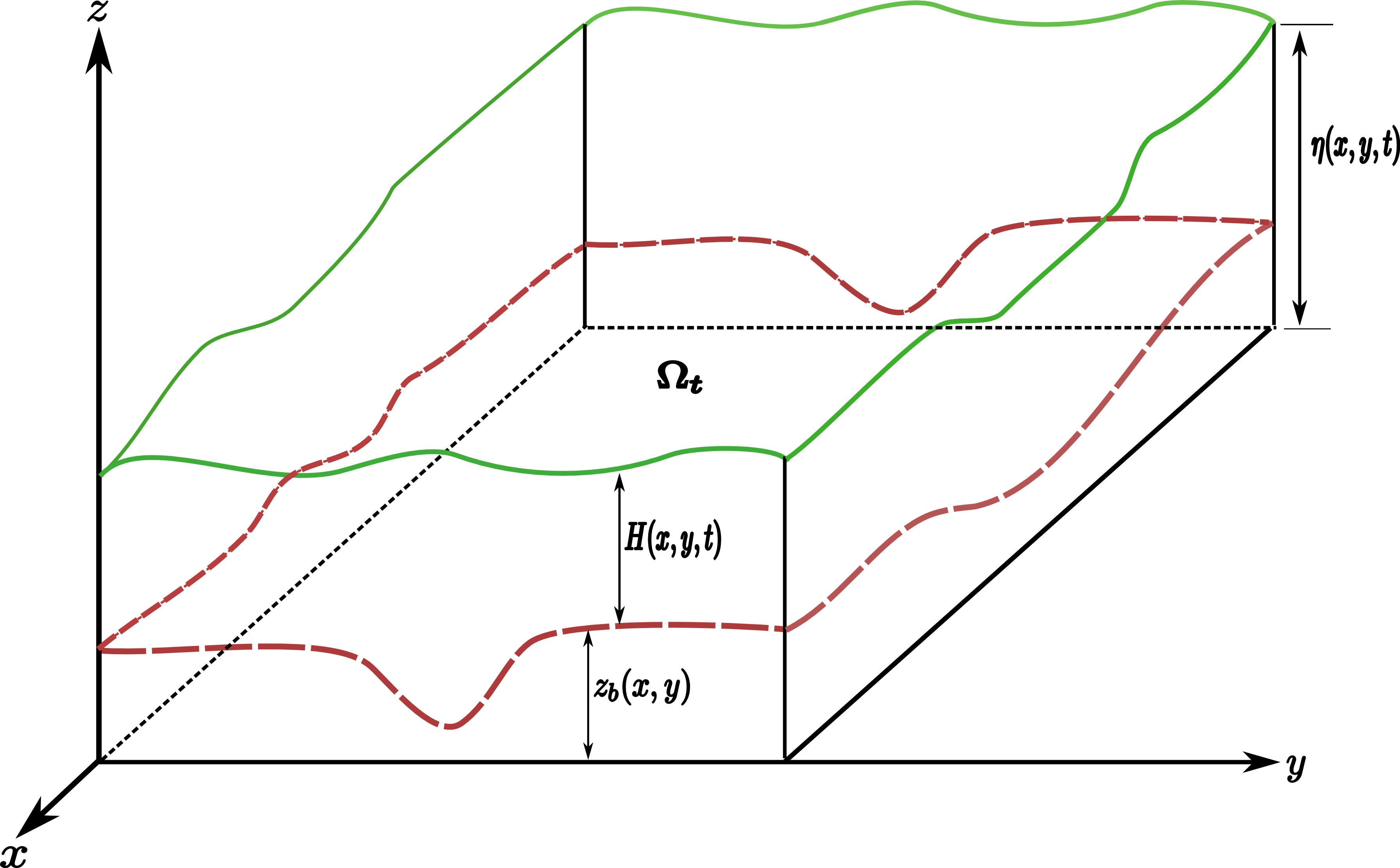
Refer to caption
Figure 1: Flow over a domain with bottom topography zb(x,y)subscript𝑧𝑏𝑥𝑦z_{b}(x,y) (dashed line) comprising of a channel and floodplain. The channel length is along the x𝑥x-axis and the width, along the y𝑦y-axis; H(x,y,t)𝐻𝑥𝑦𝑡H(x,y,t) is water depth, η(x,y,t)𝜂𝑥𝑦𝑡\eta(x,y,t), the free surface elevation, t𝑡t is time variable and (x,y,z)3(x,y,z)\in{}^{3}.
Refer to caption
(a) Flow cross section at a fixed point x𝑥x. The bottom topography comprises of the channel with bank elevations, zbl(x)subscript𝑧𝑏𝑙𝑥z_{bl}(x) and zbr(x)subscript𝑧𝑏𝑟𝑥z_{br}(x), and the floodplain which occupies the remaining regions.
Refer to caption
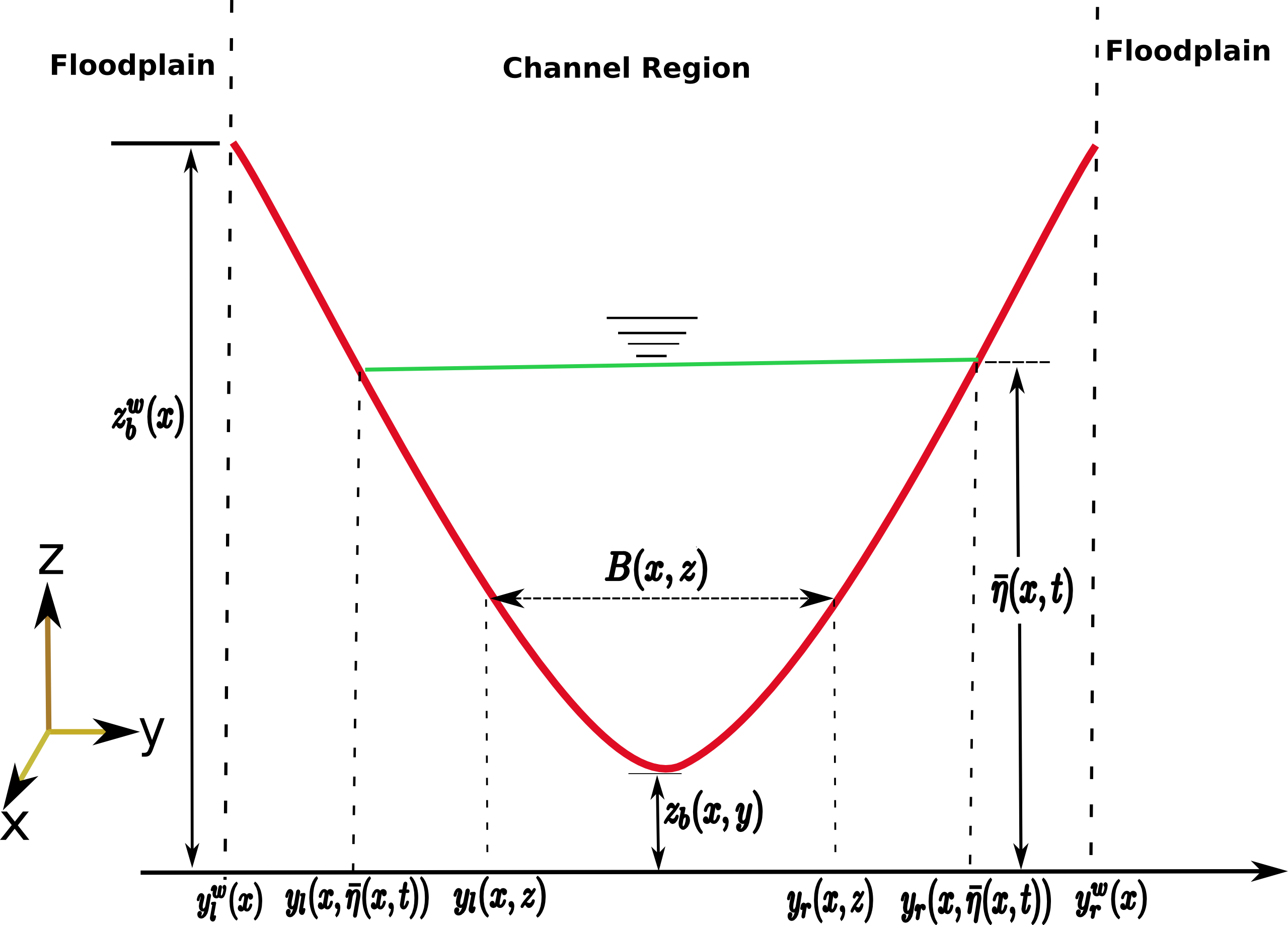
(b) Channel cross section, showing the channel wall elevation zbw(x)superscriptsubscript𝑧𝑏𝑤𝑥z_{b}^{w}(x), the top width B(x,zbw(x))𝐵𝑥superscriptsubscript𝑧𝑏𝑤𝑥B(x,z_{b}^{w}(x)), the bottom elevation in 1D sense Zb(x)subscript𝑍𝑏𝑥Z_{b}(x), laterally flat free-surface elevation η¯(x,t)¯𝜂𝑥𝑡\bar{\eta}(x,t), and the ylimit-from𝑦y-coordinates ylw(x):=yl(x,zbw(x))assignsuperscriptsubscript𝑦𝑙𝑤𝑥subscript𝑦𝑙𝑥superscriptsubscript𝑧𝑏𝑤𝑥y_{l}^{w}(x):=y_{l}(x,z_{b}^{w}(x)) and yrw(x):=yr(x,zbw(x))assignsuperscriptsubscript𝑦𝑟𝑤𝑥subscript𝑦𝑟𝑥superscriptsubscript𝑧𝑏𝑤𝑥y_{r}^{w}(x):=y_{r}(x,z_{b}^{w}(x)) respectively of the left and right lateral walls at the channel top.
Figure 2: Flow cross sections

In this section, we present the model equations for the problem under consideration. Let us begin by considering the flow of water over the fixed horizontal 2D domain, ΩH2\Omega_{H}\subset{}^{2} which consists of a channel and floodplains (see figure 1), such that the flow at time, t𝑡t occupies the 3D domain, ΩtsubscriptΩ𝑡\Omega_{t} defined by

Ωt={(𝑿,z):3𝑿=(x,y)ΩH,zb(𝑿)zη(𝑿,t)},\Omega_{t}=\{(\vec{\boldsymbol{X}},z)\in{}^{3}:\vec{\boldsymbol{X}}=(x,y)\in\Omega_{H},\,z_{b}(\vec{\boldsymbol{X}})\leq z\leq\eta(\vec{\boldsymbol{X}},t)\}, (1)

bounded below by a fixed bottom, zb(𝑿)subscript𝑧𝑏𝑿z_{b}(\vec{\boldsymbol{X}}) and above by the water free-surface elevation, η(𝑿,t)𝜂𝑿𝑡\eta(\vec{\boldsymbol{X}},t) given by

η(𝑿,t)=zb(𝑿)+H(𝑿,t)𝜂𝑿𝑡subscript𝑧𝑏𝑿𝐻𝑿𝑡\eta(\vec{\boldsymbol{X}},t)=z_{b}(\vec{\boldsymbol{X}})+H(\vec{\boldsymbol{X}},t) (2)

and H(𝑿,t)𝐻𝑿𝑡H(\vec{\boldsymbol{X}},t) is the depth of fluid at time, t𝑡t. A cross section of the flow domain is shown in figure 2(a). The length of the channel lies along the x𝑥x-axis (frontal direction) and the width, along the y𝑦y-axis (lateral direction), while zb,l(x)subscript𝑧𝑏𝑙𝑥z_{b,l}(x) and zbr(x)subscript𝑧𝑏𝑟𝑥z_{br}(x) are the left and right bank elevation of the channel, see figure 2(a). An important quantity is the maximum channel wall elevation or simply, channel wall elevation.

Definition 2.1 (Channel wall elevation, zbw(x)superscriptsubscript𝑧𝑏𝑤𝑥z_{b}^{w}(x))

The channel wall elevation at cross section x, is the minimum elevation of the channel banks above which flooding is said to have occurred. We denote it by zbw(x)superscriptsubscript𝑧𝑏𝑤𝑥z_{b}^{w}(x), that is

zbw(x)=min(zbl(x),zbr(x)),superscriptsubscript𝑧𝑏𝑤𝑥subscript𝑧𝑏𝑙𝑥subscript𝑧𝑏𝑟𝑥z_{b}^{w}(x)=\min(z_{bl}(x),z_{br}(x)), (3)

see figures 2(a) and 2(b).

That is, zbw(x)superscriptsubscript𝑧𝑏𝑤𝑥z_{b}^{w}(x) is the channel top. Figure 2(b) shows the channel cross section, depicting its geometry, including the 1D laterally constant channel bottom topography given by

Zb(x)=minyzb(x,y).subscript𝑍𝑏𝑥subscript𝑦subscript𝑧𝑏𝑥𝑦Z_{b}(x)=\min_{y}z_{b}(x,y).

It also depicts the wall elevation zbw(x)superscriptsubscript𝑧𝑏𝑤𝑥z_{b}^{w}(x), the top width B(x,zbw(x))𝐵𝑥superscriptsubscript𝑧𝑏𝑤𝑥B(x,z_{b}^{w}(x)) and the y𝑦y-coordinates, ylw(x):=yl(x,zbw(x))assignsuperscriptsubscript𝑦𝑙𝑤𝑥subscript𝑦𝑙𝑥superscriptsubscript𝑧𝑏𝑤𝑥y_{l}^{w}(x):=y_{l}(x,z_{b}^{w}(x)) and yrw(x):=yr(x,zbw(x))assignsuperscriptsubscript𝑦𝑟𝑤𝑥subscript𝑦𝑟𝑥superscriptsubscript𝑧𝑏𝑤𝑥y_{r}^{w}(x):=y_{r}(x,z_{b}^{w}(x)) of the left and right boundaries at the top, where B(x,z)𝐵𝑥𝑧B(x,z) gives the channel width at an elevation z𝑧z above a reference elevation z𝑧z, and yl(x,z)subscript𝑦𝑙𝑥𝑧y_{l}(x,z) and yr(x,z)subscript𝑦𝑟𝑥𝑧y_{r}(x,z) are the ylimit-from𝑦y-coordinates of the left and right lateral boundaries, respectively, at elevation z𝑧z. So that

B(x,z)=yr(x,z)yl(x,z)z,𝐵𝑥𝑧subscript𝑦𝑟𝑥𝑧subscript𝑦𝑙𝑥𝑧for-all𝑧B(x,z)=y_{r}(x,z)-y_{l}(x,z)\quad\forall z, (4)

such that

yr(x,z)=yl(x,z),B(x,z)=0 for all z<Zb(x);formulae-sequencesubscript𝑦𝑟𝑥𝑧subscript𝑦𝑙𝑥𝑧formulae-sequence𝐵𝑥𝑧0 for all 𝑧subscript𝑍𝑏𝑥y_{r}(x,z)=y_{l}(x,z),\quad B(x,z)=0\quad\mbox{ for all }z<Z_{b}(x); (5)

and the bottom elevation satisfies

zb(𝑿)|y=yl(x,z),yr(x,z)=zz[Zb(x),zbw(x)],formulae-sequenceevaluated-atsubscript𝑧𝑏𝑿𝑦subscript𝑦𝑙𝑥𝑧subscript𝑦𝑟𝑥𝑧𝑧for-all𝑧subscript𝑍𝑏𝑥superscriptsubscript𝑧𝑏𝑤𝑥\displaystyle z_{b}(\vec{\boldsymbol{X}})|_{y=y_{l}(x,z),y_{r}(x,z)}=z\quad\forall z\in[Z_{b}(x),z_{b}^{w}(x)], (6)

see figure 2(b). Furthermore, we extend the definition of the width functions above the channel top (z>zbw(x)𝑧superscriptsubscript𝑧𝑏𝑤𝑥z>z_{b}^{w}(x)) in the following:

yl,r(x,z)=yl,rw(x),B(x,z)=B(x,zbw(x))zzbw(x),formulae-sequencesubscript𝑦𝑙𝑟𝑥𝑧superscriptsubscript𝑦𝑙𝑟𝑤𝑥formulae-sequence𝐵𝑥𝑧𝐵𝑥superscriptsubscript𝑧𝑏𝑤𝑥for-all𝑧superscriptsubscript𝑧𝑏𝑤𝑥\displaystyle y_{l,r}(x,z)=y_{l,r}^{w}(x),\quad B(x,z)=B(x,z_{b}^{w}(x))\quad\forall z\geq z_{b}^{w}(x), (7)

see figure 2(b).

The flow cross section, <y<𝑦-\infty<y<\infty in 2(a) has been partitioned into (i) the channel cross section, ylw(x)yyrw(x)superscriptsubscript𝑦𝑙𝑤𝑥𝑦superscriptsubscript𝑦𝑟𝑤𝑥y_{l}^{w}(x)\leq y\leq y_{r}^{w}(x) and (ii) the floodplains, <yylw(x)𝑦superscriptsubscript𝑦𝑙𝑤𝑥-\infty<y\leq y_{l}^{w}(x) and yrw(x)y<superscriptsubscript𝑦𝑟𝑤𝑥𝑦y_{r}^{w}(x)\leq y<-\infty, see figure 2(b). The flow in the floodplains is simulated with the standard 2D shallow water models (see section 2.3), therefore we focus on deriving the model equations for the flow in the channel.

With the channel geometry completely defined, we now consider the initial flow condition. In general, the free surface elevation η(𝑿,t)𝜂𝑿𝑡\eta(\vec{\boldsymbol{X}},t) is 2D, see figures 1 and 2(a). However, we assume that it is always 1D (laterally constant and given by η¯(x,t)¯𝜂𝑥𝑡\bar{\eta}(x,t)) within the channel, see figure 2(b)). Hence, we say the channel is full whenever

η¯(x,t)>zbw(x).¯𝜂𝑥𝑡superscriptsubscript𝑧𝑏𝑤𝑥\bar{\eta}(x,t)>z_{b}^{w}(x). (8)

Note that in general, the channel flow lateral boundaries are at the coordinates, yl,r(x,η¯(x,t))subscript𝑦𝑙𝑟𝑥¯𝜂𝑥𝑡y_{l,r}(x,\bar{\eta}(x,t)), not yl,rw(x)superscriptsubscript𝑦𝑙𝑟𝑤𝑥y_{l,r}^{w}(x), see figures 2(b) and 3(a). These two sets of coordinates are only equal if the channel is full, see (7) and also figure 2(b). They are not equal if the channel is not full, see figure 3(a). If the channel is not full (η¯(x,t)zbw(x)¯𝜂𝑥𝑡superscriptsubscript𝑧𝑏𝑤𝑥\bar{\eta}(x,t)\leq z_{b}^{w}(x)), then the water height and velocities are zero at the top lateral boundaries, that is

(u(𝑿,z,t),v(𝑿,z,t),w(𝑿,z,t),H(𝑿,t))|y=yl,rw(x)=0 whenever η¯(x,t)zbw(x),formulae-sequenceevaluated-at𝑢𝑿𝑧𝑡𝑣𝑿𝑧𝑡𝑤𝑿𝑧𝑡𝐻𝑿𝑡𝑦superscriptsubscript𝑦𝑙𝑟𝑤𝑥0 whenever ¯𝜂𝑥𝑡superscriptsubscript𝑧𝑏𝑤𝑥\displaystyle\bigg{(}u(\vec{\boldsymbol{X}},z,t),v(\vec{\boldsymbol{X}},z,t),w(\vec{\boldsymbol{X}},z,t),H(\vec{\boldsymbol{X}},t)\bigg{)}\bigg{|}_{y=y_{l,r}^{w}(x)}=0\quad\mbox{ whenever }\bar{\eta}(x,t)\leq z_{b}^{w}(x), (9)

(see figure 3(a)) where u,v,w𝑢𝑣𝑤u,v,w are velocity components along the x,y,z𝑥𝑦𝑧x,y,z directions respectively.

2.2 Derivation of the channel flow model with coupling term

Under the assumption of compressible and inviscid fluid, the flow of water in the channel is governed by the following 3D Free-Surface Euler Equations [10]:

xu(𝑿,z,t)+yv(𝑿,z,t)+zw(𝑿,z,t)=0.subscript𝑥𝑢𝑿𝑧𝑡subscript𝑦𝑣𝑿𝑧𝑡subscript𝑧𝑤𝑿𝑧𝑡0\displaystyle\begin{split}\partial_{x}u(\vec{\boldsymbol{X}},z,t)+\partial_{y}v(\vec{\boldsymbol{X}},z,t)+\partial_{z}w(\vec{\boldsymbol{X}},z,t)=0.\end{split} (10)
tu(𝑿,z,t)+u(𝑿,z,t)xu(𝑿,z,t)+v(𝑿,z,t)yu(𝑿,z,t)+w(𝑿,z,t)zu(𝑿,z,t)=1ρxP(𝑿,z,t).subscript𝑡𝑢𝑿𝑧𝑡𝑢𝑿𝑧𝑡subscript𝑥𝑢𝑿𝑧𝑡𝑣𝑿𝑧𝑡subscript𝑦𝑢𝑿𝑧𝑡𝑤𝑿𝑧𝑡subscript𝑧𝑢𝑿𝑧𝑡1𝜌subscript𝑥𝑃𝑿𝑧𝑡\displaystyle\begin{split}\partial_{t}u(\vec{\boldsymbol{X}},z,t)+u(\vec{\boldsymbol{X}},z,t)\partial_{x}u(\vec{\boldsymbol{X}},z,t)+v(\vec{\boldsymbol{X}},z,t)\partial_{y}u(\vec{\boldsymbol{X}},z,t)+w(\vec{\boldsymbol{X}},z,t)\partial_{z}u(\vec{\boldsymbol{X}},z,t)=-\frac{1}{\rho}\partial_{x}P(\vec{\boldsymbol{X}},z,t).\end{split} (11)
tv(𝑿,z,t)+u(𝑿,z,t)xv(𝑿,z,t)+v(𝑿,z,t)yv(𝑿,z,t)+w(𝑿,z,t)zv(𝑿,z,t)=1ρyP(𝑿,z,t).subscript𝑡𝑣𝑿𝑧𝑡𝑢𝑿𝑧𝑡subscript𝑥𝑣𝑿𝑧𝑡𝑣𝑿𝑧𝑡subscript𝑦𝑣𝑿𝑧𝑡𝑤𝑿𝑧𝑡subscript𝑧𝑣𝑿𝑧𝑡1𝜌subscript𝑦𝑃𝑿𝑧𝑡\displaystyle\begin{split}\partial_{t}v(\vec{\boldsymbol{X}},z,t)+u(\vec{\boldsymbol{X}},z,t)\partial_{x}v(\vec{\boldsymbol{X}},z,t)+v(\vec{\boldsymbol{X}},z,t)\partial_{y}v(\vec{\boldsymbol{X}},z,t)+w(\vec{\boldsymbol{X}},z,t)\partial_{z}v(\vec{\boldsymbol{X}},z,t)=-\frac{1}{\rho}\partial_{y}P(\vec{\boldsymbol{X}},z,t).\end{split} (12)
tw(𝑿,z,t)+u(𝑿,z,t)xw(𝑿,z,t)+v(𝑿,z,t)yw(𝑿,z,t)+w(𝑿,z,t)zw(𝑿,z,t)=1ρxP(𝑿,z,t)g.subscript𝑡𝑤𝑿𝑧𝑡𝑢𝑿𝑧𝑡subscript𝑥𝑤𝑿𝑧𝑡𝑣𝑿𝑧𝑡subscript𝑦𝑤𝑿𝑧𝑡𝑤𝑿𝑧𝑡subscript𝑧𝑤𝑿𝑧𝑡1𝜌subscript𝑥𝑃𝑿𝑧𝑡𝑔\displaystyle\begin{split}\partial_{t}w(\vec{\boldsymbol{X}},z,t)+u(\vec{\boldsymbol{X}},z,t)\partial_{x}w(\vec{\boldsymbol{X}},z,t)+v(\vec{\boldsymbol{X}},z,t)\partial_{y}w(\vec{\boldsymbol{X}},z,t)+w(\vec{\boldsymbol{X}},z,t)\partial_{z}w(\vec{\boldsymbol{X}},z,t)\\ =-\frac{1}{\rho}\partial_{x}P(\vec{\boldsymbol{X}},z,t)-g.\end{split} (13)
(u(𝑿,z,t)xzb(𝑿)+v(𝑿,z,t)yzb(𝑿)w(𝑿,z,t))|z=zb(𝑿)=0.evaluated-at𝑢𝑿𝑧𝑡subscript𝑥subscript𝑧𝑏𝑿𝑣𝑿𝑧𝑡subscript𝑦subscript𝑧𝑏𝑿𝑤𝑿𝑧𝑡𝑧subscript𝑧𝑏𝑿0\displaystyle\begin{split}\left(u(\vec{\boldsymbol{X}},z,t)\partial_{x}z_{b}(\vec{\boldsymbol{X}})+v(\vec{\boldsymbol{X}},z,t)\partial_{y}z_{b}(\vec{\boldsymbol{X}})-w(\vec{\boldsymbol{X}},z,t)\right)\bigg{|}_{z=z_{b}(\vec{\boldsymbol{X}})}=0.\end{split} (14)
(tη(𝑿,t)+u(𝑿,z,t)xη(𝑿,t)+v(𝑿,z,t)yη(𝑿,t)w(𝑿,z,t))|z=η(𝑿,t)=0.evaluated-atsubscript𝑡𝜂𝑿𝑡𝑢𝑿𝑧𝑡subscript𝑥𝜂𝑿𝑡𝑣𝑿𝑧𝑡subscript𝑦𝜂𝑿𝑡𝑤𝑿𝑧𝑡𝑧𝜂𝑿𝑡0\displaystyle\begin{split}\left(\partial_{t}\eta(\vec{\boldsymbol{X}},t)+u(\vec{\boldsymbol{X}},z,t)\partial_{x}\eta(\vec{\boldsymbol{X}},t)+v(\vec{\boldsymbol{X}},z,t)\partial_{y}\eta(\vec{\boldsymbol{X}},t)-w(\vec{\boldsymbol{X}},z,t)\right)\bigg{|}_{z=\eta(\vec{\boldsymbol{X}},t)}=0.\end{split} (15)
P(𝑿,z,t)=Patm on z=η(𝑿,t),formulae-sequence𝑃𝑿𝑧𝑡subscript𝑃𝑎𝑡𝑚 on 𝑧𝜂𝑿𝑡P(\vec{\boldsymbol{X}},z,t)=P_{atm}\quad\mbox{ on }z=\eta(\vec{\boldsymbol{X}},t), (16)

where ρ,(u,v,w)T𝜌superscript𝑢𝑣𝑤𝑇\rho,(u,v,w)^{T} and P𝑃P are the fluid density, velocity vector and pressure at point (𝑿,z)𝑿𝑧(\vec{\boldsymbol{X}},z) at time, t𝑡t and Patmsubscript𝑃𝑎𝑡𝑚P_{atm} is the atmospheric pressure, which is usually conveniently taken to be zero.

The flow quantities of interest in the 1D channel model are the wetted cross sectional area, A(x,t)𝐴𝑥𝑡A(x,t) and the section averaged discharge, Q(x,t)𝑄𝑥𝑡Q(x,t) given by the following averages:

Q(x,t)𝑄𝑥𝑡\displaystyle Q(x,t) =yl(x,η¯(x,t))yr(x,η¯(x,t))zb(𝑿)η¯(x,t)u(𝑿,z,t)𝑑z𝑑y,absentsuperscriptsubscriptsubscript𝑦𝑙𝑥¯𝜂𝑥𝑡subscript𝑦𝑟𝑥¯𝜂𝑥𝑡superscriptsubscriptsubscript𝑧𝑏𝑿¯𝜂𝑥𝑡𝑢𝑿𝑧𝑡differential-d𝑧differential-d𝑦\displaystyle=\int_{y_{l}(x,\bar{\eta}(x,t))}^{y_{r}(x,\bar{\eta}(x,t))}\int_{z_{b}(\vec{\boldsymbol{X}})}^{\bar{\eta}(x,t)}u(\vec{\boldsymbol{X}},z,t)dzdy, (17)
A(x,t)𝐴𝑥𝑡\displaystyle A(x,t) =yl(x,η¯(x,t))yr(x,η¯(x,t))zb(𝑿)η¯(x,t)𝑑z𝑑y=yl(x,η¯(x,t))yr(x,η¯(x,t))H(𝑿,t)𝑑y.absentsuperscriptsubscriptsubscript𝑦𝑙𝑥¯𝜂𝑥𝑡subscript𝑦𝑟𝑥¯𝜂𝑥𝑡superscriptsubscriptsubscript𝑧𝑏𝑿¯𝜂𝑥𝑡differential-d𝑧differential-d𝑦superscriptsubscriptsubscript𝑦𝑙𝑥¯𝜂𝑥𝑡subscript𝑦𝑟𝑥¯𝜂𝑥𝑡𝐻𝑿𝑡differential-d𝑦\displaystyle=\int_{y_{l}(x,\bar{\eta}(x,t))}^{y_{r}(x,\bar{\eta}(x,t))}\int_{z_{b}(\vec{\boldsymbol{X}})}^{\bar{\eta}(x,t)}dzdy=\int_{y_{l}(x,\bar{\eta}(x,t))}^{y_{r}(x,\bar{\eta}(x,t))}H(\vec{\boldsymbol{X}},t)dy. (18)

So that the section-averaged velocity, u¯¯𝑢\underline{u} is given as

u¯(x,t)=Q(x,t)A(x,t)=1A(x,t)yl(x,η¯(x,t))yr(x,η¯(x,t))zb(𝑿)η¯(x,t)u(𝑿,z,t)𝑑z𝑑y.¯𝑢𝑥𝑡𝑄𝑥𝑡𝐴𝑥𝑡1𝐴𝑥𝑡superscriptsubscriptsubscript𝑦𝑙𝑥¯𝜂𝑥𝑡subscript𝑦𝑟𝑥¯𝜂𝑥𝑡superscriptsubscriptsubscript𝑧𝑏𝑿¯𝜂𝑥𝑡𝑢𝑿𝑧𝑡differential-d𝑧differential-d𝑦\underline{u}(x,t)=\frac{Q(x,t)}{A(x,t)}=\frac{1}{A(x,t)}\int_{y_{l}(x,\bar{\eta}(x,t))}^{y_{r}(x,\bar{\eta}(x,t))}\int_{z_{b}(\vec{\boldsymbol{X}})}^{\bar{\eta}(x,t)}u(\vec{\boldsymbol{X}},z,t)dzdy. (19)

First, we note that y𝑦y-independence of the free-surface, η¯(x,t)¯𝜂𝑥𝑡\bar{\eta}(x,t) means that the sum,

H(𝑿,t)+zb(𝑿)=η¯(x,t),yl(x,η¯(x,t))yyr(x,η¯(x,t)),formulae-sequence𝐻𝑿𝑡subscript𝑧𝑏𝑿¯𝜂𝑥𝑡for-allsubscript𝑦𝑙𝑥¯𝜂𝑥𝑡𝑦subscript𝑦𝑟𝑥¯𝜂𝑥𝑡H(\vec{\boldsymbol{X}},t)+z_{b}(\vec{\boldsymbol{X}})=\bar{\eta}(x,t),\quad\forall y_{l}(x,\bar{\eta}(x,t))\leq y\leq y_{r}(x,\bar{\eta}(x,t)), (20)

is constant in y𝑦y, even though each of H(𝑿,t)𝐻𝑿𝑡H(\vec{\boldsymbol{X}},t) and zb(𝑿)subscript𝑧𝑏𝑿z_{b}(\vec{\boldsymbol{X}}) depends on y𝑦y, see figures 2(b) and 3(a).

The shallow water assumption that water depth is small compared to horizontal length leads to neglect vertical acceleration, hence the z-momentum equation, (13) and the dynamic boundary condition, (16), lead to the following hydrostatic pressure:

P(𝑿,z,t)=ρg(η¯(x,t)z)xP(𝑿,z,t)=ρgxη¯(x,t).\displaystyle P(\vec{\boldsymbol{X}},z,t)=\rho g(\bar{\eta}(x,t)-z)\quad\Longrightarrow\partial_{x}P(\vec{\boldsymbol{X}},z,t)=\rho g\partial_{x}\bar{\eta}(x,t).

Therefore, the FSEE (10) -(16), reduce to the following system:

xu(𝑿,z,t)+yv(𝑿,z,t)+zw(𝑿,z,t)=0.subscript𝑥𝑢𝑿𝑧𝑡subscript𝑦𝑣𝑿𝑧𝑡subscript𝑧𝑤𝑿𝑧𝑡0\displaystyle\partial_{x}u(\vec{\boldsymbol{X}},z,t)+\partial_{y}v(\vec{\boldsymbol{X}},z,t)+\partial_{z}w(\vec{\boldsymbol{X}},z,t)=0. (21)
tu(𝑿,z,t)+x(u2(𝑿,z,t))+y(u(𝑿,z,t)v(𝑿,z,t))+z(u(𝑿,z,t)w(𝑿,z,t))=gxη¯(x,t).subscript𝑡𝑢𝑿𝑧𝑡subscript𝑥superscript𝑢2𝑿𝑧𝑡subscript𝑦𝑢𝑿𝑧𝑡𝑣𝑿𝑧𝑡subscript𝑧𝑢𝑿𝑧𝑡𝑤𝑿𝑧𝑡𝑔subscript𝑥¯𝜂𝑥𝑡\displaystyle\partial_{t}u(\vec{\boldsymbol{X}},z,t)+\partial_{x}\left(u^{2}(\vec{\boldsymbol{X}},z,t)\right)+\partial_{y}\left(u(\vec{\boldsymbol{X}},z,t)v(\vec{\boldsymbol{X}},z,t)\right)+\partial_{z}\left(u(\vec{\boldsymbol{X}},z,t)w(\vec{\boldsymbol{X}},z,t)\right)=-g\partial_{x}\bar{\eta}(x,t). (22)
(u(𝑿,z,t)xzb(𝑿)+v(𝑿,z,t)yzb(𝑿)w(𝑿,z,t))|z=zb(𝑿)=0.evaluated-at𝑢𝑿𝑧𝑡subscript𝑥subscript𝑧𝑏𝑿𝑣𝑿𝑧𝑡subscript𝑦subscript𝑧𝑏𝑿𝑤𝑿𝑧𝑡𝑧subscript𝑧𝑏𝑿0\displaystyle\left(u(\vec{\boldsymbol{X}},z,t)\partial_{x}z_{b}(\vec{\boldsymbol{X}})+v(\vec{\boldsymbol{X}},z,t)\partial_{y}z_{b}(\vec{\boldsymbol{X}})-w(\vec{\boldsymbol{X}},z,t)\right)\bigg{|}_{z=z_{b}(\vec{\boldsymbol{X}})}=0. (23)
(tη¯(x,t)+u(𝑿,z,t)xη¯(x,t)w(𝑿,z,t))|z=η¯(x,t)=0.evaluated-atsubscript𝑡¯𝜂𝑥𝑡𝑢𝑿𝑧𝑡subscript𝑥¯𝜂𝑥𝑡𝑤𝑿𝑧𝑡𝑧¯𝜂𝑥𝑡0\displaystyle\left(\partial_{t}\bar{\eta}(x,t)+u(\vec{\boldsymbol{X}},z,t)\partial_{x}\bar{\eta}(x,t)-w(\vec{\boldsymbol{X}},z,t)\right)\bigg{|}_{z=\bar{\eta}(x,t)}=0. (24)

Integrating (21) vertically (over zb(𝑿)zη¯subscript𝑧𝑏𝑿𝑧¯𝜂z_{b}(\vec{\boldsymbol{X}})\leq z\leq\bar{\eta}), and laterally (over yl(x,η¯(x,t))yyr(x,η¯(x,t))subscript𝑦𝑙𝑥¯𝜂𝑥𝑡𝑦subscript𝑦𝑟𝑥¯𝜂𝑥𝑡y_{l}(x,\bar{\eta}(x,t))\leq y\leq y_{r}(x,\bar{\eta}(x,t))), applying the Leibnitz rule and using the kinematic boundary conditions, (23), (24), we have the following mass equation (25) below see [12]. Repeating the same process for (22), gives the discharge equation (26) below:

tA(x,t)+xQ(x,t)subscript𝑡𝐴𝑥𝑡subscript𝑥𝑄𝑥𝑡\displaystyle\partial_{t}A(x,t)+\partial_{x}Q(x,t) =ΦA(x,t),absentsuperscriptΦ𝐴𝑥𝑡\displaystyle=\Phi^{A}(x,t), (25)
tQ(x,t)+x(Q2(x,t)A(x,t))subscript𝑡𝑄𝑥𝑡subscript𝑥superscript𝑄2𝑥𝑡𝐴𝑥𝑡\displaystyle\partial_{t}Q(x,t)+\partial_{x}\left(\frac{Q^{2}(x,t)}{A(x,t)}\right) =gA(x,t)xη¯(x,t)+ΦQ(x,t),absent𝑔𝐴𝑥𝑡subscript𝑥¯𝜂𝑥𝑡superscriptΦ𝑄𝑥𝑡\displaystyle=-gA(x,t)\partial_{x}\bar{\eta}(x,t)+\Phi^{Q}(x,t), (26)

see [17, 12] for details; ΦA(x,t)superscriptΦ𝐴𝑥𝑡\Phi^{A}(x,t) and ΦQ(x,t)superscriptΦ𝑄𝑥𝑡\Phi^{Q}(x,t) are the coupling terms defined as

ΦA(x,t)=xyr(x,η¯(x,t))[zb(𝑿)η¯(x,t)u(𝑿,z,t)𝑑z]y=yr(x,η¯(x,t))[zb(𝑿)η¯(x,t)v(𝑿,z,t)𝑑z]y=yr(x,η¯(x,t))xyl(x,η¯(x,t))[zb(𝑿)η¯(x,t)u(𝑿,z,t)𝑑z]y=yl(x,η¯(x,t))+[zb(𝑿)η¯(x,t)v(𝑿,z,t)𝑑z]y=yl(x,η¯(x,t)).superscriptΦ𝐴𝑥𝑡subscript𝑥subscript𝑦𝑟𝑥¯𝜂𝑥𝑡subscriptdelimited-[]superscriptsubscriptsubscript𝑧𝑏𝑿¯𝜂𝑥𝑡𝑢𝑿𝑧𝑡differential-d𝑧𝑦subscript𝑦𝑟𝑥¯𝜂𝑥𝑡subscriptdelimited-[]superscriptsubscriptsubscript𝑧𝑏𝑿¯𝜂𝑥𝑡𝑣𝑿𝑧𝑡differential-d𝑧𝑦subscript𝑦𝑟𝑥¯𝜂𝑥𝑡subscript𝑥subscript𝑦𝑙𝑥¯𝜂𝑥𝑡subscriptdelimited-[]superscriptsubscriptsubscript𝑧𝑏𝑿¯𝜂𝑥𝑡𝑢𝑿𝑧𝑡differential-d𝑧𝑦subscript𝑦𝑙𝑥¯𝜂𝑥𝑡subscriptdelimited-[]superscriptsubscriptsubscript𝑧𝑏𝑿¯𝜂𝑥𝑡𝑣𝑿𝑧𝑡differential-d𝑧𝑦subscript𝑦𝑙𝑥¯𝜂𝑥𝑡\displaystyle\begin{split}\Phi^{A}(x,t)&=\partial_{x}y_{r}(x,\bar{\eta}(x,t))\left[\int_{z_{b}(\vec{\boldsymbol{X}})}^{\bar{\eta}(x,t)}u(\vec{\boldsymbol{X}},z,t)dz\right]_{y=y_{r}(x,\bar{\eta}(x,t))}-\left[\int_{z_{b}(\vec{\boldsymbol{X}})}^{\bar{\eta}(x,t)}v(\vec{\boldsymbol{X}},z,t)dz\right]_{y=y_{r}(x,\bar{\eta}(x,t))}\\ &-\partial_{x}y_{l}(x,\bar{\eta}(x,t))\left[\int_{z_{b}(\vec{\boldsymbol{X}})}^{\bar{\eta}(x,t)}u(\vec{\boldsymbol{X}},z,t)dz\right]_{y=y_{l}(x,\bar{\eta}(x,t))}+\left[\int_{z_{b}(\vec{\boldsymbol{X}})}^{\bar{\eta}(x,t)}v(\vec{\boldsymbol{X}},z,t)dz\right]_{y=y_{l}(x,\bar{\eta}(x,t))}.\end{split} (27)
ΦQ(x,t)=xyr(x,η¯(x,t))[zb(𝑿)η¯(x,t)u2(𝑿,z,t)𝑑z]y=yr(x,η¯(x,t))[zb(𝑿)η¯(x,t)u(𝑿,z,t)v(𝑿,z,t)𝑑z]y=yr(x,η¯(x,t))xyl(x,η¯(x,t))[zb(𝑿)η¯(x,t)u2(𝑿,z,t)𝑑z]y=yl(x,η¯(x,t))+[zb(𝑿)η¯(x,t)u(𝑿,z,t)v(𝑿,z,t)𝑑z]y=yl(x,η¯(x,t)).superscriptΦ𝑄𝑥𝑡subscript𝑥subscript𝑦𝑟𝑥¯𝜂𝑥𝑡subscriptdelimited-[]superscriptsubscriptsubscript𝑧𝑏𝑿¯𝜂𝑥𝑡superscript𝑢2𝑿𝑧𝑡differential-d𝑧𝑦subscript𝑦𝑟𝑥¯𝜂𝑥𝑡subscriptdelimited-[]superscriptsubscriptsubscript𝑧𝑏𝑿¯𝜂𝑥𝑡𝑢𝑿𝑧𝑡𝑣𝑿𝑧𝑡differential-d𝑧𝑦subscript𝑦𝑟𝑥¯𝜂𝑥𝑡subscript𝑥subscript𝑦𝑙𝑥¯𝜂𝑥𝑡subscriptdelimited-[]superscriptsubscriptsubscript𝑧𝑏𝑿¯𝜂𝑥𝑡superscript𝑢2𝑿𝑧𝑡differential-d𝑧𝑦subscript𝑦𝑙𝑥¯𝜂𝑥𝑡subscriptdelimited-[]superscriptsubscriptsubscript𝑧𝑏𝑿¯𝜂𝑥𝑡𝑢𝑿𝑧𝑡𝑣𝑿𝑧𝑡differential-d𝑧𝑦subscript𝑦𝑙𝑥¯𝜂𝑥𝑡\displaystyle\begin{split}\Phi^{Q}(x,t)&=\partial_{x}y_{r}(x,\bar{\eta}(x,t))\left[\int_{z_{b}(\vec{\boldsymbol{X}})}^{\bar{\eta}(x,t)}u^{2}(\vec{\boldsymbol{X}},z,t)dz\right]_{y=y_{r}(x,\bar{\eta}(x,t))}-\left[\int_{z_{b}(\vec{\boldsymbol{X}})}^{\bar{\eta}(x,t)}u(\vec{\boldsymbol{X}},z,t)v(\vec{\boldsymbol{X}},z,t)dz\right]_{y=y_{r}(x,\bar{\eta}(x,t))}\\ &-\partial_{x}y_{l}(x,\bar{\eta}(x,t))\left[\int_{z_{b}(\vec{\boldsymbol{X}})}^{\bar{\eta}(x,t)}u^{2}(\vec{\boldsymbol{X}},z,t)dz\right]_{y=y_{l}(x,\bar{\eta}(x,t))}+\left[\int_{z_{b}(\vec{\boldsymbol{X}})}^{\bar{\eta}(x,t)}u(\vec{\boldsymbol{X}},z,t)v(\vec{\boldsymbol{X}},z,t)dz\right]_{y=y_{l}(x,\bar{\eta}(x,t))}.\end{split} (28)

Note that if the channel is not full, then we have ΦA(x,t)=0superscriptΦ𝐴𝑥𝑡0\Phi^{A}(x,t)=0 and ΦQ(x,t)=0superscriptΦ𝑄𝑥𝑡0\Phi^{Q}(x,t)=0 because non-full channel means η¯(x,t)zbw(x)zb(x,yl,r(x,η¯(x,t)))=η¯(x,t)¯𝜂𝑥𝑡superscriptsubscript𝑧𝑏𝑤𝑥subscript𝑧𝑏𝑥subscript𝑦𝑙𝑟𝑥¯𝜂𝑥𝑡¯𝜂𝑥𝑡\bar{\eta}(x,t)\leq z_{b}^{w}(x)\Longrightarrow z_{b}(x,y_{l,r}(x,\bar{\eta}(x,t)))=\bar{\eta}(x,t) by (6). Hence, both limits in all the integrals in (27)-(28), so the coupling terms vanish. In this case, the model, (25)-(26) reduces to the standard 1D Saint-Venant Models.

It is straight forward to show that

xyl,r(x,η¯(x,t))[zb(𝑿)η¯(x,t)θ(𝑿,z,t)𝑑z]y=yl,r(x,η¯(x,t))=xyl,rw(x)[zb(𝑿)η¯(x,t)θ(𝑿,z,t)𝑑z]y=yl,rw(x)subscript𝑥subscript𝑦𝑙𝑟𝑥¯𝜂𝑥𝑡subscriptdelimited-[]superscriptsubscriptsubscript𝑧𝑏𝑿¯𝜂𝑥𝑡𝜃𝑿𝑧𝑡differential-d𝑧𝑦subscript𝑦𝑙𝑟𝑥¯𝜂𝑥𝑡subscript𝑥superscriptsubscript𝑦𝑙𝑟𝑤𝑥subscriptdelimited-[]superscriptsubscriptsubscript𝑧𝑏𝑿¯𝜂𝑥𝑡𝜃𝑿𝑧𝑡differential-d𝑧𝑦superscriptsubscript𝑦𝑙𝑟𝑤𝑥\partial_{x}y_{l,r}(x,\bar{\eta}(x,t))\bigg{[}\int_{z_{b}(\vec{\boldsymbol{X}})}^{\bar{\eta}(x,t)}\theta(\vec{\boldsymbol{X}},z,t)dz\bigg{]}_{y=y_{l,r}(x,\bar{\eta}(x,t))}=\partial_{x}y_{l,r}^{w}(x)\bigg{[}\int_{z_{b}(\vec{\boldsymbol{X}})}^{\bar{\eta}(x,t)}\theta(\vec{\boldsymbol{X}},z,t)dz\bigg{]}_{y=y_{l,r}^{w}(x)}

where θ𝜃\theta is any of the integrands appearing in (27)-(28). Therefore, we can conveniently write the coupling terms as follows:

ΦA(x,t)=xyrw(x)[zb(𝑿)η¯(x,t)u(𝑿,z,t)𝑑z]y=yrw(x)[zb(𝑿)η¯(x,t)v(𝑿,z,t)𝑑z]y=yrw(x)xylw(x)[zb(𝑿)η¯(x,t)u(𝑿,z,t)𝑑z]y=ylw(x)+[zb(𝑿)η¯(x,t)v(𝑿,z,t)𝑑z]y=ylw(x).superscriptΦ𝐴𝑥𝑡subscript𝑥superscriptsubscript𝑦𝑟𝑤𝑥subscriptdelimited-[]superscriptsubscriptsubscript𝑧𝑏𝑿¯𝜂𝑥𝑡𝑢𝑿𝑧𝑡differential-d𝑧𝑦superscriptsubscript𝑦𝑟𝑤𝑥subscriptdelimited-[]superscriptsubscriptsubscript𝑧𝑏𝑿¯𝜂𝑥𝑡𝑣𝑿𝑧𝑡differential-d𝑧𝑦superscriptsubscript𝑦𝑟𝑤𝑥subscript𝑥superscriptsubscript𝑦𝑙𝑤𝑥subscriptdelimited-[]superscriptsubscriptsubscript𝑧𝑏𝑿¯𝜂𝑥𝑡𝑢𝑿𝑧𝑡differential-d𝑧𝑦superscriptsubscript𝑦𝑙𝑤𝑥subscriptdelimited-[]superscriptsubscriptsubscript𝑧𝑏𝑿¯𝜂𝑥𝑡𝑣𝑿𝑧𝑡differential-d𝑧𝑦superscriptsubscript𝑦𝑙𝑤𝑥\displaystyle\begin{split}\Phi^{A}(x,t)&=\partial_{x}y_{r}^{w}(x)\left[\int_{z_{b}(\vec{\boldsymbol{X}})}^{\bar{\eta}(x,t)}u(\vec{\boldsymbol{X}},z,t)dz\right]_{y=y_{r}^{w}(x)}-\left[\int_{z_{b}(\vec{\boldsymbol{X}})}^{\bar{\eta}(x,t)}v(\vec{\boldsymbol{X}},z,t)dz\right]_{y=y_{r}^{w}(x)}\\ &-\partial_{x}y_{l}^{w}(x)\left[\int_{z_{b}(\vec{\boldsymbol{X}})}^{\bar{\eta}(x,t)}u(\vec{\boldsymbol{X}},z,t)dz\right]_{y=y_{l}^{w}(x)}+\left[\int_{z_{b}(\vec{\boldsymbol{X}})}^{\bar{\eta}(x,t)}v(\vec{\boldsymbol{X}},z,t)dz\right]_{y=y_{l}^{w}(x)}.\end{split} (29)
ΦQ(x,t)=xyrw(x)[zb(𝑿)η¯(x,t)u2(𝑿,z,t)𝑑z]y=yrw(x)[zb(𝑿)η¯(x,t)u(𝑿,z,t)v(𝑿,z,t)𝑑z]y=yrw(x)xylw(x)[zb(𝑿)η¯(x,t)u2(𝑿,z,t)𝑑z]y=ylw(x)+[zb(𝑿)η¯(x,t)u(𝑿,z,t)v(𝑿,z,t)𝑑z]y=ylw(x).superscriptΦ𝑄𝑥𝑡subscript𝑥superscriptsubscript𝑦𝑟𝑤𝑥subscriptdelimited-[]superscriptsubscriptsubscript𝑧𝑏𝑿¯𝜂𝑥𝑡superscript𝑢2𝑿𝑧𝑡differential-d𝑧𝑦superscriptsubscript𝑦𝑟𝑤𝑥subscriptdelimited-[]superscriptsubscriptsubscript𝑧𝑏𝑿¯𝜂𝑥𝑡𝑢𝑿𝑧𝑡𝑣𝑿𝑧𝑡differential-d𝑧𝑦superscriptsubscript𝑦𝑟𝑤𝑥subscript𝑥superscriptsubscript𝑦𝑙𝑤𝑥subscriptdelimited-[]superscriptsubscriptsubscript𝑧𝑏𝑿¯𝜂𝑥𝑡superscript𝑢2𝑿𝑧𝑡differential-d𝑧𝑦superscriptsubscript𝑦𝑙𝑤𝑥subscriptdelimited-[]superscriptsubscriptsubscript𝑧𝑏𝑿¯𝜂𝑥𝑡𝑢𝑿𝑧𝑡𝑣𝑿𝑧𝑡differential-d𝑧𝑦superscriptsubscript𝑦𝑙𝑤𝑥\displaystyle\begin{split}\Phi^{Q}(x,t)&=\partial_{x}y_{r}^{w}(x)\left[\int_{z_{b}(\vec{\boldsymbol{X}})}^{\bar{\eta}(x,t)}u^{2}(\vec{\boldsymbol{X}},z,t)dz\right]_{y=y_{r}^{w}(x)}-\left[\int_{z_{b}(\vec{\boldsymbol{X}})}^{\bar{\eta}(x,t)}u(\vec{\boldsymbol{X}},z,t)v(\vec{\boldsymbol{X}},z,t)dz\right]_{y=y_{r}^{w}(x)}\\ &-\partial_{x}y_{l}^{w}(x)\left[\int_{z_{b}(\vec{\boldsymbol{X}})}^{\bar{\eta}(x,t)}u^{2}(\vec{\boldsymbol{X}},z,t)dz\right]_{y=y_{l}^{w}(x)}+\left[\int_{z_{b}(\vec{\boldsymbol{X}})}^{\bar{\eta}(x,t)}u(\vec{\boldsymbol{X}},z,t)v(\vec{\boldsymbol{X}},z,t)dz\right]_{y=y_{l}^{w}(x)}.\end{split} (30)

To proceed, let us define the following quantities:

qx(𝑿,t)=zb(𝑿)η(𝑿,t)u(𝑿,z,t)𝑑z,qy(𝑿,t)=zb(𝑿)η(𝑿,t)v(𝑿,z,t)𝑑z.So that qx2Hzb(𝑿)η(𝑿,t)u2(𝑿,z,t)𝑑z,qxqyHzb(𝑿)η(𝑿,t)u(𝑿,z,t)v(𝑿,z,t)𝑑z(see [17, 20]).\displaystyle\begin{split}&q_{x}(\vec{\boldsymbol{X}},t)=\int_{z_{b}(\vec{\boldsymbol{X}})}^{\eta(\vec{\boldsymbol{X}},t)}u(\vec{\boldsymbol{X}},z,t)dz,\quad q_{y}(\vec{\boldsymbol{X}},t)=\int_{z_{b}(\vec{\boldsymbol{X}})}^{\eta(\vec{\boldsymbol{X}},t)}v(\vec{\boldsymbol{X}},z,t)dz.\\ \mbox{So that }\quad\quad&\frac{q^{2}_{x}}{H}\approx\int_{z_{b}(\vec{\boldsymbol{X}})}^{\eta(\vec{\boldsymbol{X}},t)}u^{2}(\vec{\boldsymbol{X}},z,t)dz,\quad\frac{q_{x}q_{y}}{H}\approx\int_{z_{b}(\vec{\boldsymbol{X}})}^{\eta(\vec{\boldsymbol{X}},t)}u(\vec{\boldsymbol{X}},z,t)v(\vec{\boldsymbol{X}},z,t)dz\quad\mbox{(see \cite[cite]{[\@@bibref{Number}{chineduthesis, toroshock}{}{}]})}.\end{split} (31)

Using equations (31) the coupling terms become

ΦA(x,t)=qx|y=yrw(x)xyrw(x)qy|y=yrw(x)qx|y=ylw(x)xylw(x)+qy|y=ylw(x).superscriptΦ𝐴𝑥𝑡evaluated-atsubscript𝑞𝑥𝑦superscriptsubscript𝑦𝑟𝑤𝑥subscript𝑥superscriptsubscript𝑦𝑟𝑤𝑥evaluated-atsubscript𝑞𝑦𝑦superscriptsubscript𝑦𝑟𝑤𝑥evaluated-atsubscript𝑞𝑥𝑦superscriptsubscript𝑦𝑙𝑤𝑥subscript𝑥superscriptsubscript𝑦𝑙𝑤𝑥evaluated-atsubscript𝑞𝑦𝑦superscriptsubscript𝑦𝑙𝑤𝑥\displaystyle\Phi^{A}(x,t)=q_{x}|_{y=y_{r}^{w}(x)}\partial_{x}y_{r}^{w}(x)-q_{y}|_{y=y_{r}^{w}(x)}-q_{x}|_{y=y_{l}^{w}(x)}\partial_{x}y_{l}^{w}(x)+q_{y}|_{y=y_{l}^{w}(x)}. (32)
ΦQ(x,t)=qx2H|y=yrw(x)xyrw(x)qxqyH|y=yrw(x)qx2H|y=ylw(x)xylw(x)+qxqyH|y=ylw(x).superscriptΦ𝑄𝑥𝑡evaluated-atsuperscriptsubscript𝑞𝑥2𝐻𝑦superscriptsubscript𝑦𝑟𝑤𝑥subscript𝑥superscriptsubscript𝑦𝑟𝑤𝑥evaluated-atsubscript𝑞𝑥subscript𝑞𝑦𝐻𝑦superscriptsubscript𝑦𝑟𝑤𝑥evaluated-atsuperscriptsubscript𝑞𝑥2𝐻𝑦superscriptsubscript𝑦𝑙𝑤𝑥subscript𝑥superscriptsubscript𝑦𝑙𝑤𝑥evaluated-atsubscript𝑞𝑥subscript𝑞𝑦𝐻𝑦superscriptsubscript𝑦𝑙𝑤𝑥\displaystyle\Phi^{Q}(x,t)=\frac{q_{x}^{2}}{H}\bigg{|}_{y=y_{r}^{w}(x)}\partial_{x}y_{r}^{w}(x)-\frac{q_{x}q_{y}}{H}\bigg{|}_{y=y_{r}^{w}(x)}-\frac{q_{x}^{2}}{H}\bigg{|}_{y=y_{l}^{w}(x)}\partial_{x}y_{l}^{w}(x)+\frac{q_{x}q_{y}}{H}\bigg{|}_{y=y_{l}^{w}(x)}. (33)

Notational Simplification

We now express the coupling terms as functions of the fluxes at the channel lateral boundaries which are easier to compute.
Refer to caption
(a) Flow cross section for non-full channel.
Refer to caption
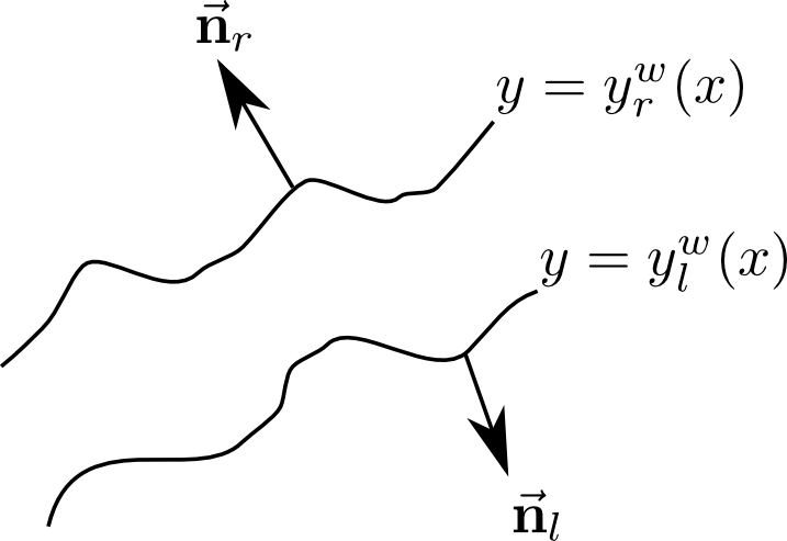
(b) Top view of Lateral Boundaries (at elevation, z=zbw(x)𝑧superscriptsubscript𝑧𝑏𝑤𝑥z=z_{b}^{w}(x)
Figure 3: Non-full channel cross section (left) and channel top view (right).

Let 𝒏l=(nlx,nly)Tsubscript𝒏𝑙superscriptsuperscriptsubscript𝑛𝑙𝑥superscriptsubscript𝑛𝑙𝑦𝑇\vec{\boldsymbol{n}}_{l}=(n_{l}^{x},n_{l}^{y})^{T} and 𝒏r=(nrx,nry)Tsubscript𝒏𝑟superscriptsuperscriptsubscript𝑛𝑟𝑥superscriptsubscript𝑛𝑟𝑦𝑇\vec{\boldsymbol{n}}_{r}=(n_{r}^{x},n_{r}^{y})^{T} be the outward unit normal vectors to the lateral boundaries at y=ylw(x)𝑦subscriptsuperscript𝑦𝑤𝑙𝑥y=y^{w}_{l}(x) and y=yrw(x)𝑦superscriptsubscript𝑦𝑟𝑤𝑥y=y_{r}^{w}(x) respectively (see figure 3(b)). Since these normal vectors are perpendicular to the tangent lines to their respective lateral boundaries, we have

nlynlxxylw(x)=1,nrynrxxyrw(x)=1xylw(x)=nlxnly,xyrw(x)=nrxnry,nly,nry0.formulae-sequencesuperscriptsubscript𝑛𝑙𝑦superscriptsubscript𝑛𝑙𝑥subscript𝑥superscriptsubscript𝑦𝑙𝑤𝑥1formulae-sequencesuperscriptsubscript𝑛𝑟𝑦superscriptsubscript𝑛𝑟𝑥subscript𝑥superscriptsubscript𝑦𝑟𝑤𝑥1formulae-sequencesubscript𝑥superscriptsubscript𝑦𝑙𝑤𝑥superscriptsubscript𝑛𝑙𝑥superscriptsubscript𝑛𝑙𝑦formulae-sequencesubscript𝑥superscriptsubscript𝑦𝑟𝑤𝑥superscriptsubscript𝑛𝑟𝑥superscriptsubscript𝑛𝑟𝑦superscriptsubscript𝑛𝑙𝑦superscriptsubscript𝑛𝑟𝑦0\displaystyle\frac{n_{l}^{y}}{n_{l}^{x}}\partial_{x}y_{l}^{w}(x)=-1,\quad\frac{n_{r}^{y}}{n_{r}^{x}}\partial_{x}y_{r}^{w}(x)=-1\quad\Longrightarrow\quad\partial_{x}y_{l}^{w}(x)=-\frac{n_{l}^{x}}{n_{l}^{y}},\quad\partial_{x}y_{r}^{w}(x)=-\frac{n_{r}^{x}}{n_{r}^{y}},\quad n_{l}^{y},n_{r}^{y}\neq 0.

Define the vector 𝒒=(qx,qy)T𝒒superscriptsubscript𝑞𝑥subscript𝑞𝑦𝑇\vec{\boldsymbol{q}}=(q_{x},q_{y})^{T}, then we write the coupling terms as

ΦA(x,t)=ΦLA(x,t)+ΦRA(x,t) and ΦQ(x,t)=ΦLQ(x,t)+ΦRQ(x,t).formulae-sequencesuperscriptΦ𝐴𝑥𝑡superscriptsubscriptΦ𝐿𝐴𝑥𝑡superscriptsubscriptΦ𝑅𝐴𝑥𝑡 and superscriptΦ𝑄𝑥𝑡superscriptsubscriptΦ𝐿𝑄𝑥𝑡superscriptsubscriptΦ𝑅𝑄𝑥𝑡\Phi^{A}(x,t)=\Phi_{L}^{A}(x,t)+\Phi_{R}^{A}(x,t)\quad\mbox{ and }\quad\Phi^{Q}(x,t)=\Phi_{L}^{Q}(x,t)+\Phi_{R}^{Q}(x,t). (34)

where

ΦLA(x,t)=1nly(𝒒.𝒏l)|y=ylw(x),ΦRA(x,t)=1nry(𝒒.𝒏r)|y=yrw(x),\displaystyle\Phi_{L}^{A}(x,t)=\frac{1}{n_{l}^{y}}\bigg{(}\vec{\boldsymbol{q}}.\vec{\boldsymbol{n}}_{l}\bigg{)}\bigg{|}_{y=y_{l}^{w}(x)},\quad\Phi_{R}^{A}(x,t)=-\frac{1}{n_{r}^{y}}\bigg{(}\vec{\boldsymbol{q}}.\vec{\boldsymbol{n}}_{r}\bigg{)}\bigg{|}_{y=y_{r}^{w}(x)}, (35)
ΦLQ(x,t)=1nly(nlx[qx2(𝑿,t)H(𝑿,t)+g2H2(𝑿,t)]+nlyqy(𝑿,t)qy(𝑿,t)H(𝑿,t))|y=ylw(x)nlxnlyg2H2(𝑿,t)|y=ylw(x),superscriptsubscriptΦ𝐿𝑄𝑥𝑡evaluated-at1superscriptsubscript𝑛𝑙𝑦superscriptsubscript𝑛𝑙𝑥delimited-[]superscriptsubscript𝑞𝑥2𝑿𝑡𝐻𝑿𝑡𝑔2superscript𝐻2𝑿𝑡superscriptsubscript𝑛𝑙𝑦subscript𝑞𝑦𝑿𝑡subscript𝑞𝑦𝑿𝑡𝐻𝑿𝑡𝑦superscriptsubscript𝑦𝑙𝑤𝑥evaluated-atsuperscriptsubscript𝑛𝑙𝑥superscriptsubscript𝑛𝑙𝑦𝑔2superscript𝐻2𝑿𝑡𝑦superscriptsubscript𝑦𝑙𝑤𝑥\displaystyle\Phi_{L}^{Q}(x,t)=\frac{1}{n_{l}^{y}}\bigg{(}n_{l}^{x}\bigg{[}\frac{q_{x}^{2}(\vec{\boldsymbol{X}},t)}{H(\vec{\boldsymbol{X}},t)}+\frac{g}{2}H^{2}(\vec{\boldsymbol{X}},t)\bigg{]}+n_{l}^{y}\frac{q_{y}(\vec{\boldsymbol{X}},t)q_{y}(\vec{\boldsymbol{X}},t)}{H(\vec{\boldsymbol{X}},t)}\bigg{)}\bigg{|}_{y=y_{l}^{w}(x)}-\frac{n_{l}^{x}}{n_{l}^{y}}\frac{g}{2}H^{2}(\vec{\boldsymbol{X}},t)\bigg{|}_{y=y_{l}^{w}(x)}, (36)
ΦRQ(x,t)=1nry(nrx[qx2(𝑿,t)H(𝑿,t)+g2H2(𝑿,t)]+nryqy(𝑿,t)qy(𝑿,t)H(𝑿,t))|y=yrw(x)+nrxnryg2H2(𝑿,t)|y=yrw(x).superscriptsubscriptΦ𝑅𝑄𝑥𝑡evaluated-at1superscriptsubscript𝑛𝑟𝑦superscriptsubscript𝑛𝑟𝑥delimited-[]superscriptsubscript𝑞𝑥2𝑿𝑡𝐻𝑿𝑡𝑔2superscript𝐻2𝑿𝑡superscriptsubscript𝑛𝑟𝑦subscript𝑞𝑦𝑿𝑡subscript𝑞𝑦𝑿𝑡𝐻𝑿𝑡𝑦superscriptsubscript𝑦𝑟𝑤𝑥evaluated-atsuperscriptsubscript𝑛𝑟𝑥superscriptsubscript𝑛𝑟𝑦𝑔2superscript𝐻2𝑿𝑡𝑦superscriptsubscript𝑦𝑟𝑤𝑥\displaystyle\Phi_{R}^{Q}(x,t)=-\frac{1}{n_{r}^{y}}\bigg{(}n_{r}^{x}\bigg{[}\frac{q_{x}^{2}(\vec{\boldsymbol{X}},t)}{H(\vec{\boldsymbol{X}},t)}+\frac{g}{2}H^{2}(\vec{\boldsymbol{X}},t)\bigg{]}+n_{r}^{y}\frac{q_{y}(\vec{\boldsymbol{X}},t)q_{y}(\vec{\boldsymbol{X}},t)}{H(\vec{\boldsymbol{X}},t)}\bigg{)}\bigg{|}_{y=y_{r}^{w}(x)}+\frac{n_{r}^{x}}{n_{r}^{y}}\frac{g}{2}H^{2}(\vec{\boldsymbol{X}},t)\bigg{|}_{y=y_{r}^{w}(x)}. (37)

Let fL1(x,t)subscriptsuperscript𝑓1𝐿𝑥𝑡f^{1}_{L}(x,t) and fL2(x,t)subscriptsuperscript𝑓2𝐿𝑥𝑡f^{2}_{L}(x,t) denote the first and second components, respectively, of the outgoing flux in the direction of 𝒏lsubscript𝒏𝑙\vec{\boldsymbol{n}}_{l} at y=ylw(x)𝑦superscriptsubscript𝑦𝑙𝑤𝑥y=y_{l}^{w}(x), and fR1(x,t)subscriptsuperscript𝑓1𝑅𝑥𝑡f^{1}_{R}(x,t) and fR2(x,t)subscriptsuperscript𝑓2𝑅𝑥𝑡f^{2}_{R}(x,t) be those in the direction of 𝒏rsubscript𝒏𝑟\vec{\boldsymbol{n}}_{r}, then the coupling terms (35)-(37) can be written in the flowing forms:

ΦLA(x,t)=1nlyfL1(x,t).ΦRA(x,t)=1nryfR1(x,t).\displaystyle\Phi_{L}^{A}(x,t)=\frac{1}{n_{l}^{y}}f^{1}_{L}(x,t).\quad\Phi_{R}^{A}(x,t)=-\frac{1}{n_{r}^{y}}f^{1}_{R}(x,t). (38)
ΦLQ(x,t)=1nlyfL2(x,t)nlxnlyg2H2(𝑿,t)|y=ylw(x),superscriptsubscriptΦ𝐿𝑄𝑥𝑡1superscriptsubscript𝑛𝑙𝑦subscriptsuperscript𝑓2𝐿𝑥𝑡evaluated-atsuperscriptsubscript𝑛𝑙𝑥superscriptsubscript𝑛𝑙𝑦𝑔2superscript𝐻2𝑿𝑡𝑦superscriptsubscript𝑦𝑙𝑤𝑥\displaystyle\Phi_{L}^{Q}(x,t)=\frac{1}{n_{l}^{y}}f^{2}_{L}(x,t)-\frac{n_{l}^{x}}{n_{l}^{y}}\frac{g}{2}H^{2}(\vec{\boldsymbol{X}},t)\bigg{|}_{y=y_{l}^{w}(x)},\quad ΦRQ(x,t)=1nryfR2(x,t)+nrxnryg2H2(𝑿,t)|y=yrw(x).superscriptsubscriptΦ𝑅𝑄𝑥𝑡1superscriptsubscript𝑛𝑟𝑦subscriptsuperscript𝑓2𝑅𝑥𝑡evaluated-atsuperscriptsubscript𝑛𝑟𝑥superscriptsubscript𝑛𝑟𝑦𝑔2superscript𝐻2𝑿𝑡𝑦superscriptsubscript𝑦𝑟𝑤𝑥\displaystyle\Phi_{R}^{Q}(x,t)=-\frac{1}{n_{r}^{y}}f^{2}_{R}(x,t)+\frac{n_{r}^{x}}{n_{r}^{y}}\frac{g}{2}H^{2}(\vec{\boldsymbol{X}},t)\bigg{|}_{y=y_{r}^{w}(x)}. (39)

Hence, the 1D channel models with coupling term, in the presence of friction is

tA(x,t)+xQ(x,t)=1nlyfL1(x,t)1nryfR1(x,t),subscript𝑡𝐴𝑥𝑡subscript𝑥𝑄𝑥𝑡1superscriptsubscript𝑛𝑙𝑦subscriptsuperscript𝑓1𝐿𝑥𝑡1superscriptsubscript𝑛𝑟𝑦subscriptsuperscript𝑓1𝑅𝑥𝑡\displaystyle\begin{split}\partial_{t}A(x,t)+\partial_{x}Q(x,t)=&\frac{1}{n_{l}^{y}}f^{1}_{L}(x,t)-\frac{1}{n_{r}^{y}}f^{1}_{R}(x,t),\end{split} (40)
tQ(x,t)+x(Q2(x,t)A(x,t))=gA(x,t)xη¯(x,t)+1nlyfL2(x,t)nlxnlyg2H2(𝑿,t)|y=ylw(x)1nryfR2(x,t)+nrxnryg2H2(𝑿,t)|y=yrw(x)+gA(x,t)Sf.subscript𝑡𝑄𝑥𝑡subscript𝑥superscript𝑄2𝑥𝑡𝐴𝑥𝑡𝑔𝐴𝑥𝑡subscript𝑥¯𝜂𝑥𝑡1superscriptsubscript𝑛𝑙𝑦subscriptsuperscript𝑓2𝐿𝑥𝑡evaluated-atsuperscriptsubscript𝑛𝑙𝑥superscriptsubscript𝑛𝑙𝑦𝑔2superscript𝐻2𝑿𝑡𝑦superscriptsubscript𝑦𝑙𝑤𝑥1superscriptsubscript𝑛𝑟𝑦subscriptsuperscript𝑓2𝑅𝑥𝑡evaluated-atsuperscriptsubscript𝑛𝑟𝑥superscriptsubscript𝑛𝑟𝑦𝑔2superscript𝐻2𝑿𝑡𝑦superscriptsubscript𝑦𝑟𝑤𝑥𝑔𝐴𝑥𝑡subscript𝑆𝑓\displaystyle\begin{split}\partial_{t}Q(x,t)+\partial_{x}\left(\frac{Q^{2}(x,t)}{A(x,t)}\right)=&-gA(x,t)\partial_{x}\bar{\eta}(x,t)+\frac{1}{n_{l}^{y}}f^{2}_{L}(x,t)-\frac{n_{l}^{x}}{n_{l}^{y}}\frac{g}{2}H^{2}(\vec{\boldsymbol{X}},t)\bigg{|}_{y=y_{l}^{w}(x)}\\ &-\frac{1}{n_{r}^{y}}f^{2}_{R}(x,t)+\frac{n_{r}^{x}}{n_{r}^{y}}\frac{g}{2}H^{2}(\vec{\boldsymbol{X}},t)\bigg{|}_{y=y_{r}^{w}(x)}+gA(x,t)S_{f}.\end{split} (41)

where Sf=Q|Q|K2subscript𝑆𝑓𝑄𝑄superscript𝐾2S_{f}=\frac{Q|Q|}{K^{2}} is the channel friction slope, K=Ak1nPk2𝐾superscript𝐴subscript𝑘1𝑛superscript𝑃subscript𝑘2K=\frac{A^{k_{1}}}{nP^{k_{2}}} is the conveyance, P𝑃P is the wetted perimeter of channel cross-section, k1=5/3,k2=2/3formulae-sequencesubscript𝑘153subscript𝑘223k_{1}=5/3,k_{2}=2/3 and n𝑛n is the Manning coefficient, see [5, 11].

Remark 2.1

We obtained the above coupling terms without using or imposing any restriction on the channel width variation as done in [12]. And our coupling term clearly differs from theirs.

2.2.1 Channel Flow Lateral Discharge Model

To compute the lateral discharges in the channel, we use the following y𝑦y-discharge equation in the 2D Shallow water equations :

tqy(𝑿,t)+xfx(Π)+yfy(Π)=gH(𝑿,t)yzb(𝑿),Π=(H,qx,qy)T,fx(Π)=qxqyH,fy(Π)=qy2H+12gH2.\begin{split}\partial_{t}q_{y}(\vec{\boldsymbol{X}},t)+\partial_{x}f_{x}(\Pi)+\partial_{y}f_{y}(\Pi)=-gH(\vec{\boldsymbol{X}},t)\partial_{y}z_{b}(\vec{\boldsymbol{X}}),\\ \Pi=(H,q_{x},q_{y})^{T},\quad f_{x}(\Pi)=\frac{q_{x}q_{y}}{H},\quad f_{y}(\Pi)=\frac{q_{y}^{2}}{H}+\frac{1}{2}gH^{2}.\end{split} (42)

2.3 Floodplain Flow Model

We describe the flow in the floodplains using the 2D Shallow water equations, namely

tΠ+F(Π)=S(Π,zb)+Sb(Π),subscript𝑡Π𝐹Π𝑆Πsubscript𝑧𝑏subscript𝑆𝑏Π\displaystyle\partial_{t}\Pi+\nabla\cdot F(\Pi)=S(\Pi,z_{b})+S_{b}(\Pi), (43)

where

Π=(Hqxqy),F(Π)=(F1(Π),F2(Π)),F1(Π)=(qxqx2H+12gH2qxqyH),F2(Π)=(qyqxqyHqy2H+12gH2),Sb(Π)=(0gn2H7/3q|q|),S(Π,zb)=(0gHxzb(𝑿)ghyzb(𝑿)),\displaystyle\begin{split}&\Pi=\begin{pmatrix}H\\ q_{x}\\ q_{y}\end{pmatrix},\quad F(\Pi)=\bigg{(}F_{1}(\Pi),F_{2}(\Pi)\bigg{)},\quad F_{1}(\Pi)=\begin{pmatrix}q_{x}\\ \frac{q_{x}^{2}}{H}+\frac{1}{2}gH^{2}\\ \frac{q_{x}q_{y}}{H}\end{pmatrix},\quad F_{2}(\Pi)=\begin{pmatrix}q_{y}\\ \frac{q_{x}q_{y}}{H}\\ \frac{q_{y}^{2}}{H}+\frac{1}{2}gH^{2}\end{pmatrix},\\ &S_{b}(\Pi)=\begin{pmatrix}0\\ -g\frac{n^{2}}{H^{7/3}}\vec{q}|\vec{q}|\end{pmatrix},\quad S(\Pi,z_{b})=\begin{pmatrix}0\\ -gH\partial_{x}z_{b}(\vec{\boldsymbol{X}})\\ -gh\partial_{y}z_{b}(\vec{\boldsymbol{X}})\end{pmatrix},\end{split} (44)

where n𝑛n is the manning coefficient, Sbsubscript𝑆𝑏S_{b} is the friction term and S(Π,zb)𝑆Πsubscript𝑧𝑏S(\Pi,z_{b}) is the source term due to bottom topography term.

3 Numerical Schemes

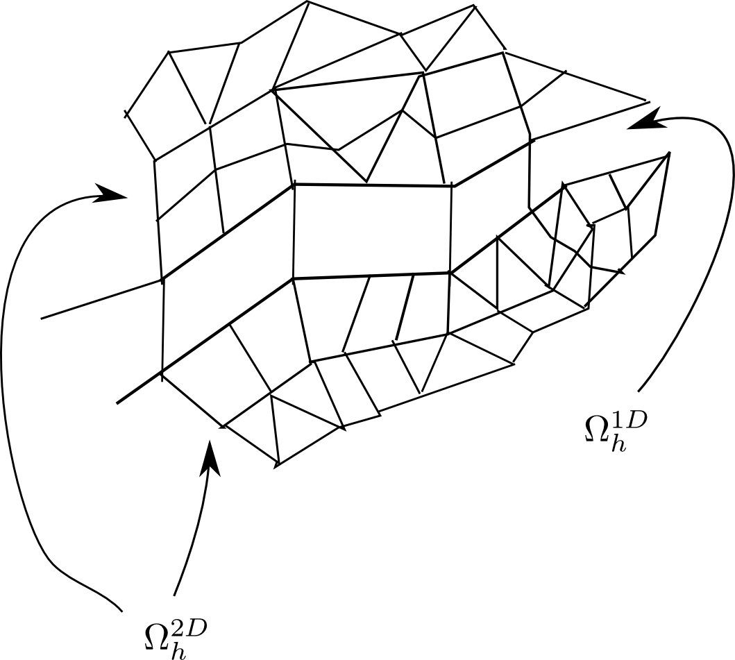
In this section, we detail the numerical schemes for the models presented in previous sections. To begin, we partition the channel into a 1D grid, Ωh1DsuperscriptsubscriptΩ1𝐷\Omega_{h}^{1D} made of cross sections and the floodplains, into a 2D grid Ωh2DsuperscriptsubscriptΩ2𝐷\Omega_{h}^{2D}, see figure 4(a). We first present the scheme for the 2D flood model, then the schemes for the channel flow model is presented.
Refer to caption
(a) Grid of the entire domain consisting of the 1D grid Ωh1DsuperscriptsubscriptΩ1𝐷\Omega_{h}^{1D} at the middle and the 2D grids Ωh2DsuperscriptsubscriptΩ2𝐷\Omega_{h}^{2D} for the floodplains.
Refer to caption
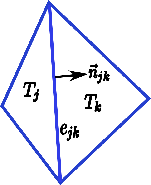
(b) 2D mesh showing two neighbour cells, Tjsubscript𝑇𝑗T_{j} and Tksubscript𝑇𝑘T_{k}, the edge ejksubscript𝑒𝑗𝑘e_{jk} between them and the normal vector njksubscript𝑛𝑗𝑘\vec{n}_{jk}.
Figure 4: Grids

3.1 Scheme For 2D Model

In this section, we present the scheme for the flood flow model, (43). Let TjΩh2Dsubscript𝑇𝑗superscriptsubscriptΩ2𝐷T_{j}\in\Omega_{h}^{2D} be an element of the 2D mesh Ωh2DsuperscriptsubscriptΩ2𝐷\Omega_{h}^{2D} in figure 4(a), and TkΩh2Dsubscript𝑇𝑘superscriptsubscriptΩ2𝐷T_{k}\in\Omega_{h}^{2D} be its neighbour cell, see figure 4(b). Let ejksubscript𝑒𝑗𝑘e_{jk} be the edge between Tjsubscript𝑇𝑗T_{j} and Tksubscript𝑇𝑘T_{k}, while njksubscript𝑛𝑗𝑘\vec{n}_{jk} is a unit vector normal to edge ejksubscript𝑒𝑗𝑘e_{jk} and outward to Tjsubscript𝑇𝑗T_{j}. Furthermore, let |Tj|subscript𝑇𝑗|T_{j}| and |ejk|subscript𝑒𝑗𝑘|e_{jk}| be the area of Tjsubscript𝑇𝑗T_{j} and length of ejksubscript𝑒𝑗𝑘e_{jk} respectively and let jsubscript𝑗\mathcal{E}_{j} be the set of all edges of Tjsubscript𝑇𝑗T_{j}. And let Πjn=(Hjn,qx,jn,qy,jn)TsuperscriptsubscriptΠ𝑗𝑛superscriptsuperscriptsubscript𝐻𝑗𝑛superscriptsubscript𝑞𝑥𝑗𝑛superscriptsubscript𝑞𝑦𝑗𝑛𝑇\Pi_{j}^{n}=(H_{j}^{n},q_{x,j}^{n},q_{y,j}^{n})^{T} be the approximate cell averages of the true solution in Tjsubscript𝑇𝑗T_{j}, namely

Πjn=1|Tj|TjΠ(𝑿,tn)𝑑x.superscriptsubscriptΠ𝑗𝑛1subscript𝑇𝑗subscriptsubscript𝑇𝑗Π𝑿superscript𝑡𝑛differential-d𝑥\displaystyle\Pi_{j}^{n}=\frac{1}{|T_{j}|}\int_{T_{j}}\Pi(\vec{\boldsymbol{X}},t^{n})d\vec{x}. (45)

Similarly, let Πkn=(Hkn,qx,kn,qy,kn)TsuperscriptsubscriptΠ𝑘𝑛superscriptsuperscriptsubscript𝐻𝑘𝑛superscriptsubscript𝑞𝑥𝑘𝑛superscriptsubscript𝑞𝑦𝑘𝑛𝑇\Pi_{k}^{n}=(H_{k}^{n},q_{x,k}^{n},q_{y,k}^{n})^{T} be the cell average vector Tksubscript𝑇𝑘T_{k}, while zb,j,zb,ksubscript𝑧𝑏𝑗subscript𝑧𝑏𝑘z_{b,j},z_{b,k} are the cell averages in Tj,Tksubscript𝑇𝑗subscript𝑇𝑘T_{j},T_{k} respectively.

Then, we consider the following 2D hydrostatic reconstruction finite volume scheme [1]:

Πjn+1=ΠjnΔt|Tj|ejkj|ejk|(Tnjk1ϕ(TnjkΠjn~,TnjkΠkn~)+Tnjk1Shrm(Hjn,H~jn))+ΔtSb(Πjn),superscriptsubscriptΠ𝑗𝑛1superscriptsubscriptΠ𝑗𝑛Δ𝑡subscript𝑇𝑗subscriptsubscript𝑒𝑗𝑘subscript𝑗subscript𝑒𝑗𝑘superscriptsubscript𝑇subscript𝑛𝑗𝑘1italic-ϕ~subscript𝑇subscript𝑛𝑗𝑘superscriptsubscriptΠ𝑗𝑛~subscript𝑇subscript𝑛𝑗𝑘superscriptsubscriptΠ𝑘𝑛superscriptsubscript𝑇subscript𝑛𝑗𝑘1superscript𝑆𝑟𝑚superscriptsubscript𝐻𝑗𝑛superscriptsubscript~𝐻𝑗𝑛Δ𝑡subscript𝑆𝑏superscriptsubscriptΠ𝑗𝑛\displaystyle\begin{split}\Pi_{j}^{n+1}=&\Pi_{j}^{n}-\frac{\Delta t}{|T_{j}|}\sum_{e_{jk}\in\mathcal{E}_{j}}|e_{jk}|\bigg{(}T_{\vec{n}_{jk}}^{-1}\phi(\widetilde{T_{\vec{n}_{jk}}\Pi_{j}^{n}},\widetilde{T_{\vec{n}_{jk}}\Pi_{k}^{n}})+T_{\vec{n}_{jk}}^{-1}S^{hrm}(H_{j}^{n},\tilde{H}_{j}^{n})\bigg{)}\\ &+\Delta tS_{b}(\Pi_{j}^{n}),\end{split} (46)

where

H~pn:=max(Hpn+zb,pmax(zb,j,zb,k)),TnjkΠpn~:=H~pnHpnTnjkΠpn,p=j,k.formulae-sequenceassignsuperscriptsubscript~𝐻𝑝𝑛superscriptsubscript𝐻𝑝𝑛subscript𝑧𝑏𝑝subscript𝑧𝑏𝑗subscript𝑧𝑏𝑘formulae-sequenceassign~subscript𝑇subscript𝑛𝑗𝑘superscriptsubscriptΠ𝑝𝑛subscriptsuperscript~𝐻𝑛𝑝superscriptsubscript𝐻𝑝𝑛subscript𝑇subscript𝑛𝑗𝑘superscriptsubscriptΠ𝑝𝑛𝑝𝑗𝑘\displaystyle\tilde{H}_{p}^{n}:=\max(H_{p}^{n}+z_{b,p}-\max(z_{b,j},z_{b,k})),\quad\widetilde{T_{\vec{n}_{jk}}\Pi_{p}^{n}}:=\frac{\tilde{H}^{n}_{p}}{H_{p}^{n}}T_{\vec{n}_{jk}}\Pi_{p}^{n},\quad p=j,k. (47)
Shrm(Hjn,H~jn):=(0g2((Hjn)2(H~jn)2)0).assignsuperscript𝑆𝑟𝑚superscriptsubscript𝐻𝑗𝑛superscriptsubscript~𝐻𝑗𝑛matrix0𝑔2superscriptsuperscriptsubscript𝐻𝑗𝑛2superscriptsuperscriptsubscript~𝐻𝑗𝑛20\displaystyle S^{hrm}(H_{j}^{n},\tilde{H}_{j}^{n}):=\begin{pmatrix}0\\ \frac{g}{2}((H_{j}^{n})^{2}-(\tilde{H}_{j}^{n})^{2})\\ 0\end{pmatrix}. (48)

The function,ϕitalic-ϕ\phi is any numerical flux function consistent with the 1D component, F1(Π)subscript𝐹1ΠF_{1}(\Pi) of the 2D flux, F(Π)𝐹ΠF(\Pi). Here, we consider the HLL scheme [9], namely

ϕ(ΠL,ΠR)={F1(ΠL), if sL0,F1:=sRF1(ΠL)sLF1(ΠR)+sLsR(ΠRΠL)sRsL, if sL0sR,F1(ΠR), if sR0,italic-ϕsubscriptΠ𝐿subscriptΠ𝑅casessubscript𝐹1subscriptΠ𝐿 if subscript𝑠𝐿0assignsuperscriptsubscript𝐹1subscript𝑠𝑅subscript𝐹1subscriptΠ𝐿subscript𝑠𝐿subscript𝐹1subscriptΠ𝑅subscript𝑠𝐿subscript𝑠𝑅subscriptΠ𝑅subscriptΠ𝐿subscript𝑠𝑅subscript𝑠𝐿 if subscript𝑠𝐿0subscript𝑠𝑅subscript𝐹1subscriptΠ𝑅 if subscript𝑠𝑅0\displaystyle\phi(\Pi_{L},\Pi_{R})=\begin{cases}F_{1}(\Pi_{L}),&\mbox{ if }s_{L}\geq 0,\\ F_{1}^{*}:=\frac{s_{R}F_{1}(\Pi_{L})-s_{L}F_{1}(\Pi_{R})+s_{L}s_{R}(\Pi_{R}-\Pi_{L})}{s_{R}-s_{L}},&\mbox{ if }s_{L}\leq 0\leq s_{R},\\ F_{1}(\Pi_{R}),&\mbox{ if }s_{R}\leq 0,\end{cases} (49)

where sLsubscript𝑠𝐿s_{L} and sRsubscript𝑠𝑅s_{R} are estimates of the smallest and largest wave speeds in the solution of the associated 1D Riemann problem [20]. There are several choices for sL,sRsubscript𝑠𝐿subscript𝑠𝑅s_{L},s_{R} [20, 19]. We use the ones given in [3] namely

sL=mink{λk(ΠL),λk(ΠR)},sR=maxk{λk(ΠL),λk(ΠR)},formulae-sequencesubscript𝑠𝐿subscript𝑘subscript𝜆𝑘subscriptΠ𝐿subscript𝜆𝑘subscriptΠ𝑅subscript𝑠𝑅subscript𝑘subscript𝜆𝑘subscriptΠ𝐿subscript𝜆𝑘subscriptΠ𝑅\displaystyle s_{L}=\min_{k}\{\lambda_{k}(\Pi_{L}),\lambda_{k}(\Pi_{R})\},\quad s_{R}=\max_{k}\{\lambda_{k}(\Pi_{L}),\lambda_{k}(\Pi_{R})\}, (50)

where λk,k=1,,Mformulae-sequencesubscript𝜆𝑘𝑘1𝑀\lambda_{k},k=1,...,M , are the eigenvalues of the Jacobian matrix of the system.

And Tnsubscript𝑇𝑛T_{\vec{n}} is a rotation matrix which depends on the normal vector, n=(nx,ny)T𝑛superscriptsubscript𝑛𝑥subscript𝑛𝑦𝑇\vec{n}=(n_{x},n_{y})^{T} and Tn1superscriptsubscript𝑇𝑛1T_{\vec{n}}^{-1} is its inverse; they are given by

Tn=(1000nxny0nynx),Tn1=(1000nxny0nynx),formulae-sequencesubscript𝑇𝑛matrix1000subscript𝑛𝑥subscript𝑛𝑦0subscript𝑛𝑦subscript𝑛𝑥superscriptsubscript𝑇𝑛1matrix1000subscript𝑛𝑥subscript𝑛𝑦0subscript𝑛𝑦subscript𝑛𝑥\displaystyle T_{\vec{n}}=\begin{pmatrix}1&0&0\\ 0&n_{x}&n_{y}\\ 0&-n_{y}&n_{x}\end{pmatrix},\quad T_{\vec{n}}^{-1}=\begin{pmatrix}1&0&0\\ 0&n_{x}&-n_{y}\\ 0&n_{y}&n_{x}\end{pmatrix}, (51)

see [20].

3.2 Schemes for the Channel Models

Here, we describe the finite volume method to discretize the channel models with coupling terms, equations (40), (41) and (42). To design a method which reuses existing 1D channel solvers, we discretize the purely 1D channel models, (40) and (41) separately from the lateral discharge model, (42). Let {xi+1/2}i=1N1Dcellsuperscriptsubscriptsubscript𝑥𝑖12𝑖1subscript𝑁1𝐷𝑐𝑒𝑙𝑙\{x_{i+1/2}\}_{i=1}^{N_{1Dcell}} be points in the 1D grid, Ωh1DsuperscriptsubscriptΩ1𝐷\Omega_{h}^{1D} and Ki=(xi1/2,xi+1/2),i=1,2,..,N1DcellK_{i}=(x_{i-1/2},x_{i+1/2}),i=1,2,..,N_{1Dcell} be a cell centred at xi=(xi1/2+xi+1/2)/2subscript𝑥𝑖subscript𝑥𝑖12subscript𝑥𝑖122x_{i}=(x_{i-1/2}+x_{i+1/2})/2 in Ωh1DsuperscriptsubscriptΩ1𝐷\Omega_{h}^{1D} . Where N1Dcellsubscript𝑁1𝐷𝑐𝑒𝑙𝑙N_{1Dcell} is the number of cells in the 1D grid. Let 𝑾(x,t)=(A(x,t),Q(x,t))T𝑾𝑥𝑡superscript𝐴𝑥𝑡𝑄𝑥𝑡𝑇\boldsymbol{W}(x,t)=(A(x,t),Q(x,t))^{T} be a vector of conserved quantities at point, x𝑥x and time, t𝑡t, then the cell average vector, 𝑾in=(Ain,Qin)Tsuperscriptsubscript𝑾𝑖𝑛superscriptsuperscriptsubscript𝐴𝑖𝑛superscriptsubscript𝑄𝑖𝑛𝑇\boldsymbol{W}_{i}^{n}=(A_{i}^{n},Q_{i}^{n})^{T} in cell Kisubscript𝐾𝑖K_{i} is defined as

𝑾in:=1ΔxiKi𝑾(x,tn)𝑑xassignsubscriptsuperscript𝑾𝑛𝑖1Δsubscript𝑥𝑖subscriptsubscript𝐾𝑖𝑾𝑥superscript𝑡𝑛differential-d𝑥\boldsymbol{W}^{n}_{i}:=\frac{1}{\Delta x_{i}}\int_{K_{i}}\boldsymbol{W}(x,t^{n})dx (52)

where Δxi=xi+1/2xi1/2,tn=tn1+Δtformulae-sequenceΔsubscript𝑥𝑖subscript𝑥𝑖12subscript𝑥𝑖12superscript𝑡𝑛superscript𝑡𝑛1Δ𝑡\Delta x_{i}=x_{i+1/2}-x_{i-1/2},t^{n}=t^{n-1}+\Delta t, and ΔtΔ𝑡\Delta t is the time step.

Refer to caption
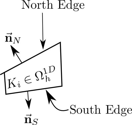
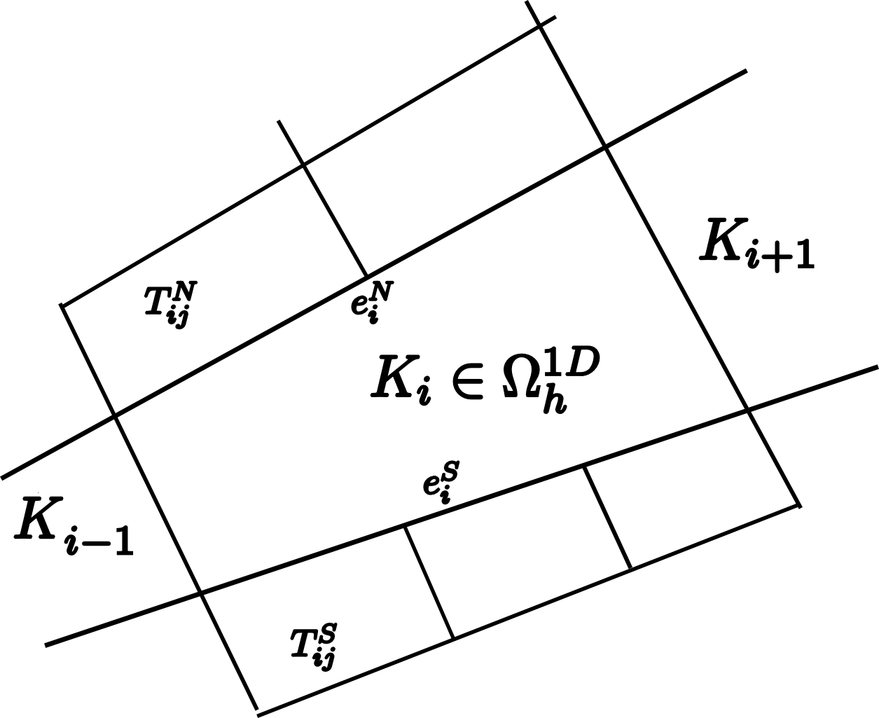
Figure 5: A single cell, Kisubscript𝐾𝑖K_{i} in the 1D channel mesh showing its lateral edges; South edge eiSsuperscriptsubscript𝑒𝑖𝑆e_{i}^{S} is on the negative y𝑦y-direction while the North edge eiNsuperscriptsubscript𝑒𝑖𝑁e_{i}^{N} is on the positive y𝑦y-direction. These edges are the interfaces between the 1D cell and the adjacent 2D floodplain cells.

For each 1D cell, KiΩh1Dsubscript𝐾𝑖superscriptsubscriptΩ1𝐷K_{i}\in\Omega_{h}^{1D}, the channel lateral boundaries, y=ylw(x)𝑦superscriptsubscript𝑦𝑙𝑤𝑥y=y_{l}^{w}(x) and y=yrw(x)𝑦superscriptsubscript𝑦𝑟𝑤𝑥y=y_{r}^{w}(x) are approximated with straight edges which we call South (S) and North (N) edges (or faces) respectively with unit normals 𝒏S=(nSx,nSy)Tsubscript𝒏𝑆superscriptsuperscriptsubscript𝑛𝑆𝑥superscriptsubscript𝑛𝑆𝑦𝑇\vec{\boldsymbol{n}}_{S}=(n_{S}^{x},n_{S}^{y})^{T} and 𝒏N=(nNx,nNy)Tsubscript𝒏𝑁superscriptsuperscriptsubscript𝑛𝑁𝑥superscriptsubscript𝑛𝑁𝑦𝑇\vec{\boldsymbol{n}}_{N}=(n_{N}^{x},n_{N}^{y})^{T} (see figure 5). This means that the channel normals, 𝒏lsubscript𝒏𝑙\vec{\boldsymbol{n}}_{l} and 𝒏rsubscript𝒏𝑟\vec{\boldsymbol{n}}_{r} are approximated with the edge normals 𝒏Ssubscript𝒏𝑆\vec{\boldsymbol{n}}_{S} and 𝒏Nsubscript𝒏𝑁\vec{\boldsymbol{n}}_{N} respectively, that is

𝒏l𝒏S,𝒏r𝒏N.formulae-sequencesubscript𝒏𝑙subscript𝒏𝑆subscript𝒏𝑟subscript𝒏𝑁\vec{\boldsymbol{n}}_{l}\approx\vec{\boldsymbol{n}}_{S},\quad\vec{\boldsymbol{n}}_{r}\approx\vec{\boldsymbol{n}}_{N}. (53)

We start by presenting the scheme of the 1D model without coupling terms, next the scheme for channel lateral discharge model is presented and finally, the discrete coupling term is derived.

3.2.1 Scheme for 1D Model without Coupling Terms

We now focus on the 1D channel model (40)-(41) but without the coupling terms, namely,

tA(x,t)+xQ(x,t)=0.tQ(x,t)+x(Q2(x,t)A(x,t))=gA(x,t)xη¯(x,t)+gA(x,t)Sf.formulae-sequencesubscript𝑡𝐴𝑥𝑡subscript𝑥𝑄𝑥𝑡0subscript𝑡𝑄𝑥𝑡subscript𝑥superscript𝑄2𝑥𝑡𝐴𝑥𝑡𝑔𝐴𝑥𝑡subscript𝑥¯𝜂𝑥𝑡𝑔𝐴𝑥𝑡subscript𝑆𝑓\displaystyle\begin{split}\partial_{t}A(x,t)&+\partial_{x}Q(x,t)=0.\\ \partial_{t}Q(x,t)&+\partial_{x}\bigg{(}\frac{Q^{2}(x,t)}{A(x,t)}\bigg{)}=-gA(x,t)\partial_{x}\bar{\eta}(x,t)+gA(x,t)S_{f}.\end{split} (54)

We consider the scheme of [15] as summarised in [14]. The scheme is based on the formulation of the St Venant model as presented in [5] and rewrites the model in the quasi-linear form.

t𝑾+J(𝑾,B)x𝑾=s(x,𝑾),subscript𝑡𝑾𝐽𝑾𝐵subscript𝑥𝑾superscript𝑠𝑥𝑾\displaystyle\partial_{t}\boldsymbol{W}+J(\boldsymbol{W},B)\partial_{x}\boldsymbol{W}=s^{\prime}(x,\boldsymbol{W}), (55)

where 𝑾=(A,Q)T𝑾superscript𝐴𝑄𝑇\boldsymbol{W}=(A,Q)^{T}, the Jacobian matrix,J𝐽J is given by

J(𝑾,B)=(01c2u¯22u¯),u¯=QA,c=gAB,s(x,𝑾)=(0gA[SoSfdH¯dx+1BdAdx]),formulae-sequence𝐽𝑾𝐵matrix01superscript𝑐2superscript¯𝑢22¯𝑢formulae-sequence¯𝑢𝑄𝐴formulae-sequence𝑐𝑔𝐴𝐵superscript𝑠𝑥𝑾matrix0𝑔𝐴delimited-[]subscript𝑆𝑜subscript𝑆𝑓𝑑¯𝐻𝑑𝑥1𝐵𝑑𝐴𝑑𝑥\displaystyle J(\boldsymbol{W},B)=\begin{pmatrix}0&1\\ c^{2}-\underline{u}^{2}&2\underline{u}\end{pmatrix},\quad\underline{u}=\frac{Q}{A},c=\sqrt{g\frac{A}{B}},\quad s^{\prime}(x,\boldsymbol{W})=\begin{pmatrix}0\\ gA\bigg{[}S_{o}-S_{f}-\frac{d\underline{H}}{dx}+\frac{1}{B}\frac{dA}{dx}\bigg{]}\end{pmatrix}, (56)

B𝐵B is the top width at the free-surface, H¯¯𝐻\underline{H} is the water depth from the 1D bottom elevation, Zb(x)subscript𝑍𝑏𝑥Z_{b}(x) to the flat free-surface, η¯¯𝜂\bar{\eta} and So=dZbdxsubscript𝑆𝑜𝑑subscript𝑍𝑏𝑑𝑥S_{o}=-\frac{dZ_{b}}{dx} is the negative of channel bed slope. Details about this formulation can be found in [14]. The eigenvalues and eigenvectors of J(𝑾,B)𝐽𝑾𝐵J(\boldsymbol{W},B) are

λ1(𝑾,B)=u¯c,λ2(𝑾,B)=u¯+c and e1(𝑾,B)=(1,λ1(𝑾,B))T,e2(𝑾,B)=(1,λ2(𝑾,B))Tformulae-sequenceformulae-sequencesubscript𝜆1𝑾𝐵¯𝑢𝑐subscript𝜆2𝑾𝐵¯𝑢𝑐subscript and e1𝑾𝐵superscript1subscript𝜆1𝑾𝐵𝑇subscripte2𝑾𝐵superscript1subscript𝜆2𝑾𝐵𝑇\displaystyle\lambda_{1}(\boldsymbol{W},B)=\underline{u}-c,\,\lambda_{2}(\boldsymbol{W},B)=\underline{u}+c\mbox{ and }\textbf{e}_{1}(\boldsymbol{W},B)=(1,\lambda_{1}(\boldsymbol{W},B))^{T},\,\textbf{e}_{2}(\boldsymbol{W},B)=(1,\lambda_{2}(\boldsymbol{W},B))^{T}

respectively.

Define the Roe averages:

A^i+1/2=12(Ai+Ai+1)u¯^i+1/2=Aiu¯i+Ai+1u¯i+1Ai+Ai+1,𝑾^i+1/2=(A^i+1/2A^i+1/2u¯^i+1/2).formulae-sequencesubscript^𝐴𝑖1212subscript𝐴𝑖subscript𝐴𝑖1formulae-sequencesubscript^¯𝑢𝑖12subscript𝐴𝑖subscript¯𝑢𝑖subscript𝐴𝑖1subscript¯𝑢𝑖1subscript𝐴𝑖subscript𝐴𝑖1subscript^𝑾𝑖12matrixsubscript^𝐴𝑖12subscript^𝐴𝑖12subscript^¯𝑢𝑖12\displaystyle\hat{A}_{i+1/2}=\frac{1}{2}(A_{i}+A_{i+1})\quad\hat{\underline{u}}_{i+1/2}=\frac{\sqrt{A_{i}}\underline{u}_{i}+\sqrt{A_{i+1}}\underline{u}_{i+1}}{\sqrt{A_{i}}+\sqrt{A_{i+1}}},\quad\hat{\boldsymbol{W}}_{i+1/2}=\begin{pmatrix}\hat{A}_{i+1/2}\\ \hat{A}_{i+1/2}\hat{\underline{u}}_{i+1/2}\end{pmatrix}. (57)
B^i+1/2=12(Bi+Bi+1)H¯^i+1/2=(A^B^)i+1/2,c^i+1/2=gH¯^i+1/2.formulae-sequencesubscript^𝐵𝑖1212subscript𝐵𝑖subscript𝐵𝑖1formulae-sequencesubscript^¯𝐻𝑖12subscript^𝐴^𝐵𝑖12subscript^𝑐𝑖12𝑔subscript^¯𝐻𝑖12\displaystyle\hat{B}_{i+1/2}=\frac{1}{2}(B_{i}+B_{i+1})\quad\hat{\underline{H}}_{i+1/2}=\bigg{(}\frac{\hat{A}}{\hat{B}}\bigg{)}_{i+1/2},\quad\hat{c}_{i+1/2}=\sqrt{g\hat{\underline{H}}_{i+1/2}}. (58)
(So^)i+1/2=Zb,i+1Zb,ixi+1xi,(Sf^)i+1/2=Sf(w^i+1/2).formulae-sequencesubscript^subscript𝑆𝑜𝑖12subscript𝑍𝑏𝑖1subscript𝑍𝑏𝑖subscript𝑥𝑖1subscript𝑥𝑖subscript^subscript𝑆𝑓𝑖12subscript𝑆𝑓subscript^𝑤𝑖12\displaystyle(\hat{S_{o}})_{i+1/2}=\frac{Z_{b,i+1}-Z_{b,i}}{x_{i+1}-x_{i}},\quad(\hat{S_{f}})_{i+1/2}=S_{f}(\hat{w}_{i+1/2}). (59)

Define (Δp)i+1/2=pi+1pisubscriptΔ𝑝𝑖12subscript𝑝𝑖1subscript𝑝𝑖(\Delta p)_{i+1/2}=p_{i+1}-p_{i} for any quantity, p𝑝p. Then, define

(α^1)i+1/2=[λ^2ΔAΔQ2c^]i+/2,(α^2)i+1/2=[λ^1ΔA+ΔQ2c^]i+1/2.formulae-sequencesubscriptsubscript^𝛼1𝑖12subscriptdelimited-[]subscript^𝜆2Δ𝐴Δ𝑄2^𝑐limit-from𝑖absent2subscriptsubscript^𝛼2𝑖12subscriptdelimited-[]subscript^𝜆1Δ𝐴Δ𝑄2^𝑐𝑖12\displaystyle(\hat{\alpha}_{1})_{i+1/2}=\bigg{[}\frac{\hat{\lambda}_{2}\Delta A-\Delta Q}{2\hat{c}}\bigg{]}_{i+/2},\quad(\hat{\alpha}_{2})_{i+1/2}=\bigg{[}\frac{-\hat{\lambda}_{1}\Delta A+\Delta Q}{2\hat{c}}\bigg{]}_{i+1/2}. (60)
(β^1)i+1/2=(gA^2c^[(S^0S^f)ΔxΔH¯+1B^ΔA])i+1/2,(β^2)i+1/2=(β^1)i+1/2.formulae-sequencesubscriptsubscript^𝛽1𝑖12subscript𝑔^𝐴2^𝑐delimited-[]subscript^𝑆0subscript^𝑆𝑓Δ𝑥Δ¯𝐻1^𝐵Δ𝐴𝑖12subscriptsubscript^𝛽2𝑖12subscriptsubscript^𝛽1𝑖12\displaystyle(\hat{\beta}_{1})_{i+1/2}=\bigg{(}-g\frac{\hat{A}}{2\hat{c}}\left[(\hat{S}_{0}-\hat{S}_{f})\Delta x-\Delta\underline{H}+\frac{1}{\hat{B}}\Delta A\right]\bigg{)}_{i+1/2},\quad(\hat{\beta}_{2})_{i+1/2}=-(\hat{\beta}_{1})_{i+1/2}. (61)

The Roe averaged eigenvalues and eigenvectors are

(λ^m)i+1/2:=λm(𝑾^i+2,B^i+1/2),(e^m)i+1/2:=em(𝑾^i+1/2,B^i+1/2),m=1,2.formulae-sequenceassignsubscriptsubscript^𝜆𝑚𝑖12subscript𝜆𝑚subscript^𝑾𝑖2subscript^𝐵𝑖12formulae-sequenceassignsubscriptsubscript^e𝑚𝑖12subscripte𝑚subscript^𝑾𝑖12subscript^𝐵𝑖12𝑚12\displaystyle(\hat{\lambda}_{m})_{i+1/2}:=\lambda_{m}(\hat{\boldsymbol{W}}_{i+2},\hat{B}_{i+1/2}),\quad(\hat{\textbf{e}}_{m})_{i+1/2}:=\textbf{e}_{m}(\hat{\boldsymbol{W}}_{i+1/2},\hat{B}_{i+1/2}),\quad m=1,2. (62)

The artificial viscosity (entropy fix), ν^^𝜈\hat{\nu} to correct the entropy problem associated with the Roe method [14] is given by

(ν^m)i+1/2={14[(λm)i+1(λm)i], if (λm)i<0<(λm)i+10, else ,m=1,2.formulae-sequencesubscriptsubscript^𝜈𝑚𝑖12cases14delimited-[]subscriptsubscript𝜆𝑚𝑖1subscriptsubscript𝜆𝑚𝑖 if subscriptsubscript𝜆𝑚𝑖0subscriptsubscript𝜆𝑚𝑖10 else 𝑚12\displaystyle(\hat{\nu}_{m})_{i+1/2}=\begin{cases}\frac{1}{4}\bigg{[}(\lambda_{m})_{i+1}-(\lambda_{m})_{i}\bigg{]},&\mbox{ if }(\lambda_{m})_{i}<0<(\lambda_{m})_{i+1}\\ 0,&\mbox{ else }\end{cases},\quad m=1,2. (63)

Hence, the numerical scheme of [14, 15] for the 1D channel model without coupling term, (54) is given by

𝑾in+1=𝑾inΔtΔx[m=12(γ^m+e^m)i1/2+m=12(γ^me^m)i+1/2]n,superscriptsubscript𝑾𝑖𝑛1superscriptsubscript𝑾𝑖𝑛Δ𝑡Δ𝑥superscriptdelimited-[]superscriptsubscript𝑚12subscriptsuperscriptsubscript^𝛾𝑚subscript^e𝑚𝑖12superscriptsubscript𝑚12subscriptsuperscriptsubscript^𝛾𝑚subscript^e𝑚𝑖12𝑛\displaystyle\boldsymbol{W}_{i}^{n+1*}=\boldsymbol{W}_{i}^{n}-\frac{\Delta t}{\Delta x}\bigg{[}\sum_{m=1}^{2}\bigg{(}\hat{\gamma}_{m}^{+}\hat{\textbf{e}}_{m}\bigg{)}_{i-1/2}+\sum_{m=1}^{2}\bigg{(}\hat{\gamma}_{m}^{-}\hat{\textbf{e}}_{m}\bigg{)}_{i+1/2}\bigg{]}^{n}, (64)

where

(γ^m±)i+1/2=[12[1±sgn(λ^)]γ^±ν^α^]m,i+1/2,(γ^m)i+1/2=(λ^α^β^)m,i+1/2,m=1,2.formulae-sequencesubscriptsuperscriptsubscript^𝛾𝑚plus-or-minus𝑖12subscriptdelimited-[]plus-or-minus12delimited-[]plus-or-minus1𝑠𝑔𝑛^𝜆^𝛾^𝜈^𝛼𝑚𝑖12formulae-sequencesubscriptsubscript^𝛾𝑚𝑖12subscript^𝜆^𝛼^𝛽𝑚𝑖12𝑚12\displaystyle\bigg{(}\hat{\gamma}_{m}^{\pm}\bigg{)}_{i+1/2}=\bigg{[}\frac{1}{2}[1\pm sgn(\hat{\lambda})]\hat{\gamma}\pm\hat{\nu}\hat{\alpha}\bigg{]}_{m,i+1/2},\quad\bigg{(}\hat{\gamma}_{m}\bigg{)}_{i+1/2}=\bigg{(}\hat{\lambda}\hat{\alpha}-\hat{\beta}\bigg{)}_{m,i+1/2},\quad m=1,2. (65)

3.2.2 Approximating Channel Lateral Discharge
Refer to caption
(a) A 1D cell Kisubscript𝐾𝑖K_{i} in the channel grid. eiNsuperscriptsubscript𝑒𝑖𝑁e_{i}^{N} and eiSsuperscriptsubscript𝑒𝑖𝑆e_{i}^{S} are the North and South edges respectively. TijN,j=1,2,Nnformulae-sequencesuperscriptsubscript𝑇𝑖𝑗𝑁𝑗12subscript𝑁𝑛T_{ij}^{N},j=1,2...,N_{n} are its adjacent/neighbour 2D floodplain cells on the North edge, while TijS,j=1,2,,Nsformulae-sequencesuperscriptsubscript𝑇𝑖𝑗𝑆𝑗12subscript𝑁𝑠T_{ij}^{S},j=1,2,...,N_{s} are the adjacent 2D floodplain cells on the South edge. Ki1,Ki+1subscript𝐾𝑖1subscript𝐾𝑖1K_{i-1},K_{i+1} are the left and right neighbours of Kisubscript𝐾𝑖K_{i} in 1D channel grid, Ωh1DsuperscriptsubscriptΩ1𝐷\Omega_{h}^{1D}.
Refer to caption
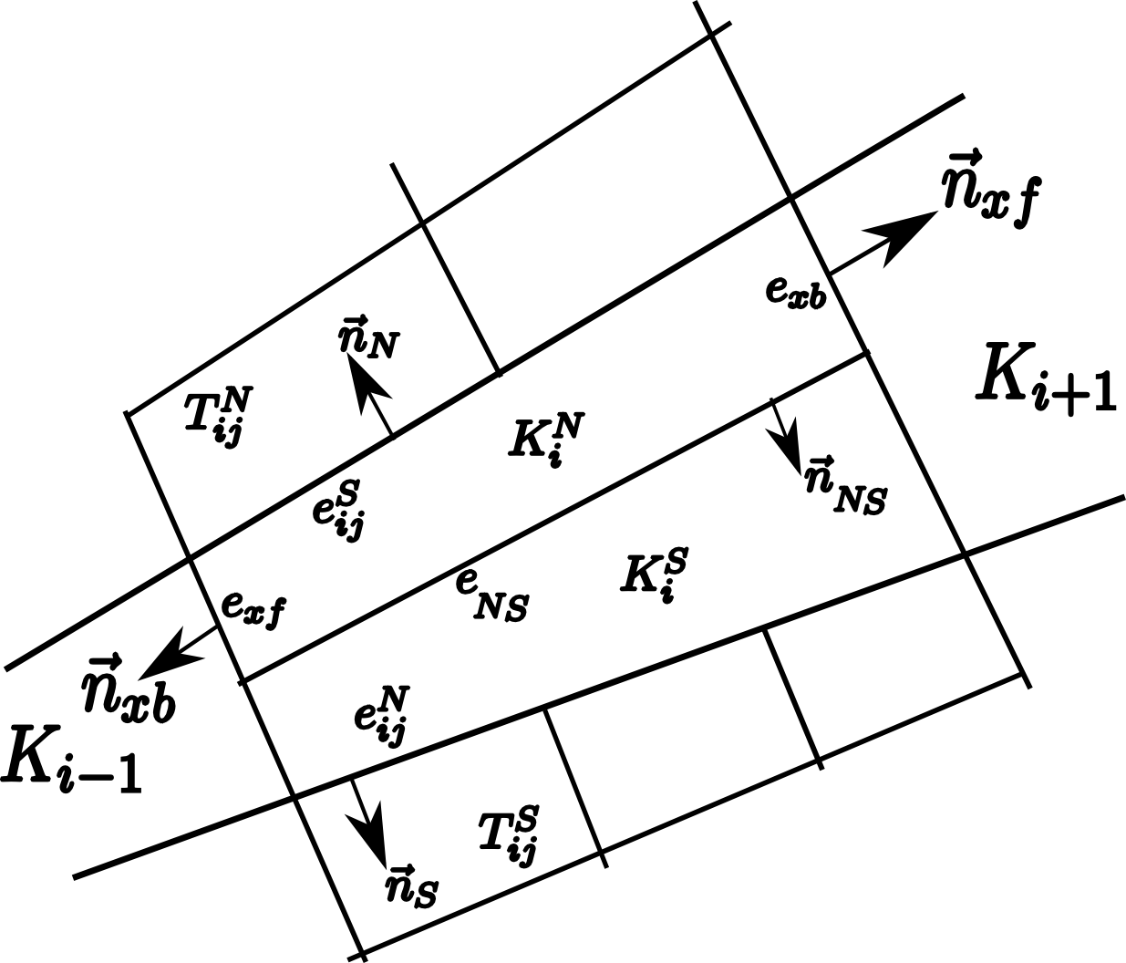
(b) The single 1D cell subdivided into two subcells KiNsubscriptsuperscript𝐾𝑁𝑖K^{N}_{i} and KiSsubscriptsuperscript𝐾𝑆𝑖K^{S}_{i} which are then viewed as 2D cells. exf,eNS,exbsubscript𝑒𝑥𝑓subscript𝑒𝑁𝑆subscript𝑒𝑥𝑏e_{xf},e_{NS},e_{xb} and eijN,j=1,2,Nnformulae-sequencesuperscriptsubscript𝑒𝑖𝑗𝑁𝑗12subscript𝑁𝑛e_{ij}^{N},j=1,2,...N_{n} are the edges of KiNsuperscriptsubscript𝐾𝑖𝑁K_{i}^{N} with their outward unit normal vectors as indicated. Similarly, the edges of KiSsuperscriptsubscript𝐾𝑖𝑆K_{i}^{S} and their normal vectors are indicated.
Figure 6: To the left is a 1D channel cell and its adjacent 2D floodplain cells while to the right is the 1D cell subdivided into two subcells viewed as 2D cells

Here, the goal to solve the lateral discharge model, (42) along the channel. Consider the 1D channel cell, KiΩh1Dsubscript𝐾𝑖superscriptsubscriptΩ1𝐷K_{i}\in\Omega_{h}^{1D}, with cell average vector 𝑾in=(Ain,Qin)Tsuperscriptsubscript𝑾𝑖𝑛superscriptsuperscriptsubscript𝐴𝑖𝑛superscriptsubscript𝑄𝑖𝑛𝑇\boldsymbol{W}_{i}^{n}=(A_{i}^{n},Q_{i}^{n})^{T} and denote by TijNΩh2D,j=1,2,,Nnformulae-sequencesuperscriptsubscript𝑇𝑖𝑗𝑁superscriptsubscriptΩ2𝐷𝑗12subscript𝑁𝑛T_{ij}^{N}\in\Omega_{h}^{2D},j=1,2,...,N_{n} and TijSΩh2D,j=1,2,,Nsformulae-sequencesuperscriptsubscript𝑇𝑖𝑗𝑆superscriptsubscriptΩ2𝐷𝑗12subscript𝑁𝑠T_{ij}^{S}\in\Omega_{h}^{2D},j=1,2,...,N_{s}, the j𝑗j-th 2D floodplain cells adjacent to Kisubscript𝐾𝑖K_{i} on its North edge eiNsuperscriptsubscript𝑒𝑖𝑁e_{i}^{N} and South edge eiSsuperscriptsubscript𝑒𝑖𝑆e_{i}^{S} respectively, see figure 6(a). Let the cell averages in the adjacent 2D cells TijNsuperscriptsubscript𝑇𝑖𝑗𝑁T_{ij}^{N} and TijSsuperscriptsubscript𝑇𝑖𝑗𝑆T_{ij}^{S} be

(ΠN)i,jn=((HN)i,jn,(qxN)i,jn,(qyN)i,jn)T and (ΠS)i,jn=((HS)i,jn,(qxS)i,jn,(qyS)i,jn)T,superscriptsubscriptsuperscriptΠ𝑁𝑖𝑗𝑛superscriptsuperscriptsubscriptsuperscript𝐻𝑁𝑖𝑗𝑛superscriptsubscriptsuperscriptsubscript𝑞𝑥𝑁𝑖𝑗𝑛superscriptsubscriptsuperscriptsubscript𝑞𝑦𝑁𝑖𝑗𝑛𝑇 and superscriptsubscriptsuperscriptΠ𝑆𝑖𝑗𝑛superscriptsuperscriptsubscriptsuperscript𝐻𝑆𝑖𝑗𝑛superscriptsubscriptsuperscriptsubscript𝑞𝑥𝑆𝑖𝑗𝑛superscriptsubscriptsuperscriptsubscript𝑞𝑦𝑆𝑖𝑗𝑛𝑇\begin{split}(\Pi^{N})_{i,j}^{n}=((H^{N})_{i,j}^{n},(q_{x}^{N})_{i,j}^{n},(q_{y}^{N})_{i,j}^{n})^{T}\mbox{ and }(\Pi^{S})_{i,j}^{n}=((H^{S})_{i,j}^{n},(q_{x}^{S})_{i,j}^{n},(q_{y}^{S})_{i,j}^{n})^{T},\end{split} (66)

respectively. Nnsubscript𝑁𝑛N_{n} and Nssubscript𝑁𝑠N_{s} are the number of the adjacent 2D cells on the North and South edges, respectively of Kisubscript𝐾𝑖K_{i}. (HN)ijn,(qxN)ijnsuperscriptsubscriptsuperscript𝐻𝑁𝑖𝑗𝑛superscriptsubscriptsuperscriptsubscript𝑞𝑥𝑁𝑖𝑗𝑛(H^{N})_{ij}^{n},(q_{x}^{N})_{ij}^{n} and (qyN)ijnsuperscriptsubscriptsuperscriptsubscript𝑞𝑦𝑁𝑖𝑗𝑛(q_{y}^{N})_{ij}^{n} are the average water depth, average discharge along x𝑥x-direction and average discharge along y𝑦y-direction respectively, in 2D cell TijNsuperscriptsubscript𝑇𝑖𝑗𝑁T_{ij}^{N} while (HS)ijn,(qxS)ijnsuperscriptsubscriptsuperscript𝐻𝑆𝑖𝑗𝑛superscriptsubscriptsuperscriptsubscript𝑞𝑥𝑆𝑖𝑗𝑛(H^{S})_{ij}^{n},(q_{x}^{S})_{ij}^{n} and (qyS)ijnsuperscriptsubscriptsuperscriptsubscript𝑞𝑦𝑆𝑖𝑗𝑛(q_{y}^{S})_{ij}^{n} are those of cell TijSsuperscriptsubscript𝑇𝑖𝑗𝑆T_{ij}^{S}.

To discretize the lateral discharge model (42) in Kisubscript𝐾𝑖K_{i}, we subdivide Kisubscript𝐾𝑖K_{i} into two subcells, KiNsuperscriptsubscript𝐾𝑖𝑁K_{i}^{N} and KiSsubscriptsuperscript𝐾𝑆𝑖K^{S}_{i} and view them as 2D cells within the channel, see figure 6(b). Let (𝑾N)insuperscriptsubscriptsuperscript𝑾𝑁𝑖𝑛(\boldsymbol{W}^{N})_{i}^{n} and (𝑾S)insuperscriptsubscriptsuperscript𝑾𝑆𝑖𝑛(\boldsymbol{W}^{S})_{i}^{n} be the 2D cell average vectors in the subcells, KiNsuperscriptsubscript𝐾𝑖𝑁K_{i}^{N} and KiSsuperscriptsubscript𝐾𝑖𝑆K_{i}^{S} respectively. Then, we define them as

(𝑾N)in=(H¯in,H¯inu¯in,(qyN)in)T and (𝑾S)in=(H¯in,H¯inu¯in,(qyS)in)T,superscriptsubscriptsuperscript𝑾𝑁𝑖𝑛superscriptsuperscriptsubscript¯𝐻𝑖𝑛superscriptsubscript¯𝐻𝑖𝑛superscriptsubscript¯𝑢𝑖𝑛superscriptsubscriptsuperscriptsubscript𝑞𝑦𝑁𝑖𝑛𝑇 and superscriptsubscriptsuperscript𝑾𝑆𝑖𝑛superscriptsuperscriptsubscript¯𝐻𝑖𝑛superscriptsubscript¯𝐻𝑖𝑛superscriptsubscript¯𝑢𝑖𝑛superscriptsubscriptsuperscriptsubscript𝑞𝑦𝑆𝑖𝑛𝑇(\boldsymbol{W}^{N})_{i}^{n}=(\underline{H}_{i}^{n},\underline{H}_{i}^{n}\underline{u}_{i}^{n},(q_{y}^{N})_{i}^{n})^{T}\mbox{ and }(\boldsymbol{W}^{S})_{i}^{n}=(\underline{H}_{i}^{n},\underline{H}_{i}^{n}\underline{u}_{i}^{n},(q_{y}^{S})_{i}^{n})^{T}, (67)

where H¯insuperscriptsubscript¯𝐻𝑖𝑛\underline{H}_{i}^{n} and u¯in=QinAinsuperscriptsubscript¯𝑢𝑖𝑛subscriptsuperscript𝑄𝑛𝑖superscriptsubscript𝐴𝑖𝑛\underline{u}_{i}^{n}=\frac{Q^{n}_{i}}{A_{i}^{n}} are the 1D cell average water depth and section-averaged velocity in the channel, and (qyS)in,(qyN)insuperscriptsubscriptsuperscriptsubscript𝑞𝑦𝑆𝑖𝑛superscriptsubscriptsuperscriptsubscript𝑞𝑦𝑁𝑖𝑛(q_{y}^{S})_{i}^{n},(q_{y}^{N})_{i}^{n} are computed at every time step using the scheme presented below.

The motivation to compute qyN/Ssuperscriptsubscript𝑞𝑦𝑁𝑆q_{y}^{N/S} is to apply a well-balanced scheme to the model,(42) in the subcells KiN/Ssuperscriptsubscript𝐾𝑖𝑁𝑆K_{i}^{N/S} by taking the bottom to be flat across all the edges within the channel, exb,eNS,exfsubscript𝑒𝑥𝑏subscript𝑒𝑁𝑆subscript𝑒𝑥𝑓e_{xb},e_{NS},e_{xf} (see figure 6(b)). To this end, we define the following:

h2ijNsuperscriptsubscript2𝑖𝑗𝑁\displaystyle h_{2ij}^{N} =max(0,η¯inzb,ijN),(𝑾~N)in=(h2ijN,h2ijNu¯in,h2ijN(vN)in)T,(vN)in=(qyN)in/H¯in,formulae-sequenceabsent𝑚𝑎𝑥0superscriptsubscript¯𝜂𝑖𝑛superscriptsubscript𝑧𝑏𝑖𝑗𝑁formulae-sequencesuperscriptsubscriptsuperscript~𝑾𝑁𝑖𝑛superscriptsuperscriptsubscript2𝑖𝑗𝑁superscriptsubscript2𝑖𝑗𝑁superscriptsubscript¯𝑢𝑖𝑛superscriptsubscript2𝑖𝑗𝑁superscriptsubscriptsuperscript𝑣𝑁𝑖𝑛𝑇superscriptsubscriptsuperscript𝑣𝑁𝑖𝑛superscriptsubscriptsuperscriptsubscript𝑞𝑦𝑁𝑖𝑛superscriptsubscript¯𝐻𝑖𝑛\displaystyle=max(0,\bar{\eta}_{i}^{n}-z_{b,ij}^{N}),\quad(\tilde{\boldsymbol{W}}^{N})_{i}^{n}=(h_{2ij}^{N},h_{2ij}^{N}\underline{u}_{i}^{n},h_{2ij}^{N}(v^{N})_{i}^{n})^{T},\quad(v^{N})_{i}^{n}=(q_{y}^{N})_{i}^{n}/\underline{H}_{i}^{n}, (68)

where η¯in=H¯in+Zb,isuperscriptsubscript¯𝜂𝑖𝑛superscriptsubscript¯𝐻𝑖𝑛subscript𝑍𝑏𝑖\bar{\eta}_{i}^{n}=\underline{H}_{i}^{n}+Z_{b,i} is the discrete flat free surface elevation in 1D cell, Kisubscript𝐾𝑖K_{i} and zb,ijNsuperscriptsubscript𝑧𝑏𝑖𝑗𝑁z_{b,ij}^{N} is the bed elevation of the adjacent 2D cell TijNsuperscriptsubscript𝑇𝑖𝑗𝑁T_{ij}^{N}, see figure 6(b). Therefore, we propose the following hydrostatic reconstruction scheme [1] for the lateral discharge in subcell KiNsuperscriptsubscript𝐾𝑖𝑁K_{i}^{N}:

(qyN)in+1=(qyN)inΔt|KiN|[|exb|ϕ32D((𝑾N)in,(𝑾N)i1n,nxb)+|exf|ϕ32D((𝑾N)in,(𝑾N)i+1n,nxf)+|eNS|ϕ32D((𝑾N)in,(𝑾S)in,nNS)]Δt|KiN|j=1Nn|eijN|[ϕ32D((𝑾~N)in,(ΠN)ijn,nN)+g2nN(0(H¯in)2(h2ijN)2)],superscriptsubscriptsuperscriptsubscript𝑞𝑦𝑁𝑖𝑛1superscriptsubscriptsuperscriptsubscript𝑞𝑦𝑁𝑖𝑛Δ𝑡superscriptsubscript𝐾𝑖𝑁delimited-[]subscript𝑒𝑥𝑏superscriptsubscriptitalic-ϕ32𝐷superscriptsubscriptsuperscript𝑾𝑁𝑖𝑛superscriptsubscriptsuperscript𝑾𝑁𝑖1𝑛subscript𝑛𝑥𝑏subscript𝑒𝑥𝑓superscriptsubscriptitalic-ϕ32𝐷superscriptsubscriptsuperscript𝑾𝑁𝑖𝑛superscriptsubscriptsuperscript𝑾𝑁𝑖1𝑛subscript𝑛𝑥𝑓subscript𝑒𝑁𝑆superscriptsubscriptitalic-ϕ32𝐷superscriptsubscriptsuperscript𝑾𝑁𝑖𝑛superscriptsubscriptsuperscript𝑾𝑆𝑖𝑛subscript𝑛𝑁𝑆Δ𝑡superscriptsubscript𝐾𝑖𝑁superscriptsubscript𝑗1𝑁𝑛superscriptsubscript𝑒𝑖𝑗𝑁delimited-[]superscriptsubscriptitalic-ϕ32𝐷superscriptsubscriptsuperscript~𝑾𝑁𝑖𝑛subscriptsuperscriptsuperscriptΠ𝑁𝑛𝑖𝑗subscript𝑛𝑁𝑔2subscript𝑛𝑁matrix0superscriptsuperscriptsubscript¯𝐻𝑖𝑛2superscriptsuperscriptsubscript2𝑖𝑗𝑁2\displaystyle\begin{split}(q_{y}^{N})_{i}^{n+1}=&(q_{y}^{N})_{i}^{n}-\frac{\Delta t}{|K_{i}^{N}|}\bigg{[}|e_{xb}|\phi_{3}^{2D}((\boldsymbol{W}^{N})_{i}^{n},(\boldsymbol{W}^{N})_{i-1}^{n},\vec{n}_{xb})+|e_{xf}|\phi_{3}^{2D}((\boldsymbol{W}^{N})_{i}^{n},(\boldsymbol{W}^{N})_{i+1}^{n},\vec{n}_{xf})\\ &+|e_{NS}|\phi_{3}^{2D}((\boldsymbol{W}^{N})_{i}^{n},(\boldsymbol{W}^{S})_{i}^{n},\vec{n}_{NS})\bigg{]}-\frac{\Delta t}{|K_{i}^{N}|}\sum_{j=1}^{Nn}|e_{ij}^{N}|\bigg{[}\phi_{3}^{2D}((\tilde{\boldsymbol{W}}^{N})_{i}^{n},(\Pi^{N})^{n}_{ij},\vec{n}_{N})\\ &+\frac{g}{2}\vec{n}_{N}\cdot\begin{pmatrix}0\\ (\underline{H}_{i}^{n})^{2}-(h_{2ij}^{N})^{2}\end{pmatrix}\bigg{]},\end{split} (69)

ϕ32D(wL,wR,n)superscriptsubscriptitalic-ϕ32𝐷subscript𝑤𝐿subscript𝑤𝑅𝑛\phi_{3}^{2D}(w_{L},w_{R},\vec{n}) denotes the 3rd component of numerical flux, ϕ2D(wL,wR,n):=Tn1ϕ(TnwL,TnwR)assignsuperscriptitalic-ϕ2𝐷subscript𝑤𝐿subscript𝑤𝑅𝑛superscriptsubscript𝑇𝑛1italic-ϕsubscript𝑇𝑛subscript𝑤𝐿subscript𝑇𝑛subscript𝑤𝑅\phi^{2D}(w_{L},w_{R},\vec{n}):=T_{\vec{n}}^{-1}\phi(T_{\vec{n}}w_{L},T_{\vec{n}}w_{R}). The quantities; |exb|,|exf|,|eNS|subscript𝑒𝑥𝑏subscript𝑒𝑥𝑓subscript𝑒𝑁𝑆|e_{xb}|,|e_{xf}|,|e_{NS}| and |eijN|superscriptsubscript𝑒𝑖𝑗𝑁|e_{ij}^{N}| are the lengths of the corresponding edges of KiNsuperscriptsubscript𝐾𝑖𝑁K_{i}^{N} and nNsubscript𝑛𝑁\vec{n}_{N} is the outward unit normal of KiNsuperscriptsubscript𝐾𝑖𝑁K_{i}^{N} towards TijNsuperscriptsubscript𝑇𝑖𝑗𝑁T_{ij}^{N} (see figure 6(b)).

Similarly, by defining

h2ijSsuperscriptsubscript2𝑖𝑗𝑆\displaystyle h_{2ij}^{S} =max(0,η¯inzb,ijS),(𝑾~S)in:=(h2ijS,h2ijSu¯in,h2ijS(vS)in)T,(vS)in:=(qyS)in/H¯in,formulae-sequenceabsent𝑚𝑎𝑥0superscriptsubscript¯𝜂𝑖𝑛superscriptsubscript𝑧𝑏𝑖𝑗𝑆formulae-sequenceassignsuperscriptsubscriptsuperscript~𝑾𝑆𝑖𝑛superscriptsuperscriptsubscript2𝑖𝑗𝑆superscriptsubscript2𝑖𝑗𝑆superscriptsubscript¯𝑢𝑖𝑛superscriptsubscript2𝑖𝑗𝑆superscriptsubscriptsuperscript𝑣𝑆𝑖𝑛𝑇assignsuperscriptsubscriptsuperscript𝑣𝑆𝑖𝑛superscriptsubscriptsuperscriptsubscript𝑞𝑦𝑆𝑖𝑛superscriptsubscript¯𝐻𝑖𝑛\displaystyle=max(0,\bar{\eta}_{i}^{n}-z_{b,ij}^{S}),\quad(\tilde{\boldsymbol{W}}^{S})_{i}^{n}:=(h_{2ij}^{S},h_{2ij}^{S}\underline{u}_{i}^{n},h_{2ij}^{S}(v^{S})_{i}^{n})^{T},\quad(v^{S})_{i}^{n}:=(q_{y}^{S})_{i}^{n}/\underline{H}_{i}^{n}, (70)

we propose the following scheme for the lateral discharge in KiSsuperscriptsubscript𝐾𝑖𝑆K_{i}^{S}:

(qyS)in+1=(qyS)inΔt|KiS|[|exb|ϕ32D((𝑾S)in,(𝑾S)i1n,nxb)+|exf|ϕ32D((𝑾S)in,(𝑾S)i+1n,nxf)+|eSN|ϕ32D((𝑾S)in,(𝑾N)in,nSN)]Δt|KiS|j=1Ns|eijS|[ϕ32D((𝑾~S)in,(ΠS)ijn,nS)+g2nN(0(H¯in)2(h2ijS)2)],superscriptsubscriptsuperscriptsubscript𝑞𝑦𝑆𝑖𝑛1superscriptsubscriptsuperscriptsubscript𝑞𝑦𝑆𝑖𝑛Δ𝑡superscriptsubscript𝐾𝑖𝑆delimited-[]subscript𝑒𝑥𝑏superscriptsubscriptitalic-ϕ32𝐷superscriptsubscriptsuperscript𝑾𝑆𝑖𝑛superscriptsubscriptsuperscript𝑾𝑆𝑖1𝑛subscript𝑛𝑥𝑏subscript𝑒𝑥𝑓superscriptsubscriptitalic-ϕ32𝐷superscriptsubscriptsuperscript𝑾𝑆𝑖𝑛superscriptsubscriptsuperscript𝑾𝑆𝑖1𝑛subscript𝑛𝑥𝑓subscript𝑒𝑆𝑁superscriptsubscriptitalic-ϕ32𝐷superscriptsubscriptsuperscript𝑾𝑆𝑖𝑛superscriptsubscriptsuperscript𝑾𝑁𝑖𝑛subscript𝑛𝑆𝑁Δ𝑡superscriptsubscript𝐾𝑖𝑆superscriptsubscript𝑗1𝑁𝑠superscriptsubscript𝑒𝑖𝑗𝑆delimited-[]superscriptsubscriptitalic-ϕ32𝐷superscriptsubscriptsuperscript~𝑾𝑆𝑖𝑛superscriptsubscriptsuperscriptΠ𝑆𝑖𝑗𝑛subscript𝑛𝑆𝑔2subscript𝑛𝑁matrix0superscriptsuperscriptsubscript¯𝐻𝑖𝑛2superscriptsuperscriptsubscript2𝑖𝑗𝑆2\displaystyle\begin{split}(q_{y}^{S})_{i}^{n+1}=&(q_{y}^{S})_{i}^{n}-\frac{\Delta t}{|K_{i}^{S}|}\bigg{[}|e_{xb}|\phi_{3}^{2D}((\boldsymbol{W}^{S})_{i}^{n},(\boldsymbol{W}^{S})_{i-1}^{n},\vec{n}_{xb})+|e_{xf}|\phi_{3}^{2D}((\boldsymbol{W}^{S})_{i}^{n},(\boldsymbol{W}^{S})_{i+1}^{n},\vec{n}_{xf})\\ &+|e_{SN}|\phi_{3}^{2D}((\boldsymbol{W}^{S})_{i}^{n},(\boldsymbol{W}^{N})_{i}^{n},\vec{n}_{SN})\bigg{]}-\frac{\Delta t}{|K_{i}^{S}|}\sum_{j=1}^{Ns}|e_{ij}^{S}|\bigg{[}\phi_{3}^{2D}((\tilde{\boldsymbol{W}}^{S})_{i}^{n},(\Pi^{S})_{ij}^{n},\vec{n}_{S})\\ &+\frac{g}{2}\vec{n}_{N}\cdot\begin{pmatrix}0\\ (\underline{H}_{i}^{n})^{2}-(h_{2ij}^{S})^{2}\end{pmatrix}\bigg{]},\end{split} (71)

where |eSN|subscript𝑒𝑆𝑁|e_{SN}| is length of edge, eSNsubscript𝑒𝑆𝑁e_{SN} between KiNsuperscriptsubscript𝐾𝑖𝑁K_{i}^{N} and KiSsuperscriptsubscript𝐾𝑖𝑆K_{i}^{S}, and zb,ijSsuperscriptsubscript𝑧𝑏𝑖𝑗𝑆z_{b,ij}^{S} is the bed elevation of 2D cell, TijSsuperscriptsubscript𝑇𝑖𝑗𝑆T_{ij}^{S}. The initial values of (qyS)in,(qyN)insuperscriptsubscriptsuperscriptsubscript𝑞𝑦𝑆𝑖𝑛superscriptsubscriptsuperscriptsubscript𝑞𝑦𝑁𝑖𝑛(q_{y}^{S})_{i}^{n},(q_{y}^{N})_{i}^{n} are obtained as explained in the following remark.

Remark 3.1

At initial time (n=0𝑛0n=0), only the lateral discharge, (qy)i0superscriptsubscriptsubscript𝑞𝑦𝑖0(q_{y})_{i}^{0} for the full cell, Kisubscript𝐾𝑖K_{i} is given. Then we initialize (qyN)i0superscriptsubscriptsuperscriptsubscript𝑞𝑦𝑁𝑖0(q_{y}^{N})_{i}^{0} and (qyS)i0superscriptsubscriptsuperscriptsubscript𝑞𝑦𝑆𝑖0(q_{y}^{S})_{i}^{0} to be equal to it, namely

(qyN)i0=(qyS)i0=(qy)i0.superscriptsubscriptsuperscriptsubscript𝑞𝑦𝑁𝑖0superscriptsubscriptsuperscriptsubscript𝑞𝑦𝑆𝑖0superscriptsubscriptsubscript𝑞𝑦𝑖0(q_{y}^{N})_{i}^{0}=(q_{y}^{S})_{i}^{0}=(q_{y})_{i}^{0}. (72)

For other times, (n>0𝑛0n>0), we compute (qyS/N)insuperscriptsubscriptsuperscriptsubscript𝑞𝑦𝑆𝑁𝑖𝑛(q_{y}^{S/N})_{i}^{n} using the scheme described above.

3.2.3 Discrete Coupling Terms

To discretize the coupling term, let us denote by fi,jSsuperscriptsubscript𝑓𝑖𝑗𝑆f_{i,j}^{S} the approximation of a function, f𝑓f at the edge, eijSsubscriptsuperscript𝑒𝑆𝑖𝑗e^{S}_{ij} between 1D cell Kisubscript𝐾𝑖K_{i} and 2D cell TijSsuperscriptsubscript𝑇𝑖𝑗𝑆T_{ij}^{S} (see figure 6(b)). Then the approximation, f|Levaluated-at𝑓𝐿f|_{L} of f𝑓f over the entire South edge, eiSsuperscriptsubscript𝑒𝑖𝑆e_{i}^{S} of Kisubscript𝐾𝑖K_{i}, is given by averaging over all edges on the South edge, namely

(f|L)i=j=1Ns(fi,jS|eijS||eiS|),subscriptevaluated-at𝑓𝐿𝑖superscriptsubscript𝑗1𝑁𝑠superscriptsubscript𝑓𝑖𝑗𝑆superscriptsubscript𝑒𝑖𝑗𝑆superscriptsubscript𝑒𝑖𝑆(f|_{L})_{i}=\sum_{j=1}^{Ns}\bigg{(}f_{i,j}^{S}\frac{|e_{ij}^{S}|}{|e_{i}^{S}|}\bigg{)}, (73)

where |eijS|subscriptsuperscript𝑒𝑆𝑖𝑗|e^{S}_{ij}| is the length of edge, eijSsuperscriptsubscript𝑒𝑖𝑗𝑆e_{ij}^{S}; |eiS|subscriptsuperscript𝑒𝑆𝑖|e^{S}_{i}| is sum of all edges of Kisubscript𝐾𝑖K_{i} on the South side. Similarly (f|R)i=j=1Nn(fi,jN|eijN||eiN|)subscriptevaluated-at𝑓𝑅𝑖superscriptsubscript𝑗1𝑁𝑛superscriptsubscript𝑓𝑖𝑗𝑁superscriptsubscript𝑒𝑖𝑗𝑁superscriptsubscript𝑒𝑖𝑁(f|_{R})_{i}=\sum_{j=1}^{Nn}\bigg{(}f_{i,j}^{N}\frac{|e_{ij}^{N}|}{|e_{i}^{N}|}\bigg{)} for North edge, where |eijN|subscriptsuperscript𝑒𝑁𝑖𝑗|e^{N}_{ij}| is the length of edge between Kisubscript𝐾𝑖K_{i} and TijNsuperscriptsubscript𝑇𝑖𝑗𝑁T_{ij}^{N}, and |eiN|superscriptsubscript𝑒𝑖𝑁|e_{i}^{N}| is the sum of all edges on North side of Kisubscript𝐾𝑖K_{i}. Hence we can approximate the coupling term as

Φin=j=1NsΨi,jS+j=1NnΨi,jN,superscriptsubscriptΦ𝑖𝑛superscriptsubscript𝑗1𝑁𝑠superscriptsubscriptΨ𝑖𝑗𝑆superscriptsubscript𝑗1𝑁𝑛superscriptsubscriptΨ𝑖𝑗𝑁\displaystyle\Phi_{i}^{n}=\sum_{j=1}^{Ns}\Psi_{i,j}^{S}+\sum_{j=1}^{Nn}\Psi_{i,j}^{N}, (74)

where

Ψi,jS=(1nSyfi,j1,S1nSyfi,j2,SnSxnSyg2(Hi,jS)2)|eijS||eiS|,Ψi,jN=(1nNyfi,j1,N1nNyfi,j2,N+nNxnNyg2(Hi,jN)2)|eijN||eiN|,formulae-sequencesubscriptsuperscriptΨ𝑆𝑖𝑗matrix1subscriptsuperscript𝑛𝑦𝑆subscriptsuperscript𝑓1𝑆𝑖𝑗1subscriptsuperscript𝑛𝑦𝑆subscriptsuperscript𝑓2𝑆𝑖𝑗subscriptsuperscript𝑛𝑥𝑆subscriptsuperscript𝑛𝑦𝑆𝑔2superscriptsubscriptsuperscript𝐻𝑆𝑖𝑗2superscriptsubscript𝑒𝑖𝑗𝑆superscriptsubscript𝑒𝑖𝑆subscriptsuperscriptΨ𝑁𝑖𝑗matrix1subscriptsuperscript𝑛𝑦𝑁subscriptsuperscript𝑓1𝑁𝑖𝑗1subscriptsuperscript𝑛𝑦𝑁subscriptsuperscript𝑓2𝑁𝑖𝑗subscriptsuperscript𝑛𝑥𝑁subscriptsuperscript𝑛𝑦𝑁𝑔2superscriptsubscriptsuperscript𝐻𝑁𝑖𝑗2superscriptsubscript𝑒𝑖𝑗𝑁superscriptsubscript𝑒𝑖𝑁\displaystyle\Psi^{S}_{i,j}=\begin{pmatrix}\frac{1}{n^{y}_{S}}f^{1,S}_{i,j}\\ \frac{1}{n^{y}_{S}}f^{2,S}_{i,j}-\frac{n^{x}_{S}}{n^{y}_{S}}\frac{g}{2}(H^{S*}_{i,j})^{2}\end{pmatrix}\frac{|e_{ij}^{S}|}{|e_{i}^{S}|},\quad\Psi^{N}_{i,j}=\begin{pmatrix}-\frac{1}{n^{y}_{N}}f^{1,N}_{i,j}\\ -\frac{1}{n^{y}_{N}}f^{2,N}_{i,j}+\frac{n^{x}_{N}}{n^{y}_{N}}\frac{g}{2}(H^{N*}_{i,j})^{2}\end{pmatrix}\frac{|e_{ij}^{N}|}{|e_{i}^{N}|}, (75)

are the discrete coupling terms at the edges eijSsuperscriptsubscript𝑒𝑖𝑗𝑆e_{ij}^{S} and eijNsuperscriptsubscript𝑒𝑖𝑗𝑁e_{ij}^{N} respectively (see figure 6(b)). Hi,jS,fi,j1,Ssubscriptsuperscript𝐻𝑆𝑖𝑗subscriptsuperscript𝑓1𝑆𝑖𝑗H^{S*}_{i,j},f^{1,S}_{i,j} and fi,j2,Ssubscriptsuperscript𝑓2𝑆𝑖𝑗f^{2,S}_{i,j} are respectively, the discrete water depth, first and second components of 2D numerical flux at edge eijSsuperscriptsubscript𝑒𝑖𝑗𝑆e_{ij}^{S}. While Hi,jN,fi,j1,Nsubscriptsuperscript𝐻𝑁𝑖𝑗subscriptsuperscript𝑓1𝑁𝑖𝑗H^{N*}_{i,j},f^{1,N}_{i,j} and fi,j2,Nsubscriptsuperscript𝑓2𝑁𝑖𝑗f^{2,N}_{i,j} are respectively, the water depth, first and second components of 2D numerical flux at edge, eijNsuperscriptsubscript𝑒𝑖𝑗𝑁e_{ij}^{N}. We now focus on how to compute them.

Given the 1D cell average, 𝑾insuperscriptsubscript𝑾𝑖𝑛\boldsymbol{W}_{i}^{n} in Kisubscript𝐾𝑖K_{i} from which we obtain the cell average (𝑾S)insuperscriptsubscriptsuperscript𝑾𝑆𝑖𝑛(\boldsymbol{W}^{S})_{i}^{n} in the subcell, KiSsuperscriptsubscript𝐾𝑖𝑆K_{i}^{S} (using equation (67)). Then we directly approximate fi,j1,Ssubscriptsuperscript𝑓1𝑆𝑖𝑗f^{1,S}_{i,j} and fi,j2,Ssubscriptsuperscript𝑓2𝑆𝑖𝑗f^{2,S}_{i,j} by computing the 2D numerical flux, ϕ2D((𝑾~S)in,(ΠS)ijn,nS)superscriptitalic-ϕ2𝐷subscriptsuperscriptsuperscript~𝑾𝑆𝑛𝑖superscriptsubscriptsuperscriptΠ𝑆𝑖𝑗𝑛subscript𝑛𝑆\phi^{2D}((\tilde{\boldsymbol{W}}^{S})^{n}_{i},(\Pi^{S})_{ij}^{n},\vec{n}_{S}), at edge, eijSsuperscriptsubscript𝑒𝑖𝑗𝑆e_{ij}^{S} (see figure 6(b)), namely

fi,j1,S=ϕ12D((𝑾~S)in,(ΠS)ijn,nS),fi,j2,S=ϕ22D((𝑾~S)in,(ΠS)ijn,nS).\begin{split}f^{1,S}_{i,j}=\phi_{1}^{2D}((\tilde{\boldsymbol{W}}^{S})^{n}_{i},(\Pi^{S})_{ij}^{n},\vec{n}_{S}),\quad f^{2,S}_{i,j}=\phi_{2}^{2D}((\tilde{\boldsymbol{W}}^{S})^{n}_{i},(\Pi^{S})_{ij}^{n},\vec{n}_{S}).\end{split} (76)

Similarly, by using (𝑾~N)insubscriptsuperscriptsuperscript~𝑾𝑁𝑛𝑖(\tilde{\boldsymbol{W}}^{N})^{n}_{i} and (ΠN)ijnsuperscriptsubscriptsuperscriptΠ𝑁𝑖𝑗𝑛(\Pi^{N})_{ij}^{n} we approximate fi,j1,Nsubscriptsuperscript𝑓1𝑁𝑖𝑗f^{1,N}_{i,j} and fi,j2,Nsubscriptsuperscript𝑓2𝑁𝑖𝑗f^{2,N}_{i,j} using

fi,j1,N=ϕ12D((𝑾~N)in,(ΠN)ijn,nN),fi,j2,N=ϕ22D((𝑾~N)in,(ΠN)ijn,nN),\begin{split}f^{1,N}_{i,j}=\phi_{1}^{2D}((\tilde{\boldsymbol{W}}^{N})^{n}_{i},(\Pi^{N})_{ij}^{n},\vec{n}_{N}),\quad f^{2,N}_{i,j}=\phi_{2}^{2D}((\tilde{\boldsymbol{W}}^{N})^{n}_{i},(\Pi^{N})_{ij}^{n},\vec{n}_{N}),\end{split} (77)

The hydrostatically reconstructed quantities, (𝑾~N)insubscriptsuperscriptsuperscript~𝑾𝑁𝑛𝑖(\tilde{\boldsymbol{W}}^{N})^{n}_{i} and (𝑾~S)insubscriptsuperscriptsuperscript~𝑾𝑆𝑛𝑖(\tilde{\boldsymbol{W}}^{S})^{n}_{i} are defined in equations (68) and (70) respectively.

To approximate Hi,jSsuperscriptsubscript𝐻𝑖𝑗𝑆H_{i,j}^{S*} and Hi,jNsuperscriptsubscript𝐻𝑖𝑗𝑁H_{i,j}^{N*}, we propose to adapt the hydrostatic reconstruction approach [1], namely

Hi,jS=max(h2ijS,(HS)i,jn),Hi,jN=max(h2ijN,(HN)i,jn),formulae-sequencesuperscriptsubscript𝐻𝑖𝑗𝑆superscriptsubscript2𝑖𝑗𝑆superscriptsubscriptsuperscript𝐻𝑆𝑖𝑗𝑛superscriptsubscript𝐻𝑖𝑗𝑁superscriptsubscript2𝑖𝑗𝑁superscriptsubscriptsuperscript𝐻𝑁𝑖𝑗𝑛\displaystyle H_{i,j}^{S*}=\max(h_{2ij}^{S},(H^{S})_{i,j}^{n}),\quad H_{i,j}^{N*}=\max(h_{2ij}^{N},(H^{N})_{i,j}^{n}), (78)

We therefore summarise the discrete coupling term as

Φin=1|eiS|j=1Ns|eijS|(1nSyϕ12D((𝑾~S)in,(ΠS)ijn,nS)1nSyϕ22D((𝑾~S)in,(ΠS)ijn,nS)g2nSxnSy[max(h2ijS,(HS)ijn)]2)1|eiN|j=1Nn|eijN|(1nNyϕ12D((𝑾~N)in,(ΠN)ijn,nN)1nNyϕ22D((𝑾~N)in,(ΠN)ijn,nN)g2nNxnNy[max(h2ijN,(HN)ijn)]2),superscriptsubscriptΦ𝑖𝑛1superscriptsubscript𝑒𝑖𝑆superscriptsubscript𝑗1𝑁𝑠superscriptsubscript𝑒𝑖𝑗𝑆matrix1subscriptsuperscript𝑛𝑦𝑆superscriptsubscriptitalic-ϕ12𝐷superscriptsubscriptsuperscript~𝑾𝑆𝑖𝑛superscriptsubscriptsuperscriptΠ𝑆𝑖𝑗𝑛subscript𝑛𝑆1subscriptsuperscript𝑛𝑦𝑆superscriptsubscriptitalic-ϕ22𝐷superscriptsubscriptsuperscript~𝑾𝑆𝑖𝑛superscriptsubscriptsuperscriptΠ𝑆𝑖𝑗𝑛subscript𝑛𝑆𝑔2superscriptsubscript𝑛𝑆𝑥superscriptsubscript𝑛𝑆𝑦superscriptdelimited-[]superscriptsubscript2𝑖𝑗𝑆superscriptsubscriptsuperscript𝐻𝑆𝑖𝑗𝑛21superscriptsubscript𝑒𝑖𝑁superscriptsubscript𝑗1subscript𝑁𝑛superscriptsubscript𝑒𝑖𝑗𝑁matrix1subscriptsuperscript𝑛𝑦𝑁superscriptsubscriptitalic-ϕ12𝐷superscriptsubscriptsuperscript~𝑾𝑁𝑖𝑛superscriptsubscriptsuperscriptΠ𝑁𝑖𝑗𝑛subscript𝑛𝑁1subscriptsuperscript𝑛𝑦𝑁superscriptsubscriptitalic-ϕ22𝐷superscriptsubscriptsuperscript~𝑾𝑁𝑖𝑛superscriptsubscriptsuperscriptΠ𝑁𝑖𝑗𝑛subscript𝑛𝑁𝑔2superscriptsubscript𝑛𝑁𝑥superscriptsubscript𝑛𝑁𝑦superscriptdelimited-[]superscriptsubscript2𝑖𝑗𝑁superscriptsubscriptsuperscript𝐻𝑁𝑖𝑗𝑛2\displaystyle\begin{split}\Phi_{i}^{n}&=\frac{1}{|e_{i}^{S}|}\sum_{j=1}^{Ns}|e_{ij}^{S}|\begin{pmatrix}\frac{1}{n^{y}_{S}}\phi_{1}^{2D}((\tilde{\boldsymbol{W}}^{S})_{i}^{n},(\Pi^{S})_{ij}^{n},\vec{n}_{S})\\ \frac{1}{n^{y}_{S}}\phi_{2}^{2D}((\tilde{\boldsymbol{W}}^{S})_{i}^{n},(\Pi^{S})_{ij}^{n},\vec{n}_{S})-\frac{g}{2}\frac{n_{S}^{x}}{n_{S}^{y}}\bigg{[}\max(h_{2ij}^{S},(H^{S})_{ij}^{n})\bigg{]}^{2}\end{pmatrix}\\ &-\frac{1}{|e_{i}^{N}|}\sum_{j=1}^{N_{n}}|e_{ij}^{N}|\begin{pmatrix}\frac{1}{n^{y}_{N}}\phi_{1}^{2D}((\tilde{\boldsymbol{W}}^{N})_{i}^{n},(\Pi^{N})_{ij}^{n},\vec{n}_{N})\\ \frac{1}{n^{y}_{N}}\phi_{2}^{2D}((\tilde{\boldsymbol{W}}^{N})_{i}^{n},(\Pi^{N})_{ij}^{n},\vec{n}_{N})-\frac{g}{2}\frac{n_{N}^{x}}{n_{N}^{y}}\bigg{[}\max(h_{2ij}^{N},(H^{N})_{ij}^{n})\bigg{]}^{2}\end{pmatrix},\end{split} (79)
nNy,nSy0.superscriptsubscript𝑛𝑁𝑦superscriptsubscript𝑛𝑆𝑦0\displaystyle n_{N}^{y},n_{S}^{y}\neq 0.

3.3 Summary of the Channel Flow Solver

The complete scheme for the channel flow model with coupling term, (40)-(41) is

𝑾in+1=𝑾in+1+ΔtΦin,superscriptsubscript𝑾𝑖𝑛1superscriptsubscript𝑾𝑖𝑛1Δ𝑡superscriptsubscriptΦ𝑖𝑛\boldsymbol{W}_{i}^{n+1}=\boldsymbol{W}_{i}^{n+1*}+\Delta t\Phi_{i}^{n}, (80)

where 𝑾in+1superscriptsubscript𝑾𝑖𝑛1\boldsymbol{W}_{i}^{n+1*} is the solution of the purely channel model without the coupling terms,(54) which is given in (64). ΦinsuperscriptsubscriptΦ𝑖𝑛\Phi_{i}^{n} is the discrete coupling term summarised in (79). The channel lateral discharges are computed using the schemes in (69) and (71).

3.4 Summary of the Horizontal Coupling Method

The channel flow model, (40), (41) and (42) is simulated as summarised in section 3.3 while the flood flow model, (43) is solved with the 2D solver, (46). At 2D/1D edge, the 2D numerical flux is computed by using the 2D cell, TjΩh2Dsubscript𝑇𝑗superscriptsubscriptΩ2𝐷T_{j}\in\Omega_{h}^{2D} averages and the averages obtained from the adjacent channel subcell, (KiNsuperscriptsubscript𝐾𝑖𝑁K_{i}^{N} or KiSsuperscriptsubscript𝐾𝑖𝑆K_{i}^{S}) as described in (67). A flow chart for the implementation of the HCM is given in figure 7.
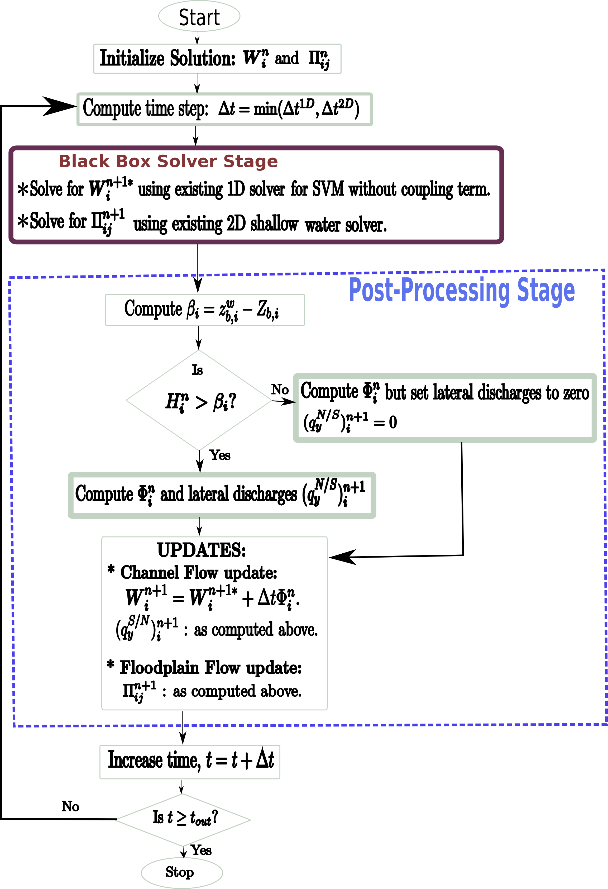
Refer to caption
Figure 7: Flow Chart for implementation of the Horizontal Coupling Method (HCM)

4 Properties of the HCM

We discuss a few properties of the method in this section.

Definition 4.1 (Well Balance of Lake at rest)

Assuming that the existing numerical schemes for the uncoupled 1D and 2D models are well balanced with respect to lake at rest, then the coupled scheme is said to be well balanced with respect to lake at rest if the coupling term vanishes whenever the lake at rest condition holds.

Theorem 4.1

The coupling term derived in equation (79) leads to a fully well-balanced scheme with respect to lake at rest.

proof 4.1

Assuming that the condition of water at rest holds, then

η¯in=(ηN)ijn=(ηS)ijnjformulae-sequencesuperscriptsubscript¯𝜂𝑖𝑛superscriptsubscriptsuperscript𝜂𝑁𝑖𝑗𝑛superscriptsubscriptsuperscript𝜂𝑆𝑖𝑗𝑛for-all𝑗\bar{\eta}_{i}^{n}=(\eta^{N})_{ij}^{n}=(\eta^{S})_{ij}^{n}\quad\forall j

where (ηS)ijnsuperscriptsubscriptsuperscript𝜂𝑆𝑖𝑗𝑛(\eta^{S})_{ij}^{n} and (ηN)ijnsuperscriptsubscriptsuperscript𝜂𝑁𝑖𝑗𝑛(\eta^{N})_{ij}^{n} are the free surface elevation in the adjacent 2D cells, TijSsuperscriptsubscript𝑇𝑖𝑗𝑆T_{ij}^{S} and TijNsuperscriptsubscript𝑇𝑖𝑗𝑁T_{ij}^{N} respectively. Hence,

h2,ijS:=max(0,η¯inzb,ijS)=max(0,(ηS)ijnzb,ijS)=max(0,(HS)ijn)=(HS)ijn,h2,ijN:=max(0,η¯inzb,ijN)=max(0,(ηN)ijnzb,ijN)=(HN)ijn.formulae-sequenceassignsuperscriptsubscript2𝑖𝑗𝑆0superscriptsubscript¯𝜂𝑖𝑛superscriptsubscript𝑧𝑏𝑖𝑗𝑆0superscriptsubscriptsuperscript𝜂𝑆𝑖𝑗𝑛superscriptsubscript𝑧𝑏𝑖𝑗𝑆0superscriptsubscriptsuperscript𝐻𝑆𝑖𝑗𝑛superscriptsubscriptsuperscript𝐻𝑆𝑖𝑗𝑛assignsuperscriptsubscript2𝑖𝑗𝑁0superscriptsubscript¯𝜂𝑖𝑛superscriptsubscript𝑧𝑏𝑖𝑗𝑁0superscriptsubscriptsuperscript𝜂𝑁𝑖𝑗𝑛superscriptsubscript𝑧𝑏𝑖𝑗𝑁superscriptsubscriptsuperscript𝐻𝑁𝑖𝑗𝑛\displaystyle\begin{split}&h_{2,ij}^{S}:=\max(0,\bar{\eta}_{i}^{n}-z_{b,ij}^{S})=\max(0,(\eta^{S})_{ij}^{n}-z_{b,ij}^{S})=\max(0,(H^{S})_{ij}^{n})=(H^{S})_{ij}^{n},\\ &h_{2,ij}^{N}:=\max(0,\bar{\eta}_{i}^{n}-z_{b,ij}^{N})=\max(0,(\eta^{N})_{ij}^{n}-z_{b,ij}^{N})=(H^{N})_{ij}^{n}.\end{split}

Therefore,

max(h2ijS,(HS)ijn)=h2ijS and max(h2ijN,(HN)ijn)=h2ijN.superscriptsubscript2𝑖𝑗𝑆superscriptsubscriptsuperscript𝐻𝑆𝑖𝑗𝑛superscriptsubscript2𝑖𝑗𝑆 and superscriptsubscript2𝑖𝑗𝑁superscriptsubscriptsuperscript𝐻𝑁𝑖𝑗𝑛superscriptsubscript2𝑖𝑗𝑁\displaystyle\max(h_{2ij}^{S},(H^{S})_{ij}^{n})=h_{2ij}^{S}\mbox{ and }\max(h_{2ij}^{N},(H^{N})_{ij}^{n})=h_{2ij}^{N}. (81)

Since all velocities (and discharges) are zero, then

(ΠS)ijn=((HS)ijn,0,0)T=(h2ijS,0,0)T=(𝑾~S)in.superscriptsubscriptsuperscriptΠ𝑆𝑖𝑗𝑛superscriptsuperscriptsubscriptsuperscript𝐻𝑆𝑖𝑗𝑛00𝑇superscriptsuperscriptsubscript2𝑖𝑗𝑆00𝑇superscriptsubscriptsuperscript~𝑾𝑆𝑖𝑛(\Pi^{S})_{ij}^{n}=((H^{S})_{ij}^{n},0,0)^{T}=(h_{2ij}^{S},0,0)^{T}=(\tilde{\boldsymbol{W}}^{S})_{i}^{n}.

Hence, by the consistency of the numerical flux, ϕ2Dsuperscriptitalic-ϕ2𝐷\phi^{2D} with the physical flux, F()𝐹F(\cdot), we have

ϕ2D((𝑾~S)in,(ΠS)ijn,𝒏S)=F((𝑾~S)in)𝒏S=(0,nSxg2[h2ijS]2,nSyg2[h2ijS]2)T.superscriptitalic-ϕ2𝐷superscriptsubscriptsuperscript~𝑾𝑆𝑖𝑛superscriptsubscriptsuperscriptΠ𝑆𝑖𝑗𝑛subscript𝒏𝑆𝐹superscriptsubscriptsuperscript~𝑾𝑆𝑖𝑛subscript𝒏𝑆superscript0superscriptsubscript𝑛𝑆𝑥𝑔2superscriptdelimited-[]superscriptsubscript2𝑖𝑗𝑆2superscriptsubscript𝑛𝑆𝑦𝑔2superscriptdelimited-[]superscriptsubscript2𝑖𝑗𝑆2𝑇\phi^{2D}((\tilde{\boldsymbol{W}}^{S})_{i}^{n},(\Pi^{S})_{ij}^{n},\vec{\boldsymbol{n}}_{S})=F((\tilde{\boldsymbol{W}}^{S})_{i}^{n})\cdot\vec{\boldsymbol{n}}_{S}=(0,n_{S}^{x}\frac{g}{2}\bigg{[}h_{2ij}^{S}\bigg{]}^{2},n_{S}^{y}\frac{g}{2}\bigg{[}h_{2ij}^{S}\bigg{]}^{2})^{T}.

That is

ϕ12D((𝑾~S)in,(ΠS)ijn,𝒏S)=0,ϕ22D((𝑾~S)in,(ΠS)ijn,𝒏S)=nSxg2[h2ijS]2.formulae-sequencesuperscriptsubscriptitalic-ϕ12𝐷superscriptsubscriptsuperscript~𝑾𝑆𝑖𝑛superscriptsubscriptsuperscriptΠ𝑆𝑖𝑗𝑛subscript𝒏𝑆0superscriptsubscriptitalic-ϕ22𝐷superscriptsubscriptsuperscript~𝑾𝑆𝑖𝑛superscriptsubscriptsuperscriptΠ𝑆𝑖𝑗𝑛subscript𝒏𝑆superscriptsubscript𝑛𝑆𝑥𝑔2superscriptdelimited-[]superscriptsubscript2𝑖𝑗𝑆2\displaystyle\phi_{1}^{2D}((\tilde{\boldsymbol{W}}^{S})_{i}^{n},(\Pi^{S})_{ij}^{n},\vec{\boldsymbol{n}}_{S})=0,\quad\phi_{2}^{2D}((\tilde{\boldsymbol{W}}^{S})_{i}^{n},(\Pi^{S})_{ij}^{n},\vec{\boldsymbol{n}}_{S})=n_{S}^{x}\frac{g}{2}\bigg{[}h_{2ij}^{S}\bigg{]}^{2}. (82)

Similarly,

(ΠN)jn=((HN)ijn,0,0)T=(𝑾~N)in and ϕ2D((𝑾~N)in,(ΠN)ijn,𝒏N)=(0,nNxg2[h2ijN]2,nNyg2[h2ijN]2)T.superscriptsubscriptsuperscriptΠ𝑁𝑗𝑛superscriptsuperscriptsubscriptsuperscript𝐻𝑁𝑖𝑗𝑛00𝑇superscriptsubscriptsuperscript~𝑾𝑁𝑖𝑛 and superscriptitalic-ϕ2𝐷superscriptsubscriptsuperscript~𝑾𝑁𝑖𝑛superscriptsubscriptsuperscriptΠ𝑁𝑖𝑗𝑛subscript𝒏𝑁superscript0superscriptsubscript𝑛𝑁𝑥𝑔2superscriptdelimited-[]superscriptsubscript2𝑖𝑗𝑁2superscriptsubscript𝑛𝑁𝑦𝑔2superscriptdelimited-[]superscriptsubscript2𝑖𝑗𝑁2𝑇\displaystyle\begin{split}(\Pi^{N})_{j}^{n}=((H^{N})_{ij}^{n},0,0)^{T}=(\tilde{\boldsymbol{W}}^{N})_{i}^{n}\mbox{ and }\phi^{2D}((\tilde{\boldsymbol{W}}^{N})_{i}^{n},(\Pi^{N})_{ij}^{n},\vec{\boldsymbol{n}}_{N})=(0,n_{N}^{x}\frac{g}{2}\bigg{[}h_{2ij}^{N}\bigg{]}^{2},n_{N}^{y}\frac{g}{2}\bigg{[}h_{2ij}^{N}\bigg{]}^{2})^{T}.\end{split}

So that

ϕ12D((𝑾~N)in,(ΠN)ijn,𝒏N)=0,ϕ22D((𝑾~N)in,(ΠN)ijn,𝒏N)=nNxg2[h2ijN]2.formulae-sequencesuperscriptsubscriptitalic-ϕ12𝐷superscriptsubscriptsuperscript~𝑾𝑁𝑖𝑛superscriptsubscriptsuperscriptΠ𝑁𝑖𝑗𝑛subscript𝒏𝑁0superscriptsubscriptitalic-ϕ22𝐷superscriptsubscriptsuperscript~𝑾𝑁𝑖𝑛superscriptsubscriptsuperscriptΠ𝑁𝑖𝑗𝑛subscript𝒏𝑁superscriptsubscript𝑛𝑁𝑥𝑔2superscriptdelimited-[]superscriptsubscript2𝑖𝑗𝑁2\displaystyle\phi_{1}^{2D}((\tilde{\boldsymbol{W}}^{N})_{i}^{n},(\Pi^{N})_{ij}^{n},\vec{\boldsymbol{n}}_{N})=0,\quad\phi_{2}^{2D}((\tilde{\boldsymbol{W}}^{N})_{i}^{n},(\Pi^{N})_{ij}^{n},\vec{\boldsymbol{n}}_{N})=n_{N}^{x}\frac{g}{2}\bigg{[}h_{2ij}^{N}\bigg{]}^{2}. (83)

Therefore, using equations (81)-(83), then the discrete coupling term in (79) becomes

Φin=1|eiS|j=1Ns|eijS|(01nSynSxg2[h2ijS]2g2nSxnSy[h2ijS]2)1|eiN|j=1Nn|eijN|(01nNynNxg2[h2ijN]2g2nNxnNy[h2ijN]2)=(00).superscriptsubscriptΦ𝑖𝑛1superscriptsubscript𝑒𝑖𝑆superscriptsubscript𝑗1𝑁𝑠superscriptsubscript𝑒𝑖𝑗𝑆matrix01subscriptsuperscript𝑛𝑦𝑆superscriptsubscript𝑛𝑆𝑥𝑔2superscriptdelimited-[]superscriptsubscript2𝑖𝑗𝑆2𝑔2superscriptsubscript𝑛𝑆𝑥superscriptsubscript𝑛𝑆𝑦superscriptdelimited-[]superscriptsubscript2𝑖𝑗𝑆21superscriptsubscript𝑒𝑖𝑁superscriptsubscript𝑗1𝑁𝑛superscriptsubscript𝑒𝑖𝑗𝑁matrix01subscriptsuperscript𝑛𝑦𝑁superscriptsubscript𝑛𝑁𝑥𝑔2superscriptdelimited-[]superscriptsubscript2𝑖𝑗𝑁2𝑔2superscriptsubscript𝑛𝑁𝑥superscriptsubscript𝑛𝑁𝑦superscriptdelimited-[]superscriptsubscript2𝑖𝑗𝑁2matrix00\displaystyle\begin{split}\Phi_{i}^{n}&=\frac{1}{|e_{i}^{S}|}\sum_{j=1}^{Ns}|e_{ij}^{S}|\begin{pmatrix}0\\ \frac{1}{n^{y}_{S}}n_{S}^{x}\frac{g}{2}\bigg{[}h_{2ij}^{S}\bigg{]}^{2}-\frac{g}{2}\frac{n_{S}^{x}}{n_{S}^{y}}\bigg{[}h_{2ij}^{S}\bigg{]}^{2}\end{pmatrix}-\frac{1}{|e_{i}^{N}|}\sum_{j=1}^{Nn}|e_{ij}^{N}|\begin{pmatrix}0\\ \frac{1}{n^{y}_{N}}n_{N}^{x}\frac{g}{2}\bigg{[}h_{2ij}^{N}\bigg{]}^{2}-\frac{g}{2}\frac{n_{N}^{x}}{n_{N}^{y}}\bigg{[}h_{2ij}^{N}\bigg{]}^{2}\end{pmatrix}=\begin{pmatrix}0\\ 0\end{pmatrix}.\end{split}

as claimed.

We now introduce the concept of "No-Numerical Flooding".

Definition 4.2 (No Numerical Flooding Property)

We shall say that a 2D/1D coupling scheme preseves the No Numerical Flooding property, if all its coupling terms vanish whenever there is no flooding or draining.

Theorem 4.2

The scheme (80) preserves the no numerical flooding property.

proof 4.2

If no flooding, then

η¯inzb,iwzb,ijS and η¯inzb,ijNjh2ijN=h2ijS=0, by definition ((68), (70)).formulae-sequencesuperscriptsubscript¯𝜂𝑖𝑛superscriptsubscript𝑧𝑏𝑖𝑤subscriptsuperscript𝑧𝑆𝑏𝑖𝑗 and superscriptsubscript¯𝜂𝑖𝑛subscriptsuperscript𝑧𝑁𝑏𝑖𝑗for-all𝑗superscriptsubscript2𝑖𝑗𝑁subscriptsuperscript𝑆2𝑖𝑗0 by definition ((68), (70))\displaystyle\bar{\eta}_{i}^{n}\leq z_{b,i}^{w}\leq z^{S}_{b,ij}\mbox{ and }\bar{\eta}_{i}^{n}\leq z^{N}_{b,ij}\quad\forall j\Longrightarrow h_{2ij}^{N}=h^{S}_{2ij}=0,\quad\mbox{ by definition (\eqref{horeqn-qn-data}, \eqref{horeqn-qs-data})}.

Hence,

(𝑾~N)in=(𝑾~S)in=(0,0,0)T by definition ((68), (70)).formulae-sequencesubscriptsuperscriptsuperscript~𝑾𝑁𝑛𝑖subscriptsuperscriptsuperscript~𝑾𝑆𝑛𝑖superscript000𝑇 by definition ((68), (70))\displaystyle(\tilde{\boldsymbol{W}}^{N})^{n}_{i}=(\tilde{\boldsymbol{W}}^{S})^{n}_{i}=(0,0,0)^{T}\quad\mbox{ by definition (\eqref{horeqn-qn-data}, \eqref{horeqn-qs-data})}.

Again, since floodplain is dry, we have

(HN)ijn=(HS)ijn=0j(ΠN)ijn=(ΠS)ijn=(0,0,0)Tj.formulae-sequencesubscriptsuperscriptsuperscript𝐻𝑁𝑛𝑖𝑗subscriptsuperscriptsuperscript𝐻𝑆𝑛𝑖𝑗0for-all𝑗subscriptsuperscriptsuperscriptΠ𝑁𝑛𝑖𝑗subscriptsuperscriptsuperscriptΠ𝑆𝑛𝑖𝑗superscript000𝑇for-all𝑗\displaystyle(H^{N})^{n}_{ij}=(H^{S})^{n}_{ij}=0\quad\forall j\Longrightarrow(\Pi^{N})^{n}_{ij}=(\Pi^{S})^{n}_{ij}=(0,0,0)^{T}\quad\forall j.

These give the numerical fluxes:

ϕ2D((𝑾~N)in,(ΠN)ijn,nN)=ϕ2D((𝑾~S)in,(ΠS)ijn,nS)=(0,0,0)T.superscriptitalic-ϕ2𝐷subscriptsuperscriptsuperscript~𝑾𝑁𝑛𝑖subscriptsuperscriptsuperscriptΠ𝑁𝑛𝑖𝑗subscript𝑛𝑁superscriptitalic-ϕ2𝐷subscriptsuperscriptsuperscript~𝑾𝑆𝑛𝑖subscriptsuperscriptsuperscriptΠ𝑆𝑛𝑖𝑗subscript𝑛𝑆superscript000𝑇\displaystyle\phi^{2D}((\tilde{\boldsymbol{W}}^{N})^{n}_{i},(\Pi^{N})^{n}_{ij},\vec{n}_{N})=\phi^{2D}((\tilde{\boldsymbol{W}}^{S})^{n}_{i},(\Pi^{S})^{n}_{ij},\vec{n}_{S})=(0,0,0)^{T}.

So all the flux terms in ΦinsuperscriptsubscriptΦ𝑖𝑛\Phi_{i}^{n} are zero. Finally,

max(h2ijN,(HN)ijn)=max(h2ijS,(HS)ijn)=max(0,0)=0.superscriptsubscript2𝑖𝑗𝑁superscriptsubscriptsuperscript𝐻𝑁𝑖𝑗𝑛superscriptsubscript2𝑖𝑗𝑆superscriptsubscriptsuperscript𝐻𝑆𝑖𝑗𝑛000\displaystyle\max(h_{2ij}^{N},(H^{N})_{ij}^{n})=\max(h_{2ij}^{S},(H^{S})_{ij}^{n})=\max(0,0)=0.

Therefore, Φin=0superscriptsubscriptΦ𝑖𝑛0\Phi_{i}^{n}=0. Which means that no water is gained from or lost to the floodplain as required.

5 Numerical Results

In this section, we present some numerical experiments to investigate the performance of the proposed method. We use full 2D simulation results as the reference solution and compare these results with those of the HCM and of the flux-based method (FBM) of [2]. All the algorithms are implemented in a C++ code and the experiments are run on the Cluster of Workstations (COW) of the Centre for Scientific Computing, University of Warwick, United Kingdom.

5.1 Test Case 1 : Dam-Break Flow into a Flat Floodplain

The first test case is suggested in [14]. The setup consists of a dam break flow in a 19.3 meter long, 0.5 meter constant width flat channel with adjacent flat floodplain, see figure 8. The National Laboratory of Civil Engineering in the IST in Portugal designed and measured this test case [21, 14]. A reservoir is located from the left end of the channel to 6.10 metres (position of dam in figure 8). The initial condition is

H(x,y,0)={0.504, at the reservoir, that is 0x6.10 and 1.8y2.30.003, elsewhere,𝐻𝑥𝑦0cases0.504 at the reservoir, that is 0𝑥6.10 and 1.8𝑦2.30.003 elsewhere\displaystyle H(x,y,0)=\begin{cases}0.504,&\mbox{ at the reservoir, that is }0\leq x\leq 6.10\mbox{ and }1.8\leq y\leq 2.3\\ 0.003,&\mbox{ elsewhere}\end{cases},
u(x,y,0)=v(x,y,0)=0 everywhere.formulae-sequence𝑢𝑥𝑦0𝑣𝑥𝑦00 everywhere\displaystyle u(x,y,0)=v(x,y,0)=0\quad\mbox{ everywhere}.

The manning coefficient, n𝑛n (see section 2.2) for both channel and floodplain is 0.0090.0090.009s/m1/3 and the boundaries are all closed walls except the right side as indicated in figure 8. The labels P1,P2,,P6subscript𝑃1subscript𝑃2subscript𝑃6P_{1},P_{2},\dots,P_{6} are probe points in the flow domain. More about this test case can be found in [14, 21].
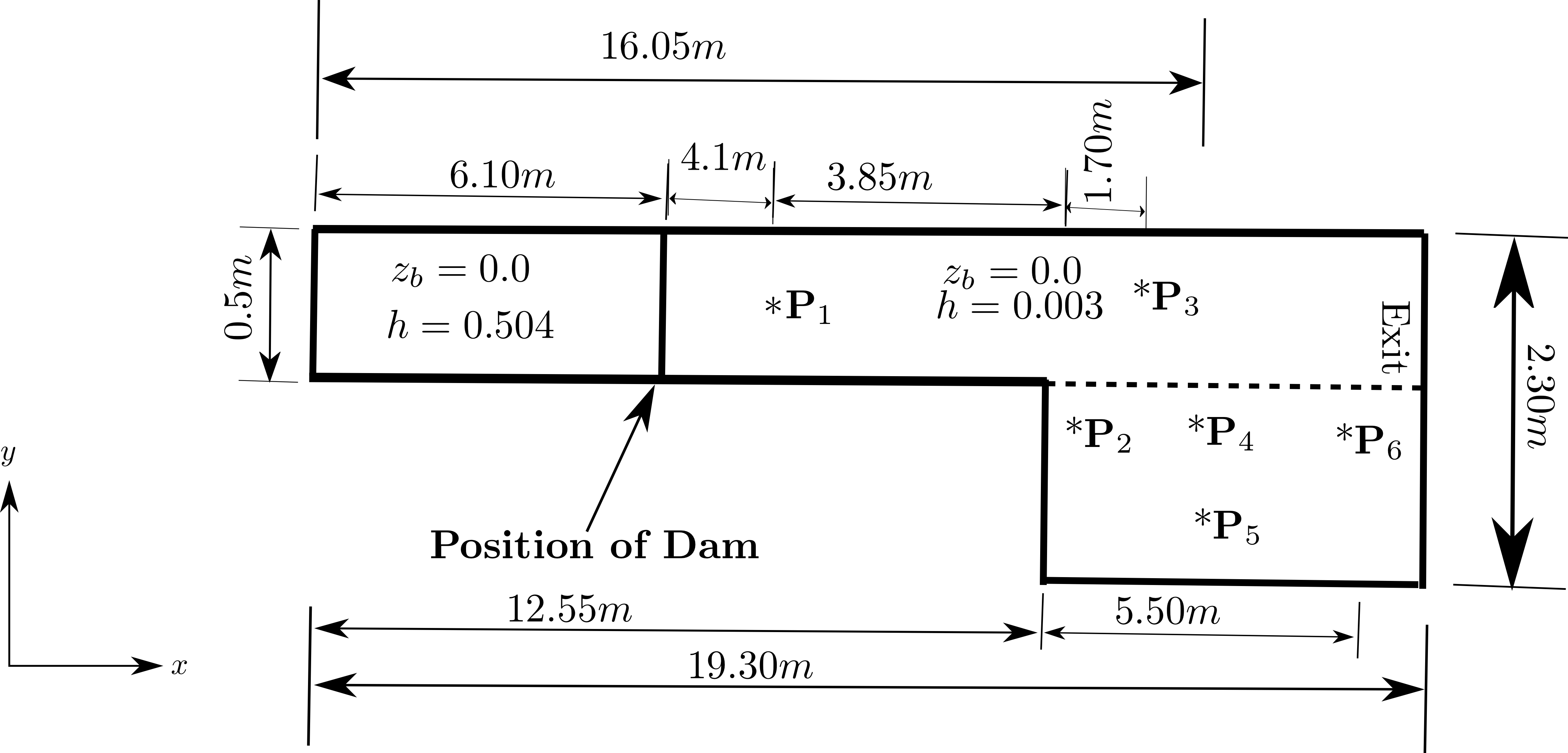
Refer to caption
Figure 8: Top view of Channel and Floodplain for river-flooding problem for test case 1

Here, a full 2D simulation was run with a grid of 193×2519325193\times 25 cells in the channel and 68×90689068\times 90 cells in the floodplain, while a simulation with the proposed method was run with a grid of 68×90689068\times 90 cells for the floodplain and 193×21932193\times 2 cells in the channel, and the simulation using the FBM was also run with a grid of 68×90689068\times 90 cells in floodplain and 193×11931193\times 1 in the channel, see table 1.

Channel Grid Floodplain Grid No. of time steps Processor time (in seconds)
Full 2D 193×2519325193\times 25 68×90689068\times 90 3,669 3,110.31
HCM 193×21932193\times 2 68×90689068\times 90 2,616 1,420.4
FBM 193×11931193\times 1 68×90689068\times 90 2,592 1,311.26
Table 1: Grid cells, simulation times and number of time steps

Figure 9 displays the free surface elevation for the three simulation methods. We can see that both the proposed method and the FBM capture the behaviour of the full 2D simulation, and from the right end of the channel, one can also see that the proposed method approximates the full 2D result better than the FBM. This is more obvious in figure 10, in which the time evolution of the free surface elevation at the probe points (indicated in figure 8), are plotted for all the simulation methods. Furthermore, figure 11 displays the plots of the time evolution of the x𝑥x- and y𝑦y- velocity components at selected probe points. One can see that the HCM performs better than the FBM at the indicated points. Of particular interest is the y𝑦y-velocity component at the probe point, P3subscript𝑃3P_{3} which is located within the channel. We can see that while the FBM wrongly computed a zero y𝑦y-velocity all the time, the HCM computed the correct none-zero values with very good accuracy. It is thus very clear that the proposed method, HCM significantly outperforms the FBM for this test case.

In terms of efficiency, as shown in table 1, the full 2D simulation took 3,669 time steps and 3,100.31 seconds to complete this simulation while the coupling methods took less number of time steps and more than 50% reduced time to complete the same simulation. With the above observations, we conclude that it is possible to efficiently use coupling methods instead of full 2D simulation, and that the proposed method is capable of reproducing the full 2D solutions with greater accuracy than the FBM.

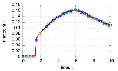
Refer to caption
Figure 9: Comparison of the final free surface elevation after ten seconds for test 1.
Refer to caption
Refer to caption
Refer to caption
Refer to caption
Refer to caption
Refer to caption
Refer to caption
Figure 10: Test 1 : Comparison of time evolution of the free surface elevation, η𝜂\eta at the probe points indicated in figure 8.
Refer to caption
Refer to caption
Refer to caption
Refer to caption
Refer to caption
Refer to caption
Refer to caption
Refer to caption
Refer to caption
Figure 11: Time evolution of the x𝑥x-velocity (left column) and y𝑦y-velocity (right column) at the indicated selected probe points for test case 1.

5.2 Test case 2 : Channel Flow into Elevated 2D Floodplain

This test case involves the same channel as in the previous example but connected to an elevated floodplain located in the region 10.5x16.010.5𝑥16.010.5\leq x\leq 16.0 (see figure 12). The channel bed is flat and the floodplain bed is 0.5 meters high. The initial condition is the following.

H(x,y,0)={1.5, if x8.5,y1.8,0.7, if x>8.5,y1.8,0.2, if 10.5x16.0,0y1.8,𝐻𝑥𝑦0cases1.5formulae-sequence if 𝑥8.5𝑦1.80.7formulae-sequence if 𝑥8.5𝑦1.80.2formulae-sequence if 10.5𝑥16.00𝑦1.8\displaystyle H(x,y,0)=\begin{cases}1.5,&\mbox{ if }x\leq 8.5,\quad y\geq 1.8,\\ 0.7,&\mbox{ if }x>8.5,\quad y\geq 1.8,\\ 0.2,&\mbox{ if }10.5\leq x\leq 16.0,\quad 0\leq y\leq 1.8,\end{cases} (84)
u(x,y,0)=v(x,y,0)=0.𝑢𝑥𝑦0𝑣𝑥𝑦00\displaystyle u(x,y,0)=v(x,y,0)=0. (85)

The manning coefficient for both channel and floodplain is taken as 0.009s/m1/3𝑠superscript𝑚13s/m^{1/3} the boundaries are only open at the sides indicated "exit" in figure 12, others are closed. Just like the previous test case, here nine probe points, P1P9subscript𝑃1subscript𝑃9P_{1}-P_{9} are identified, see figure 12.

Refer to caption
Figure 12: Top view of Channel and Floodplain for test case 2 showing the floodplain region in (x,y)[10.5,16.0]×[0,1.8]𝑥𝑦10.516.001.8(x,y)\in[10.5,16.0]\times[0,1.8] and the channel region in (x,y)[0,19.3]×[1.8,2.3]𝑥𝑦019.31.82.3(x,y)\in[0,19.3]\times[1.8,2.3].

All the methods solved this problem with a grid of 55×90559055\times 90 cells in the floodplain while the channel consists of 193×2519325193\times 25, 193×21932193\times 2 and 193×11931193\times 1 cells for the full 2D, the HCM and the FBM respectively, see table 2. The simulation was run for ten seconds. Figures 13 and 14 show the free surface elevation and velocity magnitude after the last time step for each method. It can be seen that the HCM provides a better approximation of the full 2D results than the FBM. As a further validation of this claim, the time evolution of the free surface elevation is plotted in figures 15, while those of the x𝑥x-velocity and y𝑦y-velocity components are plotted in figure 16 for selected probe points. It can be seen that the horizontal coupling method is more accurate than the FBM at the points for all flow quantities and almost all the time. Again, the HCM really captures the flow structure of the full 2D simulation. This proves the accuracy of the proposed methods over the FBM for this test case.

Channel Grid Floodplain Grid No. of time steps Processor time (in seconds)
Full 2D 193×2519325193\times 25 55×90559055\times 90 4,963 4,100.47
HCM 193×21932193\times 2 55×90559055\times 90 3,235 1,710.36
FBM 193×11931193\times 1 55×90559055\times 90 3,178 1,555.08
Table 2: Grid cells, simulation times and number of time steps : Test 2

For efficiency, we see from the processing time in table 2 that the FBM is very efficient but not very accurate while the horizontal coupling method is both very efficient and also has good accuracy.
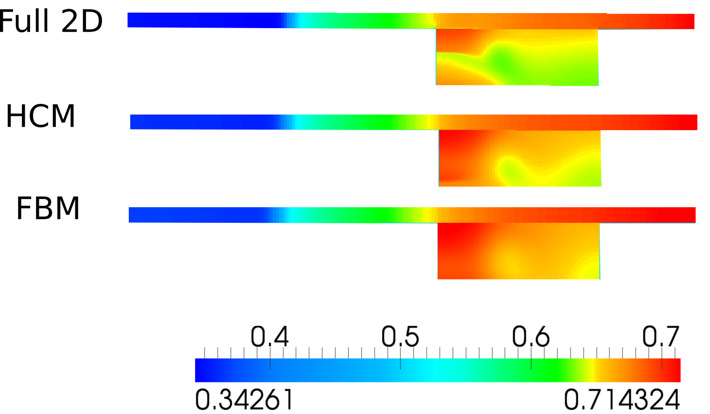
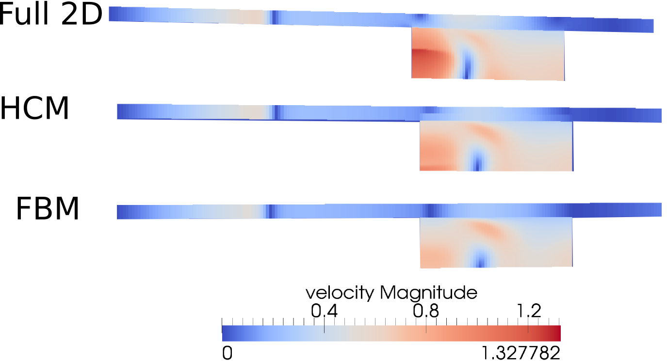
Refer to caption
Figure 13: Comparison of free surface elevation for the different methods after the last time step: Test 2
Refer to caption
Figure 14: Comparison of velocity magnitude for the different methods after the last time step: Test 2
Refer to caption
Refer to caption
Refer to caption
Refer to caption
Refer to caption
Refer to caption
Refer to caption
Refer to caption
Refer to caption
Figure 15: Comparison of time evolution of water height at probe points : Test 2
Refer to caption
Refer to caption
Refer to caption
Refer to caption
Refer to caption
Refer to caption
Refer to caption
Refer to caption
Refer to caption
Figure 16: Time evolution of x𝑥x-velocity (left column) and y𝑦y-velocity (right column) at the indicated selected probe points for test case 2.

5.3 Test case 3 : Flooding of an initially dry floodplain
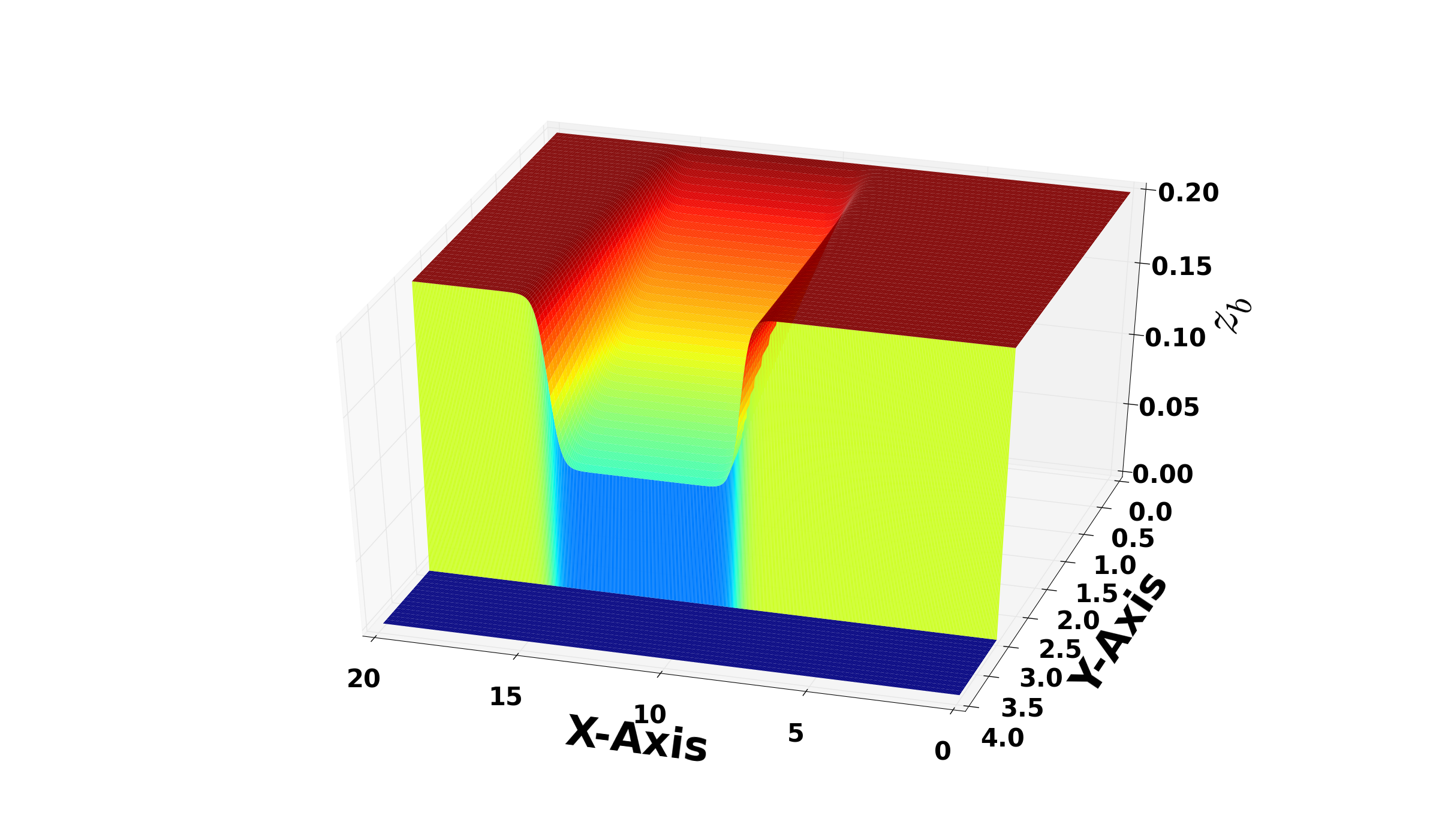
Refer to caption
(a) Bottom elevation, zb(x,y)subscript𝑧𝑏𝑥𝑦z_{b}(x,y) in Ω2superscriptΩ2\Omega^{2}
Refer to caption
(b) Channel Wall Elevation, zbw(x)superscriptsubscript𝑧𝑏𝑤𝑥z_{b}^{w}(x)
Figure 17: The 2D bed elevation and channel wall elevation for test 3

The final test case involves the overflowing of a channel onto an initially dry floodplain. Both the channel and the floodplain are located in the 2D2𝐷2D domain, [0,20]×[0,4]02004[0,20]\times[0,4]. The channel occupies the region, [0,20]×[yc,4]020subscript𝑦𝑐4[0,20]\times[y_{c},4] with flat bottom, Zb(x)=0subscript𝑍𝑏𝑥0Z_{b}(x)=0, while the floodplain occupies the rest of the domain, [0,20]×[0,yc]0200subscript𝑦𝑐[0,20]\times[0,y_{c}], where yc=3subscript𝑦𝑐3y_{c}=3. The bottom topography of the entire domain is the following

zb(x,y)={Zb(x)=0, if yyc,0.2+zbw(x)0.2ycy, otherwise ,,subscript𝑧𝑏𝑥𝑦casessubscript𝑍𝑏𝑥0 if 𝑦subscript𝑦𝑐0.2superscriptsubscript𝑧𝑏𝑤𝑥0.2subscript𝑦𝑐𝑦 otherwise \displaystyle z_{b}(x,y)=\begin{cases}Z_{b}(x)=0,&\mbox{ if }y\geq y_{c},\\ 0.2+\frac{z_{b}^{w}(x)-0.2}{y_{c}}y,&\mbox{ otherwise },\end{cases}, (86)

where

zbw(x)={0.06tanh(3(x9))+0.14, if x10.5,0.06tanh(3(x15.5))+0.14, otherwisesuperscriptsubscript𝑧𝑏𝑤𝑥cases0.063𝑥90.14 if 𝑥10.50.063𝑥15.50.14 otherwise\displaystyle z_{b}^{w}(x)=\begin{cases}-0.06\tanh(3(x-9))+0.14,&\mbox{ if }x\leq 10.5,\\ 0.06\tanh(3(x-15.5))+0.14,&\mbox{ otherwise }\end{cases} (87)

is the elevation of the channel wall, see figures 17(a) and 17(b) for the plots of zb(x,y)subscript𝑧𝑏𝑥𝑦z_{b}(x,y) and zbw(x)superscriptsubscript𝑧𝑏𝑤𝑥z_{b}^{w}(x).

The initial condition consists of stationary water of depth, 0.08 meters in the channel and dry floodplain. The boundary conditions are time-dependent water depth at the left boundary of the channel and zero velocity at the right channel boundary, namely

H(0,y,t)={hb(t), if t4a,hb(4a), if t>4a,𝐻0𝑦𝑡casessubscript𝑏𝑡 if 𝑡4𝑎subscript𝑏4𝑎 if 𝑡4𝑎\displaystyle H(0,y,t)=\begin{cases}h_{b}(t),&\mbox{ if }t\leq 4a,\\ h_{b}(4a),&\mbox{ if }t>4a,\end{cases} (88)
for yyc.for 𝑦subscript𝑦𝑐\displaystyle\mbox{ for }y\geq y_{c}.
u(20,y,t)=0.0, for all t0,yyc,formulae-sequence𝑢20𝑦𝑡0.0formulae-sequence for all 𝑡0𝑦subscript𝑦𝑐\displaystyle u(20,y,t)=0.0,\mbox{ for all }t\geq 0,y\geq y_{c}, (89)

where

hb(t)=η0+r+rsin((ta)π2a),subscript𝑏𝑡subscript𝜂0𝑟𝑟𝑡𝑎𝜋2𝑎h_{b}(t)=\eta_{0}+r+r\sin\bigg{(}\frac{(t-a)\pi}{2a}\bigg{)}, (90)

where a=10𝑎10a=10 and r=0.025𝑟0.025r=0.025. η0=0.08subscript𝜂00.08\eta_{0}=0.08 is a constant initial free-surface elevation inside the channel. The remaining boundaries are closed and the manning coefficients are the same as used in the previous cases. The following probe points are chosen, P1=(2.5,3.5)subscript𝑃12.53.5P_{1}=(2.5,3.5), P2=(4.0,3.8)subscript𝑃24.03.8P_{2}=(4.0,3.8), P3=(7.0,3.3)subscript𝑃37.03.3P_{3}=(7.0,3.3), P4=(10.0,3.4)subscript𝑃410.03.4P_{4}=(10.0,3.4), P5=(11,3.5)subscript𝑃5113.5P_{5}=(11,3.5), P6=(12,3.3)subscript𝑃6123.3P_{6}=(12,3.3), P7=(14,3.4)subscript𝑃7143.4P_{7}=(14,3.4), P8=(16,3.5)subscript𝑃8163.5P_{8}=(16,3.5), P9=(17.3,3.5)subscript𝑃917.33.5P_{9}=(17.3,3.5), P10=(19,3.5)subscript𝑃10193.5P_{10}=(19,3.5), P11=(12,2.8)subscript𝑃11122.8P_{11}=(12,2.8), P12=(13,2.8)subscript𝑃12132.8P_{12}=(13,2.8), P13=(12,2.5)subscript𝑃13122.5P_{13}=(12,2.5), P14=(12,2.0)subscript𝑃14122.0P_{14}=(12,2.0) and P15=(13.0,1.0)subscript𝑃1513.01.0P_{15}=(13.0,1.0).

Table 3 shows the domain discritization for both the channel and the floodplain for each method being discussed. As before, all methods use the same grid for the floodplain but different grids for the channel. This problem was simulated for t=100𝑡100t=100 seconds. We report, in figures 18 - 21, the results of the simulation after 40 seconds and in figures 22 and 23, we report the results at selected probe points throughout the duration of the simulation.

As can been seen from the pictures, both coupling methods provide very good approximation of full 2D simulation results for both the free surface elevation (figure 18), the velocity components (figures 19 and 20) and the velocity magnitude (figure 21) for this test case. And in terms of accuracy of y-velocity component, the HCM provides better approximations as can be seen in figure 20.

Channel Grid Floodplain Grid
Full 2D 600×3060030600\times 30 600×9060090600\times 90
HCM 600×26002600\times 2 600×9060090600\times 90
FBM 600×16001600\times 1 600×9060090600\times 90
Table 3: Grid cells, simulation times and number of time steps : Test 3
Refer to caption
Figure 18: Visualisation of free surface elevation after t=40𝑡40t=40 for test case 3. The x𝑥x-axis is from left to right, while the y𝑦y-axis is from the bottom to the top.
Refer to caption
Figure 19: Visualisation of x𝑥x-velocity after t=40s𝑡40𝑠t=40s for test case 3. The x𝑥x-axis is from left to right, while the y𝑦y-axis is from the bottom to the top.
Refer to caption
Figure 20: Visualisation of y𝑦y-velocity after t=40s𝑡40𝑠t=40s for test case 3. The x𝑥x-axis is from left to right, while the y𝑦y-axis is from the bottom to the top.
Refer to caption
Figure 21: Visualisation of velocity magnitude after t=40s𝑡40𝑠t=40s for test case 3. The x𝑥x-axis is from left to right, while the y𝑦y-axis is from the bottom to the top.
Refer to caption
Refer to caption
Refer to caption
Refer to caption
Refer to caption
Refer to caption
Refer to caption
Refer to caption
Refer to caption
Refer to caption
Refer to caption
Refer to caption
Refer to caption
Figure 22: Time variation of water depth H𝐻H (left column), x𝑥x-velocity component (middle column) and y𝑦y-velocity component (right column) at the indicated probe points within the channel for test case 3. Each row corresponds to one probe point.
Refer to caption
Refer to caption
Refer to caption
Refer to caption
Refer to caption
Refer to caption
Refer to caption
Refer to caption
Refer to caption
Refer to caption
Refer to caption
Refer to caption
Refer to caption
Figure 23: Time variation of water depth H𝐻H (left column), x𝑥x-velocity component (middle column) and y𝑦y-velocity component (right column) at the indicated probe points in the floodplain for test case 3. Each row corresponds to one probe point.

To further understand the results of the simulations, the time evolution of the flow quantities at the probe points, P1P15subscript𝑃1subscript𝑃15P_{1}-P_{15} have been examined. Here we report the results at the probe points P1,P4,P5subscript𝑃1subscript𝑃4subscript𝑃5P_{1},P_{4},P_{5} and P6subscript𝑃6P_{6} which are in the channel and the points, P11,P12,P13subscript𝑃11subscript𝑃12subscript𝑃13P_{11},P_{12},P_{13} and P14subscript𝑃14P_{14} in the floodplain. Figures 22 and 23 show the results for the selected points in the channel and floodplain respectively. In each figure, the left column displays the water depth, the second (middle) column shows the xlimit-from𝑥x-component of velocity, while the third(right) column shows the ylimit-from𝑦y-component of velocity.

From figure 22, we can see that both coupling methods provide very good approximation of the results of the full 2D simulations, especially for the water depth and xlimit-from𝑥x-component of velocity. However, only the HCM is able to compute the variation in the ylimit-from𝑦y-velocity and it does so with very good accuracy, see P4,P5,P6subscript𝑃4subscript𝑃5subscript𝑃6P_{4},P_{5},P_{6} in figure 22. This further verifies the ability of of the HCM to compute the lateral discharges within the channel.

From figure 23, we also see that for the points in the floodplain, the coupling methods computed very good approximations of results of the full 2D simulation with the HCM computing more accurate results especially for the ylimit-from𝑦y-velocity. This figure also verify the no-numerical flooding property of the methods. That is, the floodplain initially remained dry until the time when water height rose above the channel banks. This is the reason why, for all points in the floodplain, the water depth and velocity remained at zero for the first several seconds of the simulation. Another thing to note is that due to the time-dependent boundary condition for this problem, water flowed onto the floodplain and after some time the water level in the channel decreased, hence the water in the floodplain drains back into the channel leaving the floodplain dry again. The coupling methods truly capture this phenomenon as one can see in figure 23 where the water depth and velocity return to zero towards the end of the simulation and remain at zero throughout the rest of the simulation. This is true for all the points in the floodplain, even those not reported here.

6 Conclusion

A horizontal coupling method has been proposed, implemented and tested in this paper. It presents a strategy to overcome the difficulty in computing the channel lateral discharges, circumvent the 1D assumption on the channel lateral discharge during flooding and propose a variant of the coupling term of [12] without the use of or imposing any restriction on the channel width variation. Numerical experiments show that the method computes adequate results. Particularly, the channel lateral discharges are properly computed without adopting complicated/iterative procedures. Finally, we note that for all the numerical test cases considered in this paper, the HCM would coincide with the FBM if the lateral discharges were not computed in the HCM. Therefore, the improved solution observed in the HCM over the FBM, for these test cases, is a result of the lateral discharges that are computed in the HCM. We, therefore, conclude that properly computing and restoring the channel lateral discharge, improves the quality of the computed solution and this can be done without introducing much computational overhead.

Acknowledgement

We are grateful to the Petroleum Technology Development Fund (PTDF), Nigeria for funding this study and to the Centre for Scientific Computing, University of Warwick for providing the computing resources.

References

  • [1] E. Audusse, F. Bouchut, M. Bristeau, R. Klein, and B. Perthame. A fast and stable well-balanced scheme with hydrostatic reconstruction for shallow water flows. SIAM Journal Scientific Computing, 25:2050–2065, 2004.
  • [2] E. Bladé, M. Gómez-Valentín, J. Dolz, J. Aragón-Hernández, G. Corestein, and M. Sánchez-Juny. Integration of 1d and 2d finite volume schemes for computations of water flow in natural channels. Advances in Water Resources, 42:17–29, 2012.
  • [3] F. Bouchut. Efficient Numerical Finite Volume Schemes for Shallow Water Models. Elsevier, 2007.
  • [4] Y. Chen, Z. Wang, Z. Liu, and D. Zhu. 1d-2d coupled numerical model for shallow-water flows. Journal of Hydraulic Engineering., 138:122–132, 2012.
  • [5] J. A. Cunge, F. M. Holly, and A. Verwey. Practical aspects of computational river hydraulics. Pitman publishing, 1980.
  • [6] E. D. Fernandez-Nieto, J. Marin, and J. Monnier. Coupling superposed 1d and 2d shallow-water models: Source terms in finite volume schemes. Computers & Fluids, 39(6):1070–1082, 2010.
  • [7] R. Ghostine, I. Hoteit, J. Vazquez, A. Terfous, A. Ghenaim, and R. Mose. Comparison between a coupled 1d-2d model and a fully 2d model for supercritical flow simulation in crossroads. Journal of Hydraulic Research, 53(2):274–281, 2015.
  • [8] N. Goutal, M. Parisot, and F. Zaoui. A 2d reconstruction for the transverse coupling of shallow water models. International Journal for Numerical Methods in Fluids, 75(11):775–799, 2014.
  • [9] A. Harten, P. D. Lax, and B. Van Leer. On upstream differencing and godunov-type schemes for hyperbolic conservation laws. SIAM review, 25(1):35–61, 1983.
  • [10] D. Lannes. Water Waves Problem. Mathematical Analysis and Asymptotics. AMS, 2013.
  • [11] I. MacDonald. Analysis and computation of steady open channel flow. PhD thesis, University of Reading Reading, UK, 1996.
  • [12] J. Marin and J. Monnier. Superposition of local zoom models and simultaneous calibration for 1d-2d shallow water flows. Mathematics and Computers in Simulation, 80(3):547–560, 2009.
  • [13] M. Morales-Hernández. Efficient Explicit Finite Volume Schemes for the shallow water equations with solute transport. PhD thesis, Universidad Zaragoza, 2014.
  • [14] M. Morales-Hernández, P. García-Navarro, J. Burguete, and P. Brufau. A conservative strategy to couple 1d and 2d models for shallow water flow simulation. Computers & Fluids, 81:26–44, 2013.
  • [15] M. Morales-Hernández, P. García-Navarro, and J. Murillo. A large time step 1d upwind explicit scheme (cfl> 1): Application to shallow water equations. Journal of Computational Physics, 231(19):6532–6557, 2012.
  • [16] M. Morales-Hernández, G. Petaccia, P. Brufau, and P. García-Navarro. Conservative 1d–2d coupled numerical strategies applied to river flooding: The tiber (rome). Applied Mathematical Modelling, 40(3):2087–2105, 2016.
  • [17] C. Nwaigwe. Coupling Methods for 2D/1D Shallow Water Flow Models for Flood Simulations. PhD thesis, University of Warwick, United Kingdom, 2016.
  • [18] S. D. Seyoun, Z. Vojinovic, R. K. Price, and S. Weesakul. Coupled 1d and noninertia 2d flood inundation model for simulation of urban flooding. Journal of Hydraulic Engineering, 138:23–34, 2012.
  • [19] E. F. Toro. Riemann solvers and numerical methods for fluid dynamics: a practical introduction. Springer Science & Business Media, 1999.
  • [20] E. F. Toro. Shock Capturing Methods For Free-surface Flows. Wiley, 2001.
  • [21] T. Viseu, A. Franco, and A. B. de Almeida. Numerical and computational results of the 2-d biplan model. In 4th Meeting of the Working Group on Dam-Break Modelling (1st CADAM Meeting), 1999.