Discrete affine Gaussian receptive fieldsTony Lindeberg
Discrete approximations of the affine Gaussian derivative model for visual receptive fields††thanks: \fundingThe support from the Swedish Research Council (contract 2014-4083) is gratefully acknowledged.
Abstract
The affine Gaussian derivative model can in several respects be regarded as a canonical model for receptive fields over a spatial image domain: (i) it can be derived by necessity from scale-space axioms that reflect structural properties of the world, (ii) it constitutes an excellent model for the receptive fields of simple cells in the primary visual cortex and (iii) it is covariant under affine image deformations, which enables more accurate modelling of image measurements under the local image deformations caused by the perspective mapping, compared to the more commonly used Gaussian derivative model based on derivatives of the rotationally symmetric Gaussian kernel.
This paper presents a theory for discretizing the affine Gaussian scale-space concept underlying the affine Gaussian derivative model, so that scale-space properties hold also for the discrete implementation.
Two ways of discretizing spatial smoothing with affine Gaussian kernels are presented: (i) by solving semi-discretized affine diffusion equation, which has been derived by necessity from the requirements of a semi-group structure over scale as parameterized by a family of spatial covariance matrices and obeying non-creation of new structures from any finer to any coarser scale in terms of non-enhancement of local extrema and (ii) approximating these semi-discrete affine receptive fields by parameterized families of -kernels as obtained from an additional discretization along the scale direction. The latter discrete approach can be optionally complemented by spatial subsampling at coarser scales, leading to the notion of affine hybrid pyramids.
For the first approach, we show how the solutions can be computed reasonably efficiently from a closed form expression for the Fourier transform, and analyse how a remaining degree of freedom in the theory can be explored to ensure a positive discretization and optionally achieve higher-order discrete approximation of the angular dependency of the discrete affine Gaussian receptive fields. For the second approach, we analyse how the step length in the scale direction can be determined, given the requirements of a positive discretization and other scale-space properties.
We do also show how discrete directional derivative approximations can be efficiently implemented to approximate affine Gaussian derivatives. Using these theoretical results, we outline hybrid architectures for discrete approximations of affine covariant receptive field families, to be used as a first processing layer for affine covariant and affine invariant visual operations at higher levels.
keywords:
scale space, scale, affine, receptive field, Gaussian kernel, discrete, spatial, spatio-chromatic, double-opponent, feature detection, computer vision.65D18, 65D19, 68U10
1 Introduction
A basic fact when interpreting image information is that a pointwise measurement of the image intensity at a single image point does usually not carry any relevant information, since it is dependent on external and unknown illumination. The essential information is instead mediated by the relations between the image intensities at neighbouring points. To handle this issue, the notion of receptive fields has been developed in both biological vision and computer vision, by performing local image measurements over neighbourhoods of different spatial extent (Hubel and Wiesel [29, 30]; DeAngelis et al. [15, 14]; Conway and Livingstone [8]; Johnson et al. [32]; Shapley and Hawken et al. [66]; Koenderink and van Doorn [34, 35]; Young et al. [81, 82]; Lindeberg [44, 49, 50]; Schiele and Crowley [64]; Lowe [55]; Dalal and Triggs [13]; Serre et al. [65]; Bay et al. [4]; Burghouts and Geusebroek [6]; van de Sande et al. [62]; Tola et al. [71]; Linde and Lindeberg [41]; Larsen et al. [37]; Krizhevsky et al. [36]; Simonyan and Zisserman [67]; Szegedy et al. [70]; He et al. [27]).
A fundamental problem in this context concerns what shapes of receptive field profiles are meaningful. Would any shape of the receptive field do? This problem has been addressed from an axiomatical viewpoint in the area of scale-space theory, by deriving families of receptive fields that obey scale-space axioms that reflect structural properties of the world. Over an isotropic spatial domain, arguments and axiomatic derivations by several researchers have shown that the rotationally symmetric Gaussian kernel and Gaussian derivatives derived from it constitute a canonical family of kernels to model spatial receptive fields (Iijima [31]; Koenderink [33]; Koenderink and van Doorn [34, 35]; Lindeberg [44, 48]; Florack [22]; ter Haar Romeny [25]; Weickert et al. [80]). Such Gaussian derivatives can in turn be used as primitives for expressing a large class of visual modules in computer vision, including feature detection, feature classification, surface shape, image matching and object recognition.
The underlying assumption about spatial isotropy that underlies the part of the scale-space theory that leads to receptive fields based on rotational symmetric Gaussian kernels is, however, neither necessary nor always desirable. For images of objects that are subject to variations in the viewing direction, the perspective mapping leads to non-isotropic perspective transformations that are not within the group of image transformations covered by rotationally symmetric Gaussian kernels. If we locally at every image point approximate the non-linear perspective mapping by its derivative, then the effect of the perspective mapping can for locally smooth surfaces to first order of approximation be approximated by local affine image deformations. If we would like to base a vision system on a receptive field model that is closed under such affine transformations, we should therefore replace the rotationally symmetric Gaussian kernels by affine Gaussian kernels (Lindeberg [44]; Lindeberg and Gårding [53, 54]). Interestingly, the family of affine Gaussian kernel and affine Gaussian derivatives can also be uniquely derived from basic scale-space axioms that reflect structural properties of the world in combination with a requirement about internal consistency between image representations at multiple spatial scales (Lindeberg [48]).
The subject of this article is to address the problem of how to discretize receptive fields based on affine Gaussian derivatives, while preserving scale-space properties also in a discrete sense. This work constitutes a continuation of a previously developed scale-space theory for discrete signals and images (Lindeberg [42, 44, 43]), which was conceptually extended to a discrete affine scale-space in a conference publication (Lindeberg [45]), while leaving out several details that are needed when implementing the theory in practice. The work is also closely related to other work on discretizing scale-space operations as done by Deriche [16], Weickert et al. [77, 79], van Vliet et al. [75], Wang [76], Florack [21], Almansa and Lindeberg [1], Lim and Stiehl [40], Geusebroek et al. [23], Farid and Simoncelli [18], Bouma et al. [5], Dollár et al. [17], Tschirsich and Kuijper [72], Slavík and Stehlík [69], Lindeberg [51] and others.
We will show that by axiomatic arguments it is possible to derive a three-parameter family of semi-discrete affine Gaussian receptive fields, where the receptive fields are discretized over image space, while being continuous over scale as parameterized by a family of spatial covariance matrices that represent receptive fields of different sizes and orientations in the image domain as well as different eccentricities in terms of the ratio between the eigenvalues of the spatial covariance matrix. The resulting family of discrete affine Gaussian receptive fields obeys discrete analogues of several of the properties that define the uniqueness of the continuous affine Gaussian kernel over a continuous spatial domain.
For both theoretical and practical purposes, we will show that these receptive fields can up to numerical errors in an actual implementation be computed exactly in terms of a closed-form expression of the Fourier transform, thus without explicit need for solving the PDE that describes the evolution over scale using approximate methods. If convolution by FFT can be regarded sufficiently computationally efficient, then this discretization method gives the numerically most accurate approximation of the continuous affine scale-space concept, and also allowing for a full transfer of the underlying scale-space properties to the discrete implementation.
It will also be shown that if this theory is additionally discretized over scale, then this leads to families of compact -kernels that can be interpreted as discretizations of affine Gaussian kernels, and which are to be applied repeatedly. Such kernels can be efficiently implemented on parallel architectures such as GPUs. This model will be developed in two versions: (i) a conceptually simpler model that preserves the same resolution at all levels of scale and (ii) a hybrid pyramid model that enables higher computational efficiency by combining the iterative spatial smoothing operations with subsampling stages at coarser levels of scale, implying that less computations will be needed because of the resulting lower number of image pixels at coarser resolutions and the ability to take larger scale steps.
The latter type of model does specifically have an interesting structural relationship to recent developments in deep learning, where deep networks, such as VGG-Net (Simonyan and Zisserman [67]) and ResNet (He et al. [27]), are based on automated learning of compact kernels that are applied in a repeated layered structure to the image data.
With the theory presented in this paper, we aim at opening up for relating such kernels to scale-space operations, with the possibilities of building closer links between the empirical developments in deep learning and axiomatically derived scale-space theory with its in turn close relations to receptive fields in biological vision. A long term goal is to open up for hybrid architectures that combine ideas and concepts from scale-space theory, pyramid representation and deep learning, to allow for cross-fertilization between these areas.
A specific aim is to replace the training of the earliest layers in deep networks by theoretically derived scale-space filters that obey the algebra of affine Gaussian receptive fields, to enable affine covariance of the deep network, to in turn enable provably affine invariant recognition methods based on deep learning that are able to work more robustly under local image deformations caused by perspective effects.
Specifically, we propose that the computational architectures developed in this paper, in terms of directional derivatives of different orders of spatial differentiation, in different orientations in image space and over variations in the sizes and the shapes (eccentricities) of affine Gaussian kernels, with their conceptually very large similarities to the spatial receptive fields of simple cells in the primary visual cortex (V1), can be used as the first layers of input to both classical type computer vision/image analysis methods and deep networks.
1.1 Structure of this article
This article is organized as follows: Section 2 gives an overview of the affine Gaussian derivative model for spatial receptive fields, with its properties of: (i) being determined by necessity from scale-space axioms that reflect structural properties of the world, (ii) being able to handle local perspective image deformations in a covariant manner and (iii) having close similarities to receptive fields in biological vision.
Section 3 gives an overview of basic approaches for discretizing the continuous model for affine Gaussian receptive fields over a spatial domain, with specific mention of the different types of properties that different spatial discretizations lead to. Section 4 then describes a genuine discrete theory for defining discrete analogues of affine Gaussian receptive fields in such a way that the discrete receptive fields exactly obey discrete analogues of several of the special properties that the continuous affine Gaussian kernels obey.
Section 5 gives a deeper treatment of this topic for the specific case of a two-dimensional image domain, based on a semi-discrete affine diffusion equation that defines semi-discrete affine Gaussian kernels over a discretized spatial image domain, while maintaining a continuum of affine scale-space representations over a three-parameter family of affine covariance matrices that represent the shapes of spatial kernels with different sizes and orientations in the image domain and with different eccentricities in terms of the ratios between the eigenvalues of the covariance matrix.
Section 6 then discretizes the above semi-discrete theory additionally over scale, in terms of a discrete set of spatial covariance matrices for which receptive fields are to be computed, and shows that this leads to families of compact -kernels, which allow for efficient implementation on parallel architectures such as GPUs.
Section B in the appendix additionally combines that theory with the notion of pyramid representation, and shows how families of affine hybrid pyramid representations can be defined from the discrete approach, with the additional constraint that receptive field responses at coarser spatial scales may be represented at coarser spatial resolution, to reduce the computational work and the memory requirements.
Section 7 shows how scale-normalized derivatives can be defined for the presented discrete approaches. Finally, Section 8 gives a summary and discussion about some of the main results and describes how the presented theory opens up for different types of architectures for affine covariant and affine invariant visual receptive fields.
To not load the main flow of article with too much technical material, we have put the axiomatic derivation of the discrete affine scale-space concept, which constitutes the theoretical foundation for the treatment in Section 4 as well as the later sections that build upon this material, in Appendix A. A condensed summary of the necessary material resulting from the axiomatic treatment is given in Section 4.1.
2 The affine Gaussian derivative model for receptive fields over a continuous image domain
This section gives an overview of the affine Gaussian derivative model regarding: (i) its axiomatic derivation from assumptions that reflect structural properties of the world in combination with internal consistency requirements between image representations at different scales, (ii) how it leads to families of spatial and spatio-chromatic receptive fields, (iii) its relations to receptive field profiles in biological vision and (iv) its affine covariance properties as highly desirable for computing receptive field responses under perspective image deformations. This material constitutes the theoretical and conceptual background for the genuine discrete theory that will be developed in Sections 4–7 and Appendix B.
2.1 Spatial affine Gaussian derivative based receptive fields
Let us assume that the spatial smoothing operation in a spatial scale-space representation should obey: (i) linearity, (ii) spatial shift invariance, (iii) a semi-group structure over spatial scales and (iv) a requirement of not introducing new structures from finer to coarser scales formalized in terms of non-enhancement of local extrema, meaning that the value at a local maximum must not increase from finer to coarser scales and correspondingly the value at a local minimum must not decrease. Then, it can be shown that affine Gaussian kernels
| (1) |
are uniquely determined by necessity (Lindeberg [48]). Directional derivatives of these kernels do in turn constitute a canonical model for spatial receptive fields over a two-dimensional image domain (Lindeberg [49, 50]).
For the specific parameterization of the spatial covariance matrix , convolution with these kernels obeys the affine diffusion equation
| (2) |
with initial condition . Convolution with affine Gaussian kernels also obeys the cascade smoothing property
| (3) |
To parameterize the affine Gaussian kernels, let us in the two-dimensional case consider the covariance matrix determined by two eigenvalues , and one orientation . Then, the covariance matrix can be written
| (4) | ||||
|
 |
 |
 |
 |
 |
|---|---|---|---|---|---|
|
 |
 |
 |
 |
 |

|
 |
 |
 |
 |
 |
|
 |
 |
 |
 |
 |
|---|---|---|---|---|---|
|
 |
 |
 |
 |
 |
|
 |
 |
 |
 |
 |
|
 |
 |
 |
 |
 |
Correspondingly, we can for two orthogonal directions and aligned to the eigendirections of the spatial covariance matrix parameterize the directional derivative operators in these directions according to
| (5) |
This leads to the following canonical model for affine Gaussian receptive fields over a spatial domain (Lindeberg [48])
| (6) |
preferably with the angle in (5) and (6) chosen equal to the angle in (4).
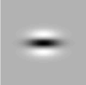
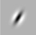
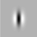
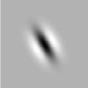
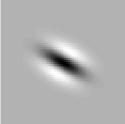
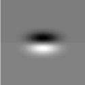
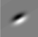
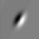
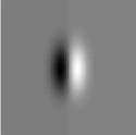
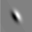
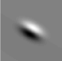
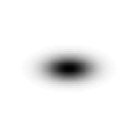
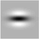
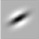
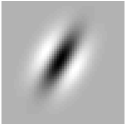
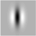
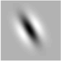
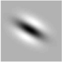
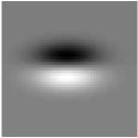
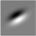
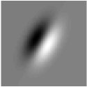
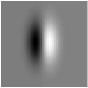
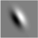
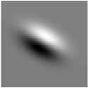
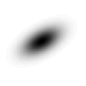
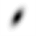
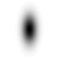
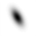
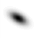
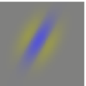
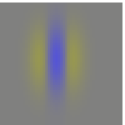
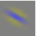
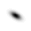
Figure 1 shows a few examples of affine Gaussian kernels and their directional derivatives up to order two for one combination of the two eigenvalues determined such that the ratio between the scale parameters in the two eigendirections of the covariance matrix is equal to two, with the scale parameters and expressed in terms of dimension .
2.2 Spatio-chromatic affine Gaussian derivative based receptive fields
Consider next the colour channels of colour-opponent space defined from an RGB colour representation (Hall et al. [26])
| (7) |
where represents the red/green colour-opponent channel and the yellow/blue colour-opponent channel, with yellow approximated by the average of the and channels and denoting the channel of pure intensity information.
Then, affine Gaussian colour-opponent receptive fields can be defined by applying affine Gaussian receptive fields of the form (6) to the colour-opponent channels :
| (8) | ||||
| (9) | ||||
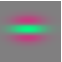
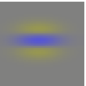
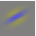
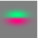
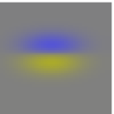
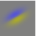
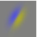
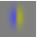
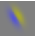
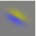
Figure 2 shows examples of such affine Gaussian spatio-chromatic receptive fields up to order two over red/green and yellow/blue colour-opponent space.
2.3 Relations to biological receptive fields
In the most ideal form of the affine Gaussian receptive field model, one should at any image point consider affine receptive fields as being present for all positive definite covariance matrices , as parameterized by their eigenvalues and and for all directions .
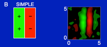
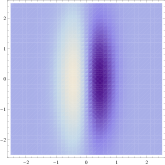
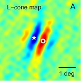
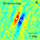
This model is proposed in Lindeberg [48, Section 6] [49, Section 6.3]) as a model for the spatial component of simple cells in the primary visual cortex (V1) and is in good agreement with neural cell recordings by DeAngelis et al. [15, 14] and Johnson et al. [32]. Figure 4 shows an example of the spatial dependency of a simple cell that can be well modelled by a first-order affine Gaussian derivative over image intensities. Figure 4 shows corresponding results for a color-opponent receptive field of a simple cell in V1 that can be modelled as a first-order affine Gaussian spatio-chromatic derivative over an R-G colour-opponent channel.
 |
 |
 |
 |
 |
 |
 |
2.4 Affine covariance
A theoretically very attractive property of the affine Gaussian model for spatial receptive fields is that this family of receptive fields is closed under affine transformations of the spatial image domain. If we consider two images and that with vector notation for the image coordinates and are related by an affine image deformation
| (10) |
and define corresponding scale-space representations according to
| (11) |
then these scale-space representations will be related according to (Lindeberg [44]; Lindeberg and Gårding [53, 54])
| (12) |
with and . In other words, given that an image is affine transformed into an image , it will always be possible to find a transformation between the spatial covariance matrices and in the two domains that makes it possible to match the corresponding derived internal representations and perfectly. If we in turn locally approximate the non-linear perspective image deformation between two images of the same scene by local affine deformations (first-order derivatives), then this means that it will to first-order of approximation be possible to match the receptive field responses computed from different views of the same scene.
This idea was originally proposed for reducing the shape distortions that arise when computing estimates of local surface orientation by shape-from-texture and shape-from-disparity-gradients (Lindeberg and Gårding [53, 54]) and has later been explored for image-based matching and recognition (Baumberg [3]; Schaffalitzky and Zisserman [63]; Sivic and Zisserman [68]; Mikolajczyk and Schmid [56]; Tuytelaars and van Gool [73]; Mikolajczyk et al. [57]; Lazebnik et al. [38]; Rothganger et al. [59]; Tuytelaars and Mikolajczyk [74]; Burghouts and Geusebroek [6]; Lia et al. [39]).
Similar ideas of affine invariance as underlying these approaches based on affine shape adaptation (Lindeberg [50]) have also been used for designing smoothing methods with a larger amount of smoothing along local image structures than across them (Weickert [78]; Almansa and Lindeberg [1]), for performing affine invariant segmentation (Ballester and González [2]; Rothganger et al. [60]), for constructing affine SIFT descriptors (Morel and Yu [58, 83]; Sadek et al. [61]), for affine invariant tracking (Giannarou et al. [24]), for formulating affine covariant metrics (Fedorov et al. [20]) and for affine invariant inpainting (Fedorov et al. [19]).
When implementing such affine covariance or affine invariance in practice, there are two main approaches to follow, either (i) by adapting the shape of the affine Gaussian kernel to the local image structure as proposed in the affine shape adaptation methodology proposed in (Lindeberg and Gårding [53, 54]) or (ii) by computing receptive field responses for all affine covariance matrices alternatively for some sparse sampling of the resulting family of receptive fields.
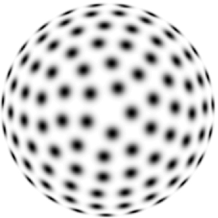
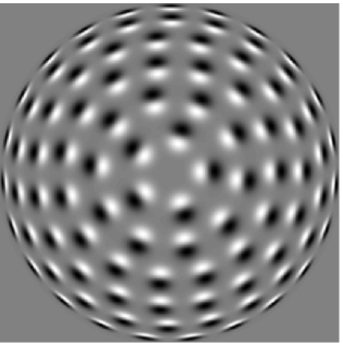
Figure 5 shows the resulting distributions of affine Gaussian receptive fields of different orientations and degrees of orientation as they arise from local linearizations of the perspective projection model, if we assume that (i) the set of surface directions in the world is on average uniformly distributed in the world and that (ii) the distributions of the local surface patterns on these object surfaces are in turn without dominant directional bias and uncoupled to the orientations of the local surface patches.
In our idealized model of receptive fields, all these receptive fields can be thought of as being present at every position in image space, and corresponding to a uniform distribution on a hemisphere. For practical purposes, and to obtain an affine covariant basis to be used as input to later stage processes on a format where the rotational angles are represented in the same way for all shapes of the affine covariance matrices , it is alternatively natural to parameterize these kernels using: (i) a self-similar (geometric) distribution over the overall size of the kernel as represented by e.g. the maximum eigenvalue of the spatial covariance matrix , (ii) a self-similar (geometric) distribution over the eccentricity as parameterized by the ratio between the minimum and the maximum eigenvalues and of the spatial spatial covariance matrix and (iii) a uniform distribution over the directions in image space as parameterized by e.g. the orientation of the eigenvector corresponding to the maximum eigenvalue of the spatial covariance matrix .
3 Discretizing continuous affine Gaussian receptive fields
When implementing these affine Gaussian receptive fields computationally, there are different approaches to follow. Two basic alternatives consist of (i) sampling the affine Gaussian kernel or its derivatives at the grid points of the image domain or (ii) integrating these kernels over the support region of each image pixel. It is, however, known that sampling the Gaussian kernel is not the best way of implementing the regular scale-space concept based on the rotationally symmetric Gaussian kernel, where local integration of the scale-space kernel is a better choice that remedies some of the artefacts (Lindeberg [42]).
More seriously, with respect to computational efficiency, the resulting kernels will in general be inseparable and will therefore for a truncated filter size of along each dimension require operations as opposed to operations for separable filtering.111For the class of compact -kernels that we will arrive at later in Section 6, the situation is different, since the difference between and is much lower for . At moderate scale levels, where may typically of the order of around , or or even more at coarser scales or for a numerically more accurate implementation, the computational work for performing non-separable spatial convolution with the full affine Gaussian filter may therefore be far too much for a computationally efficient implementation.
Implementing the affine Gaussian kernels in the Fourier domain is then an alternative option. Besides the technical need for additional extensions when handling image sizes that do not match well with powers of 2, there are, however, then also other discretization issues to consider. If we first discretize the spatial affine Gaussian kernel by local integration, and then implement the subsequent discrete convolution by FFT, then that should in principle be a numerically reasonable implementation. If we on the other hand perform the discretization in the Fourier domain, there are other discretization and trade-off issues to consider, see Florack [21] for a treatment of some of those for the specific case of rotationally symmetric Gaussian kernels.
An alternative approach is by exploring the affine covariance property of the continuous affine Gaussian scale-space concept (12) by first warping the original image by an affine transformation implemented in terms of spline interpolation, performing separable discrete scale-space smoothing in the warped domain and then warping the smoothed image back to the original image domain. Such an operation may be faster than first generating a filter corresponding to the sampled affine Gaussian kernel or better using a locally integrated affine Gaussian kernel over the support region of each pixel and then performing inseparable convolution with the resulting discrete kernel. This form of warping-based discretization has also been used in most implementations of affine shape adaptation for interest point detection (Lindeberg and Gårding [54]; Mikolajczyk and Schmid [56]; Tuytelaars and Mikolajczyk [74] Lindeberg [47]).
Instead of performing a full affine warp, the image the affine covariance property could instead also be explored by rotating the image by an angle corresponding to the main orientation of the affine Gaussian kernel using spline interpolation, performing separable convolution with scale values determined from the eigenvalues of the covariance matrix of the affine Gaussian kernel, and then rotating the smoothed image back again using spline interpolation. For highly anisotropic affine Gaussian kernels, such an approach can specifically be expected to be computationally more efficient compared to the above full affine warp, since the separable spatial smoothing stage can be based on a 1-D kernel with smaller spatial extent for the smoothing operation in the direction corresponding to the smallest eigenvalue of the covariance matrix .
Another alternative proposed by Geusebroek et al. [23] is to approximate the inseparable affine Gaussian kernel with a set of separable recursive filters, which may, however, lead to artefacts, specifically a lack of rotational and affine covariance.
Yet a wider class of alternative implementation methods is to consider numerical methods for solving the affine diffusion equation (2) that determines the evolution properties of the affine Gaussian receptive fields over scale.
For implementations of these types, discrete scale-space properties are, however, not guaranteed to hold, so the relation to the underlying aims of scale-space theory rests primarily on the degree of accuracy by which the equations obtained from the continuous scale-space theory are numerically approximated.
If additionally computing a set of affine Gaussian receptive field responses at every image point, corresponding to different combinations of directional derivative operators according to the model (6), there is also an issue of whether the computationally more demanding smoothing operation has to be repeated for each receptive field response, or if it could be shared between different combinations of directional derivative operators applied to the affine Gaussian scale-space representation.
4 Genuine discrete theory for affine Gaussian receptive fields
In this and following sections, we will develop a spatial discretization approach based on discrete scale-space theory that has been specifically designed to preserve scale-space properties in the discretization (Lindeberg [45, 46]).
We will start by formulating a genuine discrete affine scale-space theory over a continuum of spatial covariance matrices that represent receptive fields with different sizes, orientations and eccentricities in the image domain. Then, we will discretize that semi-discrete scale-space further to compact -kernels that are to be applied repeatedly.
For both of these concepts, we will obtain discrete scale-space kernels whose covariance matrices are exactly equal to the covariance matrices that would be obtained from the corresponding continuous theory. Additionally, receptive field responses corresponding to different combinations of directional derivatives applied to the affine scale-space representation can be computed by applying local derivative approximation kernels to the output of the discrete affine Gaussian scale-space representation, implying that the most computationally component of a discrete derivative approximation kernel, the spatial smoothing step, can be shared between directional derivative approximations for different orders of differentiation.
We will start by presenting a general theoretical results on which the subsequent treatment will be based.
4.1 Continuous scale parameter scale space over a discrete image domain
In (Lindeberg [45, 46]) different generalizations are presented of the discrete scale-space theory originally proposed in (Lindeberg [42, 44]) for an isotropic spatial image domain to: (i) non-isotropic spatial domains, where the scale-space kernels are no longer required to be rotationally symmetric over image space, as well as to (ii) spatio-temporal image domains, where the temporal dimension is treated in a conceptually different way than the spatial dimensions.
In Appendix A, we do after a set of necessary formal definitions give necessity and sufficiency results in Theorem A.7 and Theorem A.8 of applying such discrete scale-space theory to the notion of affine scale space. In summary, Theorems A.7 and A.8 state that if we assume (i) a convolution structure corresponding to linearity and spatial shift invariance, (ii) a semi-group property over spatial scales, (iii) certain regularity assumptions to ensure differentiability over scale and (iv) non-enhancement of local extrema meaning that the value at a local maximum must not increase and that the value at a local minimum must not decrease, then for a signal defined over a -dimensional discrete domain, these scale-space axioms together imply that the scale-space family of any discrete signal must by necessity and sufficiency satisfy the semi-discrete differential equation
| (13) |
for some infinitesimal scale-space generator characterized by
-
•
the locality condition if ,
-
•
the positivity constraint if and
-
•
the zero sum condition .
Specifically, these necessity and sufficiency results state that the spatial discretization should be performed by local -kernels over the spatial domain.
If we additionally require the spatial image domain to be mirror symmetric over any line through the origin, then we should additionally require
-
•
the symmetry condition .
4.2 Methodology
To investigate the solutions of Equation (13), a general approach that we shall follow in this paper will consist of computing the generating function
| (14) |
of the set of filter coefficients in the filter for computing the scale-space representation from the input signal
| (15) |
By formally transforming (13) into generating functions
| (16) |
where should be interpreted as multi-index notation for , we obtain
| (17) |
In compact operator notation, the solution of (13) at scale can equivalently be written
| (18) |
and this expression can be regarded as a general parameterization of scale-space kernels on discrete image domains. Alternatively, we obtain the Fourier transform of the kernel by substituting into the generating function with the multi-index interpretation , which gives
| (19) |
A main subject of this article is to interpret this result over a two-dimensional image domain and to develop a theory for discrete affine scale space.
The methodology we shall follow is to reparameterize the filter class in terms of the following basic difference operators, here over the dimension and analogously for the dimension :
| (20) | ||||
| (21) | ||||
which will be used as a basis for expressing the degrees of freedom in the coefficients .
5 Discrete 2-D affine Gaussian scale space
For a two-dimensional spatial domain, the discrete counterpart of the affine Gaussian scale-space in (1) and (2) is obtained if we require the discrete filter kernels in (13) to be mirror symmetric through the origin, i.e., . Then, the computational molecule of the infinitesimal operator in (13) can be written as
| (22) |
for some and . In terms of the previously mentioned difference operators, and with and , this computational molecule can with
| (23) | ||||
| (24) | ||||
| (25) | ||||
| (26) | ||||
be reparameterized as
| (27) |
5.1 Semi-discrete affine diffusion equation
With the parameterization in terms of , , and , the corresponding discrete affine Gaussian scale-space is given as the solution of the semi-discrete differential equation
| (28) |
which in turn can be interpreted as a second-order discretization of the diffusion equation associated with the continuous affine Gaussian scale-space (2)
| (29) |
where and are necessary conditions for the infinitesimal operator to be positive definite.
5.2 Generating function and Fourier transform
With the transform variable for the generating function over the -dimension denoted by and the transform variable for the generating function over the -dimension denoted by , the generating function (17) as parameterized by the coefficients , , and becomes
| (30) | ||||
Let denote the (non-negative) filter coefficients of the discretized spatial filter, which are guaranteed to sum to one because , and let denote the averaging operator over the spatial domain using these filter coefficients as weights:
| (31) |
From well-known properties of the generating function
| (32) | ||||
| (33) | ||||
| (34) | ||||
| (35) | ||||
| (36) | ||||
which can be derived by differentiating the definition of the generating function
| (37) |
with respect to the transform variables and and then setting and , it follows that the corresponding discrete kernels have spatial mean vector
| (38) |
and spatial covariance matrix
| (39) |
Thus, by this definition of discrete affine Gaussian scale space, provided that the filter parameters , , and are chosen such that the semi-discrete affine diffusion equation (28) corresponds to a non-negative discretization of the continuous affine diffusion equation (29), the mean vectors and the covariance matrices of the corresponding discrete affine Gaussian kernels are exactly equal to the mean values and covariance matrices of the corresponding continuous affine Gaussian kernels.
Such a property would, for example, not hold if we instead would perform the discrete spatial smoothing by convolution with the sampled affine Gaussian kernel or an FFT-implementation based on sampling the continuous Fourier transform of the continuous affine Gaussian kernel.
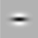
|
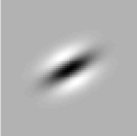 |
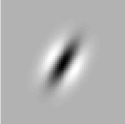 |
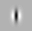 |
 |
 |
|---|---|---|---|---|---|
|
 |
 |
 |
 |
 |

|
 |
 |
 |
 |
 |
From the explicit expression for the Fourier transform, we can in turn obtain the continuous Fourier transform over an infinite discrete spatial domain by letting , which gives
| (40) | ||||
The corresponding discrete Fourier transform over a finite image of size can then be obtained by setting and for and , which gives
| (41) | ||||
Up to numerical errors in an FFT algorithm, we can thereby from these explicit expressions for the Fourier transform of the discrete affine Gaussian kernels generate discrete affine Gaussian kernels and compute convolutions with them with spatial covariance matrices that are exactly equal to the corresponding spatial covariance matrices of the continuous theory. Hence, there is no need for resolving to an approximate numerical method for computing the discrete affine Gaussian scale-space representation. What remains is to determine the free parameter in the spatial discretization as function of the parameters , and that determine the spatial covariance matrix of the discrete affine Gaussian kernel.
Note, however, that although being a much better spatial discretization, in the sense of preserving scale-space properties for the discrete implementation compared to (i) discretizing affine Gaussian receptive fields by spatial sampling, (ii) sampling the Fourier transform of the affine Gaussian kernel or by using (iii) affine warping alternatively (iv) an implementation in terms of recursive filters as outlined in Section 3, the primary type of implementation that we are aiming at for purposes of practical implementation is not only a Fourier-based implementation of discrete affine Gaussian receptive fields. This Fourier-based model is intended for two purposes: (i) as an idealized theoretical model to be used also for practical implementation in situations where an FFT-implementation of the spatial smoothing operation can be regarded as affordable given the external conditions, to make it possible to compute maximally accurate discrete receptive fields, and (ii) a reference and benchmark to be used for comparisons in relation to the additional discretization in the scale direction that will be treated later in Section 6.
5.3 Free parameter and positivity constraint
There is one free parameter in (28), which controls the addition of a discretization of the mixed fourth-order derivative . By combining (23)–(26) with the positivity condition , it follows that a necessary and sufficient condition for obtaining a discretization with non-negative filter coefficients is that the free parameter must satisfy
| (42) |
The feasibility condition arising from this positivity constraint is always more restrictive than the condition for the infinitesimal generator in (29) to be positive semi-definite. This implies that highly eccentric affine Gaussian kernels cannot be represented by non-negative discrete scale-space kernels on a square discrete grid, unless the orientation of the filter is approximately aligned to the coordinate directions.
To analyse for which positive definite covariance matrices the positivity condition may be violated, let us reparameterize the covariance matrix in terms of its eigenvalues as well as the orientation of the eigenvectors
| (43) | ||||
| (44) | ||||
| (45) | ||||
Then, the positivity requirement assumes the form
| (46) |
which can be rewritten as
| (47) |
or equivalently
| (48) |
The “worst case orientation” is given by , and violations of the positivity requirement start to occur when and obey the relation
| (49) |
corresponding to a ratio of the eigenvalues equal to
| (50) |
As long as the eccentricity of the affine Gaussian kernels is lower than this value, we can, however, represent the affine Gaussian scale-space kernels by a non-negative discretization.
This result was stated in Lindeberg [45, Section 3.3] with the derivation left out because of space constraints. A similar bound on the positivity requirement has been derived by Weickert [77] in the context of non-negative discretizations of non-linear diffusion equations. In relation to Weickert’s analysis, the derivation here is shorter.
If we consider the task of representing the distribution of affine Gaussian kernels as parameterized by spatial covariance matrices on the hemisphere as illustrated in Figure 5, then the bound (50) on the eccentricity as obtained from a positivity constraint corresponds to an angle on the hemisphere relative to the north pole of
| (51) |
5.4 Behaviour for low frequencies
By transforming the Fourier transform (LABEL:eq-FT-semi-disc-aff-scsp) of the discrete affine Gaussian kernel to polar coordinates , and performing a Taylor expansion for low angular frequencies
| (52) | ||||
we can with rewrite this expression as
| (53) | ||||
In the specific case when , we can note that the choice implies that
| (54) |
and we obtain a Fourier transform in which the fourth-order terms have a similar angular dependency, here an elliptic shape, as the second-order terms. Indeed, this elliptic shape also coincides with the shape of the corresponding Fourier transform of the Gaussian kernel on a continuous spatial domain.
In the specific case when and , the choice of does in turn correspond to the following discretization of the isotropic diffusion equation (Lindeberg [42, 44])
| (55) |
with and denoting the numerical five-point and the cross-operators, respectively, defined by (Dahlquist et al. [12])
| (56) | ||||
| (57) | ||||
for and corresponding to the following composed computational molecule
| (58) |
which gives the discrete approximation of the Laplacian operator with highest degree of rotational symmetry (Dahlquist et al. [12]).
5.5 Choice of the free parameter
In view of the above analysis, specifically with the condition (42) on necessary relations between the free parameter in relation to the parameters , and of the covariance matrix, we can choose
| (59) |
This is the minimal choice and leads to the discrete kernel with lowest fourth-order moments. (Note that for continuous Gaussian kernels, the fourth-order moments as well as all other moments of order higher than two should be zero.)
5.6 Discrete approximation of scale-space derivatives
Given the above discrete affine Gaussian kernels, we can in turn compute discrete approximations of directional derivatives according to
| (60) | ||||
| (61) | ||||
| (62) | ||||
| (63) | ||||
| (64) | ||||
where , , , and denote discrete approximations to the partial derivative operators , , , and , respectively, and we can preferably choose these of the same types as the discrete approximation operators (20) and (21) used for discretizing the continuous affine diffusion equation (2) into the semi-discrete affine diffusion equation (28) as well as in the generator of its solution (30) and (LABEL:eq-FT-semi-disc-aff-scsp).
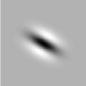
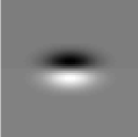
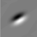
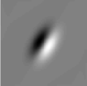
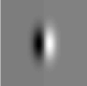
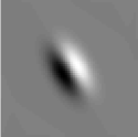
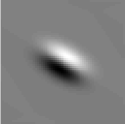
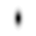
The middle and the top rows in Figure 6 show examples of discrete affine derivative approximation kernels generated in this way from discrete affine Gaussian kernels generated from the explicit expression of the Fourier transform (LABEL:eq-FT-semi-disc-aff-scsp) and with according to (59).
By applying corresponding discrete derivative approximation kernels to the colour-opponent channels and according to a colour-opponent representation (7), we obtain discrete affine Gaussian colour-opponent directional derivative approximations analogous to the colour-opponent receptive fields shown in figure 2.
Note that when we apply these affine Gaussian derivative approximation receptive fields in practice, we do never compute these kernels explicitly. Instead, we apply the compact support discrete directional derivative approximation kernels (60)–(64) directly to the output of the discrete affine Gaussian smoothing as obtained after the FFT implementation of discrete affine Gaussian kernels. In this way, the spatial smoothing operation, which constitutes the computationally most expensive part of a discrete derivative approximation computation, can be shared between directional derivative operations of different spatial orders, thus improving the computational efficiency.
6 Discretization over scale into iteration kernels
In this section, we will show how the theory presented in previous section leads to an implementation scheme based on compact -kernels, when complemented by a discretization in the scale direction.
6.1 Compact -kernel for discrete affine Gaussian smoothing
By further discretizing the semi-discrete affine diffusion equation (28) with respect to the scale parameter using Euler’s forward method (Dahlquist et al. [12])
| (65) |
we obtain the discrete iteration formula
| (66) | ||||
with the following computational molecule for forward iteration by a filter kernel:
| (67) |
This kernel has spatial mean vector
| (68) |
and spatial covariance matrix
| (69) |
Thereby, in analogy with the semi-discrete affine Gaussian scale-space concept over a continuous scale parameter , also the covariance matrices obtained from repeated forward iteration of the kernel by steps will be exactly equal to the covariance matrices of the corresponding continuous affine Gaussian kernels
| (70) |
In Equation (LABEL:eq-disc-Euler-forward-aff-diff-eq), the fully discrete affine scale-space representations will for be numerical approximations
| (71) |
of the exact semi-discrete affine scale-space representation according to (28).
6.2 Choice of scale step
In this section, we will analyse how large scale steps can be taken with the discrete iteration kernel (67) while preserving scale-space properties or transfers thereof.
6.2.1 Normalization of the parameters of the covariance matrix
Since the scale step interacts with the parameters , , , along a cone, we shall specifically choose to normalize the parameters , , and such that the maximum eigenvalue of the covariance matrix according to the parameterization (43), (44) and (45) is given by
| (72) |
and thus the second eigenvalue is
| (73) |
With regard to our goal of discretizing the manifold of affine Gaussian receptive fields over all covariance matrices as illustrated in Figure 5, this parameterization has a very natural geometric interpretation. Assume that the central point in a first image of a scene shows a local surface pattern viewed from a point along the direction of the surface normal at some depth , and that we compute isotropic Gaussian receptive field responses at scale with the parameters of the covariance matrix given by and . Next, assume that we view the same local surface pattern from the same distance while from some other oblique direction with slant angle relative to the surface normal and corresponding to a local foreshortening factor of . Then, the second view should in an affine covariant manner be represented at scale for a covariance matrix with eigenvalues and with the parameter that determines the eigendirections of the covariance matrix directly related to the local tilt direction.
In the following, we will throughout make use of such a parameterization of the covariance matrix for expressing the magnitude of the scale step .
6.2.2 Analysis for the case of the isotropic diffusion equation
To illustrate how the choice of the complementary filter parameter in (27) interrelates with how large scale steps one may take, let us initially consider a discretization of the isotropic diffusion equation for and for the specific choice of in (55) and corresponding to . This leads to a forward iteration kernel of the form
| (74) |
In (Lindeberg [42, 44]) a complete scale-space theory is developed for one-dimensional discrete signals and for isotropic higher-dimensional images over a symmetric spatial domain. In the one-dimensional version of this theory, spatial discretizations of the one-dimensional diffusion equation as obtained from Euler’s forward method lead to kernels of the form
| (75) |
Based on the complete classification of discrete scale-space kernels over a 1-D domain, it is furthermore shown that such discretizations are true discrete scale-space kernels in the one-dimensional sense of guaranteeing non-creation of new local extrema or new zero-crossings from finer to coarser temporal scales if and only if
| (76) |
Specifically, the boundary case corresponds to forward iteration with the binomial kernel
| (77) |
in which the central kernel value is twice as large as its nearest neighbours having values equal to . If we apply a corresponding criterion to the two-dimensional forward iteration kernel (74), we obtain leading to the requirement
| (78) |
If we next again for the isotropic case of and , consider a discretization in the scale direction of (55) for a general value of the parameter , we obtain a forward iteration kernel of the form (Lindeberg [44, Equation (4.39)])
| (79) |
This kernel can be shown to be separable only if (Lindeberg [44, Proposition 4.15]). The corresponding one-dimensional kernel for is then a one-dimensional discrete scale-space kernel only if
| (80) |
where the boundary case corresponds to forward iteration with the kernel
| (81) |
This kernel is a common iteration kernel for computing pyramid representations (Crowley [9]; Crowley and Parker [11, 10]; Lindeberg [42, 44]; Lindeberg and Bretzner [52]). Specifically, applying the underlying one-dimensional kernel for separable convolution twice in the same direction gives a binomial kernel of the form within the family of kernels of length five derived by Burt and Adelson [7] for , which is in very good agreement with the numerical value that they derived empirically.
Note that if we would apply the same value of to the kernel (74) that arises from a spatial discretization of the isotropic diffusion equation for and corresponding to , we would obtain a forward iteration kernel of the form
| (82) |
which would clearly not be a desirable kernel for scale-space filtering. For example, this kernel is not even unimodal. Thus, by the use of a non-zero value of and corresponding to a non-zero value of , in this specific case corresponding to , we can increase the value at the central position of the kernel in relation to its nearest neighbours along the coordinate axes and are thereby be able to take longer steps in the scale direction.
6.2.3 Analysis for the non-isotropic diffusion equation
In this section, we will consider discretizations of the affine Gaussian diffusion equation for general non-zero values of and and also without assuming . Specifically, with a normalization of the parameters of the covariance matrix to the maximum eigenvalue equal to one, we will consider the possibility of taking scale steps up to so that the discrete binomial kernel (81) that represents the maximum possible scale step based on isotropic discrete scale-space theory is regarded as an upper bound on how much spatial smoothing is allowed in different spatial directions.
Requirement on the relations between the kernel values along the coordinate axes and the central point
If we inspired by the ratio of two between the kernel value at the center and the value at the nearest neighbouring points for the kernel (81) that represents the maximum possible smoothing for the isotropic diffusion equation, apply a corresponding criterion that the kernel values at the nearest four-neighbours to the central point having indices should have values that are not greater than half the value of the central point with index , we obtain the conditions
| (83) | ||||
| (84) | ||||
which can be summarized into
| (85) |
If we inspired by the above theoretical analysis for the isotropic case would like to be able to take scale steps up to for general anisotropic discrete affine Gaussian kernels, we obtain the following condition for the values of the nearest four-neighbours to not exceed half the value at the central point
| (86) |
where specifically the case corresponds to .
Requirement on the relations between the kernel values at the corners and the central point
If we apply a condition that the kernel values at the corners having indices should have values that are not greater than one fourth of the value at the central point, we obtain the condition
| (87) |
which can be simplified to to
| (88) |
If we again inspired by the theoretical analysis for the isotropic case would like to take scale steps up to for general anisotropic discrete affine Gaussian kernels, then we obtain the following condition for the values at the corners should not exceed one quarter of the value at the central point
| (89) |
For the specific assumption about the parameters , and corresponding to a covariance matrix with maximum eigenvalue with the other eigenvalue , this condition can according to (43), (44) and (45) be written
| (90) |
The worst case condition arises when , for which the inequality can be reduced to
| (91) |
and which is consistent with the assumptions, thus showing that the condition (89) is guaranteed to hold for all relevant combinations of , and .
6.3 Choice of the free parameter
In view of the above analysis, specifically with the conditions (42) and (86) on necessary relations between the free parameter in relation to the parameters , and of the covariance matrix, we can given the a priori choice of scale step choose
| (92) |
This is the minimal choice and leads to the discrete kernel with lowest fourth-order moment. (Note again that for continuous Gaussian kernels, the fourth-order moment as well as all other moments of order higher than two should be zero.)
The bottom row in figure 7 shows examples of discrete affine kernels generated in this way from repeated application of -kernels of the form (67) for and with according to (92).
Alternatively, one can choose the degrees of freedom within the constraint
| (93) |
to minimize the deviations of the fourth-order terms in the Fourier transform (5.4) from an elliptic behaviour or some other measure of the deviations from affine isotropy. Since such an analysis does, however, become technically more complicated, we will not develop that theory further in this treatment.
6.4 Discrete approximation of scale-space derivatives
When computing discrete approximations to directional derivatives of these discrete affine Gaussian kernels, we can proceed in a similar way as for the discrete affine Gaussian kernels obtained via an FFT and define discrete directional derivative operators , , , and according to equations (60)–(64).
The middle and the top rows in figure 7 show examples of discrete affine derivative approximation kernels generated in this way from repeated iteration of -kernels of the form (67) for , , and with according to (92).
By applying corresponding discrete derivative approximation kernels to the colour-opponent channels and according to a colour-opponent representation (7), we obtain discrete affine Gaussian colour-opponent directional derivative approximations analogous to the colour-opponent receptive fields shown in figure 2.
Note that when we apply these affine Gaussian derivative approximation receptive fields in practice, we do never generate these kernels explicitly. Instead, we apply compact support discrete directional derivative approximation kernels (60)–(64) directly to the output of iterative application of the -kernel (67).
In Section B, we show how this discrete affine scale-space concept can be complemented by spatial subsampling, to generate affine hybrid pyramids, which allow for computationally more efficient smoothing operations at coarser spatial scales, by allowing for both coarser steps in the scale direction and computations over a lower number of image pixels at coarser levels of resolution as depending on the scale level.
7 Scale-normalized derivatives for affine Gaussian scale space
7.1 Continuous affine Gaussian derivative kernels
When defining scale-normalized derivatives for the continuous affine Gaussian derivative based receptive fields of the form , we use the eigenvalues and of the spatial covariance matrix as scale parameters
| (94) |
where and denote possibly different scale normalization powers for the two orthogonal directions and and specifically the choice implies maximal scale invariance.
7.2 Discrete affine Gaussian derivative approximation kernels
For discrete approximations of affine Gaussian derivatives obtained by applying the discrete directional derivative approximations according to (60)–(64) to either the semi-discrete affine scale-space concept according to (28) or the scale-discretized scale-space concept corresponding to repeated application of the -kernel (67), we can in a corresponding manner define variance-normalized affine Gaussian scale-space derivative approximations according to
| (95) |
where denotes the directional derivative approximation operator generalizing the definitions in (60)–(64) and with the implicit understanding that and , etc.
Alternatively, we can define scale-normalized affine Gaussian derivative approximations from -normalization by requiring that the discrete -norm of the discrete derivative approximation kernel being equal to the continuous -norm of the corresponding continuous Gaussian derivative operator
| (96) |
with the affine scale normalization factor determined such that
| (97) |
In the absence of further information, the most scale-invariant choice is to use for .
8 Summary and discussion
The affine Gaussian derivative model constitutes a canonical model for visual receptive fields over a spatial image domain. As we described in Section 2, this model can be derived by necessity from assumptions that reflect structural properties of the world in combination with requirements to ensure internal consistency between image representations at different scales. The receptive field profiles predicted by this theory do furthermore well model the spatial shapes of the receptive fields of simple cells in the primary visual cortex (V1). Thus, this model can be motivated both mathematically/physically and from a biological viewpoint. The close similarity between the results obtained from mathematical/physical arguments vs. the properties of biological receptive fields, as resulting from ages of evolutionary pressure, strongly support that this should be an appropriate computational model for spatial visual receptive fields.
Compared to the more commonly used Gaussian derivative model based on spatial derivatives of the rotationally symmetric Gaussian kernel, the family of affine Gaussian derivative kernels based on directional derivatives of affine Gaussian kernels is additionally covariant under local affine transformations of the spatial domain. This property allows for more accurate modelling of receptive field measurements under perspective transformations, which in turn enables the development of more robust computer vision algorithms under the geometric transformations that arise when observing a 3-D world using a 2-D image sensor.
From these properties together, it is natural to propose a design strategy for a vision system, where affine Gaussian derivative kernels are used as a first layer of visual receptive fields applied to the raw input images, and then higher-layer visual operations use the output from these affine Gaussian derivatives as input. The theory for affine Gaussian derivatives is, however, fully continuous, assuming image functions defined over a continuous spatial domain. This raises the question about how to discretize this theory for a discrete implementation, while still preserving as many as possible of the desirable properties that define the uniqueness of the affine Gaussian derivative kernels in the continuous case.
To address this problem, we have presented a theory for discretizing the affine Gaussian scale-space concept underlying the affine Gaussian derivative model, so that scale-space properties hold also in a discrete sense for the discrete implementation. Specifically, we have presented two types of spatial discretizations of the continuous affine diffusion equation that describes the effect of convolution with affine Gaussian kernels: (i) a semi-discretization over space only while leaving the continuous scale parameter in terms of a family of spatial covariance matrices defined over a continuum and (ii) an additional discretization in the scale direction that leads to compact kernels to be applied repeatedly, to compute discrete affine Gaussian scale-space representations at successively coarser scales, for families of discrete affine Gaussian kernels of different size, orientation and eccentricity.
The first theory is defined uniquely from similar assumptions as constitute the scale-space axioms that define the uniqueness of the affine Gaussian kernel over a continuous spatial domain. A fully axiomatic derivation of this model is given in Appendix A. For the second theory, the restriction to local kernels of size is implied by necessity from the locality property implied by the assumption of non-enhancement of local extrema, which constitutes our formalization of the requirement that new structures must not be created from finer to coarser scales.
A third option is to combine the smoothing process in the second model with spatial subsampling operations at coarser spatial scales, leading to the notion affine hybrid pyramids for improving both the computational efficiency and the memory requirements at coarser spatial scales.
These three families of discrete affine Gaussian kernels can in turn be combined with discretizations of spatial directional derivative operators for computing discrete approximations of directional derivatives, leading to families of discrete affine Gaussian derivative approximations, which are intended to serve as a basis for expressing later stage visual processes.
For these three types of spatial discretization approaches, we have additionally solved a number of technical problems:
- •
-
•
For the first semi-discrete model, we have analysed the influence of a remaining free parameter in the theory, not determined by the primary assumptions (Sections 5.3–5.5). We have stated necessary and sufficient conditions to ensure a positive discretization (Equation (42)) and shown how this parameter in specific cases can be optimized for achieving better numerical approximation of rotational symmetry or affine angular dependency of the Fourier transform (Section 5.4) or minimizing the fourth-order moments of the discrete smoothing kernel (Section 5.5).
-
•
For the second fully discrete model, while without spatial subsampling, we have derived an explicit parameterization of compact -kernels in terms of the contribution they give to the spatial covariance of the composed discrete affine Gaussian kernel (Equation (67)) and analysed how the scale step in the scale direction can be determined when applying these -kernels repeatedly (Section 6.2). We have also analyzed how the free parameter can be determined within the positivity constraints (Section 6.3) and proposed the specific choice (92) for choosing this parameter as function of the elements , and in the affine covariance matrix .
-
•
For the third fully discrete model, also involving spatial subsampling at coarser spatial scales, we have proposed an algebra for defining reduction operators from finer to coarser spatial scales (Section B.1) as well as a criterion for measuring how much spatial smoothing needs to be applied (depending on the eccentricity of the anisotropic spatial smoothing kernels) before the affine hybrid pyramid representation may be spatially subsampled (Equation (128)). We have specifically proposed ways of measuring the scale levels and the subsampling rate in the presence of spatial subsampling and shown how equivalent discrete derivative computation kernels can be defined to in turn allow for the definition of appropriate scale normalization factors (138) in the presence of spatial subsampling (Sections B.3–B.5).
Out of the three presented spatial discretization models, the first semi-discrete model allows for the most accurate discrete implementation, in the sense of mimicking the corresponding continuous scale-space properties. This model can be implemented with reasonable efficiency using a closed-form expression for the discrete Fourier transform of the discrete affine Gaussian kernel (LABEL:eq-FT-semi-disc-aff-scsp). If an inverse Fourier transform for each layer in the affine scale-space representation is regarded as requiring too much computational work, a discrete implementation based on repeated application of the -kernels (67) according to the second discretization model may be computationally more efficient, at least at finer scale levels, specifically on massively parallel architectures such as GPUs. From such a conceptual background, the semi-discrete Fourier-based implementation can be regarded as a reference, to optimize the implementation based on repeated application of -kernels against. If an implementation based on repeated application of -kernels using the same resolution at all scale levels is still regarded as requiring too much computational work with respect to the task at hand, then an affine hybrid pyramid implementation should be chosen, with the minimum amount of necessary smoothing before a subsampling stage as determined by the spatial smoothing parameter in (128) and leading to the subsampling rate according to (140) optimized to lead to an appropriate trade-off between numerical accuracy and computational efficiency. If on the other hand, coarser scale representations are to be computed frequently, and if a Fourier-based implementation is affordable, then the first semi-discrete Fourier-based method can be chosen, since it is the most accurate of these three methods. Thus, the presented theory offers three main alternatives, depending on the complexity and the accuracy requirements of the visual task vs. the available computational resources.
A limitation of the presented genuinely discrete affine Gaussian scale-space concepts, however, is that the requirement of a positive discretization, as implied by the discrete scale-space axioms underlying the formulation of the theory, implies a bound on the ratio between the maximum and minimum eigenvalues of the spatial covariance matrix that determines the shapes of the affine Gaussian kernels. The theoretical analysis in Section 5.3 gives an upper bound on the eccentricity corresponding to the amount of foreshortening caused by a slant angle of . While not covering extreme amounts of foreshortening, this bound still enables handling of basic use cases for expressing affine covariant image operations between multiple views of the same object. If higher amounts of foreshortening are to be handled, alternatives beyond the ad hoc solution of just imposing an upper bound on the eccentricity according to the stated criterion, are to investigate numerical approximations of the continuous model using alternative discretizations as outlined in Section 3.
We propose that the presented theory can be used for generating different architectures for early visual operations based on affine Gaussian derivative kernels or extensions thereof. The most straightforward type of architecture consists of extending the use of a regular Gaussian scale-space representation, based on rotationally symmetric Gaussian kernels over multiple spatial scales, to an affine Gaussian scale-space representation over both spatial scale levels, orientations in image space and eccentricities in terms of ratios between the scale values in the two orthogonal eigen-directions of the affine Gaussian kernel. Thus, in a first step a set of covariance matrices representing affine Gaussian kernels of different orientations and different eccentricities may be generated analogous to the sample tesselation on a hemisphere as shown in Figure 5 or a rectangular tesselation over the sizes, orientations and eccentricities of the affine Gaussian kernels. Then, for each orientation and each eccentricity, a set of affine Gaussian scale-space representations with associated affine Gaussian derivatives can be computed for a set of scale values, according to either of the three presented discretization models. This representation can in turn be used as input for a vision system addressing one or several visual tasks under substantial image deformations caused by significant perspective effects.
Appendix A Non-isotropic scale-space for discrete signals: Necessity and sufficiency
This appendix presents a general theoretical result concerning linear shift-invariant scale-space representations of discrete signals over an anisotropic -dimensional domain. The result is a generalization of earlier results presented in (Lindeberg [42, 44]) for isotropic discrete scale spaces.
A.1 Definitions
Let us state this (minimal) set of basic properties a family should satisfy to be a candidate family for generating a linear scale-space.
Definition A.1.
(Discrete pre-scale-space family of kernels)
A one-parameter family of kernels
is said to be a discrete pre-scale-space family of kernels
if it satisfies
-
•
,
-
•
the semi-group property ,
-
•
the continuity requirement when .
Definition A.2.
(Discrete pre-scale-space representation) Let be a discrete signal and let be a discrete pre-scale-space family of kernels. Then, the one-parameter family of signals given by
| (98) |
is said to be the discrete pre-scale-space representation of generated by .
Lemma A.3.
(A discrete pre-scale-space representation is differentiable)
Let be the
discrete pre-scale-space representation of a signal
in .
Then, satisfies the differential equation
| (99) |
for some linear and shift-invariant operator .
Proof: If is sufficiently regular, e.g., if , define a family of operators , here from from to , by . Due to the conditions imposed on the kernels, the family satisfies the relation
| (100) |
where is the identity operator. Such a family is called a strongly continuous semigroup of operators (Hille and Phillips [28, pages 58–59]) A semi-group is often characterized by its infinitesimal generator defined by
| (101) |
The set of elements for which exists is denoted . This set is not empty and never reduces to the zero element. Actually, it is even dense in (Hille and Phillips [28, page 307]). If this operator exists then
| (102) |
According to a theorem in Hille and Phillips [28, page 308], strong continuity implies for all . Hence, the scale-space family must obey the differential equation for some linear operator . Since is generated from by a convolution operation, it follows that must be shift-invariant.
Definition A.4.
(Pre-scale-space property: Non-enhancement of local extrema)
A discrete pre-scale-space representation
of a discrete signal
is said to possess
pre-scale-space properties, or equivalently not to enhance
local extrema,
if for every value of the scale parameter it holds that
if is a local maximum or a local minimum for the
mapping , then the derivative
of with respect to satisfies
| (103) | ||||
| (104) | ||||
Definition A.5.
(Discrete scale-space family of kernels) A one-parameter family of discrete pre-scale-space kernels is said to be a discrete scale-space family of kernels if for any discrete signal the discrete pre-scale-space representation of generated by possesses pre-scale-space properties, i.e., if for any signal local extrema are never enhanced.
Definition A.6.
(Discrete scale-space representation) A discrete pre-scale-space representation of a signal generated by a family of discrete kernels , which are discrete scale-space kernels, is said to be a discrete scale-space representation of .
A.2 Necessity
Theorem A.7.
(Scale-space for discrete signals: Necessity)
A discrete scale-space representation
of a
discrete signal satisfies the
differential equation
| (105) |
with initial condition for some infinitesimal scale-space generator characterized by:
-
•
the locality condition if ,
-
•
the positivity constraint if and
-
•
the zero sum condition .
Proof: The proof consists of two parts. The first part has already been presented in Lemma A.3, where it was shown that the requirements on the kernels imply that the family obeys a linear differential equation. Because of the shift invariance, can be written on the form
| (106) |
In the second part, counterexamples will be constructed from various simple test functions in order to delimit the class of possible operators.
Step 1
Let denote the set of points around within distance 1 in maximum norm, i.e., . Let furthermore denote the corresponding neighbourhood of , by excluding the central point.
The extremum point conditions (103) and (104) combined with Definitions A.5–A.6 mean that must be local, i.e., that if . This can be easily understood by studying the following counterexample: First, assume that for some and define a function by
| (107) |
Obviously, is a local maximum point for . From (13) one obtains . It is clear that this value can be positive provided that is chosen small enough. Hence, cannot satisfy (103). Similarly, it can also be shown that leads to a violation of the non-enhancement property (104) (let ). Consequently, must be zero if .
Step 2
With the assumed weak definitions of local extremum points, it is clear that for a constant input function , the point is both a local maximum point and a local minimum point. Hence must be zero, which implies that the coefficients must sum to zero
| (108) |
Step 3
Finally, by observing that due to the zero sum condition, (13) can be written
| (109) |
By considering the test function
| (110) |
for some in , one easily realizes that must be non-negative if .
The initial condition is a direct consequence of the definition of the notion of a pre-scale-space kernel.
A.3 Sufficiency
Theorem A.8.
(Scale-space for discrete signals: Sufficiency)
Given an infinitesimal generator corresponding to
| (111) |
where the coefficients satisfy
-
•
the locality condition if ,
-
•
the positivity constraint if and
-
•
the zero sum condition ,
the solution of the diffusion equation
| (112) |
with initial condition constitutes a discrete scale-space representation. Specifically, obeys
| (113) | ||||
| (114) | ||||
Proof: From (109) it follows that the influence of at any extremum point in scale-space can be written
| (115) |
If is a local maximum, then all differences are negative. Combined with the positivity of , it follows that . If is a local minimum, we apply the same way of reasoning to .
Appendix B Affine hybrid pyramids
In this section, we will show how the fully discretized affine Gaussian scale-space concept presented in Section 6 in the main article can be combined with spatial subsampling, to allow for computationally more efficient smoothing operations at coarser spatial scales. The motivation for this approach is similar to the motivations underlying regular spatial pyramids: At coarser scales, when the image representations become gradually smoother, the image values to also become gradually more redundant, implying that the loss of accuracy caused by spatial subsampling will be lower.
Specifically, we will show how repeated filtering with our derived kernel according to (67) can be combined with spatial subsampling operations to compute the discrete affine Gaussian scale-space representations at coarser scales in a computationally more efficient manner compared to using the same resolution at all levels of scale. Consider the upper bound on the scale step as holds for the isotropic diffusion equation (Equation (80)) and which can also be extended to the non-isotropic diffusion equation (Section 6.2.3). By applying this upper bound relative to the current resolution after spatial subsampling stages by a factor of 2, the effective bound on the spatial step will become
| (116) |
thus implying that larger scale steps can be taken and at fewer iterations will thus be needed to reach the coarser scale representations. In addition, the computations will be done on a substantially lower number of pixels, with the number of pixels divided by a factor of . Together, this implies that the computational efficiency will be improved by two main factors that both increase exponentially with the amount of spatial subsampling. This will lead to an extension of isotropic pyramid and hybrid pyramid representations (Burt and Adelson [7]; Crowley [9]; Crowley and Parker [11, 10]; Lindeberg and Bretzner [52]) to the notion affine hybrid pyramid representations.
B.1 Reduction operators
Following Burt and Adelson [7]; Crowley [9]; Crowley and Parker [11, 10] and Lindeberg and Bretzner [52]), let us describe the transformation between two adjacent resolution levels in a pyramid by a reduction operator. For simplicity, let us assume that the size of the smoothing filter is the same over both the coordinate directions and odd. Then, the transformation from the representation at the current resolution level , to the representation at the next coarser resolution level is for some set of filter coefficients given by
| (117) | ||||
| (118) | ||||
where is the spatial subsampling factor. Next, let us assume that the smoothing operation can be decomposed into several smoothing steps:
| (119) |
|
where the notation means that several operators of the form may occur. is thus composed of one or more smoothing operations followed by a subsampling step. The subsampling operation is here defined by
| (120) | ||||
| (121) | ||||
where again we usually choose and where each smoothing step is of the form
| (122) | ||||
| (123) | ||||
Specifically, we assume that the coefficients of the smoothing operation originate from the -kernel (67) arising from the discretization of the diffusion operator
| (124) |
which in turn will be repeated times at each level of resolution, corresponding to an affine hybrid pyramid with the following structure over spatial scales as reflecting variations in the size in the image domain
| (125) |
|
and with such a representation computed for each orientation and eccentricity to reflect a grid-based sampling over the three-parameter family of affine Gaussian kernels. The grid spacing as function of the resolution level will be given by
| (126) |
if we adopt the convention that should correspond to the original resolution.
B.2 Eccentricity-dependent spatial subsampling
A particular factor that needs to be taken into account when computing a hybrid pyramid representation based on affine smoothing kernels is that amount of smoothing will be different in different spatial directions. Let us adopt the convention from hybrid pyramids computed from spatially isotropic binomial kernels (Lindeberg and Bretzner [52]), where a binomial- pyramid can be constructed by applying spatial smoothing steps with scale step before a spatial subsampling stage is permitted. Then, the total amount of smoothing before the subsampling operation is at any level of resolution equal to
| (127) |
in units of a normalized grid spacing with . Let us next for an affine hybrid pyramid representation assume that the spatial covariance matrix is normalized such that the maximum eigenvalue . Then, the minimum amount of spatial smoothing over all directions in image space is given by .
To compute an affine hybrid pyramid with the same guaranteed minimum amount of spatial smoothing as for a regular binomial- pyramid based on spatially isotropic smoothing kernels with and , we then have to stay at the same level of spatial resolution as long as the iteration index within any level of resolution satisfies
| (128) |
Thus, the spatial subsampling operation has be applied more restrictively for highly eccentric/anisotropic spatial smoothing kernels compared to more isotropic kernels.
Equivalent affine hybrid pyramid kernels for
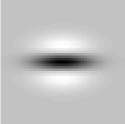
|
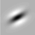 |
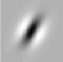 |
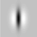 |
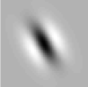 |
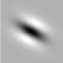 |
|---|---|---|---|---|---|
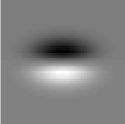
|
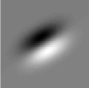 |
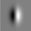 |
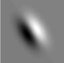 |
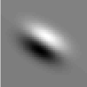 |
|
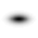
|
 |
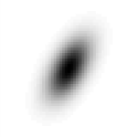 |
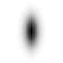 |
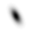 |
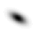 |
Equivalent spatio-chromatic affine hybrid pyramid kernels for
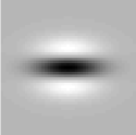
|
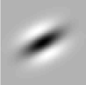 |
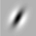 |
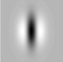 |
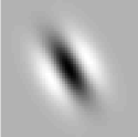 |
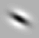 |
|---|---|---|---|---|---|
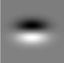
|
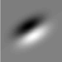 |
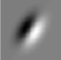 |
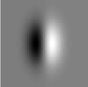 |
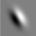 |
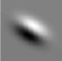 |

|
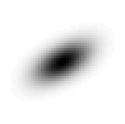 |
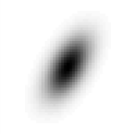 |
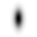 |
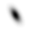 |
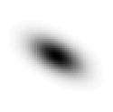 |
Equivalent spatio-chromatic affine hybrid pyramid kernels for

|
 |
 |
 |
 |
 |
|---|---|---|---|---|---|
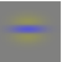
|
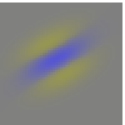 |
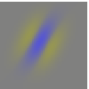 |
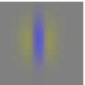 |
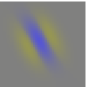 |
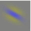 |
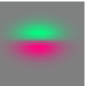
|
 |
 |
 |
 |
 |
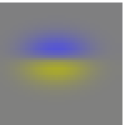
|
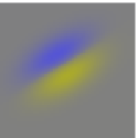 |
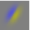 |
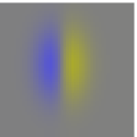 |
 |
 |
Equivalent spatio-chromatic affine hybrid pyramid kernels for

|
 |
 |
 |
 |
 |
|---|---|---|---|---|---|
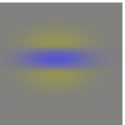
|
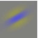 |
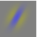 |
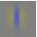 |
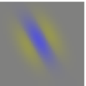 |
 |
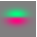
|
 |
 |
 |
 |
 |
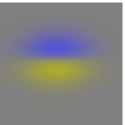
|
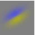 |
 |
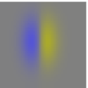 |
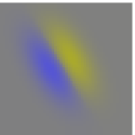 |
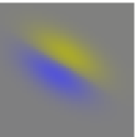 |
A higher value of will, in general, lead to equivalent discrete derivative approximation kernels that constitute numerically better approximations in relation to the discrete affine Gaussian kernels expressed over a constant grid spacing (see Figures 9–9), whereas a lower value of will lead to higher computational efficiency. To guarantee a sufficient minimum amount of spatial smoothing before the spatial subsampling operation is performed, we recommend that should be chosen at least greater than two:
| (129) |
In relation to an isotropic regular pyramid representation for and , the lower bound on the minimum amount of spatial smoothing required in this way corresponds to the amount of spatial smoothing obtained by applying separable smoothing with the binomial kernel along each dimension, which constitutes a common way of generating classic image pyramids (Crowley [9]; Burt and Adelson [7]; Crowley and Parker [11, 10]; Lindeberg [42, 44]; Lindeberg and Bretzner [52]). Since such pyramids may, however, imply undersampling of the image data, we propose a condition of the form instead of , with the complementary recommendation that higher values of will improve the performance of image analysis/computer vision algorithms further.
B.3 Equivalent convolution kernels and derivative approximation kernels
Since the representation at each level is constructed from a set of repeated smoothing and subsampling operations, which are all linear operations, the composed operation can equivalently be modeled as the result of applying one kernel , termed equivalent convolution kernel, to the original image, followed by a pure subsampling step with composed subsampling factor . If we define a dual operator to the operator according to
where the operation enlarges any -dimensional image by a factor
| (130) | ||||
| (131) | ||||
then the equivalent convolution kernel corresponding to resolution level and internal iteration level within this level of resolution can be written
| (132) |
where is a discrete delta function at level and denotes the operators corresponding to the set of all the operators used for reaching this level in the affine hybrid pyramid.
Similarly, derivative approximations can be computed by taking the grid spacing at the current into explicit account
| (133) |
at any level with resolution in the pyramid. Then, the corresponding equivalent derivative approximation kernel will be given by
| (134) |
where higher-dimensional difference approximations are expressed in terms of the one-dimensional th order difference operator
| (135) |
Figures 9–9 show examples of equivalent convolution kernels and equivalent derivative approximation kernels over the grey-level channel for the cases of and . Figures 11–11 show corresponding equivalent derivative approximation kernels over the red/green and yellow/blue colour-opponent channels.
B.4 Scale-normalized derivative approximations
To compute scale-normalized derivatives in an affine hybrid pyramid representation at iteration level within resolution level , we can in a corresponding manner as in Section 7 define variance-normalized directional derivative approximations according to
| (136) |
where denotes the directional derivative approximation operator generalizing the definitions in (60)–(64) with the implicit understanding that and , etc. As spatial scale normalization parameters and , we should take the eigenvalues of the spatial covariance matrix of the equivalent convolution kernel according to (132). With the proposed way of defining affine hybrid pyramids according to (125), the spatial covariance matrix of the equivalent derivative approximation kernel will for every resolution level and iteration level be equal to the spatial covariance matrix predicted by the discretization theory, if we multiply the increments in , as as obtained from the iteration kernel (67) with overall scale step as used as the primitive smoothing kernel in the reduction cycle (125) by with according to (126).
The definition of scale-normalized affine Gaussian derivative approximations from -normalization is analogous to the corresponding case without spatial subsampling (96)
| (137) |
with the only difference that the expression in (97) that defines the scale-normalization factor as function of the spatial scale parameters should be replaced by
| (138) |
with the equivalent discrete derivative approximation operator defined by expanding the discrete directional derivative approximation operator at the corresponding level of resolution according to (134)
| (139) |
and with denoting the grid spacing at the current level of resolution.
B.5 Measuring the subsampling rate
To describe how the grid spacing depends on the scale parameter in a hybrid pyramid, we can introduce a subsampling factor from the relation
| (140) |
assuming that the overall scale parameter represents the total amount of smoothing with the effects of varying grid spacing taken into account, so that the contribution to at any resolution level is given by
| (141) |
and with the eigenvalues and normalized such that and .
For reasons of computational efficiency, we define the actual grid spacing as the maximum power of two that does not exceed this upper bound
| (142) |
Thus, a subsampling factor of corresponds to preserving the original resolution at all levels of scales, whereas increasing values of correspond to higher degrees of subsampling at coarser levels of scale.
References
- [1] Almansa, A., Lindeberg, T.: Fingerprint enhancement by shape adaptation of scale-space operators with automatic scale-selection. IEEE Transactions on Image Processing 9(12), 2027–2042 (2000)
- [2] Ballester, C., Gonzalez, M.: Affine invariant texture segmentation and shape from texture by variational methods. Journal of Mathematical Imaging and Vision 9, 141–171 (1998)
- [3] Baumberg, A.: Reliable feature matching across widely separated views. In: Proc. Computer Vision and Pattern Recognition (CVPR’00), pp. I:1774–1781. Hilton Head, SC (2000)
- [4] Bay, H., Ess, A., Tuytelaars, T., van Gool, L.: Speeded up robust features (SURF). Computer Vision and Image Understanding 110(3), 346–359 (2008)
- [5] Bouma, H., Vilanova, A., Bescós, J.O., ter Haar Romeny, B., Gerritsen, F.A.: Fast and accurate Gaussian derivatives based on B-splines. In: International Conference on Scale Space and Variational Methods in Computer Vision (SSVM 2007), pp. 406–417 (2007). Springer LNCS volume 4485
- [6] Burghouts, G.J., Geusebroek, J.M.: Performance evaluation of local colour invariants. Computer Vision and Image Understanding 113(1), 48–62 (2009)
- [7] Burt, P.J., Adelson, E.H.: The Laplacian pyramid as a compact image code. IEEE Trans. Communications 9:4, 532–540 (1983)
- [8] Conway, B.R., Livingstone, M.S.: Spatial and temporal properties of cone signals in alert macaque primary visual cortex. Journal of Neuroscience 26(42), 10,826–10,846 (2006)
- [9] Crowley, J.L.: A representation for visual information. Ph.D. thesis, Carnegie-Mellon University, Robotics Institute, Pittsburgh, Pennsylvania (1981)
- [10] Crowley, J.L., Parker, A.C.: A representation for shape based on peaks and ridges in the Difference of Low-Pass Transform. IEEE Trans. Pattern Analysis and Machine Intell. 6(2), 156–170 (1984)
- [11] Crowley, J.L., Stern, R.M.: Fast computation of the Difference of Low Pass Transform. IEEE Trans. Pattern Analysis and Machine Intell. 6, 212–222 (1984)
- [12] Dahlquist, G., Björk, Å., Anderson, N.: Numerical Methods. Prentice-Hall (1974)
- [13] Dalal, N., Triggs, B.: Histograms of oriented gradients for human detection. In: Proc. Computer Vision and Pattern Recognition (CVPR 2005), vol. 1, pp. 886–893 (2005)
- [14] DeAngelis, G.C., Anzai, A.: A modern view of the classical receptive field: Linear and non-linear spatio-temporal processing by V1 neurons. In: L.M. Chalupa, J.S. Werner (eds.) The Visual Neurosciences, vol. 1, pp. 704–719. MIT Press (2004)
- [15] DeAngelis, G.C., Ohzawa, I., Freeman, R.D.: Receptive field dynamics in the central visual pathways. Trends in Neuroscience 18(10), 451–457 (1995)
- [16] Deriche, R.: Using Canny’s criteria to derive a recursively implemented optimal edge detector. International Journal of Computer Vision 1, 167–187 (1987)
- [17] Dollár, P., Appel, R., Belongie, S., Perona, P.: Fast feature pyramids for object detection. IEEE Transactions on Pattern Analysis and Machine Intelligence 36(8), 1532–1545 (2014)
- [18] Farid, H., Simoncelli, E.P.: Differentiation of discrete multidimensional signals. IEEE Transactions on Image Processing 13(4), 496–508 (2004)
- [19] Fedorov, V., Arias, P., Facciolo, G., Ballester, C.: Affine invariant self-similarity for exemplar-based inpainting. In: International Conference on Computer Vision and Applications (VISAPP 2016) (2016)
- [20] Fedorov, V., Arias, P., Sadek, R., Facciolo, G., Ballester, C.: Linear multiscale analysis of similarities between images on Riemannian manifolds: Practical formula and affine covariant metrics. SIAM Journal on Imaging Sciences 8(3), 2021–2069 (2015)
- [21] Florack, L.: A spatio-frequency trade-off scale for scale-space filtering. IEEE Transactions on Pattern Analysis and Machine Intelligence 22(9), 1050–1055 (2000)
- [22] Florack, L.M.J.: Image Structure. Series in Mathematical Imaging and Vision. Springer (1997)
- [23] Geusebroek, J.M., Smeulders, A.W.M., van de Weijer, J.: Fast anisotropic Gauss filtering. IEEE Transactions on Image Processing 12(8), 938–943 (2003)
- [24] Giannarou, S., Visentini-Scarzanella, M., Yang, G.G.: Probabilistic tracking of affine-invariant anisotropic regions. IEEE Transactions on Pattern Analysis and Machine Intelligence 35(1), 130–143 (2013)
- [25] ter Haar Romeny, B. (ed.): Geometry-Driven Diffusion in Computer Vision. Series in Mathematical Imaging and Vision. Springer (1994)
- [26] Hall, D., de Verdiere, V., Crowley, J.: Object recognition using coloured receptive fields. In: Proc. European Conf. on Computer Vision (ECCV 2000), Springer LNCS, vol. 1842, pp. I:164–177. Springer, Dublin, Ireland (2000)
- [27] He, K., Zhang, X., Ren, S., Sun, J.: Deep residual learning for image recognition. In: Proc. Computer Vision and Pattern Recognition (CVPR 2016), pp. 770–778 (2016)
- [28] Hille, E., Phillips, R.S.: Functional Analysis and Semi-Groups, vol. XXXI. American Mathematical Society Colloquium Publications (1957)
- [29] Hubel, D.H., Wiesel, T.N.: Receptive fields of single neurones in the cat’s striate cortex. J Physiol 147, 226–238 (1959)
- [30] Hubel, D.H., Wiesel, T.N.: Brain and Visual Perception: The Story of a 25-Year Collaboration. Oxford University Press (2005)
- [31] Iijima, T.: Observation theory of two-dimensional visual patterns. Tech. rep., Papers of Technical Group on Automata and Automatic Control, IECE, Japan (1962). (in Japanese)
- [32] Johnson, E.N., Hawken, M.J., Shapley, R.: The orientation selectivity of color-responsive neurons in Macaque V1. The Journal of Neuroscience 28(32), 8096–8106 (2008)
- [33] Koenderink, J.J.: The structure of images. Biological Cybernetics 50, 363–370 (1984)
- [34] Koenderink, J.J., van Doorn, A.J.: Representation of local geometry in the visual system. Biological Cybernetics 55, 367–375 (1987)
- [35] Koenderink, J.J., van Doorn, A.J.: Generic neighborhood operators. IEEE Trans. Pattern Analysis and Machine Intell. 14(6), 597–605 (1992)
- [36] Krizhevsky, A., Sutskever, I., Hinton, G.E.: ImageNet classification with deep convolutional neural networks. In: Advances in Neural Information Processing Systems, pp. 1097–1105 (2012)
- [37] Larsen, A.B.L., Darkner, S., Dahl, A.L., Pedersen, K.S.: Jet-based local image descriptors. In: Proc. European Conference on Computer Vision (ECCV 2012), Springer LNCS, vol. 7574, pp. III:638–650. Springer (2012)
- [38] Lazebnik, S., Schmid, C., Ponce, J.: A sparse texture representation using local affine regions. IEEE Trans. Pattern Analysis and Machine Intell. 27(8), 1265–1278 (2005)
- [39] Liao, K., Liu, G., Hui, Y.: An improvement to the SIFT descriptor for image representation and matching. Pattern Recognition Letters 34(11), 1211–1220 (2013)
- [40] Lim, J.Y., Stiehl, H.S.: A generalized discrete scale-space formulation for 2-D and 3-D signals. In: International Conference on Scale-Space Theories in Computer Vision (Scale-Space’03), pp. 132–147 (2003). Springer LNCS volume 2695
- [41] Linde, O., Lindeberg, T.: Composed complex-cue histograms: An investigation of the information content in receptive field based image descriptors for object recognition. Computer Vision and Image Understanding 116, 538–560 (2012)
- [42] Lindeberg, T.: Scale-space for discrete signals. IEEE Trans. Pattern Analysis and Machine Intell. 12(3), 234–254 (1990)
- [43] Lindeberg, T.: Discrete derivative approximations with scale-space properties: A basis for low-level feature extraction. Journal of Mathematical Imaging and Vision 3(4), 349–376 (1993)
- [44] Lindeberg, T.: Scale-Space Theory in Computer Vision. Springer (1993)
- [45] Lindeberg, T.: Linear spatio-temporal scale-space. In: Proc. International Conference on Scale-Space Theory in Computer Vision (Scale-Space’97), Springer LNCS, vol. 1252, pp. 113–127. Springer (1997)
- [46] Lindeberg, T.: Linear spatio-temporal scale-space. Tech. Rep. ISRN KTH/NA/P–01/22–SE, Dept. of Numerical Analysis and Computer Science, KTH (2001). Available from http://www.csc.kth.se/cvap/abstracts/cvap257.html
- [47] Lindeberg, T.: Scale-space. In: B. Wah (ed.) Encyclopedia of Computer Science and Engineering, pp. 2495–2504. John Wiley and Sons, Hoboken, New Jersey (2008)
- [48] Lindeberg, T.: Generalized Gaussian scale-space axiomatics comprising linear scale-space, affine scale-space and spatio-temporal scale-space. Journal of Mathematical Imaging and Vision 40(1), 36–81 (2011)
- [49] Lindeberg, T.: A computational theory of visual receptive fields. Biological Cybernetics 107(6), 589–635 (2013)
- [50] Lindeberg, T.: Invariance of visual operations at the level of receptive fields. PLOS ONE 8(7), e66,990 (2013)
- [51] Lindeberg, T.: Time-causal and time-recursive spatio-temporal receptive fields. Journal of Mathematical Imaging and Vision 55(1), 50–88 (2016)
- [52] Lindeberg, T., Bretzner, L.: Real-time scale selection in hybrid multi-scale representations. In: L. Griffin, M. Lillholm (eds.) Proc. Scale-Space Methods in Computer Vision (Scale-Space’03), Springer LNCS, vol. 2695, pp. 148–163. Springer, Isle of Skye, Scotland (2003)
- [53] Lindeberg, T., Gårding, J.: Shape-adapted smoothing in estimation of 3-D depth cues from affine distortions of local 2-D structure. In: J.O. Eklundh (ed.) Proc. European Conf. on Computer Vision (ECCV’94), Lecture Notes in Computer Science, vol. 800, pp. 389–400. Springer-Verlag, Stockholm, Sweden (1994)
- [54] Lindeberg, T., Gårding, J.: Shape-adapted smoothing in estimation of 3-D depth cues from affine distortions of local 2-D structure. Image and Vision Computing 15, 415–434 (1997)
- [55] Lowe, D.G.: Distinctive image features from scale-invariant keypoints. International Journal of Computer Vision 60(2), 91–110 (2004)
- [56] Mikolajczyk, K., Schmid, C.: Scale and affine invariant interest point detectors. International Journal of Computer Vision 60(1), 63–86 (2004)
- [57] Mikolajczyk, K., Tuytelaars, T., Schmid, C., Zisserman, A., Matas, J., Schaffalitzky, F., Kadir, T., van Gool, L.: A comparison of affine region detectors. International Journal of Computer Vision 65(1–2), 43–72 (2005)
- [58] Morel, J.M., Yu, G.: ASIFT: A new framework for fully affine invariant image comparison. SIAM Journal on Imaging Sciences 2(2), 438–469 (2009)
- [59] Rothganger, F., Lazebnik, S., Schmid, C., Ponce, J.: 3D object modeling and recognition using local affine-invariant image descriptors and multi-view spatial constraints. International Journal of Computer Vision 66(3), 231–259 (2006)
- [60] Rothganger, F., Lazebnik, S., Schmid, C., Ponce, J.: Segmenting, modeling, and matching video clips containing multiple moving objects. IEEE Transactions on Pattern Analysis and Machine Intelligence 29(3), 477–491 (2007)
- [61] Sadek, R., Constantinopoulos, C., Meinhardt, E., C. Ballester, C., Caselles, V.: On affine invariant descriptors related to SIFT. SIAM Journal on Imaging Sciences 5(2), 652–687 (2012)
- [62] van de Sande, K.E.A., Gevers, T., Snoek, C.G.M.: Evaluating color descriptors for object and scene recognition. IEEE Trans. Pattern Analysis and Machine Intell. 32(9), 1582–1596 (2010)
- [63] Schaffalitzky, F., Zisserman, A.: Viewpoint invariant texture matching and wide baseline stereo. In: Proc. International Conference on Computer Vision (ICCV 2001), pp. II:636–643. Vancouver, Canada (2001)
- [64] Schiele, B., Crowley, J.: Recognition without correspondence using multidimensional receptive field histograms. International Journal of Computer Vision 36(1), 31–50 (2000)
- [65] Serre, T., Wolf, L., Bileschi, S., Riesenhuber, M., Poggio, T.: Robust object recognition with cortex-like mechanisms. IEEE Transactions on Pattern Analysis and Machine Intelligence 29(3), 411–426 (2007)
- [66] Shapley, R., Hawken, M.J.: Color in the cortex: single-and double-opponent cells. Vision research 51(7), 701–717 (2011)
- [67] Simonyan, K., Zisserman, A.: Very deep convolutional networks for large-scale image recognition. In: International Conference on Learning Representations (ICLR 2015) (2015). ArXiv preprint arXiv:1409.1556
- [68] Sivic, J., Zisserman, A.: Video Google: A text retrieval approach to object matching in videos. In: Proc. International Conference on Computer Vision (ICCV’03), p. 1470 (2003)
- [69] Slavík, A., Stehlík, P.: Dynamic diffusion-type equations on discrete-space domains. Journal of Mathematical Analysis and Applications 427(1), 525–545 (2015)
- [70] Szegedy, C., Liu, W., Jia, Y., Sermanet, P., Reed, S., Anguelov, D., Erhan, D., Vanhoucke, V., Rabinovich, A.: Going deeper with convolutions. In: Proc. Computer Vision and Pattern Recognition (CVPR 2015), pp. 1–9 (2015)
- [71] Tola, E., Lepetit, V., Fua, P.: Daisy: An efficient dense descriptor applied to wide baseline stereo. IEEE Trans. Pattern Analysis and Machine Intell. 32(5), 815–830 (2010)
- [72] Tschirsich, M., Kuijper, A.: Notes on discrete Gaussian scale space. Journal of Mathematical Imaging and Vision 51, 106–123 (2015)
- [73] Tuytelaars, T., van Gool, L.: Matching widely separated views based on affine invariant regions. International Journal of Computer Vision 59(1), 61–85 (2004)
- [74] Tuytelaars, T., Mikolajczyk, K.: A Survey on Local Invariant Features, Foundations and Trends in Computer Graphics and Vision, vol. 3(3). Now Publishers (2008)
- [75] van Vliet, L.J., Young, I.T., Verbeek, P.W.: Recursive Gaussian derivative filters. In: International Conference on Pattern Recognition, vol. 1, pp. 509–514 (1998)
- [76] Wang, Y.P.: Image representations using multiscale differential operators. IEEE Transactions on Image Processing 8(12), 1757–1771 (1999)
- [77] Weickert, J.: Anisotropic Diffusion in Image Processing. Teubner-Verlag, Stuttgart, Germany (1998)
- [78] Weickert, J.: Coherence-enhancing diffusion filtering. International Journal of Computer Vision 31(2-3), 111–127 (1999)
- [79] Weickert, J., ter Haar Romeny, B.M., Viergever, M.A.: Efficient and reliable schemes for nonlinear diffusion filtering. IEEE Transactions on Image Processing 7(3), 398–410 (1998)
- [80] Weickert, J., Ishikawa, S., Imiya, A.: Linear scale-space has first been proposed in Japan. Journal of Mathematical Imaging and Vision 10(3), 237–252 (1999)
- [81] Young, R.A.: The Gaussian derivative model for spatial vision: I. Retinal mechanisms. Spatial Vision 2, 273–293 (1987)
- [82] Young, R.A., Lesperance, R.M., Meyer, W.W.: The Gaussian derivative model for spatio-temporal vision: I. Cortical model. Spatial Vision 14(3, 4), 261–319 (2001)
- [83] Yu, G., Morel, J.M.: A fully affine invariant image comparison method. In: Proc. International Conference on Acoustics, Speech and Signal Processing (ICASSP 2009), pp. 1597–1600 (2009)
