Graph Product Multilayer Networks: Spectral Properties and Applications

Abstract

This paper aims to establish theoretical foundations of graph product multilayer networks (GPMNs), a family of multilayer networks that can be obtained as a graph product of two or more factor networks. Cartesian, direct (tensor), and strong product operators are considered, and then generalized. We first describe mathematical relationships between GPMNs and their factor networks regarding their degree/strength, adjacency, and Laplacian spectra, and then show that those relationships can still hold for nonsimple and generalized GPMNs. Applications of GPMNs are discussed in three areas: predicting epidemic thresholds, modeling propagation in nontrivial space and time, and analyzing higher-order properties of self-similar networks. Directions of future research are also discussed.
Keywords: graph product, multilayer networks, degree/adjacency/Laplacian spectra, epidemic thresholds, propagation, self-similar networks

1 Introduction

Multilayer networks have gained a lot of attention in the network science and complex systems science communities over the last several years [1, 2, 3]. Multilayer networks describe complex systems in multiple subsystems (layers) and their interconnectivities. This offers an intuitive, powerful, and practical framework for modeling and analysis of complex systems.

In the multilayer networks literature, graph product, a multiplication of two or more graphs discussed in discrete mathematics, is often used as a representation of multilayer network topology [4, 5, 6, 7, 8]. It is sometimes used explicitly and visually (e.g., Cartesian product of two graphs), or at other times implicitly through application of non-conventional product to matrices (e.g., Kronecker product of adjacency matrices). To the best of our knowledge, however, there is an apparent lack of systematic references that summarize various properties of such graph-product-based multilayer network topologies and their implications for the structure and dynamics of complex networks. The present study aims to meet this need.

In this paper, we aim to establish theoretical foundations of graph product multilayer networks (GPMNs), a family of multilayer networks that can be obtained as a graph product of two or more factor networks. We primarily consider the following three major graph product operators: Cartesian, direct (tensor), and strong products. We describe fundamental mathematical relationships between GPMNs and their factor networks regarding their degree/strength, adjacency, and Laplacian spectra (i.e., eigenvalues of degree/strength, adjacency, and Laplacian matrices). These relationships are exact, except for Laplacian ones of direct and strong products, while those Laplacian spectra can also be approximated using heuristic methods [9]. We also extend the definitions of GPMNs to nonsimple networks with directed, weighted, signed, and/or self-looped edges, and then generalize graph product operation to arbitrary linear combination of Cartesian and direct products. We show that the previously reported spectral relationships between GPMNs and their factor networks are still maintained in nonsimple and generalized cases. In the latter half of this paper, we demonstrate the effectiveness of GPMNs through three applications: prediction of epidemic thresholds, modeling of propagation in nontrivial space and time, and analysis of higher-order properties of self-similar networks.

It should be noted here that most real-world complex networks are not GPMNs, and therefore their structure and dynamics would not be fully captured within the GPMN framework. However, GPMNs may still be used as a reference or surrogate model to which real-world multilayer network structure and dynamics can be compared. One may test various structural/dynamical properties of complex network models or data against GPMN-based approximations obtained by assuming that intra-layer networks are identical across all layers and that inter-layer edges follow certain patterns. There are also other areas of applications of GPMNs, as illustrated later in this paper.

The rest of the paper is structured as follows. In the next section, we first define simple GPMNs and summarize their known spectral properties. In Section 3, we extend the definitions of GPMNs to nonsimple graphs. In Section 4, we generalize graph product operation. Sections 5, 6, and 7 describe applications of GPMNs. Finally, Section 8 concludes this paper with a discussion on directions of future research.

2 Simple Graph Product Multilayer Networks and Their Spectral Properties

We define graph product multilayer networks (GPMNs) as a particular family of multilayer networks that can be obtained by applying graph product operation(s) to two or more smaller networks. We call those smaller networks factor networks. One of the factor networks is often considered a template of intra-layer networks that uniformly applies to all the layers, while other factor networks are often considered to represent aspects of layers [1] that can be nonlinear and network-shaped.

Three graph product operations have been considered so far: Cartesian product, direct (tensor) product, and strong product [9]. We will also discuss their generalization later in this paper. Let $G=(V_{G},E_{G})$ and $H=(V_{H},E_{H})$ be two simple graphs as factor networks, where $V_{G}$ (or $V_{H}$) and $E_{G}$ (or $E_{H}$) are the sets of nodes and edges of $G$ (or $H$), respectively. Also let $A_{G}$ and $A_{H}$ be the adjacency matrices of $G$ and $H$, respectively. For all of the aforementioned three graph products, a new node set is given by a Cartesian product of $V_{G}$ and $V_{H}$, i.e., $\{(g,h)\;|\;g\in V_{G},\,h\in V_{H}\}$. Then the three graph products are defined as follows:

Cartesian product $G\operatorname*{\Box}H$

A network in which two nodes $(g,h)$ and $(g^{\prime},h^{\prime})$ are connected if and only if $g=g^{\prime}$ and $(h,h^{\prime})\in E_{H}$, or $h=h^{\prime}$ and $(g,g^{\prime})\in E_{G}$. Its adjacency matrix is given by

$$A_{G\operatorname*{\Box}H}=A_{G}\operatorname*{\oplus}A_{H}=A_{G}\operatorname*{\otimes}I_{|V_{H}|}+I_{|V_{G}|}\operatorname*{\otimes}A_{H},$$ (1)

where $\operatorname*{\oplus}$ and $\operatorname*{\otimes}$ are Kronecker sum and Kronecker product operators, respectively, and $I_{n}$ is an $n\times n$ identity matrix.

Direct (tensor) product $G\operatorname*{\times}H$

A network in which two nodes $(g,h)$ and $(g^{\prime},h^{\prime})$ are connected if and only if $(g,g^{\prime})\in E_{G}$ and $(h,h^{\prime})\in E_{H}$. Its adjacency matrix is given by

$$A_{G\operatorname*{\times}H}=A_{G}\operatorname*{\otimes}A_{H}.$$ (2)

Strong product $G\operatorname*{\boxtimes}H$

A network that is obtained as the sum of $G\operatorname*{\Box}H$ and $G\operatorname*{\times}H$. Its adjacency matrix is given by

$$A_{G\operatorname*{\boxtimes}H}=A_{G}\operatorname*{\oplus}A_{H}+A_{G}\operatorname*{\otimes}A_{H}.$$ (3)

Examples are shown in Figure 1. We call these three types of GPMNs Cartesian product multilayer networks (CPMNs), direct product multilayer networks (DPMNs), and strong product multilayer networks (SPMNs). The number of nodes is $|V_{G}||V_{H}|$ for all of these three graph products. CPMNs guarantee that all inter-layer edges are diagonal and layer-coupled (i.e., independent of the intra-layer nodes), and therefore, all CPMNs are also multiplex networks (in the sense that all layers share the same intra-layer node set and the inter-layer edges are all diagonal) [1]. Some other known topological properties are summarized in Table 1.

$G:$		$\displaystyle A_{G}=\begin{pmatrix}0&1&0&0\\ 1&0&1&1\\ 0&1&0&0\\ 0&1&0&0\end{pmatrix}$
$H:$		$\displaystyle A_{H}=\begin{pmatrix}0&1&1&0\\ 1&0&0&1\\ 1&0&0&1\\ 0&1&1&0\end{pmatrix}$

(a) Cartesian product $G\operatorname*{\Box}H$
	$\begin{array}[]{rl}A_{G\operatorname*{\Box}H}&=A_{G}\operatorname*{\oplus}A_{H}\\ &=A_{G}\operatorname*{\otimes}I_{|V_{H}|}+I_{|V_{G}|}\operatorname*{\otimes}A_{H}\\ &=\left(\raisebox{-0.48pt}{\includegraphics[scale={0.29}]{fig1-CP-matrix.pdf}}\right)\end{array}$
(b) Direct (tensor) product $G\operatorname*{\times}H$
	$\begin{array}[]{rl}A_{G\operatorname*{\times}H}&=A_{G}\operatorname*{\otimes}A_{H}\\ &=\left(\raisebox{-0.48pt}{\includegraphics[scale={0.29}]{fig1-DP-matrix.pdf}}\right)\end{array}$
(c) Strong product $G\operatorname*{\boxtimes}H$
	$\begin{array}[]{rl}A_{G\operatorname*{\boxtimes}H}&=A_{G}\operatorname*{\oplus}A_{H}+A_{G}\operatorname*{\otimes}A_{H}\\ &=\left(\raisebox{-0.48pt}{\includegraphics[scale={0.29}]{fig1-SP-matrix.pdf}}\right)\end{array}$

Figure 1: Examples of three graph products. Top: Two factor graphs used in this example, $G$ and $H$, and their adjacency matrices. (a) Cartesian product. (b) Direct (tensor) product. (c) Strong product. In graphically presented adjacency matrices, gray and white blocks represent 1s and 0s, respectively. Here, $G$ is considered an inter-layer network while $H$ is considered an intra-layer network, but the opposite interpretation is also possible.

Table 1: Some of known topological properties of GPMNs with simple, undirected factor networks $G$ and $H$. $\langle k_{G}\rangle$ and $\langle k_{H}\rangle$ represent the average degrees of $G$ and $H$, respectively.

Type	# of nodes	# of edges	Average degree	Multiplex?
CPMN $G\operatorname*{\Box}H$	$|V_{G}||V_{H}|$	$|E_{G}||V_{H}|+|V_{G}||E_{H}|$	$\displaystyle\frac{2|E_{G}|}{|V_{G}|}+\frac{2|E_{H}|}{|V_{H}|}=\langle k_{G}\rangle+\langle k_{H}\rangle$	Yes
DPMN $G\operatorname*{\times}H$	$|V_{G}||V_{H}|$	$2|E_{G}||E_{H}|$	$\displaystyle\frac{4|E_{G}||E_{H}|}{|V_{G}||V_{H}|}=\langle k_{G}\rangle\langle k_{H}\rangle$	No
SPMN $G\operatorname*{\boxtimes}H$	$|V_{G}||V_{H}|$	$|E_{G}||V_{H}|+|V_{G}||E_{H}|+2|E_{G}||E_{H}|$	$\displaystyle\begin{array}[]{l}\frac{2|E_{G}|}{|V_{G}|}+\frac{2|E_{H}|}{|V_{H}|}+\frac{4|E_{G}||E_{H}|}{|V_{G}||V_{H}|}\\ =\langle k_{G}\rangle+\langle k_{H}\rangle+\langle k_{G}\rangle\langle k_{H}\rangle\end{array}$	No

The three graph product operators described above are commutative, i.e., the resulting graphs of $G*H$ and $H*G$ (where $*$ is either $\operatorname*{\Box}$, $\operatorname*{\times}$, or $\operatorname*{\boxtimes}$) are isomorphic to each other with appropriate node permutations. Therefore, it is an arbitrary choice which factor network is considered intra- or inter-layer. In addition, these graph product operators are also known to be associative.

One interesting, and quite useful, fact already known about GPMNs is that the spectral properties of their degree, adjacency, and Laplacian matrices are related to those of their factor networks [10, 11, 9]. More specifically, degree and adjacency spectra of CP/DP/SPMNs and Laplacian spectra of CPMNs are characterized exactly by the spectra of their factor networks, as follows [9]:

Degree spectra

With $\left(d^{G}_{i}\right)$ and $\left(d^{H}_{j}\right)$ being the degree spectra (node degrees) of factor networks $G$ and $H$, respectively:

CPMN

$\left(d^{G}_{i}+d^{H}_{j}\right)$   $\forall i,j$

DPMN

$\left(d^{G}_{i}d^{H}_{j}\right)$   $\forall i,j$

SPMN

$\left(d^{G}_{i}+d^{H}_{j}+d^{G}_{i}d^{H}_{j}\right)$   $\forall i,j$

Adjacency spectra

With $\left(\lambda^{G}_{i}\right)$ and $\left(\lambda^{H}_{j}\right)$ being the adjacency spectra (eigenvalues of adjacency matrices) of factor networks $G$ and $H$, respectively:

CPMN

$\left(\lambda^{G}_{i}+\lambda^{H}_{j}\right)$   $\forall i,j$

DPMN

$\left(\lambda^{G}_{i}\lambda^{H}_{j}\right)$   $\forall i,j$

SPMN

$\left(\lambda^{G}_{i}+\lambda^{H}_{j}+\lambda^{G}_{i}\lambda^{H}_{j}\right)$   $\forall i,j$

Laplacian spectra

With $\left(\mu^{G}_{i}\right)$ and $\left(\mu^{H}_{j}\right)$ being the Laplacian spectra (eigenvalues of Laplacian matrices) of factor networks $G$ and $H$, respectively:

CPMN

$\left(\mu^{G}_{i}+\mu^{H}_{j}\right)$   $\forall i,j$

In contrast to these, no exact formula is known for the characterization of Laplacian spectra of DP/SPMNs using their factor networks’ Laplacian spectra. This is because the Laplacian matrices of DP/SPMNs cannot be expressed simply by using the Laplacian matrices of their factor networks, but instead, they involve the Kronecker products of degree and Laplacian matrices of the factor networks [9]. Such a coupling between degree and Laplacian matrices makes it hard to obtain Laplacian spectra of DP/SPMNs analytically.

However, we have recently reported [9] that the Laplacian spectra of DP/SPMNs can still be approximated heuristically using degree and Laplacian spectra of their factor networks, as follows:

Approximated Laplacian spectra

With $\left[\left(d^{G}_{i}\right),\left(\mu^{G}_{i}\right)\right]$ and $\left[\left(d^{H}_{j}\right),\left(\mu^{H}_{j}\right)\right]$ being the degree/Laplacian spectra of factor networks $G$ and $H$, respectively:

DPMN

$\left(\mu^{G}_{i}d^{H}_{j}+d^{G}_{i}\mu^{H}_{j}-\mu^{G}_{i}\mu^{H}_{j}\right)$   $\forall i,j$

SPMN

$\left(\mu^{G}_{i}+\mu^{H}_{j}+\mu^{G}_{i}d^{H}_{j}+d^{G}_{i}\mu^{H}_{j}-\mu^{G}_{i}\mu^{H}_{j}\right)$   $\forall i,j$

Note that these formulae involve two distinct spectra for each factor network, $\left(d\right)$ and $\left(\mu\right)$, whose orderings are independent from each other. This implies that optimizing their orderings can help improve the accuracy of the heuristic approximation. In [9], we explored several different ordering methods and found that sorting both spectra in an ascending order achieves the best approximation (we will revisit this issue in the next section). See [9] for more details.

In summary, the spectral relationships between GPMNs and their factor networks described above help study structural and dynamical properties of GPMNs, such as degree distributions, bipartiteness, algebraic connectivities, number of connected components, spectral gaps, eigenratios, and so on.

3 Spectral Properties of Nonsimple GPMNs

In this paper, we aim to extend the definitions of GPMNs to make them capable of capturing a greater variety of complex networks.

The first extension is to consider nonsimple graphs with directed, weighted, signed, and/or self-looped edges. Mathematically, this relaxation is equivalent to considering any arbitrary real-valued square matrices for adjacency matrices of factor networks, $A_{G}$ and $A_{H}$. Through the rest of the paper, “adjacency matrices” are used in this broader definition. Note that the ways adjacency matrices of graph products are calculated in Eqs. (1), (2), and (3) do not assume graph simplicity, so they can seamlessly apply to nonsimple graphs as is. We call the resulting networks nonsimple GPMNs.

Of particular interest is whether the spectral relationships between simple GPMNs and their factor networks described in Section 2 also apply to nonsimple GPMNs. For asymmetric networks with weighted/signed edges, we define strength (degree) and Laplacian matrices as follows (note that these Laplacian matrices are no longer symmetric or positive-semidefinite in general):

In-strength matrix

$D^{\mathrm{in}}=\mathrm{diag}(A\mathbbm{1}_{n})$

Out-strength matrix

$D^{\mathrm{out}}=\mathrm{diag}(\mathbbm{1}^{T}_{n}A)$

In-strength Laplacian matrix

$L^{\mathrm{in}}=D^{\mathrm{in}}-A$

Out-strength Laplacian matrix

$L^{\mathrm{out}}=D^{\mathrm{out}}-A$

Here $A$ is an $n\times n$ asymmetric, weighted and/or signed adjacency matrix with possible self-loops (non-zero diagonal entries), and $\mathbbm{1}_{n}$ is an all-one column vector of size $n$.

We take note that the analytical characterizations of degree and adjacency spectra of simple CP/DP/SPMNs and Laplacian spectra of CPMNs [9] were solely based on the algebraic properties of Kronecker sum and product, and therefore they also apply to nonsimple counterparts without any modification (we also confirmed this numerically; results not shown).

Some additional considerations are needed for Laplacian spectra of nonsimple DP/SPMNs. As described in Section 2, the original approximation method developed for simple DP/SPMNs [9] involved the sorting of degree and Laplacian spectra of factor networks. This requires additional investigation when applied to nonsimple networks, because adjacency and Laplacian matrices of nonsimple networks are generally asymmetric and thus have complex eigenvalues, for which sorting is not obvious.

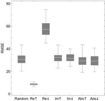
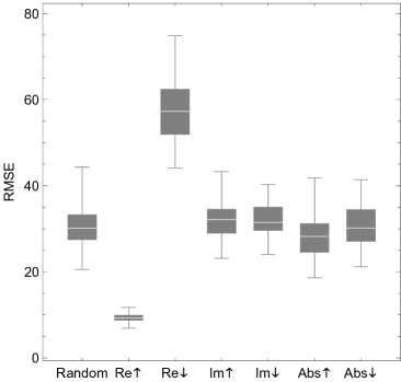
To address this issue, we have conducted numerical experiments with the following seven different heuristic criteria for sorting Laplacian eigenvalues of factor networks (while node strengths were always sorted in an ascending order):

1. Random

2. By real part (ascending)

3. By real part (descending)

4. By imaginary part (ascending)

5. By imaginary part (descending)

6. By absolute value (ascending)

7. By absolute value (descending)

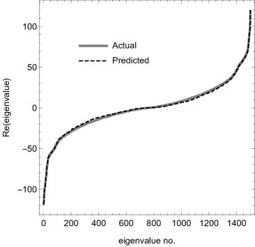
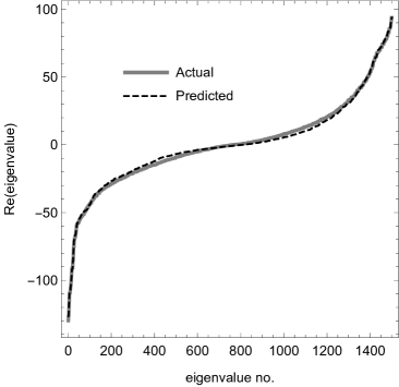
Results are summarized in Fig. 2. The results clearly show that, when the eigenvalues of Laplacian matrices of factor networks are sorted by their real parts in an ascending order (which is the most natural generalization of the sorting method used in [9]), the same methods described in Section 2 can approximate in- and out-strength Laplacian spectra of nonsimple DP/SPMNs most effectively. Examples of approximations are shown in Fig. 3.

(a) DPMNs	(b) SPMNs

Figure 2: Comparison of approximation performance among seven heuristic eigenvalue-sorting criteria (see text for details) for approximating in-strength Laplacian spectra of nonsimple (a) DPMNs and (b) SPMNs. “$\uparrow$” and “$\downarrow$” denote ascending and descending orders, respectively. The root mean square error (RMSE) per eigenvalue was used as a performance metric, in which an error was measured by the absolute value of the difference between true and approximated eigenvalues. Results were collected from one hundred independent tests for each condition, and their distributions were shown in box-whisker plots. Two adjacency matrices of factor networks used were: $A_{G}=$ a random matrix whose entries were randomly sampled from a uniform distribution $[-1,1]$, and $A_{H}=$ a random matrix whose entries were randomly sampled from a uniform distribution $[-2,2]$. The sizes of $A_{G}$ and $A_{H}$ were randomly and independently set between 40 and 60. These parameter values were chosen arbitrarily just for illustrative purposes, while the overall trends of results were robust to parameter variations. ANOVA and Tukey/Bonferroni posthoc tests showed extremely significant differences among the conditions ($p=3.75\times 10^{-331}$ for DPMNs; $p=2.13\times 10^{-324}$ for SPMNs). Results for out-strength Laplacian spectra showed similar trends.

(a) DPMN	(b) SPMN

Figure 3: Examples of in-strength Laplacian spectra of (a) a nonsimple DPMN and (b) a nonsimple SPMN, each approximated using the same methods as described in Section 2 [9] (black dashed curves), in comparison with the actual ones (gray solid curves). Eigenvalues are sorted by their real parts in an ascending order, and only their real parts are plotted (while imaginary parts were more or less randomly distributed). Two adjacency matrices of factor networks used were: $A_{G}=$ a $50\times 50$ random matrix whose entries were randomly sampled from a uniform distribution $[-1,1]$, and $A_{H}=$ a $30\times 30$ random matrix whose entries were randomly sampled from a uniform distribution $[-2,2]$. These parameter values were chosen arbitrarily just for illustrative purposes, while the overall trends of results were robust to parameter variations. Following the results shown in Fig. 2, the factor networks’ node strengths and Laplacian eigenvalues were sorted in ascending order (by their real parts for the latter) before the approximation method was used.

To summarize, the extension of GPMNs to nonsimple networks can be done in a straightforward manner, and the known spectral relationships between GPMNs and their factor networks are also applicable to nonsimple ones with little to no modification.

4 Generalizing Graph Product

The second extension being made in this paper is to generalize graph product operation to arbitrary linear combination of Cartesian and direct products. Specifically, we define the following generalized product:

Generalized product $\displaystyle G\operatorname*{\boxtimes}_{\alpha,\beta}H$

A network that is obtained as a weighted linear combination of $G\operatorname*{\Box}H$ and $G\operatorname*{\times}H$, where $\alpha$ and $\beta$ are used as weights. Its adjacency matrix is given by

$$A_{G\operatorname*{\boxtimes}_{\alpha,\beta}H}=A_{G}\operatorname*{\mathrlap{\oplus}\otimes}_{\alpha,\beta}A_{H}=\alpha A_{G}\operatorname*{\oplus}A_{H}+\beta A_{G}\operatorname*{\otimes}A_{H},$$ (4)

where the symbol $\displaystyle\operatorname*{\mathrlap{\oplus}\otimes}_{\alpha,\beta}$ is newly introduced in this paper to represent a weighted sum of the Kronecker sum and product. This graph product operation is still commutative and associative. All of CP/DP/SPMNs can be described uniformly using this generalized product ($\displaystyle\operatorname*{\boxtimes}_{1,0}=\operatorname*{\Box}$, $\displaystyle\operatorname*{\boxtimes}_{0,1}=\operatorname*{\times}$, and $\displaystyle\operatorname*{\boxtimes}_{1,1}=\operatorname*{\boxtimes}$). Moreover, setting $\alpha$ and/or $\beta$ to non-integer values represents a more nuanced balance between Cartesian and direct products in the GPMN structure (note that this is made possible by the first extension). We call networks generated by using this generalized product generalized GPMNs (GGPMNs).

We have found that the strength (degree), adjacency, and Laplacian spectra of GGPMNs can be given exactly or approximately as follows:

In- and out-strength spectra (= in- and out-strength sequence)

With $\left(d^{G}_{i}\right)$ and $\left(d^{H}_{j}\right)$ being the in- or out-strength spectra (node strengths) of factor networks $G$ and $H$, respectively:

GGPMN

$\left(\alpha d^{G}_{i}+\alpha d^{H}_{j}+\beta d^{G}_{i}d^{H}_{j}\right)$    $\forall i,j$

Adjacency spectra

With $\left(\lambda^{G}_{i}\right)$ and $\left(\lambda^{H}_{j}\right)$ being the adjacency spectra (eigenvalues of adjacency matrices) of factor networks $G$ and $H$, respectively:

GGPMN

$\left(\alpha\lambda^{G}_{i}+\alpha\lambda^{H}_{j}+\beta\lambda^{G}_{i}\lambda^{H}_{j}\right)$    $\forall i,j$

Approximated Laplacian spectra

With $\left[\left(d^{G}_{i}\right),\left(\mu^{G}_{i}\right)\right]$ and $\left[\left(d^{H}_{j}\right),\left(\mu^{H}_{j}\right)\right]$ being the in- or out-strength/Laplacian spectra of factor networks $G$ and $H$, respectively (all spectra should be sorted in an ascending order of real parts for best approximation):

GGPMN

$\left(\alpha\mu^{G}_{i}+\alpha\mu^{H}_{j}+\beta\mu^{G}_{i}d^{H}_{j}+\beta d^{G}_{i}\mu^{H}_{j}-\beta\mu^{G}_{i}\mu^{H}_{j}\right)$    $\forall i,j$

Details of derivation are given in Appendix. Note that these spectral relationships described in this section hold for both simple and nonsimple GGPMNs.

With these two extensions introduced in Sections 3 and 4, GPMNs as a modeling framework have gained an enhanced expressive power and can be used to describe a wider variety of complex networks. In the following sections, we illustrate the use of GPMNs through three application examples.

5 Application I: Predicting Epidemic Thresholds

GPMNs can be used to predict epidemic thresholds (i.e., critical ratio of infection and recovery rates) of epidemic processes on networks. It is known that the epidemic threshold is given by the reciprocal of the largest eigenvalue of the adjacency matrix of the network [12]. If the network can be modeled as a GGPMN, the largest eigenvalue of its adjacency matrix can be obtained analytically as

$$\lambda_{\max}^{G\operatorname*{\boxtimes}_{\alpha,\beta}H}=\max_{i,j}\left(\alpha\lambda^{G}_{i}+\alpha\lambda^{H}_{j}+\beta\lambda^{G}_{i}\lambda^{H}_{j}\right).$$ (5)

In most cases, the adjacency spectrum of a large simple graph is characterized by a dense area around the origin accompanied by a small number of substantially larger (positive) outliers [13]. Therefore, if $\alpha\geq 0$ and $\beta\geq 0$, Eq. (5) is simplified to

$$\lambda_{\max}^{G\operatorname*{\boxtimes}_{\alpha,\beta}H}=\alpha\lambda^{G}_{\max}+\alpha\lambda^{H}_{\max}+\beta\lambda^{G}_{\max}\lambda^{H}_{\max}.$$ (6)

Because the epidemic threshold is the reciprocal of the largest eigenvalue, this result indicates that the epidemic threshold on a CPMN ($(\alpha,\beta)=(1,0)$) is twice the harmonic mean of the thresholds on two factor networks. Similarly, the epidemic threshold on a DPMN ($(\alpha,\beta)=(0,1)$) is simply the product of the thresholds on two factor networks.

A particularly interesting application of this result is the prediction of epidemic thresholds on random networks generated by a stochastic block model with equal community size. Let $P$ be an $r\times r$ edge probability matrix, and assume each community is made of exactly $m$ nodes (thus the total number of nodes is $rm$). Then, the ensemble average of adjacency matrices of networks generated by this model is given by $P\operatorname*{\otimes}R$, an adjacency matrix of a nonsimple DPMN, where $R$ is an $m\times m$ all-one square matrix. A typical assumption in matrix perturbation theory suggests that the spectrum of a specific binary adjacency matrix generated from this stochastic block model behaves similarly with the spectrum of this ensemble average. Therefore, we can estimate the epidemic threshold on a random network generated with this model by calculating the largest eigenvalue of $P\operatorname*{\otimes}R$. Since $R$ has $m$ as the single largest eigenvalue (while all other eigenvalues are 0s), this estimation becomes as simple as

$$\lambda_{\max}^{P\operatorname*{\otimes}R}=\lambda^{P}_{\max}m.$$ (7)

This accomplishes a significant reduction of computational cost because the number of communities (size of $P$) is usually significantly smaller than the size of the entire network. Figure 4 presents results of a numerical experiment that compared the estimated largest eigenvalues obtained using this method with the actual ones, showing excellent matching between the two.

Figure 4: Comparison of estimated and actual largest eigenvalues of adjacency matrices of random networks generated by a stochastic block model. Results were collected from five hundred independent calculations. In each case, the number of communities ($r$) and the size of each community ($m$) were randomly chosen between 3 and 7 and between 40 and 60, respectively. These parameter values were chosen arbitrarily just for illustrative purposes, while the overall trends of results were robust to parameter variations. $P$ and an actual binary adjacency matrix were randomly generated to be symmetric in each case. The estimated values were calculated using Eq. (7), while the actual ones were explicitly computed from the binary adjacency matrices.

We note that other recent studies also discuss spectral properties of stochastic block models, mainly from the viewpoint of community detectability [14, 15, 16]. Compared to them, the example presented in this section above is unique in using graph product as a concise mathematical representation of network topology and focusing specifically on the prediction of epidemic thresholds.

6 Application II: Propagation in Nontrivial Space and Time

GPMNs can be used to represent dynamical processes taking place in nontrivial spatial and/or temporal structures. A popular way of doing this is to use one of the factor networks as a network-shaped spatial structure, while the other as an identical dynamical network that is embedded inside of each node in space. There are several such multilayer network models developed and used in the literature, including coupled cellular networks [17] and ecological networks on interconnected habitats [8]. In these cases, network topologies that can be produced by Cartesian products were typically used to couple multiple identical intra-layer networks over space.

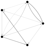
Here, we illustrate other uses of GPMNs to represent dynamical processes that involve not just nontrivial space but also time. Specifically, we use graph product to represent various types of weighted random walks on a network. Let $G$ be a weighted, directed network that represents transition likelihoods, and $T$ a chain made of directed edges (Fig. 5, top). Each of these networks in isolation can be considered a representation of either spatial movement without time ($G$), or the flow of time without spatial movement ($T$). Applying different graph product operators to these two factor networks produces a specific spatio-temporal representation of different random walk processes, as follows:

$G$ :
$T$ :

(a) $G\operatorname*{\times}T$ :

(b) $G\operatorname*{\Box}T$ :

(c) $\displaystyle G\operatorname*{\boxtimes}_{\alpha,\beta}T$ :

Figure 5: Weighted random walk processes represented by GPMNs. Top: Two factor networks. $G$ represents an underlying spatial transition network, while $T$ represents time. (a) Direct product $G\operatorname*{\times}T$, representing random walk with forced temporal progress. (b) Cartesian product $G\operatorname*{\Box}T$, representing random walk within each time segment with occasional stochastic temporal progress. (c) Generalized product $\displaystyle G\operatorname*{\boxtimes}_{\alpha,\beta}T$, representing the combination of (a) and (b). Circles represent layers (time segments).

Direct product $G\operatorname*{\times}T$

This represents weighted random walk with forced temporal progress (Fig. 5(a)). Each layer contains no intra-layer edges, and all the edges connect a node in one layer to another node in the subsequent layer, indicating that no entities can stay within the same time point when they make transitions. This is the most natural representation of “vanilla” random walk in which time is explicitly represented by $T$.

Cartesian product $G\operatorname*{\Box}T$

This represents weighted random walk taking place within each time segment (layer) with occasional stochastic temporal progress without spatial transition (Fig. 5(b)). Each layer contains the original $G$ as is, while all the inter-layer edges are diagonal, i.e., connecting the same node from one time point to the next. The relative probability of such temporal progress can be adjusted by changing the average edge weight in $T$ (we call it $\langle E_{T}\rangle$) with reference to the average edge weight in $G$ (we call it $\langle E_{G}\rangle$). This can be a useful random walk model if time has well-defined segments (e.g., days, weeks, months) and many transitions are expected to occur within each segment before moving onto the next segment.

Generalized product $\displaystyle G\operatorname*{\boxtimes}_{\alpha,\beta}T$

This represents the combination of the above two random walk processes with their relative weights given by $\alpha$ and $\beta$ (Fig. 5(c)). Therefore, together with the $\langle E_{T}\rangle/\langle E_{G}\rangle$ ratio, this model essentially has three adjustable global parameters. They collectively determine the relative likelihoods of (i) transitions within a single time segment (determined by $\alpha\langle E_{G}\rangle$), (ii) temporal progress without spatial transitions (determined by $\alpha\langle E_{T}\rangle$), and (iii) temporal progress with spatial transitions (determined by $\beta\langle E_{G}\rangle\langle E_{T}\rangle$).

Using this framework, interactions between nontrivial space and time in the propagation processes can be written concisely, and the spectral properties of the resulting GPMN can be obtained analytically (or by approximation for Laplacian spectra when a non-Cartesian product is used). To the best of our knowledge, such use of graph product to represent interactions between nontrivial space and time is novel in the literature.

For example, consider a random spreading process on a network occurring in a cyclical time structure (e.g., a seasonal cycle in a year), where $G$ is a typical transition probability matrix and $T$ is a directed circular graph. Applying any of the above graph product operators to these two factor networks produces a nonsimple GPMN model of a weighted random walk process developing in both space and time. The largest eigenvalue of the resulting adjacency matrix, an indicator of the efficiency of spreading (and persistence), can still be predicted using Eqs. (5) or (6). If $\lambda^{G}_{\max}$ is assumed to be constant, the efficiency of spreading is solely determined by the adjacency spectrum of $T$.

(a)	(b)

Figure 6: Dependence of $\lambda_{\max}$ (spreading efficiency) on $\tau$ (number of months to which resource is invested), analytically obtained from adjacency spectra of factor networks using Eq. (6). The interactions between space and time was represented by a generalized product $G\operatorname*{\boxtimes}_{0.5,0.5}T$, where $G$ is a $1000\times 1000$ random transition probability matrix (fixed) and $T$ is a directed circular graph made of 12 nodes, representing 12 months = 1 year. Edge weights in $T$ were determined based on the investment strategy, described below. (a) Results from the epidemic control scenario, in which the default edge weight in $T$ was 1, and $\tau$ randomly selected edges in $T$ received a $C/\tau$ weight reduction each. (b) Results from the marketing scenario, in which the default edge weight in $T$ was $10^{-3}$, and $\tau$ randomly selected edges in $T$ received a $C/\tau$ weight increase each.

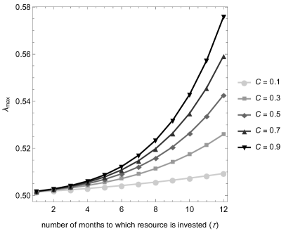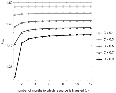
This model provides implications for temporal investment strategies for epidemic control or marketing. In an epidemic control scenario, it is reasonable to assume that $T$ has a large edge weight by default and one needs to allocate a finite resource (denoted as $C$) to reduce some (or all) of edge weights to suppress continuation of a disease from one time point to another. In a marketing scenario, however, the situation would be nearly the opposite; the default edge weight in $T$ is assumed to be near-zero and one needs to allocate the resource to increase the chance of retention of product adoption over time. Temporally heterogeneous investment strategies can be efficiently represented by varying edge weights in $T$, and the spreading efficiency (the largest eigenvalue of the entire adjacency matrix of the GPMN) can be obtained efficiently using its spectral properties. Figure 6 presents a sample result of such numerical computation for $G$ with 1000 nodes and $T$ with 12 nodes (time segments), clearly showing that temporally concentrated investment was most effective for epidemic control, but temporally distributed investment was necessary for marketing.

7 Application III: Higher-Order Properties

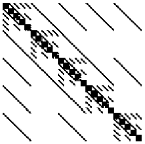
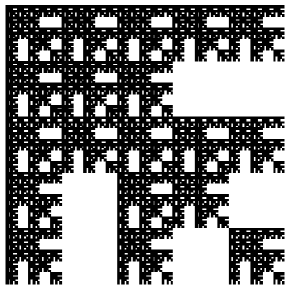
Lastly, we discuss a rather different type of application of GPMNs: higher-order powers of a network. Because graph product operators we have considered are all associative, we can create GPMNs by raising a network to the power of $n$ using any of the operators, such as $G\operatorname*{\Box}G\operatorname*{\Box}G\operatorname*{\Box}\ldots\operatorname*{\Box}G=G^{n}_{\operatorname*{\Box}}$ (and similarly, $G^{n}_{\operatorname*{\times}}$, $G^{n}_{\operatorname*{\boxtimes}}$, etc.). We call these GPMNs self-similar GPMNs, because their inter-layer structures are similar to their intra-layer structures, and also because their adjacency and Laplacian matrices asymptotically become fractal matrices (Fig. 7) as the power $n$ increases.

(a)	(b)

Figure 7: Examples of adjacency and Laplacian matrices of self-similar GPMNs of a higher-order power, showing fractal structure. The original network $G$ was a random graph with 5 nodes and 7 edges. (a) Adjacency matrix of $G^{5}_{\operatorname*{\Box}}$. (b) Laplacian matrix of $G^{5}_{\operatorname*{\boxtimes}}$. Non-zero elements are visualized with black pixels.

We can analytically predict spectral distributions of self-similar GPMNs for certain cases, as follows:

$G^{n}_{\operatorname*{\Box}}(\alpha=1,\beta=0)$

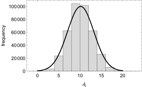
In this case, all the degree/strength, adjacency, and Laplacian spectra will be given by the sums of $n$ sample values independently selected (repetition allowed) from the original spectrum of $G$, to which the central limit theorem applies. Therefore, with $n\to\infty$, the asymptotic spectral distribution of $G^{n}_{\operatorname*{\Box}}$ will approach a normal distribution with mean $\langle x\rangle n$ and standard deviation $\sigma_{x}\sqrt{n}$, where $\langle x\rangle$ and $\sigma_{x}$ are the mean and the standard deviation of the original spectrum, respectively. The smallest and largest values will also scale linearly with $n$.

$G^{n}_{\operatorname*{\times}}(\alpha=0,\beta=1)$

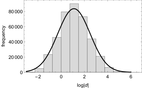
In this case, the degree/strength and adjacency spectra will be given by the products of $n$ sample values independently selected (repetition allowed) from the original spectrum of $G$. The adjacency spectrum may contain negative or even complex numbers (if $G$ is directed). However, if we take the logarithms of their absolute values, this again becomes the sums of $n$ sample values, to which the central limit theorem still applies. Therefore, with $n\to\infty$, the asymptotic distribution of absolute values of the degree/strength and adjacency spectra of $G^{n}_{\operatorname*{\times}}$ will approach a log-normal distribution (with mean $\langle\log|x|\rangle n$ and standard deviation $\sigma_{\log|x|}\sqrt{n}$ in log space). The smallest and largest absolute values will scale exponentially with $n$.

$G^{n}_{\operatorname*{\boxtimes}}(\alpha=1,\beta=1)$

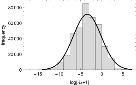
In this case, the degree/strength and adjacency spectra will be given by the same formula $\left(x_{i}+x_{j}+x_{i}x_{j}\right)=\left((x_{i}+1)(x_{j}+1)-1\right)$ $\forall i,j$. The right hand side contains convenient $+1$ and $-1$, which indicates that distributions obtained by elevating all values in these spectra by 1 will behave exactly the same way as the degree/strength and adjacency spectra of $G^{n}_{\operatorname*{\times}}$ discussed right above. Therefore, with $n\to\infty$, the asymptotic distribution of absolute values of the degree/strength and adjacency spectra of $G^{n}_{\operatorname*{\boxtimes}}$, when elevated by 1, will approach a log-normal distribution (with mean $\langle\log|x+1|\rangle n$ and standard deviation $\sigma_{\log|x+1|}\sqrt{n}$ in log space). The smallest and largest absolute values (after elevated by 1) will scale exponentially with $n$.

Figure 8 presents some examples of spectral distributions of self-similar GPMNs together with analytical predictions described above. Analytical predictions showed a good fit to the actual spectral distributions.

(a)

(b)

(c)

Figure 8: Comparison of spectral distributions of self-similar GPMNs (histograms) and analytical predictions (curves). In all cases, the original network $G$ was a random network with 5 nodes and 7 edges, and each edge was assigned a random weight. (a) Laplacian spectrum of $G^{8}_{\operatorname*{\Box}}$. (b) Strength spectrum of $G^{8}_{\operatorname*{\times}}$. (c) Adjacency spectrum of $G^{8}_{\operatorname*{\boxtimes}}$.

An illustrative example of application of self-similar GPMNs to dynamical networks is to use self-similar DPMNs to represent simultaneous Markov processes on a network. Specifically, the $n$-th power of a state transition network (such as $G$ given in Fig. 5), when raised by direct product, gives a higher-order transition network for meta-states of a population of $n$ independent yet distinguishable Markovian individuals. This can be easily understood in that each of the nodes of this self-similar DPMN is a composite of $n$ independent choices of states in the original transition network, and that the state transition probabilities between those composite nodes are given by the $n$-th power (by Kronecker product) of the original transition probability matrix, i.e., the transition probability between two composite states is a simple product of $n$ independent transition probabilities between original individual states. This represents $n$ identical, independent, simultaneous Markovian processes taking place on a network, using a higher-order algebraic notation.

The results given in this section indicate that it is possible to analytically predict some of the dynamical properties of systems represented in self-similar GPMNs, including the simultaneous Markov processes described above. We can characterize the spectral density function and the scaling behavior of the largest/smallest values (in either original values or in their absolute values). In particular, the dominant eigenvalue of a self-similar GPMN is most likely determined solely by the dominant eigenvalues of the original network. Meanwhile, the fact that the spectra will approach a normal or log-normal distribution implies that the less dominant modes of the network’s collective states will behave more and more homogeneously as the order increases.

Finally, self-similar GPMNs can also be used to predict spectral properties of certain high-dimensional networks of mathematical interest. For example, an $n$-dimensional hypercube can be considered a self-similar CPMN of a complete graph made of two nodes, raised to the $n$-th power using Cartesian product. We can easily predict that a high-dimensional hypercube’s adjacency and Laplacian spectra will asymptotically become a normal distribution centered at the origin and at $n$, respectively, because the adjacency and Laplacian spectra of the original two-node graph have $0$ and $1$ as their means, respectively. This agrees with the results recently reported elsewhere [18].

8 Conclusions

We have discussed GPMNs and their spectral properties. With the two extensions introduced in this paper, GPMNs form an interesting, useful family of multilayer networks that can provide an efficient, analytically tractable framework for describing certain classes of complex networks. GPMNs show mathematically nice behaviors in a number of aspects, which can facilitate analytical and computational investigation of structure and dynamics of various multilayer networks. We also have presented several examples of applications, which, we hope, have collectively illustrated the effectiveness and practical value of the GPMN framework.

As mentioned earlier in Section 1, it would be highly unlikely that the structure and dynamics of a real-world network could be perfectly captured within the GPMN framework. While this is certainly a limitation of GPMNs, it also suggests different roles for GPMNs to play in the science of complex networks. Specifically, with their simplicity and mathematically nice behavior, GPMNs may serve as an analytically tractable approximation model, with which researchers can produce analytical predictions and/or systematic comparison and testing of empirically observed properties of multilayer networks. This is similar to what mean-field models have been offering to high-dimensional dynamical systems analysis. We believe that GPMNs can contribute to the multilayer networks literature in a similar manner.

There are a number of directions of further research. The approximation of Laplacian spectra of DP/SP/GGPMNs requires further development in both mathematical justification and performance improvement. The three areas of applications should be evaluated through more testing and validation using real-world network data. There are also much room for further theoretical development and exploration. For example, the implications of spectral properties of GPMNs for canonical dynamical network models (e.g., diffusion, synchronization, opinion formation, etc.) deserves more elaboration. Another intriguing area of investigation would be the use of nonlinear time structure, such as non-deterministic (branching) flow of time, as a factor network in the spatio-temporal interaction modeling, to explore other applications of GPMNs in different fields of physics and computer science. Possible connections between large-scale stochastic dynamics and GPMNs may also be worth further investigation.

Funding

This work was supported by the Visitors Program of the Max Planck Institute for the Physics of Complex Systems.

Appendix: Spectral Relationships Between GGPMNs and Their Factor Networks

Here we show that the strength (degree) and adjacency spectra of GGPMNs still maintain exact algebraic relationships with those of their factor networks, as follows:

In-strength spectra (= in-strength sequence)

With $\left(d^{G}_{i}\right)$ and $\left(d^{H}_{j}\right)$ being the node strengths of factor networks $G$ and $H$, respectively:

$$\left(d^{G\operatorname*{\boxtimes}_{\alpha,\beta}H}\right) =\left(A_{G}\operatorname*{\mathrlap{\oplus}\otimes}_{\alpha,\beta}A_{H}\right)\mathbbm{1}_{|V_{G}||V_{H}|}=\left(\alpha A_{G}\operatorname*{\oplus}A_{H}+\beta A_{G}\operatorname*{\otimes}A_{H}\right)\left(\mathbbm{1}_{|V_{G}|}\operatorname*{\otimes}\mathbbm{1}_{|V_{H}|}\right)$$ (8)

$$=\alpha\left(A_{G}\operatorname*{\otimes}I_{|V_{H}|}\right)\left(\mathbbm{1}_{|V_{G}|}\operatorname*{\otimes}\mathbbm{1}_{|V_{H}|}\right)+\alpha\left(I_{|V_{G}|}\operatorname*{\otimes}A_{H}\right)\left(\mathbbm{1}_{|V_{G}|}\operatorname*{\otimes}\mathbbm{1}_{|V_{H}|}\right)+\beta\left(A_{G}\operatorname*{\otimes}A_{H}\right)\left(\mathbbm{1}_{|V_{G}|}\operatorname*{\otimes}\mathbbm{1}_{|V_{H}|}\right)$$ (9)

$$=\alpha\left(d^{G}\right)\operatorname*{\otimes}\mathbbm{1}_{|V_{H}|}+\alpha\mathbbm{1}_{|V_{G}|}\operatorname*{\otimes}\left(d^{H}\right)+\beta\left(d^{G}\right)\operatorname*{\otimes}\left(d^{H}\right)$$ (10)

$$=\underline{\left(\alpha d^{G}_{i}+\alpha d^{H}_{j}+\beta d^{G}_{i}d^{H}_{j}\right)}\quad\quad\forall i,j$$ (11)

Out-strength spectra can be obtained similarly by the same formula.

Adjacency spectra

With $\left(\lambda^{G}_{i},v^{G}_{i}\right)$ and $\left(\lambda^{H}_{j},v^{H}_{j}\right)$ being eigenvalues and eigenvectors of $A_{G}$ and $A_{H}$, respectively:

$$A_{G\operatorname*{\boxtimes}_{\alpha,\beta}H}\left(v^{G}_{i}\operatorname*{\otimes}v^{H}_{j}\right) =\left(A_{G}\operatorname*{\mathrlap{\oplus}\otimes}_{\alpha,\beta}A_{H}\right)\left(v^{G}_{i}\operatorname*{\otimes}v^{H}_{j}\right)=\left(\alpha A_{G}\operatorname*{\oplus}A_{H}+\beta A_{G}\operatorname*{\otimes}A_{H}\right)\left(v^{G}_{i}\operatorname*{\otimes}v^{H}_{j}\right)$$ (12)

$$=\alpha\left(A_{G}\operatorname*{\otimes}I_{|V_{H}|}\right)\left(v^{G}_{i}\operatorname*{\otimes}v^{H}_{j}\right)+\alpha\left(I_{|V_{G}|}\operatorname*{\otimes}A_{H}\right)\left(v^{G}_{i}\operatorname*{\otimes}v^{H}_{j}\right)+\beta\left(A_{G}\operatorname*{\otimes}A_{H}\right)\left(v^{G}_{i}\operatorname*{\otimes}v^{H}_{j}\right)$$ (13)

$$=\alpha\left(\lambda^{G}_{i}v^{G}_{i}\right)\operatorname*{\otimes}v^{H}_{j}+\alpha v^{G}_{i}\operatorname*{\otimes}\left(\lambda^{H}_{j}v^{H}_{j}\right)+\beta\left(\lambda^{G}_{i}v^{G}_{i}\right)\operatorname*{\otimes}\left(\lambda^{H}_{j}v^{H}_{j}\right)$$ (14)

$$=\underline{\left(\alpha\lambda^{G}_{i}+\alpha\lambda^{H}_{j}+\beta\lambda^{G}_{i}\lambda^{H}_{j}\right)}\left(v^{G}_{i}\operatorname*{\otimes}v^{H}_{j}\right)\quad\quad\forall i,j$$ (15)

Moreover, we present that the Laplacian spectra of GGPMNs can also be approximated using the strength (degree) and Laplacian spectra of their factor networks, as follows:

Approximated Laplacian spectra

With $\left(\mu^{G}_{i},w^{G}_{i}\right)$ and $\left(\mu^{H}_{j},w^{H}_{j}\right)$ being eigenvalues and eigenvectors of in- or out-strength Laplacian matrices of $G$ ($L_{G}$) and $H$ ($L_{H}$), respectively, and $\left(w^{G}_{i}\operatorname*{\otimes}w^{H}_{j}\right)$ being used as pseudo-eigenvectors of $L_{G\operatorname*{\boxtimes}_{\alpha,\beta}H}$ [9]:

$$L_{G\operatorname*{\boxtimes}_{\alpha,\beta}H}\left(w^{G}_{i}\operatorname*{\otimes}w^{H}_{j}\right) =\left(D_{G\operatorname*{\boxtimes}_{\alpha,\beta}H}-A_{G\operatorname*{\boxtimes}_{\alpha,\beta}H}\right)\left(w^{G}_{i}\operatorname*{\otimes}w^{H}_{j}\right)$$ (16)

$$=\left(\alpha D_{G\operatorname*{\Box}H}+\beta D_{G\operatorname*{\times}H}-\alpha A_{G\operatorname*{\Box}H}-\beta A_{G\operatorname*{\times}H}\right)\left(w^{G}_{i}\operatorname*{\otimes}w^{H}_{j}\right)$$ (17)

$$=\left(\alpha D_{G}\operatorname*{\otimes}I_{|V_{H}|}+\alpha I_{|V_{G}|}\operatorname*{\otimes}D_{H}+\beta D_{G}\operatorname*{\otimes}D_{H}-\alpha A_{G}\operatorname*{\otimes}I_{|V_{H}|}-\alpha I_{|V_{G}|}\operatorname*{\otimes}A_{H}-\beta A_{G}\operatorname*{\otimes}A_{H}\right)$$

$$\quad\quad\left(w^{G}_{i}\operatorname*{\otimes}w^{H}_{j}\right)$$ (18)

$$=\left[\alpha L_{G}\operatorname*{\otimes}I_{|V_{H}|}+\alpha I_{|V_{G}|}\operatorname*{\otimes}L_{H}+\beta D_{G}\operatorname*{\otimes}D_{H}-\beta\left(D_{G}-L_{G}\right)\operatorname*{\otimes}\left(D_{H}-L_{H}\right)\right]\left(w^{G}_{i}\operatorname*{\otimes}w^{H}_{j}\right)$$ (19)

$$=\left(\alpha L_{G}\operatorname*{\otimes}I_{|V_{H}|}+\alpha I_{|V_{G}|}\operatorname*{\otimes}L_{H}+\beta L_{G}\operatorname*{\otimes}D_{H}+\beta D_{G}\operatorname*{\otimes}L_{H}-\beta L_{G}\operatorname*{\otimes}L_{H}\right)\left(w^{G}_{i}\operatorname*{\otimes}w^{H}_{j}\right)$$ (20)

$$=\alpha\left(\mu^{G}_{i}w^{G}_{i}\right)\operatorname*{\otimes}w^{H}_{j}+\alpha w^{G}_{i}\operatorname*{\otimes}\left(\mu^{H}_{j}w^{H}_{j}\right)+\beta\left(\mu^{G}_{i}w^{G}_{i}\right)\operatorname*{\otimes}\left(D_{H}w^{H}_{j}\right)+\beta\left(D_{G}w^{G}_{i}\right)\operatorname*{\otimes}\left(\mu^{H}_{j}w^{H}_{j}\right)$$

$$\quad\quad-\beta\left(\mu^{G}_{i}w^{G}_{i}\right)\operatorname*{\otimes}\left(\mu^{H}_{j}w^{H}_{j}\right)$$ (21)

$$\approx\underline{\left(\alpha\mu^{G}_{i}+\alpha\mu^{H}_{j}+\beta\mu^{G}_{i}d^{H}_{j}+\beta d^{G}_{i}\mu^{H}_{j}-\beta\mu^{G}_{i}\mu^{H}_{j}\right)}\left(w^{G}_{i}\operatorname*{\otimes}w^{H}_{j}\right)\quad\quad\forall i,j$$ (22)

(with heuristic assumptions $$D_{G}w^{G}_{i}\approx d^{G}_{i}w^{G}_{i} D_{H}w^{H}_{j}\approx d^{H}_{j}w^{H}_{j}$$ and [9])

We have conducted similar numerical experiments as in Section 3 to confirm that sorting eigenvalues of factor networks’ Laplacian matrices by their real parts in an ascending order is still most effective for approximation of GGPMNs’ Laplacian spectra (results not shown, as they were quite similar to Fig. 2).

Note that these spectral relationships described in this appendix hold for both simple and nonsimple GGPMNs.

References

- [1] Mikko Kivelä, Alex Arenas, Marc Barthelemy, James P Gleeson, Yamir Moreno, and Mason A Porter. Multilayer networks. Journal of Complex Networks, 2(3):203–271, 2014.
- [2] Stefano Boccaletti, G Bianconi, R Criado, Charo I Del Genio, J Gómez-Gardeñes, M Romance, I Sendina-Nadal, Z Wang, and M Zanin. The structure and dynamics of multilayer networks. Physics Reports, 544(1):1–122, 2014.
- [3] Manlio De Domenico, Clara Granell, Mason A Porter, and Alex Arenas. The physics of spreading processes in multilayer networks. Nature Physics, 12:901–906, 2016.
- [4] Jure Leskovec, Deepayan Chakrabarti, Jon Kleinberg, Christos Faloutsos, and Zoubin Ghahramani. Kronecker graphs: An approach to modeling networks. The Journal of Machine Learning Research, 11:985–1042, 2010.
- [5] Albert Solé-Ribalta, Manlio De Domenico, Nikos E Kouvaris, Albert Díaz-Guilera, Sergio Gómez, and Alex Arenas. Spectral properties of the Laplacian of multiplex networks. Physical Review E, 88(3):032807, 2013.
- [6] Manlio De Domenico, Albert Solé-Ribalta, Emanuele Cozzo, Mikko Kivelä, Yamir Moreno, Mason A Porter, Sergio Gómez, and Alex Arenas. Mathematical formulation of multilayer networks. Physical Review X, 3(4):041022, 2013.
- [7] Malbor Asllani, Daniel M Busiello, Timoteo Carletti, Duccio Fanelli, and Gwendoline Planchon. Turing instabilities on Cartesian product networks. Scientific Reports, 5(12927), 2015.
- [8] Andreas Brechtel, Philipp Gramlich, Daniel Ritterskamp, Barbara Drossel, and Thilo Gross. Master stability functions reveal diffusion-driven instabilities in multi-layer networks. arXiv preprint arXiv:1610.07635, 2016.
- [9] Hiroki Sayama. Estimation of Laplacian spectra of direct and strong product graphs. Discrete Applied Mathematics, 205:160–170, 2016.
- [10] Cyrus Colton MacDuffee. The Theory of Matrices. Springer-Verlag, 1933.
- [11] Miroslav Fiedler. Algebraic connectivity of graphs. Czechoslovak Mathematical Journal, 23(2):298–305, 1973.
- [12] Deepayan Chakrabarti, Yang Wang, Chenxi Wang, Jurij Leskovec, and Christos Faloutsos. Epidemic thresholds in real networks. ACM Transactions on Information and System Security (TISSEC), 10(4):13, 2008.
- [13] Illes J Farkas, Imre Derényi, Albert-László Barabási, and Tamas Vicsek. Spectra of greal-world h graphs: Beyond the semicircle law. Physical Review E, 64(2):026704, 2001.
- [14] Raj Rao Nadakuditi and Mark EJ Newman. Graph spectra and the detectability of community structure in networks. Physical Review Letters, 108(18):188701, 2012.
- [15] Tiago P Peixoto. Eigenvalue spectra of modular networks. Physical Review Letters, 111(9):098701, 2013.
- [16] Amir Ghasemian, Pan Zhang, Aaron Clauset, Cristopher Moore, and Leto Peel. Detectability thresholds and optimal algorithms for community structure in dynamic networks. Physical Review X, 6(3):031005, 2016.
- [17] Martin Golubitsky and Reiner Lauterbach. Bifurcations from synchrony in homogeneous networks: Linear theory. SIAM Journal on Applied Dynamical Systems, 8(1):40–75, 2009.
- [18] Stanley F Florkowski. Spectral graph theory of the hypercube. Master’s thesis, Monterey, California. Naval Postgraduate School, 2008.