To Vojislav Golo…
Computation of effective electrical conductivity of composite materials: a novel approach based on analysis of graphs.
Abstract
In this work we continue the investigation of different approaches to conception and modeling of composite materials. The global method we focus on, is called ’stochastic homogenization’. In this approach, the classical deterministic homogenization techniques and procedures are used to compute the macroscopic parameters of a composite starting from its microscopic properties. The stochastic part is due to averaging over some series of samples, and the fact that these samples fit into the concept of RVE (Representative Volume Element) in order to reduce the variance effect.
In this article, we present a novel method for computation of effective electric properties of composites – it is based on the analysis of the connectivity graph (and the respective adjacency matrix) for each sample of a composite material. We describe how this matrix is constructed in order to take into account complex microscopic geometry. We also explain what we mean by homogenization procedure for electrical conductivity, and how the constructed matrix is related to the problem. The developed method is applied to a test study of the influence of micromorphology of composites materials on their conductivity.
I Introduction / motivation
Composite materials and more generally heterogeneous media appear in various real-life situations. The latter represent the matter from microscopic scale to perfectly observable macro objects, while the former play an important industrial role in the last decades. The incredibly fast development of composite materials in most of the branches of modern technology is due to their exceptional properties in comparison with pure materials. The process of conception and production of composites is however far from being simple: while a lot of tests are needed to be able to validate the technology before going to industrial applications, the experimental work is still expensive and not easy to carry out. All this results in a strong demand for efficient mathematical modelling techniques that can be applied to predict and optimize effective properties of composite materials. Moreover in the recent years computational facilities have become much more accessible, that resulted in a great number of works dealing with development of methods and implementation of algorithms for such studies111Similar logic goes far beyond the subject of composite materials: one can for example recall the Nobel Prize 2013 in chemistry, that was given more or less for advances in computer simulations.. Out of all possible approaches to the problem we focus on the method which is usually called stochastic homogenization.
The key idea of homogenization as a modelling technique222not to be confused with an industrial process is to be able to estimate measurable macroscopic parameters of a composite material (or heterogeneous medium) starting from its microscopic geometry. In a sense, one computes the parameters of an equivalent homogeneous material that can “replace” the studied heterogeneous medium in the experiment. Various techniques based on different mathematical and algorithmic approaches have been proposed. In what follows, we will see that it is very important to carefully choose suitable methods, and this choice is greatly influenced by the problem one is solving or by a property one is studying, and also by availability and type of the input data. In our previous papers we have observed for example, that the methods based on Fast Fourier Transform proposed initially in moul-suq ; monchiet for 2D problems, are perfectly suitable for studying elastic properties in 3D (VSPD ), but they have to be modified to be applied to thermal phenomena (SVDP2 ; SVDP3 ). It became clear from the previous studies (SVDP4 ) that they are practically not efficient to estimate electrical conductivity, which is the main motivation for the method we describe in this paper.
The stochastic part in the name of the method is due to the fact that each given sample of a medium does not capture exactly the behavior of the composite material. One is thus forced to average the results on a reasonable sampling with some common properties. The idea is coming from a very classical approach of Monte Carlo simulations. For our purposes, it means that an efficient algorithm of generation of such samples should be implemented. We profit from the flexibility of the methods we have developped in VDP ; SVDP to use them in the analysis of electrical conductivity.
Our interest in the subject is also motivated by some very concrete applications related to aeronautic equipment, a project carried out in close collaboration with industrial partners. Some part of this contribution will thus be devoted to explaining in what way the techniques can indeed be applied and to potential difficulties that arise in “true-to-life” situations, and to possible ways out.
The main goal of this paper is to provide a tool that can be applied “out of the box” in order to study effective properties of heterogeneous media or composite materials. Therefore we present the “building blocks” for such a tool, that are sufficiently flexible and can be then “assembled” depending on the available input data and the problem under consideration. For each method that is discussed here, we give ideas of some mathematical background, that is necessary for understand and application, we do not however go into much details not to overload the presentation.
To sum it up, the text is organized as follows: In the next section (II) we briefly recall the tools we have developped for generating samples of composite materials/heterogeneous media with rather complex microscopic geometry; we explain how they can be easily adapted to cover the situations arising typically in the studies of electrical conductivity. In the section III the novel (deterministic) homogenization procedure is presented – it is based on the analysis of the connectivity graph of a material and is perfectly suitable for the type of samples we produce. The last section (IV) is devoted to application of the developped method to some test examples, it also contains some discussion about its adaptation to industrial problems.
II Stochastic part – sample generation
A composite material, or what is the same in our analysis, a heterogeneous medium, is a material composed of several constituents often called phases. Typically one thinks about some “matrix”, say made of a polymer, into which inclusions of a different nature are inserted. For electrical conductivity the matrix would be made of an insulator (or a material with rather low conductivity) and inclusions would be microparticles chosen to conduct electricity (typically containing a metal/alloy or some other material with high conductivity). It is intuitively clear (and also confirmed by a lot of studies) that effective properties of composite materials strongly depend on the volume fraction of inclusions, but sometimes even in a more pronounced way on the morphology of the material, i.e. microgeometry and repartition of inclusions. For modelling, it is thus important to be able to generate samples that are close enough to the actual microstructure of the material. But since we talk about stochastic homogenization, i.e. averaging the results over a big series of tests, this process should not take too much time. Not going much into details, let us just say that the usual way out is to replace the inclusions by simple geometric objects and handle their repartition inside the sample. And certainly a lot of work has been done in this direction (see VDP ; SVDP and references therein).
The concrete tool we have at hand permits to place spherical and cylindrical inclusions into the matrix, that already gives a very rich “true-to-life” microscopic geometry. The key feature that we need throughout all the studies is the ability to control contacts and overlaps of inclusions. In the previous studies (elastic and thermal) we were rather focusing on non-overlapping or slightly overlapping inclusions – the machinery had been developped mostly for that. Let us be slightly more specific about the algorithm. There are essentially two methods how to generate samples with non-intersecting inclusions: RSA- and MD-based ones. RSA (rsa1 ) stands for “random sequential addition” – the inclusions are generated one after another, and only those that do not intersect with previously generated ones are kept. MD (LSA ) stands for “molecular dynamics” – all the inclusions are generated simultaneously, and then repulsive forces are introduced to position them correctly. Both algorithms have been adapted to the case of spherical and cylindrical inclusions and implemented in VDP . The input of the algorithms consists of the desired volume fraction, the respective number of spheres and cylinders and their geometric parameters. The output is a list of non-intersecting inclusions with coordinates of their centers and angles responsible for orientation, this can be used directly in computations or converted to a 3D image like figure 1.(a).
Let us note that the numbers should be chosen in order to fit the concept of a Representative Volume Element (RVE, kanit ): the sample should be large enough to effectively capture the properties of the material, like isotropy for example, but sufficiently small to make the computation doable. We have performed a detailed study of the effective elastic properties of composite materials in VSPD and it included also some tests to choose the size of the RVE. Let us just mention here that if the volume fraction and the proportion of each type of inclusions are fixed, the choice of the size of the RVE is governed by the number of inclusions. The usual way to determine this number is to perform some test computations increasing it, and stop when the computed values are no longer affected.
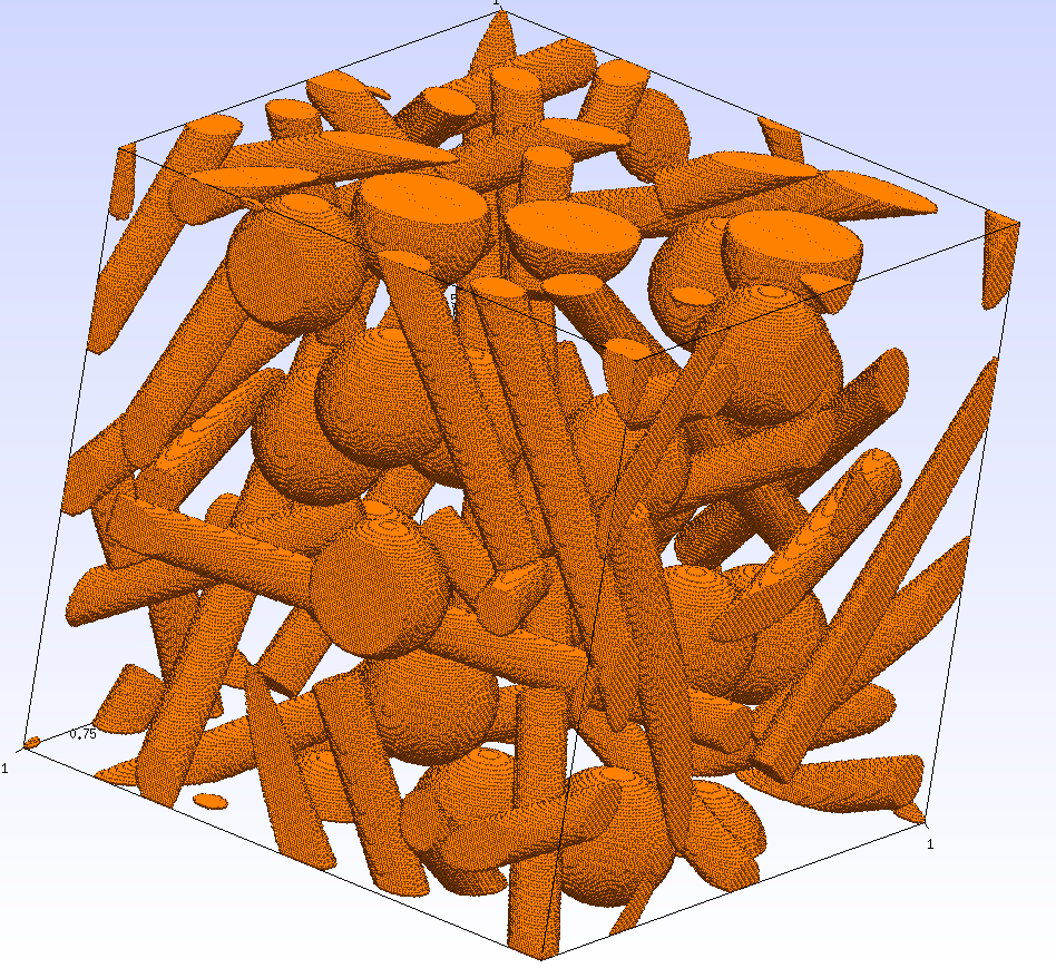
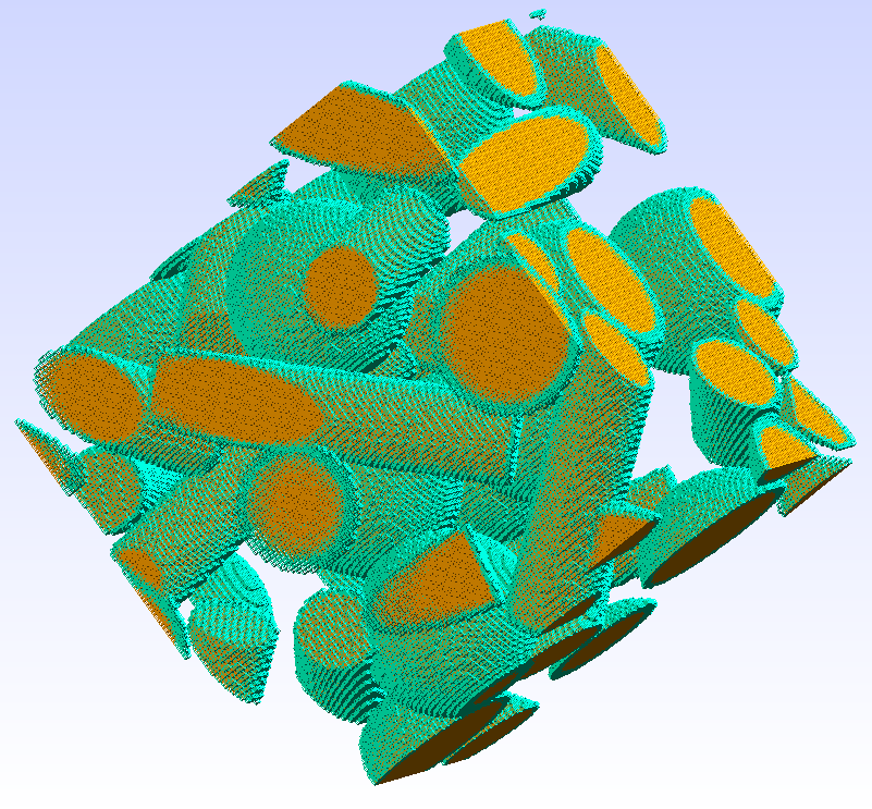
Though perfectly suitable for computations of elastic properties and in some cases of thermal ones, the generation procedure we have just described, clearly does not reflect the way how materials with good electrical conductivity are produced: the inclusions there should overlap or at least have some contacts to ensure continuity in the electric network they form. To cure this we use a simple trick to “puff up” the inclusions, i.e. increase their linear sizes, figure 1.(b). This does not spoil any isotropy, but creates eventual contacts and overlaps. The result is then a network of inclusions with eventual pairwise overlaps. The fact that this depicts rather well the real conducting composite materials used in industry may sound surprising, but actually it should not, since we are more or less modelling the actual process of their production. The first step of generating non-intersecting inclusions corresponds to placing them into the matrix, while “puffing up” in a simplified way mimics various external forces applied to the samples to ensure contacts. This qualitative logic is in some sense inspired by GSS , where some analysis of differential equations related to molecular dynamics is performed.
III Homogenization for electrical conductivity
After applying the method discussed in the previous section, we have a series of samples for each set of macroscopic parameters, let us now turn to the procedure for computing the effective electrical conductivity of those.
Certainly the best approach would be to honestly consider the Maxwell’s equations:
where is the electric flux, – charge density, – magnetic flux, – electric field, – magnetic field, – electric current density. One should consider these equations with different boundary conditions in order to recover the whole conductivity tensor. It is convenient to rewrite the equations only in terms of fields and not fluxes, using that , , with – permittivity of the material, its permiability; and (Ohm’s law) with – the conductivity. This gives:
Like this one sees the dependence on parameters coming from the medium, like and . And in our case these parameters do depend on spatial coordinates, since they are different for all the phases of the material.
In fact the problem can be significantly simplified since we are interested in a quasistationary regime without any charges inside the medium. Half of the equations thus become trivial, while the other half reduces precisely to the Fourier’s law in thermodynamics, with the temperature being the analogue of the electric potential, the heat flux – of the current, and – the conductivity tensor:
| (1) |
This permits also not to worry about well-posedness of the problem. One is thus tempted to apply the same FFT-based methods or use Finite Elements, as in the studies of thermal properties. Unfortunately, both approaches present serious difficulties. It has been observed in the original papers that the FFT-based methods are very sensitive to the contrast (ratio of conductivity) between the matrix and the inclusions, which is very high in the electric case – this results in a drastically slow convergence of the method. As for the FEM, the problem comes simply from the size of the mesh needed to capture microscopic geometry. We are thus brought to the need of a different method that we describe below.
Description of the method
The key idea is to study the structure of the network of inclusions that we have obtained in the previous section: consider the inclusions as nodes of an electric circuit, and say that those couples that have an overlap are connected. One thus obtains a connectivity graph of a sample with vertexes corresponding to inclusions and edges to contacts. Morally this means that we consider the inclusions made of a conducting material and the matrix is a perfect insulator. Already with this approach one can say something about conductivity and even more, see for example Luck , where networks of randomly distributed resistors are studied. But the information about connectivity is certainly not enough: we would like not only to say if the sample is conducting current or not, but also give a numerical estimate of this conductivity. It means that we should assign some resistance to each edge of the constructed graph. With this information we can then apply the Kirchhoff’s laws: for any internal vertex the sum of currents vanishes, and for any edge the classical Ohm’s law holds. The result will be the total current passing through the circuit – after some renormalization it gives precisely the desired conductivity. This idea is used very often for modelling complex systems, like traffic flow (book ), and it is simple enough to be very efficient. Paradoxically, we use Kirchhoff’s laws to actually compute the current, so “sometimes an electric circuit is just… an electric circuit”…
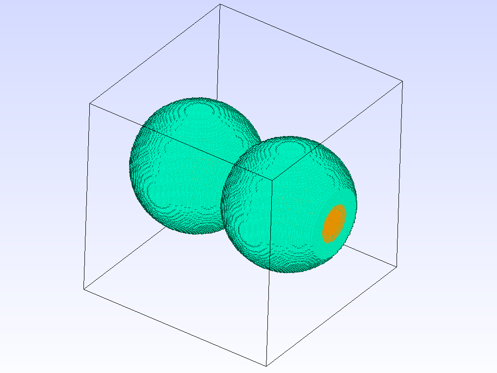
A crucial detail which remains to be discussed, is how to assign the values of resistance to edges – and this is a very important question, since complex geometry is taken into account precisely here. We profit again from the MD-based method of generating the samples described in VDP , namely from the table 1 there, which gives the expressions for repulsive forces between overlapping inclusions that depend on the geometry of overlaps. These forces, being rescaled appropriately, will characterize the resistance of the respective edge. By construction, these forces have elastic nature, so they give a good approximation of the law defining the resistance. By rescaling we mean selection of the constant factors in the formulas, since in the original setting they corresponded to mechanical forces and now we suppose the conductance (i.e. the inverse of resistance) to be proportional to those. For the law we consider, one just needs to fix the global normalization for each type of contacts. This is done by comparing the MD forces with the actual conductivity of the sample computed by FEM from Maxwell’s equations, which is doable for simple geometries. As one can see from figure 2, there are essentially three interesting types of overlaps: sphere-sphere, sphere-cylinder and cylinder-cylinder. For all of them small samples containing only a couple of inclusions are considered – those can be pixelized/meshed at some reasonably small resolution and thus are suitable for FEM. This step might be time consuming, but it is done only once to calibrate the model. On the other hand, one computes their conductivity using the electric circuit approach: the circuit would then contain just a couple of nodes, where one would adjust the constants to fit the FEM computation. Let us stress that this step is important, since it guarantees good agreement with the FEM that is often considered to be the second (after experimental tests) reliability criterion.
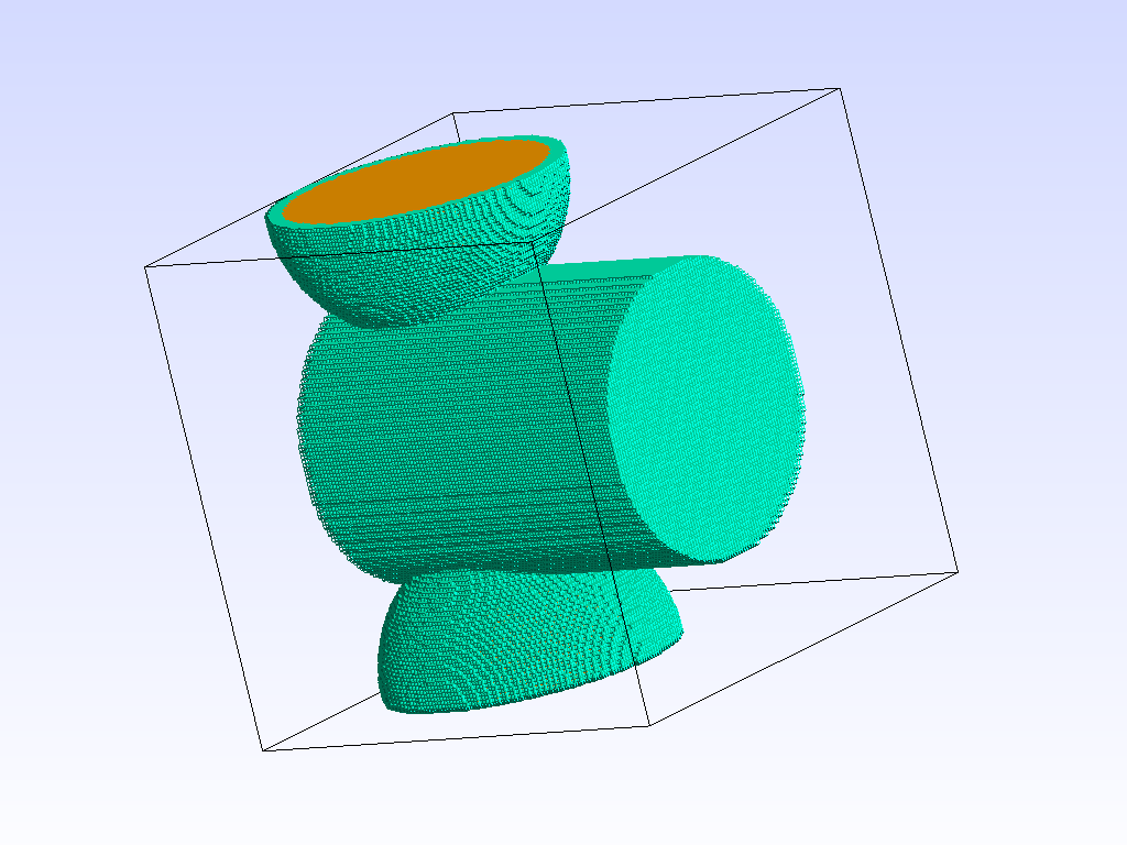
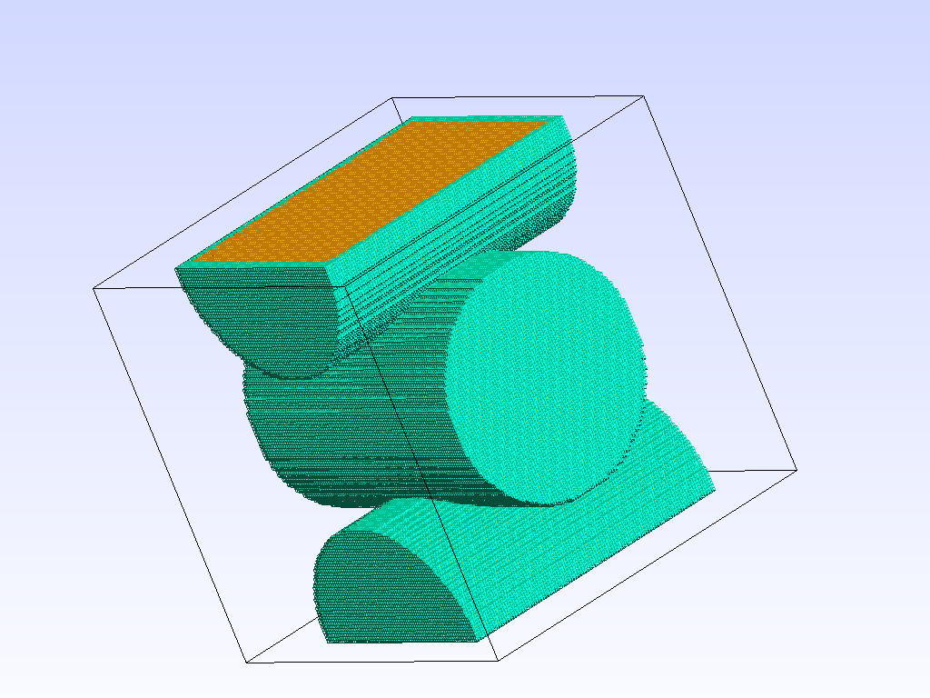
Certainly, one can consider more involved ways to model the interaction, for instance consider some non-linear dependence between the conductance and the MD force. One then would need to approximate that dependence by some function which will be reconstructed from the simple geometry pairwise overlaps. And again, that would be a potentially time consuming step, but done only once, thus this will not change the global strategy.
Homogenization example
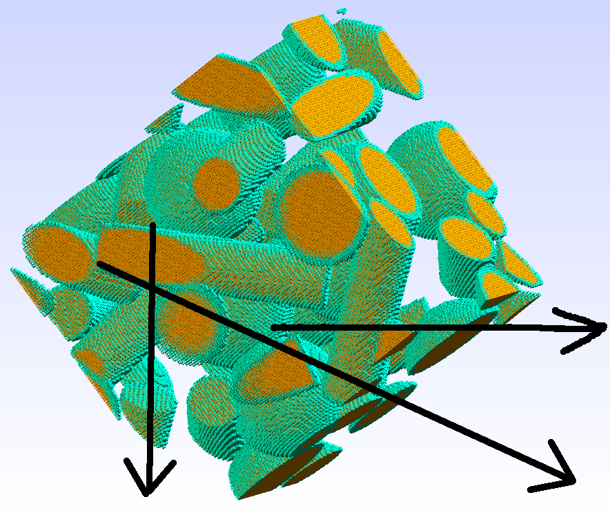
Let us consider a simple example – a sample with a small number of inclusions (figure 3 – left). It is of course out of the VER notion, we present it only to illustrate the computation procedure. One can see clearly that this sample is percolating, i.e. there is a path of inclusions connecting two boundaries, so even with a small volume fraction of inclusions it does conduct current.
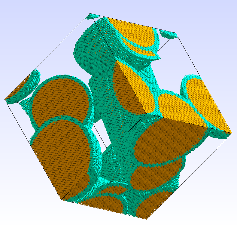

Let us now construct the corresponding graph (figure 3 – right ) and its adjacency matrix. As described above all the inclusions are represented by vertexes: 3 for spheres and 3 for cylinders, we denote them () and () respectively. We add to them two vertexes that correspond to boundaries: and . If an inclusion touches the boundary or another inclusion we draw an edge between the corresponding vertexes and assign a weight to it equal to the conductance computed from the MD procedure described above. The (weighted) adjacency matrix is constructed by putting the values on the intersection of lines and columns corresponding to the vertexes that define the edge , then the resulting matrix has the following form:
This corresponds to the ordering of vertexes: , and the delimited upper-left and lower-right corners represent the opposite boundaries and . The matrix is symmetric, and only off-diagonal values are important. The boxed non-zero numbers come from the construction described above, there are precisely of them, since there are non-trivial contacts, and if one looks only at the upper triangle they are ordered line by line in the same way as ’s.
In principal this data would be already enough to solve the problem, but in order to make the implementation more transparent let us introduce one more graph-related object – the incidence matrix . The lines of it are indexed by the vertexes of the graph and the columns by the edges. The entries are if the edge comes out or goes into a given vertex, and otherwise. In our example for the same ordering of vertexes as before it reads:
This matrix can be read off from or constructed directly, provided the number of edges is known. If one considers the vector , then the weighted degree matrix can be constructed, as well as the conductance matrix . One then recovers the adjacency matrix .
But the most important application of is not the identity above. Actually, it carries the information about the structure of the linear system that will be used to compute the effective conductivity of the sample. Let us enumerate the unknowns, which split into two types: the values of the electric potential at each vertex ( of them here, denoted ), and the current through each edge ( of them, denoted ). One easily notices that the columns of correspond to currents, namely they encode the Ohm’s law for each edge: , where the indexes for are precisely the lines with non-zero entries for the -th column; this gives 13 linear conditions. The lines (all but the first and the last ones) correspond to the Kirchhoff’s law for the internal nodes: ; this gives 6 more linear conditions. And we impose some values of potential on the boundary, say and , which complete the linear system. Clearly this counting of unknowns and equations remains valid for any graph. Then it is enough to solve the obtained system, or better to say compute the total current through the circuit, to obtain the effective resistance of the sample in the direction between the two boundaries. Here again the structure of the matrix is helpful: this total current is the sum of outgoing currents from the first boundary (indexed in the first line of ) or of incoming currents to the second boundary (the last line of respectively). In this concrete example the computed value is approximately .
This is the scheme of the homogenization procedure we suggest. To complete the picture, one needs to perform similar computations for all the couples of boundaries of the domain to recover the whole conductivity tensor from the equation (1). The opposite faces of the cube will correspond to diagonal and the neighboring to off-diagonal entries. For these latter ones it is important to treat adequately the inclusions that are in contact with both faces: a possible reasonable choice is to consider only the central part of the boundary, or even just the central point.
A couple of technical remarks are in place here. First, we have reduced the homogenization problem to solving a linear system. It may be rather large for “by hand” solution, but it is very small if one compares with those that arise in for example Finite Elements. This means that basically any available solver would do the job, one just need to pay attention to possible degeneracies. We mean the following: the system is never overdetermined and it is consistent by construction, but it can be degenerate. This is easy to understand from the physics of the problem: the graph we construct from the network of inclusions need not be connected (imagine an isolated inclusion inside the matrix) then to the parts not connected to boundaries one can assign any value of the electric potential. But this is the only freedom in the solution, so the result of the homogenization procedure is well defined. Second, in contrast to our toy example, already the adjacency matrix in the typical situation is rather sparse, and this is even more pronounced for the final linear system. One can thus profit from this knowledge to choose appropriate solvers and optimize even more the computation time. Alternatively, one can remember that the system was coming from graphs, and profit from various packages available for their analysis.
IV Test examples, applications, and discussion
Let us now put the procedures described in the previous sections together and see what happens
in real stochastic homogenization computations.
IV.1 Test examples
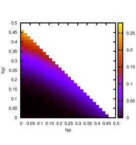
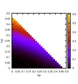
We consider the samples containing a mixture of spherical and cylindrical inclusions, and study the dependence of their electrical conductivity on the volume fraction of each type of inclusions. Below (figure 4) we plot this value for two types of tests, for different aspect ratios (length/radius) of cylinders, the value is averaged over a series of samples with the same macroscopic parameters, but different microgeometry. The output is given in dimensionless units, where the value of corresponds to maximal conductivity, i.e. the sample made of pure conducting material, or equivalently the volume fraction of inclusions being . One sees that for longer cylinders the conductivity of samples increases in the average. Certainly this is rather a consistency test for the method we suggest than a real systematic study of the effects of morphology of inclusions on the effective properties of materials, that we intend to do in a separate article. The main message of this paper is precisely that using rather simple and accessible tools and computations that run in fractions of a second, one can already obtain convincing results.
IV.2 Industrial applications
As we have already mentioned, behind this study there is a concrete applied problem related to estimation and improvement of effective properties of composite materials. In real-life applications one does not work with precisely the same samples that we have discussed in section II, they do look like figure 1, but have a completely different origin. Usually one obtains this picture not by pixelizing the vector data of the set of inclusions, but the other way around – for example from tomography or microscopy. Then image processing algorithms are used to segment the image, i.e. distinguish the material that is represented by each voxel. Even though modern algorithms permit to make this distinction if a given voxel belongs to the matrix or to inclusions with rather good certainty, the information to which inclusion precisely it belongs is not available directly.
But we are still able to handle the situation with our approach. In a sense, the geometric part is even
simpler in this case: one considers voxels corresponding to inclusions
as independent particles, and the connectivity graph is just the information about neighbouring voxels.
As for the forces assigned to edges, now one needs to consider three cases of voxels that meet by a face, by an edge or by a vertex,
and adjust the constants appropriately.
The price one pays is certainly the size of the resulting linear system,
so the observation about sparsity becomes extremely important.
This looks like a “baby version” of Finite Elements, but it is still
much simpler both from mathematical and from algorithmic points of view.
Moreover, the computation being local, the algorithm should be suitable for parallelization.
IV.3 Discussion
We have described a procedure permitting to compute effective electric properties of composite materials using very efficient and accessible tools. Since the required computational resources are very modest it is appropriate for stochastic homogenization. This provides a tool both for analytical studies and industrial applications. However there is a couple of questions we are curios about and intend to address them in the nearest future. First, as mentioned before, the test problems and some research ones do not need huge computational resources, while industrial applications eventually do. In what we have discussed above, the solution of the linear system was (theoretically) exact, but in real life this might be not needed. We think that the link with graphs in the context is very promising and can provide efficient and reliable ways to handle the problem. Second, by construction our method is in good agreement with FEM, since the latter one is implicitly used. It means that at least for simple geometry of samples, the obtained solutions reproduce well the ones obtained from Maxwell’s equations. It would be interesting to observe and eventually prove the same thing for the FFT-based methods.
Acknowledgements.
This work has been supported by the ACCEA project selected by the “Fonds Unique Interministériel (FUI) 15 (18/03/2013)” program. The research of V.S. was also supported by the Fonds National de la Recherche, Luxembourg, project F1R-MTH-AFR-080000.
References
- (1) J.C. Michel, H. Moulinec and P. Suquet, A computational scheme for linear and non-linear composites with arbitrary phase contrast, Int. J. Numer. Meth. Engng 2001; 52:139–160 (DOI: 10.1002/nme.275).
- (2) V. Monchiet, and G. Bonnet, A polarization-based FFT iterative scheme for computing the effective properties of elastic composites with arbitrary contrast, Int. J. Numer. Meth. Engng (2011).
- (3) V. Salnikov, S. Lemaitre, D. Choï, P. Karamian-Surville, Measure of combined effects of morphological parameters of inclusions within composite materials via stochastic homogenization to determine effective mechanical properties. Composite Structures, Vol. 129, 2015.
- (4) S. Lemaitre, V. Salnikov, D. Choi, P. Karamian, Computation of thermal properties via 3D homogenization of multiphase materials using FFT-based accelerated scheme. Preprint: arXiv:1504.07499
- (5) S. Lemaitre, V. Salnikov, D. Choi, P. Karamian, Influence of morphological parameters in 3D composite materials on their effective thermal properties and comparison with effective mechanical properties, Preprint: arXiv:1602.07851
- (6) S. Lemaitre, V. Salnikov, D. Choi, P. Karamian, Adapting FFT-based computational schemes to analysis of thermal and electrical conductivity of composite materials: cases of high contrast, in preparation.
- (7) V. Salnikov, D. Choi, P. Karamian, On efficient and reliable stochastic generation of RVEs for analysis of composites within the framework of homogenization, Comput. Mechanics, 55, 2015.
- (8) S. Lemaitre, V. Salnikov, D. Choi, P. Karamian, Génération de VER 3D par la dynamique moléculaire et variations autour de la pixellisation. Calcul des propriétés effectives des composites, proceedings of CSMA 2015.
- (9) B. Widom, Random Sequential Addition of Hard Spheres to a Volume, J. Chem. Phys. 44, 3888 (1966).
- (10) B. D. Lubachevsky, F.H. Stillinger, Geometric properties of random disk packings Journal of Statistical Physics, 08/1990; 60(5):561-583.
- (11) T. Kanit, S. Forest, I. Galliet, V.Mounoury, D.Jeulin, Determination of the size of the representative volume element for random composites: statistical and numerical approach. Int. J. Solids Struct, 40:3647–3679, 2003.
- (12) V. L. Golo, Vl. N. Salnikov, and K. V. Shaitan, Harmonic Oscillators in the Nosé-Hoover Environment, Physical Review, E70, 046130, 2004.
- (13) J. M. Luck, Conductivity of random resistor networks: An investigation of the accuracy of the effective-medium approximation, Physical Review B, 43, 5, 1991.
- (14) G. Grimmett, Probability on Graphs, Cambridge University Press, 2011.