22institutetext: Toyota Motors North America R&D, 22email:
Logical Clustering and Learning
for Time-Series Data
Abstract
In order to effectively analyze and build cyberphysical systems (CPS), designers today have to combat the data deluge problem, i.e., the burden of processing intractably large amounts of data produced by complex models and experiments. In this work, we utilize monotonic parametric signal temporal logic (PSTL) to design features for unsupervised classification of time series data. This enables using off-the-shelf machine learning tools to automatically cluster similar traces with respect to a given PSTL formula. We demonstrate how this technique produces interpretable formulas that are amenable to analysis and understanding using a few representative examples. We illustrate this with case studies related to automotive engine testing, highway traffic analysis, and auto-grading massively open online courses.
1 Introduction
In order to effectively construct and analyze cyber-physical systems (CPS), designers today have to combat the data deluge problem, i. e., the burden of processing intractably large amounts of data produced by complex models and experiments. For example, consider the typical design process for an advanced CPS such as a self-driving car. Checking whether the car meets all its requirements is typically done by either physically driving the car around for millions of miles [2], or by performing virtual simulations of the self-driving algorithms. Either approach can generate several gigabytes worth of time-series traces of data, such as sensor readings, variables within the software controllers, actuator actions, driver inputs, and environmental conditions. Typically, designers are interested not in the details of these traces, but in discovering higher-level insight from them; however, given the volume of data, a high level of automation is needed.
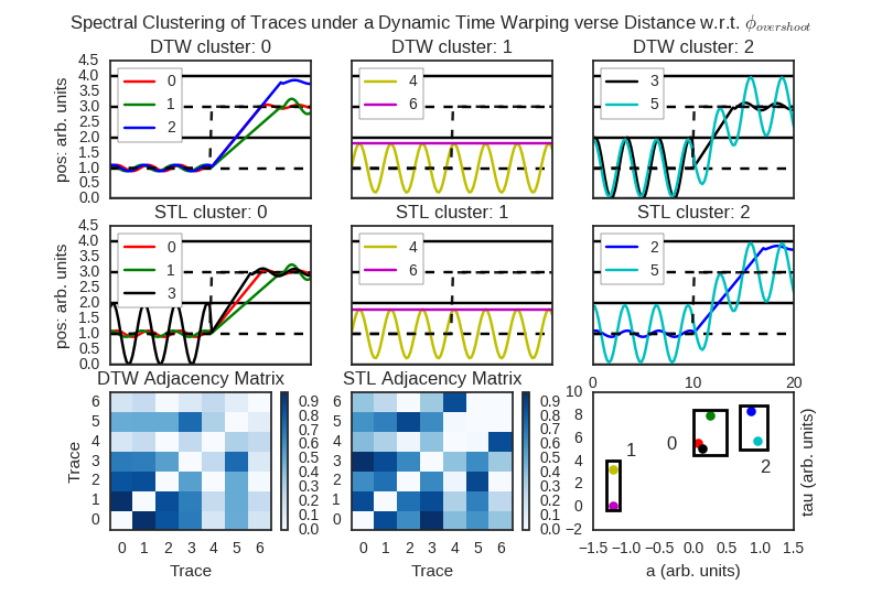
The key challenge then is: “How do we automatically identify logical structure or relations within such data?” One possibility offered by unsupervised learning algorithms from the machine learning community is to cluster similar behaviors to identify higher-level commonalities in the data. Typical clustering algorithms define similarity measures on signal spaces, e. g., the dynamic time warping distance, or by projecting data to complex feature spaces. We argue later in this section that these methods can be inadequate to learn logical structure in time-series data.
In this paper, we present logical clustering, an unsupervised learning procedure that utilizes Parametric Signal Temporal Logic (PSTL) templates to discover logical structure within the given data. Informally, Signal Temporal Logic (STL) enables specifying temporal relations between constraints on signal values [10, 3]. PSTL generalizes STL formulas by replacing, with parameters, time constants in temporal operators and signal-value constants in atomic predicates in the formula. With PSTL templates, one can use the template parameters as features. This is done by projecting a trace to parameter valuations that correspond to a formula that is marginally satisfied by the trace. As each trace is projected to the finite-dimensional space of formula-parameters, we can then use traditional clustering algorithms on this space; thereby grouping traces that satisfy the same (or similar) formulas together. Such logical clustering can reveal heretofore undiscovered structure in the traces, albeit through the lens of an user-provided template. We illustrate the basic steps in our technique with an example.
Consider the design of a lane-tracking controller for a car and a scenario where a car has effected a lane-change. A typical control designer tests design performance by observing the “overshoot” behavior of the controller, i. e., by inspecting the maximum deviation (say ) over a certain duration of time (say, ) of the vehicle position trajectory from a given desired trajectory . We can use the following PSTL template that captures such an overshoot:
| (1) |
When we project traces appearing in Fig. 1 through , we find three behavior-clusters as shown in the second row of the figure: (1) Cluster 0 with traces that track the desired trajectory with small overshoot, (2) Cluster 1 with traces that fail to track the desired trajectory altogether, and (3) Cluster 2 with traces that do track the desired trajectory, but have a large overshoot value. The three clusters indicate a well-behaved controller, an incorrect controller, and a controller that needs tuning respectively. The key observation here is that though we use a single overshoot template to analyze the data, qualitatively different behaviors form separate clusters in the induced parameter space; furthermore, each cluster has higher-level meaning that the designer can find valuable.
In contrast to our proposed method, consider the clustering induced by using the dynamic time warping (DTW) distance measure as shown in Fig. 1. Note that DTW is one of the most popular measures to cluster time-series data [17]. We can see that traces with both high and low overshoots are clustered together due to similarities in their shape. Such shape-similarity based grouping could be quite valuable in certain contexts; however, it is inadequate when the designer is interested in temporal properties that may group traces of dissimilar shapes.
In Section 3, we show how we can use feature extraction with PSTL templates to group traces with similar logical properties together. An advantage of using PSTL is that the enhanced feature extraction is computationally efficient for the fragment of monotonic PSTL formulas [5, 14]; such a formula has the property that its satisfaction by a given trace is monotonic in its parameter values. The efficiency in feature extraction relies on a multi-dimensional binary search procedure [20] that exploits the monotonicity property.
A different view of the technique presented here is as a method to perform temporal logic inference from data, such as the work on learning STL formulas in a supervised learning context[7, 18, 5, 6], in the unsupervised anomaly detection context[15], and in the context of active learning[16]. Some of these approaches adapt classical machine learning algorithms such as decision trees [7] and one-class support vector machines [15] to learn (possibly, arbitrarily long) formulas in a restricted fragment of STL. Formulas exceeding a certain length are often considered inscrutable by designers. A key technical contribution of this paper is to show that using simple shapes such as specific Boolean combinations of axis-aligned hyperboxes in the parameter space of monotonic PSTL to represent clusters yields a formula that may be easier to interpret. We support this in Section 4, by showing that such hyperbox-clusters correspond to STL formulas that have length linear in the number of parameters in the given PSTL template, and thus of bounded descriptive complexity.
Mining parametric temporal logic properties in a model-based design has also been explored [14, 12]. We note that our proposed methods does not require such a model, which may not be available either due to the complexity of the underlying system or lack of certainty in the dynamics. We also note that there is much work on mining discrete temporal logic specifications from data (e.g. [21]): our work instead focuses on unsupervised learning of STL properties relevant to CPS.
The reader might wonder how much insight is needed by a user to select the PSTL template to use for classification. We argue the templates do not pose a burden on the user and that our technique can have high value in several ways. First, we observe that we can combine our technique with a human-guided (or automated) enumerative learning procedure that can exploit high-level template pools. We demonstrate such a procedure in the diesel engine case study. Second, consider a scenario where a designer has insight into the data that allows them to choose the correct PSTL template. Even in this case, our method automates the task of labeleing trace-clusters with STL labels which can then be used to automatically classify new data. Finally, we argue that many unsupervised learning techniques on time-series data must “featurize” the data to start with, and such features represent relevant domain knowledge. Our features happen to be PSTL templates. As the lane controller motivating example illustrates, a common procedure that doesn’t have some domain specific knowledge increases the risk of wrong classifications. This sentiment is highlighted even in the data mining literature [22]. To illustrate the value of our technique, in Sec. 5, we demonstrate the use of logic-based templates to analyze time-series data in case studies from three different application domains.
2 Preliminaries
Definition 1 (Timed Traces)
A timed trace is a finite (or infinite) sequence of pairs , , , where, , and for all , , , and for , , where is some compact set. We refer to the interval as the time domain .
Real-time temporal logics are a formalism for reasoning about finite or infinite timed traces. Logics such as the Timed Propositional Temporal Logic [4], and Metric Temporal Logic (MTL) [19] were introduced to reason about signals representing Boolean-predicates varying over dense (or discrete) time. More recently, Signal Temporal Logic [23] was proposed in the context of analog and mixed-signal circuits as a specification language for real-valued signals.
Signal Temporal Logic. Without loss of generality, atoms in STL formulas can be be reduced to the form , where is a function from to , , and . Temporal formulas are formed using temporal operators, “always” (denoted as ), “eventually” (denoted as ) and “until” (denoted as ) that can each be indexed by an interval . An STL formula is written using the following grammar:
| (2) |
In the above grammar, , and . The always () and eventually () operators are defined for notational convenience, and are just special cases of the until operator: , and . We use the notation to mean that the suffix of the timed trace beginning at time satisfies the formula . The formal semantics of an STL formula are defined recursively:
We write as a shorthand of .
Parametric Signal Temporal Logic (PSTL). PSTL [5] is an extension of STL introduced to define template formulas containing unknown parameters. Formally, the set of parameters is a set consisting of two disjoint sets of variables and of which at least one is nonempty. The parameter variables in can take values from their domain, denoted as the set . The parameter variables in are time-parameters that take values from the time domain . We define a valuation function that maps a parameter to a value in its domain. We denote a vector of parameter variables by , and extend the definition of the valuation function to map parameter vectors into tuples of respective values over or . We define the parameter space as a subset of .
A PSTL formula is then defined by modifying the grammar specified in (2) by allowing to be elements of , and to be an element of . An STL formula is obtained by pairing a PSTL formula with a valuation function that assigns a value to each parameter variable. For example, consider the PSTL formula = , with parameters variables and . The STL formula is an instance of obtained with the valuation .
Monotonic PSTL. Monotonic PSTL is a fragment of PSTL introduced as the polarity fragment in [5]. A PSTL formula is said to be monotonically increasing in parameter if condition (3) holds for all , and is said to be monotonically decreasing in parameter if condition (4) holds for all .
| (3) | |||||
| (4) |
To indicate the direction of monotonicity, we now introduce the polarity of a parameter[5], , and say that if the is monotonically increasing in and if it is monotonically decreasing, and if it is neither. A formula is said to be monotonic in if , and say that is monotonic if for all , is monotonic in .
While restrictive, the monotonic fragment of PSTL contains many formulas of interest, such as those expressing steps and spikes in trace values, timed-causal relations between traces, and so on. Moreover, in some instances, for a given non-monotonic PSTL formula, it may be possible to obtain a related monotonic PSTL formula by using distinct parameters in place of a repeated parameter, or by assigning a constant valuation for some parameters (Example in Sec 6).
Example 1
For formula (1), we can see that , because if a trace has a certain overshoot exceeding the threshold , then for a fixed , the trace satisfies any formula where . Similarly, = , as an overshoot over some interval will be still considered an overshoot for .
Orders on Parameter Space. A monotonic parameter induces a total order in its domain, and as different parameters for a given formula are usually independent, valuations for different parameters induce a partial order:
Definition 2 (Parameter Space Partial Order)
We define as a total order on the domain of the parameter as follows:
| (5) |
Under the order , the parameter space can be viewed as a partially ordered set , where the ordering operation is defined as follows:
| (6) |
When combined with eqs (3), (4) this gives us the relation that implies that . In order to simplify notation, we define the subset of that satisfies as . If and are obvious from context, we simply write: . It follows that . In summary: operates in the same direction as implication and subset. Informally, we say that the ordering is from a stronger to a weaker formula.
Example 2
For formula (1), the order operation is defined as iff and . Consider and . As , , , and . Intuitively this means that if satisfies a formula specifying a overshoot (undershoot ) over a duration of time units, then trivially satisfies the formula specifying an undershoot of over a duration of time units.
Next, we define the downward closure of and relate it to .
Definition 3 (Downward closure of a valuation)
For a valuation , its downward closure (denoted ) is the set .
In the following lemma we state that the union of the sets of traces satisfying formulas corresponding to parameter valuations in the downward closure of a valuation is the same as the set of traces satisfying the formula corresponding to . The proof follows from the definition of downward closure.
Lemma 1
Lastly, we define the validity domain of a set of traces and .
Definition 4 (Validity domain)
Let be a (potentially infinite) collection of timed traces, and let be a PSTL formula with parameters . The validity domain111If is obvious from context (or does not matter), we write as . of is a closed subset of , such that:
| (7) |
Remark 1
The validity domain for a given parameter set essentially contains all the parameter valuations s.t. for the given set of traces , each trace satisfies the STL formula obtained by instantiating the given PSTL formula with the parameter valuation.
Example 3
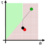
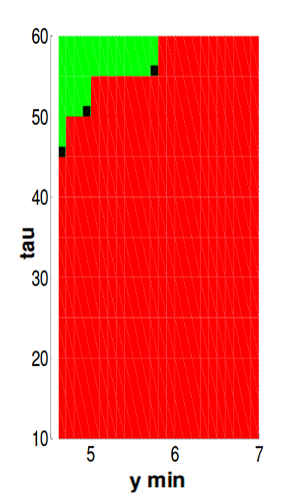
In Fig. 2, we show the validity domain of the PSTL formula (1) for the three traces given in the subplot labeled STL cluster 0 in Fig. 1. The hatched red region contains parameter valuations corresponding to STL formulas that are not satisfied by any trace, while the shaded-green region is the validity domain of the formula. The validity domain reflects that till the peak value of the black trace is reached (which is the smallest among the peak values for the three signals), the curve in - space follows the green trace (which has the lowest slope among the three traces). For any value of , for which , the formula is trivially satisfied by all traces.
3 Trace-Projection and Clustering
In this section, we introduce the projection of a trace to the parameter space of a given PSTL formula, and discuss mechanisms to cluster the trace-projections using off-the-shelf clustering techniques.
Trace Projection. The key idea of this paper is defining a projection operation that maps a given timed trace to a suitable parameter valuation222For canonicity, need not be a function from timed traces to . For example, it may be expedient to project a trace to a subset of . For simplicity, we defer more involved projections to future exposition. in the validity domain of the given PSTL formula . We would also like to project the given timed trace to a valuation that is as close a representative of the given trace as possible (under the lens of the chosen PSTL formula).
One way of mapping a given timed trace to a single valuation is by defining a total order on the parameter space by an appropriate linearization of the partial order on parameter space. The total order then provides a minimum valuation to which the given timed trace is mapped.
Remark 2
For technical reasons, we often adjoin two special elements and to such that , and , and . These special elements mark whether is the whole parameter space or empty.
We present the lexicographic order on parameters as one possible linearization; other linearizations, such as those based on a weighted sum in the parameter space could also be used (presented in Sec 6 for brevity).
Lexicographic Order. A lexicographic order (denoted ) uses the specification of a total order on parameter indices to linearize the partial order. We formalize lexicographic ordering as follows.
Definition 5 (Lexicographic Order)
Suppose we are given a total order on the parameters . The total order on the parameter space is defined as:
| (8) |
Note that for a given total or partial order, we can define and under that order in standard fashion. Formally, the projection function using lexicographic order is defined as follows:
| (9) |
Computing . To approximate , we recall Algorithm 1 from [14] that uses a simple lexicographic binary search333For simplicity, we have omitted a number of optimizations in Algorithm 1. For example, one can replace the iterative loop through parameters with a binary search over parameters..
We begin by setting the interval to search for a valuation in . We set the initial valuation to since it induces the most permissive STL formula. Next, for each parameter, (in the order imposed by ), we perform bisection search on the interval to find a valuation in . Once completed, we return the lower bound of the search-interval as it is guaranteed to be satisfiable (if a satisfiable assignment exists).
Crucially, this algorithm exploits the monotonicity of the PSTL formula to guarantee that there is at most one point during the bisection search where the satisfaction of can change. The number of iterations for each parameter index is bounded above by , and the number of parameters. This gives us an algorithm with complexity that grows linearly in the number of parameters and logarithmically in the desired precision.
Remark 3
Pragmatically, we remark that the projection algorithm is inherently very parallel at the trace level and as such scales well across machines.
Example 4
For the running example (PSTL formula (1)), we use the order . As , and , lexicographic projection has the effect of first searching for the largest , and then searching for the smallest such that the resulting valuation is in . The projections of the three traces from STL cluster 0 from Fig. 1 are shown in Fig. 2. We use the same color to denote a trace and its projection in parameter space.
Clustering and Labeling.
What does one gain by defining a projection, ? We posit that applying unsupervised learning algorithms for clustering in lets us glean insights about the logical structure of the trace-space by grouping traces that satisfy similar formulas together. Let be a finite, nonempty set of labels. Let represent a user-provided set of traces. In essence, a clustering algorithm identifies a labeling function assigning to each trace in zero or more labels. We elaborate with the help of an example.
Example 5
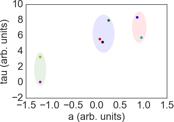
In Fig. 3, we show a possible clustering induced by using Gaussian Mixture Models444A GMM assumes that the given parameter space can be modeled as a random variable distributed according to a set of Gaussian distributions with different mean and variance values. A given parameter valuation is labeled if the probability of the valuation belonging to the Gaussian distribution exceeds the probability of the valuation belonging to other distributions. Another way to visualize clusters in the parameter space is by level-sets of the probability density functions associated with the clusters. For example, for the cluster, we can represent it using the smallest level-set that includes all given points labeled . (GMMs) for the trace-projections for the traces in Fig. 1. The figure shows that the traces colored green, red and black are grouped in the same cluster; this matches the observation that all three traces have behaviors indicating overshoots, but of reasonable magnitudes. On the other hand, traces colored magenta and yellow have no overshoot and are grouped into a second cluster. The final cluster contains the blue and cyan traces, both with a large overshoot.
Supposing the clustering algorithm reasonably groups traces satisfying similar parameter valuations/logical formulas, one may ask: “Can we describe this group of traces in terms of an easily interpretable STL formula?” Using an ellipsoid to represent a cluster, unfortunately, the answer is negative.
Example 6
It is clear that formula (10) is inscrutable, and actually represents an infinite number of STL formulas. In case of GMMs, we can at least have an abstract description of clusters using ellipsoid shapes in the parameter-space. If we use spectral clustering (as described in Section 1), the representation of a cluster in the parameter space is even less obvious. To mitigate this problem, we observe that the distance between points in is a “good” proxy for whether they receive the same label. Thus, another way to define the labeling function , is via parameter ranges. We argue that the use of axis-aligned hyperboxes enclosing points with the same labels is a useful approximation of the clusters, particularly because as we see in the next section, it has a compact STL encoding.
Remark 4
For a given set of points, the tightest-enclosing hyperbox may include points that would not have received the same label by an off-the-shelf clustering algorithm. This can lead to a scenario where hyperbox-clusters intersect (see Fig. 5c in for an example). This means that we can now have points in the parameter space that can have possibly two or more labels. We argue that this can be addressed in two ways: (1) introduce a new hyperbox cluster for points in the intersection, (2) indicate that points in the intersection represent traces for which there is additional guidance required from the designer.
Hyperbox Clusters. In the previous section, we showed that we can construct a labeling function to assign labels to the user-provided set of traces . We now see how we can extend this labeling function to all possible traces .
Let . A valid hyperbox in the parameter space is defined in terms of its extreme points , (where ), where and are the infimum and supremum resp. over the box w.r.t. . Formally,
Definition 6 (Hyperbox)
| (11) |
In other words, we assume that a hyperbox is open on all faces not connected to the infimum of the box, unless the face is connected to the supremum of . Let denote the set of all such hyperboxes.
Definition 7 (Hyperbox Labeling Function)
Given a trace and a hyperbox , s.t. , we define as the hyperbox labeling function from to as follows:
| (12) |
In other words, we only consider hyperboxes that contain the projections of all traces with a specific label (say ), and then any trace that projects to some point in the hyperbox gets all such labels . We extend the definition to boxes, such that . We note that represents the smallest set containing all parameter valuations that are labeled . However, does not satisfy the definition of a hyperbox as per Definition 6 as it is a closed set. Hence, we define an relaxation of this set as the smallest bounding hyperbox satisfying Definition 6 at Hausdorff distance from , and call it the -bounding hyperbox. In the next section, we show how we can translate a cluster represented as an -bounding hyperbox to an STL formula. We will further examine how, in some cases, we can represent a cluster by a superset of the -bounding hyperbox that satisfies , but allows a simpler STL representation.
Example 7
For the example shown in Fig. 1, for each of the red, green and black traces , , while for the blue and cyan traces, . Any hyperbox satisfying Definition 6 that is a superset of the hyperbox enclosing the red, green and black points shown in the bottom right figure has , while the hyperbox shown in the figure is an -bounding hyperbox.
4 Learning STL Formulas from Clusters
A given -bounding hyperbox simply specifies a range of valuations for the parameters in a PSTL template . We now demonstrate that because is monotonic, there exists a simple STL formula that is satisfied by the set of traces that project to some valuation in . Recall that we use to denote the set of traces that satisfies . We define as the set of traces that have a satisfying valuation in :
Theorem 4.1
There is an STL formula such that .
Before proving this theorem, we introduce some notation:
Definition 8 (Essential Corners, )
Let , and let . A valuation corresponding to an essential corner has exactly one such that , and for all , .
Proof (Theorem 4.1)
We first introduce the notion of essential corners of a box .
Note that can be written in terms of downward closures of valuations: . From Lemma 1, the set of traces satisfying a formula in is equivalent to . Further, using the equivalence between intersections () of sets of traces and conjunctions () in STL, and equivalence of set-complements with negations, we define below and note that the set of traces satisfying the formula below is .
| (13) |
Example 8
Consider the enclosing the projections for the yellow and magenta traces (Cluster 1). The corner-points of the cluster in clockwise order from bottom right corner are: , , , . Observe that as and , = , = . Thus, = . Thus:
| (14) |
Lemma 2
Proof
Recall from Def 8 that corners in have exactly 1 param set to . There are params, thus by pigeon hole principle, . In for each corner in , the corresponding formula is negated, adding 1 symbol. Between each instantiations of is a . Thus
Simplifying STL representation. To motivate this section, let us re-examine Example 8. From Fig. 1, we can observe that there is no hyperbox cluster to the left of or above the chosen hyperbox cluster , i. e., the one containing the magenta and yellow trace-projection. What if we consider supersets of that are hyperboxes and have the same infimum point? For Example 8, we can see that any hyperbox that extends to the supremum of the parameter space in or direction would be acceptable as an enclosure for the yellow and magenta traces (as there are no other traces in those directions). We formalize this intuition in terms of relaxing the set of corners that can appear in .
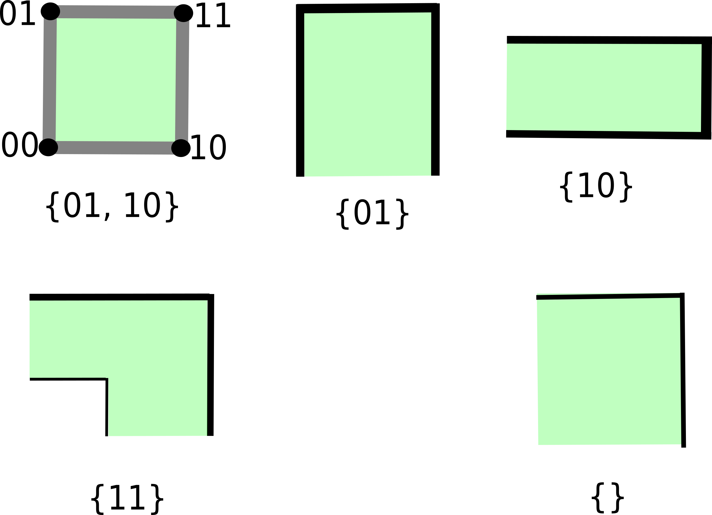
For instance, suppose that we replace in Eq (13) with , where is any subset of the corners of (excluding ). We call the collection of shapes induced by this relaxation as . For , the possible shapes of elements in are shown in Fig. 4. For convenience, we use a bit-vector encoding for hyperbox corners, where corresponds to the bit-vector with all s, has all s, and essential corners are bit-vectors with exactly one . Consider the L shaped region, , created by . The formula corresponding to has obviously less descriptive complexity than . Further notice, would have less descriptive complexity than elements of .
One critical feature that (and thus ) has is comparable convexity:
Definition 9 (Comparable Convexity)
If if or then all convex combinations of and are in .
Comparable convexity allows us to argue that one can gain some insight into the set of traces by just examining the extremal cases and just “interpolating” the cases because of the associated parameters. We call these extremal cases the “representatives” of a cluster.
Theorem 4.2
Each element in is comparably convex. See Fig. 4 for examples.
Proof
Note that all elements of are trivially comparably convex since hyperboxes are convex. Thus we focus on elements of . Now observe that any element is the union of a finite set, , of boxes in . s.t. where and . If or the other way around or or , then again there trivially the convex combination of and is in because hyperboxes are convex (and the intersection of two hyperboxes is a hyperbox).
This leaves the case where and and neither nor . This implies that is not comparable to . W.L.O.G assume and that the convex combination of and is not a subset . Note that the definition of downward closure and the fact that . But, is convex and , thus the convex combination of and is in which is a contradiction.
5 Case Studies
Implementation Details. We leveraged Breach [9] for performing projections , - toolkit [11] for clustering and custom Python code for learning STL formulas for clusters. An IPython notebook with compressed versions of the datasets studied in the case studies (and a replementation of in Python) is available for download at [1].
Diesel Engine. In this case study, we are provided with timed traces for a signal representing the Exhaust Gas Recirculation (EGR) rate for an early prototype of a Diesel Engine airpath controller. As the example comes from an automotive setting, we suppress actual signal values for proprietary reasons. The controller computes an EGR reference rate and attempts to track it. Typically, engineers visually inspect the step-response of the control system and look for patterns such as unusual overshoots, slow responsiveness, etc. The ST-Lib library [13] defines a pool of PSTL formulas designed to detect violations of such properties. Using a property from ST-Lib requires correctly setting the parameters in the PSTL templates therein. In this case study, we show how we can use our technique to determine parameters that characterize undesirable behavior. We focus on two templates: Rising Step and Overshoot. Many ST-Lib formulas are “step-triggered”, they are of the form: We first identify parameters for the step template, as it is used as a primitive in further analysis. For example, in the overshoot analysis we seek to characterize by what margin traces overshoot the reference. We use the following templates for rising-step and overshoot:
| (15) | ||||
| (16) |
Eq (15) first reduces step detection (via a discrete derivative) to spike detection and then applies the ST-Lib spike detection template (that introduces a second derivative). As the view of PSTL is signal-centric, such operations can be introduced as new timed traces of a new signal, and do not require any modification of the logic. The that appears in Eq (16) is result step primitive we learn during our analysis. Finally, the lexicographic ordering used in the projections of Eq (15) and Eq (16) are: and resp. Finally, each parameter is in .
Experiments. We have 33 traces of variable time-length. As a preprocessing step, we used a sliding window with a size of second and a sliding offset of seconds to generate equal length traces. The sliding window size and the offset was chosen by observation and experience to capture the significant local behaviors. In general, such a selection could be automated based on statistical criteria. Further, as we did not exploit the relationship between traces generated by the sliding window, we effectively analyzed over traces ( 1GB). Each trace generated is then prepossessed by numerically computing the second derivative555As the discrete-time derivative can introduce considerable noise, we remark that the discrete-time derivative can often be approximated by a noise-robust operation (such as the difference from a rolling mean/median.). After projecting to the parameter space for each template, we normalize the parameters to lie between and fit a Gaussian Mixture Model to generate labels, and learn the STL formulas for each cluster.
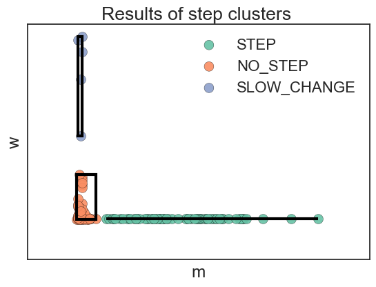
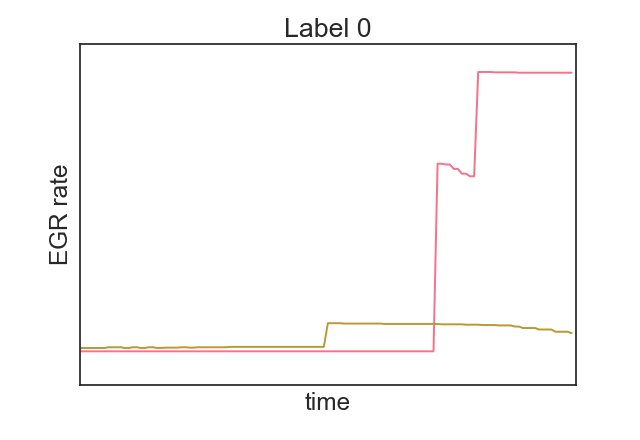
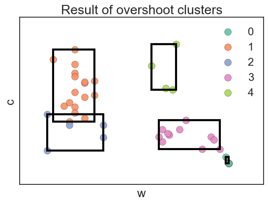
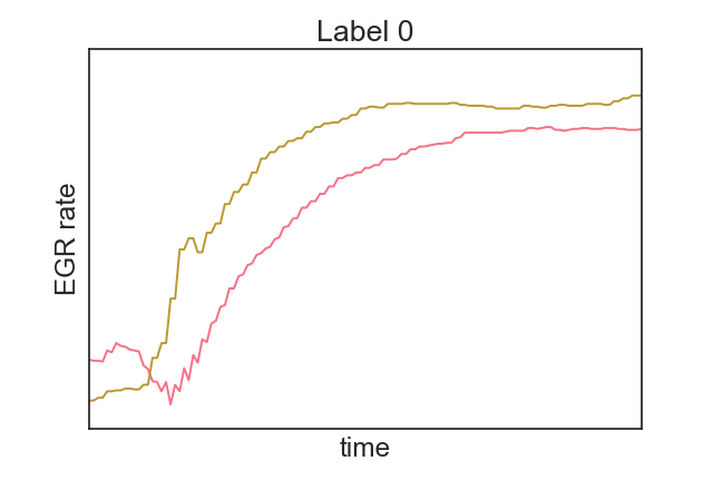
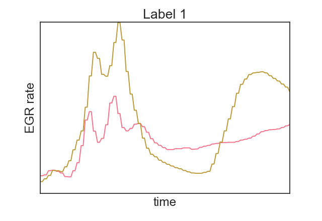
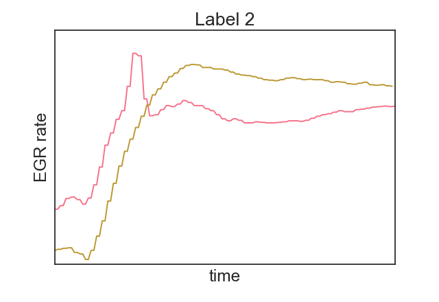
Results. The Step template revealed 3 clusters (Fig 5a), of which the cluster labeled Step (Fig 5b), was identified as an admissible “step” primitive. In picking the appropriate bounding box in we noted spikes have no inherit upper limit to their peaks. Thus, we derived the characterizing STL: , where are suppressed for proprietary reasons. The overshoot analysis revealed 5 clusters. We note that there are actually 2 distinct clusters which can reasonably be called overshoots, given by label 1 and 4 in Fig 5c. The interpretation, is that while the majority of the overshoots occur soon after the step, there is a cluster that occurred later, either due to slow rise time or non-linear effects causing the oscillation about the reference to increasing before dying away. In either case, as with spike, we declare that any overshoot is still an overshoot as the amplitude rises. Thus for cluster 1 we again chose to use a box from that does not bound . This lead to: again suppressing values.
Traffic Behavior on the US-101 highway. In order to model and predict driver behavior on highways, the Federal Highway Administration collected detailed traffic data on southbound US-101 freeway, in Los Angeles [8]. The pre-selected segment of the freeway is about 640 meters in length and consists of five main lanes and some auxiliary lanes. Traffic through the segment was monitored and recorded through eight synchronized cameras, mounted on top of the buildings next to the freeway. A total of minutes of traffic data was recorded including vehicle trajectory data providing lane positions of each vehicle within the study area.
heightadjust=object
| C | T | |C| | |||
|---|---|---|---|---|---|
| 0 | T1 | 626 | |||
| 1 | T2 | 115 | |||
| 2 | T2 | 44 | |||
| 3 | [.26, 30] | T3 | 52 | ||
| 4 | T2 | 32 | |||
| 5 | [.56, 54] | T3 | 14 | ||
| 6 | [.56, 32] | [1.8, 24] | T4 | 12 | |
| 7 | 76 | T1 | 1 |
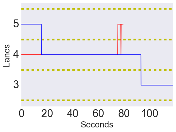
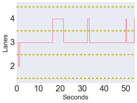
Here, we apply our method to analyze lane switching “aggressiveness” characterized by how often a driver switches lanes and the dwell time in each lane before switching. We focus on lanes 2, 3, and 4, ignoring the outer lanes lanes 1 and 5 since they are used entering and exiting the freeway, and thus have qualitatively different behavior. Each vehicle trajectory , stores the lane position for the vehicle, and we use the following STL formula to capture the dwell time in :
| (17) |
Results. For this experiment, from 4824 total vehicle trajectories, we discard trajectories with no lane switching behavior and group them with the conservative driving behaviors. We analyze the remaining 896 targeted trajectories that have at least one lane-switch behavior, and each trajectory is at most 100 seconds long. As all parameters are independent, lexicographic ordering has no impact on . After normalizing the parameters by centering and scaling, we apply GMMs to label and generate bounding hyperboxes/STL formulas.
The resulting clusters are shown in Table 6a. Upon examining the representatives,we classified the behaviors of each cluster into 4 groups:
-
•
T1: No Weaving: only switching to adjacent lanes and never changing back.
-
•
T2: Normal driving behavior, from switching to adjacent lanes and coming back to overtake a slow vehicle in front
-
•
T3: Slightly aggressive behavior, weaving between lanes.
-
•
T4: Aggressive behavior, weaving between all three lanes.
The largest cluster, 0, contains behaviors without any weaving behavior. Cluster 3 and 5 represent the weaving behavior involving 2 lanes. Cluster 6 represents aggressive behavior and one of the representative is shown in Fig. 6c. We consider Cluster 7 as an anomaly for Cluster 2 as it has only 1 trajectory.
For clusters 1, 2, and 4, we cannot distinguish if drivers were rapidly weaving or weaving within a short period of time, due to the scarcity of the data. As seen in Fig. 6b, the representatives for cluster , demonstrated two different behaviors; one involving rapid lane-switching (red trace), one where the driver switched lanes more slowly (blue trace). Applying an additional 1-class SVM to the points in cluster was used to distinguish these two cases.
CPS Grader. Massively Open Online Courses (MOOCs) present instructors the opportunity to learn from a large amount of collected data. For example, the data could be clustered to identify common correct solutions and mistakes. Juniwal et al. [16] demonstrated a semi-supervised procedure for a CPS MOOC; this involved first using DTW and K-Nearest Neighbors (KNN) to cluster traces of student solutions, and then picking representatives from clusters to ask the instructor to label. From the labeled data, they extract a characterizing STL formula given a PSTL template. The techniques demonstrated in this paper offer an alternative approach that can overcome some limitations of [16]. Firstly, as demonstrated in the opening example (see Fig. 1), DTW does not necessarily group traces in a way consistent with their logical classification. Second, the burden of labeling traces can still be quite large for instructors if the number of clusters is very large. Instead, unsupervised our approach offers a fully unsupervised approach (e.g., based on GMMs or K-Means) which still offers some degree of confidence that elements in the same cluster are similar w.r.t. a given PSTL template.
The tests in [16] involved the simulation of an IRobot Create and student generated controllers. The controller needed to navigate the robot up an incline and around static obstacles. To test this, the authors created a series of parameterized environments and a set of PSTL formula that characterized failure. In this work, we attempt to reproduce a somewhat arbitrary subset of the results shown in [16] that required no additional preprocessing on our part.
Obstacle Avoidance. We focus on 2 tests centered around obstacle avoidance. The authors used an environment where an obstacle is placed in front of a moving robot and the robot is expected to bypass the obstacle and reorient to it’s pre-collision orientation before continuing. The relevant PSTL formulas were “Failing simple obstacle avoidance” and “Failing re-orienting after obstacle avoidance” given below as and resp.:
| (18) | |||
| (19) |
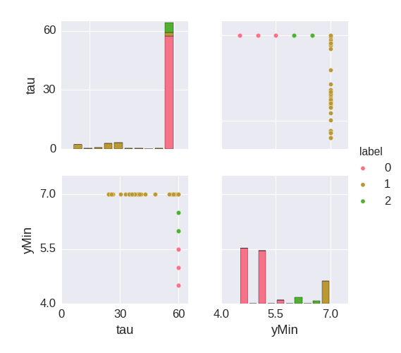
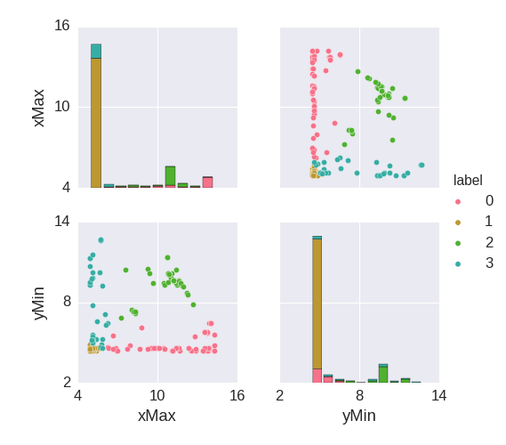
Results. A surprising observation for both templates is that
the vast majority of data is captured in a relatively small parameter
range. Upon investigation, it was revealed that the students were able
to submit multiple solutions for grading — each corresponding to a
trace. This biased the dataset towards incorrect solutions since one
expects the student to produce many incorrect solutions and then a few
final correct solutions. As seen in Fig. 7a, the
results imply that a classifier for label 0, which corresponded to the
robot not passing the obstacle, would have a low misclassification
rate when compared against the STL artifact from
[16]. Moreover, for obstacle avoidance, there
are two other families of correct solutions uncovered. One is the set
of traces that just barely pass the obstacle in time (label 2 in
Fig. 7a), and the other is the spectrum of
traces that pass the minimum threshold with a healthy margin (label 1
in Fig. 7a). For the reorient template, we
discovered 3 general types of behaviors (again with GMMs), see Fig. 7b. The first (label 1) is a failure to move past the
obstacle (echoing the large group under the obstacle avoidance
template). The other 3 groups seem to move passed the obstacle, but
two (labels 0 and 3) of them display failure to reorient to the
original orientation of . One could leverage this behavior
to craft diagnostic feedback for these common cases.
Conclusion. In this work we explored a technique
to leverage PSTL to extract features from a time series that can be
used to group together qualitatively similar traces under the lens of
a PSTL formula. Our approach produced a simple STL formula for each
cluster, which along with the extremal cases,
enable one to develop insights into a set of traces. We then
illustrated with a number of case studies how this technique could be
used and the kinds of insights it can develop. For future work, we
will study extensions of this approach to supervised, semi-supervised,
and active learning. A key missing component in this work is a
principled way to select a projection function (perhaps via learning
or posterior methods). Other possible extensions involve integration
with systematic PSTL enumeration, and learning non-monotonic PSTL
formulas.
References
- [1] Logical Clustering CAV2017 Artifact. https://archive.org/details/Logical_Clustering_CAV2017_Artifact, accessed: 2017-04-29
- [2] Ackerman, E.: Google’s Autonomous Cars Are Smarter Than Ever at 700,000 Miles. IEEE Spectrum (2014)
- [3] Akazaki, T., Hasuo, I.: Time robustness in MTL and expressivity in hybrid system falsification. In: International Conference on Computer Aided Verification. pp. 356–374. Springer (2015)
- [4] Alur, R., Henzinger, T.A.: A really temporal logic. JACM 41(1), 181–203 (1994)
- [5] Asarin, E., Donzé, A., Maler, O., Nickovic, D.: Parametric identification of temporal properties. In: Proc. of RV. pp. 147–160 (2011)
- [6] Bartocci, E., Bortolussi, L., Sanguinetti, G.: Learning temporal logical properties discriminating ECG models of cardiac arrhytmias. arXiv preprint arXiv:1312.7523 (2013)
- [7] Bombara, G., Vasile, C.I., Penedo, F., Yasuoka, H., Belta, C.: A Decision Tree Approach to Data Classification using Signal Temporal Logic. In: Proc. of HSCC. pp. 1–10 (2016)
- [8] Colyar, J., Halkias, J.: US highway 101 dataset. Federal Highway Administration (FHWA), Tech. Rep. FHWA-HRT-07-030 (2007)
- [9] Donzé, A.: Breach, a toolbox for verification and parameter synthesis of hybrid systems. In: Proc. of CAV. pp. 167–170 (2010)
- [10] Donzé, A., Maler, O., Bartocci, E., Nickovic, D., Grosu, R., Smolka, S.: On temporal logic and signal processing. In: Proc. of ATVA. pp. 92–106. Springer (2012)
- [11] F. Pedregosa, et al.: Scikit-learn: Machine Learning in Python. Journal of Machine Learning Research 12, 2825–2830 (2011)
- [12] Hoxha, B., Dokhanchi, A., Fainekos, G.: Mining parametric temporal logic properties in model-based design for cyber-physical systems. International Journal on Software Tools for Technology Transfer pp. 1–15 (2017)
- [13] J. Kapinski et al.: ST-Lib: A Library for Specifying and Classifying Model Behaviors. In: SAE Technical Paper. SAE (2016)
- [14] Jin, X., Donzé, A., Deshmukh, J.V., Seshia, S.A.: Mining requirements from closed-loop control models. IEEE TCAD of ICS 34(11), 1704–1717 (2015)
- [15] Jones, A., Kong, Z., Belta, C.: Anomaly detection in cyber-physical systems: A formal methods approach. In: Proc. of CDC. pp. 848–853 (2014)
- [16] Juniwal, G., Donzé, A., Jensen, J.C., Seshia, S.A.: CPSGrader: Synthesizing temporal logic testers for auto-grading an embedded systems laboratory. In: Proc. of EMSOFT. p. 24 (2014)
- [17] Keogh, E.J., Pazzani, M.J.: Scaling up dynamic time warping for data mining applications. In: Proc. of KDD. pp. 285–289 (2000)
- [18] Kong, Z., Jones, A., Medina Ayala, A., Aydin Gol, E., Belta, C.: Temporal logic inference for classification and prediction from data. In: Proc. of HSCC. pp. 273–282 (2014)
- [19] Koymans, R.: Specifying real-time properties with metric temporal logic. Real-time systems 2(4), 255–299 (1990)
- [20] Legriel, J., Le Guernic, C., Cotton, S., Maler, O.: Approximating the pareto front of multi-criteria optimization problems. In: Proc. of TACAS. pp. 69–83 (2010)
- [21] Li, W., Forin, A., Seshia, S.A.: Scalable specification mining for verification and diagnosis. In: Proceedings of the Design Automation Conference (DAC). pp. 755–760 (June 2010)
- [22] Lin, J., Keogh, E., Truppel, W.: Clustering of streaming time series is meaningless. In: Proceedings of the 8th ACM SIGMOD workshop on Research issues in data mining and knowledge discovery. pp. 56–65. ACM (2003)
- [23] Maler, O., Nickovic, D.: Monitoring temporal properties of continuous signals. In: Proc. of FORMATS/FTRTFT. pp. 152–166 (2004)
- [24] Von Luxburg, U.: A tutorial on spectral clustering. Statistics and computing 17(4), 395–416 (2007)
6 Appendix
Related monotonic formula for a non-monotonic PSTL formula.
Example 9
Consider the PSTL template: . We first show that the given formula is not monotonic.
Proof
Consider the trace . Keep fixed . Observe that , satisfies the formula. If , then , since is not eventually satisifed. If , then implying that for satisfaction, within the next 1 time units, the signal must becomes greater than 1. The signal is always 0, so at , the formula is unsatisfied. Thus, while increasing from to to , the satifaction has changed signs twice. Thus, is not monotonic.
Now consider the following related PSTL formula in which repeated instances of the parameter are replaced by distinct parameters and . We observe that this formula is trivially monotonic:
Linearization based on scalarization.
Borrowing a common trick from multi-objective optimization, we define a cost function on the space of valuations as follows: . Here, , are weights on each parameter. The above cost function implicitly defines an order , where, iff . Then, the projection operation is defined as: . We postpone any discussion of how to choose such a scalarization to future work.