RRT⁺: Fast Planning for High-Dimensional Configuration Spaces

Abstract

In this paper we propose a new family of RRT based algorithms, named RRT⁺, that are able to find faster solutions in high-dimensional configuration spaces compared to other existing RRT variants by finding paths in lower dimensional subspaces of the configuration space. The method can be easily applied to complex hyper-redundant systems and can be adapted by other RRT based planners. We introduce RRT⁺ and develop some variants, called PrioritizedRRT⁺, PrioritizedRRT⁺-Connect, and PrioritizedBidirectionalT-RRT⁺, that use the new sampling technique and we show that our method provides faster results than the corresponding original algorithms. Experiments using the state-of-the-art planners available in OMPL show superior performance of RRT⁺ for high-dimensional motion planning problems.

I Introduction

Despite the dramatic development of robotics in recent decades, robots are still far from outperforming humans in operations for which they are not specialized, however few types of robots are capable of completing generic tasks. Complex robots such as mobile manipulators, snake robots, or humanoids have been presented mostly in experimental contexts. While the fact that a human adult has 244 degrees of freedom [1], emphasizes the need for such complicated systems, which would compare favorably with human performance in many domains.

This study focus on the path planning problem in high-dimensional configuration spaces and aims to provide a new family of motion planners that generate faster solutions than other RRT-based motion planners. The approach is based on the observation that for many hyper-redundant systems, it is rare for all the kinematic abilities of the system to be needed for a certain task [2].

Figure 1: Solution for a 30-DOF kinematic chain in a highly constrained horn environment using the proposed algorithm.

In this paper, a novel RRT-based family of algorithms, termed RRT⁺, is presented. These algorithms incrementally search in subspaces of the configuration space $\mathcal{C}$. The modifications are not only related to the sampler but also to the way the RRT is expanded since the entire search is separated into a series of subsearches, confined to subspaces of increasing dimensionality.

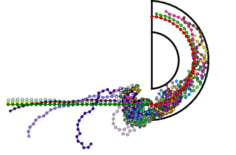
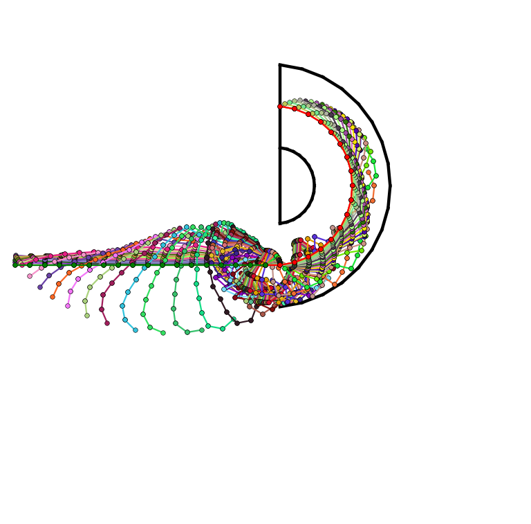
We show that these algorithms keep all the theoretical guarantees of the original RRT algorithms, while at the same time can provide much faster solutions in many cases. Moreover, the idea can easily be grafted to other motion planners — in the authors’ experience, sometimes in just a few minutes of programming — resulting in significant increases in performance. Furthermore, the efficiency can be significantly increased by having prior information about the system. Figure 1 presents an example plan for a 30 DoF manipulator in a tight environment computed by one of the proposed algorithms, namely PrioritizedRRT⁺-Connect.

The remainder of this paper is structured as follows, related work and other approaches to these problems is discussed in Section II. The problem statement is in Section III and the proposed algorithm is presented in Section IV. Section V presents experiments comparing RRT⁺ to five other state-of-the-art planners from OMPL. Finally, the paper concludes with a discussion of future work in Section VI.

II Related work

The problem of the motion planning has been proven to be PSPACE-hard [3]. Building robotic systems with high-dimensional configuration spaces is a field that many studies have been done for different type of systems. Generally there are four big categories: hyper-redundant manipulators, mobile manipulators, cooperative robotic systems and humanoids. We are going to present some of the important studies on those systems.

There are some works that show applications of hyper-redundant systems as demonstrated by Ma et al. [4] who developed a hyper-redundant arm in order to make real time and precise operations inside nuclear reactors. Liljeback et al. [5] created a snake fire-fighting hyper-redundant robot, and Ikuta et al. [6] used a 9-DoF arm to operate during surgeries in deep areas.

There are also few works for mobile manipulators and multi-robot systems from the early 90’s. The inverse kinematics for mobile manipulators where solved and optimal solutions were obtained with guarantees of safe performance in the study of Dubowsky and Vance [7]. Later studies were presented, such as the one of Yamamoto and Yun [8] where an algorithm for maximizing the manipulability was presented, and the work of Khabit et al. [9] introduced an algorithm for cooperative systems of mobile manipulators. As for the cooperative systems, some early efforts include the works of Buckley [10] and Cao et al. [11].

From late 90’s, sampling-based methods were introduced and shown to be capable of solving challenging motion planning problems, but without guaranties for finding the solution in finite time [12]. The two most famous representatives of those algorithms are probabilistic roadmaps (PRMs) by Kavraki et al. that require preprocessing and a known, generally stable, environment [13] and RRTs by LaValle [14], that are more suitable for single query applications. Although the performance of both these techniques can be affected substantially by the number of the degrees of freedom, some studies have use them successfully for high-dimensional configuration spaces.

A method that uses PRM was presented by Park et al. [15] that finds collision-free paths for hyper-redundant arms. Other studies use RRTs for motion planning of redundant manipulators, such as the work of Bertram et al. [16], which solves the inverse kinematics in a novel way. Weghe et al. [17] apply RRT to redundant manipulators without the need to solve the inverse kinematics of the system. A study by Qian and Rahmani [18] combines the RRT and the inverse kinematics in a hybrid algorithm in a way that drives the expansion of the RRT by the Jacobian pseudo-inverse.

Additionally, some works use RRTs for mobile manipulators. Vannoy et al. [19] proposes an efficient and flexible algorithm for operating in dynamic environments. The work of Berenson et al. [20] provides an application of their technique to a 10-DoF mobile manipulator.

For multi-robot systems, many sampling-based algorithms have been proposed. The study of van den Berg and Overmars [21] uses a PRM and presents a prioritized technique for motion planning of multiple robots. Other studies use RRT-based algorithms such as the study by Carpin and Pagello [22] which introduced the idea of having multiple parallel RRTs for multi-robot systems, or the work of Wagner [23] that plans for every robot individually and the it tries to coorbinate the motion if needed in higher dimensional spaces. Other studies propose efficient solutions by using a single RRT [24, 25]. There is also some work on humanoid robots with sampling-based algorithms; Kuffner et al. presented algorithms for motion planning on humanoid robots with both the use of PRMs [26] and RRTs [27]. Other studies, such as the work of Liu et al. [28], which used RTTs for solving the stepping problem for humanoid robots.

The work of Vernaza and Lee tried to extract structural symmetries in order to reduce the dimensionality of the problem [29] by also providing near-optimal solutions. This technique is more time efficient than the traditional RRT only for very high-dimensional configuration spaces. Yershova et al. [30] proposed an approach to focus the sampling in the most relevant regions.

Finally, some other approaches attempt to deal with the curse of dimensionality in different ways. Gipson et al. developed STRIDE[31] which samples non-uniformly with a bias to unexplored areas of $\mathcal{C}$. Additionally, Gochev et al. [32] proposed a motion planner that decreases the dimensionality by recreating a configuration space with locally adaptive dimensionality. Yoshida’s work [33] tries to sample in ways that exploit the redundancy of a humanoid system. Kim et al. [34] present an RRT-based algorithm for articulated robots that reduces the dimensionality of the problem by projecting each sample into subspaces that are defined by a metric. Shkolnik and Tedrake  [35] plan for high redundant manipulators in the a dimensional task space with the use of Jacobian transpose and Vornoi bias. Last it is worth to mention the work of Bayazitet al. [36] where a PRM was used to plan in subspaces of $\mathcal{C}$, creating paths that solve an easier problem than the original and then iteratively optimize the solution by extending the subspace till it finds a valid solution.

This paper provides a general and simple to implement RRT-based family of algorithms for efficient motion planning for arbitrary hyper-redundant systems, regardless if there is an articulated robot, or a humanoid, or an heterogeneous multi-robot system. unlike the previous works, the algorithm tries to find paths that are not only confined entirely in a global subspace but also in a subspace in which a solution can exist, since the initial and goal configurations are part of the same subspace. The algorithm not only exploits redundancy but also can provide fast solutions that satisfy some constraints by simply searching in subspaces where those constraints are satisfied. Contrary to  [36] the algorithm searches in subspaces that are strictly lower-dimensional and instead of solving an easier problem than the original, since refining the tree will be costly for an RRT, it tries to solve a much more difficult problem by applying virtual constraints, and iteratively relaxes those virtual constraints. The algorithm is easily applicable to a variety RRT-based motion planners; we demonstrate this property by applying one variant of our method to RRT [14], RRTConnect [37] and Bidirectional T-RRT [38].

III Problem Statement

Let $\mathcal{C}$ denote a configuration space with $n$ degrees of freedom, partitioned into free space $\mathcal{C}_{\textrm{free}}$ and obstacle space $\mathcal{C}_{\textrm{obs}}$ with $\mathcal{C}=\mathcal{C}_{\textrm{free}}\cup\mathcal{C}_{\textrm{obs}}$. The obstacle space $\mathcal{C}_{\textrm{obs}}$ is not explicitly represented, but instead can be queried using collision checks on single configurations or short path segments. Given initial and goal configurations $q_{\rm init},q_{\rm goal}\in\mathcal{C}_{\textrm{free}}$, we would like to find a continuous path in within $\mathcal{C}_{\rm free}$ from $q_{\rm init}$ to $q_{\rm goal}$.

For purposes of sampling, we assume that each degree of freedom in $\mathcal{C}$ is parameterized as an interval subset of $\mathbb{R}$, so that

$$\mathcal{C}=\left[c_{1}^{\rm(min)},c_{1}^{\rm(max)}\right]\times\dots\times\left[c_{n}^{\rm(min)},c_{n}^{\rm(max)}\right]\subseteq\mathbb{R}^{n}.$$ (1)

Note that we treat $\mathcal{C}$ as Euclidean only in the context of sampling; other operations such as distance calculations and generation of local path segments utilize identifications on the boundary of $\mathcal{C}$ as appropriate for the topology.

IV Algorithm description

IV-A The RRT⁺ Algorithm

The proposed family of algorithms is based on attempting to find a solution in lower dimensional subspace of $\mathcal{C}$, in hopes that such a path might be found faster than expanding the tree in all dimensions. The underlying idea is to exploit the redundancy of each system for each problem. To achieve this, the algorithm starts searching in a 1-dimensional subspace of $\mathcal{C}$ that contains $q_{\rm init}$ and $q_{\rm goal}$. If this search fails, the algorithm expands its search subspace by one dimension. This process continues iteratively until the algorithm finds a path, or until it searches in all of $\mathcal{C}$. During all the different searches, also called sub-searches, the tree structure is kept and expanded in subsequent stages.

Input : A configuration space $\mathcal{C}$, an initial configuration $q_{\rm init}$, and a goal configuration $q_{\rm goal}$.

Output : RRT graph $G$

1

2$G$.init($q_{init}$)

3 $\mathcal{C}_{\textrm{sub}}\leftarrow$ 1-d subspace of $\mathcal{C}$, through $q_{init}$ and $q_{goal}$

4

5while True do

6       $q_{\rm rand}\leftarrow$ sample drawn from $\mathcal{C}_{\textrm{sub}}$

7       $q_{\rm near}\leftarrow$NearestVertex$(q_{\rm rand},G)$

8       $q_{\rm new}\leftarrow$NewConf$(q_{\rm near},q_{\rm rand})$

9       $G$.AddVertex($q_{\rm new}$)

10       $G$.AddEdge($q_{\rm near}$, $q_{\rm new}$)

11       if done searching $\mathcal{C}_{\textrm{sub}}$ then

12             if $\dim(\mathcal{C}_{\textrm{sub}})<\dim(\mathcal{C})$ then

13                   Expand $\mathcal{C}_{\textrm{sub}}$ by one dimension.

14             else

15                   return $G$

16             end if

17            

18       end if

19      

20 end while

Algorithm 1 RRT⁺

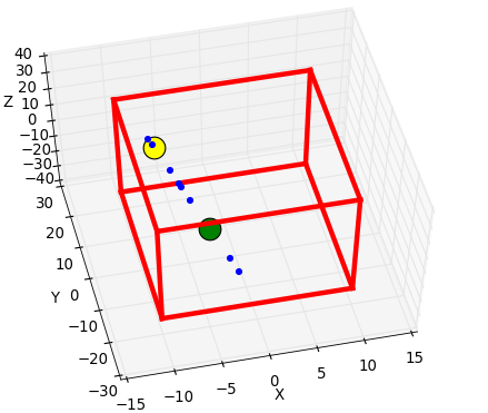
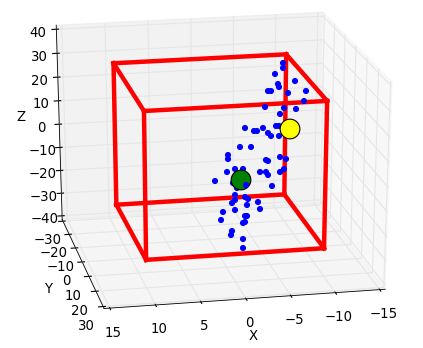
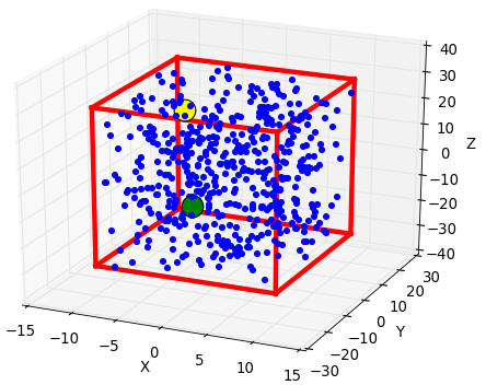
Algorithm 1 summarizes the approach. The planner starts optimistically by searching in one dimension, along the line passing through $q_{\rm init}$ and $q_{\rm goal}$. If this search fails to find a path—a certainty, unless there are no obstacles between $q_{\rm init}$ and $q_{\rm goal}$—the search expands to a planar subspace that includes $q_{\rm init}$ and $q_{\rm goal}$, then to a 3D hyperplane, and so on until, in the worst case, the algorithm eventually searches all of $\mathcal{C}$; see Fig. 2.

For simplicity, the pseudocode in Algorithm 1 shows a straightforward, single-directional RRT⁺, analogous to the standard vanilla RRT. Note, however, the idea readily applies to most tree-based motion planners, since primary difference is in how the samples are generated. The experiments in Section V, for example, describe RRT⁺ planners based on the well-known goal biased and bidirectional RRT algorithms.

Figure 2: Sampling in one, two and three dimensions in $\mathcal{C}$.

The description in Algorithm 1 leaves three important elements unspecified. First, the algorithm needs a method for selecting and representing the subspace $\mathcal{C}_{\textrm{sub}}$ (Lines 1 and 1). Next, we must provide a method for sampling from this subspace (Line 1). Finally, we must decide upon the conditions that must be met before moving to the next subsearch (Line 1). Particular choices for each of these elements can be based on knowledge about the specific types of problems being solved; this freedom is why we refer to RRT⁺ as a family of algorithms. Sections IV-B, IV-C, and IV-D describe some possibilities for instantiating the basic framework. Section IV-E establishes conditions under which the resulting planner is probabilistically complete.

IV-B Choosing and representing subspaces

The central idea is to search for solutions in subspaces of progressively higher dimensions. The primary constraint on these subspaces is that they must contain both $q_{\rm init}$ and $q_{\rm goal}$; subspaces that violate this constraint cannot, of course, contain a path connecting $q_{\rm init}$ to $q_{\rm goal}$.

In general, the algorithm’s selections for $\mathcal{C}_{\textrm{sub}}$ should ideally be directed by the likelihood that a solution will exist fully within $\mathcal{C}_{\textrm{sub}}$, but in the absence of useful heuristics for predicting this success, simple randomness may be quite effective, especially for highly-redundant systems. The next examples illustrate some options.

Example 1

A natural choice is to let $\mathcal{C}_{\textrm{sub}}$ be an affine subspace of $\mathcal{C}$. That is, we select at random a flat in $\mathcal{C}$ passing through $q_{\rm init}$ and $q_{\rm goal}$.

Example 2

Another possibility is to use for $\mathcal{C}_{\textrm{sub}}$ a convex polytope. That is, we select a collection of points $q_{1},\ldots,q_{m}\in\mathbb{R}^{n}$ whose convex hull contains both $q_{\rm init}$ and $q_{\rm goal}$, and define $\mathcal{C}_{\textrm{sub}}$ as a the set of all convex combinations of those points.

Example 3

A final possibility —one that trades some generality for simplicity— is a prioritized release of the degrees of freedom. Given a set $P_{\rm con}\subseteq\{1,\ldots,n\}$ of degrees of freedom to be constrained, we can form $\mathcal{C}_{\textrm{sub}}$ by constaining the degrees of freedom in $P_{\rm con}$ to form a line passing from $q_{\rm init}$ and $q_{\rm goal}$ and allowing the remaining DoFs to vary freely.

IV-C Sampling from the subspaces

Next, the algorithm requires a technique for drawing samples from $\mathcal{C}_{\textrm{sub}}$.

Example 4

For affine subspaces represented as in Example 1, samples in $\mathcal{C}_{\textrm{sub}}$ can be generated by selecting a random vector $r\in\mathbb{R}^{s}$, and applying an affine transformation:

$$q_{\rm rand}=Ar+q_{\rm init}.$$ (2)

The main difficulty is to ensure that the resulting $q$ lies inside the C-space as defined in Equation 1. Possibilities for handling this difficult include rejection sampling, computing the portion of $\mathbb{R}^{s}$ that maps into $\mathcal{C}$ and generating $r$ from that region, or simply allowing samples to fall outside of $\mathcal{C}_{\textrm{sub}}$, and tolerating the potential distortion this would induce to the growth of the tree.

Example 5

With the formulation described in Example 2, uniform samples from the convex hull of $q_{1},\ldots,q_{m}$ can be generated using the algorithms of Linial [39] or Trikalinos and Valkenhoef [40].

Example 6

Prioritized sampling as described in Example 3, a very efficient linear time method to produce samples is by initially generating a sample within $\mathcal{C}$ along the line between $q_{\rm init}$ and $q_{\rm goal}$ by selecting a random scalar $r$ and applying:

$$q_{\rm rand}^{(i)}=(q_{\rm goal}^{(i)}-q_{\rm init}^{(i)})r+q_{\rm init}^{(i)}$$ (3)

The algorithm then modifies $q_{\rm rand}$ by inserting, for each DoF not in $P_{\rm con}$, a different random value within the range for that dimension; see Algorithm 2.

Input : Initial configuration $q_{\rm init}$, goal configuration $q_{\rm goal}$, set of constrained DoF $P_{\rm con}$

Output : Sample configuration $q$

1

2$q\leftarrow$ random point in $\mathcal{C}$ along line from $q_{\rm init}$ to $q_{\rm goal}$

3 for $s\in 1,\ldots,n$ do

4       if $s\notin P_{\rm con}$ then

5             $q[s]\leftarrow$ Random($0$, $1$)$*(c^{(max)}_{s}-c^{(min)}_{s})+c^{(min)}_{s}$

6            

7       end if

8      

9 end for

10

11return $q$

Algorithm 2 Prioritized Sampler

While this approach is simple, it loses some generality since only a finite number of flats can be explored; given specific $q_{\rm init}$, $q_{\rm goal}$, and $P_{\rm con}$ the subspaces are fully determined.

IV-D Terminating the subsearches

The only remaining detail to be discussed is for how long the search in the each subspace should continue. There are multiple ways to deal with this problem and good online heuristics can be found, but for simplicity in this paper we assume that there is a fixed number of samples $k_{i}$ for iteration $i$. Algorithm 3 presents a technique for selecting the $k_{i}$ values, based on a maximum number of total samples $Q_{\rm total}$. The idea is to exponentially increase the number of samples in each successive subsearch, acknowledging the need for more samples in higher dimensions.

Input : The total number of samples $Q_{\rm total}$, dimension of configuration space $n$.

Output : $k_{1},\ldots,k_{n}$

1

2$v\leftarrow\exp{\frac{\ln{Q_{\rm total}}}{n}}$

3 for $s\leftarrow 1,\ldots,n$ do

4       $k_{s}\leftarrow v^{s}$

5      

6 end for

7return $k_{1},\ldots,k_{n}$

Algorithm 3 FindSampleSize

For the sake of simplicity if we assume that $v_{i}=v$, for some constant $v$, then the number of samples for each $j$ step will be:

$$k_{j}=v^{j}$$ (4)

The total number of samples $Q_{\rm total}$ for all the steps will be the sum of the above geometric sequence:

$$Q_{\rm total}=\sum_{j=1}^{n}{v^{j}}=\frac{v(v^{n}-1)}{v-1}$$ (5)

It can be shown that in the unlikely worst case the RRT⁺ algorithm would be slightly slower than the regular RRT since:

$$Q_{max}\leq\frac{v(Q_{max}-1)}{v-1}\approx\frac{v}{v-1}Q_{max}$$ (6)

Also it is important that the efficiency of the algorithm in the worst case, is strongly related to the value of $v$. For bigger values of $v$, so bigger values of $Q_{\rm total}$, the difference in the efficiency in the worst case is reduced. So by setting as $Q_{max}$ the average number of samples that the algorithm before the application of the method the new algorithm succeeds on even in the worst uncommon case for a hyper-redundant system, having similar performance.

Last, putting everything together, the PrioritizedRRT⁺, based on Examples 3 and 6, is presented in Algorithm 4.

Input : Initial configuration $q_{\rm init}$, goal configuration $q_{\rm goal}$, number of samples $Q_{\rm total}$.

Output : RRT graph $G$

1

2$P_{con}\leftarrow$ $\{1,2,\dots,n\}$

3 $G$.init($q_{init}$)

4 $K\leftarrow$ FindSampleSize($N$, $S$)

5 for $s\leftarrow 1,\ldots,n$ do

6       for $i\leftarrow 1,k_{s}$ do

7             $q_{\rm rand}\leftarrow$PrioritizedSampler($S$, $q_{\rm init}$, $q_{\rm goal}$, $P_{\rm con}$)

8             $q_{\rm near}\leftarrow$NearestVertex$(q_{\rm rand},G)$

9             $q_{\rm new}\leftarrow$NewConf$(q_{\rm near},q_{\rm rand})$

10             $G$.AddVertex($q_{\rm new}$)

11             $G$.AddEdge($q_{\rm near}$, $q_{\rm new}$)

12            

13       end for

14      Extract($P_{\rm con}$)

15      

16 end for

return $G$ 

Algorithm 4 Prioritized RRT⁺

In Fig. 2, the visual result of the sampler for a 3-dimensional configuration space and the three different states, with $Q_{max}=512$. The initial state is shown as a yellow ball; the goal state is shown as a green ball, and the red lines indicate the boundary of $\mathcal{C}$.

IV-E Probabilistic Completeness

Theorem 1

The RRT⁺ is probabilistically complete if the following conditions hold.

• $\mathcal{C}_{\textrm{sub}}$ in the last stage is the entire $\mathcal{C}$.

• The sampler can generate any point in $\mathcal{C}_{\textrm{sub}}$.

• In each stage before the final stage, only a finite number of samples is generated.

Proof:

Under these conditions, RRT⁺ is guaranteed to reach its last iteration in finite time. In this final iteration, the algorithm behaves in the exact same way as the RRT, so RRT⁺ inherits the probabilistic completeness of RRT. ∎

V Experiments

For the experiments three new planners in the RRT⁺ family were developed in within OMPL [41]. These planners work by applying the prioritized technique to three RRT variants: (1) RRT with goal bias of $0.5$. (2) RRT-Connect and (3) the bidirectional T-RRT [38]. The T-RRT variant is intended to demonstrate the applicability of the idea to a powerful costmap planner.

In order to show the ability of the new planners to adapt in different problems, the prioritization was chosen randomly for each run, although an optimization might be expected to give faster results. For implementation reasons, the parameter $Q_{max}$ was specified not by indicating the number of the samples, but the total desired time the subsearch should be done to a machine with 6th Generation Intel Core i7-6500U Processor (4MB Cache, up to 3.10 GHz) and 16GB of DDR3L (1600MHz) RAM. As expected the performance proved to be sensitive to this parameter.

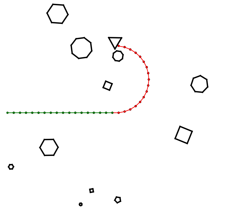
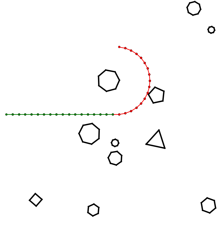
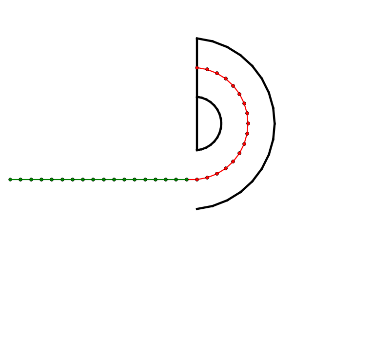
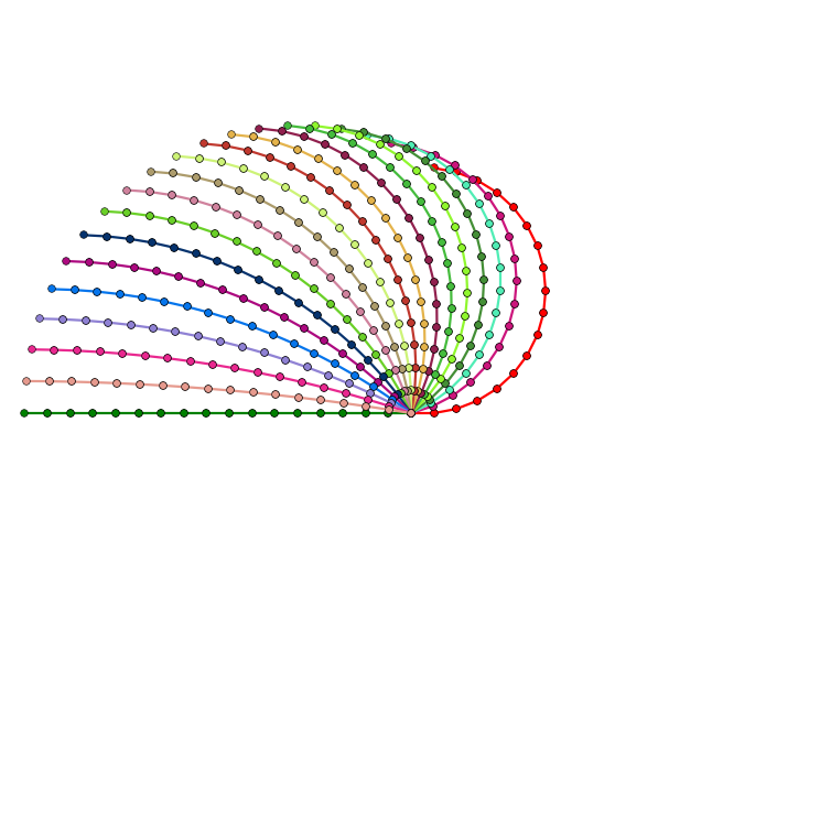
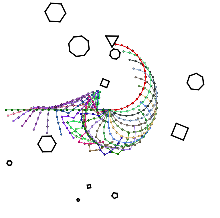
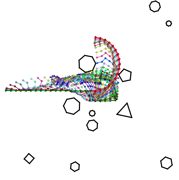
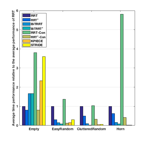
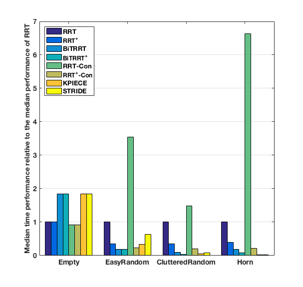
Four different environments were tested 100 times each for a 17-DoF kinematic chain, with decreasing redundancy: The Empty environment, a Random Easy environment, a more Cluttered Random environment, and the Horn environment; see Fig. 3. In all the cases, the RRT⁺ versions of each planner were faster and in most cases significantly faster. Details appear in Fig. 4 and Table I.

As can be observed, the PrioritizedRRT⁺-Connect not only outperformed the RRT-Connect by a wide margin, but also all the other planners using uniform sampling. Additionally, it outperformed robust planners with biased sampling in environments with more redundancy, but KPIECE [42] and STRIDE [31] are the clear winners in less redundant problems.

Interestingly, for each problem, the single fastest solution across all trials was generated by PrioritizedRRT⁺-Connect. This suggests a good choice of prioritization may give faster results in a consistent way.

Figure 3: The four different environments the Empty, the Easy Random, the Cluttered Random and the Horn (a-d) with red indicating the $q_{\rm init}$ and green the $q_{\rm goal}$, and four different solutions for those environments (e-h) with PrioritizedRRT⁺-Connect respectively.

Figure 4: The mean 4 and the median 4 for the four environments and the eight planners scaled by the execution time of the RRT. Please refer to Fig. 3 for the four test-environments and to Table I for the numerical values of the mean and standard deviation performance of the eight planners. Note that ⁺ indicate the proposed algorithms.

TABLE I: Averages with standard deviation in the 4 environments and for 100 runs for every planner in seconds.

	Empty	Easy Random	Cluttered Random	Horn
RRT	0.0015$\pm$ 0.0004	0.2134$\pm$ 0.3551	14.1118$\pm$ 16.8046	11.4807$\pm$ 12.2223
RRT+	0.0012$\pm$ 0.0002	0.0658$\pm$ 0.1268	7.0245$\pm$ 11.3234	7.2384$\pm$ 10.8390
BiTRRT	0.0025$\pm$ 0.0036	0.0306$\pm$ 0.0721	1.4039$\pm$ 1.7033	1.7877$\pm$ 2.2717
BiTRRT+	0.0025$\pm$ 0.0009	0.0179$\pm$ 0.02	0.3434$\pm$ 0.4004	0.9814$\pm$ 1.5429
RRT-Con	0.0057$\pm$ 0.0173	0.2924$\pm$ 0.7734	14.5406$\pm$ 11.1380	66.7144$\pm$ 76.6271
RRT+-Con	0.0012$\pm$ 0.0001	0.0267$\pm$ 0.0282	4.6150$\pm$ 12.4115	4.7672$\pm$ 8.9909
KPIECE	0.0035$\pm$ 0.0026	0.0315$\pm$ 0.0223	0.5744$\pm$ 0.51	0.1537$\pm$ 0.1153
STRIDE	0.0054$\pm$ 0.0044	0.0656$\pm$ 0.0529	0.8630$\pm$ 0.75	0.1800$\pm$ 0.4681

VI Conclusion

We presented a general novel family of algorithms for fast motion planning in high dimensional configuration spaces. The algorithm should provide in the common case faster solutions than the regular RRT based methods, though in the uncommon worst case the solutions are somewhat slower.

The algorithm is general enough to be applied to a broad variety of motion planning problems. For example, our experiments show potential for planning with costmaps via adaptation of the bidirectional TRRT. The planner also can be adjusted to each problem and provide faster results than the regular versions of the planners.

A number of important question remain unanswered. For example, it would be very interesting to find an efficient way to pick, while searching, subspaces that are more likely to contain solutions. Also, it is important to provide a general way to identify when a new iteration should begin, using a metric of the expansion of the tree, and eliminate the sensitivity to the $Q_{\rm max}$ parameter. Moreover, by using the previous metric it is possible to identify when the tree overcame a difficult area and then reduce the dimensionality of the search, in order to accelerate the results further.

Currently, there are two planners in OMPL that outperform the PrioritizedRRT⁺: KPIECE and STRIDE, which sample non-uniformly with a bias to narrow spaces. The integration of the ideas underlying RRT⁺ into those planners to accelerate the results is left for a future work.

Lastly, we plan to explore in the future the ability of the planner to efficiently produce paths that satisfy some natural constraints of each system.

References

- [1] A. D. Kuo, “A mechanical analysis of force distribution between redundant, multiple degree-of-freedom actuators in the human: Implications for the central nervous system,” Human movement science, vol. 13, no. 5, pp. 635–663, 1994.
- [2] M. Xanthidis, K. J. Kyriakopoulos, and I. Rekleitis, “Dynamically efficient kinematics for hyper-redundant manipulators,” in The 24th Mediterranean Conf. on Control and Automation, Athens, Greece, Jun. 2016, pp. 207–213.
- [3] J. Reif and M. Sharir, “Motion planning in the presence of moving obstacles,” Journal of the ACM, vol. 41, no. 4, pp. 764–790, 1994.
- [4] S. Ma, S. Hirose, and H. Yoshinada, “Development of a hyper-redundant multijoint manipulator for maintenance of nuclear reactors,” Advanced robotics, vol. 9, no. 3, pp. 281–300, 1994.
- [5] P. Liljeback, O. Stavdahl, and A. Beitnes, “Snakefighter-development of a water hydraulic fire fighting snake robot,” in 9th Int. Conf. on Control, Automation, Robotics and Vision, (ICARCV), 2006, pp. 1–6.
- [6] K. Ikuta, T. Hasegawa, and S. Daifu, “Hyper redundant miniature manipulator” hyper finger” for remote minimally invasive surgery in deep area,” in IEEE Int. Conf. on Robotics and Automation, vol. 1, 2003, pp. 1098–1102.
- [7] S. Dubowsky and E. Vance, “Planning mobile manipulator motions considering vehicle dynamic stability constraints,” in IEEE Int. Conf. on Robotics and Automation, 1989, pp. 1271–1276.
- [8] Y. Yamamoto and X. Yun, “Coordinating locomotion and manipulation of a mobile manipulator,” in Proc. of the 31st IEEE Conf. on Decision and Control, 1992, pp. 2643–2648.
- [9] O. Khatib, K. Yokoi, K. Chang, D. Ruspini, R. Holmberg, and A. Casal, “Vehicle/arm coordination and multiple mobile manipulator decentralized cooperation,” in Proc. of the IEEE/RSJ Int. Conf. on Intelligent Robots and Systems, vol. 2, 1996, pp. 546–553.
- [10] S. J. Buckley, “Fast motion planning for multiple moving robots,” in IEEE Int. Conf. on Robotics and Automation, 1989, pp. 322–326.
- [11] Y. U. Cao, A. S. Fukunaga, and A. Kahng, “Cooperative mobile robotics: Antecedents and directions,” Autonomous robots, vol. 4, no. 1, pp. 7–27, 1997.
- [12] S. M. LaValle, Planning Algorithms. Cambridge Univ. press, 2006.
- [13] L. E. Kavraki, P. Švestka, J.-C. Latombe, and M. H. Overmars, “Probabilistic roadmaps for path planning in high-dimensional configuration spaces,” IEEE Trans. on Robotics and Automation, vol. 12, no. 4, pp. 566–580, 1996.
- [14] S. M. LaValle, “Rapidly-exploring random trees: A new tool for path planning,” Computer Science Dept., Iowa State University, Tech. Rep. TR 98-11, Oct. 1998.
- [15] J. J. Park, H. S. Kim, and J.-B. Song, “Collision-free path planning for a redundant manipulator based on prm and potential field methods,” Journal of Institute of Control, Robotics and Systems, vol. 17, no. 4, pp. 362–367, 2011.
- [16] D. Bertram, J. Kuffner, R. Dillmann, and T. Asfour, “An integrated approach to inverse kinematics and path planning for redundant manipulators,” in Proc. IEEE Int. Conf. on Robotics and Automation, 2006, pp. 1874–1879.
- [17] M. V. Weghe, D. Ferguson, and S. S. Srinivasa, “Randomized path planning for redundant manipulators without inverse kinematics,” in 7th IEEE-RAS Int. Conf. on Humanoid Robots, 2007, pp. 477–482.
- [18] Y. Qian and A. Rahmani, “Path planning approach for redundant manipulator based on jacobian pseudoinverse-rrt algorithm,” in 6th Int. Conf. on Intelligent Robotics and Applications, Busan, South Korea, Sep. 2013, pp. 706–717.
- [19] J. Vannoy and J. Xiao, “Real-time adaptive motion planning (ramp) of mobile manipulators in dynamic environments with unforeseen changes,” IEEE Trans. on Robotics, vol. 24, no. 5, pp. 1199–1212, 2008.
- [20] D. Berenson, J. Kuffner, and H. Choset, “An optimization approach to planning for mobile manipulation,” in IEEE Int. Conf. on Robotics and Automation, 2008, pp. 1187–1192.
- [21] J. P. Van Den Berg and M. H. Overmars, “Prioritized motion planning for multiple robots,” in IEEE/RSJ Int. Conf. on Intelligent Robots and Systems, 2005, pp. 430–435.
- [22] S. Carpin and E. Pagello, “On parallel rrts for multi-robot systems,” in Proc. 8th Conf. Italian Association for Artificial Intelligence, 2002, pp. 834–841.
- [23] G. Wagner, “Subdimensional expansion: A framework for computationally tractable multirobot path planning,” Master thesis, 2015.
- [24] T. Otani and M. Koshino, “Applying a path planner based on rrt to cooperative multirobot box-pushing,” Artificial Life and Robotics, vol. 13, no. 2, pp. 418–422, 2009.
- [25] K. Solovey, O. Salzman, and D. Halperin, “Finding a needle in an exponential haystack: Discrete rrt for exploration of implicit roadmaps in multi-robot motion planning,” in Algorithmic Foundations of Robotics XI. Springer, 2015, pp. 591–607.
- [26] J. J. Kuffner Jr, S. Kagami, K. Nishiwaki, M. Inaba, and H. Inoue, “Dynamically-stable motion planning for humanoid robots,” Autonomous Robots, vol. 12, no. 1, pp. 105–118, 2002.
- [27] J. Kuffner, K. Nishiwaki, S. Kagami, M. Inaba, and H. Inoue, “Motion planning for humanoid robots,” in The Eleventh Int. Symposium Robotics Research, 2005, pp. 365–374.
- [28] H. Liu, Q. Sun, and T. Zhang, “Hierarchical rrt for humanoid robot footstep planning with multiple constraints in complex environments,” in IEEE/RSJ Int. Conf. on Intelligent Robots and Systems, 2012, pp. 3187–3194.
- [29] P. Vernaza and D. D. Lee, “Efficient dynamic programming for high-dimensional, optimal motion planning by spectral learning of approximate value function symmetries,” in IEEE Int. Conf. on Robotics and Automation, 2011, pp. 6121–6127.
- [30] A. Yershova, L. Jaillet, T. Siméon, and S. M. LaValle, “Dynamic-domain RRTs: Efficient exploration by controlling the sampling domain,” in Proc. of the IEEE Int. Conf. on Robotics and Automation, 2005, pp. 3856–3861.
- [31] B. Gipson, M. Moll, and L. E. Kavraki, “Resolution independent density estimation for motion planning in high-dimensional spaces,” in IEEE Int. Conf. on Robotics and Automation, 2013, pp. 2437–2443.
- [32] K. Gochev, B. Cohen, J. Butzke, A. Safonova, and M. Likhachev, “Path planning with adaptive dimensionality,” in Fourth annual symposium on combinatorial search, 2011.
- [33] E. Yoshida, “Humanoid motion planning using multi-level dof exploitation based on randomized method,” in 2005 IEEE/RSJ Int. Conf. on Intelligent Robots and Systems, 2005, pp. 3378–3383.
- [34] D.-H. Kim, Y.-S. Choi, T. Park, J. Y. Lee, and C.-S. Han, “Efficient path planning for high-dof articulated robots with adaptive dimensionality,” in IEEE Int. Conf. on Robotics and Automation, 2015, pp. 2355–2360.
- [35] A. Shkolnik and R. Tedrake, “Path planning in 1000+ dimensions using a task-space voronoi bias,” in IEEE International Conference on Robotics and Automation. IEEE, 2009, pp. 2061–2067.
- [36] O. B. Bayazit, D. Xie, and N. M. Amato, “Iterative relaxation of constraints: A framework for improving automated motion planning,” in IEEE/RSJ International Conference on Intelligent Robots and Systems, 2005, pp. 3433–3440.
- [37] J. J. Kuffner and S. M. LaValle, “Rrt-connect: An efficient approach to single-query path planning,” in IEEE Int. Conf. on Robotics and Automation, vol. 2, 2000, pp. 995–1001.
- [38] L. Jaillet, J. Cortés, and T. Siméon, “Transition-based rrt for path planning in continuous cost spaces,” in IEEE/RSJ Int. Conf. on Intelligent Robots and Systems, 2008, pp. 2145–2150.
- [39] N. Linial, “Hard enumeration problems in geometry and combinatorics,” SIAM Journal on Algebraic Discrete Methods, vol. 7, no. 2, pp. 331–335, 1986.
- [40] T. Trikalinos and G. van Valkenhoef, “Efficient sampling from uniform density n-polytopes,” 2014.
- [41] I. A. Sucan, M. Moll, and L. E. Kavraki, “The open motion planning library,” IEEE Robotics & Automation Magazine, vol. 19, no. 4, pp. 72–82, 2012.
- [42] I. A. Şucan and L. E. Kavraki, “Kinodynamic motion planning by interior-exterior cell exploration,” in Algorithmic Foundation of Robotics VIII. Springer, 2009, pp. 449–464.