Abstract

We discuss the procedure of different partitions in the finite set of $N$ integer numbers and construct generic formulas for a bijective map of real numbers $s_{y}$, where $y=1,2,\ldots,N$, $N=\prod\limits_{k=1}^{n}X_{k}$, and $X_{k}$ are positive integers, onto the set of numbers $s(y(x_{1},x_{2},\ldots,x_{n}))$. We give the functions used to present the bijective map, namely, $y(x_{1},x_{2},...,x_{n})$ and $x_{k}(y)$ in an explicit form and call them the functions detecting the hidden correlations in the system. The idea to introduce and employ the notion of “hidden gates” for a single qudit is proposed. We obtain the entropic-information inequalities for an arbitrary finite set of real numbers and consider the inequalities for arbitrary Clebsch–Gordan coefficients as an example of the found relations for real numbers.

Keywords: entropy and information, partition of numbers, hidden correlations, Clebsch–Gordan coefficients.

1 Introduction

Recently some new entropic-information inequalities for a finite set of nonnegative numbers [1], the matrix elements of unitary matrices [2, 3] describing the probability distributions, and particular examples for the Clebsch-Gordan coefficients [4] were obtained using specific partitions of a set of integer numbers. In this article, for a set of $N$ real numbers $s_{y}$ ($y=1,2,\ldots,N$) we introduce a set of nonnegative numbers $p(y)=\dfrac{|s_{y}|}{\sum_{y^{\prime}=1}^{N}|s_{y^{\prime}}|}$. The set of numbers $p(y)$ obtained can be interpreted as a probability distribution with the properties presented in the form of entropic equalities and inequalities.

The main goal of our work is to construct explicitly the functions that provide the bijective map between the integer numbers $y=1,2,\ldots,N$ ($N=\prod_{k=1}^{n}{X_{k}}$) and a set of variables $x_{k}$ ($x_{k}=1,2,\ldots,X_{k}$). The function is used to describe hidden correlations [7, 5, 6] in quantum and classical systems that do not contain subsystems. The set of values of these functions and their arguments have the geometrical interpretation as the set of dots with integer nonnegative coordinates $\{x_{1},\ldots,x_{n},y\}$ located on a hyperplane in the $(n+1)$-dimensional space.

Using the function constructed, we can employ the entropic-information inequalities known for joint probability distributions to the case of arbitrary probability distributions of one random variable and obtain new simple inequalities for an arbitrary finite set of real numbers $s_{y}$. Specific examples of such probability distributions are the modulus squared of matrix elements of irreducible representations of classical Lie groups and Clebsch–Gordan coefficients for the group representations.

This approach brings us to the other goal of the work, which is to obtain new inequalities for special functions that determine the matrix elements of the $SU(2)$-group irreducible representation and the Clebsch–Gordan coefficients for quantum angular momentum.

This paper is organize as follows.

In Sec. 2, we present our motivation for constructing the function providing the reversible map of integer numbers onto sets of combinations (pairs, triples, etc.) of integers. In Sec. 3, we obtain new inequalities for a finite set of real numbers and provide new subadditivity and strong subadditivity conditions [9, 12, 10, 11], known for composite systems, for the probability distribution of one random variable describing an indivisible system. In Sec. 4, for arbitrary Clebsch–Gordan coefficients of the $SU(2)$-group we derive new inequalities using the functions constructed. Finally, we give the prospects and conclusions in Sec. 5.

2 Partition of a Finite Set of Real Numbers

We denote by $s_{y}$ a set of $N$ real numbers that can be indexed by the variable $y$, which takes the values $y=1,2,\ldots,N$.

In this section, to represent the set of integer variables $y$ as another set of $n$ integer variables $x_{1},\ldots,x_{n}$, where $x_{i}\in\{1,\ldots,X_{i}\}$, $i=1,\ldots,n$, i.e., $y=y(x_{1},\ldots,x_{n})$, we consider the partition of an integer number $N$ introducing $n$ integer numbers $X_{1},\ldots,X_{n}$. For distinctness, we assume $X_{k}\geq X_{k-1}$ for all $k\in(1,n)$. To show such partitions, we construct bijective maps between integer numbers $y$ and a set of integers $x_{i}$ ($i=1,\ldots,n$). These maps are described by the function $y=y(x_{1},\ldots,x_{n})$ and $n$ reverse functions $x_{i}=x_{i}(y)$, $i=1,\ldots,n$.

As an example, we construct the following bijective maps for the partition of the integer number $N=8$. We consider this number as a product of two factors ($N=4\times 2$). In this case, we introduce the function of two variables $y=y(x_{1},x_{2})$. In the second case, we consider this number as the product of three factors ($N=2\times 2\times 2$) and introduce the function of three variables $y=y(x_{1},x_{2},x_{3})$.

The set of the values of the function $y$ is

$\begin{matrix}y&1&2&3&4&5&6&7&8.\end{matrix}$

In the first case, the set of variables $(x_{1},x_{2})$ and $X_{1}=4$, $X_{2}=2$ reads

$\begin{matrix}(x_{1},x_{2})&(1,1)&(2,1)&(3,1)&(4,1)&(1,2)&(2,2)&(3,2)&(4,2).\end{matrix}$

In the second case, the set of variables $(x_{1},x_{2},x_{3})$ reads

$\begin{matrix}(x_{1},x_{2},x_{3})&(1,1,1)&(2,1,1)&(1,2,1)&(2,2,1)&(1,1,2)&(2,1,2)&(1,2,2)&(2,2,2).\end{matrix}$

Below we present the expressions describing bijective maps for simple partitions of number $N=8$ into $2$ and $3$ factors along with a generic case of the partition of integer number $N$ into $n$ factors.

• The bijective map for the set of integer numbers $y$ and the set of two integer variables $x_{1}$ and $x_{2}$ reads

  $$y(x_{1},x_{2})=x_{1}+(x_{2}-1)X_{1},\qquad 1\leq x_{1}\leq X_{1},\quad 1\leq x_{2}\leq X_{2}.$$ (1)

  The function $x_{1}(y)$ is determined by the relation

  $$x_{1}(y)=y\mod{X_{1}},\qquad 1\leq y\leq N.$$ (2)

  The function $x_{2}(y)$ is determined by the relation

  $$x_{2}(y)-1=\frac{y-x_{1}(y)}{X_{1}}\mod{X_{2}},\qquad 1\leq y\leq N.$$ (3)

  In fact, we introduce the functions that provide the possibility to represent any probability distribution $f(y)$, $y=1,\ldots,N$ as a joint probability distribution $f(x_{1},x_{2})$ of the bipartite system.

  The relation of a pair of integers $(x_{1},x_{2})$ to an integer $y$ can also be illustrated, in view of the representation for the probability distribution of a composite system $AB$ by matrices $p(x_{1},x_{2})$ and $f(y)$ of the form

  $\begin{pmatrix}p(1,1)&p(2,1)&\cdots&p(X_{1},1)\\ p(1,2)&p(2,2)&\cdots&p(X_{1},2)\\ \vdots&\vdots&\ddots&\vdots\\ p(1,X_{2})&p(2,X_{2})&\cdots&p(X_{1},X_{2})\end{pmatrix}\equiv\begin{pmatrix}f(1)&f(2)&\cdots&f(X_{1})\\ f(1+X_{1})&f(2+X_{1})&\cdots&f(2X_{1})\\ \vdots&\vdots&\ddots&\vdots\\ f(1+X_{1}(X_{2}-1))&f(2+X_{1}(X_{2}-1))x&\cdots&f(N)\end{pmatrix}$.

  Here, the corresponding elements of these two matrices are numerically identical, e.g., $f(1)=p(1,1)$ and $f(N)=p(X_{1},X_{2})$.

  The joint-probability-distribution entropic-information inequalities show correlations (or “hidden” correlations [6]) in bipartite systems, which is the reason to call the set of functions $y(x_{1},x_{2})$, $x_{1}(y)$, and $x_{2}(y)$ (1)–(3) the functions detecting hidden correlations.

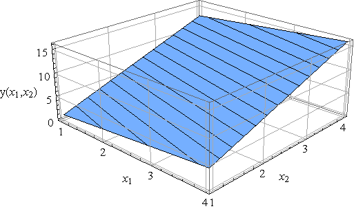
  Equation (1) can be interpreted as the equation of a plane in three-dimensional space with coordinates $(x_{1},x_{2},y)$ in the domain restricted by values of $X_{1}$ and $X_{2}$. This plane can also be determined by the equation $(\vec{n},\vec{r}-\vec{r_{0}})=0$, where the vector $\vec{n}$ is a normal to the plane, and the vector $\vec{r}-\vec{r_{0}}$ is an arbitrary vector on the plane.

  In Fig. 1, we present the example of the plane $y(x_{1},x_{2})$ with $X_{1}=X_{2}=4$ defined by the equation

  $$y=y(x_{1},x_{2})=x_{1}+(x_{2}-1)4,\qquad 1\leq x_{1},x_{2}\leq 4,$$

  or by the normal vector $\vec{n}=\{1,4,-1\}$ and vector $\vec{r_{0}}=\{1,1,1\}$. The domain $\{1\leq x_{1}\leq 4,~{}1\leq x_{2}\leq 4\}$ represents a parallelogram in three-dimensional space with coordinates $(x_{1},x_{2},y)$ with vertices in dots $\{1,1,1\},~{}\{1,4,5\},~{}\{4,1,12\}$, and $\{4,4,16\}$.

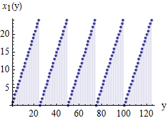
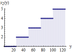
  In Figs. 2 and 3, we present the plots of functions $x_{1}(y)$ and $x_{2}(y)$ describing the bijective map (2) and (3).

  

  Figure 1: The plane $(\vec{n},\vec{r}-\vec{r_{0}})=0$ with domain $1\leq x_{1},~{}x_{2}\leq 4$, normal vector $\vec{n}=\{1,4,-1\}$, and vector $\vec{r_{0}}=\{1,1,1\}$.

  

  Figure 2: The coordinate $x_{1}$ versus the integer $y$; here $N=125$, $X_{1}=25$, and $X_{2}=5$.

  

  Figure 3: The coordinate $x_{2}$ versus the integer $y$; here $N=125$, $X_{1}=25$, and $X_{2}=5$.

• The bijective map for the set of integer numbers $y$ and the set of three integer variables $x_{1}$, $x_{2}$, and $x_{3}$ is described by functions $y(x_{1},x_{2},x_{3})$, $~{}x_{1}(y)$, $~{}x_{2}(y)$, and $x_{3}(y)$, where

  $$y=y(x_{1},x_{2},x_{3})=x_{1}+(x_{2}-1)X_{1}+(x_{3}-1)X_{1}X_{2},\quad 1\leq x_{i}\leq X_{i},~{}i\in[1,3].$$ (4)

  The function $x_{1}(y)$ is determined by the relation

  $$x_{1}(y)=y\mod{X_{1}}.$$ (5)

  The function $x_{2}(y)$ reads

  $$x_{2}(y)-1=\frac{y-x_{1}(y)}{X_{1}}\mod{X_{2}}.$$ (6)

  The function $x_{3}(y)$ is

  $$x_{3}(y)-1=\frac{y-x_{1}(y)-(x_{2}(y)-1)X_{1}}{X_{1}X_{2}}\mod{X_{3}}.$$ (7)

  The domain for functions $x_{1}(y)$, $x_{2}(y)$, and $x_{3}(y)$ is given as $1\leq y~{}\leq N$ in all three cases.

• The bijective map for the set of integer numbers $y$ and the set of $n$ integer variables $x_{i}$ reads

  $$y=y(x_{1},x_{2},\ldots,x_{n})=x_{1}+\sum_{k=2}^{n}(x_{k}-1)\prod_{j=1}^{k-1}X_{j},\qquad 1\leq x_{i}\leq X_{i},\quad i\in[1,n].$$ (8)

  The function $x_{k}(y)$ is

  $$x_{k}(y)-1=\frac{y-(x_{1}+\sum_{i=2}^{k}(x_{i}-1)\prod_{j=1}^{i-1}X_{j})}{\prod_{j=1}^{k}X_{j}}\mod{X_{k}},\qquad k=1,\ldots,n,\quad 1\leq y\leq N.$$ (9)

  For example, $x_{4}(y)=\dfrac{y-(x_{1}+(x_{2}-1)X_{1}+(x_{3}-1)X_{1}X_{2})}{X_{1}X_{2}X_{3}}\mod{X_{4}}$.

Equation (8) determines an $n$-dimensional plane in an ($n+1$)-dimensional space with coordinates $(x_{1},x_{2},\ldots,y)$. The other way to determine this plane is to use the equation

$$(\vec{n},\vec{r}-\vec{r_{0}})=0,\qquad\vec{n}=\{1,X_{1},X_{1}X_{2},\ldots,X_{1}\ldots\ldots\ldots X_{n-1},-1\};$$

$\vec{r_{0}}$ is the vector determining the position to any dot on the plane; for example, it may be the vector $\vec{r_{0}}=\{1,1,\ldots,1\}$.

Using the above formulas (8) and (9), we can find $y$ if we know $x_{1},x_{2},\ldots,x_{n}$; vice versa, if we know $y$, we can find every $x_{i}$, $i=1,\ldots,N$. In other words, we have the one-to-one correspondence between the set of integers $y$ and the set of integers $x_{i}$, and the map can be illustrated on an example of the above partition into two factors of number $N=X_{1}\times X_{2}=4\times 4$, where the integer number $y$ corresponds to the set of two integer numbers $x_{1}$ and $x_{2}$.

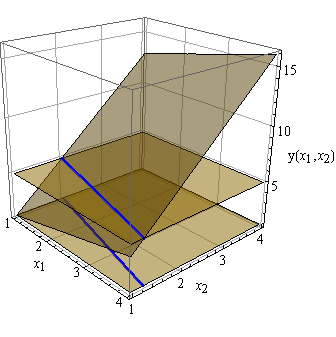
In Fig. 4, we illustrate the intersection between the plane $y(x_{1},x_{2})$ determined in Eqs. (1)–(3) and the plane $y=5$ or the intersection between the plane with normal vectors $\vec{n_{1}}=\{1,4,-1\}$, $\vec{n_{2}}=\{0,0,1\}$ and the common-position vector $\vec{r_{0}}=\{2,2,5\}$. This intersection is a line on which only one dot with both integer numbers $x_{1}$ and $x_{2}$ is located; in this case, according to (1)–(3), $x_{1}=2$ and $x_{2}=2$. This intersection is a line determined by the system of equations for the plane $y=5$ and the plane shown in Fig. 1 and determined by Eqs. (1)–(3). These equations for the particular example read

$$\begin{cases}&y-5=0,\\ &y-x_{1}-4(x_{2}-1)=0.\end{cases}$$ (10)

Also the intersection line is determined by the equation $[\vec{a},\vec{r}-\vec{r_{0}}]=\vec{0}$, where the vector $\vec{a}=[\vec{n_{1}},\vec{n_{2}}]=\{4,1,0\}$ and the vector $\vec{r_{0}}=\{2,2,5\}$ provide the position of the dot on the line.

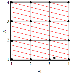
For every integer number $y^{\prime}$, we plot the intersection (line) of the plane $y=y^{\prime}$ with the plane $y(x_{1},x_{2})$ determined by (1)–(3) and then project the lines to the plane parallel to the plane $y=0$. Every such intersection corresponds to only one dot with integers $x_{1}$ and $x_{2}$ within the domain $x_{1}\in[1,X_{1}]$ and $x_{2}\in[1,X_{2}]$.

In the case presented, we have 16 intersections between the mentioned plane $y=y(x_{1},x_{2})$ and planes $y=y^{\prime}$ for every integer $y^{\prime}=1,\ldots,16$. Every intersection corresponds to one set of three integer numbers $y$, $x_{1}$, and $x_{2}$. These intersections, being projected into one plane, have the same angle $\alpha$, with $\tan\alpha=\dfrac{X_{2}-1}{X_{2}}\,\dfrac{1}{X_{1}}$. We show the projections in Fig. 5.

In $(n+1)$-dimensional space, the intersection of two planes with normal vectors $\vec{n_{1}}$ and $\vec{n_{2}}$ is a ($n-1$)-dimensional plane determined by the equation $[\vec{a},\vec{r}-\vec{r_{0}}]=\vec{0}$ with the vector $\vec{a}=[\vec{n_{1}},\vec{n_{2}}]$ and the position vector $\vec{r_{0}}$.

Figure 4: Intersection between the plane
$y(x_{1},x_{2})=x_{1}+4(x_{2}-1),~{}1\leq x_{1},x_{2}\leq 4$
and the plane $y=5$.

Figure 5: Projections of intersections between the plane $y(x_{1},x_{2})=x_{1}+4(x_{2}-1),~{}1\leq x_{1},x_{2}\leq 4$ and planes $y=y^{\prime}$, where $y^{\prime}=1,\ldots,16$.

3 Properties of the Shannon Entropy in Terms of the Probability p(y)

3.1 Subadditivity Condition

One of the main properties of the Shannon entropy for the joint probability distribution of a bipartite system $AB$ is the subadditivity condition, which reads

$$H(A)+H(B)\geq H(AB),$$ (11)

where $A$ and $B$ are the subsystems of the system $AB$. Below we consider coordinates $x_{1}$ and $x_{2}$ as discrete integer variables.

Let $p(x_{1},x_{2})$, where $1\leq x_{1}\leq X_{1}$, $~{}1\leq x_{2}\leq X_{2}$, be a joint probability distribution for a composite system $AB$ with finite number $N=X_{1}X_{2}$ of elements, $\mathcal{P}(x_{1})=\sum_{x_{2}=1}^{X_{2}}p(x_{1},x_{2})$ be the probability distribution for system $B$, and $\Pi=\sum_{x_{1}=1}^{X_{1}}p(x_{1},x_{2})$ be the probability distribution for system $A$. Now we can rewrite the subadditivity condition (11) as follows:

$$-\sum_{x_{1}=1}^{X_{1}}\mathcal{P}(x_{1})\log\mathcal{P}(x_{1})-\sum_{x_{2}=1}^{X_{2}}\Pi(x_{2})\log\Pi(x_{2})\geq-\sum_{x_{1}=1}^{X_{1}}\sum_{x_{2}=1}^{X_{2}}p(x_{1},x_{2})\log p(x_{1},x_{2}).$$ (12)

The transition from the probability distribution $p(x_{1},x_{2})$, $1\leq x_{1}\leq X_{1}$, $~{}1\leq x_{2}\leq X_{2}$ depending on two integer variables to the probability distribution $f(y)$, $1\leq y\leq N$ depending on one integer variable $y$ can be performed using the bijective map (1); we have the probability distribution of the indivisible system

$$f\big{(}y(x_{1},x_{2})\big{)}=p(x_{1},x_{2}).$$ (13)

The two marginal probability distributions read

$$\mathcal{P}(x_{1})=\sum_{x_{2}=1}^{X_{2}}p(x_{1},x_{2})=\sum_{x_{2}=1}^{X_{2}}f(y(x_{1},x_{2}))=\sum_{x_{2}=1}^{X_{2}}f(x_{1}+(x_{2}-1)X_{1})$$ (14)

and

$$\Pi(x_{2})=\sum_{x_{1}=1}^{X_{1}}p(x_{1},x_{2})=\sum_{x_{1}=1}^{X_{1}}f(y(x_{1},x_{2}))=\sum_{x_{1}=1}^{X_{1}}f(x_{1}+(x_{2}-1)X_{1}).$$ (15)

This transition provides the possibility to rewrite inequality (12) in the form

$$-\sum_{x_{1}=1}^{X_{1}}\left(\sum_{x_{2}=1}^{X_{2}}f(x_{1}+(x_{2}-1)X_{1})\log\sum_{x_{2}=1}^{X_{2}}f(x_{1}+(x_{2}-1)X_{1})\right)$$

$$-\sum_{x_{2}=1}^{X_{2}}\left(\sum_{x_{1}=1}^{X_{1}}f(x_{1}+(x_{2}-1)X_{1})\log\sum_{x_{1}=1}^{X_{1}}f(x_{1}+(x_{2}-1)X_{1})\right)\geq-\sum_{y=1}^{N}f(y)\log f(y).$$ (16)

Inequality (16) is the main result of our consideration of a set of nonnegative numbers $p(y)=\dfrac{|s_{y}|}{\sum_{y^{\prime}=1}^{N}|s_{y^{\prime}}|}$ associated with real numbers $s_{y}$. Such set $p(y)$, considered as the probability distribution and denoted in this case as $f(y)$, always satisfies the obtained inequality (16).

The difference between the left-hand side and the right-hand side of inequality (16) gives the Shannon information $I=H(A)+H(B)-H(AB)\geq 0$, or joint information, which takes only nonnegative values.

3.2 Entropy of the Composite System

The Shannon entropy of a composite system with subsystems $A_{1}A_{2}\ldots A_{n}$ satisfies the equality

$$H(A_{1}A_{2}\ldots A_{n})=H(A_{1})+H(A_{2}|A_{1})+\cdots+H(A_{n}|A_{1},A_{2},\ldots,A_{n-1}).$$ (17)

Here, the Shannon entropy of the conditional probability distribution $Q(x_{1}|x_{2})=\dfrac{p(x_{1},x_{2})}{\Pi(x_{2})}$ is

$$H(A|B)=H(Q(x_{1}|x_{2}))=-\sum_{x_{1}=1}^{X_{2}}\sum_{x_{2}=1}^{X_{1}}p(x_{1},x_{2})\log Q(x_{1},x_{2}).$$

In the case of composite system $AB$, expression (17) reduces to the form

$$H(AB)=H(B)+H(A|B)\qquad\mbox{or}\qquad H(p(x_{1},x_{2}))=H(\Pi(x_{2}))+H(Q(x_{1}|x_{2})).$$ (18)

Using the bijective map described by Eqs. (1)–(3), we present Eq. (18) in terms of the function $f(y)$ as follows:

$$-\sum_{y=1}^{X_{1}\cdot X_{2}}f(y)\log а(y) = -\sum_{x_{2}=1}^{X_{2}}\sum_{x_{1}=1}^{X_{1}}f(x_{1}+(x_{2}-1)X_{1})\log\sum_{x_{1}=1}^{X_{1}}f(x_{1}+(x_{2}-1)X_{1})$$ (19)

$$-\sum_{x_{1}=1}^{X_{2}}\sum_{x_{2}=1}^{X_{1}}f(x_{1}+(x_{2}-1)X_{1})\log\frac{f(x_{1}+(x_{2}-1)X_{1})}{\sum_{x_{1}=1}^{X_{1}}f(x_{1}+(x_{2}-1)X_{1})},$$

where $f(y)$ is the probability distribution of one random variable $1\leq y\leq N$. Here, the integers $x_{1}$ and $x_{2}$ belong to domain $1\leq x_{1}\leq X_{1}$ and $1\leq x_{2}\leq X_{2}$.

4 Entropic Inequalities for Clebsch–Gordan Coefficients

The Clebsch–Gordan coefficients $\left<j_{1}m_{1}j_{2}m_{2}\vphantom{jm}\right|\left.jm\vphantom{j_{1}m_{1}j_{2}m_{2}}\right>$ are defined as follows [13]:

$$\psi_{jm}=\sum_{m_{1},m_{2}}\left<j_{1}m_{1}j_{2}m_{2}\vphantom{jm}\right|\left.jm\vphantom{j_{1}m_{1}j_{2}m_{2}}\right>\psi_{j_{1}m_{1}}^{(1)}\psi_{j_{2}m_{2}}^{(2)},\qquad m=m_{1}+m_{2},$$ (20)

where $\psi_{jm}$ is the wave function of the spin system with spin $j$ and the spin projection $m$, and $\psi_{j_{1}m_{1}}^{(1)}$ and $\psi_{j_{2}m_{2}}^{(2)}$ are two wave functions of the spin system with spin $j_{1}$ and the spin projection $m_{1}$ and spin $j_{2}$ and the spin projection $m_{2}$, respectively.

4.1 Subadditivity Inequality

We can express the Clebsch–Gordan coefficients as functions of integer variable $y=1,\ldots,N$, where $N=(2j_{1}+1)(2j_{2}+1)$, using the relation $m_{i}=x_{i}-j_{i}-1$, $i=1,2$ and the relation between $x_{i}$ and $y$ given by (1)–(3). We employ the partition $N=X_{1}\times X_{2}$, where $X_{i}=2j_{i}+1$ ($i=1,2$).

We adopt the approach [4] and apply it to the squares of the Clebsch–Gordan coefficients $\left<m_{1},m_{2}\vphantom{jm}\right|\left.jm\vphantom{m_{1},m_{2}}\right>$ as the probabilities

$$p(m_{1},m_{2})=|\left<m_{1},m_{2}\vphantom{jm}\right|\left.jm\vphantom{m_{1},m_{2}}\right>|^{2}=f(y(m_{1},m_{2})).$$ (21)

In the formulas below, we omit arguments $j$ and $m$ in the definition of probabilities connected with the Clebsch–Gordan coefficients, since for such the probabilities the values of $j$ and $m$ are fixed.

In view of (1)–(3), we obtain the functions $m_{1}(y)$ and $m_{2}(y)$ as follows:

$$m_{1}(y)=[y\mod(2j_{1}+1)]-j_{1}-1,\qquad m_{2}(y)=\left[\frac{y-[y\mod(2j_{1}+1)]}{2j_{1}+1}\mod(2j_{2}+1)\right]-j_{2}.$$

We introduce the probability mentioned above in terms of the integer number $y$; it reads

$$f(y)=\left|\left<[y\mod(2j_{1}+1)]-1-j_{1},\left[\frac{y-[y\mod(2j_{1}+1)]}{2j_{1}+1}\mod{(2j_{2}+1)}\right]-j_{2}\vphantom{jm}\right|\left.jm\vphantom{[y\mod(2j_{1}+1)]-1-j_{1},\left[\frac{y-[y\mod(2j_{1}+1)]}{2j_{1}+1}\mod{(2j_{2}+1)}\right]-j_{2}}\right>\right|^{2}.$$ (22)

In [4], we derived the subadditivity condition (11) for the Shannon entropy in terms of the Clebsch–Gordan coefficients, which reads

$$-\sum_{m_{2}=-j_{2}}^{j_{2}}|\left<j_{1}m_{1}j_{2}m_{2}\vphantom{jm}\right|\left.jm\vphantom{j_{1}m_{1}j_{2}m_{2}}\right>|^{2}\log\left[\sum_{m_{2}=-j_{2}}^{j_{2}}|\left<j_{1}m_{1}j_{2}m_{2}\vphantom{jm}\right|\left.jm\vphantom{j_{1}m_{1}j_{2}m_{2}}\right>|^{2}\right]$$

$$-\sum_{m_{1}=-j_{1}}^{j_{1}}|\left<j_{1}m_{1}j_{2}m_{2}\vphantom{jm}\right|\left.jm\vphantom{j_{1}m_{1}j_{2}m_{2}}\right>|^{2}\log\left[\sum_{m_{1}=-j_{1}}^{j_{1}}|\left<j_{1}m_{1}j_{2}m_{2}\vphantom{jm}\right|\left.jm\vphantom{j_{1}m_{1}j_{2}m_{2}}\right>|^{2}\right]$$

$$\geq-\sum_{m_{1}=-j_{1}}^{j_{1}}\sum_{m_{2}=-j_{2}}^{j_{2}}|\left<j_{1}m_{1}j_{2}m_{2}\vphantom{jm}\right|\left.jm\vphantom{j_{1}m_{1}j_{2}m_{2}}\right>|^{2}\log\left[\sum_{m_{1}=-j_{1}}^{j_{1}}\sum_{m_{2}=-j_{2}}^{j_{2}}|\left<j_{1}m_{1}j_{2}m_{2}\vphantom{jm}\right|\left.jm\vphantom{j_{1}m_{1}j_{2}m_{2}}\right>|^{2}\right].$$ (23)

This inequality is a new entropic inequality for the Clebsch–Gordan coefficients.

After combining expressions (22) and (23), we arrive at the subadditivity condition [14, 15] in terms of a single variable $y$,

$$-\sum_{m_{2}=-j_{2}}^{j_{2}}f(y(m_{1},m_{2}))\log\sum_{m_{2}=-j_{2}}^{j_{2}}f(y(m_{1},m_{2}))-\sum_{m_{1}=-j_{1}}^{j_{1}}f(y(m_{1},m_{2}))\log\sum_{m_{1}=-j_{1}}^{j_{1}}f(y(m_{1},m_{2}))$$

$$\geq-\sum_{y=0}^{N}f(y(m_{1},m_{2}))\log\sum_{y=0}^{N}f(y(m_{1},m_{2})).$$ (24)

4.2 Strong Subadditivity Condition

The strong subadditivity property for Shannon entropy states that the conditional information for tripartite system $ABC$ takes nonnegative values and reads

$$H(ABC)+H(B)\geq H(AB)+H(BC).$$ (25)

In view of the one-to-one correspondence between the integer variable $y$ and a pair of integer variables $(x_{1},x_{2})$ and between $y$ and a triple of integer variables $(t_{1},t_{2},t_{3})$, i.e., using formulas (1)–(3) and (4)–(7), we can construct a bijective map between $(x_{1},x_{2})$ and $(t_{1},t_{2},t_{3})$. This means that we can write the strong subadditivity condition for the quantum system of two spins; it is

$$x_{1}(t_{1},t_{2},t_{3})=y\mod{X_{1}}=\big{[}(t_{3}-1)T_{2}T_{1}+(t_{2}-1)T_{1}+t_{1}\big{]}\mod{X_{1}},$$

$$x_{2}(t_{1},t_{2},t_{3})-1=\frac{y-x_{1}}{X_{1}}\mod{X_{2}}=\frac{\big{[}(t_{3}-1)T_{2}T_{1}+(t_{2}-1)T_{1}+t_{1}\big{]}-x_{1}}{X_{1}}\mod{X_{2}},$$

with the domain $1\leq t_{i}\leq T_{i}$, $~{}i=1,2,3$ for functions $x_{1}(t_{1},t_{2},t_{3})$ and $x_{2}(t_{1},t_{2},t_{3})$.

Now we are in the position to rewrite the squares of the Clebsch–Gordan coefficients as a probability distribution $g$ depending on three integer variables $(t_{1},t_{2},t_{3})$, which take values $N=T_{1}T_{2}T_{3}$, $~{}1\leq t_{i}\leq T_{i}$, $~{}i=1,2,3$ instead of two indices $m_{1}$ and $m_{2}$; it is

Combining the strong subadditivity (25) and the expression for Clebsch–Gordan coefficients as probability distributions $f(y)$ and $g(t_{1},t_{2},t_{3})$ (4.2), we obtain the following inequality:

$$-\sum_{y=1}^{N}f(y)\log f(y)-\sum_{t_{2}=1}^{T_{2}}\left(\sum_{t_{1}=1}^{T_{1}}\sum_{t_{3}=1}^{T_{3}}g(t_{1},t_{2},t_{3})\log\sum_{t_{1}=1}^{T_{1}}\sum_{t_{3}=1}^{T_{3}}g(t_{1},t_{2},t_{3})\right)\\ \geq-\sum_{t_{1}=1}^{T_{1}}\sum_{t_{2}=1}^{T_{2}}\left(\sum_{t_{3}=1}^{T_{3}}g(t_{1},t_{2},t_{3})\log\sum_{t_{3}=1}^{T_{3}}g(t_{1},t_{2},t_{3})\right)-\sum_{t_{2}=1}^{T_{2}}\sum_{t_{3}=1}^{T_{3}}\left(\sum_{t_{1}=1}^{T_{1}}g(t_{1},t_{2},t_{3})\log\sum_{t_{1}=1}^{T_{1}}g(t_{1},t_{2},t_{3})\right).$$ (27)

This inequality is a new relation for the Clebsch–Gordan coefficients.

5 Conclusions

We obtained functions (8) and (9) for the bijective map between the sequence of integer numbers and the sequence of sets of $n$ integer numbers and called them the function detecting the hidden correlations. These functions give a simple technique to consider any indivisible system consisting of a finite number of $N$ elements with probabilities as a system consisting of $n$ subsystems; this fact allows us to apply the properties of multipartite systems to indivisible systems. We employed this technique to obtain the properties of the Shannon entropy for probabilities associated with distributions, such as the subadditivity and strong subadditivity conditions for a single indivisible system.

The technique elaborated can be applied to any set of real numbers, which we associate with a set of probabilities according to the formula $p(y)=\dfrac{|s_{y}|}{\sum_{y^{\prime}=1}^{N}|s_{y^{\prime}}|}$, where $p(y)$ is the probability associated with a real number $s_{y}$, and $y$ takes integer values from $1$ to the number $N$ of elements in the set of considered real numbers. We also applied the new technique to obtain new entropic inequalities for the Clebsch–Gordan coefficients, which were considered as probability distributions of one random variable.

For an arbitrary $N$$\times$$N$ matrix $A$, there exists the matrix $\rho=\dfrac{A^{\dagger}A}{\mbox{Tr}\,{A^{\dagger}A}}$ with the properties of the density matrix, i.e., $\rho^{\dagger}=\rho$, Tr$\,\rho=1$, and $\rho\geq 0$. Using the entropic-information inequalities known for density matrices, one can obtain the corresponding inequalities for arbitrary $N$$\times$$N$ matrices $A$.

The results obtained in this work for real numbers and probability distributions will be extended in a future publication to the properties of arbitrary matrices. The entropic-information inequalities obtained can be applied [18, 16, 17] in experiments with superconducting qudits [21, 20, 19] based on the Josephson junction discussed in [23, 22]. The obtained explicit formulas of the introduced functions can be used to discuss the properties of quantum correlations like the violation of Bell inequalities [24], contextuality problems [25, 26], entanglement criteria [28, 27], and other correlations discussed in [29, 30] for different systems. Also it is worth noting that functions (1)–(3) in different notation were presented in the PhD Thesis [31] and employed in [32].

In the future publication, we relate the introduced formalism to the star-product quantization scheme discussed, e.g., in [33, 34] and study a possibility to introduce and employ the notion of “hidden states” for single qudit states (see [35]) extending the notion of gates for composite systems to the case of noncomposite systems.

References

• [1] M. A. Man’ko and V. I. Man’ko, J. Russ. Laser Res., 34, 203 (2013).
• [2] M. A Man’ko, V. I. Man’ko, G. Marmo, et al., Nuovo Cim. C, 36, 163 (2013).
• [3] V. I. Man’ko and L. A. Markovich, “Entropic inequalities for matrix elements of rotation group irreducible representations,” arXiv:quant-ph/1511.07341.
• [4] V. N. Chernega, O. V. Man’ko, V. I. Man’ko, and Z. Seilov, “New information and entropic inequalities for Clebsch–Gordan coefficients,” arXiv:quant-ph/1606.00854; Theor. Math. Phys. (2017, in press).
• [5] M. A. Man’ko and V. I. Man’ko, J. Russ. Laser Res., 36, 301 (2015).
• [6] M. A. Man’ko and V. I. Man’ko, Entropy, 37, 1 (2016).
• [7] M. A. Man’ko and V. I. Man’ko, J. Phys.: Conf. Ser., 698, 012004 (2016).
• [8] V. N. Chernega and O. V. Man’ko, Phys. Scr., 90, 074052 (2015).
• [9] A. S. Holevo, Probabilistic and Statistical Aspects of Quantum Theory, North Holland, Amsterdam (1982).
• [10] W. Feller, An Introduction to Probability Theory and its Applications, Wiley (1957), Vol. 1.
• [11] A. N. Kolmogorov, Foundations of the Theory of Probability, Chelsea Publishing Company, New York (1956).
• [12] A. N. Shiryaev, Probability, Springer (1996).
• [13] L. D. Landau and E. M. Lifshitz, Quantum Mechanics: Non-Relativistic Theory. Butterworth-Heinemann, Oxford (1977).
• [14] E. H. Lieb and M. B. Ruskai, J. Math. Phys., 14, 1938 (1973).
• [15] M. A. Nielsen and D. A. Petz, “A simple proof of the strong subadditivity inequality,” arXiv:quant-ph/0408130 (2004).
• [16] A. K. Fedorov, E. O. Kiktenko, O. V. Man’ko, and V. I. Man’ko, Phys. Rev. A, 91, 042312 (2015).
• [17] E. O. Kiktenko, A. K. Fedorov, A. A. Strakhov, and V. I. Man’ko, Phys. Lett. A, 379, 1409 (2015).
• [18] E. Glushkov, A. Glushkova, and V. I. Man’ko, J. Russ. Laser Res., 36, 448 (2015).
• [19] M. H. Devoret and R. J. Schoelkopf, Science, 339, 1169 (2013).
• [20] Y. A. Pashkin, T. Yamamoto, O. Astafiev, et al., Nature, 421, 823 (2003).
• [21] Y. Shalibo, R. Resh, O. Fogel, et al., Phys. Rev. Lett., 110, 100404 (2013).
• [22] T. Fujii, S. Matsuo, N. Hatakenaka, et al., Phys. Rev. B, 84, 174521 (2011).
• [23] V. V. Dodonov, V. I. Man’ko, and O. V. Man’ko, J. Sov. Laser Res., 10, 413 (1989).
• [24] J. S. Bell, Physica, 1, 195 (1964).
• [25] A. A. Klyachko, H. Ali Can, S. Binicioglu, and A. S. Shumovsky, Phys. Rev. Lett., 101, 020403 (2008).
• [26] A. E. Rastegin, “Tests for quantum contextuality in terms of q𝑞q-entropies,” arXiv:quant-ph/1210.6742.
• [27] P. Horodecki, R. Horodecki, and M. Horodecki, Phys. Lett. A, 223, 1 (1996).
• [28] A. Peres, Phys. Rev. Lett., 77, 1413 (1996).
• [29] D. Petz, J. Phys. A: Math. Gen., 35, 929 (2002).
• [30] I. Bengtsson and K. Zyczkowski, Geometry of Quantum States: An Introduction to Quantum Entanglement, Cambridge University Press (2008).
• [31] A. De Pasquale, “Bipartite entanglement of large quantum systems,” arXiv:quant-ph/1206.6749.
• [32] A. De Pasquale, P. Facchi. V. Giovannetti, et al., J. Phys. A: Math. Theor., 45, 015308 (2012).
• [33] O. V. Man’ko, V. I. Marmo, G. Marmo, and P. Vitale, Phys. Lett. A, 360, 522 (2007).
• [34] L. Rosa and P. Vitale, Mod. Phys. Lett. A, 27, 1250207 (2012).
• [35] A. A. Popov, E. O. Kiktanko, A. K. Fedorov, and V. I. Man’ko, J. Russ. Laser Res., 37, 581 (2016).