The VIMOS Public Extragalactic Redshift Survey (VIPERS)

We carry out a joint analysis of redshift-space distortions and galaxy-galaxy lensing, with the aim of measuring the growth rate of structure; this is a key quantity for understanding the nature of gravity on cosmological scales and late-time cosmic acceleration. We make use of the final VIPERS redshift survey dataset, which maps a portion of the Universe at a redshift of $z\simeq 0.8$, and the lensing data from the CFHTLenS survey over the same area of the sky. We build a consistent theoretical model that combines non-linear galaxy biasing and redshift-space distortion models, and confront it with observations. The two probes are combined in a Bayesian maximum likelihood analysis to determine the growth rate of structure at two redshifts $z=0.6$ and $z=0.86$. We obtain measurements of $f\sigma_{8}(0.6)=0.48\pm 0.12$ and $f\sigma_{8}(0.86)=0.48\pm 0.10$. The additional galaxy-galaxy lensing constraint alleviates galaxy bias and $\sigma_{8}$ degeneracies, providing direct measurements of $f$ and $\sigma_{8}$: $\left[f(0.6),\sigma_{8}(0.6)\right]=[0.93\pm 0.22,0.52\pm 0.06]$ and $\left[f(0.86),\sigma_{8}(0.86)\right]=[0.99\pm 0.19,0.48\pm 0.04]$. These measurements are statistically consistent with a Universe where the gravitational interactions can be described by General Relativity, although they are not yet accurate enough to rule out some commonly considered alternatives. Finally, as a complementary test we measure the gravitational slip parameter, $E_{G}$, for the first time at $z>0.6$. We find values of $\smash{\overline{E}_{G}}(0.6)=0.16\pm 0.09$ and $\smash{\overline{E}_{G}}(0.86)=0.09\pm 0.07$, when $E_{G}$ is averaged over scales above $3\,h^{-1}\leavevmode\nobreak\ {\rm Mpc}$. We find that our $E_{G}$ measurements exhibit slightly lower values than expected for standard relativistic gravity in a $\Lambda\rm{CDM}$ background, although the results are consistent within $1-2\sigma$.

1 Introduction

The origin of the late-time acceleration of the universal expansion is a major question in cosmology. The source of this acceleration and its associated energy density are crucial in understanding the properties of the Universe and its evolution and fate. In the standard cosmological model, this cosmic acceleration can be associated with the presence of a dark energy component, a cosmological fluid with negative pressure, which opposes the gravitational force on large scales. However, this apparent acceleration can conversely be interpreted as a failure of the standard relativistic theory of gravity. A key goal for cosmology is therefore to investigate the nature of gravity empirically. To be clear, what can potentially be falsified is the validity of Einstein’s field equations, rather than General Relativity itself; this sets a broader framework within which Einstein gravity or modified alternatives can operate.

The large-scale structure of the Universe has proved to be very powerful for testing the cosmological model through the use of various observables such as the two-point statistics of the galaxy distribution and its features (e.g. Peacock et al. 2001; Cole et al. 2005; Tegmark et al. 2004; Eisenstein et al. 2005; Guzzo et al. 2008; Percival et al. 2010; Beutler et al. 2011; Blake et al. 2012; Anderson et al. 2014; Alam et al. 2017, and references therein). In this context, a unique probe of gravitational physics is the large-scale component of galaxy peculiar velocities affecting the observed galaxy distribution in redshift surveys (Guzzo et al. 2008), sensitive to the growth rate of structure $f$ defined as $\mathrm{d}\ln D/\mathrm{d}\ln a$, where $D$ and $a$ are respectively the linear growth factor and scale factor. In turn, the growth rate of structure tells us about the strength of gravity acting on cosmological scales and is a direct prediction of gravity theories. The distortions induced by peculiar velocities in the apparent galaxy clustering, the so-called redshift-space distortions (RSD), are a very important cosmological probe of the nature of gravity. In the last decade, they have been studied in large galaxy redshift surveys, showing a broad consistency with $\Lambda\rm{CDM}$ and General Relativity predictions (e.g. Blake et al. 2012; Beutler et al. 2012; de la Torre et al. 2013; Samushia et al. 2014; Gil-Marín et al. 2016; Chuang et al. 2016).

Although galaxy redshift surveys are powerful cosmological tools for understanding the geometry and the dynamics of the Universe, they are fundamentally limited by the inherent uncertainty related to the bias of galaxies, the fact that these are not faithful tracers of the underlying matter distribution. Gravitational lensing represents a powerful probe that is complementary to galaxy redshift-space clustering. In the weak regime in particular, the statistical shape deformations of background galaxies probe the relativistic gravitational deflection of light by the projected dark matter fluctuations due to foreground large-scale structure. There are several techniques associated with weak gravitational lensing; one that is particularly useful for combining with galaxy clustering is galaxy-galaxy lensing. This technique consists of studying the weak deformations of background galaxies around foreground galaxies, whose associated dark matter component acts as a gravitational lens. This is particularly useful for probing the galaxy-matter cross-correlation, which in turn provides insights on the bias of foreground galaxies and the matter energy density $\Omega_{m}$, although the projected nature of the statistic makes it insensitive to redshift-space distortions. The combination of galaxy-galaxy lensing with redshift-space galaxy correlations is therefore a very promising way to study gravitational physics, given that both lensing information on background sources and spectroscopic information on foreground galaxies are available on the same field.

Beyond the determination of the growth rate of structure, one can define consistency tests of gravity that are sensitive to both the Newtonian and curvature gravitational potentials, $\Psi$ and $\Phi$ respectively (e.g. Simpson et al. 2013). One is the gravitational slip, $E_{G}$, which was originally proposed by Zhang et al. (2007) and implemented by Reyes et al. (2010) in terms of the ratio between the galaxy-galaxy lensing signal and the redshift-space distortions parameter $\beta=f/b$ times the galaxy clustering signal of the lenses. Here $b$ is the galaxy linear bias. $E_{G}$ effectively tests whether the Laplacian of $\Psi+\Phi$, to which gravitational lensing is sensitive, and that of $\Psi$, to which galaxy peculiar velocities are sensitive, are consistent with standard gravity predictions. In the standard cosmological model, $E_{G}$ asymptotes to $\Omega_{m}/f$ on large linear scales. A failure of this test would either imply an incorrect matter energy density or a departure from standard gravity. This test has been performed at low redshift in the SDSS survey by Reyes et al. (2010) and more recently at redshifts up to $z=0.57$ by Blake et al. (2016) and Pullen et al. (2016).

The $E_{G}$ statistic is formally defined as $E_{G}=\Upsilon_{gm}/(\beta\Upsilon_{gg})$, where $\Upsilon_{gm}$ and $\Upsilon_{gg}$ are filtered versions of the real-space projected galaxy-matter and galaxy-galaxy correlation functions respectively, and $\beta$ is the RSD parameter. In practice, its implementation involves measuring $\beta$ and the ratio $\Upsilon_{gm}/\Upsilon_{gg}$ separately, to finally combine them. But since $\beta$ and $\Upsilon_{gg}$ are extracted from the same observable, namely the anisotropic two-point correlation function of lens galaxies, this is suboptimal and does not account for the covariance between them. In this analysis, we follow a different approach. We combine the galaxy-galaxy lensing quantity $\Upsilon_{gm}$ and the redshift-space anisotropic correlation function monopole and quadrupole moments $\xi_{0}$ and $\xi_{2}$ (from which $\beta$ can be estimated) in a joint likelihood analysis, to provide constraints on $f$ and gravity at redshifts above $z=0.6$. We note that we do not include $\Upsilon_{gg}$ because of the redundant cosmological information shared with $\xi_{0}$ and $\xi_{2}$.

The VIMOS Public Extragalactic Redshift Survey (VIPERS) is a large galaxy redshift survey probing the $z\simeq 0.8$ Universe with an unprecedented density of spectroscopic galaxies of $5\times 10^{-3}\,h^{3}\leavevmode\nobreak\ {\rm Mpc^{-3}}$ and covering an overall area of $23.5\leavevmode\nobreak\ \rm{deg}^{2}$ on the sky. The prime goal of VIPERS is an accurate measurement of the growth rate of structure at redshift around unity. A first measurement has been performed using the Public Data Release 1 (PDR-1), setting a reference measurement of $f\sigma_{8}$ at $z=0.8$ (de la Torre et al. 2013). The survey is now complete and several analyses including this one are using the final dataset to produce the VIPERS definitive growth rate of structure measurements, but following a variety of approaches. The present analysis aims at maximizing the cosmological information available and takes advantage of the overlapping lensing information provided by CFHTLenS lensing survey, to provide a precise gravity test at redshifts $0.5<z<1.2$ by combining RSD and galaxy-galaxy lensing.

The paper is organized as follows. The data are described in Sect. 2; Sect. 3 describes our methods for estimating galaxy clustering and galaxy-galaxy lensing; Sect. 4 describes the theoretical modelling that is tested in Sect. 5; Sect. 6 presents how the likelihood analysis is constructed; Sect. 7 describes the cosmological results, and Sect. 8 summarizes our findings and concludes.

Throughout this analysis and if not stated otherwise, we assume a flat $\Lambda{\rm CDM}$ ($\Lambda$-Cold Dark Matter) cosmological model with $(\Omega_{m},\Omega_{b},n_{s})=(0.3,0.045,0.96)$ and a Hubble constant of $H_{0}=100\leavevmode\nobreak\ h\leavevmode\nobreak\ \rm{km\leavevmode\nobreak\ s^{-1}\leavevmode\nobreak\ Mpc^{-1}}$.

2 Data

2.1 Combined VIPERS-CFHTLenS dataset

The VIPERS galaxy target sample was selected from the optical photometric catalogues of the Canada-France-Hawaii Telescope Legacy Survey Wide (CFHTLS-Wide, Goranova et al. 2009). VIPERS covers $23.5$ deg² on the sky, divided over two areas within the W1 and W4 CFHTLS fields. Galaxies are selected to a limit of $i_{\rm AB}<22.5$, applying a simple and robust $gri$ colour pre-selection to efficiently remove galaxies at $z<0.5$. Coupled with a highly optimized observing strategy (Scodeggio et al. 2009), this allows us to double the galaxy sampling rate in the redshift range of interest, with respect to a pure magnitude-limited sample. At the same time, the area and depth of the survey result in a relatively large volume, $5\times 10^{7}\,h^{-3}\leavevmode\nobreak\ {\rm Mpc^{3}}$, analogous to that of the Two Degree Field Galaxy Redshift Survey (2dFGRS) at $z\simeq 0.1$ (Colless et al. 2001, 2003). Such a combination of sampling rate and depth is unique amongst current redshift surveys at $z>0.5$. VIPERS spectra are collected with the VIMOS multi-object spectrograph (Le Fèvre et al. 2003) at moderate resolution ($R=220$) using the LR Red grism, providing a wavelength coverage of 5500-9500$\rm{\AA}$ and a redshift error corresponding to a galaxy peculiar velocity error at any redshift of $\sigma_{\rm vel}=163$$\,{\rm km\,s^{-1}}$. The full VIPERS area of $23.5$ deg² is covered through a mosaic of 288 VIMOS pointings (192 in the W1 area, and 96 in the W4 area). A discussion of the survey data reduction and management infrastructure is presented in Garilli et al. (2014). A complete description of the survey construction, from the definition of the target sample to the actual spectra and redshift measurements, is given in the survey description paper (Guzzo et al. 2014).

The data used here correspond to the publicly released PDR-2 catalogue (Scodeggio et al. 2017) that includes $86\,775$ galaxy spectra, with the exception of a small sub-set of redshifts (340 galaxies missing in the range $0.6<z<1.1$), for which the redshift and quality flags were revised closer to the release date. Concerning the analysis presented here, this has no effect. A quality flag has been assigned to each object in the process of determining their redshift from the spectrum, which quantifies the reliability of the measured redshifts. In this analysis (as with all statistical analyses presented in the parallel papers of the final science release), we use only galaxies with flags 2 to 9 inclusive, corresponding to objects with a redshift confidence level of $96.1\%$ or larger. This has been estimated from repeated spectroscopic observations in the VIPERS fields (see Scodeggio et al. 2017). The catalogue used here, which we will refer to just as the VIPERS sample in the following, includes $76584$ galaxies with reliable redshift measurements.

In addition to the VIPERS spectroscopic sample, we make use of the public lensing data from the Canada-France-Hawaii Lensing Survey (Heymans et al. 2012), hereafter referred to as CFHTLenS. The CFHTLenS survey analysis combined weak lensing data processing with theli (Erben et al. 2013), shear measurement with lensfit (Miller et al. 2013), and photometric redshift measurement with PSF-matched photometry (Hildebrandt et al. 2012). A full systematic error analysis of the shear measurements in combination with the photometric redshifts is presented in Heymans et al. (2012), with additional error analyses of the photometric redshift measurements presented in Benjamin et al. (2013).

2.2 Sample selection

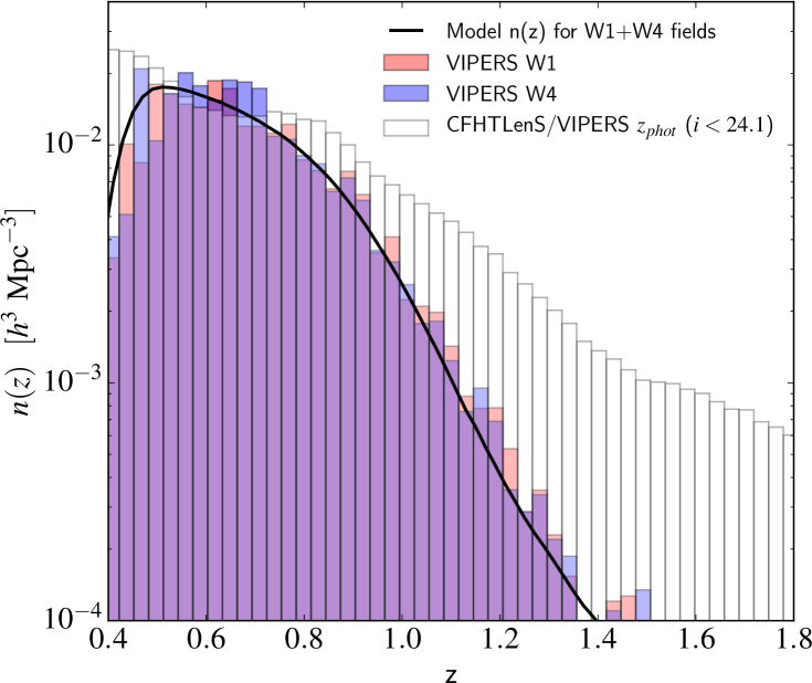
For this analysis, we define two redshift intervals covering the full volume of the VIPERS survey: $0.5<z<0.7$ and $0.7<z<1.2$. The number density of galaxies in the combined W1 and W4 fields is presented in Fig. 1, after correction with survey incompleteness weights $w^{C}$ (see Sect. 3.1). It is worth emphasizing that after application of survey incompleteness corrections, the VIPERS spectroscopic sample represents a statistically unbiased subset of the parent $i_{\rm AB}<22.5$ photometric catalogue (Guzzo et al. 2014; Garilli et al. 2014; Scodeggio et al. 2017). The redshift distribution is modelled using the $V_{\rm max}$ method (Cole 2011; de la Torre et al. 2013) and shown with the solid curve in the figure. In this method, we randomly sample 500 times the $V_{\rm max}$ of each galaxy, defined as the comoving volume between the minimum and maximum redshifts where the galaxy is observable given its apparent magnitude and the magnitude limit of VIPERS, $i_{\rm AB}=22.5$. The redshift distribution thus obtained is regular and can be straightforwardly interpolated with a smooth function, showed with the solid curve in Fig. 1.

In addition to VIPERS spectroscopic galaxies, photometric galaxies from the CFHTLenS survey on the overlapping areas with VIPERS survey, have been used for the galaxy-galaxy lensing. The lens sample satisfies the VIPERS selection $i_{\rm AB}<22.5$ and uses VIPERS spectroscopic redshifts when available (i.e. for about $30\%$ of objects) or CFHTLenS maximum likelihood photometric redshifts otherwise. The sources have been selected to have $i_{\rm AB}<24.1$ and thus have a higher surface density. Sources inside the mask delimiting bad photometric areas in the CFHTLenS catalogue have been discarded. We also make use of the individual source redshift probability distribution function estimates obtained from bpz (Hildebrandt et al. 2012) as described in Sect. 3.2. Source galaxies extend above $z_{\rm phot}=1.4$ and their number density is represented with the unfilled histogram in Fig. 1.

Figure 1: Number densities of VIPERS galaxies in the individual W1 and W4 fields and of CFHTLenS/VIPERS photometric redshift galaxies, as a function of redshift. The number densities of VIPERS galaxies are corrected for the survey incompleteness by weighting each galaxy in the counts by its associated inverse completeness weight $w^{C}$. The solid curve corresponds to the model $n(z)$ used in the analysis. It was obtained by randomly sampling galaxy redshifts within their $V_{\rm max}$ (see text for details).

3 Galaxy clustering and galaxy-galaxy lensing estimation

3.1 Anisotropic galaxy clustering estimation

We estimate the redshift-space galaxy clustering by measuring the two-point statistics of the spatial distribution of galaxies in configuration space. For this we infer the anisotropic two-point correlation function $\xi(s,\mu)$ using the Landy & Szalay (1993) estimator:

$$\xi(s,\mu)=\frac{GG(s,\mu)-2GR(s,\mu)+RR(s,\mu)}{RR(s,\mu)},$$ (1)

where $GG(s,\mu)$, $GR(s,\mu)$, and $RR(s,\mu)$ are respectively the normalized galaxy-galaxy, galaxy-random, and random-random number of pairs with separation $(s,\mu)$. Since we are interested in quantifying RSD effects, we have decomposed the three-dimensional galaxy separation vector $\@vec{s}$ into polar coordinates $(s,\mu)$, where $s$ is the norm of the separation vector and $\mu$ is the cosine of the angle between the line-of-sight and separation vector directions. This estimator minimizes the estimation variance and circumvents discreteness and finite volume effects (Landy & Szalay 1993; Hamilton 1993). A random catalogue needs to be constructed, whose aim is to accurately estimate the number density of objects in the sample. It must be an unclustered population of objects with the same radial and angular selection functions as the data. In this analysis, we use random samples with 20 times more objects than in the data to minimize the shot noise contribution in the estimated correlation functions, and the redshifts of random points are drawn randomly from the model $n(z)$ presented in Fig. 1.

In order to study redshift-space distortions, we further extract the multipole moments of the anisotropic correlation function $\xi(s,\mu)$. This approach has the main advantage of reducing the number of observables, compressing the cosmological information contained in the correlation function. This eases the estimation of the covariance matrices associated with the data. We adopt this methodology in this analysis and use the two first non-null moments $\xi_{0}(s)$ and $\xi_{2}(s)$, where most of the relevant information is contained, and ignore the contributions of the more noisy subsequent orders. The multipole moments are related to $\xi(s,\mu)$ as

$$\xi_{\ell}(s)=\frac{2\ell+1}{2}\int_{-1}^{1}\xi(s,\mu)L_{\ell}(\mu)\mathrm{d}\mu,$$ (2)

where $L_{\ell}$ is the Legendre polynomial of order $\ell$. In practice the integration of Eq. 2 is approximated by a Riemann sum over the binned $\xi(s,\mu)$. We use a logarithmic binning in $s$ with $\Delta\log(s)=0.1$ and a linear binning in $\mu$ with $\Delta\mu=0.02$.

VIPERS has a complex angular selection function which has to be taken into account carefully when estimating the correlation function. This has been studied in detail for the VIPERS Public Data Release 1 (PDR-1) (Guzzo et al. 2014; Garilli et al. 2014) and particularly for the galaxy clustering estimation in de la Torre et al. (2013) and Marulli et al. (2013). We follow the same methodology to account for it in this analysis with only small improvements. We summarize it in the following and refer the reader to the companion paper, Pezzotta et al. (2017), for further details and tests of the method when applied to the VIPERS final dataset.

The main source of incompleteness in the survey is introduced by the VIMOS slit positioner, SSPOC, and the VIPERS one-pass observational strategy. This results in an incomplete and uneven spectroscopic sampling, described in detail in Guzzo et al. (2014); Garilli et al. (2014). In terms of galaxy clustering, the effect is to introduce an underestimation in the amplitude of the measured galaxy correlation function, which becomes scale-dependent on the smallest scales. We demonstrate in de la Torre et al. (2013) that this can be corrected by weighting each galaxy in the estimation of the correlation function. For this we define a survey completeness weight, $w^{C}$, which is defined for each spectroscopic galaxy as well as an angular pair weight, $w^{A}$, which is applied only to GG pair counts. The latter is obtained from the ratio of one plus the angular correlation functions of targeted and spectroscopic galaxies, as described in de la Torre et al. (2013).

The improvements compared to the PDR-1 analysis only concern the estimation of survey completeness weights $w^{C}$. These in fact correspond to the inverse effective sampling rate, ${\rm ESR}$, and are defined for each galaxy as

$$w^{C}={\rm ESR}^{-1}=({\rm SSR}\times{\rm TSR})^{-1},$$ (3)

where ${\rm SSR}$, ${\rm TSR}$ are respectively the spectroscopic and target sampling rates (for details, see Guzzo et al. 2014). A significant effort has been invested in improving the estimation of the ${\rm SSR}$ and ${\rm TSR}$. In particular the ${\rm SSR}$, which characterizes our ability of measuring the redshifts from observed galaxy spectra, has been refined and now accounts for new galaxy property dependencies, as described in Scodeggio et al. (2017). The ${\rm TSR}$, defined as the fraction of spectroscopically observed galaxies in the parent target catalogue, has been recomputed with better angular resolution, on rectangular apertures of 60 by 100 $\rm{arcsec}^{2}$ around spectroscopic galaxies. In order to mitigate the shot noise contribution in the galaxy counts in such small apertures, we use the Delaunay tesselation that naturally adapts to local density of points (for details, see Pezzotta et al. 2017). The accuracy of this new set of weights is tested in the next section and in Pezzotta et al. (2017).

By applying these weights we effectively up-weight galaxies in the pair counts. It is important to note that the spatial distribution of the random objects is kept consistently uniform across the survey volume. The final weights assigned to $GG$, $GR$, and $RR$ pairs combine the survey completeness and angular pair weights as

$$GG(s,\mu) =\sum_{i=1}^{N_{G}}\sum_{j=i+1}^{N_{G}}w^{C}_{i}w^{C}_{j}w^{A}(\theta_{ij})\Theta_{ij}\left(s,\mu\right)$$ (4)

$$GR(s,\mu) =\sum_{i=1}^{N_{G}}\sum_{j=1}^{N_{R}}w^{C}_{i}\Theta_{ij}\left(s,\mu\right)$$ (5)

$$RR(s,\mu) =\sum_{i=1}^{N_{R}}\sum_{j=i+1}^{N_{R}}\Theta_{ij}\left(s,\mu\right),$$ (6)

where $\Theta_{ij}(s,\mu)$ is equal to unity for $\log(s_{ij})$ in $[\log(s)-\Delta\log(s)/2,\log(s)+\Delta\log(s)/2]$ and $\mu_{ij}$ in $[\mu-\Delta\mu/2,\mu+\Delta\mu/2]$, and null otherwise. We define the separation associated with each logarithmic bin as the median pair separation inside the bin. This definition is more accurate than using the bin centre, particularly at large $s$ when the bin size is large.

One can also extract real-space clustering information from the anisotropic redshift-space correlation function. This can be done by measuring the latter with the estimator of Eq. 1, but where the redshift-space galaxy separation vector is decomposed in two components, $r_{p}$ and $\pi$, respectively perpendicular and parallel to the line-of-sight (Fisher et al. 1994). This decomposition allows the isolation of the effect of peculiar velocities as these modify only the component parallel to the line-of-sight. This way, redshift-space distortions can then be mitigated by integrating $\xi(r_{p},\pi)$ over $\pi$, thus defining the projected correlation function

$$w_{p}(r_{p})=\int^{\pi_{\rm max}}_{-\pi_{\rm max}}\xi(r_{p},\pi)\mathrm{d}\pi.$$ (7)

We measure $w_{p}(r_{p})$ using an optimal value of $\pi_{\rm max}=50\,h^{-1}\leavevmode\nobreak\ {\rm Mpc}$, allowing us to reduce the underestimation of the amplitude of $w_{p}(r_{p})$ on large scales and at the same time to avoid including noise from uncorrelated pairs with separations of $\pi>50\,h^{-1}\leavevmode\nobreak\ {\rm Mpc}$. From the projected correlation function, one can derive the following quantity

$$\Upsilon_{gg}(r_{p},r_{0})=\rho_{c}\left(\frac{2}{r^{2}_{p}}\int_{r_{0}}^{r_{p}}rw_{p}(r)\,dr-w_{p}(r_{p})+\frac{r^{2}_{0}}{r^{2}_{p}}w_{p}(r_{0})\right),$$ (8)

where $r_{0}$ is a cut-off radius, $\rho_{c}=3H^{2}/(8\pi G)$ is the critical density, $H(a)=\dot{a}/a$ is the Hubble parameter, and $G$ is the gravitational constant. This quantity is equivalent to $\Upsilon_{gm}$, which is measurable from galaxy-galaxy lensing (see next section), but for galaxy-galaxy correlations instead of galaxy-matter ones. It enters the definition of the gravitational slip parameter $E_{G}$. In order to measure it in practice, since the logarithmic binning in $r_{p}$ is rather large in our analysis, we interpolate $w_{p}(r_{p})$ using cubic spline interpolation before evaluating the integral in Eq. 8 numerically. We find that $\Upsilon_{gg}$ is more accurately measured with this technique than by modelling $w_{p}(r_{p})$ as a power law to perform the integral, as is often done (e.g. Mandelbaum et al. 2013).

3.2 Galaxy-galaxy lensing estimation

We use in this analysis the weak lensing technique usually referred to as galaxy-galaxy lensing, in which one infers the tangential shear of background sources $\gamma_{t}$ around foreground objects (lenses) induced by the projected matter distribution in between. This quantity is sensitive to the projected cross-correlation between lens galaxies and the underlying matter distribution. Since the shear signal is weak and the intrinsic ellipticity of galaxies is unknown, one has to average the former over a large number of foreground sources. The quantity that is effectively measured is the differential excess surface density

$$\Delta\Sigma_{gm}(r_{p})=\Sigma_{\rm crit}\left<\gamma_{t}(r_{p})\right>,$$ (9)

where

$$\Sigma_{\rm crit}=\frac{c^{2}}{4\pi G}\frac{D_{\rm S}}{D_{\rm LS}D_{\rm L}}.$$ (10)

In the above equations, $r_{p}$ is the comoving transverse distance between lens and source galaxies, $D_{\rm S}$, $D_{\rm LS}$, $D_{\rm L}$ are the angular diameter observer-source, lens-source, and observer-lens distances, and $c$ is the speed of light in the vacuum.

We use the inverse variance-weighted estimator for the differential excess surface density (e.g. Mandelbaum et al. 2013):

$$\Delta\Sigma_{gm}(r_{p})=\frac{\sum^{N_{S}}_{i=1}\sum^{N_{L}}_{j=1}w^{S}_{i}e_{t,i}\Sigma^{-1}_{{\rm crit},\leavevmode\nobreak\ ij}\Theta_{ij}\left(r_{p}\right)}{\sum^{N_{\rm S}}_{i=1}\sum^{N_{\rm L}}_{j=1}w^{S}_{i}\Sigma^{-2}_{{\rm crit},\leavevmode\nobreak\ ij}\Theta_{ij}\left(r_{p}\right)},$$ (11)

where the $i$ and $j$ indices run over source and lens galaxies respectively, $N_{\rm S}$ and $N_{\rm L}$ are respectively the number of source and lens galaxies, $e_{t,i}$ is the tangential ellipticity for each lens-source pair, $w^{S}$ are statistical weights accounting for biases in the determination of background source ellipticities, and $\Theta_{ij}(r_{p})$ is equal to unity for $r_{p,\leavevmode\nobreak\ ij}$ in $[r_{p}-\Delta r_{p}/2,r+\Delta r_{p}/2]$ and null otherwise. The projected separation $r_{p}$ is calculated as $r_{p}=\theta\chi_{\rm L}$, where $\theta$ and $\chi_{\rm L}$ are respectively the angular distance between the lens and the source, and the radial comoving distance of the lens. This estimator includes an inverse-variance weight for each lens-source pair $\smash{\Sigma^{-2}_{\rm crit}}$, which downweights the pairs at close redshifts that contribute little to the weak lensing signal (Mandelbaum et al. 2013).

This estimator is unbiased if the redshifts of the sources are perfectly known, but here we have only photometric redshift estimates: the maximum likelihood photometric redshift and the normalized redshift probability distribution function for each source $p_{s}(z)$. Using the maximum likelihood photometric redshift of sources in Eq. 11 and restricting the sum to pairs with $z_{\rm S}>z_{\rm L}$ can possibly lead to a dilution of the signal induced by the non-negligible probability that $z_{\rm S}<z_{\rm L}$. This effect can be mitigated by replacing $\Sigma^{-1}_{\rm crit}$ in Eq. 11 by its average over the source redshift probability distribution function $p_{s}$

$$\left<\Sigma^{-1}_{\rm crit}\right>=\int_{z_{\rm L}}^{\infty}dz_{\rm S}p_{s}(z_{\rm S})\Sigma^{-1}_{\rm crit}(z_{\rm L},z_{\rm S}),$$ (12)

which leads to the following estimator (e.g. Miyatake et al. 2015; Blake et al. 2016):

$$\Delta\Sigma_{gm}(r_{p})=\frac{\sum^{N_{S}}_{i=1}\sum^{N_{L}}_{j=1}w^{S}_{i}e_{t,i}\left<\Sigma^{-1}_{{\rm crit},\leavevmode\nobreak\ ij}\right>\Theta_{ij}\left(r_{p}\right)}{\sum^{N_{S}}_{i=1}\sum^{N_{L}}_{j=1}w^{S}_{i}\left<\Sigma^{-1}_{{\rm crit},\leavevmode\nobreak\ ij}\right>^{2}\Theta_{ij}\left(r_{p}\right)}.$$ (13)

In principle, those estimators hold in the limit where the lens redshift distribution is narrow and lens redshifts accurate (Nakajima et al. 2012). To better understand the importance of the effects introduced by an imperfect knowledge of the source and lens redshifts in the data, we perform a comparison of different estimates using Eq. 11 or Eq. 13, and various assumptions on the source and lens redshifts. This is presented in terms of the relative difference with respect to a fiducial estimate in Fig. 2. The fiducial estimate is that obtained by using Eq. 13, which includes the individual redshift probability distribution function $p_{s}(z)$ of the sources, and for the lenses, the VIPERS spectroscopic redshift when available or the CFHTLenS maximum likelihood photometric redshift otherwise.

Figure 2: Relative difference between various estimates of $\Delta\Sigma_{gm}$, based on different assumptions for source and lens redshifts, and the fiducial estimate in the data at $0.5<z<0.7$. The quantity shown in the figure is $\Delta\Sigma_{gm}/\Delta\Sigma^{fid}_{gm}-1$ as a function of the projected separation $r_{p}$. The fiducial estimate $\Delta\Sigma^{fid}_{gm}$ is that obtained by using Eq. 13, which includes the individual redshift probability distribution function $p_{s}(z)$ of the sources, and for the lenses, the VIPERS spectroscopic redshift ($z_{spec}$) when available or the CFHTLenS maximum likelihood photometric redshift ($z_{phot}$) otherwise (see text). It corresponds to the adopted estimate for the analysis. The grey shaded area represents the relative statistical error expected in the survey.

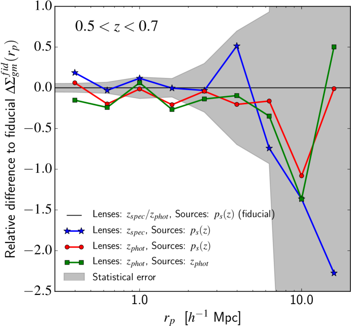
We find that the estimate based on Eq. 11, which only uses maximum likelihood photometric redshifts for both lenses and sources, underestimate the signal on all probed scales by about $15\%$ with respect to the fiducial case. Here, we impose $z_{S}>0.1+z_{L}$, including the additive term of $0.1$ to account for typical photometric redshift errors (e.g. Coupon et al. 2015). Further including the source redshift probability distribution function through the estimator of Eq. 13 allows a slight improvement, reaching an underestimation of about $10\%$ with respect to the fiducial case. The two previous estimates are still affected by the uncertainty on the lens redshifts, which effectively tends to dilute the overall signal. If we now use as lenses only VIPERS spectroscopic galaxies, which represents about $30\%$ of all galaxies with $i_{AB}<22.5$, we find a remarkably good agreement with the fiducial estimate. In principle, this estimate may be considered as the reference unbiased estimate, however on the largest scales probed by the data, i.e. at $r_{p}=10-20\,h^{-1}\leavevmode\nobreak\ {\rm Mpc}$, the signal drops significantly. This can be imputed to the lack of source-lens pairs induced by the reduced number of lenses, directly affecting our ability to probe the largest scales signal. However, we find that this effect can be mitigated by adding photometric lenses from the CFHTLenS catalogue, taking the maximum likelihood photometric redshifts: this corresponds to the fiducial estimate. We note that the expected statistical uncertainty, which is shown in Fig. 2 with the grey shaded area, is not negligible particularly above $r_{p}=10\,h^{-1}\leavevmode\nobreak\ {\rm Mpc}$, and higher than any residual systematic effect. This test makes us confident that our fiducial estimate of $\Delta\Sigma_{gm}(r_{p})$ is robust, given the expected level of statistical error in the data. Similar results are found at $0.7<z<1.2$, leading to the same conclusions.

A non-negligible source of systematics in weak lensing measurements is related to the measurement of background galaxy shapes. This can lead to systematic biases in the lensing measurements. The CFHTLenS collaboration has studied these extensively in Miller et al. (2013) and Heymans et al. (2012), and we follow their method to correct our measurements. We used the additive and multiplicative shear calibration corrections $c$ and $m$, as well as the optimal weights $w^{S}$ provided by lensfit, which are available in the CFHTLenS catalogue. In particular, to correct for the multiplicative bias we applied the correction factor $\left(1+K(r_{p})\right)^{-1}$ to $\Delta\Sigma_{gm}(r_{p})$ as described in Miller et al. (2013) and Velander et al. (2014). We found this correction to boost the galaxy-galaxy lensing signal by about $5\%$ independently of the scale.

For the purpose of constraining the cosmological model, it can be difficult to use $\Delta\Sigma_{gm}$ as its modelling is non-linear. One of the difficulties is to model the non-linear scales and the intrinsic mixing of small-scale non-linear and large-scale linear information (Baldauf et al. 2010). This is achievable but at the expense of introducing additional nuisance parameters in the model (e.g. Cacciato et al. 2013; More et al. 2015). An alternative approach, which we use in this analysis, consists of using a derived statistic that allows the mitigation of non-linearities: the annular differential surface density $\Upsilon_{gm}$, which is defined as (Baldauf et al. 2010)

$$\Upsilon_{gm}(r_{p},r_{0})=\Delta\Sigma_{gm}(r_{p})-\frac{r^{2}_{0}}{r^{2}_{p}}\Delta\Sigma_{gm}(r_{0}).$$ (14)

This statistic removes the small-scale non-linear contribution of $\Delta\Sigma_{gm}$ below a cut-off radius $r_{0}$. We use this quantity in our analysis and study the impact of the choice of $r_{0}$ in Sect. 5.1.

4 Theoretical modelling

4.1 Galaxy biasing

Galaxies are not faithful tracers of the underlying matter distribution and this has to be taken into account in cosmological analyses, since cosmological models primarily predict matter observables. The modelling of galaxy biasing is simplified when focusing on large scales, where bias can be considered as linear and simply be represented as a constant multiplicative factor in front of the matter power spectrum. This is a common assumption in RSD analyses. In our case, however, the relatively small survey volume means that much of our information lies below fully linear scales; for this reason, and because of the intrinsic non-linearities in the excess surface density $\Delta\Sigma_{gm}$, additional care must be taken to model galaxy biasing. We use a non-linear prescription for galaxy bias based on the cosmological perturbation theory that allows describing it more accurately down to translinear scales. We adopt the non-linear non-local bias model of McDonald & Roy (2009) that relates the galaxy overdensity $\delta_{g}$ and matter overdensity $\delta$ as:

$$\delta_{g}({\bf x}) = b_{1}\delta({\bf x})+\frac{1}{2}b_{2}[\delta^{2}({\bf x})-\sigma^{2}]+\frac{1}{2}b_{s^{2}}[s^{2}({\bf x})-\langle s^{2}\rangle]$$ (15)

$$+O(s^{3}({\bf x})),$$

where $b_{1}$ and $b_{2}$ are the linear and second-order non-linear bias terms, $b_{s^{2}}$ the non-local bias term, $s$ is the tidal tensor term from which non-locality originates. The $\sigma^{2}$ and $\langle s^{2}\rangle$ terms ensure the condition $\langle\delta_{g}\rangle=0$.

4.2 Annular differential excess surface density

The galaxy-galaxy lensing quantity that we observe is the differential excess surface density. It is defined as

$$\Delta\Sigma_{gm}(r_{p})=\overline{\Sigma}_{gm}(r_{p})-\Sigma_{gm}(r_{p}),$$ (16)

where

$$\overline{\Sigma}_{gm}(r_{p})=\frac{2}{r^{2}_{p}}\int^{r_{p}}_{0}\Sigma_{gm}(r)\,r\,dr$$ (17)

and $\Sigma_{gm}(r_{p})$ is the projected surface density defined as

$$\Sigma_{gm}(r_{p})=\Omega_{m}\rho_{c}\int^{\infty}_{-\infty}\left(1+\xi_{gm}(\sqrt{r^{2}_{p}+\chi^{2}}\right)d\chi.$$ (18)

In the above equation, $\Omega_{m}$ is matter energy density and $\chi$ is the radial comoving coordinate. $\Upsilon_{gm}$ can be predicted from $\Delta\Sigma_{gm}$ by using Eq. 14 or directly from the galaxy-matter cross-correlation function as (Baldauf et al. 2010)

$$\Upsilon_{gm}(r_{p})=\int_{0}^{\infty}\xi_{gm}(x)W_{\Upsilon}(x,r_{p},r_{0})dx,$$ (19)

where $W_{\Upsilon}(x,r_{p},r_{0})$ is the window function (Baldauf et al. 2010):

$$W_{\Upsilon}(x,r_{p},r_{0}) = \frac{4x}{r^{2}_{p}}\left(\sqrt{x^{2}-r^{2}_{0}}\Theta(x-r_{0})-\sqrt{x^{2}-r_{p}^{2}}\Theta(x-r_{p})\right)$$ (20)

$$-\frac{2x}{r^{2}_{p}}\left(\frac{r^{2}_{p}\Theta(x-r_{p})}{\sqrt{x^{2}-r^{2}_{p}}}-\frac{r_{0}^{2}\Theta(x-r_{0})}{\sqrt{x^{2}-r^{2}_{0}}}\right),$$

where $\Theta(x)$ is the Heaviside step function.

From these equations one can see explicitly that $\Upsilon_{gm}$ is related to the galaxy-matter cross-correlation function $\xi_{gm}$ or cross-power spectrum $P_{gm}$. If we assume the biasing model of Eq. 15, $P_{gm}$ can be written as (McDonald & Roy 2009)

$$P_{gm}(k) = b_{1}P_{\delta\delta}(k)+b_{2}P_{b2,\delta}(k)+b_{s^{2}}P_{bs2,\delta}(k)$$ (21)

$$+b_{3nl}\sigma^{2}_{3}(k)P_{\rm lin}(k),$$

where $P_{\rm{\delta\delta}}$ is the non-linear matter density-density power spectrum, $b_{3nl}$ is a third-order non-local bias term, $P_{\rm lin}$ is the linear matter power spectrum, and $P_{b2,\delta}$, $P_{bs2,\delta}$ are 1-loop integrals given in Appendix A. In the local Lagrangian picture where one assumes no initial non-local bias, one can predict that the non-local bias terms at later time are related to $b_{1}$ such that (Chan et al. 2012; Saito et al. 2014)

$$b_{s^{2}} = -\frac{4}{7}(b_{1}-1)$$ (22)

$$b_{3nl} = \frac{32}{315}(b_{1}-1).$$ (23)

We adopt these relations and our model has finally two galaxy biasing parameters: $b_{1}$ and $b_{2}$, $b_{1}$ being the standard linear bias parameter.

4.3 Redshift-space distortions

The most general formalism describing the redshift-space anisotropies in the power spectrum derives from writing the matter density conservation in real and redshift space (Kaiser 1987). In particular, in the plane-parallel approximation that is assumed in this analysis, the anisotropic power spectrum of matter has the general compact form (Scoccimarro et al. 1999)

$$P^{s}(k,\nu) = \int\frac{\mathrm{d}^{3}\@vec{r}}{(2\pi)^{3}}e^{-i\@vec{k}\cdot\@vec{r}}\left<e^{-ikf\nu\Delta u_{\parallel}}\times\right.$$ (24)

$$\left.[\delta(\@vec{x})+f\partial_{{}_{\parallel}}u_{{}_{\parallel}}(\@vec{x})][\delta(\@vec{x}^{\prime})+f\partial_{{}_{\parallel}}u_{{}_{\parallel}}(\@vec{x}^{\prime})]\right>$$

where $\nu=k_{\parallel}/k$, $u_{\parallel}(\@vec{r})=-v_{\parallel}(\@vec{r})/(faH(a))$, $v_{\parallel}(\@vec{r})$ is the line-of-sight component of the peculiar velocity, $\delta$ is the matter density field, $\Delta u_{\parallel}=u_{\parallel}(\@vec{x})-u_{\parallel}(\@vec{x}^{\prime})$ and $\@vec{r}=\@vec{x}-\@vec{x}^{\prime}$. It is worth noting that in Fourier space, for an irrotational velocity field, $\smash{\partial_{{}_{\parallel}}u_{{}_{\parallel}}}$ is related to the divergence of the velocity field $\theta$ via $\smash{\partial_{{}_{\parallel}}u_{{}_{\parallel}}(\@vec{k})=\nu^{2}\theta(\@vec{k})}$. Although exact, Eq. 24 is impractical and we use the approximation proposed by Taruya et al. (2010). In the case of perfect matter tracers, the latter model takes the form

$$P^{s}(k,\nu) = D(k\nu\sigma_{v})\left[P_{\rm{\delta\delta}}(k)+2\nu^{2}fP_{\rm{\delta\theta}}(k)+\nu^{4}f^{2}P_{\rm{\theta\theta}}(k)\right.$$ (25)

$$\left.+C_{A}(k,\nu,f)+C_{B}(k,\nu,f)\right],$$

where $D(k\nu\sigma_{v})$ is a damping function, $P_{\rm{\delta\delta}}$, $P_{\rm{\delta\theta}}$, $P_{\rm{\theta\theta}}$ are respectively the non-linear matter density-density, density-velocity divergence, and velocity divergence-velocity divergence power spectra, and $\sigma_{v}$ is an effective pairwise velocity dispersion that we can fit for and then treat as a nuisance parameter. The expressions for $C_{A}(k,\nu,f)$ and $C_{B}(k,\nu,f)$ are given in Taruya et al. (2010); de la Torre & Guzzo (2012). This phenomenological model can be seen in configuration space as a convolution of a pairwise velocity distribution, the damping function $D(k\mu\sigma_{v})$ that we assume to be Lorentzian in Fourier space, i.e.

$$D(k\nu\sigma_{v})=(1+k^{2}\nu^{2}\sigma^{2}_{v})^{-1},$$ (26)

and a term involving the density and velocity divergence correlation functions and their spherical Bessel transforms.

This model can be generalized to the case of biased tracers by including a biasing model. By introducing that of Eq. 15, one obtains for the redshift-space galaxy power spectrum (Beutler et al. 2014; Gil-Marín et al. 2014)

$$P_{g}^{s}(k,\nu) = D(k\nu\sigma_{v})\left[P_{\rm{gg}}(k)+2\nu^{2}fP_{\rm{g\theta}}(k)+\nu^{4}f^{2}P_{\rm{\theta\theta}}(k)\right.$$ (27)

$$\left.+C_{A}(k,\nu,f,b_{1})+C_{B}(k,\nu,f,b_{1})\right]$$

where

$$P_{gg}(k) = b_{1}^{2}P_{\delta\delta}(k)+2b_{2}b_{1}P_{b2,\delta}(k)+2b_{s^{2}}b_{1}P_{bs2,\delta}(k)$$ (28)

$$+b_{2}^{2}P_{b22}(k)+2b_{2}b_{s^{2}}P_{b2s2}(k)+b_{s^{2}}^{2}P_{bs22}(k)$$

$$+2b_{1}b_{3\rm nl}\sigma_{3}^{2}(k)P_{\rm lin}(k)+N,$$

$$P_{g\theta}(k) = b_{1}P_{\delta\theta}(k)+b_{2}P_{b2,\theta}(k)+b_{s^{2}}P_{bs2,\theta}(k)$$ (29)

$$+b_{3\rm nl}\sigma_{3}^{2}(k)P_{\rm lin}(k).$$

In the above equations $P_{\rm{\delta\theta}}$ is the non-linear matter density-velocity divergence power spectrum, $P_{\rm lin}$ is the matter linear power spectrum, and $P_{b2,\delta}$, $P_{bs2,\delta}$, $P_{b2,\theta}$, $P_{bs2,\theta}$, $P_{b22}$, $P_{b2s2}$, $P_{bs22}$, $\sigma_{3}^{2}$ are 1-loop integrals given in Appendix A.

The final model for $\xi^{s}_{\ell}(s)$ is obtained from its Fourier counterpart $P^{s}_{\ell}(k)$ defined as

$$P^{s}_{\ell}(k)=\frac{2\ell+1}{2}\int_{-1}^{1}P_{g}^{s}(k,\nu)L_{\ell}(\nu)\,\mathrm{d}\nu,$$ (30)

where

$$\xi^{s}_{\ell}(s)=i^{\ell}\int\frac{k^{2}}{2\pi^{2}}P^{s}_{\ell}(k)j_{\ell}(ks)\,\mathrm{d}k.$$ (31)

In the above equation, $j_{\ell}$ denotes the spherical Bessel functions.

The ingredients of the model are the non-linear power spectra of density and velocity divergence at the effective redshift of the sample. These power spectra can be predicted from perturbation theory or simulations for different cosmological models. The non-linear matter power spectrum can also be obtained to a great accuracy from semi-analytical prescriptions such as HALOFIT (Smith et al. 2003), for various cosmologies. In particular, HALOFIT allows the prediction of $P_{\rm{\delta\delta}}$ from the linear matter power spectrum and the knowledge of the scale of non-linearity at the redshift of interest, $k_{\rm nl}(z)$. We note that at fixed linear matter power spectrum shape, variations of $\sigma_{8}(z)$ can be straightforwardly mapped into variations of $k_{\rm nl}(z)$ (see Smith et al. 2003). In this analysis, the linear matter power spectrum is predicted using the CLASS Boltzmann code (Lesgourgues 2011), and we use the latest calibration of HALOFIT by Takahashi et al. (2012) to obtain $P_{\rm{\delta\delta}}$. To predict $P_{\rm{\theta\theta}}$ and $P_{\rm{\delta\theta}}$, we use the nearly universal fitting functions of Bel et al. (2017) that depend on the linear power spectrum and $\sigma_{8}(z)$ as

$$P_{\rm{\theta\theta}}(z) = P_{\rm lin}(z)e^{-km_{1}\sigma^{m_{2}}_{8}(z)}$$ (32)

$$P_{\rm{\delta\theta}}(z) = \left(P_{\rm{\delta\delta}}(z)P_{\rm lin}(z)e^{-kn_{1}\sigma^{n_{2}}_{8}(z)}\right)^{1/2},$$ (33)

where $P_{\rm lin}$ is the linear power spectrum and $(m_{1},m_{2},n_{1},n_{2})$ are free parameters calibrated on simulations. We adopt here the values $(m_{1},m_{2},n_{1},n_{2})=(1.906,2.163,2.972,2.034)$. These predictions for $P_{\rm{\theta\theta}}$ and $P_{\rm{\delta\theta}}$ are accurate at the few percent level up to $k\simeq 0.7$ (Bel et al. 2017). Therefore, the overall degree of non-linearity in $P_{\rm{\delta\delta}}$, $P_{\rm{\delta\theta}}$ and $P_{\rm{\theta\theta}}$ is solely controlled by $\sigma_{8}(z)$, which is left free when fitting the model to observations.

In the model, the linear bias and growth rate parameters, $b_{1}$ and $f$, are degenerate with the normalization of the matter power spectrum parameter $\sigma_{8}$. Generally with RSD, only the combination of $b_{1}\sigma_{8}$ and $f\sigma_{8}$ can be constrained if no assumption is made on the actual value of $\sigma_{8}$. However in the Taruya et al. (2010) model, $b_{1}^{2}f\sigma_{8}^{4}$, $b_{1}f^{2}\sigma_{8}^{4}$, and $f^{3}\sigma_{8}^{4}$ terms appear in the correction term $C_{A}$ (see Taruya et al. 2010; de la Torre & Guzzo 2012). Accordingly, in the general case, $(f,b_{1},b_{2},\sigma_{8},\sigma_{v})$ are treated as separate parameters in the fit and we provide marginalized constraints on the derived $f\sigma_{8}$.

4.4 Redshift errors

Redshift errors can potentially affect the anisotropic RSD signal. In the anisotropic correlation function they have a similar effect as galaxy random motions in virialized objects: they introduce a smearing of the correlation function along the line of sight at small transverse separations. If the probability distribution function of redshift errors is known, their effect can be forward modelled by adding another multiplicative damping function in the redshift-space galaxy power spectrum of Eq. 19. In that case, the damping function should be the Fourier transform of the error probability distribution function. We follow this approach and the final model is obtained by multiplying Eq. 19 by a Gaussian with standard deviation set to the estimated pairwise redshift dispersion of VIPERS galaxies such that the final RSD model $\smash{\widehat{P_{g}^{s}}}$ reads

$$\widehat{P_{g}^{s}}(k,\nu)=G(k\nu\sigma_{z})P_{g}^{s}(k,\nu),$$ (34)

where $P_{g}^{s}(k,\nu)$ is taken from Eq. 27, $G$ is the Fourier transform of the Gaussian kernel

$$G(k\nu\sigma_{z})=\exp\left(-\frac{k^{2}\nu^{2}\sigma^{2}_{z}}{2}\right),$$ (35)

and $\sigma_{z}$ is the pairwise standard deviation associated with the redshift error probability distribution function.

Figure 3: Probability distribution function of redshift errors at $0.5<z<0.7$ and $0.7<z<1.2$ in the VIPERS data. This is obtained from the redshift differences of reobserved galaxies, for which there are two independent redshift measurements. The dotted and dashed curves are best-fitting Gaussians for the redshift intervals $0.5<z<0.7$ and $0.7<z<1.2$ respectively.

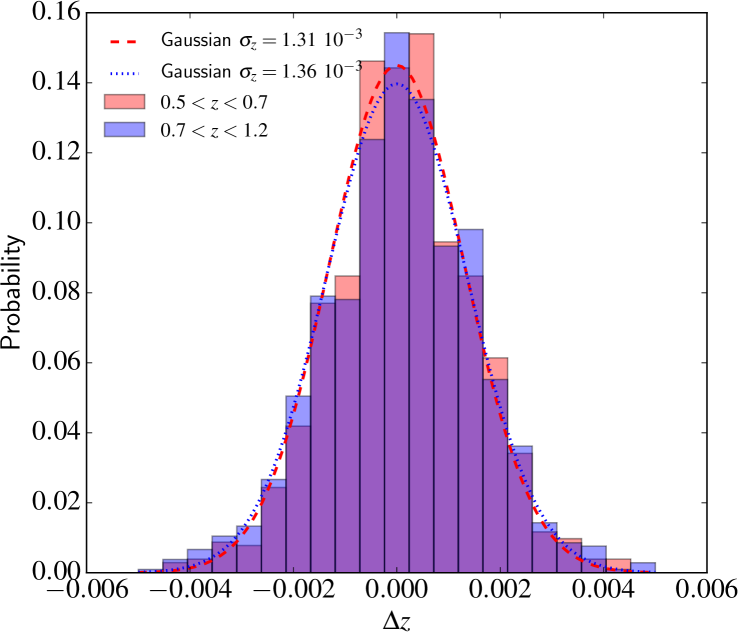
The Gaussian form is motivated by the data themselves as shown in Fig. 3. In this figure are shown the distributions of redshift differences at $0.5<z<0.7$ and $0.7<z<1.2$ in VIPERS reobservations ($1061$ at $0.5<z<0.7$ and $1086$ at $0.7<z<1.2$), for which we have two independent redshift measurements for the same galaxies (see Scodeggio et al. 2017). These distributions can be rather well modelled by Gaussians, and by doing so, we obtain values of $\sigma_{z}=1.31\times 10^{-3}$ and $\sigma_{z}=1.36\times 10^{-3}$ for the pairwise redshift standard deviations at $0.5<z<0.7$ and $0.7<z<1.2$ respectively. These are further converted in comoving length assuming the fiducial cosmology to enter the model in Eq. 34.

4.5 Alcock-Paczynski effect

Additional distortions can arise in galaxy clustering because of the need to assume a fiducial cosmology to convert redshift and angular positions into comoving distances, and the fact that this fiducial cosmology is not necessarily the true one. This is the Alcock & Paczynski (1979) effect (AP). More specifically, since the line-of-sight separations require the knowledge of the Hubble parameter, $H(z)$, and transverse separations that of the angular diameter distance, $D_{A}(z)$, any difference in $H(z)$ and $D_{A}(z)$ between the fiducial and true cosmologies, translates into an anisotropic clustering, independently of RSD. Although AP and RSD anisotropies are degenerate to some extent in the observables (Ballinger et al. 1996; Matsubara & Suto 1996), they have a fundamentally different origin: AP is sensitive to the geometry whereas RSD are sensitive to the growth of cosmological perturbations.

We follow Xu et al. (2013) and model AP distortions using the $\alpha$ and $\epsilon$ parameters, which characterize respectively the isotropic and anisotropic distortion components associated with AP. These are given by

$$\alpha = \left(\frac{D^{2}_{A}}{D^{\prime 2}_{A}}\frac{H^{\prime}}{H}\right)^{1/3}$$ (36)

$$\epsilon = \left(\frac{D^{\prime}_{A}}{D_{A}}\frac{H^{\prime}}{H}\right)^{1/3}-1,$$ (37)

where quantities calculated in the fiducial cosmology are denoted with primes. Those parameters modify the scales at which the correlation function is measured such that

$$r_{\parallel}^{\prime} = \alpha(1+\epsilon)^{2}r_{\parallel}$$ (38)

$$r_{\perp}^{\prime} = \alpha(1+\epsilon)^{-1}r_{\perp}.$$ (39)

Therefore, for the model correlation function monopole and quadrupole in a tested cosmology, the corresponding quantities in the fiducial cosmology are obtained as (Xu et al. 2013)

$$\xi^{\prime}_{0}(s^{\prime}) = \xi_{0}(\alpha s)+\frac{2}{5}\epsilon\left[3\xi_{2}(\alpha s)+\frac{d\xi_{2}(\alpha s)}{d\ln(s)}\right]$$ (40)

$$\xi^{\prime}_{2}(s^{\prime}) = 2\epsilon\frac{d\xi_{0}(\alpha s)}{d\ln(s)}+\bigg{(}1+\frac{6}{7}\epsilon\bigg{)}\xi_{2}(\alpha s)+\frac{4}{7}\epsilon\frac{d\xi_{2}(\alpha s)}{d\ln(s)}$$ (41)

$$+\frac{4}{7}\epsilon\bigg{[}5\xi_{4}(\alpha s)+\frac{d\xi_{4}(\alpha s)}{d\ln(s)}\bigg{]}.$$

In the case of the galaxy-galaxy lensing statistic that we are considering, since it is a function of the transverse separation $r_{p}$, the corresponding $\Upsilon_{gm}$ in the fiducial cosmology is simply given by

$$\Upsilon^{\prime}_{gm}(r^{\prime}_{p})=\Upsilon_{gm}\left(\alpha(1+\epsilon)^{-1}r_{p}\right).$$ (42)

4.6 Cosmological insights from galaxy clustering and galaxy-galaxy lensing

Gravitational physics on cosmological scales can be tested from measurements of the growth rate of structure, which is well measured from RSD in the galaxy clustering pattern. We have seen that in practice, the correlation function multipole moments depend not only on the growth rate of structure $f$, but also on the shape and amplitude $\sigma_{8}$ of the matter power spectrum, the galaxy bias parameters $b_{1}$ and $b_{2}$, and the pairwise velocity dispersion $\sigma_{v}$. To derive the growth rate of structure, one then needs to marginalise over those nuisances. This is of course a source of uncertainty in the determination of the growth rate of structure. Moreover, since there is a degeneracy between the amplitude of the matter power spectrum $\sigma_{8}$, the growth rate of structure $f$, and the linear bias parameter $b_{1}$, RSD alone are sensitive to the $f\sigma_{8}$ and $b_{1}\sigma_{8}$ parameter combinations.

On the other hand, galaxy-galaxy lensing probes the real-space galaxy-matter correlations that are described by the shape and amplitude $\sigma_{8}$ of the matter power spectrum, the galaxy bias parameters $b_{1}$ and $b_{2}$, and the matter density parameter $\Omega_{m}$. Projected galaxy-galaxy correlations are also sensitive to $\sigma_{8}$, $b_{1}$, and $b_{2}$. But by looking in detail at those dependencies, we can see that in the linear regime $\Upsilon_{gm}\propto\Omega_{m}b_{1}\sigma^{2}_{8}$, while $\Upsilon_{gg}\propto b^{2}_{1}\sigma^{2}_{8}$, such that by combining the two we can break the degeneracy between $b_{1}$ and $\sigma_{8}$. We note that $\xi(s,\mu)$, from which $\xi_{0}$ and $\xi_{2}$ are derived, has the same parameter dependences as $\Upsilon_{gg}$, except for the additional $f$ dependence. Therefore, additional galaxy-galaxy lensing information brings an independent handle on the bias parameters $b_{1}$ and $b_{2}$, and the power spectrum amplitude $\sigma_{8}$, reducing the uncertainties on the growth rate of structure induced by the lack of knowledge on the bias of galaxies, as well as a supplementary sensitivity to $\Omega_{m}$.

5 Tests on simulated data

5.1 Simulated data

To test the robustness of redshift-space galaxy clustering, galaxy-galaxy lensing, and associated error estimates, we make use of a large number of mock galaxy samples, which are designed to be a realistic match to the VIPERS final dataset. We used the mock lensing lightcones presented in Giocoli et al. (2016). These have been built upon the Big MultiDark dark matter N-body simulation (Klypin et al. 2016), which assumes a flat $\Lambda{\rm CDM}$ cosmology with $(\Omega_{m},\leavevmode\nobreak\ \Omega_{\Lambda},\leavevmode\nobreak\ \Omega_{b},\leavevmode\nobreak\ h,\leavevmode\nobreak\ n,\leavevmode\nobreak\ \sigma_{8})=(0.307,0.693,0.0482,0.678,0.960,0.823)$ and covers a volume of $15.625\,h^{-3}\leavevmode\nobreak\ {\rm Gpc^{3}}$. These lightcones contain the shear information associated with simulated background galaxies distributed uniformly on the sky but following the redshift distribution of CFHTLenS galaxies. More specifically, the lightcones have been built to match the effective number density and redshift distribution of the CFHTLenS lensing catalogue. We added Gaussian random errors with standard deviation $\smash{\sigma_{e}=(\sigma_{e_{1}}^{2}+\sigma_{e_{2}}^{2})^{1/2}=0.38}$ to the ellipticities to mimic those in the CFHTLenS data. The size of the simulation allowed us to create $54$ independent lightcones for W1 and W4, spanning the redshift range $0<z<2.3$ (for details, see Giocoli et al. 2016).

We populate these lightcones with foreground galaxies using the halo occupation distribution (HOD) technique and apply the detailed VIPERS selection function and observational strategy. The haloes were identified in the simulation using a friends-of-friends algorithm with a relative linking length of $b=0.17$ times the inter-particle separation. The mass limit to which the halo catalogues are complete is $10^{11.95}\,h^{-1}\leavevmode\nobreak\ {\rm M_{\odot}}$. Because this limiting mass is too large to host the faintest galaxies observed with VIPERS, we use the method of de la Torre & Peacock (2013) to reconstruct haloes below the resolution limit. This method is based on stochastically resampling the halo number density field using constraints from the conditional halo mass function. For this, one needs to assume the shapes of the halo bias factor and halo mass function at masses below the resolution limit and use the analytical formulae obtained by Tinker et al. (2008, 2010). With this method we are able to populate the simulation with low-mass haloes with a sufficient accuracy to have unbiased galaxy two-point statistics in the simulated catalogues (for details, see de la Torre et al. 2013). The minimum reconstructed halo mass we consider for the purpose of creating VIPERS mocks is $10^{10}\,h^{-1}\leavevmode\nobreak\ {\rm M_{\odot}}$.

In this process, we populate each halo with galaxies according to its mass, the mean number of galaxies in a halo of a given mass being given by the HOD. It is common usage to differentiate between central and satellite galaxies in haloes. While the former are put at rest at halo centres, the latter are randomly distributed within each halo according to a NFW radial profile (Navarro et al. 1996, 1997). The halo occupation function and its dependence on redshift and luminosity/stellar mass must be precisely chosen in order to obtain mock catalogues with realistic galaxy clustering properties. We calibrated the halo occupation function directly on the VIPERS data, as presented in de la Torre et al. (2013). We add velocities to the galaxies and measure their redshift-space positions. While the central galaxies are assigned the velocity of their host halo, satellite galaxies have an additional random component for which each Cartesian velocity component is drawn from a Gaussian distribution with a standard deviation that depends on the mass of the host halo. Details about the galaxy mock catalogue construction technique are given in Appendix A of de la Torre et al. (2013).

The final step in obtaining fully realistic VIPERS mocks is to add the detailed survey selection function. We start by applying the magnitude cut $i_{\rm AB}<22.5$ and the effect of the colour selection on the radial distribution of the mocks. This is achieved by depleting the mocks at $z<0.6$ so as to reproduce the VIPERS colour sampling rate (see Guzzo et al. 2014, for detail). The mock catalogues that we obtain are then similar to the parent photometric sample in the data. We next apply the slit-positioning algorithm with the same setting as for the data. This allows us to reproduce the VIPERS footprint on the sky, the small-scale angular incompleteness and the variation of ${\rm TSR}$ across the fields. Finally, a random redshift error is added to the redshifts as in the data. We are thus able to produce realistic mock galaxy catalogues that contain the detailed survey completeness function and observational biases of VIPERS, which we refer to as the ‘observed’ mock catalogues in the following.

We note that another set of VIPERS mock catalogues spanning the redshift range of $0.4<z<1.2$ have been constructed. This set, which comprises $306$ and $549$ lightcones of W1 and W4 fields respectively, has not been explicitly used in this analysis, but in accompanying VIPERS PDR-2 analyses (e.g. Hawken et al. 2017; Pezzotta et al. 2017; Wilson et al. 2017; Rota et al. 2017).

5.2 Systematics on the correlation function monopole and quadrupole

Figure 4: Relative systematic errors on the correlation function monopole (top panel) and quadrupole (bottom panel) at $0.5<z<0.7$ and effects of target sampling rate (${\rm TSR}$) and angular pair weighting ($w^{A}$) corrections. The grey shaded areas represent the relative statistical error expected in the survey, while light grey band mark $\pm 1\%$ relative uncertainties for reference.

Figure 5: Same as in Fig. 4 but for the redshift interval $0.7<z<1.2$.

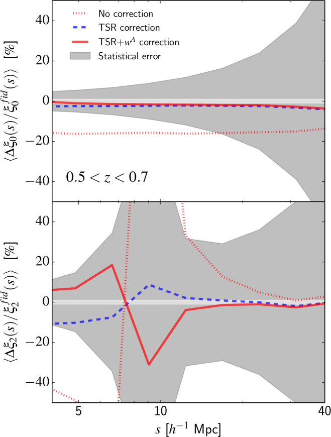
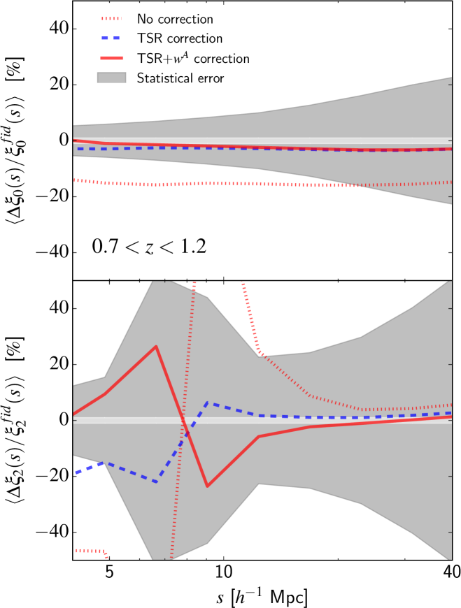
The mock samples are crucial for testing the redshift-space clustering estimation in VIPERS, which is not trivial given the complex selection function of the survey. We first study the impact of the survey selection function on the measurement of the monopole and quadrupole correlation functions. We measured these quantities in the observed mocks, applying the different weights defined in Sect. 3.1, and compare them to the reference measurements obtained from the parent mocks, including VIPERS typical spectroscopic redshift errors. The relative differences in $\xi_{0}$ and $\xi_{2}$ as a function of separation and averaged over the mocks are shown in Figs. 4 and 5, respectively for the two samples at $0.5<z<0.7$ and $0.7<z<1.2$. First of all, it is clear from these figures that without any correction the spectroscopic strategy introduces biases in the estimation of the galaxy clustering. But when applying the survey completeness weights $w^{C}$, one can recover within a few percent the correct amplitude of the correlation functions on scales above $5\,h^{-1}\leavevmode\nobreak\ {\rm Mpc}$. By further applying the angular weights $w^{A}$, we obtain an almost unbiased estimate of the monopole and quadrupole down to a few $\,h^{-1}\leavevmode\nobreak\ {\rm Mpc}$. The statistical relative error induced by sample variance and estimated from the dispersion among the mock samples, is shown with the shaded area in these figures. It is important to note that it is much larger than any residual systematics over the range of scales considered. Finally, it is worth mentioning that in the quadrupole, the apparent higher level of systematics at around $s=10\,h^{-1}\leavevmode\nobreak\ {\rm Mpc}$ is an artefact due to the zero crossing of the functions at slightly different separations.

5.3 Systematics on the growth rate of structure

Figure 6: Relative systematic error on $f\sigma_{8}$ at $0.5<z<0.7$ as a function of $s_{\rm min}$, for different values of $r_{0}$ ($r_{0}=1\,h^{-1}\leavevmode\nobreak\ {\rm Mpc}$ and $r_{0}=1.5\,h^{-1}\leavevmode\nobreak\ {\rm Mpc}$) and when including or not redshift error. The error bars represent the relative statistical error associated to analysing the mean mock predictions. The shaded area shows the $1\sigma$ confidence region associated with the relative statistical error expected in VIPERS. The squares and triangles are artificially shifted along $s_{\rm min}$ axis to improve the clarity of the figure.

We further study our ability to determine $f\sigma_{8}$ when combining RSD and galaxy-galaxy lensing measurements in a maximum likelihood analysis. For this purpose we perform several analyses of the mean RSD and galaxy-galaxy lensing measurements in the observed mocks, for different minimum separations $s_{\rm min}$ in the correlation functions and different cut-off scale $r_{0}$ in the annular differential excess surface density. These analyses are performed on the mean quantities to reduce the impact of statistical errors and concentrate on systematics. The precision matrix is estimated from the mocks as explained in Sect. 6, except that each element is further divided by the number of mocks to characterize the error on the mean. As an illustration, we present in this section only the case of the sample at $0.5<z<0.7$. The sample at $0.7<z<1.2$ provides very similar systematic levels.

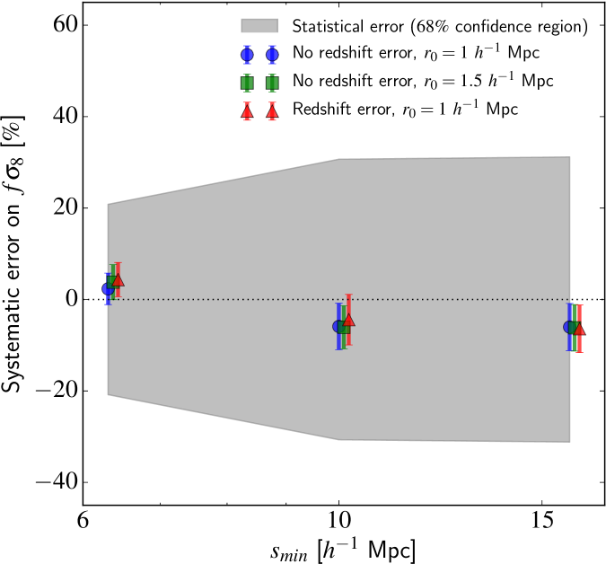
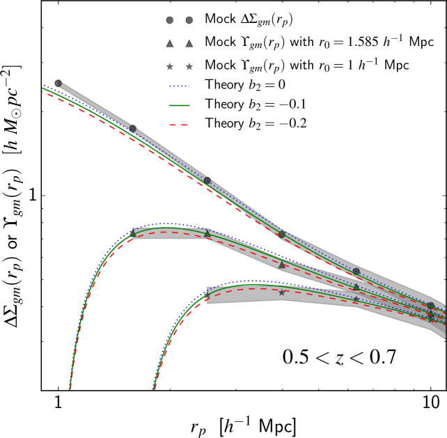
Fig. 6 presents the systematic errors on $f\sigma_{8}$, i.e. the relative difference of recovered values with respect to the fiducial value of the mocks, as a function of $s_{\rm min}$ and for $r_{0}=(1h^{-1}{\rm Mpc},1.5h^{-1}{\rm Mpc})$. We consider rather small minimum scales and cut-off radii to explore the extent to which our modelling is robust in the translinear regime. We can see in this figure that our model allows the recovery of the fiducial value of $f\sigma_{8}$ down to $s_{\rm min}=6.3\,h^{-1}\leavevmode\nobreak\ {\rm Mpc}$, with systematic errors below $5\%$, independently of the choice of $r_{0}$. In principle, values of $r_{0}$ smaller than the typical radius of haloes hosting these galaxies may not be optimal, since the non-linear contribution to correlations may dominate on those scales, which are more difficult to describe (Baldauf et al. 2010). However, this also depends on the galaxy type and the redshift. For VIPERS galaxies and the considered biasing model, we find that $r_{0}=1\,h^{-1}\leavevmode\nobreak\ {\rm Mpc}$ can be well described by our model (see also Blake et al. 2016). This can be seen in Fig. 7 where is shown the comparison between the mean mock $\Delta\Sigma_{gm}$ and $\Upsilon_{gm}$ obtained with $r_{0}=(1h^{-1}{\rm Mpc},1.5h^{-1}{\rm Mpc})$ and the predictions of our model, when $b_{2}$ is allowed to vary and $b_{1}$ is fixed to its fiducial value. We can see that although the model fails to reproduce $\Delta\Sigma_{gm}$ on scales below about $3\,h^{-1}\leavevmode\nobreak\ {\rm Mpc}$, it provides a good description of $\Upsilon_{gm}$ for $b_{2}=-0.1$.

Figure 7: Comparison of differential excess surface density $\Delta_{gm}$ and annular differential excess surface density $\Upsilon_{gm}$ predictions in the mocks (points and shaded regions) and by our theoretical model (curves) at $0.5<z<0.7$. The mock predictions correspond to the mean signal among the mock realizations (points) and its associated $1\sigma$ error (shaded region). The curves show the theoretical predictions for the fiducial parameters of the mocks, varying only the $b_{2}$ parameter as labeled.

We finally test the impact of redshift errors on the recovery of $f\sigma_{8}$ in Fig. 6. This figure shows the relative systematic error on $f\sigma_{8}$ as a function $s_{\rm min}$ in the case where $r_{0}$ is fixed to $1\,h^{-1}\leavevmode\nobreak\ {\rm Mpc}$ and typical VIPERS redshift errors are added randomly to mock galaxy redshifts. By comparing it to the case without redshift errors, we can see that for the RSD model where a Gaussian damping term is added to account for redshift errors, the recovery of $f\sigma_{8}$ is achieved without additional bias, with only a small relative bias of about $3\%$ at $s_{\rm min}=6.3\,h^{-1}\leavevmode\nobreak\ {\rm Mpc}$ and $-5\%$ above. We note that this is the ideal case where the redshift error probability distribution function is perfectly known.

Overall, these tests demonstrate that our model with $s_{\rm min}=6.3\,h^{-1}\leavevmode\nobreak\ {\rm Mpc}$ and $r_{0}=1\,h^{-1}\leavevmode\nobreak\ {\rm Mpc}$ is robust enough to provide a precise measurement of $f\sigma_{8}$ with VIPERS data, with residual systematics of the order of a few per cent only, but only representing about one fifth of expected statistical error on the measurement as shown with the grey shaded region in Fig. 6. Based on these tests, we adopt $(s_{\rm min},r_{0})=(6.3\leavevmode\nobreak\ h^{-1}{\rm Mpc},1\leavevmode\nobreak\ h^{-1}{\rm Mpc})$ values for the following analysis.

6 Likelihood analysis and precision matrix

In order to derive cosmological parameters from the combination of RSD and galaxy-galaxy lensing measurements, we perform a maximum likelihood analysis in which we define the likelihood function $\mathcal{L}$ such that

$$-2\ln{\mathcal{L}}=\sum_{i=1}^{N_{p}}\sum_{j=1}^{N_{p}}\Delta_{i}\hat{C}^{-1}_{ij}\Delta_{j},$$ (43)

where $N_{p}$ is the number of data points in the fit, $\bf\Delta$ is the data-model difference vector, and $\smash{{\bf\hat{C}^{-1}}}$ is the inverse data covariance matrix. $\bf\Delta$ is defined such that each element is $\Delta_{i}=d_{i}-m_{i}$, where $\bf d$ and $\bf m$ are respectively the data and model prediction vectors. In our case, $\bf d$ is the concatenation of $\xi_{0}$, $\xi_{2}$, and $\Upsilon_{gm}$, for the set of considered separations. The parameter space of the model is explored using a Monte Carlo Markov Chain (MCMC) method implementing the Metropolis-Hastings algorithm (Metropolis et al. 1953).

A robust estimation of the inverse data covariance matrix, or precision matrix, is crucial in order to achieve realistic posterior likelihood functions of the parameters. The different bins in $\xi_{0}$, $\xi_{2}$, and $\Upsilon_{gm}$ are correlated to some degree and this must be allowed for in the likelihood analysis. We measure these three quantities in the $54$ mocks and estimate the covariance matrix $\bf C$. The generic elements of the matrix can be evaluated as

$$C_{ij}=\frac{1}{N_{m}-1}\sum_{k=1}^{N_{m}}\left(d^{k}_{i}-\bar{d_{i}}\right)\left(d^{k}_{j}-\bar{d_{j}}\right)\,,$$ (44)

where $N_{m}$ is the number of mock realizations and the indices $i,j$ run over the data vector $\bf d$ elements. An unbiased estimate of the inverse covariance matrix, ${\bf\hat{C}^{-1}}$, is obtained as (Hartlap et al. 2007)

$${\bf\hat{C}^{-1}}=\frac{N_{m}-N_{p}-2}{N_{m}-1}{\bf C}^{-1},$$ (45)

for $N_{m}>N_{p}-2$. The resulting inverse covariance matrix obtained from mock realizations can be noisy, depending on how large $N_{m}$ is with respect to $N_{p}$. In our case, $N_{m}=54$ and $N_{p}=16$, which suggests the presence of a non-negligible noise in the inverse covariance matrix. In order to reduce the level of noise, we adopt the tapering technique of Kaufman et al. (2008). This technique has been introduced in the context of cosmological analysis by Paz & Sánchez (2015). This technique relies on the assumption that large-scale covariances vanish, and consists of tapering the covariance matrix around the diagonal using a specific positive and compact taper function. Contrary to other estimators such as shrinkage (e.g. Pope & Szapudi 2008), the two-tapers estimator has the advantage of being unbiased. The inverse tapered covariance matrix is obtained as

$${\bf\hat{C_{T}}^{-1}}=\left(\frac{N_{m}-N_{p}-2}{N_{m}-1}\right)({\bf C}\circ{\bf T})^{-1}\circ{\bf T},$$ (46)

where ‘$\circ$’ denotes the element-wise matrix product and ${\bf T}$ is the tapering matrix. We follow Paz & Sánchez (2015) and use the tapering matrix defined as

$$T_{ij}=K(|{\bf x}_{i}-{\bf x}_{j}|),$$ (47)

where $x_{i}$ is the $i^{th}$ measurement position in the data vector, and $K$ is the taper function that we take to be a Wendland function:

$$K(x)=\left\{\begin{array}[]{lcl}\left(1-\frac{x}{T_{p}}\right)^{4}\left(4\frac{x}{T_{p}}+1\right)\hskip 14.22636pt{\rm if}\leavevmode\nobreak\ x<T_{p}\\ \\ 0\hskip 85.35826pt\rm{otherwise}.\end{array}\right.$$ (51)

This taper function has one free parameter, the tapering scale $T_{p}$, which essentially represents the typical scale difference above which covariances are nullified.

Figure 8: Top panel: recovered errors on $f\sigma_{8}$ normalized to that obtained without tapering (equivalent to applying tapering with $T_{p}=\infty$), as a function of the tapering scale $T_{p}$ used in the estimation of the precision matrix. This is obtained from the mocks at $0.5<z<0.7$. Bottom panel: recovered maximum likelihood values for $f\sigma_{8}$ and associated $1\sigma$ error as a function of the tapering scale $T_{p}$.

Figure 9: Correlation matrix (left panel) and normalized precision matrix (right panel) for galaxy clustering and galaxy-galaxy lensing data in the redshift interval $0.5<z<0.7$. These are defined as $C_{ij}/\sqrt{C_{ii}C_{jj}}$ and $C^{-1}_{ij}/\sqrt{C^{-1}_{ii}C^{-1}_{jj}}$ respectively, where $C_{ij}$ and $C^{-1}_{ij}$ refer to covariance and precision matrix elements respectively. In both panels, the upper triangular matrix represents the case without tapering, while the lower panel the case with tapering. The precision matrix is normalized such that diagonal elements are unity.

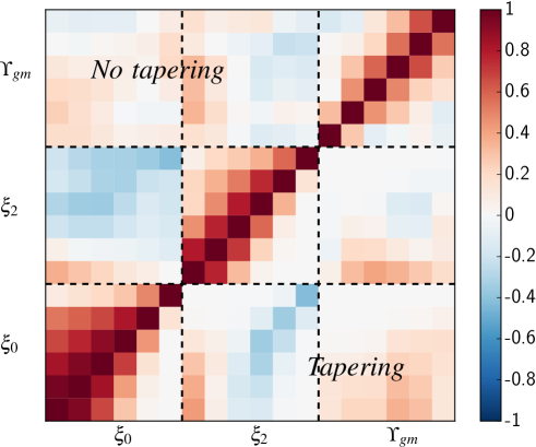
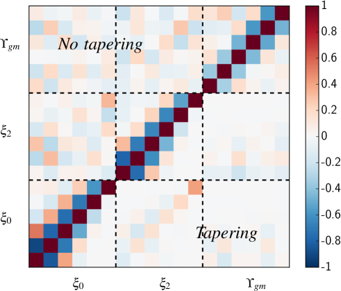
In our case, the covariance matrix is associated with three different quantities as well as two different separation types, $s$ and $r_{p}$. One would then potentially need to use a combination of several taper functions, since one does not expect the large-scale covariance to vanish at the same scales for all quantities. Although it may be sub-optimal to use a single taper function, we still expect to increase the signal-to-noise, and since the estimator is unbiased, one cannot introduce additional bias or error. We therefore decided to use a single taper function for simplicity.

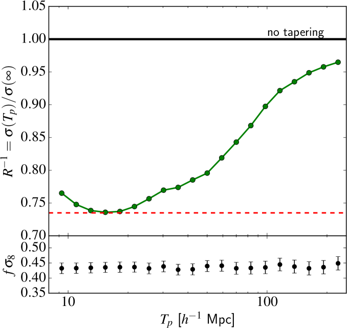
In the general case, it is not straightforward to define a priori the optimal tapering scale. Paz & Sánchez (2015) introduced a simple empirical method, which consists of performing several maximum likelihood analyses of the data varying only the tapering scale, and taking as the optimal $T_{p}$ the one that minimizes the error on the parameter of interest. We perform the same exercise on the mean mock predictions. The marginalized $1\sigma$ error on $f\sigma_{8}$ as a function of $T_{p}$ is presented in the top panel of Fig. 8. We can see that the $T_{p}$ value that minimizes the error is around $15\,h^{-1}\leavevmode\nobreak\ {\rm Mpc}$, and we adopt this value in our analysis. We also verified that the maximum likelihood values for $f\sigma_{8}$ remain unchanged for any value of $T_{p}$ as shown in the bottom panel of Fig. 8.

To illustrate the method, we present in Fig. 9 the correlation matrix and normalized precision matrix, for the combined RSD and galaxy-galaxy lensing data in the redshift interval $0.5<z<0.7$, when applying or not the tapering technique (lower and upper triangles respectively). Those matrices are defined as $C_{ij}/\sqrt{C_{ii}C_{jj}}$ and $C^{-1}_{ij}/\sqrt{C^{-1}_{ii}C^{-1}_{jj}}$ respectively, where $C_{ij}$ and $C^{-1}_{ij}$ refer to covariance and precision matrix elements respectively. We can see the reduction of noise, which is particularly clear in the normalized precision matrix for most off-diagonal terms.

The tapering technique allows a significant reduction of the noise level in the precision matrix, but cannot completely remove it. The remaining noise can propagate through the likelihood analysis into derived parameter uncertainties. In order to obtain realistic confidence limits on parameters one needs to account for the additional uncertainties coming from the precision matrix estimation (Taylor & Joachimi 2014). Percival et al. (2014) showed that this additional error can be described as a rescaling of the target parameter covariance, in the case when the precision matrix is estimated with the standard estimator of Eq. 45. But the appropriate degree of rescaling is unclear when the tapering estimator is used. The improvement on the error that we find with the tapering estimator (i.e. $26.5\%$) is similar to or larger than what we would expect with the standard estimator using $300$ mocks or more as predicted by (Dodelson & Schneider 2013; Percival et al. 2014). This gives us confidence that only a small correction, if any, would be necessary.

7 Cosmological results

The comprehensive tests of the methodology described in previous sections make us confident that we can perform a robust combined analysis of RSD and galaxy-galaxy lensing with VIPERS and CFHTLenS dataset, and infer cosmology from it. We present in this section the data measurements, growth rate of structure constraints, and derived gravitational slip parameters at $0.5<z<0.7$ and $0.7<z<1.2$.

7.1 Galaxy clustering and galaxy-galaxy lensing measurements

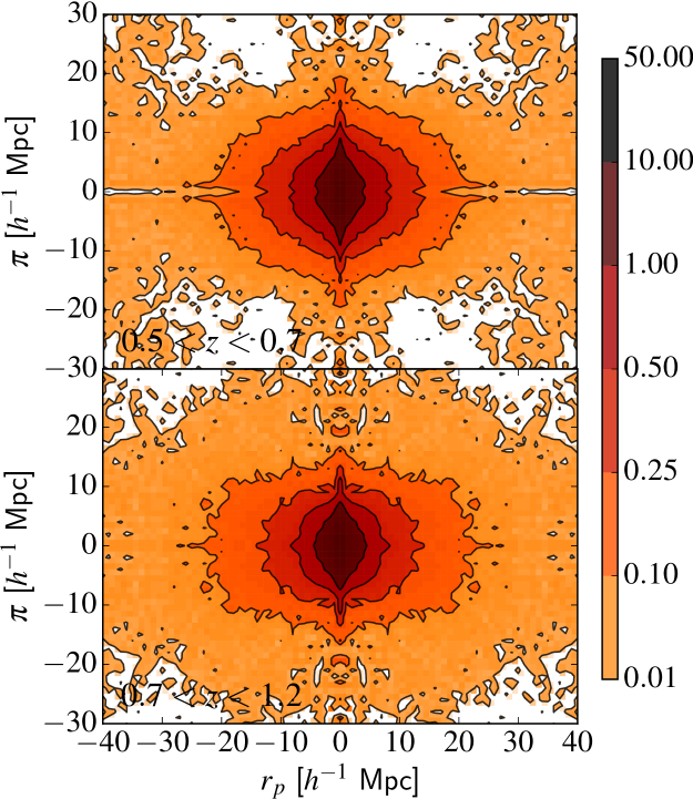
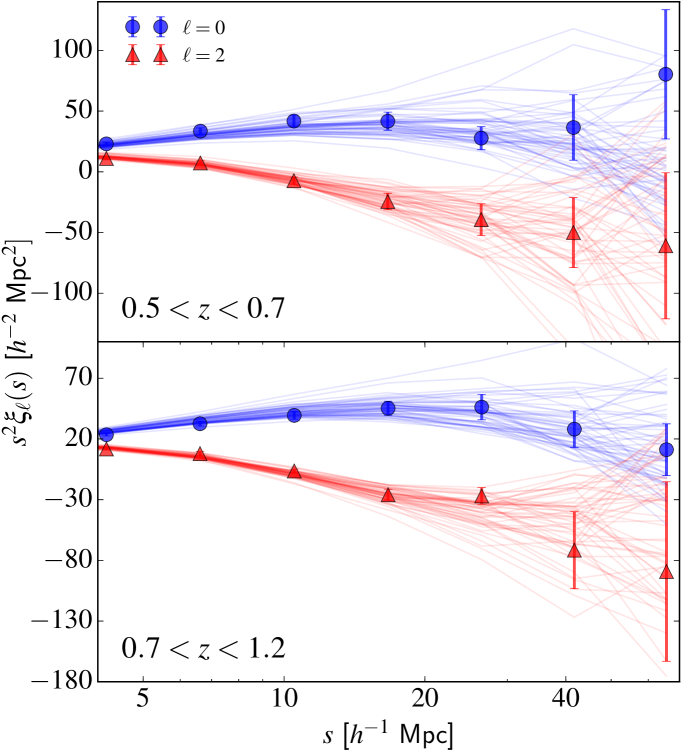
The correlation function measurements are performed on the full VIPERS galaxy sample in the redshift intervals $0.5<z<0.7$ and $0.7<z<1.2$. We select all VIPERS galaxies above the limiting magnitude of the survey, and measure the monopole and quadrupole correlation functions in both W1 and W4 fields. The combined W1+W4 measurements are obtained by summing up the pairs in the two fields, contributing to the anisotropic two-point correlation functions $\xi(s,\mu)$, before deriving $\xi_{0}$ and $\xi_{2}$ from Eq. 2. The full anisotropic two-point correlation functions are presented in Fig. 10, and the monopole and quadrupole moments in Fig. 11. In the latter figure, the individual mock measurements are superimposed, giving a visual appreciation of the error associated with these measurements in VIPERS. We can see that the combined W1+W4 monopole and quadrupole correlation function measurements enable us to probe accurately the redshift-space galaxy clustering signal on scales below about $s=50\,h^{-1}\leavevmode\nobreak\ {\rm Mpc}$.

Figure 10: Anisotropic correlation functions of VIPERS galaxies at $0.5<z<0.7$ (top panel) and $0.7<z<1.2$ (bottom panel) as a function parallel and transverse to the line-of-sight separations.

Figure 11: Monopole (circles) and quadrupole (triangles) correlation functions of VIPERS galaxies at $0.5<z<0.7$ (top panel) and $0.7<z<1.2$ (bottom panel). Solid curves correspond to individual mock measurements.

The differential excess surface density measurements are obtained by combining W1 and W4 individual field measurements in a similar fashion. The lens galaxies are taken from the VIPERS catalogue or the CFHTLenS catalogue if no spectroscopic redshift is available. They are selected to have $i_{\rm AB}<22.5$ and a redshift in the intervals $0.5<z<0.7$ and $0.7<z<1.2$. The source galaxies are taken from the CFHTLenS catalogue and are selected to have $i_{\rm AB}<24.1$. The differential excess surface density and annular differential excess surface density measurements for $r_{0}=1\,h^{-1}\leavevmode\nobreak\ {\rm Mpc}$ are presented in Fig. 12. As in Fig. 11, the individual mock measurements are superimposed. We can see that with the combined W1+W4 annular differential excess surface density measurements we can reach scales up to about $r_{p}=20\,h^{-1}\leavevmode\nobreak\ {\rm Mpc}$.

Figure 12: Differential excess surface density (circles) and annular differential excess surface density (triangles) at $0.5<z<0.7$ (top panel) and $0.7<z<1.2$ (bottom panel). Solid curves correspond to individual mock measurements.

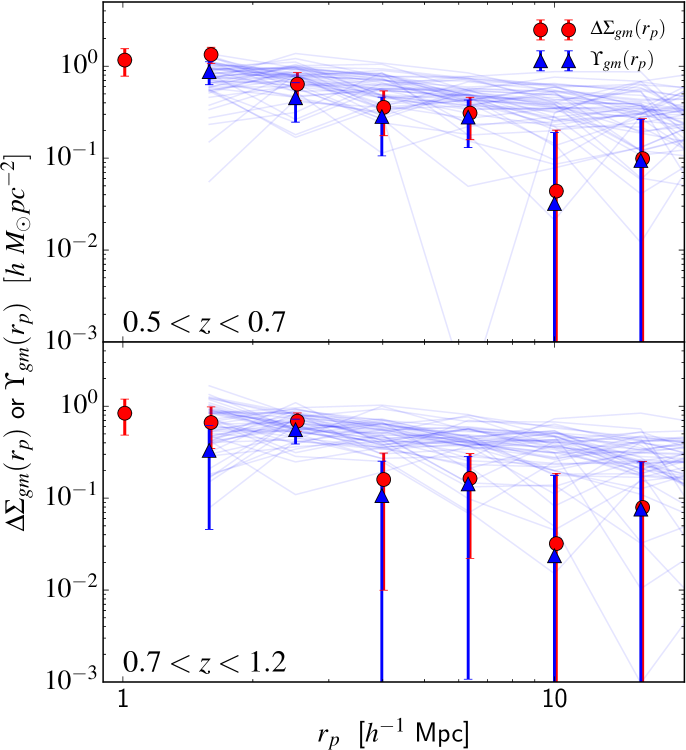
Our $\Upsilon_{gm}$ measurements are more uncertain than the $\xi_{0}$ and $\xi_{2}$ ones. This is essentially related to the way the former are estimated. Weak lensing is fundamentally limited by the unknown intrinsic ellipticity of the sources, which dominates the error budget. This can be mitigated by means of a larger number of sources. Given the surface density of sources in our sample and its rather modest angular coverage of $23.5\leavevmode\nobreak\ \rm{deg}^{2}$, we obtain relative errors on $\Upsilon_{gm}$ of about $25\%$, estimated from the mock samples. In contrast, the typical relative error that we obtain on $\xi_{0}$ is of $5\%$. Therefore, in our combined analysis of the RSD and galaxy-galaxy lensing we expect $\Upsilon_{gm}$ to have a much lower weight in the likelihood. We finally remark that the observed $\Upsilon_{gm}$ tend to exhibit lower amplitudes than expected in the mock samples, in particular in the highest redshift interval. We discuss the cosmological implications of this in Sect. 7.3.

7.2 Growth of structure constraints

We perform a combined maximum likelihood analysis of the monopole, quadrupole, and annular differential excess surface density to derive constraints on the growth rate of structure at $0.5<z<0.7$ and $0.7<z<1.2$. The effective redshifts associated with these intervals are $z=0.6$ and $z=0.86$. They correspond to the average redshift of pairs contributing the most to monopole and quadrupole correlation functions in these redshift intervals (Samushia et al. 2014). The theoretical model that we use is described in Sect. 4; it depends on 11 parameters, ${\bf p}=(f,b_{1},b_{2},\sigma_{v},\sigma_{8},\epsilon,\alpha,\Omega_{m},\Omega_{m}h^{2},\Omega_{b}h^{2},n_{s})$. The last three describe the shape of the matter power spectrum and these are determined most accurately by CMB data. Since our galaxy clustering and weak lensing measurements cannot provide such tight constraints on these parameters, we fix them to the best-fitting Planck 2015 TT+lowP+lensing parameters (Planck Collaboration et al. 2016). Consistently, $\Omega_{m}$ is kept fixed to the Planck value in $\Upsilon_{gm}$. Possible departures from those parameter values are only allowed through variations of the AP distortion parameters $\epsilon$ and $\alpha$. In the following, we first consider measurements of $f\sigma_{8}$, as a derived parameter, and later study the possibility of deriving independent measurements of $f$ and $\sigma_{8}$. All those measurements are obtained by marginalizing over the nuisance parameters: ${\bf p_{n}}=(b_{1},b_{2},\sigma_{v},\epsilon,\alpha)$. The adopted uniform priors on the likelihood parameters are summarized in Table LABEL:tab and the full posterior likelihood contours for the cases presented in the next section are given in Appendix B.

Table 1: Adopted priors on the likelihood parameters.

Parameters	Uniform prior
$b_{1}$	$[0.5,2]$
$b_{2}$	$[-1,1]$
$\sigma_{v}$	$[0,8]$
$f$	$[0.2,1.4]$
$\sigma_{8}$	$[0,1.2]$
$\epsilon$	$[-0.1,0.1]$
$\alpha$	$[0.9,1.1]$

7.2.1 $f\sigma_{8}$ measurements

In our standard configuration, the linear matter power spectrum shape is fixed to the best-fitting $\Lambda\rm{CDM}$ model from Planck 2015 TT+lowP+lensing data (Planck Collaboration et al. 2016). AP distortion parameters are set to $(\epsilon,\alpha)=(0,1)$ and are not allowed to vary. In this configuration we obtain $f\sigma_{8}$ values of

$$f\sigma_{8}(z=0.6) = 0.48\pm 0.12$$ (52)

$$f\sigma_{8}(z=0.86) = 0.48\pm 0.10,$$ (53)

after marginalizing over other parameters. Associated reduced chi-squared values are $\chi^{2}_{\nu}=1.52$ and $\chi^{2}_{\nu}=1.62$ respectively. These measurements use both RSD and galaxy-galaxy lensing information. It is instructive to see the impact of adding the galaxy-galaxy lensing on the measurement of $f\sigma_{8}$. Thus if we use the standard RSD approach without including galaxy-galaxy lensing information, we obtain

$$f\sigma_{8}(z=0.6) = 0.48\pm 0.11$$ (54)

$$f\sigma_{8}(z=0.86) = 0.46\pm 0.09,$$ (55)

with a reduced chi-squared value of $\chi^{2}_{\nu}=1.12$ for both redshifts. In that case, we fixed $b_{2}=b_{s^{2}}=b_{3nl}=0$ in the RSD model, as bias non-linearities are negligible for VIPERS galaxies bias given the minimum scale used in the fit (Pezzotta et al. 2017). Moreover, the shape of non-linear power spectra in the model is fixed by setting $\sigma_{8}$ to its fiducial value at the effective redshift of the sample, as is commonly done (e.g. de la Torre et al. 2013). The recovered values and associated errors are very similar to the previous case. We do not find an improvement on $f\sigma_{8}$ accuracy when galaxy-galaxy lensing is included, in fact errors are marginally larger. This can be explained by the lower number of degrees of freedom in the RSD-only case and the significant uncertainty associated with our galaxy-galaxy lensing measurements compared to the galaxy clustering ones in the VIPERS fields. In fact the real gain is on contraining $f$ and $\sigma_{8}$ separately as discussed in Sect. 7.2.4.

7.2.2 Inclusion of Alcock-Paczynski distortions

As a robustness test, we relax the assumption on the shape of the linear matter power spectrum. We allow the AP distortion parameters $(\epsilon,\alpha)$ to vary, considering flat priors on $\epsilon,\alpha$ parameters, extending by $\pm 0.1$ around $(\epsilon,\alpha)=(0,1)$. After marginalizing over those parameters as well, we obtain the following $f\sigma_{8}$ measurements:

$$f\sigma_{8}(z=0.6) = 0.51\pm 0.13,$$ (56)

$$f\sigma_{8}(z=0.86) = 0.52\pm 0.11,$$ (57)

with reduced chi-squared values of $\chi^{2}_{\nu}=1.58$ and $\chi^{2}_{\nu}=1.3$ respectively. As expected from the additional degrees of freedom introduced in the likelihood, the marginalized $68\%$ errors on $f\sigma_{8}$ are increased, although the constraints remain completely compatible with previous measurements when $\epsilon$ and $\alpha$ were fixed. This test thus removes any potential concern that our measurements of $f\sigma_{8}$ might lack robustness though being dependent on the assumption of a $\Lambda\rm{CDM}$ expansion history.

7.2.3 Comparison with other measurements

In Fig. 13 we compare our $f\sigma_{8}$ measurements with previous measurements from the literature, as well as predictions of the standard relativistic model for gravity. Our measurements are consistent with previous measurements at lower or similar redshifts from VVDS (Guzzo et al. 2008), SDSS LRG (Cabré & Gaztañaga 2009; Samushia et al. 2012), WiggleZ (Blake et al. 2012), 6dFGS (Beutler et al. 2012), VIPERS PDR-1 (de la Torre et al. 2013), MGS (Howlett et al. 2015), FastSound (Okumura et al. 2016), BOSS-LOWZ (Gil-Marín et al. 2016), and BOSS-CMASS (Gil-Marín et al. 2016; Chuang et al. 2016). In particular, our measurement at $z=0.6$ is compatible within $1\sigma$ with the WiggleZ $z=0.6$ (Blake et al. 2012) and BOSS-CMASS $z=0.57$ (Gil-Marín et al. 2016; Chuang et al. 2016) measurements. Our results are also very close to the standard cosmological model predictions: they are consistent within $1\sigma$ with General Relativity predictions in a $\Lambda\rm{CDM}$ model with cosmological parameters set to Planck CMB results (Planck Collaboration et al. 2016).

Figure 13: $f\sigma_{8}$ as a function of redshift, showing VIPERS results contrasted with a compilation of recent measurements. The previous results from VVDS (Guzzo et al. 2008), SDSS LRG (Cabré & Gaztañaga 2009; Samushia et al. 2012), WiggleZ (Blake et al. 2012), 6dFGS (Beutler et al. 2012), VIPERS PDR-1 (de la Torre et al. 2013), MGS (Howlett et al. 2015), FastSound (Okumura et al. 2016), BOSS-LOWZ (Gil-Marín et al. 2016), BOSS-CMASS (Gil-Marín et al. 2016; Chuang et al. 2016), and VIPERS PDR-2 voids (Hawken et al. 2017) are shown with the different symbols (see labels). The solid curve and associated shaded area correspond to the expectations and $68\%$ uncertainty for General Relativity in a $\Lambda\rm{CDM}$ background model set to TT+lowP+lensing Planck 2015 predictions (Planck Collaboration et al. 2016).

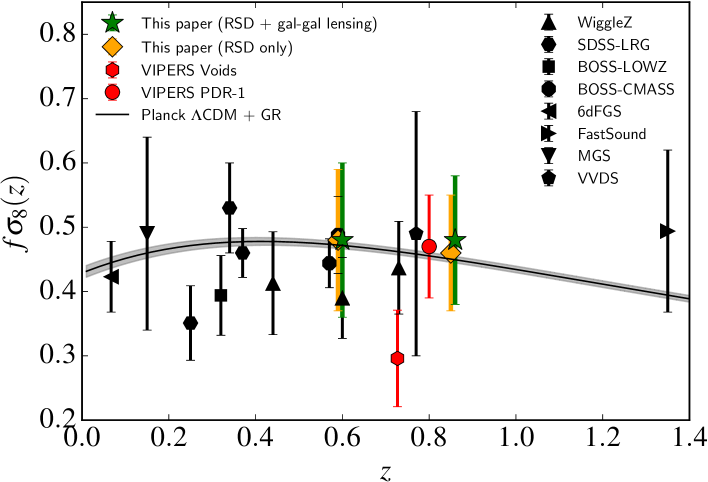
These results are part of a combined effort of the VIPERS collaboration to estimate the growth rate of structure from the same data but using different complementary techniques. Specifically, in Pezzotta et al. (2017) we provide a thorough investigation of the performances of different RSD models in configuration space, using a general consistent modelling of non-linear RSD; in Wilson et al. (2017) we use the clipping technique in Fourier space to minimise the impact of non-linearities; finally in Hawken et al. (2017) we use cosmic voids as RSD tracers. In particular in Hawken et al. (2017), we make use of the void catalogue built from the VIPERS PDR-2 data and resulting from the earlier work by Micheletti et al. (2014), to estimate the void-galaxy cross-correlation function in redshift space. By modelling its anisotropy we obtain an estimate of $f\sigma_{8}$ at $z=0.73$ and derive a value of $f\sigma_{8}(z=0.73)=0.296^{+0.075}_{-0.078}$, which is lower than those obtained here. However, this technique is still in its infancy, with potential systematic errors not yet fully understood. This and the other VIPERS measurements are all fully compatible within statistical errors. More discussion is presented in the specific papers.

7.2.4 $f,b_{1},\sigma_{8}$ degeneracy breaking

Figure 14: Two-dimensional marginalized posterior likelihood contours for $f$ and $\sigma_{8}$ at $0.5<z<0.7$, showing the impact of the additional galaxy-galaxy lensing constraint on the $f-\sigma_{8}$ degeneracy. The black curve shows the region of constant $f\sigma_{8}$ associated with Planck Collaboration et al. (2016) ${\rm\Lambda CDM+GR}$ best-fit, while the combined $(f,\sigma_{8})$ constraint is marked with the star.

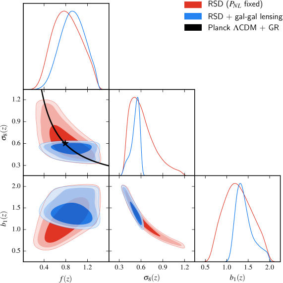
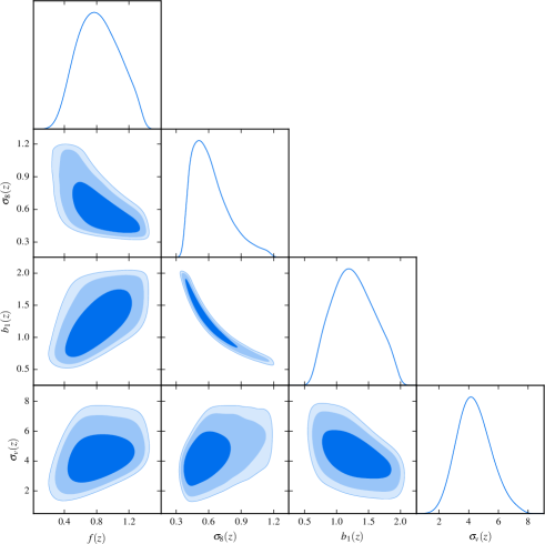
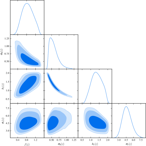
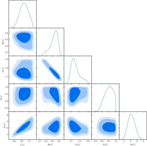
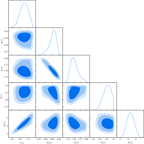
As discussed in Sect. 4, the use of RSD in the galaxy clustering pattern allows a measurement of the parameter combinations $f\sigma_{8}$, $b_{1}\sigma_{8}$, or $\beta=f/b_{1}$. But with the additional constraint of galaxy-galaxy lensing, which exhibits different parameter dependencies, we expect to be able to break the $f-b_{1}-\sigma_{8}$ degeneracy inherent to galaxy-galaxy correlations. We investigate this by studying the posterior likelihood contours at $68\%,95\%,99\%$ for the various pairs of $f$, $b$, $\sigma_{8}$ parameters in our data. This is done for the likelihood analyses presented in the previous sections, i.e. when including or not galaxy-galaxy lensing. The posterior likelihood contours are presented in Figs. 14 and 15 for the two considered redshift intervals.

Figure 15: Same as Fig. 14 but for the redshift interval $0.7<z<1.2$.

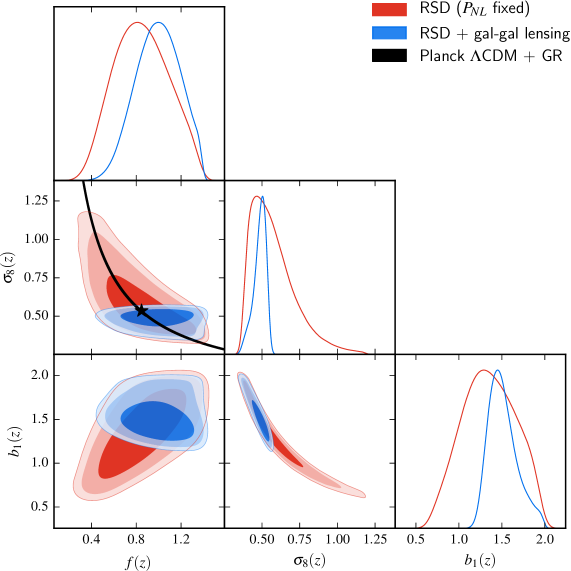
These figures show strong degeneracies in the $f-b_{1}$, $f-\sigma_{8}$, and $b_{1}-\sigma_{8}$ planes when considering only RSD. In particular, we can see in the $f-\sigma_{8}$ plane the distribution of the likelihood contours along the regions with constant $f\sigma_{8}$, marked with solid and dashed curves in the figures. Now with the inclusion of galaxy-galaxy lensing, we can see a shrinking of the contours, in particular along the $\sigma_{8}$ direction, and to a lesser extent along the $b_{1}$ one. Galaxy-galaxy lensing thus effectively provides a strong handle on the $\sigma_{8}$ parameter. This allows the $f-\sigma_{8}$ degeneracy to be broken and therefore leads to the possibility of a direct measurement of the growth rate of structure, $f$. The $f-b_{1}$ degeneracy is also partially broken, even if the effect is milder.

We find that the $f-\sigma_{8}$ degeneracy breaking is more efficient in the high-redshift interval, with measurements of $(f,\sigma_{8})=(0.93\pm 0.22,0.52\pm 0.06)$ and $(f,\sigma_{8})=(0.99\pm 0.19,0.48\pm 0.04)$ at $z=0.6$ and $z=0.86$ respectively. These direct measurements of the growth rate of structure and $\sigma_{8}$ are in agreement within $1\sigma$ with Planck ${\rm\Lambda CDM+GR}$ predictions, which are $(f,\sigma_{8})=(0.79,0.60)$ and $(f,\sigma_{8})=(0.85,0.53)$ respectively at $z=0.6$ and $z=0.86$. Planck ${\rm\Lambda CDM+GR}$ predictions are represented with the stars in Figs. 14 and 15. In Fig. 16, we compare our $(f,\sigma_{8})$ constraints with those from Gil-Marín et al. (2017), obtained by combining redshift-space galaxy power spectrum and bispectrum information in the BOSS survey at $z=0.57$. In Gil-Marín et al. (2017), they use the galaxy bispectrum instead of galaxy-galaxy lensing to bring additional constraints on galaxy bias. Although those measurements are quite uncertain, this parameter space and how it can be used as a cosmological model diagnostic, will be very interesting to explore for next-generation cosmological surveys, such as Euclid, which will allow a dramatical improvement on such measurement accuracy.

Figure 16: Joint $(f,\sigma_{8}$) constraints at different redshifts. The combined RSD and galaxy-galaxy lensing posterior likelihood contours at $1\sigma$ and $2\sigma$ and those from Gil-Marín et al. (2017), obtained by combining redshift-space power spectrum and bispectrum information in the BOSS survey, are presented. The solid curve and associated grey shaded area correspond to the expectations and $68\%$ uncertainty for General Relativity in a $\Lambda\rm{CDM}$ background model set to TT+lowP+lensing Planck 2015 predictions (Planck Collaboration et al. 2016), as a function of redshift from $z=2$ to $z=0$.

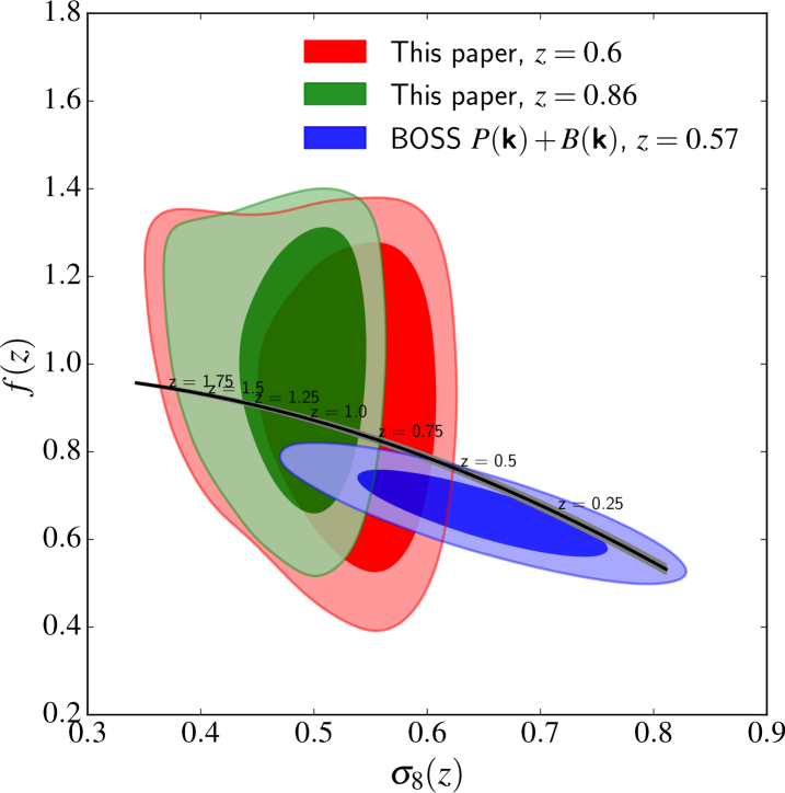
Independent measurements of $\sigma_{8}$ at different redshifts also carry information about the growth rate of structure. Since $\sigma_{8}$ grows with time proportionally to the growth factor, the growth rate can be written as $\mathrm{d}\ln\sigma_{8}/\mathrm{d}\ln a$. In the case of two $\sigma_{8}$ measurements at $a_{1}$ and $a_{2}$, as in our analysis, this equation can be approximated through finite difference by

$$f\simeq\frac{\ln\left(\sigma_{8}(a_{1})/\sigma_{8}(a_{2})\right)}{\ln\left(a_{1}/a_{2}\right)}.$$ (58)

By applying this to our $\sigma_{8}$ measurements we obtain an additional, independent measurement of $f=0.57\pm 0.96$ at the mean redshift of $z=0.73$. It is clear that this type of measurement is not compelling in our dataset, but can potentially be useful as an additional constraint to be combined with direct measurements in next-generation cosmological surveys.

Finally, we notice in Figs. 14 and 15 that the addition of galaxy-galaxy lensing constraints significantly modifies the posterior probability distribution function of the linear bias parameter, $b_{1}$, becoming more compact and skewed towards larger values. This means that adding galaxy-galaxy lensing information reduces the uncertainties on $b_{1}$, and pushes its maximum likelihood value towards values that are in excellent agreement with previous linear bias estimates that are not solely based on two-point statistics (Di Porto et al. 2016; Cappi et al. 2015; Granett et al. 2015).

7.3 Gravitational slip

In addition to the growth rate of structure, we can measure the gravitational slip parameter $E_{G}$. This is done by taking the ratio of the measured $\Upsilon_{gm}$ and $\Upsilon_{gg}$, and multiplying it by $\beta^{-1}$. The RSD distortion parameter $\beta$ is estimated from the combined maximum likelihood analysis of the monopole and quadrupole correlation functions (the same as for the RSD-only case presented in Sect. 7.2.1). After marginalizing over nuisance parameters we obtain

$$\beta(z=0.6) = 0.66\pm 0.17$$ (59)

$$\beta(z=0.86) = 0.63\pm 0.14.$$ (60)

The $68\%$ error on the $E_{G}$ measurements is obtained by adding in quadrature the fractional error on $\Upsilon_{gm}/\Upsilon_{gg}$ estimated from mock samples and the fractional error on $\beta^{-1}$.

The $E_{G}(r_{p})$ measurements are presented in Fig. 17 for the two redshift intervals under consideration, and compared with the linear predictions for ${\rm\Lambda CDM+GR}$ (horizontal line and associated $68\%$ contour). We find that our measurements at $z=0.6$ are compatible within $1\sigma$ with the standard model, although the central values tend to be slightly lower. We also report in this figure the averaged gravitational slip parameter over the range $3\,h^{-1}\leavevmode\nobreak\ {\rm Mpc}$¡$r_{p}$¡$50\,h^{-1}\leavevmode\nobreak\ {\rm Mpc}$, $\smash{\overline{E}_{G}}$, obtained by Blake et al. (2016) in the similar redshift range $0.43<z<0.7$. It is represented with a stripe in the figure, with horizontal extent corresponding to the range of $r_{p}$ used to measure $\smash{\overline{E}_{G}}$ and vertical extent showing the $\pm 1\sigma$ error on the measurement. By averaging our $E_{G}$ over $3\,h^{-1}\leavevmode\nobreak\ {\rm Mpc}$¡$r_{p}$¡$20\,h^{-1}\leavevmode\nobreak\ {\rm Mpc}$ we obtain $\smash{\overline{E}_{G}}(z=0.6)=0.16\pm 0.09$ and $\smash{\overline{E}_{G}}(z=0.86)=0.09\pm 0.07$. Our results are in good agreement with this measurement and also with that by Pullen et al. (2016) at much higher scales, which also exhibits a slightly lower value compared with ${\rm\Lambda CDM+GR}$ prediction. The $E_{G}$ measurements are lower than ${\rm\Lambda CDM+GR}$ at $r_{p}>3\,h^{-1}\leavevmode\nobreak\ {\rm Mpc}$ but remain within $1-2\sigma$, depending on the scale. At $z=0.86$, the agreement with ${\rm\Lambda CDM+GR}$ is poorer than at lower redshift.

Figure 17: Gravitational slip parameter as a function of scale as measured at $0.5<z<0.7$ (top panel) and $0.7<z<1.2$ (bottom panel). In both panels, the solid curves and associated shaded areas correspond to the expectations and $68\%$ uncertainties for General Relativity in a $\Lambda\rm{CDM}$ background model set to TT+lowP+lensing Planck 2015 predictions (Planck Collaboration et al. 2016). In the top panel, the horizontal stripe shows the averaged $\smash{\overline{E}_{G}}$ over the range $3\,h^{-1}\leavevmode\nobreak\ {\rm Mpc}$¡$r_{p}$¡$50\,h^{-1}\leavevmode\nobreak\ {\rm Mpc}$ obtained by Blake et al. (2016) at $0.43<z<0.7$. $E_{G}$ asymptotes to $\Omega_{m}/f$ in the standard model, and the simplest way of erasing the modest discrepancy with the model prediction would be to lower the density parameter.

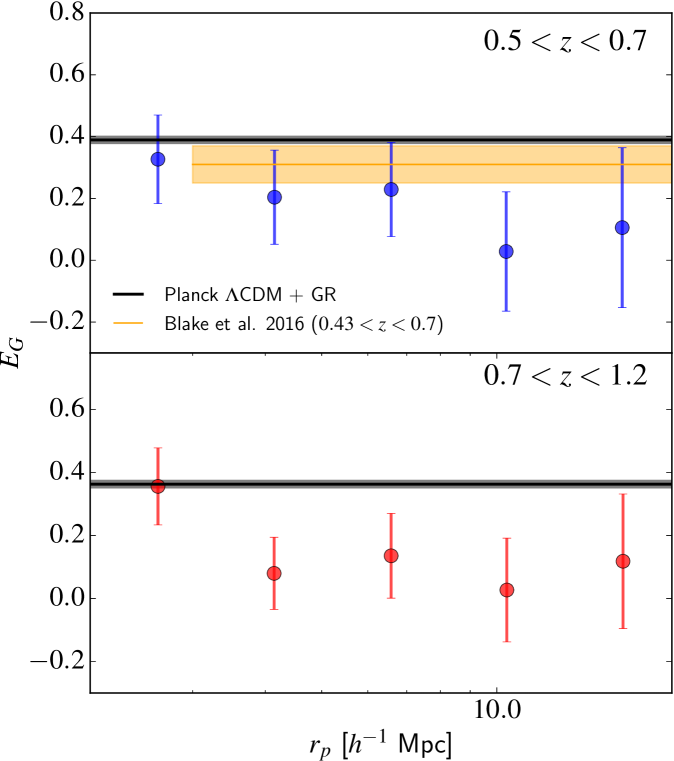
The origin of the tendency of our $E_{G}$ measurements to be smaller than expected at $r_{p}>3\,h^{-1}\leavevmode\nobreak\ {\rm Mpc}$ remains unclear. Particularly given our statistical errors, we have to be cautious in interpreting this trend. In any case, such a result could arise as a result of residual observational systematics or a misinterpretation of the observables, rather than any break-down of standard gravitational physics. From the construction of $E_{G}$, these low values of $E_{G}$ seem to be most probably caused by the rather low measured amplitude of $\Upsilon_{gm}$ at $r_{p}>3\,h^{-1}\leavevmode\nobreak\ {\rm Mpc}$, and seen in Fig. 12. If this discrepancy is upheld by further data, one possible interpretation is that weak lensing prefers a lower value of $\Omega_{m}$ than that determined by CMB data. It is worth noticing that a similar tension has already been identified in the CFHTLenS cosmic shear analysis of Heymans et al. (2013), as well as in the more recent analysis performed in the KiDS lensing survey (Hildebrandt et al. 2017). It is clear that this point needs to be investigated in detail in the future, in particular in the preparation of next-generation very large surveys combining galaxy clustering and weak lensing observables.

8 Conclusion

This paper has presented a combined analysis of redshift-space distortions and galaxy-galaxy lensing in the final VIPERS dataset, making use of complementary data from the CFHTLenS lensing survey over the same area. We have built a consistent theoretical model of the two observables, which includes prescriptions for non-linear, non-local galaxy bias, as well as quasi-linear redshift-space distortions. This model has been shown to enable robust measurements of the growth rate of structure. The model robustness and adopted methodology have been tested by using a series of realistic mock surveys constructed for this purpose.

The main goal of VIPERS has been to provide an accurate measurement of the growth rate of structure using redshift-space distortions in a redshift regime where the growth is not well determined. With the first data release we were able to provide an initial measurement of $f\sigma_{8}$ at $z=0.8$ (de la Torre et al. 2013). The final dataset increases the survey volume by a factor of $1.6$, and by further adding galaxy-galaxy lensing information, we have been able to provide new accurate measurements of $f\sigma_{8}$ at both $z=0.6$ and $z=0.86$. We have found values of $f\sigma_{8}(z=0.6)=0.48\pm 0.12$ and $f\sigma_{8}(z=0.86)=0.48\pm 0.10$, which are consistent with previous measurements at lower or similar redshifts.

The additional galaxy-galaxy lensing constraint and the specific treatment of $\sigma_{8}$ to describe the non-linearity level of the real-space power spectra entering the model alleviate the degeneracy between the galaxy bias parameter, $\sigma_{8}$, and $f$, and has allowed direct measurements of these two parameters. We have obtained values of $\left(f,\sigma_{8}\right)=(0.93\pm 0.22,0.52\pm 0.06)$ and $\left(f,\sigma_{8}\right)=(0.99\pm 0.19,0.48\pm 0.04)$ at $z=0.6$ and $z=0.86$, respectively. These measurements put new constraints on gravity at the epoch when the Universe was almost half its present age. Our measurements are statistically consistent with a Universe where the gravitational interactions between structures on cosmological scales can be described by General Relativity, although they are not yet accurate enough to rule out some commonly considered alternatives to General Relativity.

In addition to measuring the growth rate of structure, we have been able to measure the gravitational slip parameter, $E_{G}$, for the first time at $z>0.6$. This quantity, which can be directly constructed from galaxy clustering and galaxy-galaxy lensing observables, is sensitive to the growth rate of structure and mean matter density in the Universe. We have obtained averaged values of the gravitational slip parameter of $\smash{\overline{E}_{G}}(z=0.6)=0.16\pm 0.09$ and $\smash{\overline{E}_{G}}(z=0.86)=0.09\pm 0.07$. Our $E_{G}$ measurements are consistent within $1-2\sigma$, although they exhibit slightly lower values than expected in the standard model for gravity in a $\Lambda\rm{CDM}$ background.

Overall, this analysis has demonstrated the importance of the combination of galaxy clustering in redshift space and galaxy-galaxy lensing in order to probe the origin of cosmic acceleration. This combination can alleviate the inherent uncertainty related to galaxy bias in RSD analyses and provide new insights into the gravitational physics at work on cosmological scales. This analysis and adopted methodology can be seen as a proof-of-concept in the context of the preparation of next-generation cosmological surveys such as Euclid (Laureijs et al. 2011), which will allow galaxy clustering and galaxy-galaxy lensing to be combined with exquisite precision.

Appendix A Theoretical power spectra for biased tracers

This appendix presents the models describing the real-space galaxy-galaxy, galaxy-velocity divergence, and galaxy-matter power spectra, which enter the modelling of RSD and galaxy-galaxy lensing. We adopt the non-linear non-local bias model of McDonald & Roy (2009) that relates the galaxy overdensity $\delta_{g}$ and matter overdensity $\delta$ as:

$$\delta_{g}({\bf x}) = b_{1}\delta({\bf x})+\frac{1}{2}b_{2}[\delta^{2}({\bf x})-\sigma^{2}]+\frac{1}{2}b_{s^{2}}[s^{2}({\bf x})-\langle s^{2}\rangle]$$ (61)

$$+O(s^{3}({\bf x})).$$

In this equation, $b_{1}$ and $b_{2}$ are the linear and second-order non-linear bias terms, $b_{s^{2}}$ the non-local bias term, $s$ is the tidal tensor term from which non-locality originates. The $\sigma^{2}$ and $\langle s^{2}\rangle$ terms ensure the condition $\langle\delta_{g}\rangle=0$. From the bias model of Eq. 61 one can derive the following power spectra for galaxy-galaxy, galaxy-velocity divergence ($\theta$), and galaxy-matter correlations:

$$P_{gg}(k) = b_{1}^{2}P_{\delta\delta}(k)+2b_{2}b_{1}P_{b2,\delta}(k)+2b_{s^{2}}b_{1}P_{bs2,\delta}(k)$$ (62)

$$+b_{2}^{2}P_{b22}(k)+2b_{2}b_{s^{2}}P_{b2s2}(k)+b_{s^{2}}^{2}P_{bs22}(k)$$

$$+2b_{1}b_{3\rm nl}\sigma_{3}^{2}(k)P_{\rm lin}(k)+N,$$

$$P_{g\theta}(k) = b_{1}P_{\delta\theta}(k)+b_{2}P_{b2,\theta}(k)+b_{s^{2}}P_{bs2,\theta}(k)$$ (63)

$$+b_{3\rm nl}\sigma_{3}^{2}(k)P_{\rm lin}(k),$$

$$P_{gm}(k) = b_{1}P_{\delta\delta}(k)+b_{2}P_{b2,\delta}(k)+b_{s^{2}}P_{bs2,\delta}(k)$$ (64)

$$+b_{3nl}\sigma^{2}_{3}(k)P_{\rm lin}(k),$$

where (e.g. Beutler et al. 2014; Gil-Marín et al. 2014)

$$P_{b2,\delta}(k) = \int\frac{d^{3}q}{(2\pi)^{3}}\,P_{\rm lin}(q)P_{\rm lin}(|{\bf k}-{\bf q}|)F_{2}({\bf q},{\bf k-q}),$$ (65)

$$P_{bs2,\delta}(k) = \int\frac{d^{3}q}{(2\pi)^{3}}\,P_{\rm lin}(q)P_{\rm lin}(|{\bf k}-{\bf q}|)F_{2}({\bf q},{\bf k-q})$$ (66)

$$S_{2}({\bf q},{\bf k-q}),$$

$$P_{b2,\theta}(k) = \int\frac{d^{3}q}{(2\pi)^{3}}\,P_{\rm lin}(q)P_{\rm lin}(|{\bf k}-{\bf q}|)G_{2}({\bf q},{\bf k}-{\bf q}),$$ (67)

$$P_{bs2,\theta}(k) = \int\frac{d^{3}q}{(2\pi)^{3}}\,P_{\rm lin}(q)P_{\rm lin}(|{\bf k}-{\bf q}|)G_{2}({\bf q},{\bf k}-{\bf q})$$ (68)

$$S_{2}({\bf q},{\bf k}-{\bf q}),$$

$$P_{b2s2}(k) = -\frac{1}{2}\int\frac{d^{3}q}{(2\pi)^{3}}\,P_{\rm lin}(q)\left[\frac{2}{3}P_{\rm lin}(q)-P_{\rm lin}(|{\bf k}-{\bf q}|)\right.$$ (69)

$$\left.S_{2}({\bf q},{\bf k}-{\bf q})\right],$$

$$P_{bs22}(k) = -\frac{1}{2}\int\frac{d^{3}q}{(2\pi)^{3}}\,P_{\rm lin}(q)\left[\frac{4}{9}P_{\rm lin}(q)-P_{\rm lin}(|{\bf k}-{\bf q}|)\right.$$ (70)

$$\left.S_{2}({\bf q},{\bf k}-{\bf q})^{2}\right],$$

$$P_{b22}(k) = -\frac{1}{2}\int\frac{d^{3}q}{(2\pi)^{3}}\,P_{\rm lin}(q)\left[P_{\rm lin}(q)-P_{\rm lin}({\bf k}-{\bf q}|)\right],$$ (71)

$$\sigma^{2}_{3}(k) = \int\frac{d^{3}{\bf q}}{(2\pi)^{3}}\,P_{\rm lin}(q)\left[\frac{5}{6}+\frac{15}{8}S_{2}({\bf q},{\bf k}-{\bf q})\right.$$ (72)

$$\left.S_{2}(-{\bf q},{\bf k})-\frac{5}{4}S_{2}({\bf q},{\bf k}-{\bf q})\right].$$

In the above equations, $S_{2}$, $F_{2}$, $G_{2}$ perturbation theory kernels are defined by (e.g. Goroff et al. 1986; Bernardeau et al. 2002)

$$S_{2}({\bf k}_{i},{\bf k}_{j}) = \frac{({\bf k}_{i}\cdot{\bf k}_{j})^{2}}{(k_{i}k_{j})^{2}}-\frac{1}{3},$$ (73)

$$F_{2}({\bf k}_{i},{\bf k}_{j}) = \frac{5}{7}+\frac{1}{2}\frac{{\bf k}_{i}\cdot{\bf k}_{j}}{k_{i}k_{j}}\left(\frac{k_{i}}{k_{j}}+\frac{k_{j}}{k_{i}}\right)+\frac{2}{7}\left[\frac{{\bf k}_{i}\cdot{\bf k}_{j}}{k_{i}k_{j}}\right]^{2},$$ (74)

$$G_{2}({\bf k}_{i},{\bf k}_{j}) = \frac{3}{7}+\frac{1}{2}\frac{{\bf k}_{i}\cdot{\bf k}_{j}}{k_{i}k_{j}}\left(\frac{k_{i}}{k_{j}}+\frac{k_{j}}{k_{i}}\right)+\frac{4}{7}\left[\frac{{\bf k}_{i}\cdot{\bf k}_{j}}{k_{i}k_{j}}\right]^{2}.$$ (75)

Appendix B Posterior likelihood contours

In this appendix are provided the posterior likelihood contours of all pairs of parameters appearing in the likelihood analyses presented in Sect. 7.2.1. Fig. 18 shows the posterior likelihood contours in the case of the RSD-only analysis, while Fig. 19 in the case where RSD and galaxy-galaxy lensing are combined. In both figures, the three types of shaded regions in each subpanel correspond to the posterior likelihood contours at $68\%$, $95\%$, and $99\%$.

Figure 18: Posterior likelihood contours for $f$, $\sigma_{8}$, $b_{1}$, and $\sigma_{v}$ parameters at $z=0.6$ (left panel) and $z=0.86$ (right panel) in the case where RSD are considered alone (see Sect. 7.2.1).

Figure 19: Posterior likelihood contours for $f$, $\sigma_{8}$, $b_{1}$, $b_{2}$, and $\sigma_{v}$ parameters at $z=0.6$ (left panel) and $z=0.86$ (right panel) in the case where RSD and galaxy-galaxy lensing are combined (see Sect. 7.2.1).