Stratified regression-based variance reduction approach for weak approximation schemes

Abstract

In this paper we suggest a modification of the regression-based variance reduction approach recently proposed in Belomestny et al [1]. This modification is based on the stratification technique and allows for a further significant variance reduction. The performance of the proposed approach is illustrated by several numerical examples.

1 Introduction

Let $T>0$ be a fixed time horizon. Consider a $d$-dimensional diffusion process $(X_{t})_{t\in[0,T]}$ defined by the Itô stochastic differential equation

$$dX_{t}=\mu(X_{t})\,dt+\sigma(X_{t})\,dW_{t},\quad X_{0}=x_{0}\in\mathbb{R}^{d}$$

for Lipschitz continuous functions $\mu\colon\mathbb{R}^{d}\to\mathbb{R}^{d}$ and $\sigma\colon\mathbb{R}^{d}\to\mathbb{R}^{d\times m}$, where $(W_{t})_{t\in[0,T]}$ is a standard $m$-dimensional Brownian motion. Suppose we want to compute the expectation

$$u(t,x):=\mathbb{E}[f(X_{T}^{t,x})],$$ (1)

where $X^{t,x}$ denotes the solution to (1) started at time $t$ in point $x$. The standard Monte Carlo (SMC) approach for computing $u(0,x)$ at a fixed point $x\in\mathbb R^{d}$ basically consists of three steps. First, an approximation $\overline{X}_{T}$ for $X^{0,x}_{T}$ is constructed via a time discretisation in equation (1) (we refer to [4] for a nice overview of various discretisation schemes). Next, $N_{0}$ independent copies of the approximation $\overline{X}_{T}$ are generated, and, finally, a Monte Carlo estimate $V_{N_{0}}$ is defined as the average of the values of $f$ at simulated points:

$$V_{N_{0}}:=\frac{1}{N_{0}}\sum_{i=1}^{N_{0}}f\Bigl{(}\overline{X}_{T}^{(i)}\Bigr{)}.$$ (2)

In the computation of $u(0,x)=\mathbb E[f(X^{0,x}_{T})]$ by the SMC approach there are two types of error inherent: the discretisation error $\mathbb E[f(X^{0,x}_{T})]-\mathbb E[f(\overline{X}_{T})]$ and the Monte Carlo (statistical) error, which results from the substitution of $\mathbb E[f(\overline{X}_{T})]$ with the sample average $V_{N_{0}}$. The aim of variance reduction methods is to reduce the statistical error. For example, in the so-called control variate variance reduction approach one looks for a random variable $\xi$ with $\mathbb E\xi=0$, which can be simulated, such that the variance of the difference $f(\overline{X}_{T})-\xi$ is minimised, that is,

$$\operatorname{Var}[f(\overline{X}_{T})-\xi]\to\min\text{ under }\mathbb E\xi=0.$$

Then one uses the sample average

$$V_{N_{0}}^{CV}:=\frac{1}{N_{0}}\sum_{i=1}^{N_{0}}\left[f\Bigl{(}\overline{X}_{T}^{(i)}\Bigr{)}-\xi^{(i)}\right]$$ (3)

instead of (2) to approximate $\mathbb E[f(\overline{X}_{T})]$. The use of control variates for computing expectations of functionals of diffusion processes via Monte Carlo was initiated by Newton [7] and further developed in Milstein and Tretyakov [6]. Heath and Platen [3] use the integral representation to construct unbiased variance-reduced estimators. In Belomestny et al [1] a novel regression-based approach for the construction of control variates, which reduces the variance of the approximated functional $f(\overline{X}_{T})$ was proposed. As shown in [1], the “Monte Carlo approach with the Regression-based Control Variate” (abbreviated below as “RCV approach”) as well as its enhancement, called “recursive RCV (RRCV) approach”, are able to achieve a higher order convergence of the resulting variance to zero, which in turn leads to a significant complexity reduction as compared to the SMC algorithm. The RCV approaches become especially simple in the case of the so-called weak approximation schemes, i.e., the schemes, where simple random variables are used in place of Brownian increments, and which became quite popular in recent years. In this paper we further enhance the performance of the RRCV algorithm by combining it with stratification. The idea of the resulting stratified RCV (SRCV) algorithm is based on partitioning of the state space into a collection of sets $\mathcal{A}_{1},\ldots,\mathcal{A}_{p}$ and then performing conditional regressions separately on each set. It turns out that by choosing $\mathcal{A}_{1},\ldots,\mathcal{A}_{p}$ to be the level sets of the discrete-valued random variables used in the weak approximation scheme, we can achieve a further variance reduction effect as compared to the original approach in [1]. The paper is organised as follows. In Section 2, the SRCV algorithm is introduced and compared with the RCV and RRCV ones. The complexity analysis of the SRCV algorithm is conducted in Section 3. Section 4 is devoted to the simulation study. Necessary proofs are collected in Section 5.

2 SRCV approach and its differences with RCV and RRCV ones

In what follows $J\in\mathbb N$ denotes the time discretisation parameter. We set $\Delta:=T/J$ and consider discretisation schemes denoted by $(X_{\Delta,j\Delta})_{j=0,\ldots,J}$, which are defined on the grid $\{j\Delta:j=0,\ldots,J\}$. In Sections 2.1 and 2.2 we consider weak schemes of order $1$. In this setting we recall the RCV and RRCV algorithms, introduce the SRCV algorithm and explain how it compares to the RCV and RRCV ones. In Section 2.3 we briefly discuss the case of weak schemes of order $2$.

2.1 RCV algorithm for first order schemes

Let us consider a weak scheme of order $1$, where $d$-dimensional approximations $X_{\Delta,j\Delta}$, $j=0,\ldots,J$, satisfy $X_{\Delta,0}=x_{0}$ and

$$X_{\Delta,j\Delta}=\Phi_{\Delta}(X_{\Delta,(j-1)\Delta},\xi_{j}),\quad j=1,\ldots,J,$$ (4)

for some functions $\Phi_{\Delta}\colon\mathbb R^{d+m}\to\mathbb R^{d}$, with $\xi_{j}=(\xi_{j}^{1},\ldots,\xi_{j}^{m})$, $j=1,\ldots,J$, being $m$-dimensional i.i.d. random vectors with i.i.d. coordinates satisfying

$$\mathbb P\left(\xi_{j}^{k}=\pm 1\right)=\frac{1}{2},\quad k=1,\ldots,m.$$

An important particular case is the weak Euler scheme (also called the simplified weak Euler scheme in [4, Section 14.1]), which is given by

$$\Phi_{\Delta}(x,y)=x+\mu(x)\,\Delta+\sigma(x)\,y\,\sqrt{\Delta}.$$ (5)

The RCV approach of [1] essentially relies on the following representation, which has some resemblance to the discrete-time Clark-Ocone formula (see e.g. [8]).

Theorem 1

It holds

$$f(X_{\Delta,T})=\mathbb Ef(X_{\Delta,T})+\sum_{j=1}^{J}\sum_{k\in\{0,1\}^{m}\setminus\{0\}}a_{j,k}(X_{\Delta,(j-1)\Delta})\prod_{i=1}^{m}(\xi_{j}^{i})^{k_{i}},$$ (6)

where $k=(k_{1},\ldots,k_{m})$ and $0=(0,\ldots,0)$ (in the second summation). Moreover, the coefficients $a_{j,k}\colon\mathbb R^{d}\to\mathbb R$ can be computed by the formula

$$a_{j,k}(x)=\mathbb E\left[\left.f(X_{\Delta,T})\prod_{i=1}^{m}(\xi_{j}^{i})^{k_{i}}\,\right|\,X_{\Delta,(j-1)\Delta}=x\right]$$ (7)

for all $j$ and $k$ as in (6).

Theorem 1 is an equivalent reformulation of Theorem 3.1 in [1].

Discussion

Under appropriate conditions on the functions $f$, $\mu$ and $\sigma$ (see e.g. Theorem 2.1 in [5]) the discretisation error $\mathbb E[f(X_{T})]-\mathbb E[f(X_{\Delta,T})]$ for the scheme (5) is of order $\Delta$ (first order scheme). Furthermore, by Theorem 1, with

$$M^{(1)}_{\Delta,T}:=\sum_{j=1}^{J}\sum_{k\in\{0,1\}^{m}\setminus\{0\}}a_{j,k}(X_{\Delta,(j-1)\Delta})\prod_{i=1}^{m}(\xi_{j}^{i})^{k_{i}},$$ (8)

we have $\mathbb E\left[M^{(1)}_{\Delta,T}\right]=0$ and $\operatorname{Var}\left[f(X_{\Delta,T})-M^{(1)}_{\Delta,T}\right]=0$, that is, $M^{(1)}_{\Delta,T}$ is a perfect control variate reducing the statistical error down to zero. However, in practice we cannot simulate $M^{(1)}_{\Delta,T}$ because the coefficients $a_{j,k}$ are generally unknown. In the RCV algorithm, we construct a practically implementable control variate $\tilde{M}^{(1)}_{\Delta,T}$ of the form (8) with regression-based estimates $\tilde{a}_{j,k}\colon\mathbb R^{d}\to\mathbb R$ of the functions $a_{j,k}$. It is worth noting that the sample average of $f(X_{\Delta,T}^{(i)})-\tilde{M}_{\Delta,T}^{(1),(i)}$ (cf. (3)) should be computed on the paths independent of those used to construct $\tilde{a}_{j,k}$. This ensures that $\mathbb E\bigl{[}\tilde{M}^{(1)}_{\Delta,T}\bigr{]}=0$, and, thus, that $\tilde{M}_{\Delta,T}^{(1)}$ is a valid control variate (because of the martingale transform structure in (8)).

2.2 RRCV and SRCV algorithms for first order schemes

The coefficients given by (7) can be approximated using various regression algorithms. From a computational point of view it is however advantageous to look for other representations, which only involve regressions over one time step (notice that in (7) the regression is performed over $J-j+1$ time steps). To this end, for $j\in\{1,\ldots,J\}$, we introduce the functions

$$q_{j}(x):=\mathbb E[f(X_{\Delta,T})|X_{\Delta,j\Delta}=x].$$ (9)

The next result is Proposition 3.3 of [1].

Proposition 1

We have $q_{J}\equiv f$ and, for each $j\in\{2,\ldots,J\}$,

$$q_{j-1}(x)= \mathbb E\bigl{[}q_{j}(X_{\Delta,j\Delta})|X_{\Delta,(j-1)\Delta}=x\bigr{]}=\frac{1}{2^{m}}\sum_{y\in\{-1,1\}^{m}}q_{j}(\Phi_{\Delta}(x,y)).$$ (10)

Moreover, for all $j\in\{1,\ldots,J\}$ and $k=(k_{i})\in\{0,1\}^{m}\setminus\{0\}$ (with $0\equiv(0,\ldots,0)$), the functions $a_{j,k}(x)$ in (7) can be expressed in terms of the functions $q_{j}(x)$ as follows:

$$a_{j,k}(x)=\frac{1}{2^{m}}\sum_{y=(y_{1},\ldots,y_{m})\in\{-1,1\}^{m}}\left[\prod_{i=1}^{m}y_{i}^{k_{i}}\right]q_{j}(\Phi_{\Delta}(x,y)).$$ (11)

The first equality in (10) shows that we can recursively approximate the functions $q_{j}(x)$ via regressions over one time step only. This gives the RRCV algorithm of [1]: first compute regression-based approximations $\tilde{q}_{j}(x)$ of the functions $q_{j}(x)$ (via regressions over one time step based on the first equality in (10)), then obtain approximations $\tilde{a}_{j,k}(x)$ of the functions $a_{j,k}(x)$ via (11) with $q_{j}$ being replaced by $\tilde{q}_{j}$, and, finally, construct the control variate $\tilde{M}^{(1)}_{\Delta,T}$ using (8) with $a_{j,k}(x)$ being replaced by $\tilde{a}_{j,k}(x)$.

To introduce the SRCV algorithm, we first define functions $h_{j,y}$, for all $j\in\{1,\ldots,J\}$ and $y\in\{-1,1\}^{m}$, by the formula

$$h_{j,y}(x):=q_{j}(\Phi_{\Delta}(x,y))=\mathbb E[q_{j}(X_{\Delta,j\Delta})|X_{\Delta,(j-1)\Delta}=x,\xi_{j}=y]$$ (12)

(the second equality is straightforward) and observe that the knowledge of these functions for some $j$ and all $y$ provides us with the functions $q_{j-1}$ and $a_{j,k}$, $k\in\{0,1\}^{m}\setminus\{0\}$, via the second equality in (10) and via (11). Inspired by this observation together with the second equality in (12), we arrive at the idea of the stratified regression: approximate each function $h_{j,y}(x)$ via its projection on a given set of basis functions $\psi_{1}(x),\ldots,\psi_{K}(x)$. In detail, the SRCV algorithm consists of two phases: “training phase” and “testing phase”.

Training phase of the SRCV algorithm: First, simulate a sufficient number $N$ of (independent) “training paths” of the discretised diffusion. Let us denote the set of these $N$ paths by $D_{N}^{tr}$:

$$D_{N}^{tr}:=\left\{(X_{\Delta,j\Delta}^{tr,(i)})_{j=0,\ldots,J}:i=1,\ldots,N\right\}$$ (13)

(the superscript “tr” comes from “training”). Next, proceed as follows.

Step 1. Set $j=J$, $\tilde{q}_{j}=f$. Compute the values $\tilde{q}_{j}(X_{\Delta,j\Delta}^{tr,(i)})$ on all training paths ($i=1,\ldots,N$).

Step 2. For all $y\in\{-1,1\}^{m}$, construct regression-based approximations $\tilde{h}_{j,y}$ of the functions $h_{j,y}$ (via regressions over one time step based on the second equality in (12) with $q_{j}$ being replaced by $\tilde{q}_{j}$). In fact, only training paths with $\xi_{j}=y$ are used to construct $\tilde{h}_{j,y}$.

Step 3. Using the approximations $\tilde{h}_{j,y}$ for all $y\in\{-1,1\}^{m}$, via (11) compute the coefficients $\alpha_{1},\ldots,\alpha_{K}$ in the representations $\alpha_{1}\psi_{1}+\ldots+\alpha_{K}\psi_{K}$ for the approximations $\tilde{a}_{j,k}$, $k\in\{0,1\}^{m}\setminus\{0\}$. Note that the cost of computing any of $\tilde{a}_{j,k}(x)$ at any point $x$ will be of order $K$. Furthermore, again using $\tilde{h}_{j,y}$ for all $y\in\{-1,1\}^{m}$, compute the values $\tilde{q}_{j-1}(X_{\Delta,(j-1)\Delta}^{tr,(i)})$ on all training paths ($i=1,\ldots,N$) via the second equality in (10).

Step 4. If $j>1$, set $j=j-1$ and go to step 2.

Thus, after the training phase is completed, we have the approximations $\tilde{a}_{j,k}(x)$ of $a_{j,k}(x)$ for all $j\in\{1,\ldots,J\}$ and $k\in\{0,1\}^{m}\setminus\{0\}$. Let us emphasise that, in fact,

$$\tilde{a}_{j,k}(x)=\tilde{a}_{j,k}(x,D_{N}^{tr}),$$ (14)

that is, our approximations are random and depend on the simulated training paths.

Testing phase of the SRCV algorithm: Simulate $N_{0}$ “testing paths” $(X_{\Delta,j\Delta}^{(i)})_{j=0,\ldots,J}$, $i=1,\ldots,N_{0}$, that are independent from each other and from the training paths and construct the Monte Carlo estimate

$$\frac{1}{N_{0}}\sum_{i=1}^{N_{0}}\left[f\Bigl{(}X_{\Delta,T}^{(i)}\Bigr{)}-\tilde{M}_{\Delta,T}^{(1),(i)}\right]$$ (15)

(cf. (3)), where $\tilde{M}_{\Delta,T}^{(1),(i)}$ is given by

$$\tilde{M}^{(1),(i)}_{\Delta,T}:=\sum_{j=1}^{J}\sum_{k\in\{0,1\}^{m}\setminus\{0\}}\tilde{a}_{j,k}(X_{\Delta,(j-1)\Delta}^{(i)},D_{N}^{tr})\prod_{l=1}^{m}(\xi_{j}^{l,(i)})^{k_{l}}$$ (16)

(cf. (8)).

Discussion

Let us briefly discuss the main differences between the RRCV and SRCV algorithms. In the training phase of the RRCV algorithm the functions $q_{j}$, $j\in\{1,\ldots,J\}$, are approximated recursively via regressions using the first equality in (10) (the second equality in (10) is not used at all), and the approximations are linear combinations of $K$ basis functions $\psi_{1},\ldots,\psi_{K}$. This allows to get the control variate in the testing phase via the formula like (16) with the coefficients $\tilde{a}_{j,k}$ constructed on the testing paths via (11) with approximated in the training phase functions $q_{j}$. On the contrary, in the training phase of the SRCV algorithm regressions are based on the second equality in (12), and we get approximations for all functions $h_{j,y}$ ($\equiv q_{j}(\Phi_{\Delta}(\cdot,y))$), $j\in\{1,\ldots,J\}$, $y\in\{-1,1\}^{m}$, where the approximations $\tilde{h}_{j,y}$ are again linear combinations of $K$ basis functions $\psi_{1},\ldots,\psi_{K}$ (notice that what we now need from (10) is the second equality but not the first one). Having the approximations $\tilde{h}_{j,y}$, we get the approximations of the functions $\tilde{a}_{j,k}$ via (11) as linear combinations of $\psi_{1},\ldots,\psi_{K}$ already in the training phase, while the testing phase is completely described by (15)–(16). Let us compare the computational costs of the RRCV and SRCV algorithms. For the sake of simplicity we restrict our attention to the case of “large” parameters $J$, $K$, $N$ and $N_{0}$ as well as at the “big” constant $c_{m}:=2^{m}$ ignoring other constants such as e.g. $d$ or $m$. As for the RRCV algorithm, $J$ regressions with $N$ training paths and $K$ basis functions result in the cost of order $JK^{2}N$, while the cost of the testing phase is of order $JKc_{m}N_{0}$, which results in the overall cost of order $JK\max\{KN,c_{m}N_{0}\}$. As for the SRCV algorithm, we perform $Jc_{m}$ regressions with $K$ basis functions in the training phase, but have in average $N\mathbb P(\xi_{j}=y)$ ($\equiv N/c_{m}$), $y\in\{-1,1\}^{m}$, training paths in each regression, which again results in the cost of order $JK^{2}N$, while in the testing phase we now have the cost of order $JK(c_{m}-1)N_{0}$. This gives us the overall cost of order $JK\max\{KN,(c_{m}-1)N_{0}\}$, which is the same order as for the RRCV algorithm. Finally, regarding the quality of the regressions in the RRCV and SRCV approaches, it is to expect that the regressions in the SRCV algorithm, which are based on the second equality in (12), achieve better approximations than the regressions in the RRCV algorithm, provided there are enough training paths and the basis functions are chosen properly, because we have

$$\operatorname{Var}[q_{j}(X_{\Delta,j\Delta})|X_{\Delta,(j-1)\Delta}=x,\xi_{j}=y]=\operatorname{Var}[q_{j}(\Phi_{\Delta}(x,y))]=0.$$ (17)

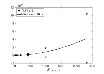
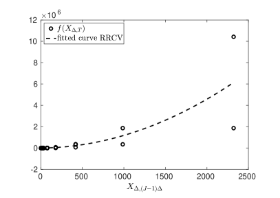
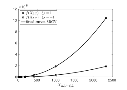
The latter property implies the absence of the statistical error while approximating $h_{j,y}.$ This is well illustrated by the first three plots in Figure 1 (the plots are performed for the example of Section 4.1).

2.3 RCV, RRCV and SRCV algorithms for second order schemes

Let us define the index set

$$\mathcal{I}=\left\{(k,l)\in\{1,\ldots,m\}^{2}:k<l\right\}$$

and consider a weak scheme of order $2$, where $d$-dimensional approximations $X_{\Delta,j\Delta}$, $j=0,\ldots,J$, satisfy $X_{\Delta,0}=x_{0}$ and

$$X_{\Delta,j\Delta}=\Phi_{\Delta}(X_{\Delta,(j-1)\Delta},\xi_{j},V_{j}),\quad j=1,\ldots,J,$$ (18)

for some functions $\Phi_{\Delta}\colon\mathbb R^{d+m+m(m-1)/2}\to\mathbb R^{d}$. Here,

• $\xi_{j}=(\xi_{j}^{k})_{k=1}^{m}$, $j=1,\ldots,J$, are $m$-dimensional random vectors with i.i.d.coordinates satisfying

  $$\mathbb P\left(\xi_{j}^{k}=\pm\sqrt{3}\right)=\frac{1}{6},\quad\mathbb P\left(\xi_{j}^{k}=0\right)=\frac{2}{3},$$

• $V_{j}=(V_{j}^{kl})_{(k,l)\in\mathcal{I}}$, $j=1,\ldots,J$, are $m(m-1)/2$-dimensional random vectors with i.i.d. coordinates satisfying

  $$\mathbb P\left(V_{j}^{kl}=\pm 1\right)=\frac{1}{2},$$

• the pairs $(\xi_{j},V_{j})$, $j=1,\ldots,J$, are independent,

• for each $j$, the random vectors $\xi_{j}$ and $V_{j}$ are independent.

An important example of such a scheme is the simplified order $2$ weak Taylor scheme in Section 14.2 of [4], which has the discretisation error $\mathbb E[f(X_{T})]-\mathbb E[f(X_{\Delta,T})]$ of order $\Delta^{2}$ under appropriate conditions on $f$, $\mu$ and $\sigma$ (also see Theorem 2.1 in [5]). Let us introduce the notation

$$\mathcal{U}=\left\{(o,r)\in\{0,1,2\}^{m}\times\{0,1\}^{\mathcal{I}}:o_{i}\neq 0\text{ for some }i\text{ or }r_{kl}\neq 0\text{ for some }k,\;l\right\},$$

where $o_{i}$, $i=1,\ldots,m$ (resp. $r_{kl}$, $(k,l)\in\mathcal{I}$), denote the coordinates of $o$ (resp. $r$). The following result is an equivalent reformulation of Theorem 3.5 in [1].

Theorem 2

The following representation holds

$$f(X_{\Delta,T})=\mathbb Ef(X_{\Delta,T})+\sum_{j=1}^{J}\sum_{(o,r)\in\mathcal{U}}a_{j,o,r}(X_{\Delta,(j-1)\Delta})\prod_{i=1}^{m}H_{o_{i}}(\xi_{j}^{i})\prod_{(k,l)\in\mathcal{I}}(V_{j}^{kl})^{r_{kl}},$$ (19)

where $H_{0}(x):=1$, $H_{1}(x):=x$, $H_{2}(x):=\frac{x^{2}-1}{\sqrt{2}}$, and the coefficients $a_{j,o,r}\colon\mathbb R^{d}\to\mathbb R$ are given by the formula

$$a_{j,o,r}(x)=\mathbb E\left[\left.f(X_{\Delta,T})\prod_{i=1}^{m}H_{o_{i}}(\xi_{j}^{i})\prod_{(k,l)\in\mathcal{I}}(V_{j}^{kl})^{r_{kl}}\right|X_{\Delta,(j-1)\Delta}=x\right]$$ (20)

for all $j\in\{1,\ldots,J\}$ and $(o,r)\in\mathcal{U}$.

Thus, with

$$M^{(2)}_{\Delta,T}:=\sum_{j=1}^{J}\sum_{(o,r)\in\mathcal{U}}a_{j,o,r}(X_{\Delta,(j-1)\Delta})\prod_{i=1}^{m}H_{o_{i}}(\xi_{j}^{i})\prod_{(k,l)\in\mathcal{I}}(V_{j}^{kl})^{r_{kl}},$$ (21)

we have $\mathbb E\left[M^{(2)}_{\Delta,T}\right]=0$ and $\operatorname{Var}\left[f(X_{\Delta,T})-M^{(2)}_{\Delta,T}\right]=0$ in the case of second order schemes. The RCV approach for second order schemes relies on Theorem 2 in the same way as the one for first order schemes relies on Theorem 1.

We now introduce the functions $q_{j}(x)$, $j\in\{1,\ldots,J\}$, by formula (9) also in the case of second order schemes and, for all $y\in\{-\sqrt{3},0,\sqrt{3}\}^{m}$, set

$$p_{m}(y):=\frac{4^{\sum_{i=1}^{m}I(y_{i}=0)}}{6^{m}2^{\frac{m(m-1)}{2}}}.$$ (22)

Notice that $p_{m}(y)=\mathbb P(\xi_{j}=y,V_{j}=z)$ for all $z\in\{-1,1\}^{\mathcal{I}}$. The next result is Proposition 3.7 of [1].

Proposition 2

We have $q_{J}\equiv f$ and, for each $j\in\{2,\ldots,J\}$,

$$q_{j-1}(x)= \mathbb E\bigl{[}q_{j}(X_{\Delta,j\Delta})|X_{\Delta,(j-1)\Delta}=x\bigr{]}=\!\!\!\!\sum_{y\in\{-\sqrt{3},0,\sqrt{3}\}^{m}}\;\sum_{z\in\{-1,1\}^{\mathcal{I}}}p_{m}(y)\,q_{j}(\Phi_{\Delta}(x,y,z)).$$ (23)

Moreover, for all $j\in\{1,\ldots,J\}$ and $(o,r)\in\mathcal{U}$, the functions $a_{j,o,r}(x)$ of (20) can be expressed in terms of the functions $q_{j}(x)$ as

$$a_{j,o,r}(x)=\!\!\!\!\sum_{y\in\{-\sqrt{3},0,\sqrt{3}\}^{m}}\;\sum_{z\in\{-1,1\}^{\mathcal{I}}}\left[p_{m}(y)\prod_{i=1}^{m}H_{o_{i}}(y_{i})\prod_{(k,l)\in\mathcal{I}}z_{kl}^{r_{kl}}\right]q_{j}(\Phi_{\Delta}(x,y,z)),$$ (24)

where $o_{i}$ and $y_{i}$, $i=1,\ldots,m$, denote the coordinates of $o$ and $y$, while $r_{kl}$ and $z_{kl}$, $(k,l)\in\mathcal{I}$, are the coordinates of $r$ and $z$.

Similar to (12), we define functions $h_{j,y,z}$, for all $j\in\{1,\ldots,J\}$, $y\in\{-\sqrt{3},0,\sqrt{3}\}^{m}$ and $z\in\{-1,1\}^{\mathcal{I}}$, by the formula

$$h_{j,y,z}(x):=q_{j}(\Phi_{\Delta}(x,y,z))=\mathbb E[q_{j}(X_{\Delta,j\Delta})|X_{\Delta,(j-1)\Delta}=x,\xi_{j}=y,V_{j}=z].$$ (25)

The RRCV and SRCV algorithms for second order schemes now rely on Proposition 2 and on (25) in the same way as the ones for first order schemes rely on Proposition 1 and on (12). The whole discussion in the end of Section 2.2, and, in particular, the formula $JK\max\{KN,(c_{m}-1)N_{0}\}$ for the overall cost order of the SRCV algorithm, apply also in the case of second order schemes, where we only need to change the value of $c_{m}$: here $c_{m}:=3^{m}2^{m(m-1)/2}$.

3 Complexity analysis

In this section we extend the complexity analysis presented in [1] to the case of the stratified regression algorithm. Below we only sketch the main results for the second order schemes. We make the following assumptions.

• All functions $h_{j,y,z}(x)$ of (25) are uniformly bounded, i.e. there is a constant $A>0$ such that $\sup_{x\in\mathbb R^{d}}|h_{j,y,z}(x)|\leq A<\infty$.

• The functions $h_{j,y,z}\left(x\right)$ can be well approximated by the functions from $\Psi_{K}:=\text{span}\left(\left\{\psi_{1},\ldots,\psi_{K}\right\}\right)$, in the sense that there are constants $\kappa>0$ and $C_{\kappa}>0$ such that

  $$\inf_{g\in\Psi_{K}}\int_{\mathbb{R}^{d}}\left(h_{j,y,z}\left(x\right)-g\left(x\right)\right)^{2}\,\mathbb P_{\Delta,j-1}(dx)\leq\frac{C_{\kappa}}{K^{\kappa}},$$

  where $\mathbb P_{\Delta,j-1}$ denotes the distribution of $X_{\Delta,(j-1)\Delta}$.

Remark 1

A sufficient condition for (A1) is boundedness of $f$. As for (A2), this is a natural condition to be satisfied for good choices of $\Psi_{K}$. For instance, under appropriate assumptions, in the case of piecewise polynomial regression as described in [1], (A2) is satisfied with $\kappa=\frac{2\nu(p+1)}{2d(p+1)+d\nu}$, where the parameters $p$ and $\nu$ are explained in [1].

In Lemma 1 below we present an $L^{2}$-upper bound for the estimation error on step 2 of the training phase of the SRCV algorithm (see page 2.2). To this end, we need to describe more precisely, how exactly the regression-based approximations $\tilde{h}_{j,y,z}$ are constructed:

• Let functions $\hat{h}_{j,y,z}(x)$ be obtained by linear regression (based on the second equality in (25)) onto the set of basis functions $\left\{\psi_{1},\ldots,\psi_{K}\right\}$, while the approximations $\tilde{h}_{j,y,z}(x)$ on step 2 of the training phase of the SRCV algorithm be the truncated estimates, which are defined as follows:

  $$\tilde{h}_{j,y,z}(x):=T_{A}\hat{h}_{j,y,z}(x):=\begin{cases}\hat{h}_{j,y,z}(x)&\text{if }|\hat{h}_{j,y,z}(x)|\leq A,\\ A\operatorname{sgn}\hat{h}_{j,y,z}(x)&\text{otherwise}\end{cases}$$

  ($A$ is the constant from (A1)).

Lemma 1

Under (A1)–(A3), we have

$$\mathbb{E}\|\tilde{h}_{j,y,z}-h_{j,y,z}\|^{2}_{L^{2}(\mathbb P_{\Delta,j-1})}\leq\tilde{c}\,A^{2}(\log N+1)\frac{K}{Np_{m}(y)}+\frac{8\,C_{\kappa}}{K^{\kappa}},$$ (26)

where $\tilde{c}$ is a universal constant and $p_{m}(y)$ is given in (22).

It is necessary to explain once in detail how to understand the left-hand side of (26). The functions $\hat{h}_{j,y,z}(x)$ (see (A3)) are linear combinations $\alpha_{1}\psi_{1}(x)+\ldots+\alpha_{K}\psi_{K}(x)$ of the basis functions, where the coefficients $\alpha_{i}$ are random in that they depend on the simulated training paths. That is, we have, in fact, $\hat{h}_{j,y,z}(x)=\hat{h}_{j,y,z}(x,D_{N}^{tr})$ and, consequently, $\tilde{h}_{j,y,z}(x)=\tilde{h}_{j,y,z}(x,D_{N}^{tr})$ (cf. (14)). Thus, the expectation in the left-hand side of (26) means averaging over the randomness in $D_{N}^{tr}$.

The next step is to provide an upper bound for the regression-based estimates of the coefficients $a_{j,o,r}$, which are constructed on step 3 of the training phase of the SRCV algorithm.

Lemma 2

Under (A1)–(A3), we have

$$\mathbb{E}\|\tilde{a}_{j,o,r}-a_{j,o,r}\|^{2}_{L^{2}(\mathbb P_{\Delta,j-1})}\leq c_{m}\tilde{c}\,A^{2}(\log N+1)\frac{K}{N}+\frac{8\,C_{\kappa}}{K^{\kappa}}C_{m,o},$$ (27)

where $C_{m,o}:=\sum_{y\in\{-\sqrt{3},0,\sqrt{3}\}^{m}}\;c_{m}2^{\frac{m(m-1)}{2}}\left[p_{m}(y)\prod_{i=1}^{m}H_{o_{i}}(y_{i})\right]^{2}$.

Let $(X_{\Delta,j\Delta})_{j=0,\ldots,J}$ be a testing path, which is independent of the training paths $D_{N}^{tr}$. We now define

$$\tilde{M}^{(2)}_{\Delta,T}:=\sum_{j=1}^{J}\sum_{(o,r)\in\mathcal{U}}\tilde{a}_{j,o,r}(X_{\Delta,(j-1)\Delta},D_{N}^{tr})\prod_{i=1}^{m}H_{o_{i}}(\xi_{j}^{i})\prod_{(k,l)\in\mathcal{I}}(V_{j}^{kl})^{r_{kl}}$$ (28)

(cf. (21)) and bound the variance $\operatorname{Var}[f(X_{\Delta,T})-\tilde{M}_{\Delta,T}^{(2)}]$ from above. With the help of Lemmas 1 and 2 we now derive the main result of this section:

Theorem 3

Under (A1)–(A3), it holds

$$\operatorname{Var}[f(X_{\Delta,T})-\tilde{M}^{(2)}_{\Delta,T}]\leq J\left(\left(c_{m}-1\right)c_{m}\tilde{c}\,A^{2}(\log N+1)\frac{K}{N}+\frac{8\,C_{\kappa}}{K^{\kappa}}\tilde{c}_{m}\right),$$

where $\tilde{c}_{m}=c_{m}-\left(\frac{3}{2}\right)^{m}$.

The preceding theorem allows us to perform complexity analysis for the SRCV approach, which means that we want to find the minimal order of the overall computational cost necessary to implement the algorithm under the constraint that the mean squared error is of order $\varepsilon^{2}$. The overall cost is of order $JK\max\left\{NK,(c_{m}-1)N_{0}\right\}$. We have the constraint

$$\mathbb E\left[\left(V_{N_{0}}^{SRCV}-\mathbb Ef(X_{T})\right)^{2}\right]\lesssim\varepsilon^{2},$$ (29)

where

$$V_{N_{0}}^{SRCV}:=\frac{1}{N_{0}}\sum_{i=1}^{N_{0}}\left[f\Bigl{(}X_{\Delta,T}^{(i)}\Bigr{)}-\tilde{M}_{\Delta,T}^{(2),(i)}\right].$$

Since

$$\mathbb E\left[\left(V_{N_{0}}^{SRCV}-\mathbb Ef(X_{T})\right)^{2}\right]=\left(\mathbb Ef(X_{\Delta,T})-\mathbb Ef(X_{T})\right)^{2}+\frac{1}{N_{0}}\operatorname{Var}\left[f(X_{\Delta,T})-\tilde{M}_{\Delta,T}^{(2)}\right],$$ (30)

constraint (29) reduces to

$$\max\left\{\frac{1}{J^{4}},\frac{JK\log(N)c_{m}(c_{m}-1)}{NN_{0}},\frac{JC_{\kappa}\tilde{c}_{m}}{K^{\kappa}N_{0}}\right\}\lesssim\varepsilon^{2},$$

where the first term comes from the squared bias of the estimator (see the first term in the right-hand side of (30)) and the remaining two ones come from the variance of the estimator (see the second term in the right-hand side of (30) and apply Theorem 3). It is natural to expect that the optimal solution is given by all constraints being active as well as $NK\asymp(c_{m}-1)N_{0}$, that is, both terms in the overall cost are of the same order. Provided that $\kappa>1$, we obtain the following parameter values:

$$J\asymp\varepsilon^{-\frac{1}{2}},\quad K\asymp\left[\frac{\tilde{c}_{m}^{2}C_{\kappa}^{2}}{c_{m}\varepsilon^{\frac{5}{2}}}\right]^{\frac{1}{2\kappa+2}},\quad N\asymp\frac{(c_{m}-1)\sqrt{c_{m}}}{\varepsilon^{\frac{5}{4}}}\sqrt{\log\left(\varepsilon^{-\frac{5}{4}}\right)},$$

$$N_{0}\asymp\frac{NK}{c_{m}-1}\asymp\left[\frac{c_{m}^{\kappa}\tilde{c}_{m}^{2}C_{\kappa}^{2}}{\varepsilon^{\frac{5\kappa+10}{2}}}\right]^{\frac{1}{2\kappa+2}}\sqrt{\log\left(\varepsilon^{-\frac{5}{4}}\right)}.$$

Thus, we have for the complexity

$$\mathcal{C} \asymp JNK^{2}\asymp JN_{0}K(c_{m}-1)\asymp\left[\frac{(c_{m}-1)^{2\kappa+2}c_{m}^{\kappa-1}\tilde{c}_{m}^{4}C_{\kappa}^{4}}{\varepsilon^{\frac{7\kappa+17}{2}}}\right]^{\frac{1}{2\kappa+2}}\sqrt{\log\left(\varepsilon^{-\frac{5}{4}}\right)}.$$ (31)

Note that the $\log$-term in the solution of $N$ and $N_{0}$ has been added afterwards to satisfy all constraints. Complexity estimate (31) shows that one can go beyond the complexity order $\varepsilon^{-2}$, provided that $\kappa>9$, and that we can achieve the complexity order $\varepsilon^{-1.75-\delta}$, for arbitrarily small $\delta>0$, provided $\kappa$ is large enough.

4 Numerical results

In this section, we present several numerical examples showing the efficiency of the SRCV approach. It turns that even the weak Euler scheme (5) already shows the advantage of the new methodology over the standard Monte Carlo (SMC) as well as over the original RCV and RRCV approaches in terms of variance reduction effect. Regarding the choice of basis functions, we use for the RCV, RRCV and SRCV approaches polynomials of degree $\leq p$, that is, $\psi_{l}(x)=\prod_{i=1}^{d}x_{i}^{l_{i}}$, where $l=(l_{1},\ldots l_{d})\in\left\{0,1,\ldots,p\right\}^{d}$ and $\sum_{l=1}^{d}l_{i}\leq p$. In addition to the polynomials, we consider the function $f$ as a basis function. We choose $J=100$, $N=10^{5}$, $N_{0}=10^{7}$, $p=1$ in all examples. Hence, we have overall $K=\binom{p+d}{d}+1=d+2$ basis functions in each regression. Then we compute the estimated variances for the SMC, RCV, RRCV and SRCV approaches. More precisely, when speaking about “variance” below (e.g. in Tables 1, 2 and 3) we mean sample variance of one summand $f(X_{\Delta,T}^{(i)})-\tilde{M}_{\Delta,T}^{(1),(i)}$ (see (15)) in the case of RCV, RRCV and SRCV, while, in the case of SMC, the sample variance of $f(X_{\Delta,T}^{(i)})$ is meant. Thus, we analyse the variance reduction effect only, since the bias is the same for all these methods. To measure the numerical performance of a variance reduction method, we look at the ratio of variance vs. computational time, i.e., for the SRCV, we look at

$$\theta_{\text{SRCV}}:=\frac{\textrm{Var}_{\text{SRCV}}}{\textrm{Var}_{\text{SMC}}}\cdot\frac{\textrm{Time}_{\text{SRCV}}}{\textrm{Time}_{\text{SMC}}},$$

where $\textrm{Var}_{\text{SRCV}}$ and $\textrm{Time}_{\text{SRCV}}$ denote the variance and the overall computational time of the SRCV approach ($\textrm{Var}_{\text{SMC}}$ and $\textrm{Time}_{\text{SMC}}$ have the similar meaning). The smaller $\theta_{\text{SRCV}}$ is, the more profitable is the SRCV algorithm compared to the SMC one. We similarly define $\theta_{\text{RCV}}$ and $\theta_{\text{RRCV}}$ (each of the regression-based algorithms is compared with the SMC approach).

4.1 Geometric Brownian motion (GBM) with high volatility

Here $d=m=1$ ($K=3$). We consider the following SDE

$$dX_{t}= rX_{t}dt+\sigma X_{t}dW_{t},\quad X_{0}=1,$$ (32)

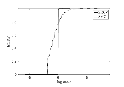
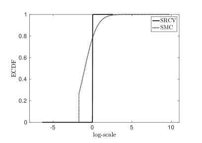
for $t\in\left[0,1\right]$, where $r=-1$ and $\sigma=4$. Furthermore, we consider the functional $f(x)=x^{2}$. In the following, we plot the empirical cumulative distribution function (ECDF) of the “log-scaled sample”, which is

$$\log(1+f_{i}-f_{\min})-\log(1+\bar{f}-f_{\min})$$

for the SMC, and

$$\log(1+u_{i}-u_{\min})-\log(1+\bar{u}-u_{\min})$$

for the RCV, and RRCV and SRCV, where

$$f_{i} :=f(X_{\Delta,T}^{(i)}),\quad u_{i}:=f_{i}-\tilde{M}_{\Delta,T}^{(1),(i)},\quad i\in\left\{1,\ldots,N_{0}\right\},$$

$$f_{\min} :=\min_{i=1,\ldots,N_{0}}f_{i},\quad u_{\min}:=\min_{i=1,\ldots,N_{0}}u_{i},\quad\bar{f}:=\frac{1}{N_{0}}\sum_{i=1}^{N_{0}}f_{i},\quad\bar{u}:=\frac{1}{N_{0}}\sum_{i=1}^{N_{0}}u_{i}.$$

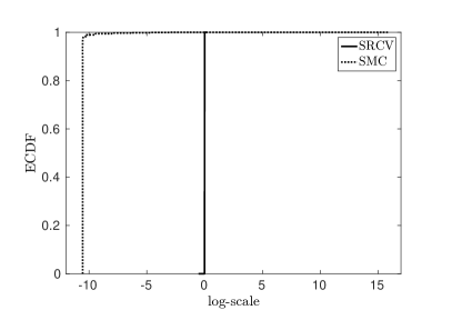
The results for such a log-scaled sample are illustrated in Table 1. As can be also seen from the fourth plot in Figure 1 (ECDFs of the SRCV and SMC), the variance reduction works absolutely fine for SRCV. Most of the sample values produced by SMC are much smaller than the corresponding mean value, whereas the deviation w.r.t. the mean $\bar{u}$ is very small for the SRCV approach. The main problem of the SMC approach in this case is that almost all paths tend to zero so that the small number of outliers is not sufficient to reach the (large) expectation $\mathbb E[f(X_{\Delta,T})]$, i.e. $N_{0}$ has to be increased a lot to approach the expectation. In contrast, for the SRCV approach all paths (paths close to zero as well as outliers) are “shifted” close to the expectation and thus we obtain a very small variance. We only plot the ECDFs of the SRCV and SMC in Figure 1, since the ECDFs of the RCV and RRCV look visually very similar to that for SRCV. The difference is, however, revealed in the “Min” and “Max” columns of the Table 1. That is, the RCV and RRCV algorithms produce several outliers which result in that the RCV and RRCV do not give us any variance reduction effect! One reason for this significant difference between the algorithms is given in the first three plots in Figure 1, where we illustrate the regression results for the RCV, RRCV and SRCV algorithms at the last time point, which means the first regression task. Here, we have accurate estimates only for the SRCV (cf. the discussion around (17)).

Approach	Min	Max	Variance	Time (sec)	$\theta$
SRCV	-0.5	0.2	$6.3\cdot 10^{-8}$	30.5	$1.32\cdot 10^{-23}$
RRCV	-25.4	1.7	$2.7\cdot 10^{16}$	65.3	12.38
RCV	-27.8	0.1	$1.4\cdot 10^{17}$	30.0	28.57
SMC	-10.6	15.9	$9.6\cdot 10^{15}$	15.1	1

Table 1: Results of the algorithms for a quadratic function $f$ under a GBM model.

4.2 High-dimensional geometric Brownian motion

We consider the following SDE for $d=m=10$ ($K=12$):

$$dX_{t}^{i}=rX_{t}^{i}dt+\sigma^{i}X_{t}^{i}A^{i}dW_{t},\quad t\in\left[0,1\right],\quad i=1,\ldots,10,$$

where $X_{0}^{i}=1$, $\sigma^{i}=2\,\forall i,$ $r=0.05$ and $A^{i}:=\begin{pmatrix}A^{i,1}\cdots A^{i,10}\end{pmatrix}$, $AA^{T}=\left(\rho_{ik}\right)_{i,k=1,\ldots,10}$ with $\rho_{ik}=\rho_{ki}\in\left[-1,1\right]$ and $\rho_{ik}=1$ for $i=k$ (that is, $A^{i}W$, $i=1,\ldots,10$, are correlated Brownian motions). For $i<k$ we choose

$$\rho_{ik}=\left\{\begin{array}[]{lllrll}0.9&\text{if }i=1,\,k=2,&&-0.95&\text{if }i=3,\,k=4,\\ 0.5&\text{if }i=5,\,k=6,&&-0.9&\text{if }i=7,\,k=8,\\ 0.8&\text{if }i=9,\,k=10,&&0&\text{otherwise}.\end{array}\right.$$

In this example, we illustrate the performances of the algorithms by means of the functional $f\left(x\right)=\max\left\{\max_{i\in\left\{1,\ldots,10\right\}}x^{i}-1,0\right\}$. For saving a lot of computing time, we use the “simplified control variate”

$$\tilde{\tilde{M}}^{(1)}_{\Delta,T}:=\sum_{j=1}^{J}\sum_{r=1}^{m}\tilde{a}_{j,r}(X_{\Delta,(j-1)\Delta},D_{N}^{tr})\xi_{j}^{r}$$

rather than $\tilde{M}_{\Delta,T}^{(1)}$ for RCV and SRCV, where $\tilde{a}_{j,r}$ is a shorthand notation for $\tilde{a}_{j,k(r)}$ with $k(r)=(k_{1},\ldots,k_{m})$, $k_{r}=1$, $k_{i}=0$ for $i\neq r$. This simplification already takes much of the variance reduction power into account, while significantly reduces the number of summands needed to construct the control variate ($m=10$ vs. $c_{m}-1=2^{m}-1=1023$ summands in the second sum above). For the SRCV algorithm, this results in the cost order $N_{0}JmK$ instead of $N_{0}J(c_{m}-1)K$ in the testing phase ($10^{11}$ vs. $10^{13}$ in this example). Such a reduction in computational time due to using $\tilde{\tilde{M}}^{(1)}_{\Delta,T}$ applies also to the RCV algorithm, but does not apply to the RRCV algorithm. Namely, with $\tilde{\tilde{M}}^{(1)}_{\Delta,T}$ the testing phase of the RRCV algorithm would now cost $N_{0}Jc_{m}K+N_{0}Jmc_{m}$ (in the second summand we now have the factor $m$ instead of $c_{m}-1$, cf. footnote 4 on page 4), which is still of order $10^{13}$ in the present example. Therefore, we do not consider the RRCV approach in this example. The results for the log-scaled sample are illustrated in Table 2. Again, the SRCV approach achieves a much smaller variance compared to the SMC and RCV (see the fifth plot in Figure 1).

Approach	Min	Max	Variance	Time (sec)	$\theta$
SRCV	-5.8	2.0	14.6	573.9	0.13
RCV	-10.4	0.7	11271.0	288.2	51.50
SMC	-1.9	7.2	448.9	140.5	1

Table 2: Results of the algorithms for a Call-on-max-option under a high-dimensional GBM.

4.3 High-dimensional Heston model

We consider the following SDE for $d=m=9$ ($K=11$):

$$dX_{t}^{i} =rX_{t}^{i}dt+\sigma^{i}X_{t}^{i}\sqrt{X_{t}^{9}}A^{i}dW_{t},\quad i=1,\ldots,8,$$

$$dX_{t}^{9} =\lambda\left(\bar{v}-X_{t}^{9}\right)dt+\eta\sqrt{X_{t}^{9}}A^{9}dW_{t},$$

where $t\in\left[0,1\right]$, $X_{0}^{i}=1$, $\sigma^{i}=1$ for $i=1,\ldots,8$ as well as $X_{0}^{9}=4$, $r=0.05$, $\lambda=0.1$, $\bar{v}=4$, $\eta=1$ and $A^{i}:=\begin{pmatrix}A^{i,1}\cdots A^{i,9}\end{pmatrix}$, $AA^{T}=\left(\rho_{ik}\right)_{i,k=1,\ldots,9}$. Here, for $i<k$ we choose

$$\rho_{ik}=\left\{\begin{array}[]{lllrll}0.9&\text{if }i=1,\,k=2,&&-0.95&\text{if }i=3,\,k=4,\\ 0.5&\text{if }i=5,\,k=6,&&-0.9&\text{if }i=7,\,k=8,\\ -0.2&\text{if }i\in\left\{1,2,3,5,6,7\right\},\,k=9,&&0.2&\text{if }i\in\left\{4,8\right\},\,k=9,\\ 0&\text{otherwise}.\end{array}\right.$$

One might think about $X^{1},\ldots,X^{8}$ as about price process of $8$ stocks, while the CIR process $X^{9}$ is their common stochastic volatility. Notice that Feller’s condition for $X^{9}$ is not satisfied ($\frac{2\lambda\bar{v}}{\eta^{2}}=0.8<1$), that is, $0$ is accessible boundary point for $X^{9}$ (with reflecting boundary behaviour). The discretised process $(X_{\Delta,j\Delta}^{9})_{j=0,\ldots,J}$ can become negative. We, therefore, use the following discretisation scheme

$$X^{i}_{\Delta,j\Delta} =X^{i}_{\Delta,(j-1)\Delta}\left(1+r\Delta+\sigma^{i}\sqrt{\left(X_{\Delta,(j-1)\Delta}^{9}\right)^{+}}A^{i}\sqrt{\Delta}\xi_{j}\right),$$

$$X^{9}_{\Delta,j\Delta} =X^{9}_{\Delta,(j-1)\Delta}+\lambda\left(\bar{v}-\left(X_{\Delta,(j-1)\Delta}^{9}\right)^{+}\right)\Delta+\eta\sqrt{\left(X_{\Delta,(j-1)\Delta}^{9}\right)^{+}}A^{9}\sqrt{\Delta}\xi_{j},$$

where $i\in\left\{1,\ldots,8\right\}$ and $x^{+}:=\max\left\{x,0\right\}$. Here, we consider of the functional $f\left(x\right)=\max\left\{\max_{i\in\left\{1,\ldots,8\right\}}x^{i}-1,0\right\}$ and, as in Section 4.2, use the simplified control variate $\tilde{\tilde{M}}_{\Delta,T}^{(1)}$ (we again exclude the RRCV approach). The results for the log-scaled sample are illustrated in Table 3. We get that the ECDF for the SRCV approach has a similar form as the one from Section 4.2 (see the sixth plot in Figure 1). Notice that the values of the estimators lie in all cases around 4.6 (SMC: 4.62, RCV: 4.59, SRCV: 4.60). Nevertheless, in the case of the SRCV approach $75.5\%$ of the paths are located within the interval $\left(3,6\right)$, whereas in case of the SMC approach this holds for only $13.0\%$ of the paths and in case of the RCV approach for only $9.9\%$. This is a further indication of a better numerical performance of the SRCV approach.

Approach	Min	Max	Variance	Time (sec)	$\theta$
SRCV	-6.4	2.6	50.1	444.7	0.09
RCV	-10.2	1.0	3208.8	328.6	4.33
SMC	-1.7	9.8	1478.8	164.5	1

Table 3: Results of the algorithms for a Call-on-max-option in a high-dimensional Heston model.

5 Proofs

5.1 Proof of Lemma 1

Applying Theorem 11.3 in [2] and using Assumption (A1) leads to

$$\mathbb{E}\|\tilde{h}_{j,y,z}-h_{j,y,z}\|^{2}_{L^{2}(\mathbb P_{\Delta,j-1})}$$

$$\leq \tilde{c}\,A^{2}(\log(Np_{m}(y))+1)\frac{K}{Np_{m}(y)}+8\inf_{g\in\Psi_{K}}\int_{\mathbb{R}^{d}}\left(h_{j,y,z}\left(x\right)-g\left(x\right)\right)^{2}\,\mathbb P_{\Delta,j-1}(dx),$$

since the expected number of (training) paths given $\xi_{j}=y,V_{j}=z$ is $Np_{m}(y)$ and

$$\operatorname{Var}[q_{j}(X_{\Delta,j\Delta})|X_{\Delta,(j-1)\Delta}=x,\xi_{j}=y,V_{j}=z]=\operatorname{Var}[q_{j}(\Phi_{\Delta}(x,y,z))]=0.$$

By means of Assumption (A2) and $\log p_{m}(y)<0$ we finally obtain (26).

5.2 Proof of Lemma 2

Let us first recall that $2^{m(m-1)/2}p_{m}(y)=\mathbb P(\xi_{j}=y)=\prod_{i=1}^{m}\mathbb P(\xi_{j}^{i}=y_{i})$ (cf. (22)). Lemma 1 together with formulas (24) and (26) as well as $(\sum_{i=1}^{c_{m}}b_{i})^{2}\leq c_{m}\sum_{i=1}^{c_{m}}b_{i}^{2}$ yield

$$\mathbb{E}\|\tilde{a}_{j,o,r}-a_{j,o,r}\|^{2}_{L^{2}(\mathbb P_{\Delta,j-1})}$$

$$\leq c_{m}\sum_{y\in\{-\sqrt{3},0,\sqrt{3}\}^{m}}\;\sum_{z\in\{-1,1\}^{\mathcal{I}}}\left[p_{m}(y)\prod_{i=1}^{m}H_{o_{i}}(y_{i})\prod_{(k,l)\in\mathcal{I}}z_{kl}^{r_{kl}}\right]^{2}\mathbb{E}\|\tilde{h}_{j,y,z}-h_{j,y,z}\|^{2}_{L^{2}(\mathbb P_{\Delta,j-1})}$$

$$\leq c_{m}2^{\frac{m(m-1)}{2}}\sum_{y\in\{-\sqrt{3},0,\sqrt{3}\}^{m}}\;\left[\prod_{i=1}^{m}H_{o_{i}}(y_{i})\right]^{2}\left(\tilde{c}\,A^{2}(\log N+1)\frac{Kp_{m}(y)}{N}+\frac{8\,C_{\kappa}p_{m}(y)^{2}}{K^{\kappa}}\right)$$

$$=c_{m}\tilde{c}\,A^{2}(\log N+1)\frac{K}{N}\mathbb{E}\left[\prod_{i=1}^{m}H_{o_{i}}(\xi_{j}^{i})\right]^{2}+\frac{8\,C_{\kappa}}{K^{\kappa}}\!\!\sum_{y\in\{-\sqrt{3},0,\sqrt{3}\}^{m}}\;c_{m}2^{\frac{m(m-1)}{2}}\left[p_{m}(y)\prod_{i=1}^{m}H_{o_{i}}(y_{i})\right]^{2}$$

$$=c_{m}\tilde{c}\,A^{2}(\log N+1)\frac{K}{N}+\frac{8\,C_{\kappa}}{K^{\kappa}}C_{m,o},$$

where in the last equality we used that $\xi_{j}^{1},\ldots,\xi_{j}^{m}$ are independent and all $H_{o_{i}}(\xi_{j}^{i})$ have unit $L^{2}$-norm.

5.3 Proof of Theorem 3

It holds

$$\operatorname{Var}[f(X_{\Delta,T})-\tilde{M}_{\Delta,T}^{(2)}] =\operatorname{Var}[M_{\Delta,T}^{(2)}-\tilde{M}_{\Delta,T}^{(2)}]$$

$$=\mathbb E\operatorname{Var}[M_{\Delta,T}^{(2)}-\tilde{M}_{\Delta,T}^{(2)}|D_{N}^{tr}]+\operatorname{Var}\mathbb E[M_{\Delta,T}^{(2)}-\tilde{M}_{\Delta,T}^{(2)}|D_{N}^{tr}].$$

Due to the martingale transform structure in (21) and (28), we have

$$\mathbb E[M_{\Delta,T}^{(2)}-\tilde{M}_{\Delta,T}^{(2)}|D_{N}^{tr}]=0.$$

Together with the fact that the system $\left\{\prod_{i=1}^{m}H_{o_{i}}(\xi_{j}^{i})\prod_{(k,l)\in\mathcal{I}}(V_{j}^{kl})^{r_{kl}}:(o,r)\in\mathcal{U}\right\}$ is orthonormal in $L^{2}$, we get

$$\operatorname{Var}[f(X_{\Delta,T})-\tilde{M}_{\Delta,T}^{(2)}]=\sum_{j=1}^{J}\sum_{(o,r)\in\mathcal{U}}\mathbb{E}\|\tilde{a}_{j,o,r}-a_{j,o,r}\|^{2}_{L^{2}(\mathbb P_{\Delta,j-1})}.$$ (33)

With the expression $C_{m,o}$ of Lemma 2 we compute

$$\sum_{(o,r)\in\mathcal{U}}C_{m,o} =\sum_{o\in\{0,1,2\}^{m}}\sum_{r\in\{0,1\}^{\mathcal{I}}}C_{m,o}-\sum_{y\in\{-\sqrt{3},0,\sqrt{3}\}^{m}}\;c_{m}2^{\frac{m(m-1)}{2}}p_{m}(y)^{2}$$

$$=\sum_{o\in\{0,1,2\}^{m}}2^{\frac{m(m-1)}{2}}C_{m,o}-\sum_{y\in\{-\sqrt{3},0,\sqrt{3}\}^{m}}\;c_{m}2^{\frac{m(m-1)}{2}}p_{m}(y)^{2}$$

$$:=\alpha-\beta,$$

where $\alpha$ (resp. $\beta$) denotes the first (resp. second) big sum in the above expression. Let us compute $\alpha$ and $\beta$. Recalling that

$$2^{m(m-1)/2}p_{m}(y)=\mathbb P(\xi_{j}=y)=\prod_{i=1}^{m}\mathbb P(\xi_{j}^{i}=y_{i}),$$

we get

$$\alpha =c_{m}\sum_{o\in\{0,1,2\}^{m}}\sum_{y\in\{-\sqrt{3},0,\sqrt{3}\}^{m}}\;\prod_{i=1}^{m}\left[\mathbb P(\xi_{j}^{i}=y_{i})H_{o_{i}}(y_{i})\right]^{2}$$

$$=c_{m}\left(\sum_{o_{1}\in\{0,1,2\}}\sum_{y_{1}\in\{-\sqrt{3},0,\sqrt{3}\}}\left[\mathbb P(\xi_{j}^{1}=y_{1})H_{o_{1}}(y_{1})\right]^{2}\right)^{m}=c_{m},$$

where the last equality follows by a direct calculation. Recalling that $c_{m}=3^{m}2^{m(m-1)/2}$ (we consider second order schemes), we obtain

$$\beta=3^{m}\!\!\sum_{y\in\{-\sqrt{3},0,\sqrt{3}\}^{m}}\;\prod_{i=1}^{m}\mathbb P(\xi_{j}^{i}=y_{i})^{2}=3^{m}\left(\sum_{y_{1}\in\{-\sqrt{3},0,\sqrt{3}\}}\mathbb P(\xi_{j}^{1}=y_{1})^{2}\right)^{m}=\left(\frac{3}{2}\right)^{m}.$$

Thus,

$$\sum_{(o,r)\in\mathcal{U}}C_{m,o}=c_{m}-\left(\frac{3}{2}\right)^{m}=\tilde{c}_{m}.$$

The last expression together with Lemma 2 and (33) yield the result.

Figure 1:

1. top left: first regression task for RCV (Section 4.1),

2. top right: first regression task for RRCV (Section 4.1),

3. center left: first regression task for SRCV (Section 4.1),

4. center right: ECDF of the log-scaled sample for SRCV and SMC (Section 4.1),

5. bottom left: ECDF of the log-scaled sample for SRCV and SMC (Section 4.2),

6. bottom right: ECDF of the log-scaled sample for SRCV and SMC (Section 4.3).

References

- Belomestny et al. [2016] Belomestny, D., Häfner, S., Nagapetyan, T., Urusov, M., 2016. Variance reduction for discretised diffusions via regression. Preprint, arXiv:1510.03141v3 .
- Györfi et al. [2002] Györfi, L., Kohler, M., Krzyżak, A., Walk, H., 2002. A Distribution-free Theory Of Nonparametric Regression. Springer Series in Statistics, Springer-Verlag, New York. URL: http://dx.doi.org/10.1007/b97848, doi:10.1007/b97848.
- Heath and Platen [2002] Heath, D., Platen, E., 2002. A variance reduction technique based on integral representations. Quant. Finance 2, 362–369. URL: http://dx.doi.org/10.1088/1469-7688/2/5/305, doi:10.1088/1469-7688/2/5/305.
- Kloeden and Platen [1992] Kloeden, P.E., Platen, E., 1992. Numerical Solution Of Stochastic Differential Equations. volume 23 of Applications of Mathematics (New York). Springer-Verlag, Berlin. URL: http://dx.doi.org/10.1007/978-3-662-12616-5, doi:10.1007/978-3-662-12616-5.
- Milstein and Tretyakov [2004] Milstein, G.N., Tretyakov, M.V., 2004. Stochastic Numerics For Mathematical Physics. Scientific Computation, Springer-Verlag, Berlin. doi:10.1007/978-3-662-10063-9.
- Milstein and Tretyakov [2009] Milstein, G.N., Tretyakov, M.V., 2009. Practical variance reduction via regression for simulating diffusions. SIAM J. Numer. Anal. 47, 887–910. URL: http://dx.doi.org/10.1137/060674661, doi:10.1137/060674661.
- Newton [1994] Newton, N.J., 1994. Variance reduction for simulated diffusions. SIAM J. Appl. Math. 54, 1780–1805. URL: http://dx.doi.org/10.1137/S0036139992236220, doi:10.1137/S0036139992236220.
- Privault and Schoutens [2002] Privault, N., Schoutens, W., 2002. Discrete chaotic calculus and covariance identities. Stoch. Stoch. Rep. 72, 289–315. URL: http://dx.doi.org/10.1080/10451120290019230, doi:10.1080/10451120290019230.