Pan-STARRS Pixel Processing : Detrending, Warping, Stacking

Abstract

The Pan-STARRS1 Science Consortium has carried out a set of imaging surveys using the 1.4 gigapixel GPC1 camera on the PS1 telescope. As this camera is composed of many individual electronic readouts, and covers a very large field of view, great care was taken to ensure that the many instrumental effects were corrected to produce the most uniform detector response possible. We present the image detrending steps used as part of the processing of the data contained within the public release of the Pan-STARRS1 Data Release 1 (DR1). In addition to the single image processing, the methods used to transform the 375,573 individual exposures into a common sky-oriented grid are discussed, as well as those used to produce both the image stack and difference combination products.

1. Introduction

The 1.8m Pan-STARRS 1 telescope is located on the summit of Haleakala on the Hawaiian island of Maui. The wide-field optical design of the telescope (Hodapp et al., 2004) produces a 3.3 degree field of view with low distortion and minimal vignetting even at the edges of the illuminated region. The optics and natural seeing combine to yield good image quality: 75% of the images have full-width half-max values less than (1.51, 1.39, 1.34, 1.27, 1.21) arcseconds for ($g_{\rm P1}$,$r_{\rm P1}$,$i_{\rm P1}$,$z_{\rm P1}$,$y_{\rm P1}$), with a floor of $\sim 0.7$ arcseconds.

The Pan-STARRS 1 camera (Tonry & Onaka, 2009), known as GPC1, consists of a mosaic of 60 back-illuminated CCDs manufactured by Lincoln Laboratory. The CCDs each consist of an $8\times 8$ grid of $590\times 598$ pixel readout regions, yielding an effective $4846\times 4868$ detector. Initial performance assessments are presented in Onaka et al. (2008). Routine observations are conducted remotely from the Advanced Technology Research Center in Kula, the main facility of the University of Hawaii’s Institute for Astronomy (IfA) operations on Maui. The Pan-STARRS1 filters and photometric system have already been described in detail in Tonry et al. (2012).

For nearly 4 years, from 2010 May through 2014 March, this telescope was used to perform a collection of astronomical surveys under the aegis of the Pan-STARRS Science Consortium. The majority of the time (56%) was spent on surveying the $\frac{3}{4}$ of the sky north of $-30$ Declination with $g_{\rm P1}$,$r_{\rm P1}$,$i_{\rm P1}$,$z_{\rm P1}$,$y_{\rm P1}$ filters in the so-called $3\pi$ Survey. Another $\sim 25\%$ of the time was concentrated on repeated deep observations of 10 specific fields in the Medium-Deep Survey. The rest of the time was used for several other surveys, including a search for potentially hazardous asteroids in our solar system. The details of the telescope, surveys, and resulting science publications are described by Chambers et al. (2017). The Pan-STARRS1 filters and photometric system has already been described in detail in Tonry et al. (2012).

Pan-STARRS produced its first large-scale public data release, Data Release 1 (DR1) on 16 December 2016. DR1 contains the results of the third full reduction of the Pan-STARRS $3\pi$ Survey archival data, identified as PV3. Previous reductions (PV0, PV1, PV2; see Magnier et al., 2017) were used internally for pipeline optimization and the development of the initial photometric and astrometric reference catalog (Magnier et al., 2016a). The products from these reductions were not publicly released, but have been used to produce a wide range of scientific papers from the Pan-STARRS 1 Science Consortium members (Chambers et al., 2017). DR1 contained only average information resulting from the many individual images obtained by the $3\pi$ Survey observations. A second data release, DR2, was made available 28 January 2019. DR2 provides measurements from all of the individual exposures, and include an improved calibration of the PV3 processing of that dataset.

This is the third in a series of seven papers describing the Pan-STARRS1 Surveys, the data reduction techniques and the resulting data products. This paper (Paper III) describes the details of the pixel processing algorithms, including detrending, warping, adding (to create stacked images), and subtracting (to create difference images), along with the resulting image products and their properties.

Chambers et al. (2017, Paper I) provide an overview of the Pan-STARRS System, the design and execution of the Surveys, the resulting image and catalog data products, a discussion of the overall data quality and basic characteristics, and a brief summary of important results.

Magnier et al. (2017, Paper II) describe how the various data processing stages are organized and implemented in the Imaging Processing Pipeline (IPP), including details of the the processing database which is a critical element in the IPP infrastructure.

Magnier et al. (2016b, Paper IV) describe the details of the source detection and photometry, including point-spread-function and extended source fitting models, and the techniques for “forced” photometry measurements.

Magnier et al. (2016a, Paper V) describe the final calibration process, and the resulting photometric and astrometric quality.

Flewelling et al. (2016, Paper VI) describe the details of the resulting catalog data and its organization in the Pan-STARRS database.

Huber et al. (2017, Paper VII) describe the Medium Deep Survey in detail, including the unique issues and data products specific to that survey. The Medium Deep Survey is not part of Data Releases 1 or 2 and will be made available in a future data release.

2. Background

The Pan-STARRS 1 Science Survey used the 1.4 gigapixel GPC1 camera with the PS1 telescope on Haleakala Maui to image the sky north of $-30^{\circ}$ declination. The GPC1 camera is composed of 60 orthogonal transfer array (OTA) devices arranged in an $8\times{}8$ grid, excluding the four corners. Each of the 60 devices is itself an $8\times{}8$ grid of readout cells. The large number of cells parallelizes the readout process, reducing the overhead in each exposure. However, as a consequence, many calibration operations are needed to ensure the response is consistent across the entire seven square degree field of view.

The Pan-STARRS image processing pipeline (IPP) is described elsewhere (Magnier et al., 2017), but a short summary follows. The raw image data is stored on the processing cluster, with a database containing the metadata of exposure parameters. These raw images can be launched for the initial chip stage processing. This stage performs the image detrending (described below in section 3), as well as the single epoch photometry (Magnier et al., 2016b), in parallel on the individual OTA device data. Following the chip stage is the camera stage, in which the astrometry and photometry for the entire exposure is calibrated by matching the detections against a reference catalog. This stage also performs masking updates based on the now-known positions and brightnesses of stars that create dynamic features (see Section 3.6.2 below). The warp stage is the next to operate on the data, transforming the detector oriented chip stage images onto common sky oriented images that have fixed sky projections (Section 5). When all warp stage processing is done for a region of the sky, stack processing is performed (Section 6) to construct deeper, fully populated images from the set of warp images that cover that region of the sky. Transient features are identified in the diff stage, which takes input warp and/or stack data and performs image differencing (Section 7). Further photometry is performed in the staticsky and skycal stages, which add extended source fitting to the point source photometry of objects detected in the stack images, and again calibrate the results against a reference catalog. The fullforce stage takes the catalog output of the skycal stage, and uses the objects detected in that to perform forced photometry on the individual warp stage images. The details of these stages are provided in Magnier et al. (2016b).

A limited version of the same reduction procedure described above is also performed in real time on new exposures as they are observed by the telescope. This process is automatic, with new exposures being downloaded from the summit to the main IPP processing cluster at the Maui Research and Technology Center in Kihei, and registered into the processing database. New chip stage reductions are launched for science exposures, advancing processing upon completion through to the diff stage, skipping the additional stack and forced warp photometry stages. This automatic processing allows the ongoing solar system moving object search to identify candidates for follow up observations within 24 hours of the initial set of observations (Wainscoat et al., 2015).

Section 3 provides an overview of the detrending process that corrects the instrumental signatures of GPC1, with details of the construction of the reference detrend templates in Section 4. An analysis of the algorithms used to perform the warp (section 5), stack (section 6), and diff (section 7) stage transformations of the image data follows after the list of detrend steps. Finally, a discussion of the remaining issues and possible future improvements is presented in section 8.

As mentioned above, the GPC1 camera is composed of 60 orthogonal transfer array (OTA) devices arranged in an $8\times{}8$ grid, excluding the four corners. Each of the 60 devices is itself an $8\times{}8$ grid of readout cells consisting of $590\times 598$ pixels. We label the OTAs by their coordinate in the camera grid in the form ‘OTAXY’, where X and Y each range from 0 - 7, e.g., OTA12 would be the chip in the $(1,2)$ position of the grid. Similarly, we identify the cells as ‘xyXY’ where X and Y again each range from 0 - 7.

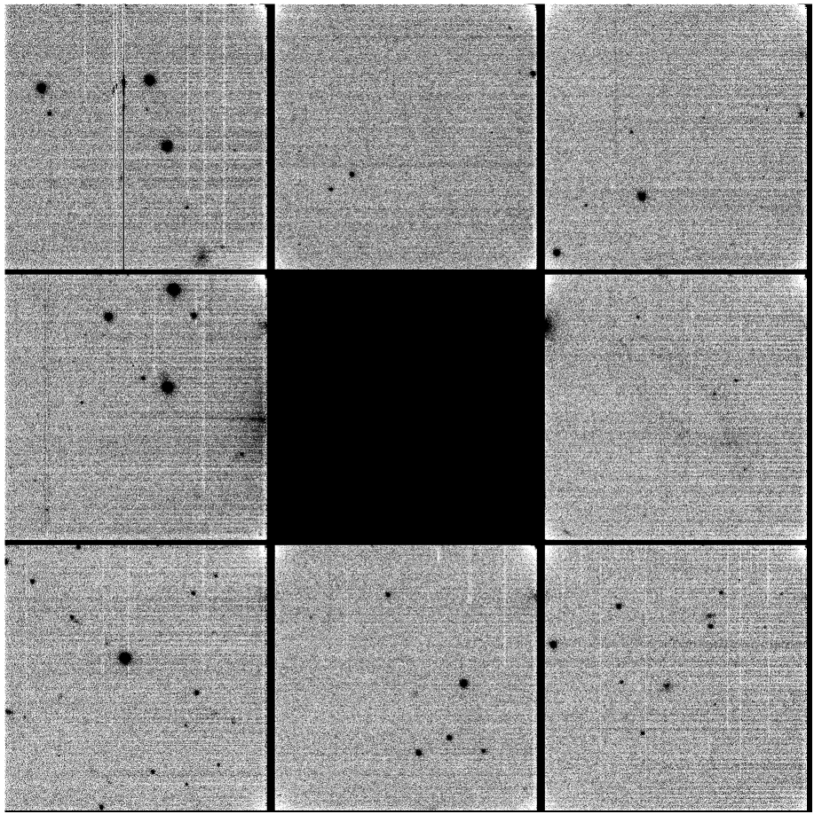
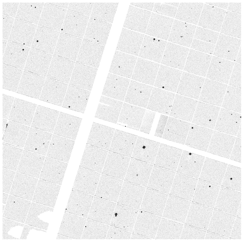
Image products presented in figures have been mosaicked to arrange pixels as follows. Single cell images are arranged such that pixel $(1,1)$ is at the lower right corner (for example Figure 9). This corrects the parity difference between the raw data and the sky. Images mosaicked to show a full OTA detector are arranged as they are on the focal plane (as in Figure 1. The OTAs to the left of the midplane (OTA4Y-OTA7Y) are oriented with cell xy00 and pixel $(590,1)$ to the lower right of their position. Due to the electronic connections of the OTAs in the focal plane, the OTAs to the right of the midplane (OTA0Y-OTA3Y) are rotated 180 degrees, and are oriented with cell xy00 and pixel $(590,1)$ to the top left of their position. For mosaics of the full field of view, the OTAs are arranged as they see the sky, with the cells arranged as in the single OTA images (Figure 6). The lower left corner is the empty location where OTA70 would exist. Toward the right, the OTA labels decrease in $X$ label, with the empty OTA00 located in the lower right. The OTA $Y$ labels increase upward in the mosaic.

3. GPC1 Detrend Details

Ensuring a consistent and uniform detector response across the three-degree diameter field of view of the GPC1 camera is essential to a well calibrated survey. Many standard image detrending steps are done for GPC1, with overscan subtraction removing the detector bias level, dark frame subtraction to remove temperature and exposure time dependent detector glows, and flat field correction to remove pixel to pixel response functions. We also perform fringe correction for the reddest data in the $y_{\rm P1}$ filter to remove the interference patterns that arise in that filter due to the variations in the thickness of the detector surface.

These corrections assume that the detector response is linear across the full dynamic range and that the pixels contain only signals coming from the imaged portion of the sky, or from linear dark current sources within the detector. This assumption is not universally true for GPC1, and an additional set of detrending steps are required as a result. The first of these is the burntool correction, which removes the flux trails left by the incomplete transfer of charge along the readout columns. These trails are generally only evident for the brightest stars, as only pixels that are at or beyond the saturation point of the detector leave residual charge. A second confounding effect is the non-linearity at the faint end of the pixel range. Some readout cells and some readout cell edge pixels experience a sag relative to the linear trend at low illumination, such that faint pixels appear fainter than expected. The correction to this requires amplifying the pixel values in these regions to match the linear response.

Large regions of some OTA cells experience significant charge transfer issues, making them unusable for science observations. These regions are therefore masked in processing, with these CTE regions making up the largest fraction of masked pixels on the detector. Other regions are masked for reasons such as static bad pixel features or temporary readout masking caused by issues in the camera electronics that make these regions unreliable. These all contribute to the detector mask, a 16 bit value which records the reason a pixel is masked based on the value added. This mask is augmented in each exposure for dynamic features that are masked based on the astronomical features within the field of view.

Within the IPP, all detrending is done by the ppImage program. This program applies the detrend corrections to the individual cells, and then an OTA-level mosaic is constructed for the signal image, the mask image, and the variance map image. The single epoch photometry is done at this stage as well. The following subsections (3.1 - 3.7) detail the detrending process used on GPC1 that are common to other detectors. The GPC1 specific detrending steps are included after, explaining these additional steps that remove the instrument signature.

3.1. Overscan

Each cell on GPC1 has an overscan region that covers the first 34 columns of each row, and the last 10 rows of each column. No light lands on these pixels, so the science region is trimmed to exclude them. Each row has an overscan value subtracted, calculated by finding the median value of that row’s overscan pixels and then smoothing between rows with a three-row boxcar median.

3.2. Dark/Bias Subtraction

Figure 1.— Dark Correction: An example of the dark model application to exposure o5677g0123o, OTA23 (2011-04-26, 43s $g_{\rm P1}$ filter). The left panel shows the image data mosaicked to the OTA level, and has had the static mask applied, the overscan subtracted, and the detector non-linearity corrected. The right panel, shows the same exposure with the dark applied in addition to the processing shown on the left, removing the amplifier glows in the cell corners.

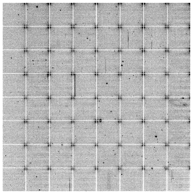
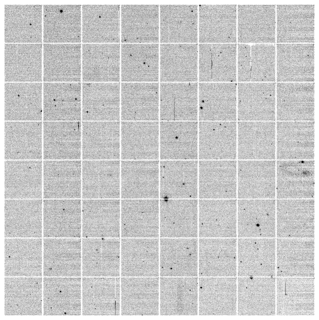
The dark current in the GPC1 detectors has significant variations across each cell. The model we make to remove this signal considers each pixel individually, independent of any neighbors. To construct this model, we fit a multi-dimensional model to the array of input pixels from a randomly selected set of 100-150 overscan and non-linearity corrected dark frames chosen from a given date range. The model fits each pixel as a function of the exposure time $t_{exp}$ and the detector temperature $T_{chip}$ of the input images such that $\mathrm{dark}=a_{0}+a_{1}t_{exp}+a_{2}T_{chip}t_{exp}+a_{3}T_{chip}^{2}t_{exp}$. This fitting uses two iterations to produce a clipped fit, rejecting at the $3\sigma$ level. The final coefficients $a_{i}$ for the dark model are stored in the detrend image. The constant $a_{0}$ term includes the residual bias signal after overscan subtraction, and as such, a separate bias subtraction is not necessary.

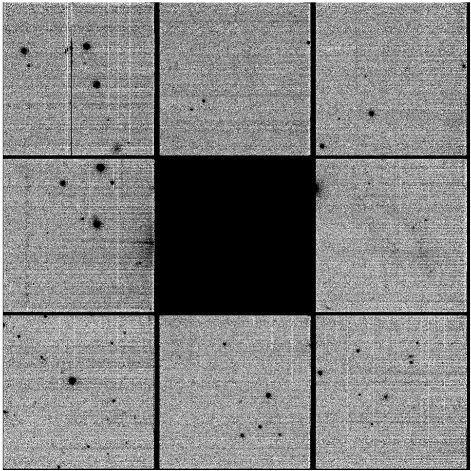
Applying the dark model is simply a matter of calculating the response for the exposure time and detector temperature of the image to be corrected, and subtracting the resulting dark signal from the image. Figure 1 shows the results of the dark subtraction.

3.2.1 Time evolution

Figure 2.— Example showing a profile cut across exposure o5676g0195, OTA67 (2011-04-25, 43s $g_{\rm P1}$ filter). The entire first row of cells (xy00-xy07) have had a median calculated along each pixel column on the OTA mosaicked image. Arbitrary offsets have been applied so the curves do not overlap. The top curve (in purple) shows the initial raw profile, with no dark model applied. The next curve (in green) shows the smoother profile after applying the appropriate B-mode dark model. Applying the (incorrect) A-mode dark instead results in the third (blue) curve, which shows a significant increase in gradients across the cells. The fourth (red) curve is the result of applying the PATTERN.CONTINUITY correction along with the B-mode dark model. Although this creates a larger gradient across the mosaicked images, it decreases the cell-to-cell boundary offsets. The bottom (black) curve shows the final image profile after all detrending and background subtraction (no offset applied). The bright source at the cell xy00 to xy01 transition is a result of a large optical ghost which, due to the area covered, increases the median level more than the field stars.

The dark model is not consistently stable over the full survey, with significant drift over the course of multiple months. Some of the changes in the dark can be attributed to changes in the voltage settings of the GPC1 controller electronics, but the causes of others are unknown. We can separate the dark model history of GPC1 into three epochs. The first epoch covers all data taken prior to 2010-01-23. This epoch used a different header keyword for the detector temperature, making data from this epoch incompatible with later dark models. In addition, the temperatures recorded in this value were not fully calibrated, making the dark model generated less reliable.

The second epoch covers data between 2010-01-23 and 2011-05-01, and is characterized by a largely stable but oscillatory dark solution. The dark model switches between two modes apparently at random. No clear cause has been established for the switching, but there are clear differences between the two modes that require the observation dates to be split to use the model that is most appropriate.

The initial evidence of these two modes comes from the discovery of a slight gradient along the rows of certain cells. This is a result of a drift in the bias level of the detector as it is read out. An appropriate dark model should remove this gradient entirely. For these two modes, the direction of this bias drift is different, so a single dark model generated from all dark images in the time range over corrects the positive-gradient mode, and under corrects the negative-gradient mode. Upon identifying this two-mode behavior, and determining the dates each mode was dominant, two separate dark models were constructed from appropriate “A” and “B” mode dark frames. Using the appropriate dark minimizes the effect of this bias gradient in the dark corrected data.

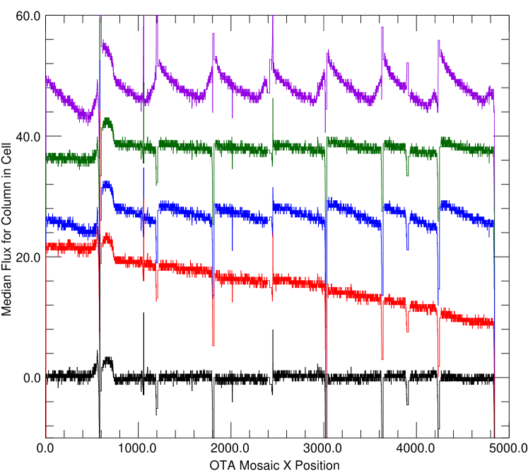
The bias drift gradients of the mode switching can be visualized in Figure 2. This figure shows the image profile along the x-pixel axis binned along the full y-axis of the first row of cells. The raw data is shown, illustrating the positional dependence the dark signal has on the image values. In addition, both the correct B-mode dark and incorrect A-mode dark have been applied to this image, showing that although both correct the bulk of the dark signal, using the incorrect mode creates larger intensity gradients.

After 2011-05-01, the two-mode behavior of the dark disappears, and is replaced with a slow observation-date-dependent drift in the magnitude of the gradient. This drift is sufficiently slow that we have modeled it by generating models for different date ranges. These darks cover the range from 2011-05-01 to 2011-08-01, 2011-08-01 to 2011-11-01, and 2011-11-01 and on. The reason for this time evolution is unknown, but as it is correctable with a small number of dark models, this does not significantly impact detrending.

3.2.2 Video Dark

Individual cells on GPC1 can be repeatedly read to create a video signal used for telescope guiding. However, when a cell is used for this purpose, the dark signal for the entire OTA is changed. The most noticeable feature of this change is that the glows in cell corners caused by the read-out amplifiers are suppressed. As a result, using the standard dark model on the data for these OTAs results in oversubtraction of the corner glow.

To generate a correction for this change, a set of video dark models were created by running the standard dark construction process on a series of dark frames that had the video signal enabled for some cells. GPC1 can only run video signals on a subset of the OTAs at a given time. This requires two passes to enable the video signal across the full set of OTAs that support video cells. This is convenient for the process of creating darks, as those OTAs that do not have video signals enabled create standard dark models, while the video dark is created for those that do.

This simultaneous construction of video and standard dark models is useful, as it provides a way to isolate the response on the standard dark from the video signals. If the standard and video dark signals are separable, then archival video darks can be constructed by applying the video dark response to the previously constructed dark models. Raw video dark frame data only exists after 2012-05-16, when this problem was initially identified, so any data prior to that can not be directly corrected for the video dark signal. Testing the separability shows that constructing a video dark for older data simply as $VD_{Old}=D_{Old}-D_{Modern}+VD_{Modern}$ produces a satisfactory result that does not over subtract the amplifier glow. This is shown in figure 3, which shows video cells from before 2012-05-16, corrected with both the standard and video darks, with the early video dark constructed in such a manner.

Figure 3.— Video Dark: An example of the video dark model application to exposure o5677g0123o, OTA22 (2011-04-26, 43s $g_{\rm P1}$ filter), which has a video cell located in cell xy16. The left panel shows the image data mosaicked to the OTA level, and has had the static mask applied, the overscan subtracted, the detector non-linearity corrected, and a regular dark applied. The right panel, shows the same exposure with a video dark applied instead of the standard dark. The main impact of this change is the improved correction of the corner glows, which are over subtracted with the standard dark.

3.3. Noisemap

Based on a study of the positional dependence of all detected sources, we discovered that the cells in GPC1 do not have uniform noise characteristics. Instead, there is a gradient along the pixel rows, with the noise generally higher away from the read out amplifier (higher cell $x$ pixel positions). This is likely an effect of the row-by-row bias issue discussed below (Section 3.10.1). As a result of this increased noise, more sources are detected in the higher noise regions when the read noise is assumed constant across the readout.

To mitigate this noise gradient, we constructed an initial set of noisemap images by measuring the median variance on bias frames processed as science images. The variance is calculated in boxes of 20x20 pixels, and then linearly interpolated to cover the full image.

Unfortunately, due to correlations within this noise, the variance measured from the bias images does not fully remove the positional dependence of objects that are detected. This simple noisemap underestimates the noise observed when the image is filtered during the object detection process. This filtering convolves the background noise with a PSF, which has the effect of amplifying the correlated peaks in the noise. This amplification can therefore boost background fluctuations above the threshold used to select real objects, contaminating the final object catalogs.

In the detection process, we expect false positives at a low rate, given that all sources are required to be significant at the $5\sigma$ level. Since the observed false positive rate was significantly higher than expected, we implemented an empirical “boost” to increase the noisemap to more accurately account for the position dependent read noise. By binning the number of false positives measured on the bias frames on the noisemap inputs using 20 pixel boxes in the cell $x$-axis, and comparing this to the number expected from random Gaussian noise, we estimated the true read noise level.

As the noisemap uses bias frames that have had a dark model subtracted, we constructed noisemaps for each dark model used for science processing. There is some evidence that the noise has changed over time as measured on full cells, so matching the noisemap to the dark model allows for these changes to be tracked. There is no evidence that the noisemap has the A/B modes found in the dark, so we do not generate separate models for that time period.

The noisemap detrend is not directly applied to the science image. Instead, it is used to construct the weight image that contains the pixel-by-pixel variance for the chip stage image. The initial weight image is constructed by dividing the science image by the cell gain (approximately 1.0 e${}^{-}/$ DN). This weight image contains the expected Poissonian variance in electrons measured. The square of the noisemap is then added to this initial weight, adding the additional empirical variance term in place of a single read noise value.

3.4. Flat

Determining a flat field correction for GPC1 is a challenging endeavor, as the wide field of view makes it difficult to construct a uniformly illuminated image. Using a dome screen is not possible, as the variations in illumination and screen rigidity create large scatter between different images that are not caused by the detector response function. Because of this, we use sky flat images taken at twilight, which are more consistently illuminated than screen flats. We calculate the mean of these images to determine the initial flat model.

From this starting skyflat model, we construct a photometric correction to remove the effect of the illumination differences over the detector surface. This is done by dithering a series of science exposures with a given pointing, as described in Magnier & Cuillandre (2004). By fully calibrating these exposures with the initial flat model, and then comparing the measured fluxes for the same star as a function of position on the detector, we can determine position dependent scaling factors. From the set of scaling factors for the full catalog of stars observed in the dithered sequence, we can construct a model of the error in the initial flat model as a function of detector position. Applying a correction that reduces the amplitude of these errors produces a flat field model that better represents the true detector response.

In addition to this flat field applied to the individual images, the “ubercal” analysis – in which photometric data are used define image zero points (Schlafly et al., 2012; Magnier et al., 2016a) and in turn used used to calibrate the database of all detections – constructs “in catalog” flat field corrections. Although a single set of image flat fields was used for the PV3 processing of the entire $3\pi$ survey, five separate “seasons” of database flat fields were needed to ensure proper calibration. This indicates that the flat field response is not completely fixed in time. More details on this process are contained in Magnier et al. (2016a).

3.5. Fringe correction

Due to variations in the thickness of the detectors, we observe interference patterns at the infrared end of the filter set, as the wavelength of the light becomes comparable to the thickness of the detectors. Visually inspecting the images shows that the fringing is most prevalent in the $y_{\rm P1}$ filter images, with negligible fringing in the other bands. As a result of this, we only apply a fringe correction to the $y_{\rm P1}$ filter data.

The fringe used for PV3 processing was constructed from a set of 20 120s science exposures. These exposures are overscan subtracted, and corrected for non-linearity, and have the dark and flat models applied. These images are smoothed with a Gaussian kernel with $\sigma=2$ pixels to minimize pixel to pixel noise. The fringe image data is then constructed by calculating the clipped mean of the input images with two iteration of clipping at the $3\sigma$ level.

A coarse background model for each cell is constructed by calculating the median on a 3x3 grid (approximately 200x200 pixels each). A set of 1000 points are randomly selected from the fringe image for each cell, and a median calculated for this position in a 10x10 pixel box, with the background level subtracted. These sample locations provide scale points to allow the amplitude of the measured fringe to be compared to that found on science images.

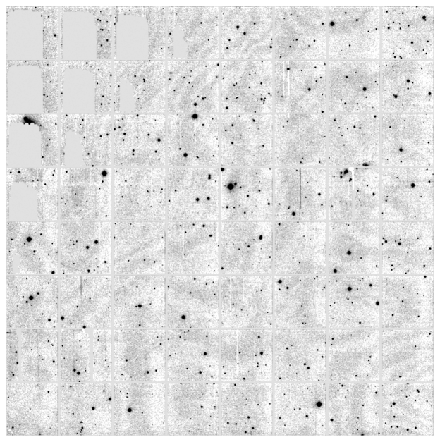
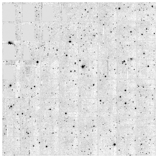
To apply the fringe, the same sample locations are measured on the science image to determine the relative strength of the fringing in that particular image. A least squares fit between the fringe measurements and the corresponding measurements on the science image provides the scale factor multiplied to the fringe before it is subtracted from the science image. An example of the fringe correction can be seen in Figure 4.

Figure 4.— Fringing: Example of the $y_{\rm P1}$ filter fringe pattern on exposure o5220g0025o OTA53 ($y_{\rm P1}$ filter 30s). The left panel shows the OTA mosaic with all detrending except the fringe correction, while the right shows the same including the fringe correction. Both images have been smoothed with a Gaussian with $\sigma=3$ pixels to highlight the faint and large scale fringe patterns.

3.6. Masking

3.6.1 Static Masks

Due to the large size of the detector, it is expected that there are a number of pixels that respond poorly. To remove these pixels, we have constructed a mask that identifies the known defects. This mask is referred to as the “static” mask, as it is applied to all images processed. The “dynamic” mask (Section 3.6.2) is calculated based on objects in the field, and so changes between images. Construction of the static mask consists of three phases.

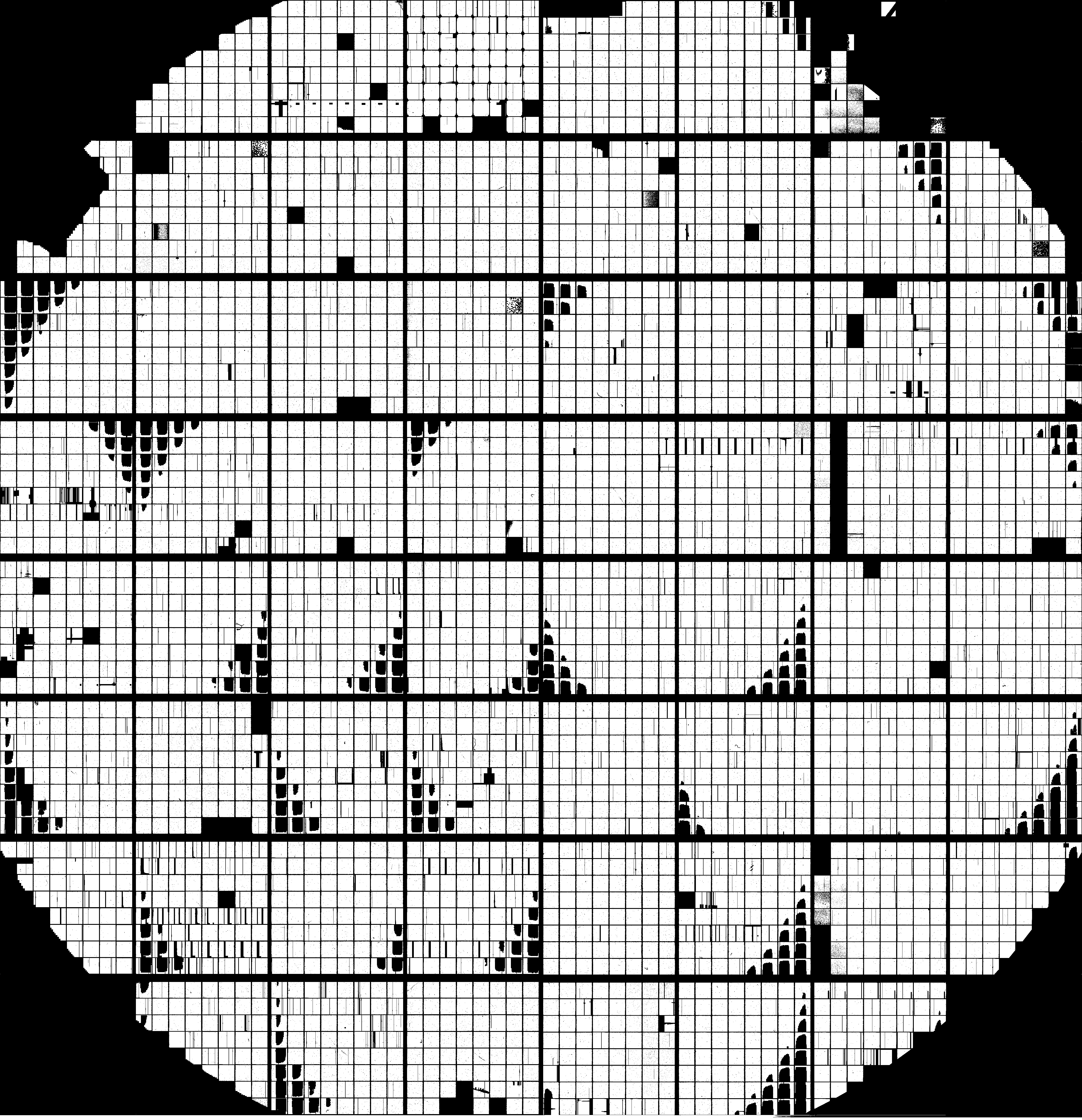
First, regions in which the charge transfer efficiency (CTE) is low compared to the rest of the detector are identified. Twenty-five of the sixty OTAs in GPC1 show some evidence of poor CTE, with this pattern appearing (to varying degrees) in roughly triangular patches. During the manufacture of the devices, an improperly tuned semiconductor process step resulted in a radial pattern of poor performance on some silicon wafers. When the OTAs were cut from these wafers, the outer corners exhibited the issue. To generate the mask for these regions, a sample set of 26 evenly-illuminated flat-field images were measured to produce a map of the image variance in 20x20 pixel bins. As the flat screen is expected to illuminate the image uniformly on this scale, the expected variances in each bin should be Poissonian distributed with the flux level. However, in regions with poor CTE, adjacent pixels are not independent, as the charge in those pixels is more free to spread along the image columns. This reduces the pixel-to-pixel differences, resulting in a lower than expected variance. All regions with variance less than half the average image level are added to the static mask.

The next step of mask construction is to examine the flat and dark models, and exclude pixels that appear to be poorly corrected by these models. The DARKMASK process looks for pixels that are more than $8\sigma$ discrepant in $10\%$ of the 100 input dark frame images after those images have had the dark model applied to them. These pixels are assumed to be unstable with respect to the dark model, and have the DARK bit set in the static mask, indicating that they are unreliable in scientific observing. Similarly, the FLATMASK process looks for pixels that are $3\sigma$ discrepant in the same fraction of 16 input flat field images after both the dark and flat models have been applied. Those pixels that do not follow the flat field model of the rest of image are assigned the FLAT mask bit in the static mask, removing the pixels that cannot be corrected to a linear response.

The final step of mask construction is to examine the detector for bright columns and other static pixel issues. This is first done by processing a set of 100 $i_{\rm P1}$ filter science images in the same fashion as for the DARKMASK. A median image is constructed from these inputs along with the per-pixel variance. These images are used to identify pixels that have unexpectedly low variation between all inputs, as well as those that significantly deviate from the global median value. Once this initial set of bad pixels is identified, a $3\times{}3$ pixel triangular kernel is convolved with the initial set, and any convolved pixel with value greater than 1 is assigned to the static mask. This does an excellent job of removing the majority of the problem pixels. A subsequent manual inspection allows human interaction to identify other inconsistent pixels including the vignetted regions around the edge of the detector.

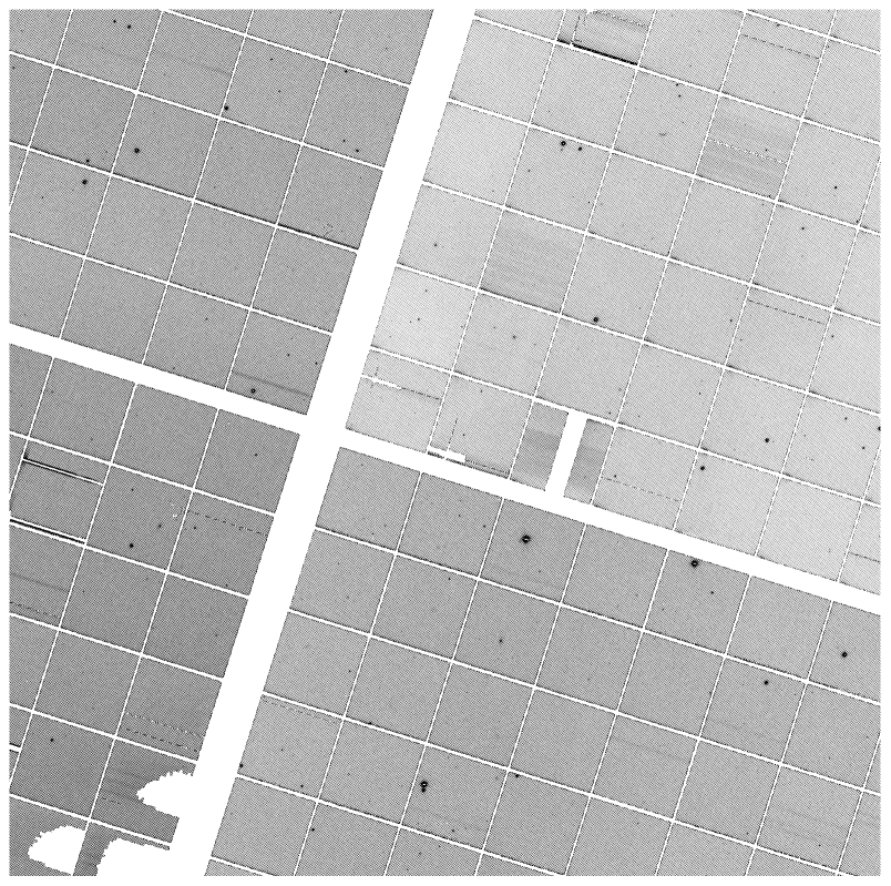
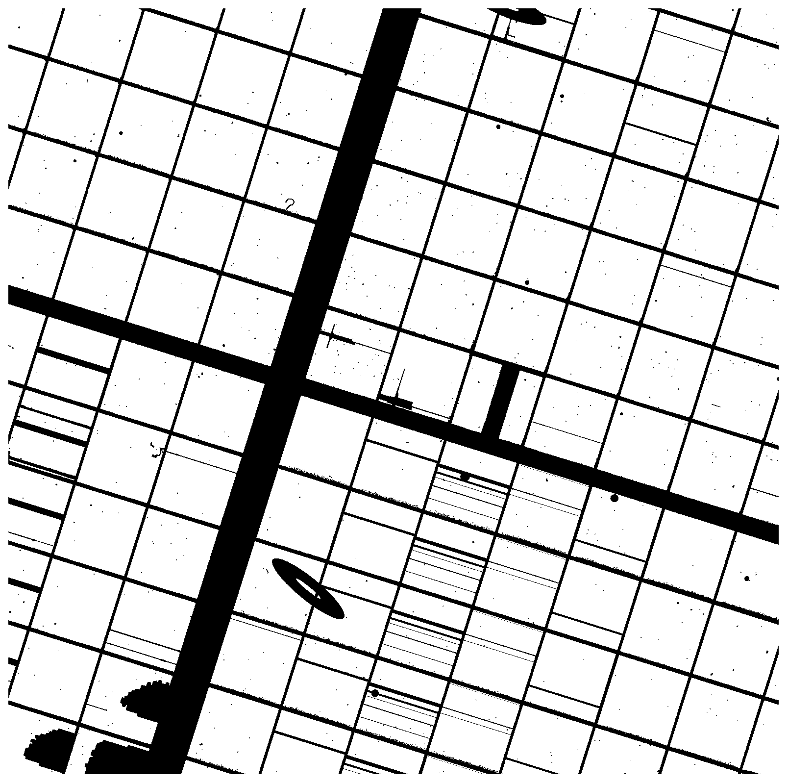
Figure 5 shows an example of the static mask for the full GPC1 field of view. Table 1 lists the bit mask values used for the different sources of masking.

Figure 5.— Image map of the GPC1 static mask. The CTE regions are clearly visible as roughly triangular patches covering the corners of some OTAs. Some entire cells are masked, including an entire column of cells on OTA14. Calcite cells remove large areas from OTA17 AND OTA76.

Table 1GPC1 Mask Values

Mask Name	Mask Value	Description (static values listed in bold)
DETECTOR	0x0001	A detector defect is present.
FLAT	0x0002	The flat field model does not calibrate the pixel reliably.
DARK	0x0004	The dark model does not calibrate the pixel reliably.
BLANK	0x0008	The pixel does not contain valid data.
CTE	0x0010	The pixel has poor charge transfer efficiency.
SAT	0x0020	The pixel is saturated.
LOW	0x0040	The pixel has a lower value than expected.
SUSPECT	0x0080	The pixel is suspected of being bad (overloaded with the BURNTOOL bit).
BURNTOOL	0x0080	The pixel contain an burntool repaired streak.
CR	0x0100	A cosmic ray is present.
SPIKE	0x0200	A diffraction spike is present.
GHOST	0x0400	An optical ghost is present.
STREAK	0x0800	A streak is present.
STARCORE	0x1000	A bright star core is present.
CONV.BAD	0x2000	The pixel is bad after convolution with a bad pixel.
CONV.POOR	0x4000	The pixel is poor after convolution with a bad pixel.
MARK	0x8000	An internal flag for temporarily marking a pixel.

3.6.2 Dynamic masks

In addition to the static mask that removes the constant detector defects, we also generate a set of dynamic masks that change with the astronomical features in the image. These masks are advisory in nature, and do not completely exclude the pixel from further processing consideration. The first of these dynamic masks is the burntool advisory mask described below. These pixels are included for photometry, but are rejected more readily in the stacking and difference image construction, as they are more likely to have small deviations due to imperfections in the burntool correction.

The remaining dynamic masks are generated in the IPP camera stage, at which point all object photometry is complete, and an astrometric solution is known for the exposure. This added information provides the positions of bright sources based on the reference catalog, including those that fall slightly out of the detector field of view or within the inter chip gaps, where internal photometry may not identify them. These bright sources are the origin for many of the image artifacts that the dynamic mask identifies and excludes.

Electronic crosstalk ghosts

Due to electrical crosstalk between the flex cables connecting the individual detector OTA devices, ghost objects can be created by the presence of a bright source at a different position on the camera. Table 2 summarizes the list of known crosstalk rules, with an estimate of the magnitude difference between the source and ghost. For all of the rules, any source cell $v$ within the specified column of cells on any of the OTAs in the specified column of OTAs $Y$ can create a ghost in the same cell $v$ and OTA $Y$ in the target column of cells and OTAs. This effect depends on the number of electrons detected for the star, thus the size of the ghost scales with the instrumental magnitude ($m_{inst}=-2.5\log_{10}(ADU)$) of the star. In each of these cases, a source object with $m_{inst}<-14.47$) (corresponding to $r_{\rm P1}\mathrel{\hbox{\hbox to0.0pt{\hbox{\lower 4.0pt\hbox{$\sim$}}\hss}\hbox{$<$}}}14$ for the $3\pi$ survey) creates a ghost object many orders of magnitude fainter at the target location. The cell ($x,y$) pixel coordinate is identical between source and ghost, as a result of the transfer occurring as the devices are read. A circular mask is added to the ghost location with radius $R=3.44\left(-14.47-m_{inst,source}\right)$ pixels; only positive radii are allowed. Any objects in the photometric catalog found at the location of the ghost mask have the GHOST mask bit set, marking the object as a likely ghost. The majority of the crosstalk rules are bi-directional, with a source in either position creating a ghost at the corresponding crosstalk target position. The two faintest rules are uni-directional, due to differences in the electronic path for the crosstalk.

For the very brightest sources ($m_{inst}<-15$), there can be crosstalk ghosts between all columns of cells during the readout. These “bleed” ghosts were originally identified as ghosts of the saturation bleeds appearing in the neighboring cells, and as such, the masking for these objects puts a rectangular mask down from top to bottom of cells in all columns that are in the same row of cells as the bright source. The width of this box is a function of the source magnitude, with $W=5\times\left(-15-m_{inst,source}\right)$ pixels.

Optical ghosts

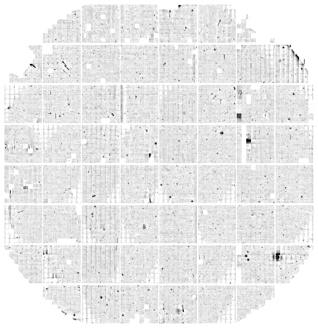
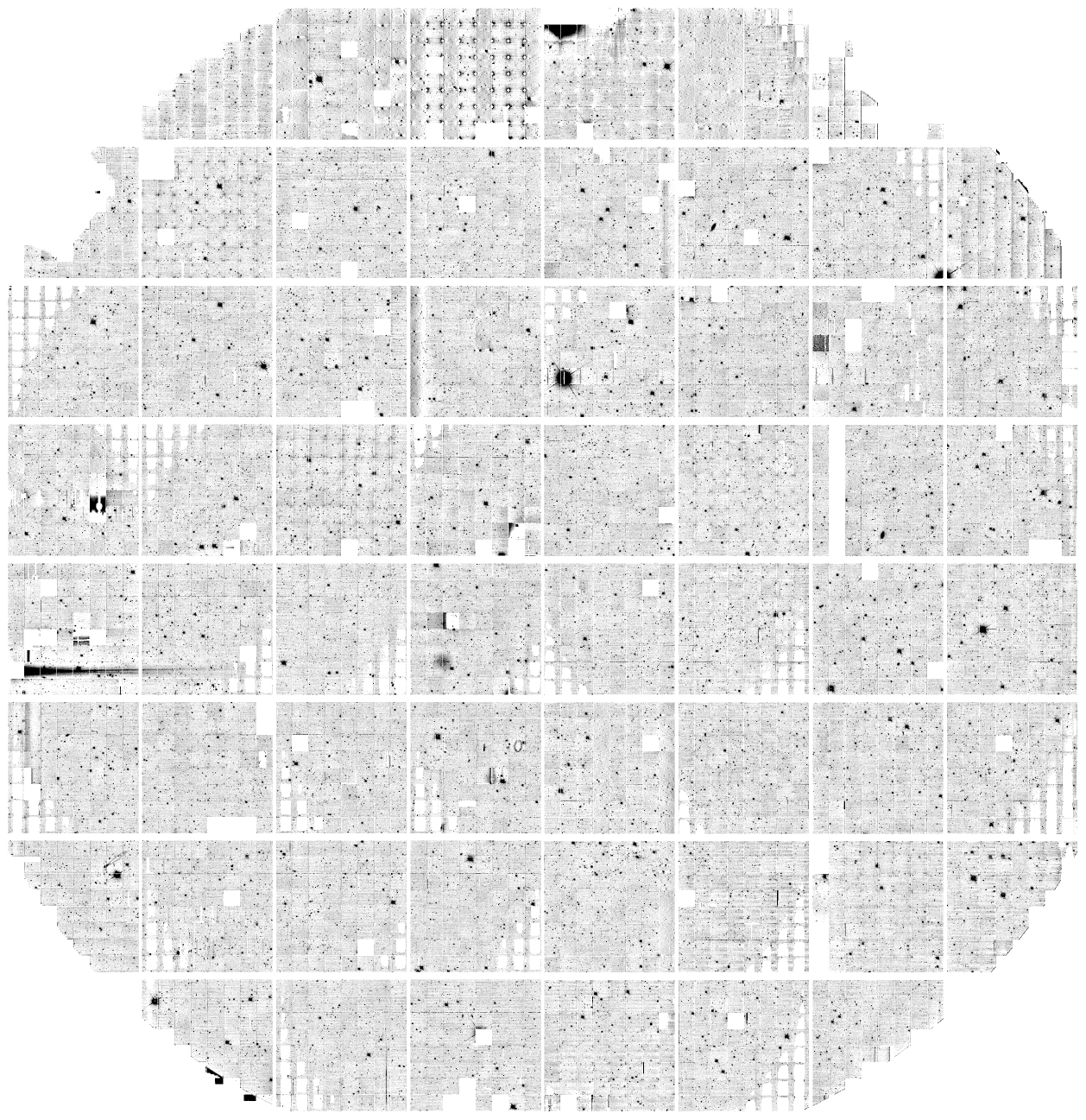
The anti-reflective coating on the optical surfaces of GPC1 is less effective at shorter wavelengths, which can allow bright sources to reflect back onto the focal plane and generate large out-of-focus objects. Due to the wavelength dependence, these objects are most prominent in the $g_{\rm P1}$ filter data. These objects are the result of light reflecting back off the surface of the detector, reflecting again off the lower surfaces of the optics (particularly the L1 corrector lens), and then back down onto the focal plane. Due to the extra travel distance, the resulting source is out of focus and elongated along the radial direction of the camera focal plane. Figure 6 shows an example exposure with several prominent optical ghosts.

These optical ghosts can be modeled in the focal plane coordinates ($L,M$) which has its origin at the center of the focal plane. In this system, a bright object at location ($L,M$) on the focal plane creates a reflection ghost on the opposite side of the optical axis near ($-L,-M$). The exact location is fit as a third order polynomial in the focal plane $L$ and $M$ directions (as listed in Table 3). An elliptical annulus mask is constructed at the expected ghost location, with the major and minor axes of the inner and outer elliptical annuli defined by linear functions of the ghost distance from the optical axis, and oriented with the ellipse major axis is along the radial direction (Table 4). All stars brighter than a filter-dependent threshold (listed in Table 5) have such masks constructed.

Table 2GPC1 Crosstalk Rules

Type	Source OTA/Cell	Ghost OTA/Cell	$\Delta m$
Inter-OTA	OTA2Y XY3v	OTA3Y XY3v	6.16
	OTA3Y XY3v	OTA2Y XY3v
	OTA4Y XY3v	OTA5Y XY3v
	OTA5Y XY3v	OTA4Y XY3v
Intra-OTA	OTA2Y XY5v	OTA2Y XY6v	7.07
	OTA2Y XY6v	OTA2Y XY5v
	OTA5Y XY5v	OTA5Y XY6v
	OTA5Y XY6v	OTA5Y XY5v
One-way	OTA2Y XY7v	OTA3Y XY2v	7.34
	OTA5Y XY7v	OTA4Y XY2v

Table 3Optical Ghost Center Transformations

Polynomial Term	$L$ center	$M$ center
$x^{0}y^{0}$	-1.215661e+02	2.422174e+01
$x^{1}y^{0}$	1.321875e-02	4.170486e-04
$x^{2}y^{0}$	-4.017026e-09	-1.934260e-08
$x^{3}y^{0}$	1.148288e-10	-1.173657e-12
$x^{0}y^{1}$	-1.908074e-03	1.189352e-02
$x^{1}y^{1}$	8.479150e-08	-9.256748e-08
$x^{2}y^{1}$	1.635732e-11	1.140772e-10
$x^{0}y^{2}$	2.625405e-08	8.123932e-08
$x^{1}y^{2}$	1.125586e-10	1.328378e-11
$x^{0}y^{3}$	2.912432e-12	1.170865e-10

Table 4Optical Ghost Annulus Axis Length

Radial Order	Inner Major Axis	Inner Minor Axis	Outer Major Axis	Outer Minor Axis
$r^{0}$	3.926693e+01	5.287548e+01	7.928722e+01	1.314265e+02
$r^{1}$	5.325759e-03	-2.191669e-03	1.722181e-02	-2.627153e-03

Table 5Optical Ghost Magnitude Limits

Filter	$m_{inst}$	Apparent mag ($3\pi$)
$g_{\rm P1}$	-16.5	12.2
$r_{\rm P1}$	-20.0	8.9
$i_{\rm P1}$	-25.0	3.7
$z_{\rm P1}$	-25.0	3.4
$y_{\rm P1}$	-25.0	2.5
$w_{\rm P1}$	-20.0	10.2

Optical glints

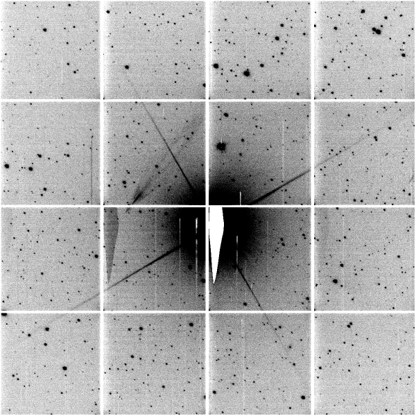
Prior to 2010-08-24, a reflective surface at the edge of the camera aperture was incompletely screened to light passing through the telescope. Sources brighter than $m_{inst}=-21$ ($r_{\rm P1}\mathrel{\hbox{\hbox to0.0pt{\hbox{\lower 4.0pt\hbox{$\sim$}}\hss}\hbox{$<$}}}7.5$) that fell on this reflective surface resulted in light being scattered across the detector surface in a long narrow glint. Figure 7 shows an example exposure with a prominent optical glint.

This reflective surface in the camera was physically masked on 2010-08-24, removing the possibility of glints in subsequent data, but images that were taken prior to this date have an advisory dynamic mask constructed when a reference source falls on the focal plane within one degree of the detector edge. This mask is 150 pixels wide, with length $L=2500\left(-20-m_{inst}\right)$ pixels. These glint masks are constructed by selecting sufficiently bright sources in the reference catalog that fall within rectangular regions around each edge of the GPC1 camera. These regions are separated from the edge of the camera by 17 arcminutes, and extend outwards an additional degree.

Diffraction Spikes and Saturated Stars

Bright sources also form diffraction spikes that are dynamically masked. These are filter independent, and are modeled as rectangles with length $L=10^{0.096\times(7.35-m_{inst})}-200$ and width $W=8+(L-200)\times 0.01$, with negative values indicating no mask is constructed, as the source is likely too faint to produce the feature. These spikes are dependent on the camera rotation, and are oriented based on the header keyword at $\theta=n\times\frac{\pi}{2}-\mathrm{ROTANGLE}+0.798$, for $n={0,1,2,3}$.

The cores of stars that are saturated are masked as well, with a circular mask radius $r=10.15\times(-15-m_{inst})$. An example of a saturated star, with the masked regions for the diffraction spikes and core saturation highlighted, is shown in Figure 8.

Saturation for the GPC1 detectors varies from chip to chip and cell to cell. Saturation levels have been measured in the lab for each cell and are recorded in the headers. The IPP analysis code reads the header value to determine the appropriate saturation point. Of the 3840 cells in GPC1, the median saturation level is 60,400; 95% have saturation levels $>54,500$ DN; 99% have saturation levels $>41,000$ DN. A small number of cells have recorded saturation values much lower than these values, but these also tend to be the cells for which other cosmetic effects (e.g., CTE & dark current) are strong, likely affecting the measurement of the saturation value.

Figure 6.— Ghosts: Example of the full GPC1 field of view illustrating the sources and destinations of optical ghosts on exposure o5677g0123o (2011-04-26, 43s $g_{\rm P1}$ filter). The bright stars on OTA33 and OTA44 result in nearly circular ghosts on the opposite OTA. In contrast, the trio of stars on OTA11 result in very elongated ghosts on OTA66.

Figure 7.— Glints: Example of a glint on exposure o5379g0103o (2010-07-02, 45s $i_{\rm P1}$ filter). The source star out of the field of view creates a long reflection that extends through OTA73 and OTA63.

Figure 8.— Example of saturated star, with diffraction spikes extending from the core on exposure o6802g0338o, OTA51 (2014-05-25, 45s $g_{\rm P1}$ filter).

3.6.3 Masking Fraction

The GPC1 camera was designed such that where possible, OTAs with CTE issues were placed towards the edge of the detector. Because of this, the main analysis of the mask fraction is based not on the total footprint of the detector, but upon a circular reference field of view with a radius of 1.5 degrees. This radius corresponds approximately to half the width and height of the detector. This field of view underestimates the unvignetted region of GPC1. A second “maximum” field of view is also used to estimate the mask fraction within a larger 1.628 degree radius. This larger radius includes far larger missing fractions due to the circular regions outside region populated with OTAs, but does include the contribution from well-illuminated pixels that are ignored by the reference radius.

The results of simulating the footprint of the detector as a grid of uniformly sized pixels of $0\hbox{$.\!\!^{\prime\prime}$}{}258$ size are provided in Table 6. Both fields of view contain circular segments outside of the footprint of the detector, which increase the area estimate that is unpopulated. This category also accounts for the inter-OTA and inter-cell gaps. The regions with poor CTE also contribute to a significant fraction of the masked pixels. The remaining mask category accounts for known bad columns, cells that do not calibrate well, and vignetting. There are also a small fraction that have static advisory masks marked on all images. These masks mark regions where bright columns on one cell periodically create cross talk ghosts on other cells.

During the camera processing, a separate estimate of the mask fraction for a given exposure is calculated by counting the fraction of pixels with static, dynamic, and advisory mask bits set within the two field of view radii. The static mask fraction is then augmented by an estimate of the unpopulated inter-chip gaps (as the input masks already account for the inter-cell gaps). This estimate does not include the circular segments outside of the detector footprint. This difference is minor for the reference field of view (1% difference), but underestimates the static mask fraction for the maximum radius by 7.3%. This analysis provides the observed dynamic and advisory mask fractions, which are 0.03% and 3% respectively. The significant advisory value is a result of applying such masks to all burntool corrected pixels.

Table 6Mask Fraction by Mask Source

Mask Source	3 Degree FOV	3.25 Degree FOV
Good pixel	78.9%	71.1%
Unpopulated	13.1%	19.6%
CTE issue	2.3%	2.6%
Other issue	5.4%	6.4%
Static advisory	0.3%	0.3%

3.7. Background subtraction

Once all other detrending is done, the pixels from each cell are mosaicked into the full $4846\times{}4868$ pixel OTA image. A background model for the full OTA is then determined prior to the photometric analysis. The mosaicked image is subdivided into $800\times{}800$ pixel segments that define each superpixel of the background model, with the superpixels centered on the image center and overlapping adjacent superpixels by 400 pixels. These overlaps help smooth the background model, as adjacent model pixels share input pixels.

From each segment, 10000 random unmasked pixels are drawn. In the case where the mask fraction is large (such as on OTAs near the edge of the field of view), and there are insufficient unmasked pixels to meet this criterion, all possible unmasked pixels are used instead. If this number is still small (less than 100 good pixels), the superpixel does not have a background model calculated. Instead, the value assigned to that model pixel is set as the average of the adjacent model pixels. This allows up to eight neighboring background values to be used to patch these bad pixels.

For the subdivisions that have sufficient unmasked pixels for the background to be measured, the pixel values are used to calculate a set of robust statistics for the initial background guess. The minimum and maximum of the values are found, and checked to ensure that these are not the same value, which would indicate some problem with the input values. The values are then inserted into a histogram with 1000 bins between the minimum and maximum values. If the bin with the most input pixels contains more than half of the input values, the bin size is too coarse for the population of interest. In this case, a new histogram is constructed using a range corresponding to the 20 bins closes to the peak, again dividing the range into 1000 bins. This process is iterated up to 20 times until a binsize is determined. A cumulative distribution is then constructed from the histogram, which saves the computational cost of sorting all the input values. The bins containing the 50-percentile point, as well as the 15.8%, 84.1% ($\pm 1\sigma$), 30.8%, 69.1% ($\pm 0.5\sigma$), 2.2%, and 97.7% ($\pm 2\sigma$) points are identified in this cumulative histogram. These bins, and the two bins to either side are then linearly interpolated to identify the pixel value corresponding to these points in the distribution. The 50% point is set as the median of the pixel distribution, with the standard deviation of the distribution set as the median of the $\sigma$ values calculated from the $0.5\times(\sigma_{+1}-\sigma_{-1})$, $\sigma_{+0.5}-\sigma_{-0.5}$, and $0.25\times(\sigma_{+2}-\sigma_{-2})$ differences. If this measured standard deviation is smaller than 3 times the bin size, then all points more than 25 bins away from the calculated median are masked, and the process is repeated with a new 1000 bin histogram until the bin size is sufficiently small to ensure that the distribution width is well sampled. Once this iterative process converges, or 20 iterations are run, the 25- and 75-percentile values are found by interpolating the 5 bins around the expected bin as well, and the count of the number of input values within this inner 50-percentile region, $N_{50}$, is calculated.

These initial statistics are then used as the starting guesses for a second calculation of the background level that attempts to fit the distribution with a Gaussian. All pixels that were masked in the initial calculation are unmasked, and a histogram is again constructed from the values, with a bin size set to $\sigma_{guess}/\left(N_{50}/500\right)$. With this bin size, we expect that a bin at $\pm 2\sigma$ will have approximately 50 input points, which gives a Poissonian signal-to-noise estimate around 7. In the case where $N_{50}$ is small (due to a poorly populated input image), this bin size is fixed to be no larger than the guess of the standard deviation. The endpoints of the histogram are clipped based on the input guesses, such that any input point with a value more than $5\sigma_{guess}$ away from the input mean are excluded from consideration.

Two second order polynomial fits are then performed to the logarithm of the histogram counts set at the midpoint of each bin. The first fit considers the lower portion of the distribution, under the assumption that deviations from a normal distribution are caused by real astrophysical sources that will be brighter than the true background level. From the bin with most pixel values, the lower bound is set by searching for the first bin from the peak that has fewer inputs than 25% of the peak. A similar search is performed for the upper bound, but with a criterion that the bin has fewer than 50% of the peak. On both sides of the peak, the bounds are adjusted to ensure that at least seven bins, equally distributed around the peak, are used. The second fit is symmetric, fitting both sides of the distribution out to the point where the bin contains fewer than 15% of the peak value. The same seven-bin constraint is used for this fit. The Gaussian mean and standard deviation are calculated from the polynomial coefficients, and the symmetric fit results are accepted unless the lower-half fit results in a smaller mean. This histogram and polynomial fit process is repeated again, with updated bin size based on the previous iteration standard deviation, if the calculated standard deviation is not larger than 75% of the initial guess (suggesting an issue with the initial bin size).

With this two-stage calculation performed across all subdivisions of the mosaicked OTA image, and missing model pixels filled with the average of their neighbors, the final background model is stored on disk as a $13\times{}13$ image for the GPC1 chips with header entries listing the binning used. The full scale background image is then constructed by bilinearly interpolating this binned model, and this is subtracted from the science image. Each object in the photometric catalog has a SKY and SKY_SIGMA value determined from the background model mean and standard deviation.

Although this background modeling process works well for most of the sky, astronomical sources that are large compared to the $800\times{}800$ pixel subdivisions can bias the calculated background level high, resulting in an oversubtraction near that object. The most common source that can cause this issue are large galaxies, which can have their own features modeled as being part of the background. For the specialized processing of M31, which covers an entire pointing of GPC1, the measured background was added back to the chip stage images, but this special processing was not used for the large scale $3\pi$ PV3 reduction.

3.8. Burntool / Persistence effect

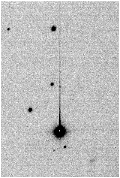
Pixels that approach the saturation point on GPC1 (see Section 3.6.2) introduce “persistent charge” on that and subsequent images. During the read out process of a cell with such a bright pixel, some of the charge remains in the undepleted region of the silicon and is not shifted down the detector column toward the amplifier. This charge remains in the starting pixel and slowly leaks out of the undepleted region, contaminating subsequent pixels during the read out process, resulting in a “burn trail” that extends from the center of the bright source away from the amplifier (vertically along the pixel columns toward the top of the cell).

This incomplete charge shifting in nearly full wells continues as each row is read out. This results in a remnant charge being deposited in the pixels that the full well was shifted through. In following exposures, this remnant charge leaks out, resulting in a trail that extends from the initial location of the bright source on the previous image towards the amplifier (vertically down along the pixel column). This remnant charge can remain on the detector for up to thirty minutes.

Both of these types of persistence trails are measured and optionally repaired via the burntool program. This program does an initial scan of the image, and identifies objects with pixel values higher than a conservative threshold of 30000 DN. The trail from the peak of that object is fit with a one-dimensional power law in each pixel column above the threshold, based on empirical evidence that this is the functional form of this persistence effect. This fit also matches the expectation that a constant fraction of charge is incompletely transferred at each shift beyond the persistence threshold. Once the fit is done, the model can be subtracted from the image. The location of the source is stored in a table along with the exposure PONTIME, which denotes the number of seconds since the detector was last powered on and provides an internally consistent time scale.

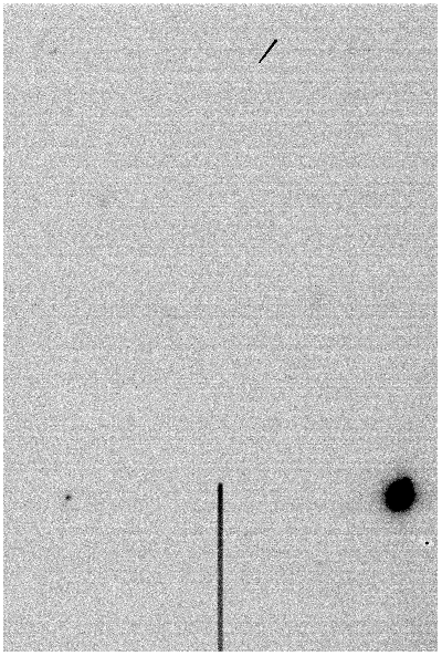
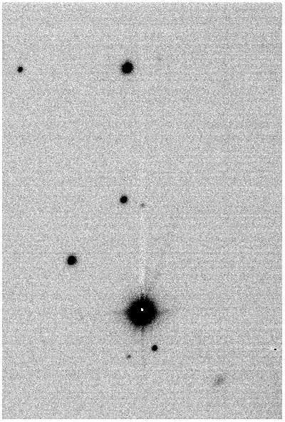
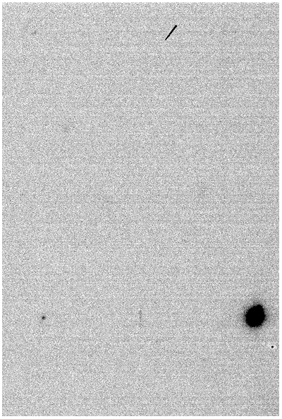
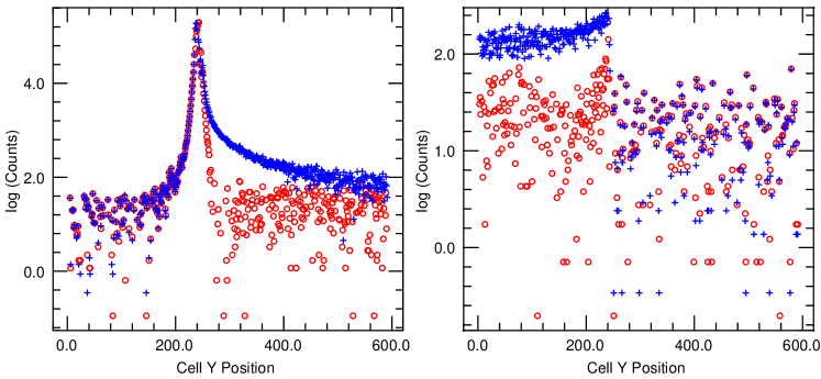
For subsequent exposures, the table associated with the previous image is read in, and after correcting trails from the stars on the new image, the positions of the bright stars from the table are used to check for remnant trails from previous exposures on the image. These are fit and subtracted using a one-dimensional exponential model, again based on empirical studies. The output table retains this remnant position for 2000 seconds after the initial PONTIME recorded. This allows fits to be attempted well beyond the nominal lifetime of these trails. Figure 9 shows an example of a cell with a persistence trail from a bright star, the post-correction result, as well as the pre and post correction versions of the same cell on the subsequent exposure. The profiles along the detector columns for these two exposures are presented in Figure 10.

Using this method of correcting the persistence trails has the challenge that it is based on fits to the raw image data, which may have other signal sources not determined by the persistence effect. The presence of other stars or artifacts in the detector column can result in a poor model to be fit, resulting in either an over- or under-subtraction of the trail. For this reason, the image mask is marked with a value indicating that this correction has been applied. These pixels are not fully excluded, but they are marked as suspect, which allows them to be excluded from consideration in subsequent stages, such as image stacking.

The cores of very bright stars can also be deformed by this process, as the burntool fitting subtracts flux from only one side of the star. As most stars that result in persistence trails already have saturated cores, they are already ignored for the purpose of PSF determination and are flagged as saturated by the photometry reduction.

Figure 9.— Persistent Charge: Example of OTA11 cell xy50 on exposures o5677g0123o (left) and o5677g0124o (right). The top panels show the image with all appropriate detrending steps, but without burntool, and the bottom show the same with burntool applied. There is some slight over subtraction in fitting the initial trail, but the impact of the trail is greatly reduced in both exposures.

Figure 10.— Burntool Correction: Example of a profile cut along the y-axis through a bright star on exposure o5677g0123o OTA11 in cell xy50 (left panel) and on the subsequent exposure o5677g0124o (right panel). In both figures, the blue pluses show the image corrected with all appropriate detrending steps, but without burntool applied, illustrating the amplitude of the persistence trails. The red circles show the same data after the burntool correction, which reduces the impact of these features. Both exposures are in the $g_{\rm P1}$ filter with exposure times of 43s

3.9. Non-linearity Correction

The pixels of GPC1 are not uniformly linear at all flux levels. In particular, at low flux levels, some pixels have a tendency to sag relative to the expected linear value. This effect is most pronounced along the edges of the detector cells, although some entire cells show evidence of this effect.

To correct this sag, we studied the behavior of a series of flat frames for a ramp of exposure times with approximate logarithmically equal spacing between 0.01s and 57.04s. As the exposure time increases, the signal on each pixel also increases in what is expected to be a linear manner. Each of the flat exposures in this ramp is overscan corrected, and then the median is calculated for each cell, as well as for the rows and columns within ten pixels of the edge of the science region. From these median values at each exposure time value, we can construct the expected trend by fitting a linear model for the region considered. This fitting was limited to only the range of fluxes between 12000 and 38000 counts, as these ranges were found to match the linear model well. This range avoids the non-linearity at low fluxes, as well as the possibility of high-flux non-linearity effects.

We store the average flux measurement and deviation from the linear fit for each exposure time for each region on all detector cells in the linearity detrend look-up tables. When this correction is applied to science data, these lookup tables are loaded, and a linear interpolation is performed to determine the correction needed for the flux in that pixel. This look up is performed for both the row and column of each pixel, to allow the edge correction to be applied where applicable, and the full cell correction elsewhere. The average of these two values is then applied to the pixel value, reducing the effects of pixel nonlinearity.

This non-linearity effect appears to be stable in time for the majority of the detector pixels, with little evident change over the survey duration. However, as the non-linearity is most pronounced at the edges of the detector cells, those are the regions where the correction is most likely to be incomplete. Because of this fact, most pixels in the static mask with either the DARKMASK or FLATMASK bit set are found along these edges. As the non-linearity correction is unable to reliably restore these pixels, they produce inconsistent values after the dark and flat have been applied, and are therefore rejected.

3.10. Pattern correction

3.10.1 Pattern Row

As discussed above in the dark and noisemap sections, certain detectors have significant bias offsets between adjacent rows, caused by drifts in the bias level due to cross talk. The magnitude of these offsets increases as the distance from the readout amplifier and overscan region increases, resulting in horizontal streaks that are more pronounced along the large $x$ pixel edge of the cell. As the level of the offset is apparently random between exposures, the dark correction cannot fully remove this structure from the images, and the noisemap value only indicates the level of the average variance added by these bias offsets. Therefore, we apply the PATTERN.ROW correction in an attempt to mitigate the offsets and correct the image values. To force the rows to agree, a second order clipped polynomial is fitted to each row in the cell. Four fit iterations are run and pixels $2.5\sigma$ deviant (chosen empirically) are excluded from subsequent fits in order to minimize the bias from stars and other astronomical sources in the pixels. This final trend is then subtracted from that row. Simply doing this subtraction will also have the effect of removing the background sky level. To prevent this, the constant and linear terms for each row are stored, and linear fits are made to these parameters as a function of row, perpendicular to the initial fits. This produces a plane that is added back to the image to restore the background offset and any linear ramp that exists in the sky.

These row-by-row variations have the largest impact on data taken in the $g_{\rm P1}$ filter, as the read noise is the dominant noise source in that filter. At longer wavelengths, the noise from the Poissonian variation in the sky level increases. The PATTERN.ROW correction is still applied to data taken in the other filters, as the increase in sky noise does not fully obscure the row-by-row noise.

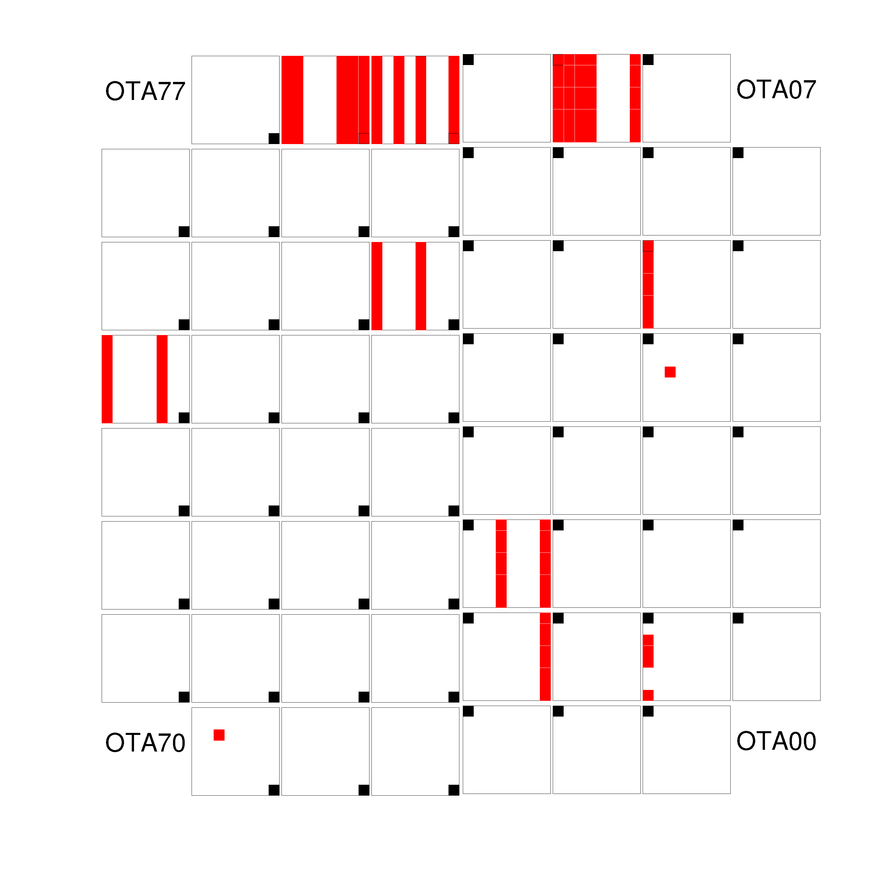
This correction was required on all cells on all OTAs prior to 2009-12-01, at which point a modification of the camera clocking phase delays reduced the scale of the row-by-row offsets for the majority of the OTAs. As a result, we only apply this correction to the cells where it is still necessary, as shown in Figure 11. A list of these cells is in Table 7.

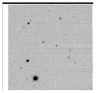
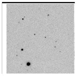
Although this correction largely resolves the row-by-row offset issue in a satisfactory way, large and bright astronomical objects can bias the fit significantly. This results in an oversubtraction of the offset near these objects. As the offsets are calculated on the pixel rows, this oversubtraction is not uniform around the object, but is preferentially along the horizontal x axis of the object. Most astronomical objects are not significantly distorted by this, with this only becoming on issue for only bright objects comparable to the size of the cell (598 pixels = 150"). Figure 12 shows an example of a cell pre- and post-correction.

Table 7Cells which have PATTERN.ROW correction applied

OTA	Cell columns	Additional cells
OTA11		xy02, xy03, xy04, xy07
OTA14		xy23
OTA15	0
OTA27	0, 1, 2, 3, 7
OTA31	7
OTA32	3, 7
OTA45	3, 7
OTA47	0, 3, 5, 7
OTA57	0, 1, 2, 6, 7
OTA60		xy55
OTA74	2, 7

Figure 11.— Diagram illustrating in red which cells on GPC1 require the PATTERN.ROW correction to be applied. The footprint of each OTA is outlined, and cell xy00 is marked with either a filled box or an outline. The labeling of the non-existent corner OTAs is provided to orient the focal plane.

Figure 12.— Correlated Noise: Example of the PATTERN.ROW correction on exposure o5379g0103o OTA57 cell xy01 ($i_{\rm P1}$ filter 45s). The left panel shows the cell with all appropriate detrending except the PATTERN.ROW, and the right shows the same cell with PATTERN.ROW applied. The correction reduces the correlated noise on the right side, which is most distant from the read out amplifier. There is a slight over subtraction along the rows near the bright star.

3.10.2 Pattern Continuity

The background sky levels of cells on a single OTA do not always have the same value. Despite having dark and flat corrections applied, adjacent cells may not match even for images of nominally empty sky. In addition, studies of the background level indicate that the row-by-row bias can introduce small background gradient variations along the rows of the cells that are not stable. This common feature across the columns of cells results in a “saw tooth” pattern horizontally across an the mosaicked OTA, and as the background model fits a smooth sky level, this induces over- and under subtraction at the cell boundaries.

The PATTERN.CONTINUITY correction, attempts to match the edges of a cell to those of its neighbors. For each cell, a thin box 10 pixels wide running the full length of each edge is extracted and the median of unmasked values is calculated for that box. These median values are then used to construct a vector of the sum of the differences between that cell’s edges and the corresponding edge on any adjacent cell $\Delta$. A matrix $A$ of these associations is also constructed, with the diagonal containing the number of cells adjacent to that cell, and the off-diagonal values being set to -1 for each pair of adjacent cells. The offsets needed for each chip, $\zeta$ can then be found by solving the system $A\zeta=\Delta$. A cell with the maximum number of neighbors, usually cell xy11, the first cell not on the edge of the OTA, is used to constrain the system, ensuring that that cell has zero correction and that there is a single solution.

For OTAs that initially show the saw tooth pattern, the effect of this correction is to align the cells into a single ramp, at the expense of the absolute background level. However, as we subtract off a smooth background model prior to doing photometry, these deviations from an absolute sky level do not affect photometry for point sources and extended sources smaller than a single cell. The fact that the final ramp is smoother than it would be otherwise also allows for the background subtracted image to more closely match the astronomical sky, without significant errors at cell boundaries. An example of the effect of this correction on an image profile is shown in Figure 2.

4. GPC1 Detrend Construction

The various master detrend images for GPC1 are constructed using a common approach. A series of appropriate exposures is selected from the database, and processed with the ppImage program, which is designed to do multiple image processing operations. The processing steps applied to the images depend on the type of master detrend to be constructed. In general, the input exposures to the detrend have all prior stages of detrend processing applied. Table 8 summarizes stages applied for the detrends we construct.

Once the input data has been prepared, the ppMerge program is used to combine the inputs. In some cases, this is the mathematical average, but in other cases it is a fit across the inputs. Table 9 lists some of the properties of the process for the detrends, including how discrepant values are removed and the combination method used. The outputs from this step have the format of the detrend under construction. After construction, these combined outputs are applied to the processed input data. This creates a set of residual files that are checked to determine if the newly created detrend correctly removes the detector dependent signal.

This process of detrend construction and testing can be iterated, with individual exposures excluded if they are found to be contaminating the output. The construction of detrends is largely automatic, but manual intervention is needed to accept the detrend for use on science data. If the final detrend has sufficiently small residuals, then the iterations are stopped and the detrend is finalized by selecting the date range to which it applies. This allows subsequent science processing to select the detrends needed based on the observation date. Table 10 lists the set of detrends used in the PV3 processing.

Table 8Detrend Construction Processing

Detrend Type	Overscan Subtracted	Nonlinearity Correction	Dark Subtracted	Flat Applied
LINEARITY	Y
DARK	Y	Y
FLAT	Y	Y	Y
FRINGE	Y	Y	Y	Y
DARKMASK	Y	Y	Y
FLATMASK	Y	Y	Y	Y
CTEMASK	Y	Y	Y	Y
NOISEMAP	Y	Y

Table 9Detrend Merge Options

Detrend Type	Iterations	Threshold	Additional Clipping	Combination Method
DARKMASK	3	$8\sigma$		Mask if $>10\%$ rejected
FLATMASK	3	$3\sigma$		Mask if $>10\%$ rejected
CTEMASK	2	$2\sigma$		Clipped mean; mask if $\sigma^{2}/\langle I\rangle<0.5$
DARK	2	$3\sigma$		Clipped mean
NOISEMAP	2	$3\sigma$		Mean
FLAT	1	$3\sigma$	Top $30\%$; Bottom $10\%$	Mean
FRINGE	2	$3\sigma$		Clipped mean

Table 10PV3 Detrends

Detrend Type	Detrend ID	Start Date (UT)	End Date (UT)	Note
LINEARITY	421	2009-01-01 00:00:00
MASK	945	2009-01-01 00:00:00
	946	2009-12-09 00:00:00
	947	2010-01-01 00:00:00
	948	2011-01-06 00:00:00
	949	2011-03-09 00:00:00	2011-03-10 23:59:59
	950	2011-08-02 00:00:00
	1072	2015-12-17 00:00:00		Update OTA62 mask
DARK	223	2009-01-01 00:00:00	2009-12-09 00:00:00
	229	2009-12-09 00:00:00
	863	2010-01-23 00:00:00	2011-05-01 00:00:00	A-mode
	864	2011-05-01 00:00:00	2011-08-01 00:00:00
	865	2011-08-01 00:00:00	2011-11-01 00:00:00
	866	2011-11-01 00:00:00	2019-04-01 00:00:00
	869-935	2010-01-25 00:00:00	2011-04-25 23:59:59	B-mode
VIDEODARK	976	2009-01-01 00:00:00	2009-12-09 00:00:00
	977	2009-12-09 00:00:00	2010-01-23 00:00:00
	978	2010-01-23 00:00:00	2011-05-01 00:00:00	A-mode
	979	2011-05-01 00:00:00	2011-08-01 00:00:00
	980	2011-08-01 00:00:00	2011-11-01 00:00:00
	981	2011-11-01 00:00:00	2019-04-01 00:00:00
	982-1048	2010-01-25 00:00:00	2011-04-25 23:59:59	B-mode
	1049	2010-09-12 00:00:00	2011-05-01 00:00:00	A-mode with OTA47fix
NOISEMAP	963	2008-01-01 00:00:00	2010-09-01 00:00:00
	964	2010-09-01 00:00:00	2011-05-01 00:00:00
	965	2011-05-01 00:00:00
FLAT	300	2009-12-09 00:00:00		$g_{\rm P1}$ filter
	301	2009-12-09 00:00:00		$r_{\rm P1}$ filter
	302	2009-12-09 00:00:00		$i_{\rm P1}$ filter
	303	2009-12-09 00:00:00		$z_{\rm P1}$ filter
	304	2009-12-09 00:00:00		$y_{\rm P1}$ filter
	305	2009-12-09 00:00:00		$w_{\rm P1}$ filter
FRINGE	296	2009-12-09 00:00:00
ASTROM	1064	2008-05-06 00:00:00

5. Warping

In order to perform image combination operations (stacking and differences), the individual OTA images are geometrically transformed to a set of images with a consistent and uniform relationship between sky coordinates and image pixels. This warping operation transforms the image pixels from the regular grid laid out on the chips in the camera to a system of pixels with consistent geometry for a location on the sky.

The new image coordinate system is defined by one of a number of “tessellations” which specify how the sky is divided into individual images. A single tessellation starts with a collection of projection centers distributed across the sky. A grid of image pixels about each projection center corresponds to sky positions via a projection with a specified pixel scale and rotation. In general, the pixel grid within the projection is defined as a simplified grid with the y-axis aligned to the Declination lines and no distortion terms. The projection centers are typically separated by several degrees on the sky; for pixel scales appropriate to GPC1, the resulting collection of pixels would be unwieldy in terms of memory in the processing computer. The pixel grid is thus subdivided into smaller sub-images called ’skycells’.

A tessellation can be defined for a limited region, with only a small number of projection centers (e.g., for processing the M31 region), or even a single projection center (e.g., for the Medium Deep fields). For the $3\pi$ survey, the tessellation contains projection centers covering the entire sky. The version used to for the PV3 analysis is called the RINGS.V3. This tessellation consists of 2643 projection centers spaced every four degrees in DEC, with RA spacing of approximately four degrees, adjusted to ensure an integer number of equal-sized regions. RINGS.V3 uses a pixel scale of $0\hbox{$.\!\!^{\prime\prime}$}{}25$ per pixel. The projections subdivided into a $10\times{}10$ grid of skycells, with an overlap region of 60^′′ between adjacent skycells to ensure that objects of modest size are not split on all images. The coordinate system used for these images matches the parity of the sky, with north in the positive $y$ direction and east to the negative $x$ direction.

After the detrending and photometry, the detection catalog for the full camera is fit to the reference catalog, producing astrometric solutions that map the detector focal plane to the sky, and map the individual OTA pixels to the detector focal plane (see Magnier et al., 2016a). This solution is then used to determine which skycells the exposure OTAs overlap.

For each output skycell, all overlapping OTAs and the calibrated catalog are read into the pswarp program. The output warp image is broken into $128\times{}128$ pixel grid boxes. For purposes of speed, each grid box has a locally linear map calculated that converts the output warp image coordinates to the input chip image coordinates. By doing the transformation in this direction, each output pixel has a unique sampling position on the input image (although it may be off the image frame and therefore not populated), guaranteing that all output pixels are addressed, and thus preventing gaps in the output image due to the spacing of the input pixels.

With the locally linear grid defined, Lanczos interpolation (Lanczos, 1956) with filter size parameter $a=3$ on the input image is used to determine the values to assign to the output pixel location. This interpolation kernel was chosen as a compromise between simple interpolations and higher-order Lanczos kernels, with the goal of limiting the smear in the output image while avoiding the high-frequency ringing generated by higher order kernels. This process is repeated for all grid boxes, for all input images, and for each output image product: the science image, the variance, and the mask. The image values are scaled by the absolute value of the Jacobian determinant of the transformation for each grid box. This corrects the pixel values for the possible change in pixel area due to the transformation. Similarly, the variance image is scaled by the square of this value, again to correctly account for the pixel area change.

The interpolation constructs the output pixels from more than one input pixel, which introduces covariance between pixels. For each locally-linear grid box, the covariance matrix is calculated from the kernel in the center of the 128 pixel range. Once the image has been fully populated, this set of individual covariance matrices are averaged to create the final covariance for the full image.

An output catalog is also constructed from the full exposure input catalog, including only those objects that fall on the new warped image. These detections are transformed to match the new image location, and to scale the position uncertainties based on the new orientation.

The output image also contains header keywords SRC_nnnn, SEC_nnnn, MPX_nnnn, and MPY_nnnn that define the mappings from the warped pixel space to the input images. The ’nnnn’ for each keyword has the values 0000, 0001, etc., up to the number of input images. The SRC keyword lists the input OTA name, and the SEC keyword lists the image section that the mapping covers. The MPX and MPY contain the back-transformation linearized across the full chip. These parameters are stored in a string listing the reference position in the chip coordinate frame, the slope of the relation in the warp $x$ axis, and the slope of the relation in the warp $y$ axis. From these keywords, any position in the warp can be mapped back to the location in any of the input OTA images, with some reduction in accuracy.

Examples of a warped signal, variance, and mask image are illustrated in Figures 13 through 15.

Figure 13.— Example of the warp image for skycell skycell.1146.095 centered at ($\alpha,\delta$) = (11.934, -4.197) for exposure o5104g0266o, (2009-09-30, 60s $r_{\rm P1}$ filter). The data from four OTAs contribute to this image, although they are all truncated by the skycell boundaries. This skycell image is aligned such that north points to the top of the image, and east to the left. The contributing OTAs are OTA20, OTA21, OTA30, OTA31.

Figure 14.— Example of the warp variance image for skycell skycell.1146.095 of exposure o5104g0266o, the same as in Figure 13. This variance map retains information about the higher flux levels that were found in burntool corrected persistence trails, which appear here as streaks along the original OTA y axis. The dark glows that are corrected in the dark model are also more visible, especially on certain cell edges. As both of these effects are corrected in the science image, there are no significant features visible there.

Figure 15.— Example of the warp mask image for skycell skycell.1146.095 of exposure o5104g0266o, the same as in Figure 13. This mask image shows the many small defects removed from the image, along with larger advisory trails on corrected burntool trails. The saturated cores of the bright stars are also masked, along with the diffraction spikes found on these stars. A ghost mask is visible just below the center as an elliptical region.

6. Stacking

Once individual exposures have been warped onto a common projection system, they can be combined pixel-by-pixel regardless of their original orientation. Creating a stacked image by co-adding the individual warps increases the signal to noise, allowing for the detection of objects that would not be sufficiently significant to be measured from a single image. Creating this stack also allows a more complete image to be constructed that has fewer regions masked due to the gaps between cells and OTAs. This deeper and more complete image can also be used as a template for subtraction to find transient sources.

As part of the stacking process, the collection of input pixels for a given output stack pixel are checked for consistency and outliers are rejected. Varying image quality makes a pixel-by-pixel check for outliers challenging in the vicinity of brighter stars. Pixels in the wings of bright stars are liable to be over-rejected as the image quality changes because the flux observed at a given position varies as its location on the stellar profile changes. To avoid this effect, we convolve all input images to a common PSF before making the pixel-by-pixel comparison. This PSF-matching technique allows us to detect inconsistent pixels even in the sensitive wings of bright objects.

For the $3\pi$ survey, the stacked image is comprised of all warp frames for a given skycell in a single filter. The source catalogs and image components are loaded into the ppStack program to prepare the inputs and stack the frames.

Once all files are ingested, the first step is to measure the size and shapes of the input image PSFs. We exclude images that have a PSF FWHM greater than 10 pixels (2.5 arcseconds), as those images have the seeing far worse than average, and would degrade the final output stack. For the PV3 processing of the $3\pi$ survey, this size represents a PSF larger than the $97$th percentile in all filters. A target PSF for the stack is constructed by finding the maximum envelope of all input PSFs, which sets the target PSF to the largest value among the input PSFs for a given position from the peak. This PSF is then circularized to ensure azimuthal symmetry, which prevents deconvolution of any of the input images when matched to the target.

The input image fluxes are normalized to prevent differences in seeing and sky transparency from causing discrepancies during pixel rejection. From the reference catalog calibrated input catalogs, we have the instrumental magnitudes of all sources, along with the airmass, image exposure time, and zeropoint. All output stacks are constructed to a target zeropoint of 25.0 in all filters, and to have an airmass of 1.0. The target zeropoint is arbitrary; 25.0 was chosen to be roughly consistent with the PS1 zero points, while still being a simple number. The output exposure time is set to the sum of the input exposure times, regardless of whether those inputs are rejected later in the combination process. We can determine the relative transparency for each input image by comparing the magnitudes of matched sources between the different images. Each image then has a normalization factor defined, equal to $\mathrm{norm}_{input}=(ZP_{\mathrm{input}}-ZP_{\mathrm{target}})-\mathrm{transparency}_{\mathrm{input}}-2.5\times\log_{10}(t_{\mathrm{target}}/t_{\mathrm{input}})-\mathrm{F}_{\mathrm{airmass}}\times(\mathrm{airmass}_{\mathrm{input}}-\mathrm{airmass}_{\mathrm{target}})$. For the PV3 processing, the airmass factor $\mathrm{F}_{\mathrm{airmass}}$ was set to zero, such that all flux differences from differing exposure airmasses are assumed to be included in the zeropoint and transparency values.

The zeropoint calibration performed here uses the calibration of the individual input exposures against the reference catalog. Upon the conclusion of the survey, the entire set of detection catalogs is further re-calibrated in the “ubercal” process (Schlafly et al., 2012). This produces a more consistent calibration of each exposure across the entire region of the sky imaged. This further calibration is not available at the time of stacking, and so there may be small residuals in the transparency values as a result of this (Magnier et al., 2016a).

With the flux normalization factors and target PSF chosen, the convolution kernels can be calculated for each image. To calculate the convolution kernels, we use the algorithm described by Alard & Lupton (1998) and extended by Alard (2000) to perform optimal image subtraction. These ‘ISIS’ kernels (named after the software package described by Alard & Lupton, 1998) are used with FWHM values of 1.5, 3.0, and 6.0 pixels and polynomial orders of 6, 4, and 2. Regions around the sources identified in the input images are extracted, convolved with the kernel, and the residual with the target PSF used to update the parameters of the kernel via least squares optimization. Stamps that significantly deviate are rejected, although the squared residual difference will increase with increasing source flux. To mitigate this effect, a parabola is fit to the distribution of squared residuals as a function of source flux. Stamps that deviate from this fit by more than $2.5\sigma$ are rejected, and not used on further kernel fit iterations. This process is repeated twice, and the final convolution kernel is returned.

This convolution may change the image flux scaling, so the kernel is normalized to account for this. The normalization factor is equal to the ratio of $10^{-0.4\mathrm{norm}_{input}}$ to the sum of the kernel. The image is multiplied by this factor, and the variance by the square of it, scaling all inputs to the common zeropoint.

Once the convolution kernels are defined for each image, they are used to convolve the image to match the target PSF. Any input image that has a kernel match $\chi^{2}$ value (defined as the sum of the RMS error across the kernel) 4.0$\sigma$ or larger than the median value is rejected from the stack. Each image also has a weight assigned, based on the image variance after convolution. A full image weight is then calculated for each input, with the weight, $W_{\mathrm{input}}$ equal to the inverse of the median of the image variance multiplied by the peak of the image covariance (from the warping process). This ensures that low signal-to-noise images are down-weighted in the final combination.

Following the convolution, an initial stack is constructed. For a given pixel coordinate, the values at that coordinate are extracted from all input images, with pixels masked excluded from consideration. Images that only have a suspect mask bit (including the SUSPECT, BURNTOOL, SPIKE, STREAK, STARCORE, and CONV.POOR bit values) are appended to a suspect pixel list for preferential exclusion. Following this, the pixel values are combined and tested to attempt to identify discrepant input values that should be excluded.

If only a single input is available, the initial stack contains the value from that single input. If there are only two inputs, the average of the two is used. These cases are expected to occur only rarely in the $3\pi$ survey, as there are many input exposures that overlap each point on the sky. For the more common case of three or more inputs, a weighted average from the inputs is used, with the weight for each image as defined above used for all pixels from that input image. This weight is used for both the image and the exposure weighted image:

$$\mathrm{Stack}_{\mathrm{value}} = \sum_{i}\left(\mathrm{value}_{\mathrm{input}}\times W_{\mathrm{input}}\right)/\sum_{\mathrm{inputs}}\left(W_{\mathrm{input}}\right)$$ (1)

$$\mathrm{Stack}_{\mathrm{expweight}} = \sum_{i}\left(\mathrm{exptime}_{\mathrm{input}}\times W_{\mathrm{input}}\right)/\sum_{\mathrm{inputs}}\left(W_{\mathrm{input}}\right)$$ (2)

The pixel exposure time is simply the sum of the input exposure time values, and the output variance is

$$\mathrm{Stack}_{\mathrm{variance}} = 1/\sum_{i}\left(1/\sigma^{2}_{\mathrm{input}}\right)$$ (4)

The output mask value is taken to be zero (no masked bits), unless there were no valid inputs, in which case the BLANK mask bit is set.

Due to uncorrected artifacts that can occur on GPC1, and the fact that they may not be fully masked to ensure all bad pixels are removed, it is expected that some of the inputs for a given stack pixel are not in agreement with the others. In general, there is the population of input pixel values around the correct astronomical level, as well as possible populations at lower pixel value (such as due to an over-subtracted burntool trail) and at higher pixel values (such as that caused by an incompletely masked optical ghost). Due to the observation strategy to observe a given field twice to allow for warp-warp difference images to be constructed to identify transient detections, higher pixel values that come from sources like optical ghosts that depend on the telescope pointing will come in pairs. Detector artifacts will appear in pairs as well. The higher pixel value contaminants are also potentially problematic as they may appear to be real sources, prompting photometry to be performed on false objects. Because of the expectation that there are more positive deviations than negative ones, there is a slight preference to reject higher pixel value outliers than lower pixel values, as described below.

Following the initial combination, a “testing” loop iterates in an attempt to identify outlier points. Again, if only one input is available, that input is accepted. If there are two inputs, $A$ and $B$, then a check is made to see if $(0.5\times(\mathrm{value}_{A}-\mathrm{value}_{B}))^{2}>16\times(\sigma^{2}_{A}+\sigma^{2}_{B}+(0.1\times\mathrm{value}_{A})^{2}+(0.1\times\mathrm{value}_{B})^{2})$, such that the deviation of the inputs from their mean position is greater than four times the sum of their measured uncertainties and a 10% systematic error term. If this is the case, neither input is trusted, and both are flagged for rejection

If the number of input pixels is larger than 6, then a Gaussian mixture model analysis is run on the inputs fitting two sub populations, to determine the likelihood that the distribution is best described by an uni-modal model. If this probability is less than $5\%$, then the mean is taken from the bimodal sub population with the largest fraction of inputs, as this should exclude any sub population comprised of high pixel value outliers.

If the unimodal probability is greater than $5\%$ (indicating the distribution is likely to be unimodal), or if there are insufficient inputs for this mixture model analysis, the input values are passed to an “Olympic” weighted mean calculation (both the lowest and highest values are ignored in calculating the weighted mean). We reject $20\%$ of the number of inputs through this process. The number of bad inputs is set to $N_{\mathrm{bad}}=0.2\times N_{\mathrm{input}}+0.5$, with the 0.5 term ensuring at least one input is rejected. This number is further separated into the number of low values to exclude, $N_{\mathrm{low}}=N_{\mathrm{bad}}/2$, which will default to zero if there are few inputs, and $N_{\mathrm{high}}=N_{\mathrm{low}}-N_{\mathrm{bad}}$. After sorting the input values to determine which values fall into the low and high groups, the remaining input values are used in a weighted mean using the image weights above.

A systematic variance term is necessary to correctly scale how discrepant points can be from the ensemble mean. If the mixture model analysis has been run, the Gaussian sigma from the largest sub population is squared and used. Otherwise, a $10\%$ systematic error on the input values is used. Each point then has a limit calculated using a $4\sigma$ rejection

$$\mathrm{limit}_{\mathrm{mixture\ model}} = 4^{2}\times(\sigma^{2}_{\mathrm{input}}+\sigma_{\mathrm{mixture\ model}}^{2})$$ (5)

$$\mathrm{limit}_{\mathrm{default}} = 4^{2}\times(\sigma^{2}_{\mathrm{input}}+(0.1\times\mathrm{value}_{\mathrm{input}})^{2})$$ (6)

Each input pixel is then compared against this limit, and the most discrepant pixel that has $(\mathrm{value}_{\mathrm{input}}-\mathrm{mean})^{2}$ exceeding this limit is identified. If there are suspect pixels in the set, those pixels are marked for rejection, otherwise this worst pixel is marked for rejection. Following this step, the combine and test loop is repeated until no more pixels are rejected, up to a maximum number of iterations equal to $50\%$ of the number of inputs.

With the initial list of rejected pixels generated, a rejection mask is made for the input warp by constructing an empty image that has the rejected pixels from that input set to a value of 1.0. This image is then convolved with a 5 pixel FWHM zeroth-order ISIS kernel. Any pixels that are above the threshold of 0.5 after this mask convolution are marked as bad and will be rejected in the final combination. If more than 10% of all pixels from an input image are rejected, then the entire image is rejected as it likely has some systematic issue.

Finally, a second pass at rejecting pixels is conducted, by extending the current list to include pixels that are neighbors to many rejected pixels. The ISIS kernel used in the previous step is again used to determine the largest square box that does not exceed the limit of $0.25\times\sum_{x,y}kernel^{2}$. This square box is then convolved with the rejected pixel mask to reject the neighboring pixels. This final list of rejected pixels is passed to the final combination, which creates the final stack values from the weighted mean of the non-rejected pixels. Six total images are constructed for this final stack: the image, its variance, a mask, a map of the exposure time per pixel, that exposure time map weighted by the input image weight, and a map of the number of inputs per pixel. Examples of each output image type for the stacking process are shown in Figures 16 through 21.

The convolved stack products are not retained, as the convolution is used to ensure that the pixel rejection uses seeing-matched images. This prevents any differences in the input PSF shape from skewing the input pixel rejection. We apply the normalizations and rejected pixel maps generated from the convolved stack process to the original unconvolved input images. This produces an unconvolved stack that has the optimum image quality possible from the input images. Not convolving does mean that the PSF shape changes across the image, as the different PSF widths of the input images print through in the different regions to which they have contributed.

While IPP image products from single exposures use compressed 16-bit integer images, this dynamic range is insufficient for the expected scale of the stacked images. This will lead either to truncation of the extrema of the image, or quantized values that poorly sample the image noise distribution. Saving the images as 32-bit floating point values would alleviate this quantization issue, at the cost of a large increase in the disk space required for the stacked images.

Inspired by techniques used by SDSS (Lupton et al., 1999), we use the inverse hyperbolic sine function to transform the data. The domain of this function allows any input value to be converted. In addition, the quantization sampling can be tuned by placing the zero of the inverse hyperbolic sine function at a value where the highest sampling is desired.

Formally, prior to being written to disk, the pixel values are transformed by $C=\alpha\mathop{\rm asinh}\nolimits\left(\frac{L-\mathrm{BOFFSET}}{2.0\cdot\mathrm{BSOFTEN}}\right)$, where $L$ are the linear input pixel values, $C$ the transformed values, and $\alpha=2.5\log_{10}(e)$. BOFFSET centers the transformed values, and the mean of the linear input pixel values is used. BSOFTEN controls the stretch of the transformation, and is set to $\sqrt{\alpha}\sigma_{L}$. These parameters are saved to the output image header. The image is then passed to the standard BSCALE and BZERO calculation and saved to disk.

To reverse this process (on subsequent reads of the image, for example in warp-stack difference calculations), the BOFFSET and BSOFTEN parameters are read from the header and the transformation inverted, such that: $L=\mathrm{BOFFSET}+\mathrm{BSOFTEN}\cdot\left(\exp(C/\alpha)-\exp(-C/\alpha)\right)$.

Figure 16.— Example of the stack image for skycell skycell.1146.095 centered at ($\alpha,\delta$) = (11.934, -4.197) in the $r_{\rm P1}$ filter, stack_id 3956997. This stack includes 39 input images including o5104g0266o, the warp image in Figure 13, and has a combined exposure time of 1880s. Combining such a large number of input images removes the inter-cell and inter-chip gaps, providing a fully populated image. In addition, the combined signal allows many more faint objects to be found than were visible on the single frame warp image.

Figure 17.— Example of the stack mask image for skycell skycell.1146.095 centered at ($\alpha,\delta$) = (11.934, -4.197) in the $r_{\rm P1}$ filter, stack_id 3956997. The entire frame is largely unmasked after combining inputs, with the only remaining masks falling on the cores of bright stars, and in small regions around the brightest objects where the overlapping of diffraction spike masks have removed all inputs.

Figure 18.— Example of the stack variance image for skycell skycell.1146.095 centered at ($\alpha,\delta$) = (11.934, -4.197) in the $r_{\rm P1}$ filter, stack_id 3956997. The variance map for this stack is reasonably smooth, with the mottled pattern from the inter-chip and inter-cell gaps printing through. Some regions with higher variance are found where the number of inputs is lower.

Figure 19.— Example of the stack number image for skycell skycell.1146.095 centered at ($\alpha,\delta$) = (11.934, -4.197) in the $r_{\rm P1}$ filter, stack_id 3956997. This map shows the number of inputs contributing to each pixel of the output stack. Again, the pattern of the inter-chip and inter-cell gaps is visible, along with other mask features.

Figure 20.— Example of the stack exposure time image for skycell skycell.1146.095 centered at ($\alpha,\delta$) = (11.934, -4.197) in the $r_{\rm P1}$ filter, stack_id 3956997. Since the input exposures had exposures times of 40 and 60 seconds, the pattern observed here similar to, but subtly different from the number map.

Figure 21.— Example of the stack weighted exposure image for skycell skycell.1146.095 centered at ($\alpha,\delta$) = (11.934, -4.197) in the $r_{\rm P1}$ filter, stack_id 3956997. This map shows the weighted average exposure time, as described in the text. It is similar to the simple exposure time map, but shows how some input exposures have their contributions weighted down due to the observed larger image variances.

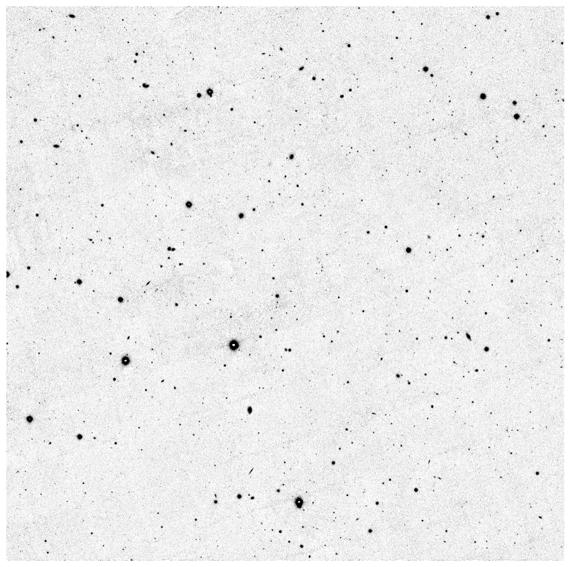
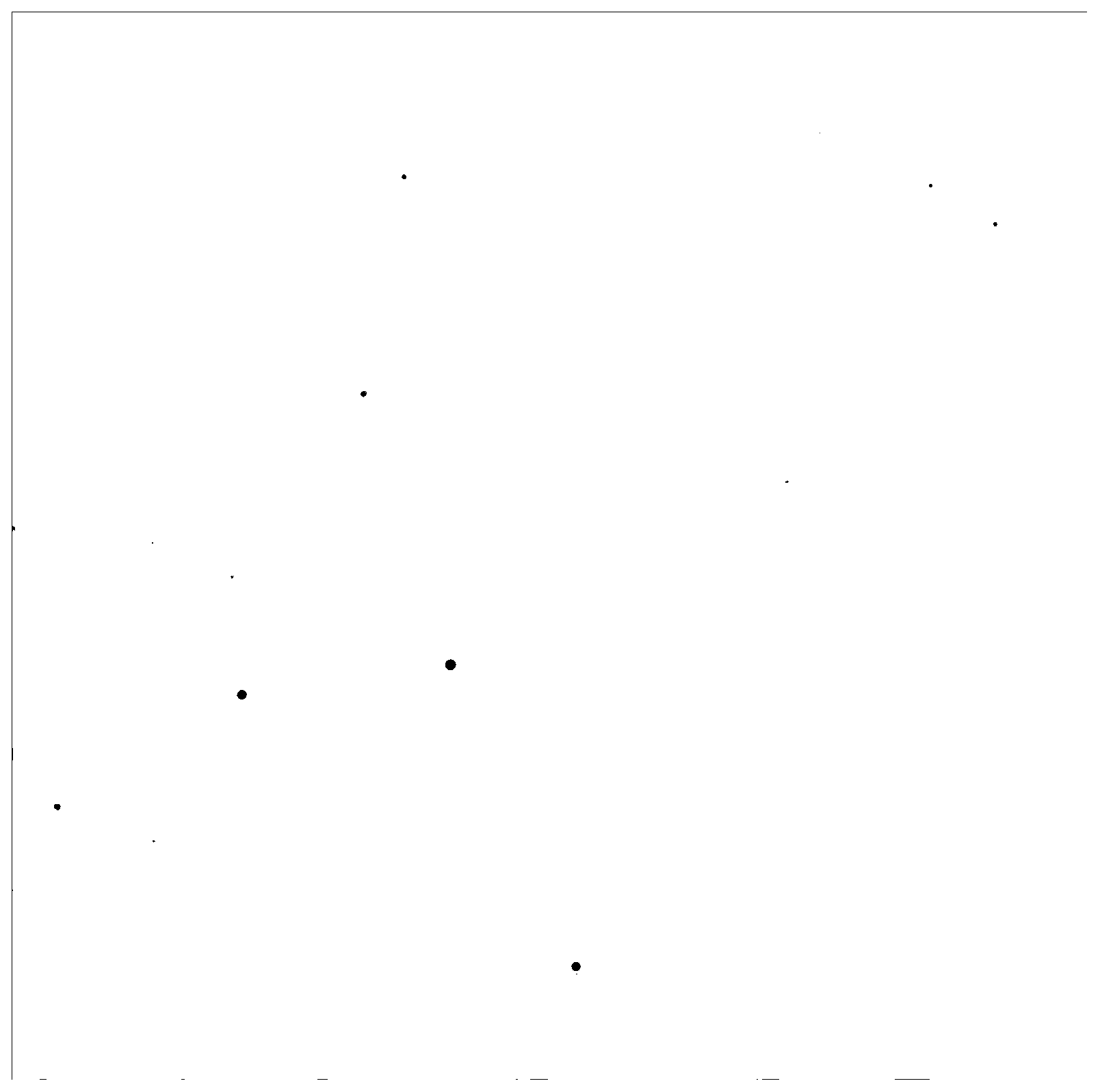
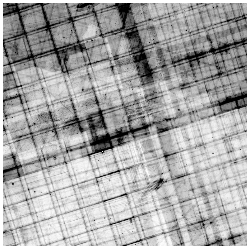
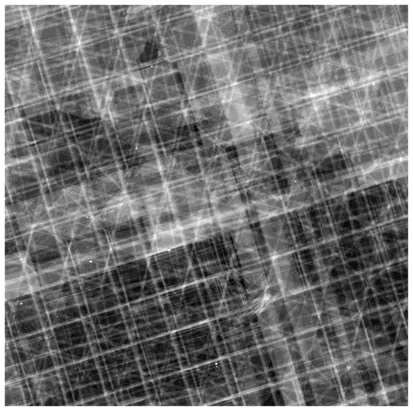
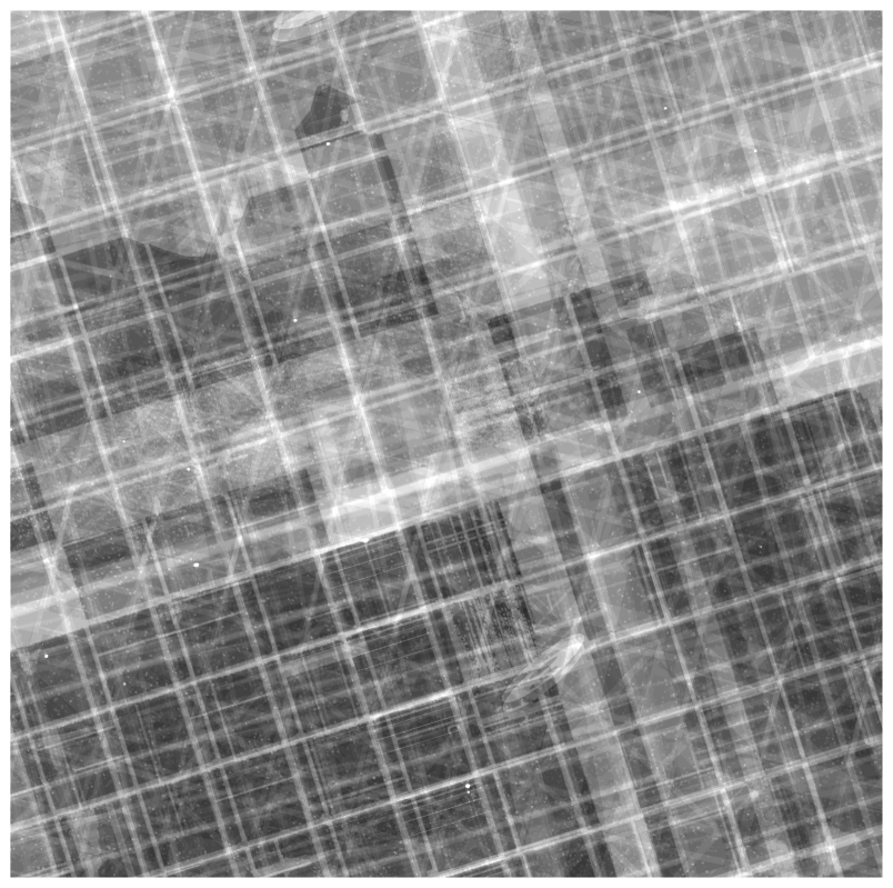
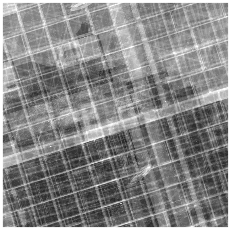
7. Difference Images

The image matching process used in constructing difference images is essentially the same as for the stacking process. An image is chosen as a template, another image as the input, and after matching sources to determine the scaling and transparency, convolution kernels are defined that are used to convolve one or both of the images to a target PSF. The images are then subtracted, and as they should now share a common PSF, static sources are largely subtracted (completely in an ideal case), whereas sources that are not static between the two images leave a significant remnant. More information on the difference image construction is contained in Price et al. (2017). The following section contains an overview of the difference image construction used for the data in DR2.

The images used to construct difference images can be either individual warp skycell frames or stacked images, with support for either to be used as the template or input. In general, for differences using stacks, the deepest stack (or the only stack in the case of a warp-stack difference) is used as the template. The PV3 processing used warp-stack differences of all input warps against the stack that was constructed from those inputs. The same ISIS kernels as were used in the stack image combination were again used to match the stack PSF to the input warp PSF. After convolution of the image products, the difference is constructed for both the positive (warp minus stack) and inverse (stack minus warp) to allow for the photometry of the difference image to detect sources that both rise and fall relative to the stack. The convolution process grows the mask fraction of pixels relative to the warp (the largest source of masked pixels in these warp stack differences). Any pixel that after convolution has any contribution from a masked pixel is masked as well, ensuring only fully unmasked pixels are used.

For warp-warp differences, such as those used for the ongoing Solar System moving object search in nightly observations (Denneau et al., 2013), the warp that was taken first is used as the template. As there is less certainty in which of the two input images will have better seeing, a “dual” convolution method is used. Both inputs are convolved to a target PSF that is not identical to either input. This intermediate target is essential for the case in which the PSFs of the two inputs have been distorted in orthogonal directions. Simply convolving one to match the other would require some degree of deconvolution along one axis. As this convolution method by necessity uses more free parameters, the ISIS kernels used are chosen to be simpler than those used in the warp-stack differences. The ISIS widths are kept the same (1.5, 3.0, 6.0 pixel FWHMs), but each Gaussian kernel is constrained to only use a second-order polynomial. As with the warp-stack differences, the mask fraction grows between the input warp and the final difference image due to the convolution. For the warp-warp differences, each image mask grows based on the appropriate convolution kernel, so the final usable image area is highly dependent on ensuring that the telescope pointings are as close to identical as possible. The observing strategy to enable this is discussed in more detail in Chambers et al. (2017).

8. Future Plans

Although the detrending and image combination algorithms work well to produce consistent and calibrated images, having the PV3 processing of the full $3\pi$ data set allows issues to be identified and solutions created for future improvements to the IPP pipeline. In addition, the existence of the final calibrated catalog can be used to look for issues that appear dependent on focal plane position.

One obvious way to make use of the PV3 catalog is to do a statistical search for electronic crosstalk ghosts that do not match a known rule. Given that bright stars do not equally populate all fields, choosing exposures to examine to look for crosstalk rules is difficult. The current crosstalk rules were derived from expectations based on the detector engineering, supplemented by rules identified largely based on unmatched transients. With the full catalog, identification of new rules can be done statistically, looking at detection pairs that appear more often than random.

There is some evidence that we have not fully identified all of these crosstalk rules, based on a study of PV3 images. For example, extremely bright stars may be able to create crosstalk ghosts between the second cell column of OTA01 and OTA21, with possibly fainter ghosts appearing on OTA11. Despite the symmetry observed in the main ghost rules, there do not appear to be clear examples of a similar ghost between OTA47 and OTA66. Examining this further based on the PV3 catalog should provide a clear answer to this, as well as clarify brightness limits below which the ghost does not appear.

The PV3 catalog may also allow better determination of which date ranges we should use to build the dark model. The date ranges currently in use are based on limited sampling of exposures, and do not have strong tests indicating that they are optimal. By examining the scatter between the detections on a given exposure and the catalog average, we can attempt to look for increases in scatter that might suggest that the dark model used is not completely correcting the camera. Looking at this based on the catalog would allow this information to be generated without further image level processing.

In addition to improving the quality of the catalog for any future reprocessing, there are a number of possible improvements that could fix the image cosmetics. A study of the burntool fits on stars that have been badly saturated suggest that we may be able to improve the trail fits by considering not the star center, but rather the edge of saturation. This restricts the fit to only consider the data along the trail, and may improve the fit quality. Implementing this change would require additional bookkeeping of which pixels were saturated, as the fits on subsequent exposures will need to skip these pixels before fitting the persistence trail. This is unlikely to seriously impact the photometry of objects, but may improve the results of stacks if fewer pixels need to be rejected.

The fringe model used currently is based on only a limited number of days of data. This means that the model calculated may not be fully sensitive to the exact spectrum of the sky. This may make the model quality differ based on the date and local time of observation. There is some evidence that the fringe model does fit some dates better than others, and so improving this by expanding the number of input exposures may improve a wider range of dates.

Finally, a large number of issues arise due to the row-to-row bias issues. The PATTERN.ROW correction is used on a limited number of cells, to minimize any possible distortion of bright stars or dense fields by the fitting process. As the row-to-row bias changes very quickly in the y pixel axis and slowly along the x, it may be possible to isolate and remove this signal in the Fourier domain. Preliminary investigations have shown that there is a small peak visible in the power spectrum of a single cell, but determining the best way to clip this peak to reduce the noise in the image space is not clear.

9. Conclusion

The Pan-STARRS1 PV3 processing has reduced an unprecedented volume of image data, and has produced a catalog for the $3\pi$ Survey containing hundreds of billions of individual measurements of three billion astronomical objects. Accurately calibrating and detrending is essential to ensuring the quality of these results. The detrending process detailed here produces consistent data, despite the many individual detectors and their individual response functions.

From these individual exposures, we are able to construct images on common projections and orientations, further removing the particulars of any single exposure. Furthermore, by created stacked images, we can determine an estimate of the true static sky, providing a deep data set that is ideal for use as a template for image differences.

The Pan-STARRS1 Surveys (PS1) have been made possible through contributions by the Institute for Astronomy, the University of Hawaii, the Pan-STARRS Project Office, the Max-Planck Society and its participating institutes, the Max Planck Institute for Astronomy, Heidelberg and the Max Planck Institute for Extraterrestrial Physics, Garching, The Johns Hopkins University, Durham University, the University of Edinburgh, the Queen’s University Belfast, the Harvard-Smithsonian Center for Astrophysics, the Las Cumbres Observatory Global Telescope Network Incorporated, the National Central University of Taiwan, the Space Telescope Science Institute, and the National Aeronautics and Space Administration under Grant No. NNX08AR22G issued through the Planetary Science Division of the NASA Science Mission Directorate, the National Science Foundation Grant No. AST-1238877, the University of Maryland, Eotvos Lorand University (ELTE), and the Los Alamos National Laboratory.

References

- Alard (2000) Alard, C. 2000, A&AS, 144, 363
- Alard & Lupton (1998) Alard, C. & Lupton, R. H. 1998, ApJ, 503, 325
- Chambers et al. (2017) Chambers, K. C., Magnier, E. A., Metcalfe, N., & et al. 2017, ArXiv e-prints
- Denneau et al. (2013) Denneau, L., Jedicke, R., Grav, T., Granvik, M., Kubica, J., Milani, A., Vereš, P., Wainscoat, R., Chang, D., Pierfederici, F., Kaiser, N., Chambers, K. C., Heasley, J. N., Magnier, E. A., Price, P. A., Myers, J., Kleyna, J., Hsieh, H., Farnocchia, D., Waters, C., Sweeney, W. H., Green, D., Bolin, B., Burgett, W. S., Morgan, J. S., Tonry, J. L., Hodapp, K. W., Chastel, S., Chesley, S., Fitzsimmons, A., Holman, M., Spahr, T., Tholen, D., Williams, G. V., Abe, S., Armstrong, J. D., Bressi, T. H., Holmes, R., Lister, T., McMillan, R. S., Micheli, M., Ryan, E. V., Ryan, W. H., & Scotti, J. V. 2013, PASP, 125, 357
- Flewelling et al. (2016) Flewelling, H. A., Magnier, E. A., Chambers, K. C., Heasley, J. N., Holmberg, C., Huber, M. E., Sweeney, W., Waters, C. Z., Chen, T., Farrow, D., Hasinger, G., Henderson, R., Long, K. S., Metcalfe, N., Nieto-Santisteban, M. A., Norberg, P., Saglia, R. P., Szalay, A., Rest, A., Thakar, A. R., Tonry, J. L., Valenti, J., Werner, S., White, R., Denneau, L., Draper, P. W., Jedicke, R., Kudritzki, R.-P., Price, P. A., Chastel, S., McClean, B., Postman, M., & Shiao, B. 2016, ArXiv e-prints
- Hodapp et al. (2004) Hodapp, K. W., Siegmund, W. A., Kaiser, N., Chambers, K. C., Laux, U., Morgan, J., & Mannery, E. 2004, in Proc. SPIE, Vol. 5489, Ground-based Telescopes, ed. J. M. Oschmann, Jr., 667–678
- Huber et al. (2017) Huber, M., TBD, A., TBD, B., & et al. 2017, ArXiv e-prints
- Lanczos (1956) Lanczos, C. 1956, Applied analysis, Prentice-Hall mathematics series (Prentice-Hall)
- Lupton et al. (1999) Lupton, R. H., Gunn, J. E., & Szalay, A. S. 1999, AJ, 118, 1406
- Magnier & Cuillandre (2004) Magnier, E. A. & Cuillandre, J.-C. 2004, PASP, 116, 449
- Magnier et al. (2017) Magnier, E. A., Schlafly, E. F., Finkbeiner, D. P., & et al. 2017, ArXiv e-prints
- Magnier et al. (2016a) Magnier, E. A., Schlafly, E. F., Finkbeiner, D. P., Tonry, J. L., Goldman, B., Röser, S., Schilbach, E., Chambers, K. C., Flewelling, H. A., Huber, M. E., Price, P. A., Sweeney, W. E., Waters, C. Z., Denneau, L., Draper, P., Hodapp, K. W., Jedicke, R., Kudritzki, R.-P., Metcalfe, N., Stubbs, C. W., & Wainscoast, R. J. 2016a, ArXiv e-prints
- Magnier et al. (2016b) Magnier, E. A., Sweeney, W. E., Chambers, K. C., Flewelling, H. A., Huber, M. E., Price, P. A., Waters, C. Z., Denneau, L., Draper, P., Jedicke, R., Hodapp, K. W., Kudritzki, R.-P., Metcalfe, N., Stubbs, C. W., & Wainscoast, R. J. 2016b, ArXiv e-prints
- Onaka et al. (2008) Onaka, P., Tonry, J. L., Isani, S., Lee, A., Uyeshiro, R., Rae, C., Robertson, L., & Ching, G. 2008, in Proc. SPIE, Vol. 7014, Ground-based and Airborne Instrumentation for Astronomy II, 70140D
- Price et al. (2017) Price, P. A., TBD, A., TBD, B., & et al. 2017, ArXiv e-prints
- Schlafly et al. (2012) Schlafly, E. F., Finkbeiner, D. P., Jurić, M., Magnier, E. A., Burgett, W. S., Chambers, K. C., Grav, T., Hodapp, K. W., Kaiser, N., Kudritzki, R.-P., Martin, N. F., Morgan, J. S., Price, P. A., Rix, H.-W., Stubbs, C. W., Tonry, J. L., & Wainscoat, R. J. 2012, ApJ, 756, 158
- Tonry & Onaka (2009) Tonry, J. & Onaka, P. 2009, in Advanced Maui Optical and Space Surveillance Technologies Conference, E40
- Tonry et al. (2012) Tonry, J. L., Stubbs, C. W., Lykke, K. R., Doherty, P., Shivvers, I. S., Burgett, W. S., Chambers, K. C., Hodapp, K. W., Kaiser, N., Kudritzki, R.-P., Magnier, E. A., Morgan, J. S., Price, P. A., & Wainscoat, R. J. 2012, ApJ, 750, 99
- Wainscoat et al. (2015) Wainscoat, R., Weryk, R., Schunova, E., & Carter Chambers, K. 2015, IAU General Assembly, 22, 2251124