Trident: a universal tool for generating synthetic absorption spectra
from astrophysical simulations

Abstract

Hydrodynamical simulations are increasingly able to accurately model physical systems on stellar, galactic, and cosmological scales; however, the utility of these simulations is often limited by our ability to directly compare them with the datasets produced by observers: spectra, photometry, etc. To address this problem, we have created trident, a Python-based, open-source tool for post-processing hydrodynamical simulations to produce synthetic absorption spectra and related data. trident can (i) create absorption-line spectra for any trajectory through a simulated dataset mimicking both background quasar and down-the-barrel configurations; (ii) reproduce the spectral characteristics of common instruments like the Cosmic Origins Spectrograph; (iii) operate across the ultraviolet, optical and infrared using customizable absorption line lists; (iv) trace simulated physical structures directly to spectral features; (v) approximate the presence of ion species absent from the simulation outputs; (vi) generate column density maps for any ion; and (vii) provide support for all major astrophysical hydrodynamical codes. trident was originally developed to aid in the interpretation of observations of the circumgalactic medium (CGM) and intergalactic medium (IGM), but it remains a general tool applicable in other contexts.

1. Introduction

1.1. Why observe simulated data?

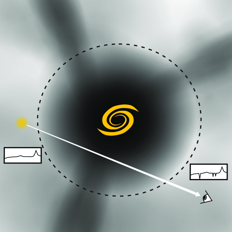
Most of the baryonic material in the universe consists of low-density gas insufficiently bright to be detected by its emission alone (e.g., Cen et al., 1994; Zhang et al., 1995; Miralda-Escudé et al., 1996; Hernquist et al., 1996; Davé et al., 2001). In order to reveal this gas, observers rely on its ability to absorb certain wavelengths of light from bright background sources, like how the sun appears red to viewers looking at it through an Earth-bound dust cloud. The location of a background source in the sky thus defines a sightline, usually parameterized as an infinitesimally thin one-dimensional line, that probes the intervening material between us and the background object. Electron energy transitions in the intervening gas preferentially absorb light at discrete wavelengths, creating troughs in the spectrum of the light along this sightline. The atoms and ions present in the intervening gas determine the viable electron transitions, which when coupled with the relative velocity to the observer, produce the distribution of absorption-line features in the observed spectrum. Thus, the characteristics of different absorption features in a sightline’s spectrum can reveal an enormous amount of information about the density, temperature, velocity, radiation field, and ionic composition of gas along a given line of sight. See Figure 1 for a schematic of this process.

Figure 1.— Schematic showing how absorption line spectroscopy indicates the presence of low-density gas through its absorption of light from background objects. Ions in the intervening gas between an observer and a bright background object absorb discrete wavelengths of light providing information about the composition and phase of the intervening gas. Here, an observer detects absorption from the CGM (inside dashed circle) and filamentary IGM (outside dashed circle) in the spectrum from a background quasar.

“Absorption-line spectroscopy” is employed in a variety of environments where observers attempt to detect low-density gas, ranging from the gas between stars (interstellar medium – ISM), the gas surrounding galaxies (circumgalactic medium – CGM), and the gas between galaxies (intergalactic medium – IGM). These observations provide us with clues as to (i) how galaxies balance external gas accretion (e.g. Rubin, 2016; Lehner, 2016) with turbulent outflows of material from supernovae (e.g. Hummels & Bryan, 2012; Fielding et al., 2016) and supermassive black holes (e.g. Kacprzak et al., 2015; Johnson et al., 2015); (ii) what is happening in the vast volume of “empty” space between galaxies (e.g. Peeples et al., 2013); and (iii) what can the CGM/IGM tell us about the evolution of the universe as a whole (e.g. McQuinn, 2016).

Observers require that background sources used in absorption-line spectroscopy be sufficiently bright and well-characterized, so that the baseline spectra are constrained when identifying absorption features due to intervening material. Typically, quasars are used as background sources, but because bright quasars are relatively uncommon, few cosmic structures such as galaxies or gas filaments can be probed by multiple sightlines. Thus in order to study these gas structures, observers must combine samples of sightlines through many different galaxies, making assumptions about the homogeneity of the probed galaxy population in order reach general conclusions (e.g. cos-halos – Tumlinson et al., 2013; cos-dwarfs – Bordoloi et al., 2014; KBSS – Rudie et al., 2012, Steidel et al., 2010, Chen et al., 2010, Prochaska et al., 2011, Nielsen et al., 2013, Liang & Chen, 2014, Rubin et al., 2014, Turner et al., 2015). These samples contain an enormous amount of information about the galaxy population, but as of yet, the details of the relationship between the CGM and host galaxy are not well understood.

In the last decade, significant advances have occurred in the field of hydrodynamical modeling of astrophysical systems. There now exist many high-resolution simulations that track the positions and velocities of stars as well as the phase and composition of gas through galaxies and significant cosmological volumes (e.g. eris – Guedes et al., 2011; fire – Hopkins et al., 2014a; illustris – Vogelsberger et al., 2014; eagle – Schaye et al., 2015). These simulations possess sufficient detail to follow the distribution and evolution of individual gas, metal, and ionic species self-consistently, making them ideal aids in understanding what is truly happening in the low-density gas so difficult to track observationally.

The best way to compare observations and simulations is to directly compare similar data products. The production of synthetic observations of simulated datasets enables such a comparison by modeling the way light travels through space and into telescopes. Astrophysics has a rich history in producing mock spectra in many contexts including stars (e.g. Kurucz, 1979), the Sun (e.g. Husser et al., 2013), galaxies (e.g. starburst99 – Leitherer et al., 1999), stellar population synthesis (e.g. fsps – Conroy et al., 2009), molecular clouds (e.g. radmc-3d – Dullemond, 2012), plasmas (e.g. cloudy – Ferland et al., 1998), and dust (e.g. dusty – Nenkova et al., 2000). Additionally, there exist a number of open-source, Monte Carlo radiative transfer codes (e.g. sunrise – Jonsson, 2006; hyperion – Robitaille, 2011) that are potentially applicable to synthetic absorption-line spectroscopy, but they currently lack line transfer physics necessary to produce absorption features.

A number of works have made use of specialized tools for generating synthetic spectra from simulation data, each designed with the specific features and needs of their own data formats in mind. Examples include specexbin (Oppenheimer & Davé, 2006) and specwizard (Schaye et al., 2003) for gadget (Springel et al., 2001; Springel, 2005); the method of Shen et al. (2013) for gasoline (Wadsley et al., 2004); the tools of Churchill et al. (2015) and Liang et al. (2016) for their specific versions of art (Kravtsov et al., 1997; Kravtsov, 1999); the methods of Smith et al. (2011) and Hummels et al. (2013) (early versions of the work presented here) for enzo (Bryan et al., 2014); and the fake_spectra code (Bird et al., 2015) for arepo (Springel, 2010). These tools span a range of simulation methodologies, from adaptive mesh-refinement (AMR) to smoothed-particle hydrodynamics (SPH) and moving mesh techniques, and so must work with fundamentally different quantities.

Thus, there is a need for a universal tool for generating mock absorption-line spectra, one that can work with many different simulation code formats. Like a real telescope facility, this virtual telescope is most beneficial when it is publicly available, not used solely by its designers and their collaborators. Such a publicly available, universal tool prevents unnecessary duplication of efforts, provides a single resource for members of the scientific community to contribute their specific strengths, ensures fewer bugs and more features, and enables inter-code simulation comparison efforts (e.g. agora project – Kim et al., 2014).

1.2. Introducing trident

This paper announces the full public release of trident, an open-source tool for generating synthetic absorption spectra from astrophysical hydrodynamical simulations. trident is an object-oriented, pure Python library with support for both Python 2 and Python 3. trident relies on the ability of the yt analysis toolkit (Turk et al., 2011) to ingest simulation data from a vast array of sources and formats for further analysis and processing. As a result, trident is capable of generating spectra for at least 10 different simulation codes. In addition to spectral creation, trident provides other analysis tools, such as a method for creating fields of ion densities (e.g., C IV, O VI, etc.) from simulation data using various photo- and collisional ionization models. trident can also operate in parallel using the message passing interface system (mpi, Forum, 1994) to scale to many processors and speed up execution (See Appendix A for details).

Members of the scientific community are actively encouraged to use and develop trident as a community code according to the Revised BSD License. Table 1 lists locations for various important resources related to trident including its documentation, mailing list, and source code repository.

This paper is composed as follows. Section 2 describes the three-pronged approach trident takes to generating spectra: creating ion fields for the simulation dataset (Section 2.2), making sightlines through the dataset to sample the relevant fields (Section 2.3), and depositing absorption lines based on the characteristics of gas along the sightline (section 2.4). Section 3 provides an annotated Python script demonstrating the use of trident to create a simple spectrum. In Section 4, we perform some tests of trident including a comparison with observational data and a curve-of-growth analysis, and we describe some of trident’s assumptions and limitations. Finally, Section 5 summarizes the highlights and features of the code.

Resource	Location
Web Page	http://trident-project.org
Source Code	https://github.com/trident-project/trident
Documentation	http://trident.readthedocs.org
Mailing List	trident-project-users@googlegroups.com

Table 1Important Trident Resources

2. Code Methodology

This section describes the algorithms employed by trident to post-process simulation outputs. It covers a brief discussion of: what simulation outputs contain and how trident interacts with them (Section 2.1); how trident estimates the concentration of a desired ion when absent from the simulation (Section 2.2); how trident calculates the trajectory of different sightlines (Section 2.3); how trident produces an absorption-line spectrum (Section 2.4); and how trident processes that spectrum to resemble real observations (Section 2.5).

trident is an object-oriented software library with its own set of classes and modules. The most important of these are discussed in detail in later sections, but they are provided here as a reference:

• ion_balance – a module used to calculate the density of any atomic ion in a simulated dataset

• LightRay – a class describing a one-dimensional sightline through a simulated dataset

• SpectrumGenerator – a class responsible for creating absorption line spectra from LightRay objects

For a full description of all classes and their usage in trident, see the API documentation.

2.1. Brief overview of simulation outputs and how trident and yt interact with them

An astrophysical hydrodynamical simulation output represents a three-dimensional volume with a series of scalar and vector fields expressing different fluid quantities for the gas across that volume. Grid codes discretize the gas into a regular grid with elements of fixed volume, oftentimes employing AMR to achieve higher resolution in regions of interest. SPH codes discretize the gas into particles, each representing a parcel of gas with fixed mass, which can be smoothed using a three-dimensional smoothing kernel to achieve a finite size. Moving mesh and meshless codes take a hybrid approach by representing the gas over tessellating fluid elements that change shape as the gas moves. Despite their differences, in all of these code formats the gas is represented as a series of field elements describing its distribution in position, velocity, density, temperature, metallicity, etc.

Code	Type	Reference
arepoa	Moving Mesh	Springel (2010)
art-i	AMR	Kravtsov (1999)
art-ii	AMR	Rudd et al. (2008)
athena	AMR	Stone et al. (2008)
changa	SPH	Stinson et al. (2006)
enzo	AMR	Bryan et al. (2014)
flash	AMR	Fryxell et al. (2000)
gadget	SPH	Springel (2005)
gasoline	SPH	Wadsley et al. (2004)
gizmo	SPH & Meshless	Hopkins (2015)
ramses	AMR	Teyssier (2002)
ain development

Table 2Simulation codes that trident explicitly supports.

trident was originally developed as an analysis module within the yt framework (Turk et al., 2011), and consequently it inherits the way yt interacts with simulation outputs. For operations that involve sampling fluid values at arbitrary locations, particle fields must be converted to a grid-like structure. yt first creates an underlying octree grid structure that ensures high resolution in regions of high particle density, and then deposits particle-based fluid quantities on to these grid elements using the appropriate smoothing kernel and length. These steps ensure that subsequent analysis can be treated homogeneously across different simulation formats and methods. Note that some operations like calculating ion densities are performed on the particles prior to the smoothing process.

Because of trident’s close relationship to yt, many of the features that trident provides to users, such as the ability to post-process a dataset to include density fields for a desired ion, can be further used within the yt framework seamlessly. This enables users to make volumetric projections and slices of these ion fields, create phase plots and probability distribution functions for the presence of arbitrary ions, categorize how fluid quantities change along a line of sight, and more.

In addition, trident inherits yt’s support for every major astrophysical hydrodynamical code. Table 2 contains a list of the simulation codes that have been tested and confirmed to work with trident. trident should function correctly with other yt-supported codes, but appropriate sample datasets were unavailable for testing.

Figure 2.— Operation of trident’s ion_balance module. Grid and particle datasets pass their redshift and fluid quantities (density, temperature, metallicity) to the ion_balance module to estimate the number density of any ions of interest (e.g. H I, C IV, O VI). These number densities are computed on the original fluid elements, whether grid cell or particle. Additionally, particle-based datasets are deposited onto a grid as an AMR octree using the particle smoothing kernel.

2.2. Creating ion fields with the ion_balance module

In order to create absorption lines for a given ion, it is necessary that a fluid field representing the density of that ion be present for all computational elements sampled by the sightline or LightRay. In some cases, these fields may be explicitly tracked by the simulation with a non-equilibrium chemistry solver. Examples of this include Smith et al. (2011) and Hummels et al. (2013), which follow atomic species of H and He in non-equilibrium, and Cen & Fang (2006), which additionally follows O V through O IX. However, in most cases, tracking additional ion densities within a simulation is computationally prohibitive, and so they must be derived from the available data fields using models that assume ionization equilibrium.

For species not followed by the simulation, trident’s ion_balance sub-package creates a new field by defining the density of ion, $i$, of element, $X$ as

$$n_{X_{i}}=n_{X}\ f_{X_{i}},$$ (1)

where $n_{X}$ is the total number density of the element and $f_{X_{i}}$ is the ionization fraction of the $i$’th ion. For simulations that track multiple metal fields, such as those presented by Hopkins et al. (2014b), $n_{X}$ may already exist in the simulation output. If this is not the case, then ion_balance defines $n_{X}$ as

$$n_{X}=n_{H}\ Z\ \left(\frac{n_{X}}{n_{H}}\right)_{\odot},$$ (2)

where $n_{H}$ is the total hydrogen number density, $Z$ is the metallicity and $(n_{X}/n_{H})_{\odot}$ is the solar abundance by number. If the simulation does not explicitly track the hydrogen number density, we assume it to be given as

$$n_{H}=\chi\frac{\rho}{m_{H}},$$ (3)

where $\rho$ is the total gas density and $\chi$ is the primordial H mass fraction, for which we adopt a value of 0.76. If desired, ion_balance can overwrite a dataset’s existing ion fields using the force_override keyword to ensure consistency in ionization calculations.

Figure 3.— Projections of a 1536³ cosmological enzo dataset aimed at probing the nature of the intergalactic medium, similar to those presented by Smith et al. (2011). Each projection shows a region of the box that is 30 Mpc on a side and 5 Mpc deep. The region is centered on a halo in the simulation that was identified using the rockstar halo-finder Behroozi et al. (2012). The halo has a mass of $1.9~{}\times~{}10^{14}~{}\rm M_{\odot}$ and a virial radius of $1.5$ Mpc. From top to bottom, the left panels show density, temperature, and metallicity, while the right panels show the projected number densities (effective column densities) of H I, C IV, and O VI. The ion number densities were computed using the ion_balance module in trident.

Under the assumption of ionization equilibrium, the ionization fraction is a function of temperature, density, and the shape and intensity of the incident radiation field. Currently, ion_balance only considers radiation from metagalactic UV background models, such as those of Faucher-Giguère et al. (2009) and Haardt & Madau (2012). In these models, the radiation field is parameterized solely by the value of the redshift, making the ionization fraction a function of just temperature, density, and redshift. Using the code in Smith et al. (2008), we have computed the equilibrium ionization fractions for all the ions and elements through atomic number 30 (i.e., Zn) over a grid of temperature, hydrogen number density, and redshift. These data are generated with a series of single zone simulations using the photo-ionization software, cloudy (Ferland et al., 2013), following the same method used by the grackle chemistry and cooling library (Smith et al., 2016). The resulting data are saved as a three-dimensional lookup table, which is loaded by trident when needed. Ionization fractions for each ion are then calculated for each computational element by linearly interpolating over these pre-computed tables. Currently, trident provides data tables for the UV backgrounds described by Faucher-Giguère et al. (2009) and Haardt & Madau (2012), but the method is general enough that other backgrounds can be added. For more information demonstrating the accuracy of these tables, see Appendix B.

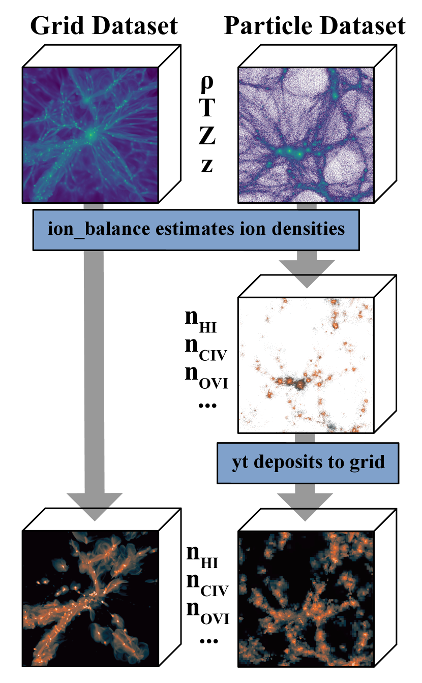
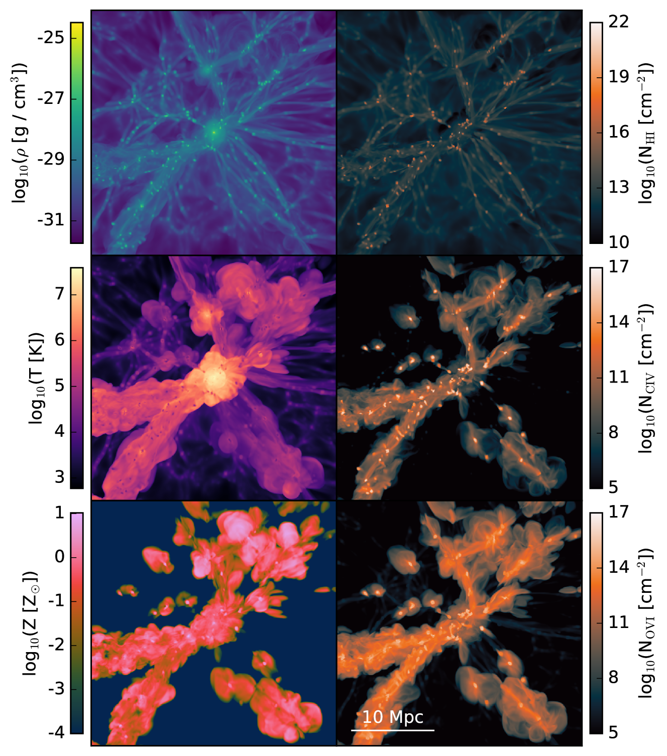
Figure 2 presents a visual illustration of the way in which the ion_balance module generates ion fields for simulated datasets. ion_balance can create ion density fields for all computational elements for which density and temperature fields exist. This allows fields created by ion_balance to be used independently of spectrum generation, for example, to study the spatial distribution of various ions and their relationship to physical gas quantities, as shown in Figure 3. When creating light rays from grid-based simulation data, the creation of the ion fields is saved for after the light ray is generated, allowing the fields to only be created for the cells in the light ray itself and not the entire simulation domain. Since the three-dimensional interpolation can be computationally expensive when performed for all grid cells in the domain, this results in a significant speedup. However, for particle-based datasets, where particle fields are smoothed onto a grid, we do not take this shortcut. In this case, we first create the ion fields for each particle on the particle itself, and afterward deposit the resulting ion densities onto the corresponding grid cells according to the chosen smoothing kernel. While more time consuming, this avoids errors that may arise by creating ion fields from smoothed density and temperature fields.

2.3. Sightline creation: the LightRay object

The next step in the process of generating a spectrum is choosing and sampling a line of sight through the simulation data. The user specifies the trajectory of the sightline through the simulation output, as well as the gas fields they wish to sample. Optionally, the user can specify which spectral lines or ionic species it wishes to include in any subsequently generated spectrum, and trident will include the necessary fields. The end product of this step is a LightRay object, a set of spatially-ordered, one-dimensional arrays sampling the the desired fields of the simulation output along the ray’s path. The LightRay is saved to an hdf5 file (The HDF Group, 1997–) that can be reloaded by yt as an ordinary dataset for the purposes of spectrum generation or direct access for further analysis.

These “light rays” make use of yt’s ray data container, which takes a start and end point and returns field values for all computational elements intersected by the ray’s trajectory through the dataset. For grid-based simulation codes, these computational elements are simply the highest-resolution grid cells of the Eulerian mesh along the line of sight. As described in Section 2.1, particle-based codes have their particles deposited to a grid by first smoothing the particles into an octree mesh to create gridded, Eulerian fluid fields. In this case, the computational elements returned by the LightRay are these octree cells.

In addition to sampling the fields specified by the user, the LightRay creates some special fields for further processing. For each line element along the LightRay, trident calculates and records its: dl – path length; dredshift – cosmological redshift interval; redshift – cosmological redshift; velocity_los – line of sight velocity; redshift_dopp – doppler redshift; and redshift_eff – effective redshift. Here we derive all of these quantities.

Figure 4.— The methods by which LightRay objects are generated to represent a sightline path from point $a$ to point $b$ (the observer). Left: Simple rays are defined by a start point and end point for a single dataset output. Right: Compound rays contain path lengths longer than the width of a single dataset by continuing the ray path over periodic boundary conditions and consecutive outputs.

Let us define the sightline of a LightRay vector $\vec{l}$ passing through a single dataset from point $a$ to point $b$ where the observer sits at point $b$. We can think of it as a collection of $n$ individual line elements $d\vec{l}$:

$$\vec{l}=\vec{r}_{b}-\vec{r}_{a}=\sum_{i=0}^{n}{d\vec{l}_{i}}$$ (4)

Field values along the light ray are the values within the grid or octree cell intersected by the ray’s trajectory. The path length, $d\vec{l}_{i}$, is the vector intersection of the ray with the cell.

$$dl_{i}=|d\vec{l}_{i}|$$ (5)

We assume a smooth Hubble expansion between points $a$ and $b$ in the ray such that their separation in redshift is given by the comoving radial distance (Hogg, 1999), given by

$$l=D_{H}\int_{z_{a}}^{z_{b}}\frac{dz^{\prime}}{E(z^{\prime})},$$ (6)

where

$$E(z)=\sqrt{\Omega_{M}(1+z)^{3}+\Omega_{k}(1+z)^{2}+\Omega_{\Lambda}},$$ (7)

$D_{H}$ is the Hubble distance, and $\Omega_{M}$, $\Omega_{k}$, and $\Omega_{\Lambda}$ are the ratios of mass density, spatial curvature density, and vacuum density, respectively, to the critical density of the universe. Since the simulation data provide $l$, the comoving radial distance between $a$ and $b$, and we require $z_{b}-z_{b}$, the redshift difference between $a$ and $b$, we must invert equation 6. Since there is no simple analytical form, we use Newton’s method to iteratively calculate the redshift interval between the points, taking the redshift of the simulation as the redshift at the far point $a$.

Now that we know the redshift interval connecting points $a$ and $b$ within our simulation output, we assume a line element’s cosmological redshift interval is linearly related to its path length:

$$dz_{i}=\frac{dl_{i}}{l}(z_{b}-z_{a})$$ (8)

This redshift interval estimate is a good approximation on the small path lengths within an individual dataset. This also allows us to calculate the cosmological redshift for the $i$’th LightRay element as:

$$z_{i}=z_{b}+\sum_{j=i}^{n}dz_{j}$$ (9)

When generating spectra, the observer cannot discern between absorber redshifts due to cosmological expansion and its relative motion along the line of sight. Thus, by default, trident also includes the effects of doppler redshift due to radial motions of the gas. The line of sight velocity for a LightRay element is defined as:

$$v_{LOS,i}=\vec{v}_{i}\cdot d\vec{l}_{i}=v_{i}dl_{i}\cos(\theta_{i})$$ (10)

where $v_{i}$ is the local gas velocity field in the cell and $\theta_{i}$ is the angle between the line of sight and the gas velocity vector. The local velocity field enables us to calculate a LightRay element’s doppler redshift $z_{dopp,i}$ as

$$1+z_{dopp,i}=\frac{1+\frac{v_{i}}{c}\ cos(\theta_{i})}{\sqrt{1-\left(\frac{v_{i}}{c}\right)^{2}}},$$ (11)

where $c$ is the speed of light. The effective redshift, the redshift used to modify the location of spectral absorption lines, for each element of the ray is then given as a combination of its cosmological and doppler redshifts (Peebles, 1993) as:

$$1+z_{eff,i}=(1+z_{dopp,i})\ (1+z_{i}).$$ (12)

LightRay generation is divided into two use cases, simple rays and compound rays. Aside from the differences in generating their trajectories, these objects have similar internal structures and are treated the same by the rest of the trident machinery.

2.3.1 Simple rays: rays traversing a single dataset

Simple rays are defined for use with a single simulation output at a fixed point in time. The primary use case for simple rays is the creation of spectra from targeted physical structures, such as a specific galaxy at a particular redshift. To generate a simple ray, the user must specify the simulation output dataset and the starting and ending locations of the ray in the dataset volume. trident uses the simulation dataset’s redshift as the redshift at the back of the ray (location $a$), and increments it forward along its path to the user according to the method described in equations 6-8. For non-cosmological simulation outputs, trident defaults to using a redshift of zero, but the user can specify any desired value. Figure 4 illustrates a simple ray object traversing a simulation dataset.

Figure 5.— Physical structures traced to spectral features as trident generates a spectrum. Begin at the top and travel downward A-G, noting vertical alignment between plots. A: A 2D slice in neutral hydrogen density taken from a low-resolution simulation of some cosmological filaments. Black arrows represent the gas velocities, and a white arrow indicates the 10 Mpc-long LightRay sightline passing through the slice to the observer on the left. B: Individual points represent gas cells probed by the sightline, plotted as cosmological redshift versus neutral hydrogen column density. C: Line of sight velocity for each gas cell along the LightRay. D: Applying a doppler shift from the line of sight velocity shifts the location of each gas absorber into effective redshift, the frame of the observer. E: In this new effective redshift frame, equivalent to $(1+z)1216\AA$ for the Lyman-$\alpha$ transition, the temperature of each gas cell is plotted versus observed wavelength. F: Points indicate the H I column density in this effective redshift frame with thermal widths determined from gas temperature denoted as red error bars. G: Voigt profiles calculated for each gas cell for the Lyman-$\alpha$ transition in green, superimposing to the black profile, the spectral feature seen by the observer.

2.3.2 Compound rays: rays traversing multiple datasets

Synthetic spectra that resemble those arising from real QSO sight lines require light rays that are many times longer than the box size of typical cosmological simulations. For example, a comoving radial distance of 150 Mpc/h at z = 0 corresponds to a change in redshift of only $\sim 0.05$. Even with a larger box size, using a single dataset to generate a spectrum that probes the material between a distant QSO and an observer would be improper as it would fail to capture the temporal evolution of structure occurring over the light travel time within a single simulation output.

In order to create light rays spanning cosmological distances, trident splices together ray segments from multiple datasets written at different redshifts of the simulation. This process was first described by Smith et al. (2011). To create these compound light rays, the user must provide the parameter file of the original simulation as well as the desired start and end redshift. Machinery within yt determines the redshifts of all datasets from information stored in the simulation parameter file. Using this layout and the framework described in equations 6-8, we calculate the precise datasets and path length through each dataset required to span the desired redshift range. The process for this is similar to that described in Section 2.3.1 in that we calculate the change in redshift equivalent to traversing the entirety of the box at the redshift of any given dataset. The full compound ray is then constructed by piecing together the line segments from the required datasets, as illustrated in Figure 4. By default, these segments are chosen at random locations and trajectories within the box to avoid probing the same structures multiple times at different redshift. If desired, the user has the option of maintaining a single, constant trajectory (as in Figure 4), where the end point of one segment is used as the start point for the next to avoid spatial discontinuities.

2.4. Using SpectrumGenerator to make spectra

The SpectrumGenerator class contains all of the machinery to create absorption line spectra from the LightRay objects. In order to instantiate a SpectrumGenerator, trident needs some information about the characteristics of the spectrograph modeled. These details include the desired wavelength range, the size of individual wavelength bins, and optionally the line spread function of the spectrograph. Users can create their own custom spectrographs or select one of the existing presets like observing mode G130M of the Cosmic Origins Spectrograph (COS) aboard the Hubble Space Telescope (HST).

In addition, users must provide the details of the absorption lines they wish to observe in their datasets. For a given absorption line to be modeled, trident needs information about the corresponding quantum transition including its source ion, wavelength $\lambda$, oscillator strength f_val, and probability of transition $\Gamma$. trident includes a list of 220 absorption lines frequently used in CGM and IGM studies in the UV and optical (line data extracted from NIST using AstroQuery package (Sipocz, 2016)), but users can easily add their own or subsample this list.

Recall that the LightRay object consists of a series of one-dimensional arrays of different fields (e.g. temperature, density, path length, $n_{HI}$, etc.) along its trajectory through the simulation volume. Before creating the spectrum, SpectrumGenerator assures that all of the necessary ion density fields are present on the ray object needed to calculate optical depths for the desired absorption lines. If they are not present, ion_balance constructs them on the LightRay object itself using the gas fields. SpectrumGenerator multiplies the dl (path length) field against each of the relevant ion number density fields to produce an array of ion column densities, corresponding to the column density of each ion for each parcel of gas intersected by the ray.

Finally, trident steps through the ray object from back to front, depositing Voigt profiles for each encountered absorber at the appropriate wavelength for each of the requested lines. The wavelengths are shifted appropriately to account for the effective redshift of the absorber (see Section 2.3). trident will add Lyman continuum absorption features for any neutral hydrogen source it encounters, each operating as an opacity source below 912 Å  in the rest frame with optical depth approximated as a power law $\tau\propto\lambda^{3}$ (Rybicki & Lightman, 1979). Once it has passed through the entirety of the ray, and looped over each desired absorption line, it calculates the flux array from the optical depth array as: flux $f=e^{-\tau}$ inherently assuming that the only variations in the flux array are due to the absorption of measured species present in the ray.

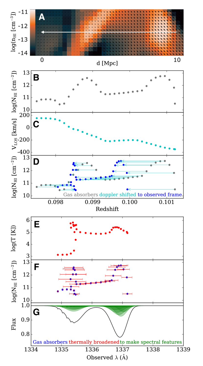
Figure 5 illustrates the process by which the SpectrumGenerator produces a Lyman-$\alpha$ absorption feature from a sightline passing through a low-resolution simulation volume. This figure clearly depicts how physical structures can be traced directly to features in the final spectrum based on density, temperature, and velocity data.

The resulting spectrum can subsequently be post-processed to make it resemble realistic telescopic data (see Section 2.5), or it can be saved to disk as is. trident supports saving spectra as tab-delimited text files, as hdf5 files, or as fits files. trident also contains a sophisticated plotting routine built on top of matplotlib (Hunter, 2007) for plotting the spectrum in various ways quickly and easily.

2.4.1 Voigt profile calculation

A spectral absorption line is caused by an atom or ion absorbing incident light of a particular energy in order to boost itself to a higher quantum energy state. In an ideal environment with a single particle, the result is an absorption line consisting of a perfect delta function at the wavelength corresponding to the energy of the difference between the particle’s quantum states. However, in practice there are a number of processes that broaden this delta function based on the characteristics of the gas. The two most important processes are doppler broadening, due to the velocity distribution of the gas particles, and pressure broadening, caused by the collisions of the gas particles against each other. Doppler broadening is well-described by a Gaussian function, whereas pressure broadening can be modeled with a Lorentzian function. The convolution of these two functions is called the Voigt profile, and it is commonly used to model spectral line profiles, yielding a value for the optical depth $\tau$ at different wavelengths. For reference, Section 4.2 demonstrates the Voigt Profile shape at various spectral line strengths.

The Voigt Profile in trident is calculated consistent with the method described in Hill (2016) reproduced in part here. The Voigt Profile $V(x,\sigma,\gamma)$ is the convolution of the Gaussian Profile $G(x,\sigma)$ and the Lorentzian Profile $L(x,\gamma)$, where $x=\nu-\nu_{0}$, the range of frequencies relative to the line center frequency, $\sigma$ is the standard deviation of the Gaussian, and $\gamma$ is the half-width half-max of the Lorentzian:

$$G(x,\sigma)=\frac{1}{\sigma\sqrt{2\pi}}\exp\left(\frac{-x^{2}}{2\sigma^{2}}\right)$$ (13)

$$L(x,\gamma)=\frac{\gamma/\pi}{x^{2}+\gamma^{2}}$$ (14)

$$V(x,\sigma,\gamma)=\int_{-\infty}^{\infty}{G(x^{\prime},\sigma)L(x-x^{\prime},\gamma)d\lambda^{\prime}}$$ (15)

Let us adopt $\lambda$ as our independent variable instead of $x$, since trident operates in wavelength space. The Voigt Profile possesses no closed form, but it can be numerically calculated as:

$$V(\lambda,\sigma,\gamma)=\frac{\Re[w(z)]}{\sigma\sqrt{2\pi}}\textrm{, where }z=\frac{u+ia}{\sigma\sqrt{2}}$$ (16)

and $w(z)$ is the Faddeeva function, a scaled complex complementary error function (Poppe & Wijers, 1990), defined as:

$$w(z)=\exp{(-z^{2})}\left(1+\frac{2i}{\sqrt{\pi}}\int_{0}^{z}{e^{t^{2}}}dt\right)$$ (17)

The complex components of $z$ consist of $u$, our range of wavelengths relative to line center, and our damping parameter $a$:

$$u=c\left(\frac{\lambda_{0}}{\lambda}-1\right)\textrm{ and }a=\frac{\Gamma\lambda_{0}}{4\pi}$$ (18)

where $c$ is the speed of light, $\lambda_{0}$ is the central wavelength of the Voigt Profile, and $\Gamma$ is the sum of the transition probabilities (i.e., Einstein A coefficients) for the ionic transition.

This optical depth, $\tau$, for a line is calculated by scaling the resulting Voigt Profile by the peak optical depth $\tau_{0}$ at the spectral line’s center (Armstrong, 1967):

$$\tau(\lambda,\sigma,\gamma)=\tau_{0}V(\lambda,\sigma,\gamma)$$ (19)

$$\tau_{0}=\frac{\pi e^{2}Nf_{val}\lambda_{0}}{m_{e}c}$$ (20)

where $e$ and $m_{e}$ are the charge and mass of the electron, $c$ is the speed of light, $N$ is the absorber’s column density, and $f_{val}$ is the oscillator strength of the ionic transition.

Figure 6.— Subgrid deposition method. When absorption features are narrower than the spectral bin width, trident creates an array of virtual bins at higher spectral resolution to assure flux conservation of unresolved features. Top: Depositing a narrow Lyman-$\alpha$ feature (dashed blue line) into a spectrum with coarse 1 angstrom spectral bins $w_{line}<w_{bin}$). Middle: trident creates an array of virtual bins with 0.1 angstrom resolution (green bins) into which we deposit the Voigt profile to approximate the line’s flux deficit. Bottom: We numerically integrate the area of the virtual bins to calculate the equivalent width of the unresolved spectral line on our original coarse bins (grey bins).

2.4.2 Voigt profile deposition

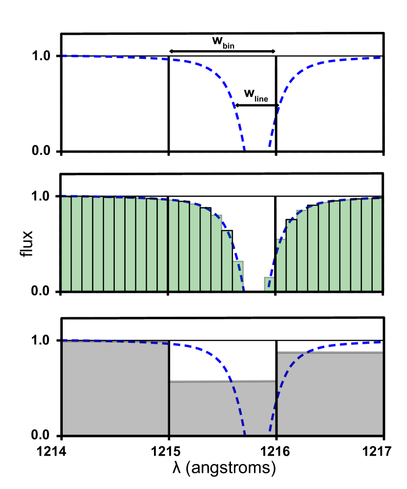
Each time a spectral feature is added, trident identifies the wavelength bin where its deposition will be centered. However, because there is no closed form for the Voigt Profile, it is difficult to know a priori how wide a spectral absorption feature will extend in wavelength space. Therefore, trident adaptively increases the size of the window over which it deposits the spectral feature, sampling the Voigt Profile at the center of each bin location in the spectral window. trident repeats this operation until the window is wide enough that the deposited $\tau$ values at the edges of the window are less than $10^{-3}$ before depositing the entire Voigt Profile into the spectrum.

On the other hand, spectral features that are too small, narrower than the chosen wavelength bin width, would be ignored by the algorithm and lost since the SpectrumGenerator only calculates the Voigt Profile at the centers of each wavelength bin. Ignoring these narrow features leads to the total $\tau$ and flux being dependent on the chosen wavelength bin width, which is inherently unphysical.

To address this problem, trident performs subgrid deposition when it recognizes that the thermal width of a spectral line is narrower than the spectral bin width in SpectrumGenerator. Subgrid deposition creates an array of virtual spectral bins, each less than one tenth the thermal width of the spectral feature. trident deposits the Voigt Profile to these virtual bins, then numerically integrates them to determine the equivalent width of the spectral line at the original low-resolution wavelength bin. This process conserves $\tau$ and total flux regardless of the wavelength bin width used in the output spectrum. The process of subgrid deposition is illustrated in Figure 6.

Figure 7.— From bottom to top, we show the progression of an increasingly complex synthetic absorption spectrum from a clean, raw spectrum to one with all of the components described in Section 2.5. The spectral components are added in the following order: Composite quasar spectrum (QSO), Milky Way foreground (MW), line spread function (LSF), noise. The left panel shows the entirety of the generated spectrum while the right panel shows a zoomed in region of the spectrum to allow one to see the significance of the post-processed modifications of the original spectrum. The light ray used for this spectrum comes from a 1536³ cosmological enzo dataset aimed at probing the nature of the intergalactic medium and traverses a range in redshift from $z=0.0$ to $z=0.03295$. It includes a set of common UV spectral lines.

2.5. Post-processing the spectrum

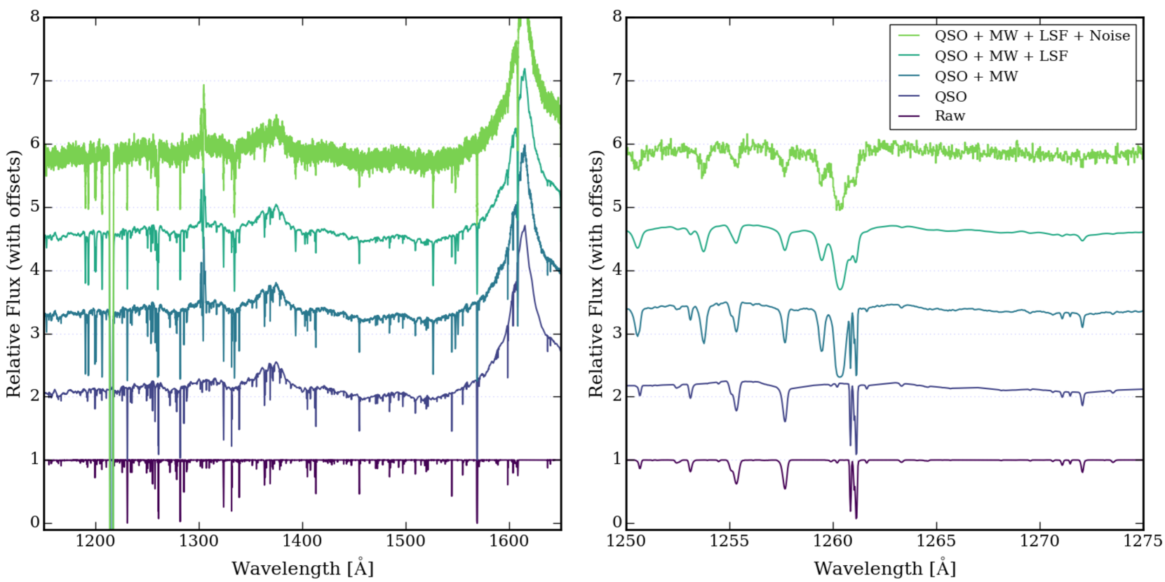
Once a “raw” spectrum has been generated, additional levels of complexity can be added by trident. These additional features are intended to produce progressively more realistic synthetic spectra that can be directly compared to observational datasets using the same analysis tools employed by observers. Figure 7 illustrates how trident can post-process a raw spectrum to make it more realistic according to the steps below.

First, in order to make comparisons with observational quasar sightlines, the most basic spectrum modification includes the addition of an underlying quasar spectrum at a desired redshift, usually the far redshift $z_{a}$ of the LightRay. This is accomplished by taking the composite QSO spectrum calculated by Telfer et al. (2002), shifting it to the desired redshift, and computing an interpolated relative flux as a function of wavelength. This interpolated and shifted spectra is then multiplied by the raw spectrum to add the effects of the background quasar. To further approach realism with our synthetic spectrum, we can also introduce spectral features due to foreground contamination from the Milky Way (MW). Similar to the method introduced for adding a background QSO spectrum, instead we use the average MW foreground computed by Danforth et al. (2016).

Once a spectrum is produced that contains all of the desired observational signatures, one can further modify the spectrum by applying a set of instrument-specific properties, as suggested in Section 2.4. First, to most accurately match the desired instrument, the initial spectrum uses the known pixel resolution of the instrument for the wavelength bin size then, in this post-processing step, the spectrum is convolved with the line spread function (LSF) of the specified instrument. trident can currently convolve TopHat and Gaussian kernels with its spectra, and it additionally accepts custom kernels. In the case of mimicking the Cosmic Origins Spectrograph, we convolve the spectrum with an average LSF computed for each observing mode’s kernel. Furthermore, trident readily allows for the addition of other instrument properties through its built-in Instrument class.

Finally, we allow for the addition of Gaussian random noise. For a specified value of the signal-to-noise ratio (SNR), random fluctuations drawn from a Gaussian distribution are added to the spectrum. Alternatively, an arbitrary noise vector can be supplied by the user. The resulting spectrum is as realistic as possible.

3. Demonstration: how to run trident

Here we provide an annotated example Python script for a common use-case of trident. This script generates a COS spectrum of a sightline passing through the center of an art-ii dataset. This script and others that are similar can be found in our documentation to step you through the process with different simulation codes.

First, we load the relevant Python modules of yt and trident. We set the dataset filename and load the dataset into yt. The dataset used is the publicly available initial output of an art-ii run of an isolated galaxy used in an agora paper (Kim et al., 2016) assumed to be at redshift of 0. We define the trajectory of our LightRay sightline to cross the full domain of our simulation, and additionally define what lines, ions, or atoms we want to include in our spectrum. trident is extremely flexible in terms of what lines we can include. Here we will include all lines produced by all ions from hydrogen and silicon, singly-ionized magnesium (Mg II), and the 1335 $\rm\AA$ line from singly-ionized carbon (C II).

import yt
import trident as tri
fn = ‘AGORA_LOW_000000.art’
ds = yt.load(fn)
ray_start = ds.domain_left_edge
ray_end = ds.domain_right_edge
line_list = [‘H’, ‘Si’, ‘Mg II’, ‘C II 1335’]

Now, we create a sightline through the dataset, using the trajectory and field requirements we defined. We will save it to disk as ray.h5 as well as use it locally. Note that we have set our ftype keyword to ‘gas’. This is the yt-based field type indicating where trident should do the ion_balance calculations. Here we set it to ‘gas’ because this is an art-ii dataset and AMR codes should make the ion interpolations on the grid, denoted by ‘gas’. However, for SPH datasets, the interpolation must occur on the particle itself before being smoothed to the grid. Thus one would set ftype to be the field type associated with the frontend’s gas particles (e.g. PartType0 for gadget and gizmo, Gas for gasoline, etc.).

ray = tri.make_simple_ray(
                ds,
                start_position=ray_start,
                end_position=ray_end,
                lines=line_list,
                ftype=‘gas’)

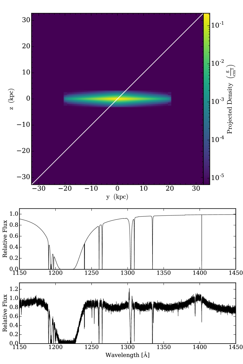
We can then take a look at the path of our sightline through the simulated volume by using yt’s functionality to create an image of our simulated volume down the $x$-axis in projected gas density, zoom in on the center, overplot the path of the ray on our projection, and save it to disk.

p = yt.ProjectionPlot(ds, ‘x’, ‘density’)
p.annotate_ray(ray)
p.zoom(20)
p.save(‘projection.png’)

From this LightRay object we just created, we will generate an absorption spectrum using the defaults associated with the Cosmic Origins Spectrograph instrument aboard the Hubble Space Telescope. This sets things according to the G130M observing mode where the spectral range is 1150-1450 Å, the spectral bin size is 0.01 Å, and the appropriate line spread function is applied. The user could easily define their own instrument with arbitrary settings. This raw spectrum is now saved to a tab-delimited text file, and the spectrum is plotted to an image.

sg = tri.SpectrumGenerator(‘COS’)
sg.make_spectrum(ray, lines=line_list)
sg.save_spectrum(‘spec_raw.txt’)
sg.plot_spectrum(‘spec_raw.png’)

Lastly, we do some post-processing to the resulting spectrum, adding in a background quasar, and the Milky Way foreground, applying the defined line spread function to it, and adding gaussian noise with a signal-to-noise ratio of 30. These steps are performed to make our data as much like spectra an observer would obtain through a real spectrograph. We then plot and save the “final” spectrum.

sg.add_qso_spectrum()
sg.add_milky_way_foreground()
sg.apply_lsf()
sg.add_gaussian_noise(30)
sg.plot_spectrum(‘spec_final.png’, step=True)

Figure 8 displays the three images that are generated by this working script, showing the path of the LightRay sightline as it probes the isolated disk galaxy, the raw spectrum, and the post-processed COS-like spectrum. While this dataset and script are extremely simple, we are able to reproduce the spectrum of a damped Lyman-$\alpha$ absorber with several accompanying lines including some silicon and oxygen lines. Because this script and dataset are freely available, we encourage readers to reproduce this result on their own.

Figure 8.— Resulting images from our annotated demonstration. Top: Density projection of isolated galaxy simulation taken from agora team showing path of LightRay. Middle: Raw spectrum of our LightRay featuring lines from H, Si, Mg II, and the C II 1335 Å line. Bottom: Final post-processed spectrum also including quasar background, milky way foreground, COS line-spread function, and signal to noise of 30.

4. Discussion

4.1. Comparison with real spectra

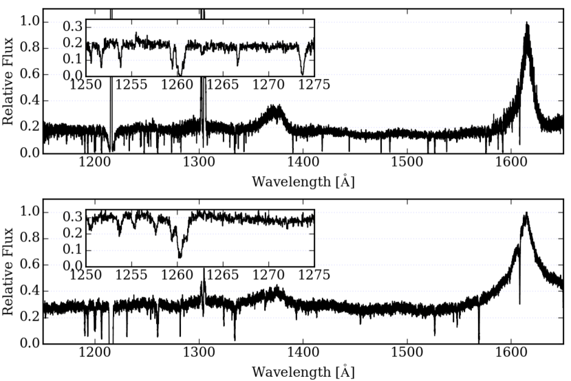
We can assess how well trident creates synthetic spectra by making a direct comparison against equivalent observational data. IGM LightRays are generally compound rays, sightlines that pass through several simulation outputs to create a long enough trajectory to reach high redshift sources. Figure 9 compares a publicly-available QSO spectra from Danforth et al. (2016) to a synthetic spectrum from outputs of simulation similar to those of Smith et al. (2011). For the purposes of this comparison, the synthetic spectrum is generated using the instrument properties of COS to match the observational characteristics of the true spectrum. As can be seen, the spectra are similar in shape, in the location of major features, and in the locations of many spectral lines. Subsequent analysis can be performed using automated Voigt profile fitting algorithms (e.g. Davé et al., 1997; Egan et al., 2014) to extract the “observed” properties of the the simulated IGM. Taken a step further, trident-generated spectra like the one in Figure 9, readily enable the creation of community tools like the MAST Interface to Synthetic Telescopes with yt (MISTY; Peeples, 2014), a public simulation-to-archive pipeline that simplifies the process of accessing and interacting with synthetic spectra.

Figure 9.— Top: COS Spectrum for a QSO at z=0.3295 from data made available by Danforth et al. (2016) Bottom: trident synthetic spectrum for a QSO at z=0.3295 using a light ray from an 1536³ cosmological enzo dataset similar to those presented in Smith et al. (2011). Both of the inset plots show the same zoomed-in region of wavelength space for each spectrum.

4.2. Code test: curve of growth

Due to the extreme conditions found in the low-density astrophysical environments probed by absorption-line spectra, it is very challenging to make explicit tests to assure that trident exactly reproduces the spectra from experimental data. However, one viable test is to demonstrate how well trident reproduces the so-called curve of growth, the relationship between the an ion’s column density and its resulting absorption strength. The curve of growth is a well-studied problem with a clear empirical-derived physical solution relating the equivalent width $W$ of a spectral absorption line to the number density $N$ of that ion along the probed sightline.

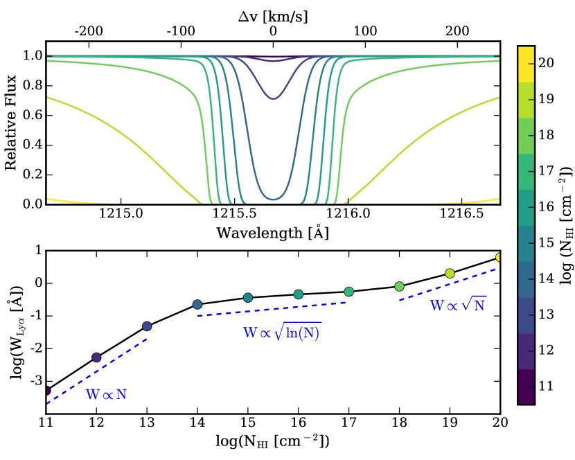
As described in Section 2.4.1, absorption line shapes follow a Voigt Profile, a combination of the relatively narrow Gaussian profile with the relatively wide Lorentzian profile. The complex shape of the Voigt profile leads to a non-linear relationship between the column density of an absorber and its corresponding spectral line strength. Observers commonly use the equivalent width of a spectral line $W=\int{(1-f_{\lambda}/f_{0})d\lambda}$ as a proxy for its strength. In Figure 10, we have plotted several Lyman-$\alpha$ absorption features deposited at various neutral hydrogen column densities at a doppler parameter of 22 km s^-1 on top, and the resulting curve of growth indicating their corresponding equivalent widths on bottom.

In the optically thin limit, when an absorption line does not block out all of the flux at a given wavelength, it is said to be in the “weak” or “linear” regime of the curve of growth. The Voigt Profile approximates a gaussian, where increases in column density cause proportional increases in the equivalent width of the absorption line. The first three shallow absorption features ($N_{\rm HI}=10^{11}-10^{13}$ cm^-2) all sit within the “linear” regime of the curve of growth where $W\propto N$.

As the absorption features increase in strength and become opaque enough to saturate and block out all flux at a given wavelength, increases in column density are met with negligible increases in the line’s equivalent width. Because the Voigt Profile is still dominated by the Gaussian Profile, increases in column density do little to increase the depth of the line. This regime is termed “flat” or “saturated”, and it shows up in Figure 10 as the middle four absorption features ($N_{\rm HI}=10^{14}-10^{17}$ cm^-2) where $W\propto\sqrt{\ln{N}}$.

Finally, very strong lines start to behave more like a Lorentzian Profile, where the wings block increasing amounts of flux in surrounding wavelengths. This regime is referred to as “strong” or “damped”. The growth of the equivalent width is slow in this regime, and only increases with the square root of the column density. The “damped” lines are the three strongest lines in Figure 10 for absorption features ($N_{\rm HI}=10^{18}-10^{20}$ cm^-2) where $W\propto\sqrt{N}$.

The behavior of the curve of growth in trident perfectly reproduces the textbook case, thereby validating these aspects of trident’s operation.

Figure 10.— Top: Voigt profiles of the Lyman-$\alpha$ line for different neutral hydrogen column densities at $T=30,000$ K ($b=22$ km s^-1) as produced by trident. Bottom: Corresponding curve of growth describing the relationship between each line’s column density and line equivalent width. Dashed lines indicate the linear (left), saturated (center), and logarithmic (right) portions of the curve of growth as reproduced by trident.

4.3. Limitations of trident and its data tables

4.3.1 Limitations of trident

While the availability of a code like trident is a benefit to the astrophysical community, it has several limitations that should be noted when using it and interpreting its results for scientific research. Many of the limitations listed below can be addressed in future versions of the code or by including more detail in the underlying simulations themselves before using trident.

trident does not perform full radiative transfer on the simulation. A radiative transfer (RT) code approximates how electromagnetic waves propagate between all of the emitters and absorbers in a simulated volume over various wavelength photons. RT codes can produce very realistic photometry, spectroscopy, and IFU data, but they are computationally expensive to run at comparable resolution to observational data, and oftentimes they lack relevant physics (e.g. line transfer). trident only tracks the absorption effects along the desired sightline, but it is fast and possesses a number of additional features missing from most RT codes making it a good complement to RT analyses.

SPH codes deposit ion fields to a grid before sightline integration. Because trident operates as an extension of yt, it inherits yt’s treatment of particle-based codes. At present, yt converts particle-based codes outputs into a grid-based format in order to leverage yt’s extensive framework for processing and analyzing grid data. The process is performed conservatively, depositing the particles to an adaptive grid using a scatter operation at the cell centers to preserve the inherent dynamic resolution of the dataset and utilize the unique smoothing kernel of the original simulation code for the deposition. Furthermore, the ionic abundance calculations of ion_balance (see Section 2.2) take place on the particles themselves prior to their deposition to the grid. Most particle-based absorption-line synthetic spectral generators (e.g. Oppenheimer & Davé, 2006) calculate a sightline’s column density by directly integrating its trajectory through the smoothing kernel of each intersected SPH particle. Preliminary analysis indicates agreement between this traditional SPH integration method and the grid-based method adopted by trident to $<\sim 10$% (Dong et al., in prep). Therefore, the grid-based treatment of SPH particles is not a limitation per se, but it requires explanation. The next version of trident, expected out by end of 2017, will incorporate particle kernel direct integration consistent with other particle-based spectral generation codes.

4.3.2 Limitations of the current ion_balance data tables

It is impossible to calculate the exact abundance of a given ion by simply knowing the instantaneous gas density, temperature, and metallicity fields, but trident does a fair job at estimating it. However, there are several assumptions built into the currently available data tables used by the ion_balance module to approximate ionic species abundances. Recall that ion_balance operates by plugging a gas parcel’s density, temperature, and radiation field (vis-a-vis redshift) into a three-dimensional data table to interpolate and determine the relative abundance of its desired ionic species. The lookup table is populated by thousands of individual cloudy runs varied over these gas densities, temperatures, and radiation fields. For a full description of how ion_balance operates, see Section 2.2 and Appendix C.

trident provides a few data tables assuming different UV background models (Haardt & Madau, 2012; Faucher-Giguère et al., 2009), but at present these suffer from some limitations. These limitations can be avoided by simulating and tracking the ionic species in your hydrodynamical simulation that you wish to use in the generation of synthetic spectra and avoiding use of the ion_balance module entirely. Furthermore, users can generate their own data tables with publicly available code (Smith et al., 2008). However, take heed of the following limitations based on the assumptions inherent in the default lookup tables when using ion_balance to approximate ionic abundances.

Current ion_balance data tables assume UV background radiation operates in the optically thin limit. At present, the data tables provided to ion_balance were produced by including the full effect of the UV background, ignoring any self-shielding effects of gas deeply embedded in a high-opacity envelope. Gas with neutral hydrogen columns $N_{HI}<10^{17.2}$ cm^-2 shield nearby gas from ionizing radiation E $<$ 13.6 eV (Faucher-Giguère & Kereš, 2011). This effect has been approximated in previous work (Rahmati et al., 2013), and the next version of trident, due out by the end of 2017, will account for it. Currently ignoring the effects of self-shielding will artificially raise the ionization state of the various low ions present to some degree, particularly in clumped regions.

Current ion_balance data tables ignore local photo-ionizing sources. Currently, the strength and the spectrum of the UV background radiation field used to generate the lookup tables does not account for additional local sources of ionizing radiation which may be present in the simulation, like AGN and massive stars. This is a common approach used by other groups, since including additional radiation source terms (and additional dimensions) in the ion_balance data table would make it extremely large. Notably, Shen et al. (2013) calculated that local photo-ionizing effects from an L* galaxy with a galactocentric star formation rate of SFR = $20M_{o}/yr$ were only dominant over the metagalactic UV radiation field within 45 kpc of the galactic center. Therefore, by not accounting for local photoionizing sources in the data tables, ion_balance artificially reduces the ionization state of gas in the interiors of AGN and starburst galaxies.

ion_balance data tables assume ionization equilibrium. In the absence of fields in the original simulation that explicitly follow the evolution of a desired ionic species, it is impossible to calculate its non-equilibrium state instantaneously. Thus, ion_balance estimates an ion’s abundance by using the aforementioned photoionization from a UV background coupled with collisional ionization. Ionization equilibrium remains valid in high-density, low-temperature regime where the cooling time is short, but it breaks down in the low-density parts of the IGM (Cen & Fang, 2006). Studies suggest that ionization fractions can vary between equilibrium and non-equilibrium treatment of high ionization species of oxygen gas in the CGM and IGM at the $\lesssim 30$% level (Cen & Fang, 2006, Oppenheimer et al., 2016, Silvia et al, in prep). In these studies, the equilibrium models predict a reduced ionization state of gas for high ions in low-density environments.

5. Summary

In this paper, we have presented trident, a parallel, Python-based, open-source code for producing synthetic observations from astrophysical hydrodynamical simulation outputs. Its features include:

• post-processing simulation outputs to include ion density fields for any desired ion based on instantaneous fluid and ionizing radiation conditions

• creating LightRays, ordered one-dimensional arrays sampling the fields in a dataset along a chosen sightline or across multiple consecutive simulation outputs to approximate a sightline spanning a large redshift interval;

• generating a spectrum from the fluid quantities contained in a LightRay object and a custom list of relevant ions and spectral lines;

• post-processing a spectrum to match the characteristics of a spectrum observed by a real spectrograph including its wavelength range, spectral resolution, line spread function, noise, etc.;

• full support for simulations for all major astrophysical hydrodynamical code formats;

• automatic parallelization for both sightline and spectral generation using mpi;

• ability to directly trace physical structures to their resulting spectral features and vice versa (see Figure 5);

We encourage members of the scientific community to both use and contribute to trident. For more information on acquiring, installing, and using trident, please see Table 1.

6. Acknowledgements

We are extremely grateful to our co-developers within the yt community for their assistance in coding, reviewing, testing, and timing releases of yt to match the trident development schedule. In particular, we wish to thank Matthew Turk, Nathan Goldbaum, Kacper Kowalik, and John ZuHone for going above and beyond the requirements of a open-source software community. Special thanks go out to Bili Dong, Lauren Corlies, and Andrew Emerick for early code contributions. trident benefited greatly from our discussions with the aforementioned and also Molly Peeples, Brian O’Shea, X Prochaska, Nicolas Tejos, Jess Werk, Jason Tumlinson, Nick Earl, Kate Rubin, Nicholas Lehner, Josh Peek, Chuck Steidel, Gwen Rudie, Sean Johnson, Ben Oppenheimer, Amanda Ford, Romeel Dave, Robert Thompson, David Weinberg, Neal Katz, Joel Primack, Ian McGreer, Greg Bryan, Phil Hopkins, Paul Torrey, Josh Suresh, Simeon Bird, Dus̆an Keres̆, Claude-André Faucher-Giguère, Erika Hamden, and Clayton Strawn. We are especially grateful to Charles Danforth and Ian McGreer for the quasar and Milky Way templates they provided. We thank Jacob Kneibel for his work on the early stages of generating realistic synthetic spectra, particularly in using COS LSFs. Also thanks goes to Ji-hoon Kim and members of the agora consortium for providing datasets to test trident across many simulation formats. Support for this work was provided by NASA through Hubble Space Telescope Theory Grants HST-AR-13917, HST-AR-13919, HST-AR-13261.01-A and HST-AR-14315.001-A and ATP grants NNX09AD80G and NNX12AC98G from the Space Telescope Science Institute, operated by the Association of Universities for Research in Astronomy, Inc., under NASA contract NAS 5-26555. Additional support comes from the NSF through AST grant 0908819 and the NSF Astronomy and Astrophysics Postdoctoral Fellowship program. Computational resources for this work were provided through NSF XSEDE grant TG-AST140018, NSF BlueWaters grants PRAC-gka and GLCPC_jth. This research also used resources of the National Energy Research Scientific Computing Center (NERSC), a DOE Office of Science User Facility supported by the Office of Science of the U.S. Department of Energy under Contract No. DE-AC02-05CH11231. We acknowledge access to NERSC resources made possible by University of California High-Performance AstroComputing Center (UC-HiPACC).

Software

hdf, h5py, scipy, numpy (van der Walt et al., 2011), matplotlib (Hunter, 2007), mpi (Forum, 1994), mpi4py (Dalcin et al., 2005), yt (Turk et al., 2011), and astropy (Astropy Collaboration et al., 2013).

Appendix A Parallelism and Performance

The two primary classes of trident, LightRay and SpectrumGenerator, are both parallelized using mpi. This is implemented using the parallel_objects helper function from yt, which is itself built upon the mpi4py module. The parallel_objects function is a loop iterator that divides iterations between mpi work groups and facilitates the re-joining of results from all groups at the end of the loop. Use of parallelism in both yt and trident scripts requires that yt.enable_parallelism() be present after module imports.

The LightRay creation step is parallelized by splitting up the simulation datasets required for compound ray generation over the available mpi processes, typically in single-process work groups. In the case where there are more available processes than datasets (such as for simple rays), multiple processes can be allocated to an instance of a single dataset, making use of yt’s internal parallelism to partition the work.

The SpectrumGenerator is parallelized using a similar, two-layered approach. First, the generation of a single spectrum is parallelized over the absorption lines to be deposited (i.e., Ly-$\alpha$, Ly-$\beta$, etc.). If the number of available processes exceeds the number of lines to be deposited, then the line deposition task itself is split among available processes for depositing each absorber. In the limit where the number of lines and/or absorbers is much greater than the number of available processes, this parallelism strategy scales well and is, in practice, limited by the speed and parallelism of the filesystem. In addition, the yt parallel_objects function can be used directly by the user for the embarrassingly parallel task of operating over multiple LightRay objects and their subsequent spectra.

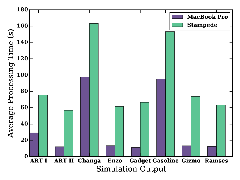
As a reference benchmark, we ran trident on the agora idealized galaxy simulations (Kim et al., 2016). We ran the script provided in Section 3 (without the ProjectionPlot step) on the initial outputs for each of the simulations codes supported in the agora study. These scripts were run on two machines: (1) an early 2015 MacBook Pro with 3.1 GHz Intel Core i7 processor and 16 GB RAM, and (2) a single Intel Xeon E5 Sandy Bridge processor on Stampede, the National Science Foundation’s flagship supercomputing cluster run by the Texas Advanced Computing Center (TACC) as part of the Extreme Science and Engineering Discovery Environment (XSEDE) initiative. The script was modified slightly to send ten sightlines through the central galaxy and create a spectrum for each. Figure 11 shows the average amount of time trident takes to generate a single sightline and spectrum. Stampede compute cores are substantially slower than the MacBook Pro presumably due to file system load. The increased processing time required for gasoline and changa particle-based codes reflects the particle deposition step described in Section 2.2 and the fact that fields are not cached between sightline generation. As previously noted in Section 4.3.1, the next trident release will address these issues affecting particle-based code performance by numerically integrating particle kernels on the fly and avoiding the particle deposition step altogether.

Figure 11.— Average trident processing time to generate a simple ray and spectrum for different simulation outputs from the agora isolated galaxy simulations (Kim et al., 2016).

Subsequent profiling of this benchmark script reveals that $\sim 60\%$ of the processing time is taken by the SpectrumGenerator, made up of equal parts voigt profile calculation, subgrid deposition, and array bookkeeping. Creation of the LightRay requires about $\sim 20\%$ of the processing time primarily spent calculating what cells are intersected by the sightline and then accessing and saving these data. The remaining time spent is miscellaneous time associated with applying the line spread function, saving the LightRay and spectra to disk and figures, etc. Notably, less than 1% of the run time is spent in the ion_balance portion of trident.

Appendix B Accuracy of ion_balance tables

The dependency of a given ionization state of gas is a very complex and non-linear function of its gas density, temperature, and incident radiation field. As described in Section 2.2, trident approximates this dependency by interpolating over a large three-dimensional look up table created by thousands of one-cell cloudy models (Ferland et al., 2013). However, the resolution of this data table will determine how well this non-linear three-dimensional function can be sampled to provide adequate estimates of ionic abundances.

We estimate the level of error for a data table by taking the sum of all ionization fractions for a given species over a grid of random points that span the density/temperature/redshift parameter-space of the data table. In reality, all ionization fractions species for a given species should always add to 1 (e.g. $f(\rm H_{\rm I})+f(H_{II})=1.0$). We measure how much the sum of our ionization fractions for a species deviate from 1 as an estimate of the error of the data table.

We perform this test using low and high resolution data tables for the Haardt & Madau (2012) UV background model used by trident and available for download. The high-resolution table (296 MB) is the default that we recommend for users, but the low-resolution table (41 MB) is provided for users concerned about disk space or bandwidth. Both data tables span their density, temperature, and redshift dimensions as: -9 $\leq$ log($n_{\rm H}$ / cm^-3) $\leq$ 4; 1 $\leq$ log(T / K) $\leq$ 9; and 1 $\leq$ log(1 + z) $\leq$ 1.2. The low resolution table samples the density, temperature, and redshift dimensions with 27, 161, and 22 points, respectively. The high resolution table samples the density, temperature, and redshift dimensions with 105, 321, and 22 points, respectively, and is thus 8 times larger than the low resolution table. We find the error to be significantly dependent on redshift, so we use the same set of random densities and temperatures within each redshift bin covered by the input table.

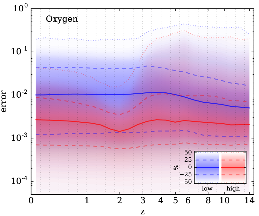
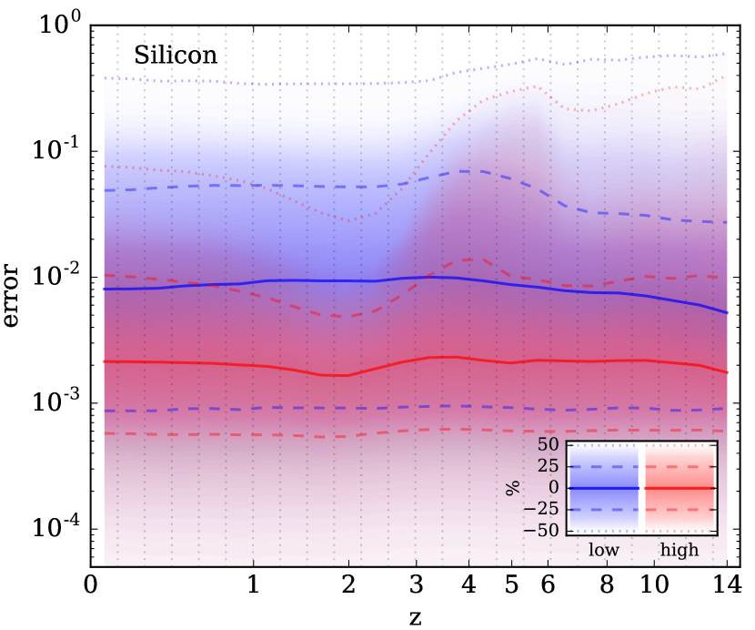
In Figures 12 and 13, we show the distribution of error in ionization fraction for O and Si. In each case, we use 100,000 random points in log($n_{\rm H}$ / cm^-3) and log(T / K) for each redshift bin. For each redshift bin, we select random redshifts within the bin. We define the error as

$$error=1-\sum_{i=1}^{N}f_{i},$$ (B1)

where $f_{i}$ is the ionization fraction of the i’th species of any element with N total ionization states. We find that the total ionization fraction only ever exceeds 1 by maximally $\sim 10^{-3}$, and so we only show situations where the total ionization fraction is less than 1. For both O and Si, the average error is about 1% for the low resolution table and about 0.2% for the high resolution table. We find rare cases where the error can be significantly larger. For oxygen, the error can reach $\sim$40/32% in the low/high resolution tables at redshifts $z\sim$ 5.5. This is even higher for silicon, due mainly to the greater number of ionization states. However, at redshifts less than 2, the maximal error for the high resolution table never exceeds 5% for O and 8% for Si.

While interpolation over the data table works well, extrapolation beyond its bounds can create some problems. trident does not explicitly support data with densities or temperatures outside the range provided above. If an extrapolation yields an unphysical ionization fraction for an ion, for instance one greater than one, trident will cap it at one and warn the user. This can occur for calculating ionization fractions of low ions at exceptionally cold temperatures outside our provided temperature ranges (e.g. 1 K).

Figure 12.— Levels of error in oxygen ionization fraction calculations by ion_balance when using the Haardt-Madau data tables. Error is defined in Appendix B. Blue shaded regions show the error distribution for the low resolution table, and red shaded regions show the high resolution table. The solid lines show the median error, dashed lines show $\pm$25%, and the dotted line shows the maximum error. The horizontal, grey dotted lines show the redshift bins of the input data.

Figure 13.— Same as Figure 12, but for Silicon.

Appendix C Ion density generation

Here we describe the full algorithm that trident employs in the ion_balance module to generate the number density field for a desired ionic species. The ionic number density field can be derived in different ways depending on the fields that exist in the simulation output dataset. In short, for a desired ion field (e.g. O VI), trident will use the on-disk field if present in the simulation, otherwise trident employs ion_balance on the appropriate metal field when present (e.g. oxygen abundance), or in the case that the desired metal fields are not tracked at all, trident assumes a solar abundance of the desired metal from the bulk metallicity field (e.g. $Z$). Solar abundance values are extracted from the documentation of Cloudy (Ferland et al., 1998) based on previous work (Grevesse & Sauval, 1998; Holweger, 2001; Allende Prieto et al., 2001, 2002). Hereafter describes the full algorithm for the curious reader:

Define $X_{i}$ as the $i$’th ion of element $X$. The total number density of $X_{i}$ is

$$n_{X_{i}}=f_{i}\ n_{X},$$ (C1)

where

$$f_{i}\equiv\frac{n_{X_{i}}}{n_{X}},$$ (C2)

and $n_{X}$ is the total nuclei number density of all species of $X$. In terms of the mass density, $\rho_{X}$,

$$\rho_{X}=n_{X}\ m_{X},$$ (C3)

where we define the atomic mass of $X$, $M_{X}$, as

$$m_{X}\equiv M_{X}\ m_{H},$$ (C4)

and $m_{H}$ is the Hydrogen mass.

The goal is to generate $n_{X_{i}}$, but different base fields will exist, depending on the dataset. If $\rho_{X}$ exists, then

$$n_{X}=\frac{\rho_{X}}{M_{X}\ m_{H}}$$ (C5)

and

$$n_{X_{i}}=\frac{f_{i}\ \rho_{X}}{M_{X}\ m_{H}}.$$ (C6)

If $\rho_{X}$ does not exist, then there are two possibilities. First, we define the solar abundance of element $X$, $A_{X}$, as

$$A_{X}=\frac{n_{X}}{n_{H}}|_{\odot}.$$ (C7)

$X$ is either H or He.

$$n_{X}=A_{X}\ n_{H}.$$ (C8)

If we have $\rho_{H}$, then we can say

$$n_{X}=A_{X}\ \frac{\rho_{H}}{m_{H}}.$$ (C9)

If we do not have $\rho_{H}$, then we will assume the primordial H mass fraction, $\chi=0.76$. In that case, we have

$$n_{H}=\frac{\chi\ \rho}{m_{H}}$$ (C10)

and

$$n_{X}=A_{X}\ \frac{\chi\ \rho}{m_{H}}.$$ (C11)

If $X$ is a metal, then define the metallicity of $X$ as

$$Z_{X}=\frac{\rho_{X}}{\rho}.$$ (C12)

If we have $Z_{X}$ and equation C5, then

$$n_{X}=\frac{Z_{X}\ \rho}{m_{H}\ M_{X}}.$$ (C13)

If we do not have $Z_{X}$, then we must use the solar abundance and the total metallicity, $Z$, given by

$$Z=\frac{\rho_{metals}}{\rho},$$ (C14)

and

$$\rho_{X}=Z\ \rho\ \frac{\rho_{X}}{\rho}|_{\odot}$$ (C15)

Taking $\rho_{X}$ and $\rho_{H}$, we have

$$\frac{\rho_{X}}{\rho_{H}}=\frac{n_{X}\ M_{X}\ m_{H}}{n_{H}\ m_{H}}.$$ (C16)

Canceling out the $m_{H}$, we have

$$\frac{\rho_{X}}{\rho_{H}}=\frac{n_{X}\ M_{X}}{n_{H}},$$ (C17)

and

$$\frac{\rho_{X}}{\rho_{H}}|_{\odot}=\frac{n_{X}}{n_{H}}|_{\odot}\ M_{X},$$ (C18)

and with equation C7, we get

$$\frac{\rho_{X}}{\rho_{H}}|_{\odot}=A_{X}\ M_{X}.$$ (C19)

Equation C15 then becomes

$$\rho_{X}=Z\ \rho_{H}\ A_{X}\ M_{X}.$$ (C20)

Finally, if we don’t have $\rho_{H}$, we use $\chi$ to get

$$\rho_{X}=Z\ \chi\ \rho\ A_{X}\ M_{X}.$$ (C21)

This gives us

$$n_{X}=\frac{Z\chi\ \rho\ A_{X}}{m_{H}}$$ (C22)

and

$$n_{X_{i}}=\frac{f_{i}Z\chi\ \rho\ A_{X}}{m_{H}}.$$ (C23)

References

- Allende Prieto et al. (2001) Allende Prieto, C., Lambert, D. L., & Asplund, M. 2001, ApJ, 556, L63
- Allende Prieto et al. (2002) —. 2002, ApJ, 573, L137
- Armstrong (1967) Armstrong, B. H. 1967, Journal of Quantitative Spectroscopy and Radiative Transfer, 7, 85
- Astropy Collaboration et al. (2013) Astropy Collaboration, Robitaille, T. P., Tollerud, E. J., et al. 2013, A&A, 558, A33
- Behroozi et al. (2012) Behroozi, P. S., Wechsler, R. H., & Wu, H.-Y. 2012, The Astrophysical Journal, 762, 109
- Bird et al. (2015) Bird, S., Haehnelt, M., Neeleman, M., et al. 2015, MNRAS, 447, 1834
- Bordoloi et al. (2014) Bordoloi, R., Tumlinson, J., Werk, J. K., et al. 2014, ApJ, 796, 136
- Bryan et al. (2014) Bryan, G. L., Norman, M. L., O’Shea, B. W., et al. 2014, ApJS, 211, 19
- Cen et al. (1994) Cen, R., Bahcall, N. A., & Gramann, M. 1994, ApJ, 437, L51
- Cen & Fang (2006) Cen, R., & Fang, T. 2006, ApJ, 650, 573
- Chen et al. (2010) Chen, H.-W., Helsby, J. E., Gauthier, J.-R., et al. 2010, ApJ, 714, 1521
- Churchill et al. (2015) Churchill, C. W., Vander Vliet, J. R., Trujillo-Gomez, S., Kacprzak, G. G., & Klypin, A. 2015, ApJ, 802, 10
- Conroy et al. (2009) Conroy, C., Gunn, J. E., & White, M. 2009, ApJ, 699, 486
- Dalcin et al. (2005) Dalcin, L., Paz, R., & Storti, M. 2005, Journal of Parallel and Distributed Computing, 65, 1108
- Danforth et al. (2016) Danforth, C. W., Keeney, B. A., Tilton, E. M., et al. 2016, ApJ, 817, 111
- Davé et al. (1997) Davé, R., Hernquist, L., Weinberg, D. H., & Katz, N. 1997, ApJ, 477, 21
- Davé et al. (2001) Davé, R., Cen, R., Ostriker, J. P., et al. 2001, ApJ, 552, 473
- Dullemond (2012) Dullemond, C. P. 2012, RADMC-3D: A multi-purpose radiative transfer tool, Astrophysics Source Code Library, ascl:1202.015
- Egan et al. (2014) Egan, H., Smith, B. D., O’Shea, B. W., & Shull, J. M. 2014, The Astrophysical Journal, 791, 64
- Faucher-Giguère & Kereš (2011) Faucher-Giguère, C.-A., & Kereš, D. 2011, MNRAS, 412, L118
- Faucher-Giguère et al. (2009) Faucher-Giguère, C.-A., Lidz, A., Zaldarriaga, M., & Hernquist, L. 2009, ApJ, 703, 1416
- Ferland et al. (1998) Ferland, G. J., Korista, K. T., Verner, D. A., et al. 1998, PASP, 110, 761
- Ferland et al. (2013) Ferland, G. J., Porter, R. L., van Hoof, P. A. M., et al. 2013, Revista Mexicana de Astronomia y Astrofisica, 49, 137
- Fielding et al. (2016) Fielding, D., Quataert, E., McCourt, M., & Thompson, T. A. 2016, ArXiv e-prints, arXiv:1606.06734
- Forum (1994) Forum, M. P. 1994, MPI: A Message-Passing Interface Standard, Tech. rep., Knoxville, TN, USA
- Fryxell et al. (2000) Fryxell, B., Olson, K., Ricker, P., et al. 2000, ApJS, 131, 273
- Grevesse & Sauval (1998) Grevesse, N., & Sauval, A. J. 1998, Space Sci. Rev., 85, 161
- Guedes et al. (2011) Guedes, J., Callegari, S., Madau, P., & Mayer, L. 2011, ApJ, 742, 76
- Haardt & Madau (2012) Haardt, F., & Madau, P. 2012, ApJ, 746, 125
- Hernquist et al. (1996) Hernquist, L., Katz, N., Weinberg, D. H., & Miralda-Escudé, J. 1996, ApJ, 457, L51
- Hill (2016) Hill, C. 2016, Learning Scientific Programming with Python (Cambridge University Press)
- Hogg (1999) Hogg, D. W. 1999, ArXiv Astrophysics e-prints, astro-ph/9905116
- Holweger (2001) Holweger, H. 2001, in American Institute of Physics Conference Series, Vol. 598, Joint SOHO/ACE workshop “Solar and Galactic Composition”, ed. R. F. Wimmer-Schweingruber, 23–30
- Hopkins (2015) Hopkins, P. F. 2015, MNRAS, 450, 53
- Hopkins et al. (2014a) Hopkins, P. F., Kereš, D., Oñorbe, J., et al. 2014a, MNRAS, 445, 581
- Hopkins et al. (2014b) —. 2014b, MNRAS, 445, 581
- Hummels & Bryan (2012) Hummels, C. B., & Bryan, G. L. 2012, ApJ, 749, 140
- Hummels et al. (2013) Hummels, C. B., Bryan, G. L., Smith, B. D., & Turk, M. J. 2013, MNRAS, 430, 1548
- Hunter (2007) Hunter, J. D. 2007, Computing In Science & Engineering, 9, 90
- Husser et al. (2013) Husser, T.-O., Wende-von Berg, S., Dreizler, S., et al. 2013, A&A, 553, A6
- Johnson et al. (2015) Johnson, S. D., Chen, H.-W., & Mulchaey, J. S. 2015, MNRAS, 452, 2553
- Jonsson (2006) Jonsson, P. 2006, MNRAS, 372, 2
- Kacprzak et al. (2015) Kacprzak, G. G., Churchill, C. W., Murphy, M. T., & Cooke, J. 2015, MNRAS, 446, 2861
- Kim et al. (2014) Kim, J.-h., Abel, T., Agertz, O., et al. 2014, The Astrophysical Journal Supplement, 210, 14
- Kim et al. (2016) Kim, J.-h., Agertz, O., Teyssier, R., et al. 2016, ArXiv e-prints, arXiv:1610.03066
- Kravtsov (1999) Kravtsov, A. V. 1999, PhD thesis, New Mexico State University
- Kravtsov et al. (1997) Kravtsov, A. V., Klypin, A. A., & Khokhlov, A. M. 1997, ApJS, 111, 73
- Kurucz (1979) Kurucz, R. L. 1979, ApJS, 40, 1
- Lehner (2016) Lehner, N. 2016, ArXiv e-prints, arXiv:1612.00458
- Leitherer et al. (1999) Leitherer, C., Schaerer, D., Goldader, J. D., et al. 1999, ApJS, 123, 3
- Liang & Chen (2014) Liang, C. J., & Chen, H.-W. 2014, MNRAS, 445, 2061
- Liang et al. (2016) Liang, C. J., Kravtsov, A. V., & Agertz, O. 2016, MNRAS, 458, 1164
- McQuinn (2016) McQuinn, M. 2016, ARA&A, 54, 313
- Miralda-Escudé et al. (1996) Miralda-Escudé, J., Cen, R., Ostriker, J. P., & Rauch, M. 1996, ApJ, 471, 582
- Nenkova et al. (2000) Nenkova, M., Ivezić, Ž., & Elitzur, M. 2000, Thermal Emission Spectroscopy and Analysis of Dust, Disks, and Regoliths, 196, 77
- Nielsen et al. (2013) Nielsen, N. M., Churchill, C. W., Kacprzak, G. G., & Murphy, M. T. 2013, ApJ, 776, 114
- Oppenheimer & Davé (2006) Oppenheimer, B. D., & Davé, R. 2006, MNRAS, 373, 1265
- Oppenheimer et al. (2016) Oppenheimer, B. D., Crain, R. A., Schaye, J., et al. 2016, MNRAS, 460, 2157
- Peebles (1993) Peebles, P. J. E. 1993, Principles of Physical Cosmology
- Peeples (2014) Peeples, M. 2014, HST Proposal ID #13919. Cycle 22, 13919
- Peeples et al. (2013) Peeples, M. S., Werk, J. K., Tumlinson, J., et al. 2013, arXiv.org, 54
- Poppe & Wijers (1990) Poppe, G. P. M., & Wijers, C. M. J. 1990, ACM Trans. Math. Softw., 16, 38
- Prochaska et al. (2011) Prochaska, J. X., Weiner, B., Chen, H.-W., Mulchaey, J., & Cooksey, K. 2011, ApJ, 740, 91
- Rahmati et al. (2013) Rahmati, A., Schaye, J., Pawlik, A. H., & Raicevic, M. 2013, MNRAS, 431, 2261
- Robitaille (2011) Robitaille, T. P. 2011, A&A, 536, A79
- Rubin (2016) Rubin, K. H. R. 2016, ArXiv e-prints, arXiv:1612.00805
- Rubin et al. (2014) Rubin, K. H. R., Prochaska, J. X., Koo, D. C., et al. 2014, ApJ, 794, 156
- Rudd et al. (2008) Rudd, D. H., Zentner, A. R., & Kravtsov, A. V. 2008, ApJ, 672, 19
- Rudie et al. (2012) Rudie, G. C., Steidel, C. C., Trainor, R. F., et al. 2012, ApJ, 750, 67
- Rybicki & Lightman (1979) Rybicki, G. B., & Lightman, A. P. 1979, Radiative processes in astrophysics
- Schaye et al. (2003) Schaye, J., Aguirre, A., Kim, T.-S., et al. 2003, ApJ, 596, 768
- Schaye et al. (2015) Schaye, J., Crain, R. A., Bower, R. G., et al. 2015, MNRAS, 446, 521
- Shen et al. (2013) Shen, S., Madau, P., Guedes, J., et al. 2013, ApJ, 765, 89
- Sipocz (2016) Sipocz, B. 2016, in Python in Astronomy 2016, 34
- Smith et al. (2008) Smith, B., Sigurdsson, S., & Abel, T. 2008, MNRAS, 385, 1443
- Smith et al. (2011) Smith, B. D., Hallman, E. J., Shull, J. M., & O’Shea, B. W. 2011, ApJ, 731, 6
- Smith et al. (2016) Smith, B. D., Bryan, G. L., Glover, S. C. O., et al. 2016, arXiv.org, arXiv:1610.09591
- Springel (2005) Springel, V. 2005, MNRAS, 364, 1105
- Springel (2010) —. 2010, MNRAS, 401, 791
- Springel et al. (2001) Springel, V., Yoshida, N., & White, S. D. M. 2001, New Astronomy, 6, 79
- Steidel et al. (2010) Steidel, C. C., Erb, D. K., Shapley, A. E., et al. 2010, ApJ, 717, 289
- Stinson et al. (2006) Stinson, G., Seth, A., Katz, N., et al. 2006, MNRAS, 373, 1074
- Stone et al. (2008) Stone, J. M., Gardiner, T. A., Teuben, P., Hawley, J. F., & Simon, J. B. 2008, ApJS, 178, 137
- Telfer et al. (2002) Telfer, R. C., Zheng, W., Kriss, G. A., & Davidsen, A. F. 2002, ApJ, 565, 773
- Teyssier (2002) Teyssier, R. 2002, A&A, 385, 337
- The HDF Group (1997–) The HDF Group. 1997–, Hierarchical Data Format, version 5, /HDF5/
- Tumlinson et al. (2013) Tumlinson, J., Thom, C., Werk, J. K., et al. 2013, ApJ, 777, 59
- Turk et al. (2011) Turk, M. J., Smith, B. D., Oishi, J. S., et al. 2011, ApJS, 192, 9
- Turner et al. (2015) Turner, M. L., Schaye, J., Steidel, C. C., Rudie, G. C., & Strom, A. L. 2015, MNRAS, 450, 2067
- van der Walt et al. (2011) van der Walt, S., Colbert, S. C., & Varoquaux, G. 2011, Computing in Science Engineering, 13, 22
- Vogelsberger et al. (2014) Vogelsberger, M., Genel, S., Springel, V., et al. 2014, MNRAS, 444, 1518
- Wadsley et al. (2004) Wadsley, J. W., Stadel, J., & Quinn, T. 2004, New Astronomy, 9, 137
- Zhang et al. (1995) Zhang, Y., Anninos, P., & Norman, M. L. 1995, ApJ, 453, L57