Statistical characterization of the standard map

Abstract

The standard map, paradigmatic conservative system in the $(x,p)$ phase space, has been recently shown [Tirnakli and Borges (2016)] to exhibit interesting statistical behaviors directly related to the value of the standard map external parameter $K$. A detailed numerical description is achieved in the present paper. More precisely, for large values of $K$ (e.g., $K=10$), the Lyapunov exponents are neatly positive over virtually the entire phase space, and, consistently with Boltzmann-Gibbs (BG) statistics, we verify $q_{\text{ent}}=q_{\text{sen}}=q_{\text{stat}}=q_{\text{rel}}=1$, where $q_{\text{ent}}$ is the $q$-index for which the nonadditive entropy $S_{q}\equiv k\frac{1-\sum_{i=1}^{W}p_{i}^{q}}{q-1}$ (with $S_{1}=S_{BG}\equiv-k\sum_{i=1}^{W}p_{i}\ln p_{i}$) grows linearly with time before achieving its $W$-dependent saturation value; $q_{\text{sen}}$ characterizes the time increase of the sensitivity $\xi$ to the initial conditions, i.e., $\xi\sim e_{q_{\text{sen}}}^{\lambda_{q_{\text{sen}}}\,t}\;(\lambda_{q_{\text{sen}}}>0)$, where $e_{q}^{z}\equiv[1+(1-q)z]^{1/(1-q)}$; $q_{\text{stat}}$ is the index associated with the $q_{\text{stat}}$-Gaussian distribution of the time average of successive iterations of the $x$-coordinate; finally, $q_{\text{rel}}$ characterizes the $q_{\text{rel}}$-exponential relaxation with time of the entropy $S_{q_{\text{ent}}}$ towards its saturation value. In remarkable contrast, for small values of $K$ (e.g., $K=0.2$), the Lyapunov exponents are virtually zero over the entire phase space, and, consistently with $q$-statistics, we verify $q_{\text{ent}}=q_{\text{sen}}=0$, $q_{\text{stat}}\simeq 1.935$, and $q_{\text{rel}}\simeq 1.4$. The situation corresponding to intermediate values of $K$, where both stable orbits and a chaotic sea are present, is discussed as well. The present results transparently illustrate when BG behavior or $q$-statistical behavior are observed.

I Introduction

Statistical characterization of dynamical systems, particularly weakly chaotic low-dimensional dissipative maps, have been made according to its sensitivity to the initial conditions, the rate of increase of the entropy, the rate of relaxation to the attractor, and the distribution of a statistical variable Tsallis2009 . For strongly chaotic systems, these behaviors present an exponential nature and are described by the Boltzmann-Gibbs (BG) statistical mechanical framework BeckSchlogl . Weakly chaotic systems, that present zero largest Lyapunov exponent (LLE) $\lambda$, need a more general formalism to be properly handled. It has been observed that the nonextensive statistical mechanical framework is able to describe different features of various classes of complex systems Rapisarda-2004 ; Esquivel-2010 ; CMS-2010 ; Shao-2010 ; Sotolongo-2010 ; Mohanalin-2010 ; ALICE-2010 ; PHENIXbis ; PHENIX-2011 ; ALICE-2011 ; ATLAS-2011 ; Wong-2012 ; Marques-2013 ; Bogachev-2014 ; Combe-2015 , including the logistic map Baldovin-Robledo-2002 . If $\lambda$ approaches zero, the sensitivity to the initial conditions and the rate of relaxation to the attractor follow $q$-exponential behaviors, the distributions follow a $q$-Gaussian form, and the rate of increase of entropy demands $S_{q}$ entropy, instead of BG entropy. All these behaviors are parameterized by the indices $q_{\text{sen}}$, $q_{\text{ent}}$, $q_{\text{rel}}$, $q_{\text{stat}}$, for sensitivity, entropy production, relaxation, and stationary distribution, respectively. It has been observed (and in some instances proved) that, for low-dimensional systems, $q_{\text{sen}}=q_{\text{ent}}$, through the $q$-generalized Pesin equality Tsallis2009 . Consequently, three (possibly related) quantities remain to be addressed, that are currently referred to as the $q$-triplet Tsallis2009 . The $q$-triplet has been experimentally observed in a variety of complex systems like in the ozone layer Ferri2010 and in the Voyager I data for the solar wind Burlaga2013 , among many others. Relations are expected to connect $q_{\text{ent}}$, $q_{\text{stat}}$, and $q_{\text{rel}}$, ultimately completely determined by the nonlinear dynamics of the system. The possible relations between the $q$-triplet indices should in principle exhibit the fixed point $q=1$ (BG statistics). At least for low-dimensional systems, if one of them equals unity, the others also equal unity. This typically happens whenever $\lambda>0$. In fact, LLE plays a central role in the definition of which statistical framework is to be used in the description of nonlinear dynamical systems.

In the present work we address a low-dimensional conservative system, namely the standard map chirikov ; zaslavsky1 :

$$p_{i+1}=p_{i}-K\sin x_{i}\qquad;\qquad x_{i+1}=x_{i}+p_{i+1}$$ (1)

($p$ and $x$ are taken as modulo $2\pi$). Its phase space can exhibit strongly chaotic regions, characterized by positive local LLE $\lambda$, and weakly chaotic regions, with zero values of $\lambda$. The LLE has been numerically evaluated through the Benettin et al algorithm benettin . It is calculated for each initial condition separately, as illustrated by Fig. 2 of tirnakli-borges-2016 (see also BarangerLatoraRapisarda2002 ). The extent of the phase space for each case (strongly or weakly chaotic) is determined by the control parameter $K$. For sufficiently small values of $K$, for instance $K=0.2$, the entire phase space is practically stable (zero LLE), and if $K$ takes high values ($K=10$), the points of the phase space have finite positive values of $\lambda$. In the present work, we evaluate the values of $q_{\text{sen}}$, $q_{\text{ent}}$, and $q_{\text{rel}}$ for both strongly and weakly chaotic cases. We also revisit the stationary distributions, particularly the mixed case (strongly and weakly chaotic), that has been recently found for this system tirnakli-borges-2016 . Finally, we have determined the relation of strongly and weakly chaotic $q_{\text{stat}}$ indices, with respect to the stationary distributions of the map for arbitrary values of $K$.

II Sensitivity to initial conditions

The sensitivity to initial conditions is given by

$$\xi(t)=\lim_{\|{\bf\Delta x}(0)\|\to{\bf 0}}\frac{\|{\bf\Delta x}(t)\|}{\|{\bf\Delta x}(0)\|}$$ (2)

where ${\bf\Delta x}(t)$ is the temporal dependence of the discrepancy of two very close initial conditions at time $t$. When ergodic behavior dominates over the whole phase space, Eq. (2) is expressed by the exponential dependence,

$$\xi(t)=e^{\lambda t}$$ (3)

and $\lambda$ is the standard maximum Lyapunov exponent. Strongly chaotic systems are those which present $\lambda>0$. They are strongly sensitive to initial conditions. Insensitivity to initial conditions are described by $\lambda<0$. The marginal case $\lambda=0$ is governed by a more subtle rule than Eq. (3) tsallis-plastino-zheng-1997 :

$$\xi(t)=\exp_{q_{\text{sen}}}(\lambda_{q_{\text{sen}}}t)$$ (4)

where $\exp_{q}x\equiv[1+(1-q)x]_{+}^{1/(1-q)}$, $[u]_{+}=\max\{u,0\}$, is the so called $q$–exponential function tsallis:quimica_nova , and $\lambda_{q_{\text{sen}}}$ is a generalized Lyapunov exponent. If $\lambda_{q_{\text{sen}}}>0$ (with $q_{\text{sen}}<1$) the system is weakly chaotic, in the sense that $\xi(t)$ diverges slower than the exponential (strongly chaotic) case, — asymptotically, a power law. If the system is strongly chaotic, $q_{\text{sen}}\to 1$, and Eq. (4) recovers the standard exponential dependence, with $\lambda_{q_{\text{sen}}}\to\lambda_{1}\equiv\lambda$.

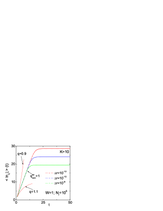
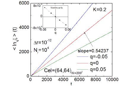
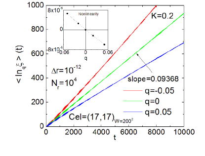
The correctness of this description can be checked, for both chaotic regimes of standard map, in Figures 1 and 4. They show, for different values of $q$, the averages of $\ln_{q}\xi(t)$ (where $\ln_{q}x\equiv(x^{1-q}-1)/(1-q)$ is the inverse function of the $q$-exponential, and $\ln_{1}x=\ln x$) over $N_{r}$ realizations. Each realization starts with a randomly chosen pair of very close initial conditions, that are localized inside a particular cell of the $W$ equally partitioned phase space. In Fig. 1, that corresponds to the case of strong chaos $K=10$, where LLE $>0$), we consider decreasing initial discrepancies in Eq. (2) so as to obtain a well defined behavior for increasingly long times. In all cases (strongly and weakly chaotic chaos), after a transient, we verify a nontrivial property ananos-tsallis-2004 namely that exists a special value of $q$, noted $q^{\text{av}}_{\text{sen}}$ (where av stands for average), which yields a linear dependence of $\langle\ln_{q_{\text{sen}}}\xi\rangle$ with time. In other words, we verify $\langle\ln_{q}\xi(t)\rangle\approx\lambda_{q_{\text{sen}}^{\text{av}}}t$.

For the strongly chaotic case, exponential sensitivity to the initial conditions is verified with $q_{\text{sen}}^{\text{av}}=1$, and the same generalized Lyapunov exponent characterizes the whole phase space no mater the value of $W$ or the particular cell to be chosen. Fig. 2 exemplifies this fact, as it shows that the slope of the temporal evolution of the averaged sensitivity to initial conditions is preserved over an intermediate regime where correlation coefficient equals one and $\lambda=\lambda_{q_{\text{sen}}^{\text{av}}=1}=1.62$ (time steps)^-1, in accordance with latora-baranger1999 . Consequently, generalized Lyapunov exponent does not depend on the spreading occupation index latora-baranger-tsallis-rapisarda-2000 of averaging cells, and it makes sense choosing the random pairs of initial conditions to compute the $N_{r}$ realizations all over the phase space, i.e. $W=1$.

Figure 1: (Color online) $\langle\ln_{q}\xi(t)\rangle$ vs. $t$, for $K=10$. The $N_{r}=10^{6}$ realizations are evaluated over the whole (not partitioned) phase space, i.e. $W=1$ (see text). Decreasing Euclidean distances between initial conditions $\Delta r\equiv\|{\bf\Delta x}(0)\|$ are considered. Linear dependence of $\langle\ln_{q_{\text{sen}}}\xi\rangle$ with time is yielded for $q^{\text{av}}_{\text{sen}}=1$.

Figure 2: (Color online) Left: Color map of the integrated number of occupied cells in a $W=500\times 500$ equally partitioned phase space, from iteration $1$ to iteration $10$, as a function of the $(x^{\text{th}},p^{\text{th}})$ localization of the cell that contains initial conditions. Right: Temporal evolution of $\langle\ln_{q=1}\xi\rangle$ for $K=10$, where $\Delta r\equiv\|{\bf\Delta x}(0)\|=10^{-12}$ is the Euclidean distance of the $N_{r}$ pairs of initial conditions. The $N_{r}=10^{6}$ realizations are estimated over one of the quickest spreading cells (the cell at line $248$ and column $27$, green squares) and over one of the slowest spreading cells (the cell at line $384$ and column $405$, black squares), amongst the $W=500\times 500$ cells of an equally partitioned phase space. Averaged temporal evolution $\langle\ln_{q=1}\xi(t)\rangle$ over the not partitioned phase space is also shown ($W=1$, red squares).

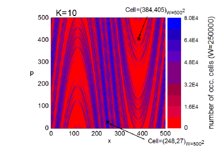
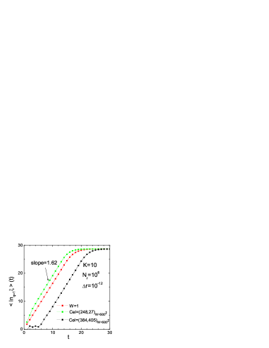
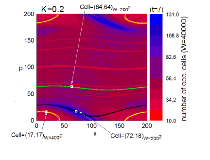
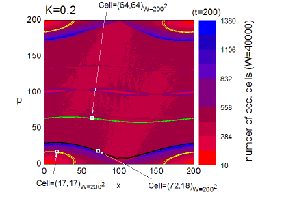
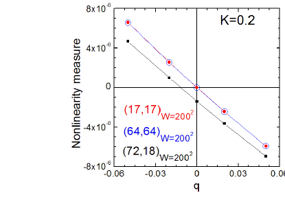
For the weakly chaotic case, stability islands dominate the phase space. Consequently, the characterization of the spreading occupation index of cells is much more intricate. In this case, a “global characterization” of the map has tentatively been made Baldovin-2002 ; Baldovin-2004 . But Fig. 3 ($K=0.2$, where LLE = $0$) demonstrates that a common transient time can not be defined, and this fact tends to preclude a neat linear dependence of $\langle\ln_{q_{\text{sen}}}\xi\rangle$ with time. We now do not choose the $N_{r}$ random pairs of initial conditions all over the phase space, but in particular cells, i.e., in local regions. Nevertheless, we identify regions that exhibit $q_{\text{sen}}^{\text{av}}=0$, whose value of $\lambda_{q_{\text{sen}}^{\text{av}}}$ depend on the initial cell, as shown in Figure 4. In fact, a huge set of randomly chosen cells exhibit analogous results of $q_{\text{sen}}^{\text{av}}=0$, but we have also found cells where linear behavior is satisfied for $q_{\text{sen}}^{\text{av}}\neq 0$ (Fig. 5).

Figure 3: (Color online) Color maps of the integrated number of occupied cells in a $W=200\times 200$ equally partitioned phase space, from iteration $1$ to iteration $t$ ($t=7$, left, $t=200$, right), as a function of the $(x^{\text{th}},p^{\text{th}})$ localization of the cell that contains the initial conditions. A set of quasi-periodic trajectories are superimposed to the maps, in order to warn about the different local transient times (yellow, black and green lines).

Figure 4: (Color online) Temporal evolution of $\langle\ln\xi_{q}\rangle$, when $K=0.2$, for $(64^{\text{th}},64^{\text{th}})$ (left figure) and $(17^{\text{th}},17^{\text{th}})$ (right figure) initial cells in the $W=200\times 200$ equally partitioned phase space. Averages are estimated for a set of $N_{r}=10^{4}$ realizations, whose initial conditions have been randomly chosen in their respective initial cells. The $(17^{\text{th}},17^{\text{th}})$ case presents a slightly periodically modulated evolution that is due to the not connected character of trajectories (see Fig. 3). Insets represent the nonlinearity measure $R\equiv C/B$ in the fitting curve of $\langle\ln\xi_{q}(t)\rangle$, $A+Bt+Ct^{2}$, and demonstrate that $q_{\text{sen}}^{\text{av}}=0$ is the optimum value of $q$ (a straight line fitting curve is obtained).

Figure 5: (Color online) Nonlinearity measure of the polynomial fitting curve $\langle\ln\xi_{q}(t)\rangle$ vs. $q$, for averages over $(17^{\text{th}},17^{\text{th}})$, $(64^{\text{th}},64^{\text{th}})$ and $(72^{\text{th}},18^{\text{th}})$ cells of the $W=200\times 200$ equally partitioned phase space of the standard map with $K=0.2$. Red and blue lines are superimposed.

III The rate of entropy production

With respect to the entropy production per unit time, we may conveniently use the $q$-entropy ($k=1$, henceforth) Tsallis1988 ; Tsallis2009

$$S_{q}(t)=k\frac{1-\sum_{i=1}^{W}p_{i}^{q}}{q-1}\qquad(S_{1}=S_{BG}=-k\sum_{i=1}^{W}p_{i}\ln p_{i}).$$ (5)

The $q$-entropy production is estimated dividing the phase space in $W$ equal cells, and randomly choosing $N_{\text{ic}}\gg W$ initial conditions inside one of the $W$ cells (typically $N_{\text{ic}}=10W$). We follow the spreading of points within the phase space, and calculate Eq. (5) from the set of occupancy probabilities $\{p_{i}(t)\}$ ($i=1,2,\dots,W$). Fluctuations are of course present, but they can be reduced when we choose $N_{c}\gg 1$ initial cells within which the $N_{\text{ic}}$ initial conditions are chosen, and average $S_{q}(t)$ over the $N_{c}$ realizations. The proper value of the entropic parameter $q_{\text{ent}}^{\text{av}}$ is the special value of $q$ which makes the averaged $q$-entropy production per unit time to be finite, which is ultimately related with the extensivity of the entropy. The $q$-entropy production per unit time is consequently obtained as

$$K_{q_{\text{ent}}^{\text{av}}}=\lim_{t\to\infty}\lim_{W\to\infty}\lim_{N_{\text{ic}}\to\infty}\frac{\langle S_{q_{\text{ent}}^{\text{av}}}(t)\rangle_{N_{c}}}{t}<\infty,$$ (6)

and must be calculated taking into account that the partitions of phase space, $N_{c}$ and $N_{\text{ic}}$ are such as to obtain robust results.

When the LLE is largely positive and the phase space is dominated by a chaotic sea, the Boltzmann-Gibbs entropy ($S_{1}=S_{BG}\equiv-\sum_{i=1}^{W}p_{i}\ln p_{i}$) is expected to be the appropriate one (i.e. $q_{\text{ent}}=1$). Our numerical results show, as expected, that the proper value of the entropic index is $q_{\text{ent}}^{\text{av}}=q_{\text{sen}}^{\text{av}}=1$ for $K=10$ (see Figure 6). Both indexes have been obtained comparing the nonlinearity measure of the polynomial fitting curves over the intermediate regime (after a transient and before saturation) were the correlation coefficient is constant and equals $1$. Another interesting result that emerged is the coincidence of the slopes of the sensitivity and entropy functions of time (see Fig. 2 and Fig. 6), i.e., the $q$-entropy production per unit time satisfies $K_{q_{\text{sen}}^{\text{av}}=1}=\lambda_{q_{\text{sen}}^{\text{av}}=1}$. These results are numerically compatible with a $q$-generalization of a Pesin-like identity for ensemble averages in strongly chaotic conservative maps, and reinforce those in ananos-tsallis-2004 .

Figure 6: (Color online) Temporal dependence of $(q_{\text{ent}}^{\text{av}}=1)$-entropy in the standard map with $K=10$, averaging over $1\%W$, for different values of the number of cells in the equally partitioned phase space, $W$. The case of $q<q_{\text{ent}}^{\text{av}}=1$ ($q>q_{\text{ent}}^{\text{av}}=1$) corresponds to positive (negative) concavity. The $t\to\infty$ limiting value is $\langle S_{1}\rangle=\ln W$.

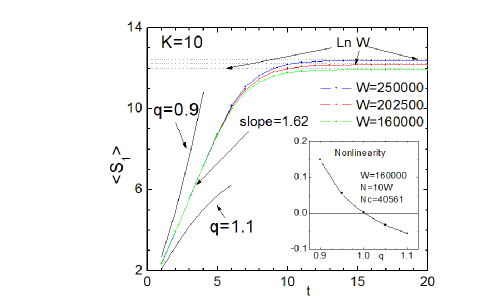
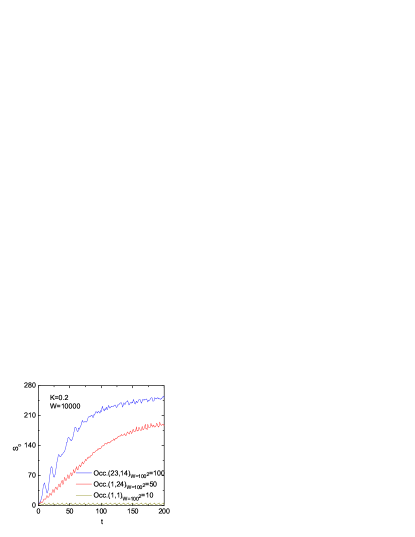
Entropic characterization of weak chaos regime in conservative maps is much more subtle than in dissipative maps (see Casati-Tsallis-Baldovin-2005 ; RuizTsallis ). First, let us notice that one of the practical difficulties to identify the weak chaos regime are the huge computer times required, because of the slow convergence of the finite time Larger Lyapunov Exponent to its $t\to\infty$ limit value. Furthermore, we know that the phase space of weakly chaotic conservative maps is dominated by stability islands and regions with a huge diversity of spreading occupation indexes, and this makes a hard task to reduce fluctuations by averaging the entropy. We have already pointed out that spreading occupation index of cells, and consequently their transient time scales, are essential in the $q$-sensitivity characterization of the map. Fig. 7 reveals the incidence of this phenomena on the entropy production, which is related to the sensibility to initial conditions, and we conclude that a smart averaging criterion must be adopted.

Figure 7: (Color online) $(q_{\text{ent}}^{\text{av}}=0)$-Entropy production of three representative cells in a $W=100\times 100$ equally partitioned phase space of the standard map with $K=0.2$. Their spreading occupation index from $t=1$ to $t=7$ are: Occ.$(23,14)=100$ (blue line), Occ.$(1,24)=50$ (red line), Occ.$(1,1)=10$ (brown line).

Initially we have tested the adequacy of the Smaller Alignment Index (SALI) Skokos to identify weak chaos in the $K=0.2$ standard map, so as to reduce the computer times required for LLE computation. We observe that the SALI temporal evolution is a computationally cheap tool to detect chaotic behavior of trajectories, as it tends to zero in both ordered and chaotic orbits, but with completely different time rates: SALI decreases abruptly in strongly chaotic orbits and reaches the limit of accuracy of the computer after about 200 iterations and, in contrast, it decreases with time as a power law in ordered orbits. We have verified, for the first time to the best of our knowledge, that the SALI decreases with time as a power law even in the case of weakly chaotic orbits. Fig. 8 shows, for the standard map with $K=0.2$, that the time required to characterize weak chaos of stability island is generically shorter if we study the SALI temporal evolution instead of the LLE $t\to\infty$ limit computation.

Figure 8: (Color online) Left: Paradigmatic stability island in phase space for the standard map with $K=0.2$, whose respective initial conditions are specified in the label. Center: Log-log representation of the respective finite time Larger Lyapunov Exponent. Right: Log-log representation of the respective SALI temporal evolution. The quasi-periodicity of trajectories are detected both by the $t\to\infty$ limit of LLE, and by the power-law behavior of the SALI temporal evolution.

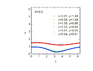
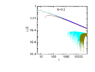
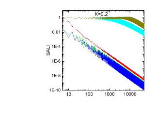
We then obtain the temporal production of the averaged entropy $\langle S_{q}\rangle_{N_{c}}$, selecting the $N_{c}$ cells between those that present analogous SALI temporal evolution: the smoother the log-log SALI evolution is, the smother its entropy production. This criterion provides averaged $q$-entropies, $\langle S_{q}\rangle_{N_{c}}$, that do not present the typical oscillations observed in conservative maps RuizTsallis . Fig. 9 exemplifies this fact.

Figure 9: (Color online) Increase of $(q_{\text{ent}}^{\text{av}}=0)$-entropy in the standard map with $K=0.2$, for different values of $W$, all over a longitudinal band of phase space that covers $p=2$ ($x\in[0,2\pi]$). The inset shows that $q<q_{\text{ent}}=0$ ($q>q_{\text{ent}}=0$) corresponds to positive (negative) concavity.

Summarizing, for weakly chaotic dissipative systems, particularly for the logistic map, it has been observed that there is a specific value of $q<1$ (for the logistic map, $q_{\text{ent}}=0.2445$ latora-baranger-tsallis-rapisarda-2000 ) which yields finite entropy production per unit time, and hence $S_{q_{\text{ent}}}$ ($q_{\text{ent}}<1$) is the proper one to thermodynamically characterize the system. Verification of this behavior for a conservative system (the standard map) is presently done. Our numerical results show in both strongly and weakly chaotic regime, as expected, $q_{\text{ent}}^{\text{av}}=q_{\text{sen}}^{\text{av}}$, and this points towards the conjecture of the generalized Pesin equality tsallis-plastino-zheng-1997 . In particular, $q_{\text{sen}}^{\text{av}}=q_{\text{ent}}^{\text{av}}=1$ and $K_{q_{\text{ent}}^{\text{av}}}=\lambda_{q_{\text{sen}}^{\text{av}}}=1.62$ for $K=10$ (strong chaotic regime, as $\lambda>0$), and $q_{\text{sen}}^{\text{av}}=q_{\text{ent}}^{\text{av}}=0$ for $K=0.2$ (weakly chaotic regime, as $\lambda=0$, $\lambda_{q_{\text{sen}}^{\text{av}}}>0$). With respect to the weakly chaotic regime, a local characterization of generalized Pesin-like remains to be made, as $K_{q_{\text{ent}}^{\text{av}}}$ and $\lambda_{q_{\text{sen}}^{\text{av}}}$ have both shown to be local properties.

IV The rate of relaxation of the entropy

The methods described in Sections II and III take an ensemble of initial conditions inside one of $W$ cells of the phase space, and thus $S_{q}(0)=0$, $\forall q$. In Ref. moura-tirnakli-lyra-2000 , the authors have considered an ensemble of initial conditions spread over the entire phase space of a dissipative system (particularly, the logistic map), therefore, with the maximum possible value for the entropy $S_{q_{\text{ent}}}(0)=\ln_{q_{\text{ent}}}W$. The time evolution brings the system to its attractor, and the number of occupied cells falls according to an exponential relation, in the case of a strongly chaotic system, or according to a $q$-exponential, in the case of a weakly chaotic system. Later it was found a relation between $q_{\text{rel}}$ and $q_{\text{ent}}$ by analyzing the rate in which the entropy goes to its final value, beginning with $S_{q_{\text{ent}}}(0)=0$, instead of $S_{q_{\text{ent}}}(0)=\ln_{q_{\text{ent}}}W$ ananos-borges-tsallis-oliveira-2002 .

The method adopted in moura-tirnakli-lyra-2000 cannot be identically applied to a conservative map, since there is no attractor, but that one introduced in ananos-borges-tsallis-oliveira-2002 can be adapted to area-preserving models. We consider the variable $\Delta S_{q}(t)=S_{q}(\infty)-S_{q}(t)$ and evaluate its average over an ensemble of initial conditions for $t\to\infty$. The average must be computed with a different criterion in strong and weak chaos regimes, according to the respective stability distributions on the phase space.

The strongly chaotic map is dominated all over the partitioned phase space by a chaotic sea, and we can analytically calculate $S_{q=1}(\infty)=\ln W$. In that case, the average $\langle\Delta S_{q}(t)\rangle_{N_{\text{ic}}}$ has been estimated over the most quickly spreading cells $N_{\text{ic}}$ to minimize the time computation. On the contrary, the stability islands dominate the phase space in the weakly chaotic regime, and their respective value of $S_{q_{\text{ent}}}(\infty)=\ln_{q_{\text{ent}}}W_{\text{islands}}$ is unknown, as it numerically depends on the cells where the initial conditions are randomly chosen. We must find a proper criterion for the numerical estimation of $S_{q_{\text{ent}}}(\infty)$ and $\langle\Delta S_{q}(t)\rangle_{W_{\text{islands}}}$, and we privilege those cells that cover a region were SALI behaves in a smoothly manner, such as to produce entropy in a smoothly manner too.

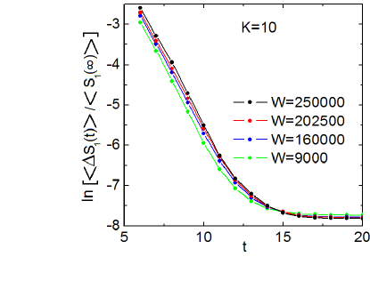
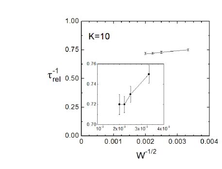
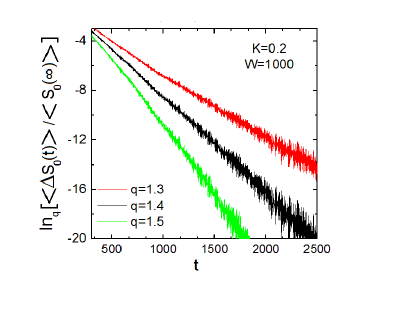
It is expected that $\displaystyle\lim_{W\to\infty}\Delta S_{q_{\text{ent}}^{\text{av}}}\sim\exp_{q_{\text{rel}}^{\text{av}}}(-t/\tau_{q})$, where $\tau_{q}$ is a relaxation time. Figures 10 and 11 show the time dependence of $\ln_{q_{\text{rel}}}\langle\Delta S_{q_{\text{ent}}}(t)\rangle/\langle S_{q_{\text{ent}}}(\infty)\rangle$ for the strongly chaotic case ($K=10$), and the weakly chaotic case ($K=0.2$), respectively. The former case displays an exponential relaxation, i.e., $q_{\text{rel}}=1$, consistently with BG framework. The weakly chaotic case presents a $q$-exponential relaxation regime, with $q_{\text{rel}}=1.4$ for $K=0.2$.

Figure 10: (Color online) Left: Time evolution of $\ln_{q_{\text{rel}}}\langle\Delta S_{q=1}(t)\rangle/\langle S_{q=1}(\infty)\rangle$ in the (strongly chaotic) standard map with $K=10$. The averages have been calculated over the more quickly spreading cells, to optimize the computational cost. Right: The numerical results of the inverse of relaxation time estimations, $\tau^{-1}_{\text{rel}}(W^{-1/2})$, to the $S_{q_{\text{ent}}=1}(\infty)$ entropy limit, are compatible with a finite relaxation time $\tau_{q=1}\equiv\tau_{\text{rel}}(W\to\infty)$.

Figure 11: (Color online) Time evolution of $\ln_{q_{\text{rel}}}\langle\Delta S_{q=0}(t)\rangle/\langle S_{q=0}(\infty)\rangle$ in the $K=0.2$ (weakly chaotic) standard map. The averages are calculated over the cells that belong to the same longitudinal band in phase space analyzed in Fig. 9. According to a procedure similar to what was done in Fig. 4 and 5, the nonlinearity measure identifies $q_{\text{rel}}=1.4$.

V Stationary distributions

Probability density distributions are among the most relevant items regarding the statistical description of dynamical systems. Gaussian distributions are typical for ergodic and mixing systems, for which LLE is positive tirnakli-beck-tsallis-2007 ; tirnakli-borges-2016 , and $q$-Gaussian distributions are typical for weakly chaotic systems for which LLE$\;=0$ tirnakli-beck-tsallis-2007 ; tirnakli-beck-tsallis-2009 ; tirnakli-borges-2016 and or chaotic layers are thin and LLE$\;\approx 0$ Ruiz-Bountis-tsallis-2012 .

We define the $q$-Gaussian distribution as

$$P_{q}(x;\mu_{q},\sigma_{q})=A_{q}\sqrt{B_{q}}\left[1-(1-q)B_{q}(x-\mu_{q})^{2}\right]^{\frac{1}{1-q}},$$ (7)

where $\mu_{q}$ is the $q$-mean value, $\sigma_{q}$ is the $q$-variance, $A_{q}$ is the normalization factor and $B_{q}$ is a parameter which characterizes the width of the distribution prato-tsallis-1999 :

$$A_{q}=\left\{\begin{array}[]{lc}\displaystyle\frac{\Gamma\left[\frac{5-3q}{2(1-q)}\right]}{\Gamma\left[\frac{2-q}{1-q}\right]}\sqrt{\frac{1-q}{\pi}},&q<1\\ \displaystyle\frac{1}{\sqrt{\pi}},&q=1\\ \displaystyle\frac{\Gamma\left[\frac{1}{q-1}\right]}{\Gamma\left[\frac{3-q}{2(q-1)}\right]}\sqrt{\frac{q-1}{\pi}},&1<q<3\end{array}\right.$$ (8)

$$B_{q}=[(3-q)\sigma_{q}^{2}]^{-1}$$ (9)

and where $q\to 1$ recovers the Gaussian distribution $P_{1}(x;\mu_{1},\sigma_{1})=\frac{1}{\sigma_{1}\sqrt{2\pi}}e^{-\frac{1}{2}\left(\frac{x-\mu_{1}}{\sigma_{1}}\right)^{2}}.$

Both Gaussian and $q$-Gaussian distributions have recently been observed for the standard map tirnakli-borges-2016 . We have analyzed the distribution of sums of iterates of the map, for representative $K$ values, as defined by

$$y=\sum_{i=1}^{T}(x_{i}-\langle x\rangle),$$ (10)

where the average $\langle\cdots\rangle$ is both a time average over $T$ iterations and an ensemble average over $M$ initial conditions:

$$\langle x\rangle=\frac{1}{M}\frac{1}{T}\sum_{j=1}^{M}\sum_{i=1}^{T}x_{i}^{(j)}.$$ (11)

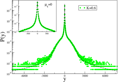
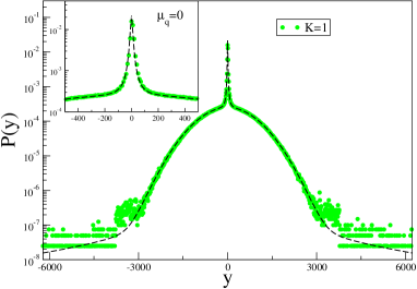
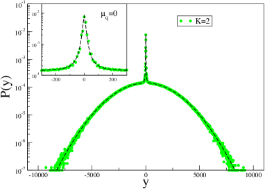
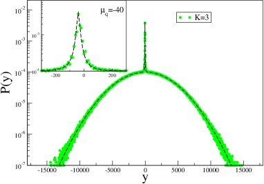
The probability distributions of $y$, namely $P(y)$, that emerge from the standard map with weakly chaotic phase space are $q$-Gaussians, while Gaussian distributions are associated with the strongly chaotic regime. The scenario for intermediate values of $K$ is also quite rich. For these cases, the phase space displays regions with points that have positive LLE, — the chaotic sea —, and regions with $\lambda=0$,— the stability islands. The probability distributions of $y$ for initial conditions taken inside the strongly chaotic regions are Gaussians, and those distributions for initial conditions that belong to the weakly chaotic regions are $q$-Gaussians. One remarkable feature is that $q_{\text{stat}}=1.935$ in all cases, regardless the value of $K$.

If the initial conditions are spread over the entire phase space, thus the initial conditions are from both the chaotic sea and the stability islands, the distribution that emerges is a linear combination of a Gaussian and a $q$-Gaussian. Consequently, the probability distribution of the standard map, for any arbitrary value of $K$, can be modeled as

$$P(y)=\alpha P_{q}(y;\mu_{q},\sigma_{q})+(1-\alpha)P_{1}(y;\mu_{1},\sigma_{1}).$$ (12)

where $P_{q}(y)$ and $P_{1}(y)$ are the probability densities of $y$ for the initial conditions taken inside the weak and strong chaos regions, respectively.

In Ref. tirnakli-borges-2016 it was taken the linear combination of the probability distributions normalized to the maximum value $P(0)$, and the physical meaning of the interpolating parameter was not clear. Now we have taken the linear combination of the usual probability densities in Eq. (12). We find out the ratio of the areas for the strongly and weakly chaotic regions. In order to achieve this, we randomly generate $N_{\text{ic}}=4\times 10^{6}$ initial conditions all over the phase space and count how many of those having non-zero Lyapunov and those having nearly zero Lyapunov. Dividing these numbers by the total number of initial conditions, we mimic the ratio of the areas. We classify an initial condition belonging to a weakly chaotic region if its Lyapunov exponent is smaller than a given threshold $\lambda<\lambda_{-}=5\times 10^{-5}$ (time steps)^-1. Correspondingly, an initial condition is considered to belong to a strongly chaotic region whenever $\lambda>\lambda_{+}=10^{-2}$ (time steps)^-1. These limiting values $\lambda_{-}$ and $\lambda_{+}$ are chosen according to what is explained in tirnakli-borges-2016 : the phase-space ratio, i.e., [number of points with $\lambda<\lambda_{\text{threshold}}$] / [number of points with $\lambda>\lambda_{\text{threshold}}$] remains almost constant for $\lambda_{-}<\lambda_{\text{threshold}}<\lambda_{+}$. We call $\alpha_{1}=N_{\text{ic}}(\lambda>\lambda_{+})/N_{\text{ic}}$, and $\alpha_{q}=N_{\text{ic}}(\lambda<\lambda_{-})/N_{\text{ic}}$. There remains a small amount of initial conditions with intermediate Lyapunov exponent values ($\lambda_{-}\leq\lambda\leq\lambda_{+}$) that are not taken into account in Eq. (12), and that are possibly negligible in the macroscopic limit. We have thus considered the approximated form of Eq. (12) as

$$P(y)\approx\alpha_{q}P_{q}(y;\mu_{q},\sigma_{q})+\alpha_{1}P_{1}(y;\mu_{1},\sigma_{1}).$$ (13)

See the results of some representative $K$ values in the Table.

$A_{1}=0.5642...$, $A_{q=1.935}=0.3364...$
$K$	$B_{1}$	$B_{q}$	$\alpha_{1}$	$\alpha_{q}$
0.2	$-$	0.015	0	1
0.6	$10.7\times 10^{-7}$	0.015	0.0380	0.9416
1	$8.00\times 10^{-7}$	0.015	0.4826	0.5078
2	$1.06\times 10^{-7}$	0.010	0.7622	0.2367
3	$0.40\times 10^{-7}$	0.010	0.8825	0.1170
10	$0.52\times 10^{-7}$	$-$	1	0

Table 1: The values of the parameters for representative $K$ values.

Then, we compute the $B_{1}$ and $B_{q}$ values using the pdf of the system coming from the initial conditions with positive and with zero Lyapunov values, respectively. After determining these values now we have no fitting parameter and $\alpha$ values are entirely determined by the intrinsic dynamics of the map. For some representative values of $K$, the results are given in Fig. 12.

Figure 12: (Color online) Probability distribution functions of the standard map for 4 representative $K$ values.

VI Concluding Remarks

The $q$-triplet ($q_{\text{ent}}$, $q_{\text{rel}}$, $q_{\text{stat}}$) is an important feature in the statistical description of dynamical systems that might be nonergodic and nonmixing, as a consequence of zero LLE. These indices define the rate of entropy production, the rate of relaxation, and the distribution of the stationary states. Positive LLE leads to ergodic, mixing systems, and strong chaos, and these indices collapse into $q=1$, within the BG framework. Zero LLE may lead to breakdown of ergodicity, nonmixing dynamics, and weak chaos. The statistical description in many such circumstances appears to be associated with the $q$-entropy, where the usual exponential and Gaussian functions turn into more general forms, namely the $q$-exponential and the $q$-Gaussian ones. This scenario has been previously observed and evaluated for dissipative low-dimensional systems.

We have now considered a paradigmatic low-dimensional conservative system, the standard map. We have evaluated the $q$-triplet, and have verified that the sensitivity to initial conditions index satisfies $q_{\text{sen}}=q_{\text{ent}}$, in both strongly and weakly chaotic regimes. Our results corroborate the expected situation, i.e., that if the phase space is completely strongly chaotic (LLE$>0$), $q_{\text{ent}}=q_{\text{rel}}=q_{\text{stat}}=1$ and $K_{q_{\text{ent}}^{\text{av}}}=\lambda_{q_{\text{sen}}^{\text{av}}=1}=1.62>0$. These results are numerically compatible with a $q$-generalization of a Pesin-like identity for ensemble averages, extending those in ananos-tsallis-2004 to the case of conservative maps. If the entire phase space is weakly chaotic regime ($\lambda\approx 0$), which happens for low values of $K$, the standard map is characterized by $q_{\text{ent}}=0$, $q_{\text{rel}}\simeq 1.4$, and $q_{\text{stat}}\simeq 1.935$. We have shown that $\lambda_{q_{\text{sen}}^{\text{av}}}$ is a property that can be locally characterized by the finite temporal evolution of LLE or, alternatively, by the SALI, which has demonstrated to be a computationally cheaper tool to identify different chaotic regimes. The phase space for intermediate values of $K$ features regions of positive and regions of zero LLE. Ensemble averages of initial conditions taken within the strongly chaotic regions behave according to $q_{\text{ent}}=q_{\text{rel}}=q_{\text{stat}}=1$. In contrast, ensemble averages of initial conditions taken within the weakly chaotic regions behave according to the $q$-triplet and, at least in what concerns the stationary distribution, with the same values of $q_{\text{stat}}$. This work extends what has been done in Ref. tirnakli-borges-2016 . We have numerically found the proper superposition of distributions for the mixed case (coexistence of strongly and weakly chaotic regimes) without any additional fitting parameter.

The $q$-triplet structure plays a central role on the statistical description of dynamical systems, and additional works addressing other conservative and dissipative maps shall bring further tests for the robustness of this framework, and they are very welcome.

References

- (1) C. Tsallis, Introduction to Nonextensive Statistical Mechanics – Approaching a Complex World (Springer, New York, 2009).
- (2) C. Beck and F. Schlögl, Thermodynamics of chaotic systems – An introduction (Cambridge Nonlinear Science, 1997).
- (3) A. Rapisarda and V. Latora, in Nonextensive Entropy - Interdisciplinary Applications, Edited by Gell-Mann, C. Tsallis (Oxford University Press, New York, 2004).
- (4) A. Esquivel and A. Lazarian, ApJ 710, 125 (2010).
- (5) CMS Collaboration, Phys. Rev. Lett. 105, 022002 (2010).
- (6) M. Shao, L. Yi, Z. Tang, H. Chen, C. Li and Z. Xu, J. Phys. G Nucl Partic 37, 085104 (2010).
- (7) O. Sotolongo-Grau, D. Rodríguez-Pérez, J. C. Antoranz and O. Sotolongo-Costa, Phys. Rev. Lett. 105, 158105 (2010).
- (8) Mohanalin, Beenamol, P. K. Kalra and N. Kumar, Comput. Math. Appl. 60, 2426 (2010).
- (9) ALICE Collaboration, Phys. Lett. B 693, 53 (2010).
- (10) PHENIX Collaboration, Phys. Rev. D 83, 052004 (2011).
- (11) PHENIX Collaboration, Physical Review C 83, 024909 (2011).
- (12) ALICE Collaboration, Eur. Phys. J. C C 71, 1655 (2011).
- (13) ATLAS Collaboration, New J. Phys. 13, 053033 (2011).
- (14) C. Y. Wong and G. Wilk, Phys. Rev. D 87, 114007 (2013)
- (15) L. Marques, E. Andrade-II and A. Deppman, Phys. Rev. D 87, 114022 (2013)
- (16) M. I. Bogachev, A. R. Kayumov and A. Bunde, PLoS ONE 9, e112534 (2014).
- (17) G. Combe, V. Richefeu, M. Stasiak and A. P. F. Atman, Phys. Rev. Lett. 115, 238301 (2015).
- (18) F. Baldovin and A. Robledo, Phys. Rev. E 66, 045104(R) (2002).
- (19) G. L. Ferri, M. F. Reynoso Savio and A. Plastino, Physica A 389, 1829 (2010).
- (20) L. F. Burlaga and N. F. Ness, Astrophys. J. 765, 35 (2013).
- (21) B. V. Chirikov, Phys. Rep. 52, 264 (1979).
- (22) G. M. Zaslavsky, Hamiltonian Chaos and Fractional Dynamics (Oxford University Press, New York, 2005).
- (23) G. Benettin, L. Galgani, A. Giorgilli and J.-M. Strelcyn, Meccanica 15, 9 (1980).
- (24) U. Tirnakli and E. P. Borges, Sci. Rep. 6, 23644 (2016).
- (25) M. Baranger, V. Latora, and A. Rapisarda, Chaos, Solitons & Fractals 13, 471 (2002)
- (26) C. Tsallis, A. R. Plastino and W.-M. Zheng, Chaos, Solitons & Fractals 8, 885 (1997)
- (27) C. Tsallis, Quimica Nova 17, 468 (1994).
- (28) G. F. J. Añaños and C. Tsallis, Phys. Rev. Lett. 93, 020601 (2004).
- (29) V. Latora and M. Baranger, Phys. Rev. Lett. 82, 520 (1999).
- (30) V. Latora, M. Baranger, A. Rapisarda and C. Tsallis, Phys. Lett. A 273, 97 (2000).
- (31) F. Baldovin, Physica A 305, 124 (2002).
- (32) F. Baldovin, in Nonextensive Entropy - Interdisciplinary Applications, Edited by Gell-Mann, C. Tsallis (Oxford University Press, New York, 2004).
- (33) C. Tsallis, J. Stat. Phys. 52, 479 (1988).
- (34) G. Casati, C. Tsallis and F. Baldovin, Europhys. Lett. 72, 355 (2005).
- (35) G. Ruiz and C. Tsallis, Physica A 386, 720 (2007).
- (36) Ch. Skokos, J. Phys. A: Math. Gen. 34, 10029 (2001).
- (37) F. A. B. F. de Moura, U. Tirnakli and M. L. Lyra, Phys. Rev. E 62, 6361 (2000).
- (38) E. P. Borges, C. Tsallis, G. F. J. Añaños, and P. M. C. de Oliveira, Phys. Rev. Lett. 89, 254103 (2002).
- (39) U. Tirnakli, C. Beck and C. Tsallis, Phys. Rev. E 75, 040106(R) (2007).
- (40) U. Tirnakli, C. Tsallis and C. Beck, Phys. Rev. E 79, 056209 (2009).
- (41) G. Ruiz, T. Bountis and C. Tsallis, Int. J. Bif. and Chaos 22, 1250208 (2012).
- (42) D. Prato, C. Tsallis, Phys. Rev. E 60, 2398 (1999).