Chaos and regularity in the doubly magic nucleus 208Pb
Abstract
High resolution experiments have recently lead to a complete identification (energy, spin, and parity) of 151 nuclear levels up to an excitation energy of MeV in 208Pb [Heusler et al., Phys. Rev. C 93, 054321 (2016)]. We present a thorough study of the fluctuation properties in the energy spectra of the unprecedented set of nuclear bound states. In a first approach we grouped states with the same spin and parity into 14 subspectra, analyzed standard statistical measures for short- and long-range correlations, i.e., the nearest-neighbor spacing distribution, the number variance , the Dyson-Mehta statistics, and the novel distribution of the ratios of consecutive spacings of adjacent energy levels in each energy sequence and then computed their ensemble average. Their comparison with a random matrix ensemble which interpolates between Poisson statistics expected for regular systems and the Gaussian Orthogonal Ensemble (GOE) predicted for chaotic systems shows that the data are well described by the GOE. In a second approach, following an idea of Rosenzweig and Porter [Phys. Rev. 120, 1698 (1960)] we considered the complete spectrum composed of the independent subspectra. We analyzed their fluctuation properties using the method of Bayesian inference involving a quantitative measure, called the chaoticity parameter , which also interpolates between Poisson () and GOE statistics (). It turns out to be . This is so far the closest agreement with GOE observed in spectra of bound states in a nucleus. The same analysis has also been performed with spectra computed on the basis of shell model calculations with different interactions (SDI, KB, M3Y). While the simple SDI exhibits features typical for nuclear many-body systems with regular dynamics, the other, more realistic interactions yield chaoticity parameters close to the experimental values.
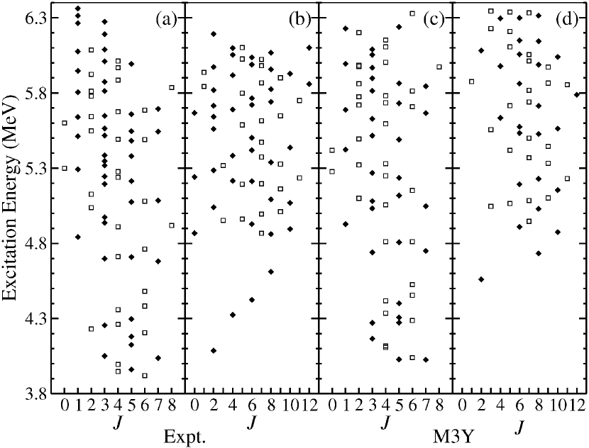
Introduction.– The stable doubly magic nucleus 208Pb is one of the most studied nuclei both experimentally and theoretically. Many of its spectral properties are basically understood in terms of the nuclear shell model. In recent years, however, a number of high resolution experiments using various types of nuclear reactions have been performed P.All6.2MeV ; NDS2007 ; P.s1p3 ; 11th_Heu . The foremost result is that now the complete level scheme in 208Pb is established up to an excitation energy of MeV comprising 151 bound states, of which the energy, spin, and parity have been unambiguously determined P.All6.2MeV . More states with spin and parity are known up to MeV NDS2007 ; P.s1p3 ; 11th_Heu . In Fig. 1 the experimental levels are shown separately for states of negative (a) and positive (b) parity for a range of excitation energies MeV. Levels corresponding to states with natural and unnatural parity are shown as filled diamonds and open squares, respectively.
The level scheme of 208Pb has also been the subject of many shell model calculations of the one-particle one-hole and two-particle two-hole type KuoBrown1968 ; KuoB66 ; Kuo1967 ; Kuo197093 ; PhysRevC.3.2421 ; Gillet196444 ; 2000Brwn ; KHMaier2007 ; Bertsch1977 ; PhysRevC.26.1323 ; P.mSM_Jolos ; Mosz1979 ; Talmi1993 . Mostly, the coupling of proton particles in the orbitals , , , , , to proton holes in the orbitals , , , , , and the coupling of neutron particles in the orbitals , , , , , , to neutron holes in the orbitals , , , , , were taken into account; see, e.g., Fig. 1 of Ref. Warburton1991 , however, note the different labelings used for the main quantum number. For detailed level schemes of the relevant proton and neutron orbits in the four neighboring nuclei of 208Pb see, e.g., Fig. 1 in P.All6.2MeV or Fig. 3-3 in BM1969 . The calculations of Kuo and Brown (KB) use four additional orbitals KuoBrown1968 ; KuoB66 ; Kuo1967 ; Kuo197093 . In total, there are 27 different combinations of spin and parity for one-particle one-hole states in 208Pb. The surface-delta interaction (SDI), which acts only at the nuclear surface, has been introduced as a simple extension of the schematic shell model without residual interaction. The associated interaction strength depends on the atomic mass number as the ratio of the surface to the volume term and on geometrical recoupling coefficients Mosz1979 ; Talmi1993 ; P.mSM_Jolos . The KB interaction is based on the free nucleon-nucleon potential of Hamada and Johnston KuoBrown1968 ; KuoB66 ; Kuo1967 ; Kuo197093 and the more recent two-body Michigan-three-Yukawas (M3Y) interaction on a one-boson exchange potential with short-range components determined with the help of the Reid nucleon-nucleon potential KHMaier2007 ; Bertsch1977 ; PhysRevC.26.1323 . Figure 1 shows the excitation energies calculated with the shell model which employs the effective nucleon-nucleon interaction M3Y for negative (c) and positive (d) parity.
The main objective of the present Letter is not a level by level comparison, but rather a comparison of the spectral properties of the whole set of detected bound states in 208Pb up to an excitation energy of MeV, which is still about one MeV below the neutron threshold ( MeV), and of the three theoretical models with Random Matrix Theory (RMT) results. For a generic quantum system with classically regular dynamics the spectral properties are predicted to coincide with those of Poissonian random numbers Berry1977 . According to the Bohigas-Giannoni-Schmit conjecture PhysRevLett.52.1 the spectral properties of time-reversal invariant chaotic systems are well described by those of the eigenvalues of real-symmetric matrices with Gaussian distributed random entries from the GOE McDonald1979 ; Casati1980 ; Berry1981 ; Dyson1963 ; Mehta1990 . These features are also observed in nuclear many-particle systems with no obvious classical analogue. Their spectral properties are described by Poissonian statistics, if the motion of the particles is collective, whereas for sufficiently complex motion they exhibit GOE statistics Guhr1989 ; Flambaum1994 ; Zelevinsky1996 ; Gomez2011 . There are various methods to obtain information on the chaoticity vs. regularity in a nuclear many-body system from its spectrum, see e.g. the review articles RevModPhys.81.539 ; Gomez2011 . We analyzed the fluctuation properties of the energy levels using two models, where one is based on a RMT ensemble Lenz1991 ; Alt1993 ; Kota2014 and the other one on the method of Bayesian inference Abul1996 ; Abul2004 ; Abul2006 . Both provide quantitative measures for the chaoticity in terms of a parameter which interpolates between the Poisson statistics and GOE statistics.
Spectral data.– We note that besides for 208Pb, there are to our knowledge only two other nuclei for which complete level schemes exist, namely 26Al and 30P Mitchell1988 ; Shriner2005 ; 1402-4896-2001-T90-015 . That of 116Sn has been termed “nearly complete” by the authors of Ref. Raman1991 ; Garrett1997 . Furthermore, the analysis of the spectral properties of experimentally determined bound states of nuclei did not yield the results expected in nuclear many-body systems exhibiting a chaotic dynamics. For light nuclei this was attributed to the insufficient number of identified bound states, and for nuclei like 26Al and 30P to the partial isospin symmetry breaking Mitchell1988 ; Shriner2005 . The present analysis of the experimental data is based on the 151 bound states with unambiguously assigned parity and spin P.All6.2MeV , so the results are statistically significant.
We applied two different approaches to analyze the spectral fluctuation properties of the experimental data P.All6.2MeV ; NDS2007 ; P.s1p3 ; 11th_Heu and calculations KuoBrown1968 ; KuoB66 ; Kuo1967 ; Kuo197093 ; PhysRevC.3.2421 ; Gillet196444 ; 2000Brwn ; KHMaier2007 ; P.mSM_Jolos ; Mosz1979 ; Talmi1993 . In the first approach we determined the ensemble averages of the statistical measures for the spectral properties of each level sequences Bohigas1983 characterized by spin and parity. In the second approach we followed an idea of Rosenzweig and Porter PhysRev.120.1698 and considered the complete spectrum composed of the independent subspectra and analyzed their fluctuation properties using the method of Bayesian inference. Note, that the spectral properties are Poissonian, when we use the complete experimental spectrum irrespective of parity and spin, see Fig. 6 of Sec. I. In both approaches we considered only subspectra that contained at least 5 levels. Furthermore, we first unfolded the energy levels in each sequence individually by replacing them by the smooth part of the integrated level density, yielding a mean spacing of unity, . The latter was determined from a fit of a third order polynomial to the integrated level density. In order to assure ourselves, that the spectral properties do not depend on the unfolding procedure, we, in addition unfolded the energy levels using an empirical formula Cameron1965 ; Gilbert1965 , with and the fit parameters. It was applied to low-lying nuclear levels in Ref. Shriner1991 . We came to the result that both procedures yield very similar results for the fluctuations of the energy levels.
Ensembles of subspectra.– In order to get information on the chaoticity of the nuclear many-body system we calculated for each sequence of unfolded levels (i) the nearest-neighbor spacing distribution (NNSD) , (ii) the number variance , (iii) the Dyson-Mehta statistics Dyson1963 ; Mehta1990 which gives the least-square deviation of the integrated level density from the best-fit straight line, and (iv) the distribution of the ratios of the consecutive spacings of adjacent energy levels Atas2013 ; Dietz2016 which has the advantage that the energy levels need not be unfolded. The corresponding analytical expressions for Poisson and GOE statistics are given in Refs. Dyson1963 ; Mehta1990 ; Atas2013 .
We analyzed the statistical measures for the experimental energy levels and for the levels obtained from nuclear model calculations using the SDI, M3Y, and KB interactions for each of the subspectra separately and subsequently computed their ensemble averages, where the values of are given in Tab. 1. Then we compared them to those of random matrices from an ensemble interpolating between Poisson and GOE Lenz1991 ; Kota2014 ,
| (1) |
where is a diagonal matrix of random Poissonian numbers and is a matrix from the GOE. Here, the range of values of the entries of coincided with that of the eigenvalues of . Furthermore, the variances of the matrix elements of and were chosen such that the mean spacings of their eigenvalues equaled unity, respectively. For , the statistics is Poissonian, whereas for the statistical properties are close to those of random matrices from the GOE. In Ref. Lenz1991 a Wigner-like approximation was derived for the NNSD using random matrices. It is given in terms of the Bessel function and the Kummer function as
| (2) | |||||
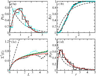
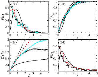
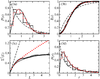
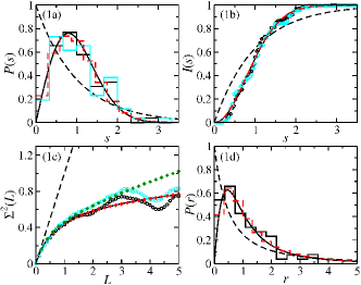
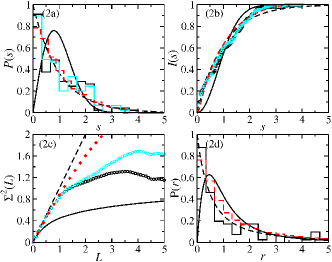
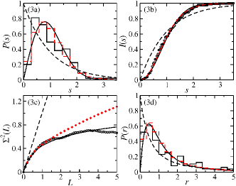
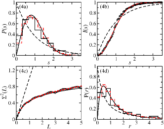
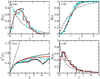
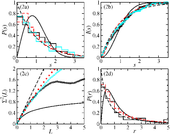
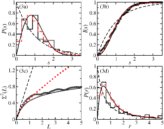
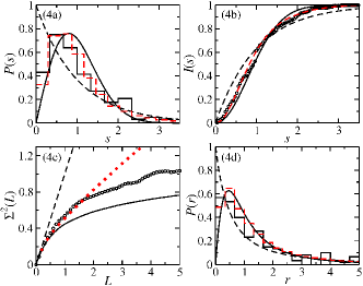
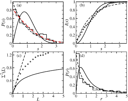
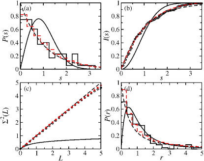
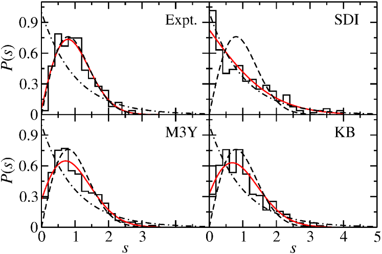
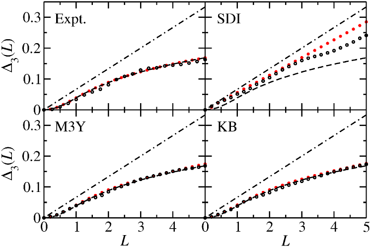
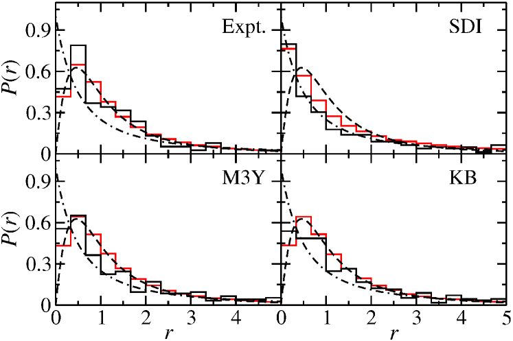
with . In order to determine the parameters for the experimental and calculated spectra, we fit this expression to their NNSDs and also compared their -statistics with that obtained for the RMT model Eq. (1) around the respective values. Inclusion of long-range correlations turned out to be crucial for the determination of the best-fit parameters. The values and the mean-square deviation of the respective NNSD from the analytical one, , are given in the last two columns in the rows termed “all” in Table 1. We repeated the analysis taking into account only levels with positive, negative, natural () and unnatural () parity, respectively. This analysis clearly revealed that the spectral properties of the experimental levels are very close to GOE. The NNSDs for the M3Y and the KB interaction models are also close to GOE, however, their statistics hint at a slightly larger contribution from regular behavior than for the experimental ones. Interestingly, for all these cases the spectra of levels with positive or natural parity are closer to GOE than those with negative and unnatural parity, respectively. The SDI model, on the contrary, clearly exhibits Poissonian features. We illustrate the findings in Figs. 2-4 where we compare the NNSD, the statistics and the ratio distributions of the experimental and calculated levels (histograms and circles) with those of Poissonian random numbers (dash-dotted lines) and of random matrices from the GOE (dashed lines). Furthermore, Figs. 3 and 4 show the results (red histogram and dots) obtained from the RMT model Eq. (1) using the values given in Table 1; see also Figs. 1-3 of Ref. Sec. I. A second measure for the chaoticity vs. regularity is analyzed in the next section.
| Model | Parity | ||||||
|---|---|---|---|---|---|---|---|
| Expt. | all | 14 | 128 | 0.95 | 0.015 | 1.50 | 0.060 |
| SDI | all | 13 | 262 | 0.18 | 0.069 | 0.08 | 0.001 |
| M3Y | all | 13 | 282 | 0.73 | 0.066 | 0.64 | 0.053 |
| KB | all | 14 | 257 | 0.62 | 0.070 | 0.60 | 0.074 |
| Expt. | 7 | 45 | 0.94 | 0.033 | 1.70 | 0.140 | |
| SDI | 6 | 82 | 0.05 | 0.042 | 0.01 | 0.010 | |
| M3Y | 6 | 84 | 0.84 | 0.079 | 1.13 | 0.081 | |
| KB | 4 | 62 | 0.88 | 0.059 | 1.50 | 0.118 | |
| Expt. | 7 | 83 | 0.87 | 0.091 | 0.70 | 0.093 | |
| SDI | 7 | 180 | 0.10 | 0.062 | 0.05 | 0.025 | |
| M3Y | 7 | 198 | 0.66 | 0.085 | 0.64 | 0.057 | |
| KB | 10 | 295 | 0.62 | 0.070 | 0.50 | 0.079 | |
| Expt. | nat. | 5 | 79 | 0.92 | 0.051 | 1.20 | 0.096 |
| SDI | nat. | 7 | 136 | 0.16 | 0.087 | 0.05 | 0.001 |
| M3Y | nat. | 7 | 147 | 0.80 | 0.073 | 0.75 | 0.094 |
| KB | nat. | 7 | 169 | 0.74 | 0.091 | 1.10 | 0.085 |
| Expt. | unnat. | 6 | 49 | 0.89 | 0.084 | 2.00 | 0.120 |
| SDI | unnat. | 6 | 126 | 0.09 | 0.063 | 0.10 | 0.001 |
| M3Y | unnat. | 6 | 135 | 0.65 | 0.096 | 0.58 | 0.089 |
| KB | unnat. | 6 | 188 | 0.62 | 0.088 | 0.50 | 0.079 |
Superimposed subspectra.– For the analysis of the composite spectra we proceeded as described in Abul1996 ; Abul2004 ; Abul2006 . Accordingly, we first computed the spacings between adjacent unfolded energy levels in each subspectrum separately, and then merged them irrespective of spin and parity into one sequence of spacings with given in 1. An approximate expression was derived for the NNSD of a spectrum composed of subspectra with fractional level numbers in Ref. PhysRev.120.1698 . In Ref. Abul1996 an approximation was derived which depends only on one parameter and is given by
| (3) |
with . Note, that for , which corresponds to a spectrum composed of a large number of subspectra consisting of a few number of levels, this distribution approaches the Poisson distribution, whereas for it converges to the NNSD of the GOE. Therefore, is referred to as chaoticity parameter.
In order to determine the values of for the experimental and calculated composite spectra, we used the method of Bayesian inference Harney2003 . Assuming that the spacings are statistically independent, their joint probability distribution can be written as the product
| (4) |
where we used the notation and is given by Eq. (3). The assumption, actually, restricts the applicability of the approach to short-range correlation functions. According to Bayes’ theorem the posterior distribution of the parameter for a given sequence of spacings is given as
| (5) |
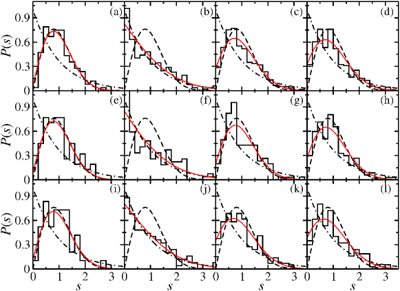
where is the prior distribution of and is the normalization constant. Using Jeffrey’s rule Jeffrey1946 ; Jeffrey1961 ; Harney2003 , an approximate expression was derived for in Ref. Abul2004 , . To determine the chaoticity parameter , we computed the joint probability distribution of the spacings for using Eq. (3). The best-fit value of was then obtained as the mean value , which gives the fraction of subspectra that exhibit GOE behavior with variance , , where provides a measure for the uniformity of chaoticity in the ensemble of subspectra. This yielded the values of and listed in Table 1 for the experimental and calculated spectra. They are in line with those obtained with the RMT model Eq. (1). The corresponding NNSDs are shown as red curves in Fig. 2 and in Fig. 4 of Sec. I.
Results, discussion, and conclusion.– Table 1 summarizes the results of the analysis of the recently completed level scheme of 208Pb at MeV together with complementary results rom calculations. For the experimental and the calculated spectra of the nuclear models with M3Y and KB interactions denoted “all” in Table 1, the chaoticity parameters and indicate that the spectral properties are described by GOE, even though there seems to be some small admixture from regular dynamics in the latter two cases. The chaoticity parameters for the SDI, on the contrary, suggest a behavior which is close to Poisson statistics. In a second step the same analysis has been applied to the spectra of energy levels with positive, negative, natural and unnatural parity, respectively. Albeit the sample sizes of and are smaller, the chaoticity parameters for the experimental spectra and for those calculated with the M3Y and KB interactions again are close to the values of GOE statistics. Note, that the parameters are closer to that for a pure GOE for levels with positive and natural parity than for those with negative and unnatural parity. In contrast, all chaoticity parameters obtained for the SDI interaction are compatible with regularity. We may conclude that the SDI, which provides a simple extension of the schematic shell model P.mSM_Jolos , does not describe the underlying interactions in the nucleus 208Pb correctly. On the other hand, the M3Y and KB interactions are based on realistic, effective nucleon-nucleon interactions.
However, especially our finding for the levels with unnatural parity differs from those of an analysis of the NNSD based on the same experimental data P.All6.2MeV in terms of the Brody distribution Brody1981 which also depends on a chaoticity parameter Munoz2016 . These discrepancies might orginate from the fact that the analysis of Ref. Munoz2016 did not include long-range correlations. Nevertheless, we obtain chaoticity parameters close to the values for GOE even when taking into account only the NNSD. To ensure, that this discrepancy does not arise from the unfolding procedure, we furthermore evaluated the ratio distributions using ensembles of subspectra comprising the natural and unnatural parity states, respectively. This analysis corroborated the outcome of the calculations with the RMT model Eq. (1) and the method of Bayesian inference.
In conclusion, by analyzing a complete set of levels in 208Pb with unambiguously assigned spin and parity with the RMT model Eq. (1) and the Bayesian method evidence has been presented for fluctuation properties which are consistent with those of random matrices from the GOE, thus for chaoticity of the nuclear system. Similar results where obtained from the analysis of the spectra generated from nuclear model calculations with M3Y and KB interactions. These two models confirm that the chaoticity is caused by a nuclear residual interaction that mixes the configurations inextricably in the many-body system. Indeed, e.g., in the M3Y model, the spectral properties of the unperturbed enegery levels, i.e., the diagonal elements of the Hamiltonian , yielded for the chatocity parameters and , respectively, that is they exhibit Poisson statistics, see Fig. 5 of Sec. I. These values, actually, are close to those for the SDI interaction. Furthermore, the distance between the unperturbed energy levels for each value of , and the perturbed ones, i.e., the eigenvalues of , is considerably larger than the root-mean square of the off-diagonal interaction matrix elements of ; see chapter 4 of Ref. Guhr1998 . Thus, the SDI interaction seems to be too weak to induce a sufficient mixture of the individual configurations to yield a chaotic dynamics.
Acknowledgements.
We thank T. Guhr, T. T. S. Kuo, and H. A. Weidenmüller for discussions. One of us (A. R.) is grateful to L. Muñoz for providing the article Munoz2016 prior to publication. This work was supported by the Deutsche Forschungsgesellschaft (DFG) within the Collaborative Research Centers 634 and 1245. BAB acknowledges U.S. NSF Grant No. PHY-1404442.References
- [1] A. Heusler, R. V. Jolos, T. Faestermann, R. Hertenberger, H.-F. Wirth, P. von Brentano, Phys. Rev. C 93, 054321 (2016).
- [2] M. J. Martin, Nucl. Data Sheets 108, 1583 (2007).
- [3] A. Heusler, T. Faestermann, R. Hertenberger, R. Krücken, H.-F. Wirth, P. von Brentano, Eur. Phys. J. A 46, 17 (2010).
- [4] A. Heusler, J. Phys.: Conf. Ser., 580, 012021 (2015).
- [5] T. T. S. Kuo and G. E. Brown, Privately communicated tables of wave functions, (1968). https://www.mpi-hd.mpg.de/personalhomes/hsl/Blei208KuoBrown/
- [6] T. T. S. Kuo and G. E. Brown, Nucl. Phys. 85, 40 (1966).
- [7] T. T. S. Kuo, Nucl. Phys. A 193, 71 (1967).
- [8] T. T. S. Kuo, J. Blomqvist, G. E. Brown, Phys. Lett. B 31, 93 (1970).
- [9] W. W. True, C. W. Ma, W. T. Pinkston. Phys. Rev. C 3, 2421 (1971).
- [10] V. Gillet, A. M. Green, and E. A. Sanderson. Phys. Lett. 11, 44 (1964).
- [11] B. A. Brown, Phys. Rev. Lett. 85, 5300 (2000).
- [12] K. H. Maier, (2007). https://www.mpi-hd.mpg.de/personalhomes/hsl/Blei208KHMaier/
- [13] G. Bertsch, J. Borysowicsz, H. McManus, and W. G. Love, Nucl. Phys. 284, 399 (1977).
- [14] G. F. Bertsch and I. Hamamoto, Phys. Rev. C 26, 1323 (1982).
- [15] A. Heusler, R. V. Jolos, and P. von Brentano. Yad. Fiz. 76, 860 (2013), [Phys. Atomic Nuclei 76, 807 (2013)]. https://www.mpi-hd.mpg.de/personalhomes/hsl/Blei208SDI/
- [16] S. A. Moszkowski, Phys. Rev. C 19, 2344 (1979).
- [17] I. Talmi, Simple Models of Complex Nuclei, in Contemporary Concepts in Physics, Vol. 7. Harwood Ac. Publ., Chur (Switzerland), (1993).
- [18] E. K. Warburton and B. A. Brown, Phys. Rev. C 43, 602 (1991).
- [19] A. Bohr and B. R. Mottelson, Nuclear Structure, Vol I. W. A. Benjamin, New York, (1969).
- [20] M. V. Berry and M. Tabor, Proc. R. Soc. A 356, 375 (1977).
- [21] O. Bohigas, M. J. Giannoni, and C. Schmit, Phys. Rev. Lett. 52, 1 (1984).
- [22] S. W. McDonald and A. N. Kaufman, Phys. Rev. Lett. 42, 1189 (1979).
- [23] G. Casati, F. Valz-Gris, and I. Guarneri. Lett. Nuovo. Cim. 28, 279 (1980).
- [24] M. V. Berry, J. Phys. 2, 91 (1981).
- [25] F. J. Dyson and M. L. Mehta, J. Math. Phys. 4, 701 (1963).
- [26] M. L. Mehta, Random Matrices, Acad. Press, London, (1990).
- [27] T. Guhr and H. A. Weidenmüller, Ann. Phys. 193, 472 (1989).
- [28] V. V. Flambaum, A. A. Gribakina, G. F. Gribakin, and M. G. Kozlov, Phys. Rev. A 50, 268 (1994).
- [29] V. Zelevinsky, B. A. Brown, N. Frazier, and M. Horoia, Phys. Rep. 276, 85 (1996).
- [30] J. M. G. Gómez, K. Kar, V. K. B. Kota, R. A. Molina, A. Relaño, and J. Retamosa , Phys. Rep. 499, 103 (2011).
- [31] H. A. Weidenmüller and G. E. Mitchell, Rev. Mod. Phys. 81, 539 (2009).
- [32] G. Lenz and F. Haake, Phys. Rev. Lett. 67, 1 (1991).
- [33] H. Alt, H.-D. Gräf, H. L. Harney, R. Hofferbert, H. Lengeler, C. Rangacharyulu, A. Richter, and P. Schardt, Phys. Rev. E 50, R1 (1994).
- [34] V. K. B. Kota, Lecture Notes in Physics 884 (Springer, Heidelberg, 2014).
- [35] A. Y. Abul-Magd and M. H. Simbel, Phys. Rev. C 54, 1675 (1996).
- [36] A. Y. Abul-Magd, H. L. Harney, M. H. Simbel, and H. A. Weidenmüller, Phys. Lett. B 579, 278 (2004).
- [37] A. Y. Abul-Magd, H. L. Harney, M. H. Simbel, and H. A. Weidenmüller, Ann. Phys. (N.Y.) 321, 56 (2006).
- [38] G. E. Mitchell, E. G. Bilpuch, P. M. Endt, and J. F. Shriner, Jr., Phys. Rev. Lett. 61, 1473 (1988).
- [39] J. F. Shriner, Jr., G. E. Mitchell, and B. A. Brown, Phys. Rev. C 71, 024313 (2005).
- [40] G. E. Mitchell and J. F. Shriner Jr, Phys. Scr. T 90, 105 (2001).
- [41] S. Raman,T. A. Walkiewicz, S. Kahane, E. T. Jurney, J. Sa, Z. Gácsi, J. L. Weil, K. Allaart, G. Bonsignori, J. F. Shriner Jr, Phys. Rev. C 43, 521 (1991).
- [42] J. D. Garrett, J. Q. Robinson, A. J. Foglia, H.-Q. Jin, Phys. Lett. B 392,24 (1997).
- [43] O. Bohigas, R. U. Haq, and A. Pandey, in Nuclear Data for Science and Technology, ed. by K. H. Böckhoff (Reidel, Dordrecht, 1983).
- [44] N. Rosenzweig and C. E. Porter, Phys. Rev. 120, 1698 (1960).
- [45] A. G. W. Cameron and R. M. Elkin, Can. J. Phys. 43, 1288 (1965).
- [46] A. Gilbert and A. G. W. Cameron, Can. J. Phys. 43, 1446 (1965).
- [47] J. F. Shriner, Jr., G. E. Mitchell, and T. von Egidy, Z. Phys. A 338, 309 (1991).
- [48] Y. Y. Atas, E. Bogomolny, O. Giraud, and G. Roux. Phys. Rev. Lett. 110 , 084101 (2013).
- [49] B. Dietz, T. Klaus, M. Miski-Oglu, A. Richter, M. Wunderle, and C. Bouazza, Phys. Rev. Lett. 116, 023901 (2016).
- [50] H. L. Harney, Bayesian Inference – Parameter Estimation and Decisions (Springer, Heidelberg, 2003).
- [51] H. Jeffrey Proc. R. Soc. A 186, 453 (1946).
- [52] H. Jeffrey, Theory of Probability (Oxford Univ. Press, 1961).
- [53] T. A. Brody, J. Flores, J. B. French, P. A. Mello, A. Pandey, and S. S. M. Wong, Rev. Mod. Phys. 53, 358 (1981).
- [54] L. Muñoz et al., Phys. Rev. C, accepted for publication
- [55] T. Guhr, A. Müller-Groeling, and H. A. Weidenmüller, Phys. Rep. 299, 189 (1998).
I Supplemental material
