Density phase separation and order-disorder transition in a collection of polar self-propelled particles

Abstract

We study the order-disorder transition in a collection of polar self-propelled particles, interacting through a distance dependent short range alignment interaction. A distance dependent interaction parameter $a_{0}$ is introduced such that on decreasing $a_{0}$ interaction decay faster with distance $d$ and for $a_{0}=1.0$ model reduces to Vicsek’s type. For all $a_{0}>0.0$, system shows a transition from disorder to long ranged ordered state. We find another phase transition from phase separated to nonphase separated state with decreasing $a_{0}$: at the same time order-disorder transition changes from discontinuous to continuous type. Hence density phase separation plays an important role in predicting the nature of order-disorder transition. We also calculate the two-point density structure factor using coarse-grained hydrodynamic equations of motion with an introduction of a density dependent alignment term in the equation introduced by Toner and Tu tonertu . Density structure factor shows a divergence at a critical wave-vector $q_{c}$, which decreases with decreasing density dependent alignment term. Alignment term in the coarse-grained equation plays the same role as the distance dependent parameter $a_{0}$ in the microscopic simulation. Our results can be tested in many biological systems: where particle have tendency to interact strongly with their closest neighbours.

I Introduction

Flocking bacterialcolonies ; insectswarms ; birdflocks ; fishschools - the collective, coherent motion of large number of organisms, is one of the most familiar and ubiquitous biological phenomena. Last one decade there have been an increasing interest in rich behaviour of these systems which are far from equilibrium sriramrev3 ; sriramrev2 ; sriramrev1 . One of the key feature of these flocks, is that the systems show a transition from disordered state to a long ranged ordered state with the variation of system parameters: like density, noise strength etc. benjacob ; chate2007 ; chate2008 . Nature of such transition is a matter of debate even after many years of introduction of a minimal model by T. Vicsek et al. in 1995 vicsek1995 , also called as Vicsek’s model (VM). In the model a collection of point particles move along their heading direction and align with their neighbours lie in a small metric distance. Many studies are done with other model called as topological distance model, where particles interact through topological distance chatetopo ; chatetopo1 . Initially Vicsek’s study on metric distance model finds the transition is continuous vicsek1995 but later studies of chate2007 ; chate2008 find it discontinuous. Similary for topological distance model, study of biplab claims dicontinuous but in chatetopo finds the transition is continuous. Hence nature of transition is a matter of curiosity in polar flock.

In our present study we ask a question, what causes the nature of transition to change from discontinuous type to continuous one ? In previous studies of metric as well as topological distance models, particles interact with the same interaction strength within an interaction metric or topological distance. But in many biological systems particles have tendency to interact more with their closest neighbours. In recent study of andrea using maximum entropy principle, they find the functional dependence of the interaction on the distance which decays exponentially over a range of few individuals.

In our model we introduce a distance dependent interaction parameter $a_{0}$, such that interaction decays with distance within a small metric distance. For $a_{0}=1.0$, interaction is of Vicsek’s type and as we decrease $a_{0}$ strength of interaction decays faster with distance. For all non-zero interaction parameter $a_{0}>0.0$ system shows a disordered state at small density, high noise strength and long-ranged ordered state at high density low noise strength. We also find another phase transition from phase separated to nonphase separated state as we decrease $a_{0}$. Order-disorder transition is first order for phase separated state and gradually becomes continuous as we approach nonphase separated state.

In rest of the article, in section II we introduce the microscopic rule based model for distance dependent interaction in the Vicsek’s model and then write the phenomenological hydrodynamic equations of motion for a collection of polar self-propelled particles. Numerical details of microscopic simulation are givem in section III. Section IV gives the results of numerical simulation and linearised calculation. Finally in section V we discuss our main results and future prospect of our study. Detail calculation of linearised structure factor is given at the end in the appendix A.

II Model

We study a collection of polar self-propelled particles on a two-dimensional substrate. These particles interact through a short range alignment interaction which decays with distance inside a small interaction radius. We first describe a rule based distance dependent model for such system, which is similar to model introduced by Vicsek’s but with an additional distance dependent interaction. And then we write coupled hydrodynamic equations of motion for density and velocity derived from the microscopic model.
Microscopic Model: Each particle in the collection is defined by its position ${\bf r}_{i}(t)$ and orientation $\theta_{i}(t)$ or unit direction vector ${\bf n}_{i}(t)=[\cos\theta_{i}(t),\sin\theta_{i}(t)]$ on a two-dimensional substrate. Dynamics of particle is given by two updates. One for the position, that takes care of its self-propulsion and other for orientation, that cares about the interaction between particles. Self-propulsion, is introduced as a motion towards its orientation direction with some fixed step size. Hence position update of particles,

$${\bf r}_{i}(t+1)={\bf r}_{i}(t)+v_{0}{\bf n_{i}}$$ (1)

and orientation update with a distance dependent short range alignment interaction

$${\bf n_{i}}(t+1)=\frac{\sum_{j\in R_{0}}{\bf n_{j}}(t)a_{0}^{d_{ij}}+N_{i}(t)\eta{\bf\zeta}_{i}}{W_{i}(t)}$$ (2)

where sum is over all particles inside the interaction radius with $|{\bf r}_{j}(t)-{\bf r}_{i}(t)|<1$, $N_{i}(t)$ is number of particle within unit interaction radius and $W_{i}(t)$ is the normalisation factor, which makes ${\bf n}_{i}(t+1)$ again a unit vector, $\eta$ is the strength of noise, which we vary between zero to $1$ and ${\bf\zeta}_{i}(t)$ is a random unit vector.
Phenomenological hydrodynamic equations of motion : We also write the phenomenological hydrodynamic equations of motion which are either derived from the above rule based model or written by symmetry of the system. Density: because total number of particles are conserved and velocity: is a broken symmetry variable in the ordered state, are two hydrodynamic variables in our system. They are defined by

$$\rho({\bf r},t)=\sum_{i=1}^{N}\delta({\bf r}-{\bf r}_{i})$$ (3)

and

$${\bf V}({\bf r},t)=\dfrac{\sum_{i=1}^{N}{\bf n}_{i}(t)\delta({\bf r}-{\bf r}_{i})}{\rho({\bf r},t)}$$ (4)

Coupled hydrodynamic equation of motion for density is

$$\partial_{t}\rho=v_{0}{\nabla}.(\rho{\bf V})$$ (5)

and for velocity

$$\partial_{t}{{\bf V}}={} \alpha(\rho){\bf V}-\beta(\mid V\mid)^{2}{\bf V}-\frac{v_{1}}{2\rho_{0}}{\nabla}\rho$$ (6)

$$+D_{p}\nabla^{2}{\bf V}-\lambda_{1}({\bf V}.{\nabla}){\bf V}-\lambda_{2}({\bf\nabla}.{\bf V}){\bf V}$$

$$-\lambda_{3}\nabla(\mid V\mid^{2})+{\bf f_{V}}$$

These equations are similar to the equations introduced by Toner and Tu for polar self-propelled flocks tonertu . Density equation Eq.5 is a continuity equation, where $v_{0}$ is the self-propulsion speed of the particles. First two terms in the velocity equation Eq.6 is a mean-field order disorder term. In general when derived from any metric distance model like Vicsek’s model both $\alpha(\rho)$ and $\beta$ are functions of density: such that $\alpha(\rho)$ changes sign at some critical density $\rho_{c}$. Hence homogeneous equations has a disordered state $V_{0}=0$ for $\rho_{0}<\rho_{c}$ and ordered state $V_{0}=\sqrt{\frac{\alpha(\rho_{0})}{\beta}}$ for $\rho_{0}>\rho_{c}$, where $\rho_{0}$ is the mean density of the system. Distance dependent alignment interaction, which is in general non-linear, introduces non-linear density dependence of $\alpha(\rho)$. Hence we keep general density dependence of $\alpha(\rho)$. $v_{1}$, $D_{V}$ and $\lambda$’s are constants, $\nabla\rho$ is pressure term and $D_{V}$ is the viscosity term. $\lambda$’s are convective non-linearities, typically present in fluid flow and present here because our velocity field can also flow. Presence of all three non-linearities show the absence of Galilean invariance in polar flock system. The ${\bf f}_{V}$ term is a random Gaussian white noise, with zero mean and variance

$$<f_{V_{i}}({\bf r},t)f_{V_{j}}({\bf r}^{\prime},t^{\prime})>=2\Delta_{0}\delta_{ij}\delta^{d}({\bf r}-{\bf r}^{\prime})\delta(t-t^{\prime})$$ (7)

where $\Delta_{0}$ is a constant and ($i,j=1,2$) denoting Cartesian components.

III Numerical details

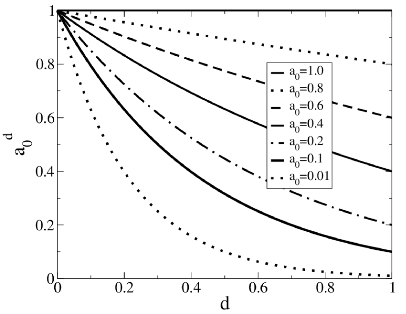
Figure 1: Plot of interaction strength ($a_{0}^{d}$) vs. metric distance between particles ($d$) within unit interaction radius for different distance dependent parameter ($a_{0}$=1,0.8,0.6,0.4,0.2,0.1,0.01) in decreasing order from top to bottom. For $a_{0}=1$ all the particles will interact with same interaction strength within unit interaction radius, as we decrease $a_{0}$ effective range of interaction decreases .

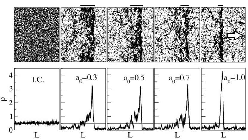
Figure 2: Upper panel : We plot real space snap shots of particle distribution. In the left most figure we plot initial condition for all distance dependent parameter ($a_{0}$). Other four plots are the real space particle distribution in steady state for $a_{0}=0.3,0.5,0.7,1.0$ from left to right. We draw a horizontal line in top of each real space snap shot which shows approximate length scale of the band and in right most figure we draw an arrow, which indicates the direction of movement of the band for all $a_{0}$. Lower panel : We plot density distribution ($\rho$) in horizontal direction or density distribution along the direction of band formation. Left most figure shows initial random density distribution for all $a_{0}$. Other four figures show density distribution for $a_{0}=0.3,0.5,0.7,1.0$ from left to right. In each figure we draw an horizontal line at $\rho=0.5$, mean density of the system. Here $\rho$ is the density along band direction and L is the system size. System parameters we have used, $L=256,\rho_{0}=0.5$ .

We numrically study the microscopic model introduced in Eqs.1 and 2 for different distance dependent interaction parameter $a_{0}$. Form of interaction potential is shown in Fig. 1 for different $a_{0}$ as a function of distance. For $a_{0}=1.0$, all the particles within the interaction radius interact with same strength, but as we decrease $a_{0}$ effective range of interaction decreases. We vary $a_{0}$ from $1.0$ to small value $0.01$ and for $a_{0}=0.0$ (no alignment interaction). We keep the speed $v_{0}=0.5$ of the particles. We start with initially homogeneous density and random orientation of the particles on a two dimensional lattice of size $L\times L$ and mean density $\rho_{0}$ with periodic boundary condition.
System shows a phase transition from disordered to long-ranged ordered state with the variation of noise strength $\eta$. Ordered state is characterised by global velocity defined by

$$V=|\frac{1}{N}\sum_{i=1}^{N}{\bf{n}}_{i}(t)|.$$ (8)

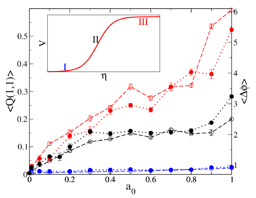
Typical plot of $V$ vs. $\eta$ is shown in cartoon picture in inset of Fig 6 We study our model in three different regions $I$(disordered), $II$ (close to transition:on the ordered side) and $III$ (deep ordered state) of phase diagram. First we study the model for region $II$ (close to transition). Since effective range of interaction as shown in Fig 1 decreases with $a_{0}$, hence for fixed density, critical value of noise strength also changes. For each $a_{0}=1.0,0.8,0.7,0.6,0.5,0.4,0.3,0.2,0.15,0.1,0.01$ we first estimate the critical $\eta_{c}(a_{0})$, then we choose value of $\eta(a_{0})=\eta_{c}-\delta\eta(a_{0})$, such that system have approximately same global velocity in the steady state. List of values of $\eta(a_{0})$ used in region $II$ of phase diagram is given in Table 1. We choose noise strength ($\eta$) in region $I$ and $III$, $0.7$ and $0.1$ respectively such that system is in the disordered/ordered state for all $a_{0}$.

Distance Dependent Interaction
Distance dependent parameter($a_{0}$)	Band density($\rho_{b}$)	Band width($W_{b}$)	Fraction of particle forming band ($n_{c}$)	Value of Noise-strength($\eta$) in region II
1	3.53	24	0.66	0.570
0.8	2.97	27	0.62	0.500
0.7	2.05	30	0.48	0.450
0.6	1.78	34	0.47	0.420
0.5	1.71	42	0.56	0.395
0.4	1.65	45	0.57	0.340
0.3	1.41	50	0.55	0.300
0.2	-	-	-	0.240
0.15	-	-	-	0.210
0.1	-	-	-	0.190
0.05	-	-	-	0.170
0.01	-	-	-	0.140

Table 1: Different numerical results for different distance dependent parameter ($a_{0}$). Here density within the band ($\rho_{b}$), which decreases with $a_{0}$ and width of the band ($W_{b}$), which increases as we decrease $a_{0}$. Also there is no clear band formation for $a_{0}<0.3$ that’s why we are not calculating $\rho_{b}$ and $W_{b}$ for $a_{0}<0.3$. Fraction of particles participating in band formation, that is almost same for all $a_{0}$ (47$\%$ to 66$\%$ particles are participating in band formation). We have also given $\eta$ values we have used to do all these calculation in region II of phase transition plot of global velocity in inset of Fig 6. System parameters we have used is same as Fig 2 .

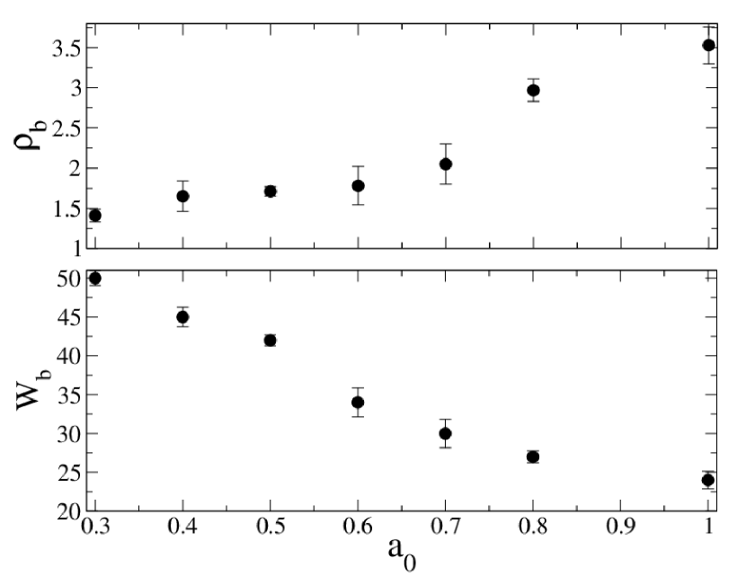
Figure 3: Upper panel : Plot of band density ($\rho_{b}$) vs. distance dependent parameter ($a_{0}$). $\rho_{b}$ increases as we increase $a_{0}$. Lower panel : We plot band width ($W_{b}$) vs. $a_{0}$ and $W_{b}$ increases as we decrease $a_{0}$. For $a_{0}<0.3$ there is no clear band formation. System parameters we have used is same as Fig 2 .

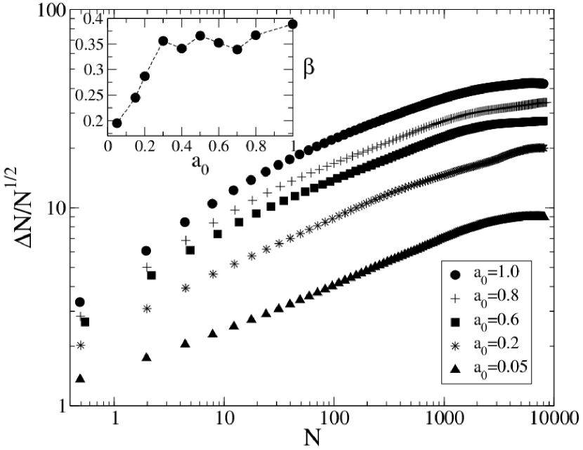
Figure 4: Plot of $\Delta N/N^{\frac{1}{2}}$ vs. N for different distance dependent parameter ($a_{0}$=1.0,0.8,0.6,0.2,0.05). In the inset we plot the exponent $\beta$ vs. $a_{0}$. For $a_{0}<0.3$, $\beta$ increases as we increase $a_{0}$, for $0.3<a_{0}<0.8$ there is a plateau region and for $a_{0}>0.8$ it increases again. For equilibrium system exponent $\beta=0.0$. System parameters we have used is same as Fig 2 .

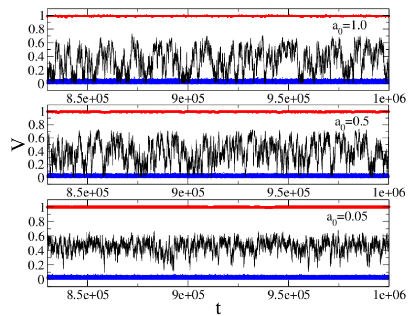
Figure 5: (Color online:) Plot of global velocity (V) vs. time for three different distance dependent parameter ($a_{0}=1.0,0.5,0.05$) in time span of $2\times 10^{5}$ from top to bottom in decrasing order. For each $a_{0}$ We choose three different region in phase transition plot of global velocity V , region I, region II and region III, are shown in inset of Fig 6. Here we are using different color for three different region, blue one for region I, black one for region II and red one for region III. System parameter we have used here, $L=50,\rho_{0}=1.0$ .

Figure 6: (Color online:) Plot of average density Phase separation order parameter along diagonal direction ($<Q(1,1)>$) and $<\Delta\phi>$ (defined in text) vs. distance dependent parameter ($a_{0}$) for three different region in global velocity V phase transition plot, are shown inset of Fig 6 , blue one for region I, black one for region II and red one for region III. In this figure left side we have labelled for $<Q(1,1)>$ and right side we have labelled for $<\Delta\phi>$ . We have used dotted line for $<Q(1,1)>$ and dashed line for $<\Delta\phi>$ plot. In both plot for smaller values of $a_{0}<0.3$ , $<Q(1,1)>$ and $<\Delta\phi>$ approches to zero, for $a_{0}>0.3$ and $a_{0}<0.8$ there is plateau region and for large value of $a_{0}>0.8$ to $a_{0}=1.0$ there is sharp increase in value of both $<Q(1,1)>$ and $<\Delta\phi>$. System parameters we have used here is same as Fig 2 .

IV Results

We first study our model in region $II$ of phase diagram: Each particle is chosen one by one and sequencially position and orientation are updated using Eqs. 1 and 2. Position and orientation of particles are stored in steady state, which we check by consistency of instantaneous global order parameter. Typical snapshot of particle’s position for four different values of $a_{0}=1.0,0.7,0.5,0.3$ at steady state and when there is clear band, is shown in Fig 2 (upper pannel). One of the main characteristic of polar flock, is the formation of bands in ordered state also obtained in previous study of Chate et al. chate2007 ,chate2008 . Similar bands are found in other microscopic models biplab as well as coarse-grained studies shradhapre . Our model reduces to the Vicsek’s type for $a_{0}=1.0$, where we also find clear bands as shown in Fig 2. As we vary $a_{0}$, size of the band increases as shown by increasing size of horizontal bar. Mean alignment of particles inside the band is perpendicular to the long axis of the band and bands typically move in one direction. Direction of motion of band is shown by big arrow in the Fig 2. In Fig 2 (lower panel), we plot the one dimensional distribution of density along the band direction and average over other direction. For $a_{0}=1.0$ density distribution shows sharp peak and width is small. As we decrease $a_{0}$, height of peak decreases and width increases. In Fig 3 we plot width of the band $W_{b}$, calculated from the width of the one dimensional density distribution, averaged over many snapshots. Mean density inside the band which we define as $\rho_{b}=\frac{N_{b}}{W_{b}\times L}$, where $N_{b}$ is the number of particles participate in band formation and $W_{b}$ is the width of the band. As shown in Fig 3 , mean density of particles inside the band increases as we increase $a_{0}$ and width of the band decreases with increasing $a_{0}$. In table 1 we show the variation of mean width of band $W_{b}$, mean density inside the band $\rho_{b}$ and fraction of particles participate for band formation $n_{c}=\frac{N_{b}}{N}$ for different distance dependent parameter $a_{0}$. We find although both $W_{b}$ and $\rho_{b}$ shows variation as we change $a_{0}$, but $n_{c}$ does not show any systematic change as we decrease $a_{0}$. It varies from $0.66$ (66 $\%$ particles) to $0.47$ (47 $\%$ particles). Also for $a_{0}<0.3$, there is no clear band formation, hence it is not possible to calculate different quantities (e.g $W_{b}$, $\rho_{b}$, etc.). Hence as we decrease $a_{0}$ system shows a change from high density narrow bands to low density wide bands and finally for very small $a_{0}$, there is no band.
Formation of high and low density bands should also be visible in two-point density structure factor. Finite size of bands or clusters show a presence of critical wavevector in the system. We calculate the two-point density structure factor $S({\bf q})$ using linearised calculation in ordered state. Details of calculation are given in appendix A. $S({\bf q})$ is calculated in the direction of ordering or along the bands direction. From Eqs.26 we find $S({\bf q})=\frac{v_{0}^{2}\rho_{0}^{2}\triangle_{0}}{c_{2}}[\frac{1}{q^{2}+q_{1}^{2}}+\frac{1}{q^{2}-q_{2}^{2}}]$ In the above expression of $S({\bf q})$, $c_{2}$ is a constant, is defined in 19 and expression for $q_{1}$ and $q_{2}$ is given in Eqs.27 and Eqs.28 respectively. $S({\bf q})$ diverges at critical wavevector $q_{c}=q_{2}=\sqrt{\frac{CB_{+}\alpha_{1}^{\prime}}{D_{V}v_{0}^{2}v_{1}^{2}}}$. Where $C=v_{0}V_{0}$ and $B_{+}$ is defined in Eqs. 29. Critical length scale $L_{c}=q_{c}^{-1}\simeq\sqrt{\frac{D_{V}v_{0}^{2}v_{1}^{2}}{CB_{+}\alpha_{1}^{\prime}}}$ decreases with increasing $\alpha_{1}^{\prime}=\frac{d\alpha}{d\rho}|_{\rho_{0}}$, which depends on the density dependence of $\alpha(\rho)$. For $\alpha_{1}^{\prime}=0$ or $\alpha$ is independent of density and Eqs. 6 reduces to Toner and Tu tonertu . Variation of width of the band $W_{b}$ in microscopic simulation with distance dependent parameter $a_{0}$ and dependence of critical wavevector $q_{c}$ with $\alpha_{1}^{\prime}$, shows one to one mapping between them.
Band formation in polar flock or clustering of particles also implies the density phase separation. In order to calculate density phase separation we first calculate fluctuation in density in cells of small size. To calculate such quantity, whole system is divided into $N_{c}$ small cells of size $1\times 1$. Hence for system of size $L\times L$, there will be $L^{2}$ small cells ($N_{c}=L^{2}$). We calculate number of particles in each cell in the steady state. Then standard deviation in particle number is calculated from different cells, which is defined by $\Delta\phi$

$$\Delta\phi=\sqrt{\frac{1}{N_{c}}\sum_{j=1}^{N_{c}}(\phi_{j})^{2}-(\frac{1}{N_{c}}\sum_{j=1}^{N_{c}}\phi_{j})^{2}}$$ (9)

where, $\phi_{j}$ is the number of particles in $j$th cell.

We also calculate Fourier transform of density defined by

$$Q({\bf k})=\mid\frac{1}{L}\sum_{i,j=1}^{L}e^{i{\bf k}\cdot{\bf r}}\rho(i,j)\mid$$ (10)

where ${\bf k}=\frac{2\pi(m,n)}{L}$, where $m,n$=$0$, $1$, $2$ …., $L-1$ are a two dimensional wave vector. We choose directions $(1,0)$ and $(0,1)$ as two directions of square box hence direction $(1,1)$ is along the diagonal of square box. During evolution of flock, direction of band changes with time. Hence to get maximum information about the clustering we calculate first non-zero value of $Q({\bf k})$ in the diagonal direction or $Q(1,1)$, where $m=n=1$. Both $\Delta\phi(t)$ and $Q(1,1)(t)$ are calculated at different times in the steady state. Then we average it over large time and calculate $<\Delta\phi>$ and $<Q(1,1)>$. Plot of $<\Delta\phi>$ and $<Q(1,1)>$ vs. $a_{0}$ is shown on right and left respectively of Fig. 6. $<\Delta\phi>$ and $<Q(1,1)>$ is calculated in all three regions of phase diagram (inset of Fig. 6). For region I in the phase diagram, where system is in the disordered state, both $<\Delta\phi>$ and $<Q(1,1)>$ remains small hence no phase separation. For region II or close to order-disorder transition, as we increase $a_{0}$, first both $\Delta\phi$ and $<Q(1,1)>$ increases with $a_{0}$, then shows a plateau type behaviour for $0.3<a_{0}<0.7$ and again increases for $a_{0}>0.7$. Hence system shows no phase separation for small $a_{0}$ and then gradually goes to moderate phase separation and finally for large $a_{0}$ shows strong phase separation. We find similar results for region III of phase diagram, where system is in the deep ordered state. Hence density shows another phase transition from phase separated to nonphase separated state as a function of distance dependent parameter $a_{0}$.

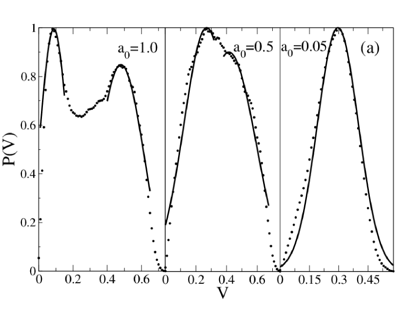
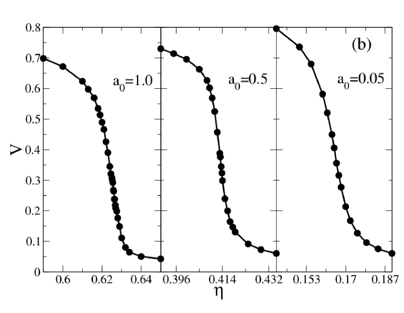
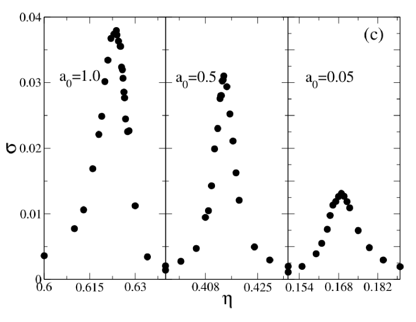
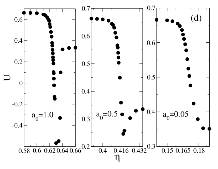
Figure 7: Upper panel: In figure (a) we plot probability distribution of Global velocity V for $a_{0}=1.0,0.5,0.05$ from left to right in decreasing order. Distribution of V changes bimodal to unimodal as we decrease $a_{0}$. In figure (b) we plot phase transition curve of V vs. noise strength $\eta$ in same order as in figure (a). Change in V becomes more and more sharp as we increase $a_{0}$. Lower panel: We plot variance ($\sigma$) of V vs. $\eta$ for $a_{0}=1.0,0.5,0.05$ from left to right in figure (c). $\sigma$ decays both side of critical noise strength $\eta_{c}$ for all $a_{0}$. In figure (d) we plot Binder cumulant (U) vs. $\eta$ in same order as in figure (c). For $a_{0}=1.0$ there is sharp jump in variation of U from ordered state ($U=2/3$) to disordered state ($U=1/3$), for $a_{0}=0.5$ jump in variation of U becomes less sharp and for $a_{0}=0.05$ variation of U becomes continuous from $U=2/3$ to $U=1/3$. System parameters we have used is same as Fig 5 .

We also calculate density fluctuation $\Delta N=\sqrt{<N^{2}>-<N>^{2}}$, as we vary distance dependent parameter $a_{0}$. We find for all $a_{0}$, density fluctuation $\Delta N/N^{1/2}\simeq N^{\beta}$ and $\beta>0.0$, hence density fluctuation is larger than thermal equilibrium system, where $\beta=0.0$. Large density fluctuation is one of the characteristic feature of active self-propelled systems chate2004 ; shradhaprl ; das2012 ; aditi . But we find the exponent $\beta$ varies as we tune $a_{0}$. In the inset of Fig 4, we plot variation of exponent $\beta$ for different $a_{0}$. $\beta$ vs. $a_{0}$ plot is almost flat with $\beta\simeq 0.4$ for $a_{0}>0.3$ and approaches zero for very small $a_{0}$.

Phase Transition : Now we characterise the order-disorder transition for three different values of distance dependent parameter $a_{0}=1.0$, $0.5$ and $0.05$. As shown in Fig 6 these three values of $a_{0}$ are three different points in density phase separation curve. For $a_{0}=1.0$, system is strongly phase separated, for $a_{0}=0.5$, moderate phase separation (plateau region) and for $a_{0}=0.05$, no phase separation. In Fig 5 we first plot the time series of global velocity for three different regions, region I, region II and region III as shown in inset of Fig 6. During a large span of time ($t=2\times 10^{5}$) in the steady state (after $t=8\times 10^{5}$), global velocity $V$ approches to value close to $1$ for all three $a_{0}$ in region $III$ and for region $I$ it approaches to $0$. But for region II system shows switching type behaviour, where system continuously switches from ordered $V\simeq 0.6$ to disordered $V\simeq 0.1$ state for $a_{0}=1$. Such switching behaviour of global velocity is also observed in previous study of chate2008 ,biplab ,shradhapre As we tune $a_{0}=0.5$, time series of global velocity shows weaker switching behaviour and for very small $a_{0}=0.05$ it shows huge fluctuation with no switching (shown in Fig 5). Probability distribution of global velocity $P({V})$ shows bistable behaviour for $a_{0}=1.0$ and gradually switches to unimodal behaviour for small $a_{0}$ as shown in Fig 7 (a). We have shown phase transition curve of V for three different $a_{0}$ in Fig 7 (b). For larger value of $a_{0}$ change in V with noise strength $\eta$ becomes very sharp and as we decrease $a_{0}$, change in V with $\eta$ becomes more and more continuous. We also calculate variance of order parameter $\sigma=\langle V^{2}\rangle-\langle V\rangle^{2}$, shown in Fig 7 (c) and also the fourth order binder cumulant defined by $U=1-\frac{<V^{4}>}{3<V^{2}>^{2}}$, Fig 7 (d) shows strong discontinuity from $1/3$ for disordered state to $2/3$ for ordered state as we approach critical $\eta$ for $a_{0}=1.0$ and discontinuity decreases with $a_{0}$ and smoothly goes from disordered value $1/3$ to ordered state value $2/3$ for $a_{0}=0.05$. System shows a transition from disordered to ordered state for all $a_{0}$, but nature of transition changes from first order type to continuous as we tune $a_{0}$. Also density changes from phase separated to nonphase separated state.

V Discussion

We studied a collection of polar self-propelled particles, interacting through distance dependent short range alignment interaction. Such distance dependent model is biologically motivated, where particles interact more strongly with their closest neighbours. Distance dependent interaction is introduced through an interaction parameter $a_{0}$, which varies from $1.0$ to $0.0$. For $a_{0}=1.0$, model reduces to Vicsek’s type and $a_{0}=0.0$, implies no interaction. For all $a_{0}$’s system shows a phase transition from disordered (global velocity $V=0.0$) to ordered (finite global velocity) as we vary noise intensity $\eta$. For large $a_{0}$ density shows formation of bands, characteristic of bands changes with $a_{0}$. For $a_{0}$ close to $1.0$, bands are strong with small width and high density and as we decrease $a_{0}$, bands become weak. Our numerical result is consistent with analytical calculation of density structure factor as shown in Eqs. 26. Where we find a critical wavevector at which structure factor diverges. The critical wave vector decreases or wavelength increases with decreasing $\alpha_{1}^{\prime}$.
Our finding in the work shows that density phase separation plays an important role in determining the nature of phase transition. First order phase transition in Vicsek’s model is because of strong density phase separation. Density phase separation in microscopic simulation can be tune in many ways, we can use distance dependent interaction, which controls the number of interacting neighbours. Changing the speed of particle in the Vicsek’s model will give the same result. For large speed system should show phase separated state and first order transition and for small speed we will have nonphase separated or continuous transition. Microscopic model we introduce here is not a unique distance dependent model, other models where interaction vary with other functional dependence on distance will also show the similar results.

Appendix A Linearised study of the broken symmetry state

The hydrodynamic equations Eqs.5 and 6, admit two homogeneous solutions: an isotropic state with ${\bf V}=0$ for $\rho<\rho_{c}$ and a homogeneous polarized state with ${\bf V}=V_{0}{\bf x}$ for $\rho>\rho_{c}$, where ${\bf x}$ is the direction of ordering. .We are mainly interested in the symmetry broken phase, specifically along the horizontal direction, in which direction large cluster or bands are moving. For $\alpha(\rho)>0$, We can write the polarization field as, ${\bf{V}}=(V_{o}+\delta V_{x}){\bf x}+\delta{\bf V}_{y}$, where ${\bf x}$ is the direction of band formation or horizontal direction and ${\bf y}$ is the perpendicular direction, $V_{0}{\bf x}=<{\bf{V}}>$ is the spontaneous average value of $\bf{V}$ in ordered phase. We choose $V_{0}=\sqrt{\frac{\alpha(\rho_{0})}{\beta}}$ and $\rho=\rho_{0}+\delta\rho$ where $\rho_{0}$, coarse-grained density. Combining the fluctuations we can write in a vector format,

$$\delta X_{\alpha}({\bf r},t)=\left[\begin{array}[]{c}\delta\rho\\ \delta V_{x}\\ \delta V_{y}\end{array}\right]$$ (11)

Now we introduce fluctuation in hydrodynamic equation for density then Eqs. 5 will reduce to,

$$\partial_{t}\delta\rho+v_{0}V_{0}\partial_{x}\delta\rho+v_{0}V_{0}\partial_{y}\delta\rho+v_{0}\rho_{0}\partial_{x}\delta_{V_{x}}+v_{0}\rho_{0}\partial_{y}\delta_{V_{y}}=0$$ (12)

Similarly we introduce fluctuation in velocity Eqs. 6, we are writing velocity fluctuation equations for horizontal direction or direction of band formation and for perpendicular direction. We are writing fluctuation equations for both direction separately, here x-is the direction of ordering and y is perpendicular direction. We have done Taylor series expansion of $\alpha(\rho)$ in Eqs.6 at $\rho=\rho_{0}$ and we have consider upto first order derivative term of $\alpha(\rho)$.

$$\partial_{t}{\delta{V_{x}}}=(\alpha(\rho_{0})+\alpha{{}_{1}^{\prime}}({\rho_{0}})\delta\rho)(V_{0}+\delta V_{x})-\beta(V_{0}^{2}+2V_{0}\delta V_{x})(V_{0}+\delta V_{x})-\frac{v_{1}}{2\rho_{0}}\partial_{x}\delta\rho+D_{V}\partial_{x}^{2}\delta V_{x}+D_{V}\partial_{y}^{2}\delta V_{x}-\lambda V_{0}\partial_{x}\delta V_{x}+{f_{Vx}}$$ (13)

$$\partial_{t}{\delta{V_{y}}}=(\alpha(\rho_{0})+\alpha{{}_{1}^{\prime}}({\rho_{0}})\delta\rho)(\delta V_{y})-\beta(V_{0}^{2}+2V_{0}\delta V_{x})(\delta V_{y})-\frac{v_{1}}{2\rho_{0}}\partial_{y}\delta\rho+D_{V}\partial_{x}^{2}\delta V_{y}+D_{V}\partial_{y}^{2}\delta V_{y}-\lambda V_{0}\partial_{x}\delta V_{y}+{f_{Vy}}$$ (14)

where $\alpha_{1}^{\prime}=\frac{\partial\alpha}{\partial\rho}\mid_{\rho_{0}}$ also $\lambda$ is combination of three $\lambda^{\prime}s(\lambda=\lambda_{1}+\lambda_{2}+2\lambda_{3})$ terms.
Now we are introducing Fourier component, $\delta\hat{\bf X}_{\alpha}({\bf k},t)=\int exp^{i({\bf k.r}-\omega t)}\delta X_{\alpha}({\bf r},t)$ in above three fluctuation equations 12, 13 and 14. Then the coupled equations we write in matrix form.

$$\left[\begin{array}[]{ccc}-i\omega+iv_{0}V_{0}q_{x}+iv_{0}V_{0}q_{y}&iv_{0}\rho_{0}q_{x}&iv_{0}\rho_{0}q_{y}\\ i\frac{v_{1}}{2\rho_{0}}q_{x}-\alpha{{}_{1}^{\prime}}(\rho_{0})V_{0}&-i\omega+2\alpha(\rho_{0})+D_{V}|q^{2}|+i\lambda V_{0}q_{x}&0\\ i\frac{v_{1}}{2\rho_{0}}q_{y}&0&-i\omega+2\alpha(\rho_{0})+D_{V}|q^{2}|+i\lambda V_{0}q_{x}\end{array}\right]\times\left[\begin{array}[]{c}\delta\rho\\ \delta V_{x}\\ \delta V_{y}\end{array}\right]=\left[\begin{array}[]{c}0\\ f_{Vx}\\ f_{Vy}\end{array}\right]$$ (15)

Earlier study shradhapre finds horizontal fluctuation or fluctuation in the direction of band formation is important when system is close to transition. Here in our numerical study we take region II, near to transition point, shown in the inset of Fig. 6. So, we are only considering fluctuation in ordering direction, then the above 3x3 matrix 15 reduce to,

$$\left[\begin{array}[]{cc}-i\omega+iv_{0}V_{0}q&iv_{0}\rho_{0}q\\ i\frac{v_{1}}{2\rho_{0}}q-\alpha{{}_{1}^{\prime}}(\rho_{0})V_{0}&-i\omega+2\alpha+D_{V}q^{2}+i\lambda V_{0}q\end{array}\right]\times\left[\begin{array}[]{c}\delta\rho\\ \delta V_{x}\end{array}\right]=\left[\begin{array}[]{c}0\\ f_{Vx}\end{array}\right]$$ (16)

We first determine the eigen frequencies of $\omega(\bf q)$ of these coupled equations and we find,

$$\omega_{\pm}=c_{\pm}q-i\varepsilon_{\pm}$$ (17)

where, the sound speeds,

$$c_{\pm}=\frac{1}{2}(\lambda+v_{0})V_{0}\pm c_{2}$$ (18)

with

$$c_{2}=\sqrt{(\frac{1}{4}(\lambda-v_{0})^{2}V_{0}^{2}+v_{0}v_{1})}$$ (19)

and the damping $\varepsilon_{\pm}$ in the Eqs. 17 are $O({\bf q^{2}})$ and given by,

$$\varepsilon_{\pm}=\pm\frac{c_{\pm}}{2c_{2}}[2\alpha+D_{V}q^{2}]\mp\frac{1}{2c_{2}}[2\alpha v_{0}V_{0}+v_{0}V_{0}\alpha_{1}^{\prime}+v_{0}V_{0}D_{V}q^{2}]$$ (20)

Here, important thing is that unlike isotropic problem $d>2$ there are no transverse mode, we always have just two longitudinal goldstone modes, associated with $\delta\rho$ and $V_{x}$.

Now the two-point density auto correlation along the direction of ordering,

$$\centering C_{\rho\rho}({\bf q},\omega)=\frac{v_{0}^{2}\rho_{0}^{2}2\triangle_{0}q^{2}}{(-\omega^{2}+(v_{0}+\lambda)V_{0}q\omega-v_{0}\lambda V_{0}^{2}q^{2}+\frac{v_{1}v_{0}q^{2}}{2})^{2}+[\omega(2\alpha+D_{V}q^{2})-q(2\alpha v_{0}V_{0}+v_{0}V_{0}\alpha_{1}^{\prime}+v_{0}V_{0}D_{V}q^{2})]^{2}}\@add@centering$$ (21)

$$\centering C_{\rho\rho}({\bf q},\omega)=\frac{v_{0}^{2}\rho_{0}^{2}2\triangle_{0}q^{2}}{(\omega-c_{+}q)^{2}(\omega-c_{-}q)^{2}+[\omega(2\alpha+D_{V}q^{2})-q(2\alpha v_{0}V_{0}+v_{0}V_{0}\alpha_{1}^{\prime}+v_{0}V_{0}D_{V}q^{2})]^{2}}\@add@centering$$ (22)

If we plot density-density correlation function as a function of $\omega$ there are two peaks at $\omega=c_{\pm}q$. From above density auto correlation it is very straight forward to calculate structure factor.

$$S(q,t)=\frac{1}{2\pi}\int_{-\infty}^{+\infty}\left\langle|\delta\rho(q,\omega)|^{2}\right\rangle d\omega=\frac{1}{2\pi}\int_{-\infty}^{+\infty}C_{\rho\rho}({\bf q},\omega)d\omega$$ (23)

$$S(q,t)=\frac{1}{2\pi}\int_{-\infty}^{+\infty}\frac{v_{0}^{2}\rho_{0}^{2}2\triangle_{0}q^{2}}{(\omega-c_{+}q)^{2}(\omega-c_{-}q)^{2}+[\omega(2\alpha+D_{V}q^{2})-q(2\alpha v_{0}V_{0}+v_{0}V_{0}\alpha_{1}^{\prime}+v_{0}V_{0}D_{V}q^{2})]^{2}}$$ (24)

$$S(q,t)=\frac{v_{0}^{2}\rho_{0}^{2}2\triangle_{0}q^{2}}{2c_{2}q}[\frac{1}{c_{+}q(2\alpha+D_{V}q^{2})-q(v_{0}V_{0}(2\alpha+D_{V}q^{2})+v_{0}V_{0}\rho_{0}\alpha_{1}^{\prime})}]$$ (25)

$$S(q,t)=\frac{v_{0}^{2}\rho_{0}^{2}\triangle_{0}}{c_{2}}[\frac{1}{q^{2}+q_{1}^{2}}+\frac{1}{q^{2}-q_{2}^{2}}]$$ (26)

where,

$$q_{1}^{2}=[\frac{v_{0}V_{0}\alpha_{1}^{\prime}B_{-}}{D_{V}v_{0}^{2}v_{1}^{2}}]$$ (27)

$$q_{2}^{2}=[\frac{v_{0}V_{0}\alpha_{1}^{\prime}B_{+}}{D_{V}v_{0}^{2}v_{1}^{2}}]$$ (28)

and

$$B_{\pm}=[\sqrt{\frac{1}{4}(\lambda-v_{0})^{2}V_{0}^{2}+v_{0}v_{1}}\mp\frac{1}{2}(\lambda-v_{0})V_{0}]$$ (29)

All the constants in wave vector expression is defined earlier. From there it is very clear $q_{1}^{2}$ and $q_{2}^{2}$ are positive. Now from above structure factor expression we get critical wave vector below which structure factor diverges,

$$D_{V}q_{2}^{2}=[\frac{v_{0}V_{0}\rho_{0}\alpha_{1}^{\prime}B_{+}}{v_{0}^{2}v_{1}^{2}}]-2\alpha B_{+}$$ (30)

When the system is near to critical point then $\alpha(\rho_{0})$ will be close to zero. Then we can write expression for critical wave vector,

$$q_{c}=q_{2}=\sqrt{\frac{CB_{+}\alpha_{1}^{\prime}}{D_{V}v_{0}^{2}v_{1}^{2}}}$$ (31)

Where, $C=v_{0}V_{0}$ Here for $\alpha_{1}^{\prime}\neq 0$ we get a critical wave vector $q_{c}$ at which structure factor diverges and it also gives a critical length scale $L_{c}$ of the system. Where, $\alpha_{1}^{\prime}$ is density dependent alignment term, which is similar to the distance dependence parameter $a_{0}$ in our numerical study and for $\alpha_{1}^{\prime}=0$ our study reduces to Toner and Tu study tonertu .

References

• (1) E. Ben-Jacob, I. Cohen, O. Shochet, A. CziroΒ΄Β΄π‘œ\acute{o}k and T. Vicsek, Phys. Rev. Lett. 75, 2899 (1995)
• (2) E. Rauch, M. Millonas and D. Chialvo, Phys. Lett. A 207, 185 (1995)
• (3) Physics Today 60, 28 (2007); C. Feare, The Starlings (Oxford: Oxford University Press) (1984)
• (4) S. Hubbard, P. Babak, S. Sigurdsson and K. Magnusson, Ecol. Model. 174, 359 (2004)
• (5) Toner, J., Y. Tu, and S. Ramaswamy, 2005, Ann. Phys. (Amsterdam) 318, 170
• (6) Ramaswamy, S., 2010, Annu. Rev. Condens. Matter Phys. 1, 323
• (7) M. Cristina Marchetti et al., Rev. Mod. Phys., 85, 1143, (2013).
• (8) E. Ben-Jacob, I. Cohen, O. Shochet, A. Tenenbaum, A. CzirΓ³k, and T. Vicsek, Phys. Rev. Lett. 75, 2899 (1995).
• (9) Hugues ChatΓ©, Francesco Ginelli, and Guillaume GrΓ©goire Phys. Rev. Lett. 99, 229601, (2007)
• (10) Hugues ChatΓ©, Francesco Ginelli, Guillaume GrΓ©goire, and Franck Raynaud Phys. Rev. E 77, 046113 (2008)
• (11) T.Β Vicsek et al., Phys.Β Rev.Β Lett. 75, 1226 (1995).
• (12) Francesco Ginelli and Hugues ChatΓ© ; Phys. Rev. Lett. 105, 168103 (2010) .
• (13) Anton Peshkov, Sandrine Ngo, Eric Bertin, Hugues ChatΓ©, and Francesco Ginelli ; Phys. Rev. Lett. 109, 098101
• (14) Biplab Bhattacherjee, Shradha Mishra, and S. S. Manna; Phys. Rev. E 92, 062134 (2015).
• (15) Andrea Cavagna, Lorenzo Del Castello, Supravat Dey, Irene Giardina, Stefania Melillo, Leonardo Parisi, and Massimiliano Viale; Phys. Rev. E 92, 012705 (2015).
• (16) J. Toner and Y. Tu, Phys. Rev. Lett. 75, 4326 (1995); Phys. Rev. E 58, 4828 (1998).
• (17) Shradha Mishra, Aparna Baskaran, and M. Cristina Marchetti Phys. Rev. E 81, 061916, (2010).
• (18) Guillaume GrΓ©goire and Hugues ChatΓ© ; Phys. Rev. Lett. 92, 025702 (2004).
• (19) Shradha Mishra and Sriram Ramaswamy ; Phys. Rev. Lett. 97, 090602 (2006).
• (20) Dipjyoti Das, Dibyendu Das , Ashok Prasad ; Journal of Theoretical Biology 308 (2012) 96–104.
• (21) S. Ramaswamy, R. Aditi Simha and J. Toner ; EPL (Europhysics Letters) 62, 196 (2003)