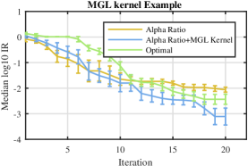
Advancing Bayesian Optimization: The Mixed-Global-Local (MGL) Kernel and Length-Scale Cool Down
Kim Peter Wabersich Marc Toussaint
Machine Learning and Robotics Lab, University of Stuttgart Machine Learning and Robotics Lab, University of Stuttgart
Abstract
Bayesian Optimization (BO) has become a core method for solving expensive black-box optimization problems. While much research focussed on the choice of the acquisition function, we focus on online length-scale adaption and the choice of kernel function. Instead of choosing hyperparameters in view of maximum likelihood on past data, we propose to use the acquisition function to decide on hyperparameter adaptation more robustly and in view of the future optimization progress. Further, we propose a particular kernel function that includes non-stationarity and local anisotropy and thereby implicitly integrates the efficiency of local convex optimization with global Bayesian optimization. Comparisons to state-of-the art BO methods underline the efficiency of these mechanisms on global optimization benchmarks.
1 INTRODUCTION
Bayesian Optimzation (BO) became an almost ubiquitous tool for general black-box optimization with high function evaluation cost. The key idea is to make use of the gathered data by computing the Bayesian posterior over the objective function. A BO algorithm is in principle characterized by two choices: 1) What is the prior over the objective function? 2) Given a posterior, what is the decision theoretic criterion, the so-called acquisition function, to choose the next query point?
Previous research has extensively focussed on the second question. For instance, recent work goes beyond Expected Improvement (Jones, 2001) and UCB (Srinivas et al., 2012) by proposing the entropy of the optimum location (Hernández-Lobato et al., 2014) or an infinite metric based criterion (Kawaguchi et al., 2015) as acquisition function.
In this paper we rather focus on the first question, the choice of model or prior over the objective function. Clearly, from the purely Bayesian stance the prior must be given and is not subject to discussion. However, there are a number of reasons to reconsider this:
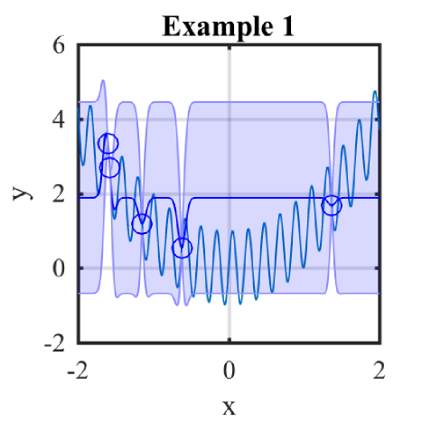
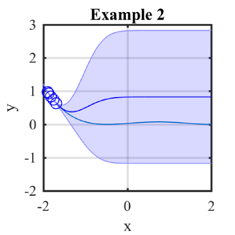
Choice of Hyperparameters: A large number of methods, notably with the exception of Hernández-Lobato et al. (2014), rely on an online point estimate of the hyperparameters. Many convergence proofs in fact rely on an apriori chosen GP hyperprior (see also Tab. 1 for details). Several experimental results are reported where hyperpriors have been carefully chosen by hand or optimized on samples from the objective function which are apriori not given (Srinivas et al., 2012; Wang et al., 2014; Kawaguchi et al., 2015). In practise, choosing the hyperprior online (e.g. using leave-one-out cross-validation (LOO-CV) on the so-far seen data) is prone to local optima and may lead to significant inefficiency w.r.t. the optimization process. For instance, in Fig. 1(a) we see that with a maximum likelihood estimate of the length-scale we may get an unuseful view of the objective function. Taken together, we believe that online selection of hyperparameters during online learning remains a key challenge.
In this paper we take the stance that if one chooses a point estimate for the hyperprior online, then maximum likelihood only on the seen data is not an appropriate model selection criterion. Instead, we should choose the hyperprior so as to accelerate the optimization process. We propose to cool down a length-scale parameter based on hyperprior selection w.r.t. the acquisition function, that is, which hyperprior promises more “acquisition” with the next query point. We combine this with a lower-bound heuristic for robustness.
Choice of kernel function: The squared-exponential kernel is the standard choice of prior. However, this is in fact a rather strong prior as many relevant functions are heteroscedastic (have different length-scales in different regions) and have various local optima, each with different non-isotropic conditioning of the Hessian at the local optimum. Only very few preliminary experiments on heteroscedastic and non-isotropic models have been reported (Martinez-Cantin, 2015; Mohammadi et al., 2016).
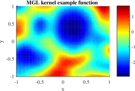
In this paper we propose a novel type of kernel function with the following in mind. Classical model-based optimization of convex black-box functions (Nocedal and Wright, 2006, Section 8) is extremely efficient iff we know the function to be convex. Therefore, for the purpose of optimization we may presume that the objective function has local convex polynomial regions, that is, regions in which the objective function is convex and can reasonably be approximated with a (non-isotropic) 2nd-order polynomial, such that within these regions, quasi-Newton type methods converge very efficiently. Like it would be the case in Fig 1(b). To this effect we propose the Mixed-Global-Local (MGL) kernel, which expresses the prior assumption about local convex polynomial regions, as well as automatically implying a local search strategy that is analogous to local model-based optimization. Effectively, this choice of kernel integrates the efficiency of local model-based optimization within the Bayesian optimization framework.
In summary, our contributions are
-
•
An online hyperparameter cool down method based on the acquisition function instead of maximum likelihood, which we call alpha-ratio cool down, and a length-scale lower bound for robustness.
-
•
A novel kernel function to represent local convex polynomial regions, that implies local quadratic interpolation and optimization steps analogous to classical (quasi-Newton-type) model-based optimization combined with global Bayesian optimization.
-
•
An efficient algorithm for detecting local convex polynomial regions.
Our paper is structured as follows: After giving the essential BO background, we explain a length-scale cool down scheme for isotropic kernels. Next we introduce the MGL kernel which will make use of the adaption scheme from the first step. In the end we will show significant performance improvements compared to classical BO with ’optimal’ (see Rem. 4) hyperparameters.
1.1 Problem Statement and Bayesian optimization background
We consider the black-box optimization problem
| (1) |
with an objective that maps a hypercube
| (2) |
to real numbers. We consider a Gaussian process (GP) (Rasmussen, 2006) prior over with constant prior mean function . Together with a covariance (kernel) function we write for the prior GP in short. Given samples at points where , the posterior GP reads
| (3) | ||||
| (4) | ||||
| (5) |
, is the posterior covariance, is the positive definite kernel or matrix and the prior mean, stacked in a vector. A very common choice of kernel is the squared exponential (SE) kernel
| (6) |
with hyperparameters (length-scale) and (prior variance). The GP model assumption about builds the basis for many BO algorithms. A general prototype for such an algorithm is given in Alg. 1, where represents the algorithm specific acquisition function. For experiments we will use the well known and theoretical extensively studied Expected Improvement (EI) (Bull, 2011) acquisition function, which is defined as
| (7) |
with and .
| ACQUISITION FCN | T | A |
|---|---|---|
| Expected Improvement (EI) | ✓ | ✓ |
| (Bull, 2011) | ||
| Upper Confidence Bound (UCB) | ✓ | ✗ |
| (Srinivas et al., 2012) | ||
| Entropy Search (PES) | ✗ | ✗ |
| (Hernández-Lobato et al., 2014) | ||
| Exponential Convergence | ✓ | ✗ |
| (Kawaguchi et al., 2015) |
1.2 Related work
Classical online model adaption in BO through maximum likelihood or LOO-CV (Rasmussen, 2006) are compared in Bachoc (2013). LOO-CV turns out to be more robust under model misspecification whereas maximum likelihood gains better results as long as the model is chosen ’well’. Jones (2001) already discusses the problem of highly misleading initial objective function samples. In Forrester and Jones (2008) an idea earlier mentioned in Jones (2001) is studied, where the hyperparameter adaption is combined with the EI calculation in one step. The authors show better performance in certain cases, while the resulting sub-optimization can get quite tedious as described in Quttineh and Holmström (2009). Another approach for improving the length-scale hyperparameter adaption is presented in Wang et al. (2016). They try to limit local exploration by setting an upper bound on the length-scale. The bound they propose is independent of dimensionality and experimentally chosen by hand for their applications. Those papers address the same problem but all of them are modifications of the basic approach to adjust hyperparameters to maximize data likelihood. In contrast we adjust hyperparameters based on the aquisition function, aiming at optimization performance rather than data likelihood.
Mohammadi et al. (2016) introduce the idea of local length-scale adaption based on maximizing the acquisition function (EI) value, which is not efficient as they say (and different to the cool down we propose). Nevertheless we endorse the underlying idea, since it is related to our motivation.
On the model side there are several ideas which yield non-isotropic models by building an ensemble of local isotropic kernels, e.g. based on trees (Assael et al., 2014). We however introduce a specific kernel rather than a concept of combining kernels or Gaussian processes taylored for improving BO.
There are also concepts regarding locally defined kernels, e.g. Krause and Guestrin (2007). The idea of Martinez-Cantin (2015) is somehow closely related to ours, because they use a local and a global kernel function, which is a great approach, as we believe. They parametrize the location of the local kernel as well as the respective parameters. Consequently they end up with a large number of hyperparameters which makes model selection very difficult. In constrast to their work we are able to gain comparable or better performance in well-known benchmarks. At the same time we overcome the problem of many hyperparameters by a separated, efficient algorithm for determining the location of local minimum regions. Furthermore we use a non-isotropic kernel for better fitting local minimum regions.
As a last aspect we want to mention, that PES, (Hernández-Lobato et al., 2014) also incorporates a local minimum region criterion encapsulated in the acquisition function itself, what we find is very interesting and is conceptually connected to our ideas. We compare the performance of PES along with another state-of-the-art BO algorithm (Kawaguchi et al., 2015) against our advances in combination with classical EI in the experimental section.
2 LENGTH-SCALE COOL DOWN
In this section we address length-scale adjustment of an isotropic kernel during the optimization process as part of the general BO Algorithm (Alg. 1, Line 6). Most commonly, at iteration is chosen such that the model represents the observed data well. This approach however ignores the closed loop, i.e., that the next sample choice will depend on . In contrast we aim to control the optimization process characteristics by performing a transition from “macro” to “micro” modelling of the objective function.
2.1 Alpha-ratio cool down
Let be the length-scale used in the previous iteration. In our approach we want to decide whether to reuse the same length-scale or decrease it to a specific smaller length-scale in iteration . In our experiments we will choose , where is a hard lower bound we present in the next section. Neglecting this bound, we want to decide whether to half the length-scale.
We propose to use the aquisition function as a criterion for this decision. Let
| (8) |
be the alpha-ratio, where is the optimal aquisition value when using length-scale . In typical situations we expect that because the reduced length-scale leads to larger posterior variance, which typically leads to larger aquisition values, i.e., more chances for progress in the optimization process. We turn this argument around: if is not substantially larger than 1, then choosing the smaller length-scale does not yield substantially more chances for progress in the optimization process. In this case, as a smaller length-scale has higher risk of overfitting (Fig. 1(a)), we decide to stick to the old length-scale .
In summary, in our alpha-ratio (AR) cool down for length-scale adaption we have a fixed threshold and choose as new length-scale if , and otherwise. In Alg. 2 we summarize the scheme, where in lines 2-5 the calculation of the alpha-ratio is shown.
Remark 1.
It is straight-forward to transfer existing convergence guarantees of Bayesian Optimization, as given in Bull (2011), to hold also in the case of AR cool down by a constant absolute lower bound , such that we have
| (9) |
throughout the optimization.
2.2 Lower Bound on Correlation
To increase the robustness of length-scale adaptation especially in the very early phase of optimization we propose a length-scale lower bound that explicitly takes the search space dimensionality into account. To find such a lower bound, we assume that we have an idea about minimum correlation that two points should have at all time. For constructing the lower bound on length-scale we consider the following best case regarding the correlation: The samples are chosen in a way, such that the minimal correlation of any new point with the data is highest. Based on for different number of samples , we calculate the corresponding minimum length-scale to satisfy the minimum required correlation . Since it is very likely, that samples acquired by Alg. 1 will violate the best case assumption, the calculated length-scale serves as a lower bound. Formally consider the set
| (10) |
and (for the design scheme) which yields highest correlation values for an “adversarial” . Note that in is not relevant for (10). Even if an acquisition function will not explore the search space in terms of (10) we at least want to guarantee that in case of (10) we would have a minimum correlation. To this end we solve
| (11) |
for , which is the length-scale lower bound we are searching for.
Remark 2.
2.2.1 Approximation for higher dimensions
Now we use the 1D result (Rem. 2) with the following idea in order to transfer the bound to higher dimensions: The max. distance in 1D between samples implies a minimal, empty (sample free) space. We demand that in higher dimensions the ratio between the volume of the whole search space () and this minimal empty space remains the same. Thereby we seek to get equal coverage of every sample in case . Following this idea, we transform the minimum distance
| (13) |
for (, compare with Rem. 2) in terms of the sphere volume
| (14) |
(Weisstein, 2016), to obtain a reasonable approximation for higher dimensions . I.e. given we calculate and solve
| (15) |
for which allows us together with as in (11) to obtain the corresponding length-scale lower bound. By applying these steps using the example of the SE kernel (6) we get
| (16) |
as lower bound for the length-scale by setting .
3 MIXED-GLOBAL-LOCAL KERNEL
In this section we introduce the MGL kernel. We assume that each local (global) optimum of (1) is within a neighbourhood that can be approximated by a positive definite quadratic function. More precisely:
Definition 1.
Given a data set , we call a convex subset a convex neighborhood if the solution of the regression problem
| (17) |
( the data points in ) has a positive definite Hessian .
If we are given a set of convex neighborhoods that are pair-wise disjoint we define the following kernel function:
Definition 2.
The Mixed-Global-Local (MGL) kernel is given by
| (18) |
for any ,
where is a stationary-isotropic kernel (Rasmussen, 2006)
and
| (19) |
the quadratic kernel.
This kernel is heteroscedastic in the sense that the quadratic kernels in the convex neighborhood implies fully different variances than the “global” stationary-isotropic kernel around the neighborhoods. Due to the strict seperation of the corresponding regions, the posterior calculation can be decoupled.
3.1 MGL kernel hyperparameter adaption
The hyperparameters of the MGL kernel are the length-scale and other parameters (prior mean , prior variance ) of the isotropic kernel and the convex neighborhoods . For the model update in Alg. 1, line 6 we have to update these hyperparameters. For the length-scale we use Alg. 2 and adapt the remaining parameters with maximum likelihood or LOO-CV. For determining we introduce Alg. 3. The main simplification is the discretization of the search space using the samples as centers for k-nearest-neighbor (kNN) search. As soon as a kNN tuple of samples satisfy Def. 1, we get a ball shaped local minimum region. In line 6,7 we calculate a potential local minimum region. In line 8 we fit a quadratic form using the samples inside this region. Lines 9-27 are used as selection criterion for local regions. Besides trivial criterions, in line 21 we add a local convergence criteria. In line 25 we force close points to the local region to contribute to the local model which turned out to improve overall performance. Line 31 removes all regions that overlap with better regions in order to find a disjoint set of convex neighborhoods.
Remark 3.
4 EMPIRICAL RESULTS
We first give some illustrative examples of the behavior of the alpha-ratio cool down and the MGL kernel, before comparing quantitatively the performance against other methods on benchmark problems.
The original source code which was used to generate all of the results can be found in the supplementary material and will be published. For all tests we choose the following configurations: For Alg. 2 we set , and for Alg. 3 we choose . For the MGL-kernel (18) we take the SE kernel (6) for . We estimated the observation variance in (6) and the constant mean of the prior GP via maximum likelihood and scaled the observation variance down by factor for consistency with the quadratic part of (18) if any local region is detected. For computing Alg. 1 line 7 we first solved the minimization using the kernel of (18) and compared it with the results of the minimization problems using the kernel for each local minimum region since all the regions for the different kernel parts are disjoint. We used three samples as initial design set, chosen by latin hypercube sampling.
Remark 4.
In the following we will often refer to an optimal choice of hyperparameters. By this we mean that 1000 random samples from the respective objective function are taken. On this data an exhaustive LOO-CV is used to select the length-scale, and max-likelihood to select the prior variance and mean-prior .
4.1 Illustrating the AR cool down
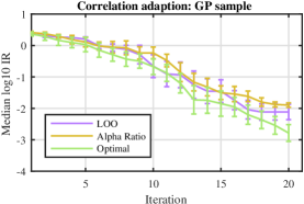
To illustrate AR cool down (Alg. 2) within Bayesian Optimization (Alg. 1) we consider the ideal setting where the objective is sampled from a GP with a stationary SE kernel. In Fig. 2(a) we display the regret when using 1) the optimal parameters (Rem. 4), 2) online
an exhaustive LOO-CV for length-scale parameter and and estimated from data using maximum likelihood, and 3) our AR cool down method. As the true objective is indeed a sample from a stationary isotropic GP, online LOO-CV and optimal hyperparameters work well, while AR cool down has less variance in performance. belfig:ExamplesMINkernel
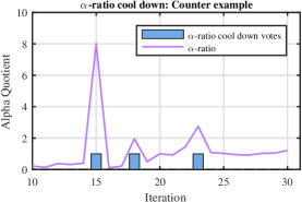
To give more insight, in Fig. 2(d) the mechanics of Alg. 2 are illustrated. Shown is the alpha-ratio (8) and the cool down events are indicated by the small bars.
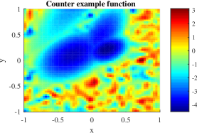
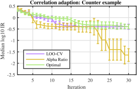
Finally, we illustrate AR cool down in case of the non-stationary heteroscedastic objective function given in Fig. 2(b). Note its structure mixing small and large length-scale local optima. The regret curves in Fig. 2(c) compare the same three methods described above. Both, the optimal and online LOO-CV methods try to fit stationary GP hyperparameters to a heteroscedastic objective function. Both of these lead to rather poor optimization behavior. AR cool down behaviors clearly superior.
4.2 Illustrating the MGL kernel
4.3 Comparision with PES, IMGPO and EI
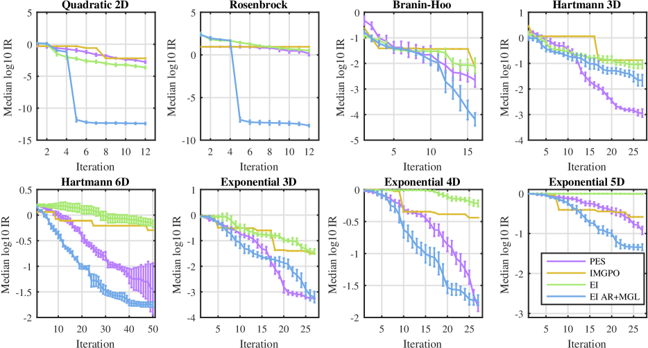
In Fig. 3 we report on results using several synthetic benchmark functions. Shown are predictive entropy search (PES) (Hernández-Lobato et al., 2014) (which treats hyperparameters in a Bayesian way in the acquisition function), infinite metric GP optimization (IMGPO) (which uses a Bayesian update for hyperparameters in each iteration), classical EI with optimal (Rem. 4) hyperparameters, and EI using our alpha-ratio model adaption and the MGL-kernel (EI AR + MGL).
For all performance tests where we show the log10 median performance, we made 32 runs and estimated the median variance via bootstrapping. The errorbars indicate one times the standard deviation.
The results of PES111https://github.com/HIPS/Spearmint/tree/PESC and IMGPO222http://lis.csail.mit.edu/code/imgpo.html search are obtained using the code available online. Therefore the results are somehow biased through the prior on the hyperparameters in these algorithms.
In addition to commonly considered benchmark functions (Rosenbrock, Branin-Hoo, Hartmann3D, Hartmann 6D) taken from Surjanovic and Bingham (2016), we show a simple quadratic function in the interval and an exponential function of the form with on the same interval in respective dimensions .
The MGL-kernel outperforms significantly in case of the quadratic and the more quadratic like Rosenbrock objective. Also for Branin-Hoo, Hartmann 6D and Exponential 5D our method significantly outperforms existing state-of-the-art Bayesian optimization methods. In case of Hartmann 3D, PES turns out to work better. Nevertheless we want to emphasize the outstanding improvement compared to plain EI with optimal (Rem. 4) hyperparameters in every test case.
5 CONCLUSION
Both of our core contributions, length-scale cool down based on the acquisition function, and the MGL kernel function, concern model selection. From a higher-level perspective we proposed that in the context of Bayesian Optimization we should select models differently than in standard Machine Learning: Instead of selecting hyperparameters based on maximum likelihood on the previous data we should try to judge the implications of the choice of hyperparameter on the future data, e.g., via the acquisition function. And instead of choosing a standard “uninformed” squared exponential kernel we may want to choose a kernel function that indirectly expresses our prior that model-based optimization is efficient in local convex (non-isotropic) regions, while the global length-scale characterizes where further local regions may are hidden.
We found that our novel concept of length-scale adpation outperforms leave-one-out cross validation and even a-posteriori optimal hyperparameters in the robust setting and has similar performance in the nominal case.
Further, combining length-scale cool down and our novel MGL kernel function with Expected Improvement shows in most benchmark problems better performance while no assumptions on the model hyperparameters were made beforehand. Furthermore we are not limited to EI which enables the community to combine the length-scale adaption and model with other acquisition functions, which potentially will lead to an overall performance improvement regarding Bayesian optimization as we believe.
References
References
- Assael et al. (2014) John-Alexander M Assael, Ziyu Wang, Bobak Shahriari, and Nando de Freitas. Heteroscedastic treed bayesian optimisation. arXiv preprint arXiv:1410.7172, 2014.
- Bachoc (2013) François Bachoc. Cross validation and maximum likelihood estimations of hyper-parameters of gaussian processes with model misspecification. Computational Statistics & Data Analysis, 66:55–69, 2013.
- Bull (2011) Adam D Bull. Convergence rates of efficient global optimization algorithms. Journal of Machine Learning Research, 12(Oct):2879–2904, 2011.
- Forrester and Jones (2008) Alexander IJ Forrester and Donald R Jones. Global optimization of deceptive functions with sparse sampling. In 12th AIAA/ISSMO multidisciplinary analysis and optimization conference, volume 1012, 2008.
- Hernández-Lobato et al. (2014) José Miguel Hernández-Lobato, Matthew W Hoffman, and Zoubin Ghahramani. Predictive entropy search for efficient global optimization of black-box functions. In Advances in neural information processing systems, pages 918–926, 2014.
- Jones (2001) Donald R Jones. A taxonomy of global optimization methods based on response surfaces. Journal of global optimization, 21(4):345–383, 2001.
- Kawaguchi et al. (2015) Kenji Kawaguchi, Leslie Pack Kaelbling, and Tomás Lozano-Pérez. Bayesian optimization with exponential convergence. In Advances in Neural Information Processing Systems, pages 2809–2817, 2015.
- Krause and Guestrin (2007) Andreas Krause and Carlos Guestrin. Nonmyopic active learning of gaussian processes: an exploration-exploitation approach. In Proceedings of the 24th international conference on Machine learning, pages 449–456. ACM, 2007.
- Martinez-Cantin (2015) Ruben Martinez-Cantin. Locally-biased Bayesian optimization using nonstationary Gaussian processes. In Neural Information Processing Systems (NIPS) workshop on Bayesian Optimization, 2015.
- Mohammadi et al. (2016) Hossein Mohammadi, Rodolphe Le Riche, and Eric Touboul. Small ensembles of kriging models for optimization. arXiv preprint arXiv:1603.02638, 2016.
- Nocedal and Wright (2006) Jorge Nocedal and Stephen Wright. Numerical optimization. Springer Science & Business Media, 2006.
- Quttineh and Holmström (2009) Nils-Hassan Quttineh and Kenneth Holmström. Implementation of a one-stage efficient global optimization (ego) algorithm. 2009.
- Rasmussen (2006) Carl Edward Rasmussen. Gaussian processes for machine learning. 2006.
- Srinivas et al. (2012) Niranjan Srinivas, Andreas Krause, Sham M Kakade, and Matthias W Seeger. Information-theoretic regret bounds for gaussian process optimization in the bandit setting. IEEE Transactions on Information Theory, 58(5):3250–3265, 2012.
- Surjanovic and Bingham (2016) S. Surjanovic and D. Bingham. Virtual library of simulation experiments: Test functions and datasets. Retrieved September 21, 2016, from http://www.sfu.ca/ ssurjano, 2016.
- Wang et al. (2014) Ziyu Wang, Babak Shakibi, Lin Jin, and Nando de Freitas. Bayesian multi-scale optimistic optimization. In AISTATS, pages 1005–1014, 2014.
- Wang et al. (2016) Ziyu Wang, Frank Hutter, Masrour Zoghi, David Matheson, and Nando de Feitas. Bayesian optimization in a billion dimensions via random embeddings. Journal of Artificial Intelligence Research, 55:361–387, 2016.
- Weisstein (2016) Eric W. Weisstein. Hypersphere. From MathWorld—A Wolfram Web Resource, 2016. URL http://mathworld.wolfram.com/Tree.html. Last visited on 13/4/2012.
