Precision neutrino experiments vs the Littlest Seesaw

Abstract

We study to what extent upcoming precision neutrino oscillation experiments will be able to exclude one of the most predictive models of neutrino mass and mixing: the Littlest Seesaw. We show that this model provides a good fit to current data, predicting eight observables from two input parameters, and provide new assessments of its predictions and their correlations. We then assess the ability to exclude this model using simulations of upcoming neutrino oscillation experiments including the medium-distance reactor experiments JUNO and RENO-50 and the long-baseline accelerator experiments DUNE and T2HK. We find that an accurate determination of the currently least well measured parameters, namely the atmospheric and solar angles and the CP phase $\delta$, provide crucial independent tests of the model. For $\theta_{13}$ and the two mass-squared differences, however, the model’s exclusion requires a combination of measurements coming from a varied experimental programme. Our results show that the synergy and complementarity of future experiments will play a vital role in efficiently discriminating between predictive models of neutrino flavour, and hence, towards advancing our understanding of neutrino oscillations in the context of the flavour puzzle of the Standard Model.

1 Introduction

The framework of neutrino masses and mixing for explaining neutrino oscillations — the first direct experimental evidence for physics beyond the Standard Model — is now firmly established nobel . All three mixing angles together with the size of the two mass-squared differences have been measured, with experimental efforts now focused on determining the final few unknowns: the ordering and scale of the neutrino masses; the value of the Dirac phase $\delta$; and a precision measurement of the angle $\theta_{23}$ including, if non-maximal, its octant. Although there is some as yet inconclusive evidence for $\delta$ in the third or fourth quadrant, as well as for normal ordering (NO) and non-maximal atmospheric mixing, we rely on the next generation of oscillation experiments to set these issues to rest.

On the theoretical side, however, the origin of neutrino masses and mixing remains unknown with many possible models considered viable (for reviews see e.g. King:2013eh ; King:2015aea ). A large proportion of these models are based on the classic seesaw mechanism, involving heavy right-handed Majorana neutrinos seesaw , providing both a mechanism for generating the neutrino masses and a natural explanation for their smallness. However, in order to make predictions that can be probed experimentally, seesaw models require additional assumptions or constraints King:2015sfk .

To accommodate the three distinct light neutrino masses which drive the oscillation phenomenon, the seesaw mechanism requires at least two right-handed neutrinos King:1999mb . In order to reduce the number of free parameters still further to the smallest number possible, and hence increase predictivity, various approaches to the two right-handed neutrino seesaw model have been suggested, such as postulating one King:2002nf or two Frampton:2002qc texture zeroes in the Dirac mass matrix in the flavour basis (i.e. the basis of diagonal charged lepton and right-handed neutrino masses). However, such two texture zero models are now phenomenologically excluded Harigaya:2012bw for the case of a normal neutrino mass hierarchy. The minimal two right-handed neutrino model with normal hierarchy which can accommodate the known data of neutrino mixing involves a Dirac mass matrix with one texture zero and a characteristic form known as the Littlest Seesaw model King:2013iva . The Littlest Seesaw model may be embedded in unified models of quarks and leptons in Bjorkeroth:2015ora . It leads to successful leptogenesis where the sign of baryon asymmetry is determined by the ordering of the heavy right-handed neutrinos, and the only seesaw phase $\eta$ is identified as the leptogenesis phase, linking violation of charge parity symmetry (CP) in the laboratory with that in the early universe Bjorkeroth:2015tsa .

The Littlest Seesaw model can be understood as an example of sequential dominance (SD) King:1998jw in which one right-handed neutrino provides the dominant contribution to the atmospheric neutrino mass, leading to approximately maximal atmospheric mixing, while the other right-handed neutrino gives the solar neutrino mass and controls the solar and reactor mixing as well as the magnitude of CP violating effects via $\delta$. SD generally leads to normal ordering and a reactor angle which is bounded by $\theta_{13}\lesssim m_{2}/m_{3}$ King:2002nf , proposed a decade before the reactor angle was measured nobel . Precise predictions for the reactor (and solar) angles result from applying further constraints to the Dirac mass matrix, an approach known as constrained sequential dominance (CSD) King:2005bj . For example, keeping the first column of the Dirac mass matrix proportional to $(0,1,1)^{T}$, a class of CSD($n$) models has emerged King:2005bj ; Antusch:2011ic ; King:2013iva ; King:2013xba ; Bjorkeroth:2014vha corresponding to the second column proportional to $(1,n,(n-2))^{T}$, with a reactor angle approximately given by King:2015dvf $\theta_{13}\sim(n-1)\frac{\sqrt{2}}{3}\frac{m_{2}}{m_{3}}$. The Littlest Seesaw model corresponds to $n=3$ with a fixed seesaw phase $\eta=2\pi/3$.

It was recently realised that the alternative form of the Littlest Seesaw model with second column $(1,1,3)^{T}$ and seesaw phase $\eta=-2\pi/3$ (also proposed in King:2013iva ) may be enforced by an $S_{4}\times U(1)$ symmetry, putting this version of the Littlest Seesaw model on a firm theoretical foundation King:2016yvg in which the required vacuum alignment emerges from symmetry as a semi-direct model King:2009ap . In general the Littlest Seesaw model is an example of trimaximal TM₁ mixing Xing:2006ms ; Albright:2008rp , in which the first column of the tri-bimaximal mixing matrix Harrison:2002er is preserved, similar to the semi-direct model of trimaximal TM₁ mixing that was developed in Luhn:2013vna . To fix the seesaw phase, one imposes a CP symmetry in the original theory which is spontaneously broken, where, unlike Ding:2013hpa , there is no residual CP symmetry in either the charged lepton or neutrino sectors, but instead the phase $\eta$ in the neutrino mass matrix is fixed to be one of the cube roots of unity due to a $Z_{3}$ family symmetry, using the mechanism proposed in Antusch:2011sx .

As explained in more detail later on, the Littlest Seesaw model predicts all neutrino masses and mixing parameters in terms of two or three parameters, and it has been shown that the model is in agreement with all existing data, for a suitable range of its internal parameters Bjorkeroth:2014vha . The model makes some key predictions about the neutrino mass spectrum, that the lightest neutrino is massless $m_{1}=0$ and that normal ordering obtains $\Delta m^{2}_{31}>0$, which offer a means to exclude it via the observation of neutrinoless double beta decay, the measurement of the beta-decay end-point, or from cosmological measurements, as well as any measurement of NO from neutrino oscillation searches. However, it also provides a rich set of predictions and correlations for the mixing angles and phases. In this paper, we assume Normal Hierarchy ($m_{1}=0$ and NO), and study how the future long- and medium-baseline oscillation programme will be able to test this model through the precision measurement of the oscillation parameters.

The layout of the paper is as follows: in Section 2 we define the Littlest Seesaw models discussed above, and express some of the predictions in terms of exact sum rules of the neutrino oscillation parameters. In Section 3 the Littlest Seesaw models are confronted with existing oscillation data and we show the precise predictions made once this data is taken into account. Section 4 then covers how the predictions of the models could be probed at future experimental facilities, showing the sensitivities of experiments to exclude the models and the combined measurements required to do so. We end with some concluding remarks in Section 5.

2 Littlest Seesaw models of neutrinos

Sequential dominance models of neutrinos arise from the proposal that, via the type-I seesaw mechanism, a dominant heavy right-handed (RH) neutrino is mainly responsible for the atmospheric neutrino mass, a heavier subdominant RH neutrino for the solar neutrino mass, and a possible third largely decoupled RH neutrino for the lightest neutrino mass King:1998jw . This leads to the prediction of normal neutrino mass ordering and, in the minimal case containing just the dominant and subdominant right-handed neutrinos, the lightest neutrino must be massless. Constrained sequential dominance (CSD) constrains these models further through the introduction of flavour symmetry, with the indirect approach used to fix the mass matrix from vacuum alignments of flavon fields King:2005bj . A family of such models, parameterized by $n$, either integer or real using the flavour symmetry groups $S_{4}$ or $A_{4}$ respectively, predicts the CSD($n$) mass matrix for left-handed neutrinos King:2013iva ; King:2015dvf . This model is also known as the Littlest Seesaw (LS) model since it provides a physically viable seesaw model with the fewest number of free parameters. After integrating out the heavy neutrinos, the resulting left-handed light effective Majorana neutrino mass matrix in the charged-lepton flavour basis is given by

$$m^{\nu}=m_{a}\begin{pmatrix}0&0&0\\ 0&1&1\\ 0&1&1\end{pmatrix}+m_{b}e^{i\eta}\begin{pmatrix}1&n&(n-2)\\ n&n^{2}&n(n-2)\\ (n-2)&n(n-2)&(n-2)^{2}\end{pmatrix},$$ (1)

where in addition to $n$ there are three free real parameters: two parameters with the dimension of mass $m_{a}$ and $m_{b}$ which are proportional to the reciprocal of the masses of the dominant and subdominant right-handed neutrinos, and a relative phase $\eta$. A second version of this model has also been proposed, based on an $S_{4}\times U(1)$ symmetry, where the second and third rows and columns of the mass matrix are swapped King:2016yvg . In this paper, we discuss both these versions for the case where $n=3$, with the two versions of the model denoted as LSA and LSB;

$$m^{\nu}_{\text{LSA}} =m_{a}\begin{pmatrix}0&0&0\\ 0&1&1\\ 0&1&1\end{pmatrix}+m_{b}e^{i\eta}\begin{pmatrix}1&3&1\\ 3&9&3\\ 1&3&1\end{pmatrix},$$ (2)

$$m^{\nu}_{\text{LSB}} =m_{a}\begin{pmatrix}0&0&0\\ 0&1&1\\ 0&1&1\end{pmatrix}+m_{b}e^{i\eta}\begin{pmatrix}1&1&3\\ 1&1&3\\ 3&3&9\end{pmatrix}.$$ (3)

Although, in the most minimal set-up, the relative phase $\eta$ is a free parameter, it has been shown that in some models the presence of additional $Z_{3}$ symmetries can fix the phase $e^{i\eta}$ to a cube root of unity Ding:2013hpa , with $\eta=2\pi/3$ the preferred value for LSA and $\eta=-2\pi/3$ for LSB as determined by current data Bjorkeroth:2014vha . This restriction gives the model greater predictivity by reducing the number of free parameters to two, and we will give these cases special attention while also showing some results for the case with $\eta$ left free.

Diagonalizing the mass matrices above leads to predictions for the neutrino masses as well as the angles and phases of the unitary PMNS matrix, $U_{\text{PMNS}}$, which describes the mixing between the three left-handed neutrinos

$$U_{\text{PMNS}}^{T}m^{\nu}U_{\text{PMNS}}=\begin{pmatrix}m_{1}&0&0\\ 0&m_{2}&0\\ 0&0&m_{3}\end{pmatrix},\\$$ (4)

where $U_{\text{PMNS}}$ is defined by

$$U_{\text{PMNS}}=\begin{pmatrix}c_{12}c_{13}&s_{12}c_{13}&s_{13}e^{-i\delta}\\ -s_{12}c_{23}-c_{12}s_{13}s_{23}e^{i\delta}&c_{12}c_{23}-s_{12}s_{13}s_{23}e^{i\delta}&c_{13}s_{23}\\ s_{12}s_{23}-c_{12}s_{13}c_{23}e^{i\delta}&-c_{12}s_{23}-s_{12}s_{13}c_{23}e^{i\delta}&c_{13}c_{23}\end{pmatrix}\begin{pmatrix}e^{i\frac{\beta_{1}}{2}}&0&0\\ 0&e^{i\frac{\beta_{2}}{2}}&0\\ 0&0&1\end{pmatrix}$$ (5)

with $s_{ij}=\sin\theta_{ij}$ and $c_{ij}=\cos\theta_{ij}$. All of the parameters in this decomposition are therefore predicted in terms of the 2 (or 3) real parameters in Eqs. 2 and 3. Due to the minimal assumption of only two right-handed neutrinos, the lightest neutrino is massless $m_{1}=0$ and the mass-squared differences, which are the only combinations of masses accessible to neutrino oscillation experiments, are predicted to be $\Delta m^{2}_{21}=m_{2}^{2}$ and $\Delta m^{2}_{31}=m_{3}^{2}$. Of the remaining mixing parameters, $\theta_{12}$, $\theta_{13}$, $\theta_{23}$ and $\delta$, are also experimentally accessible via neutrino oscillation, while the Majorana phases $\beta_{1}$ and $\beta_{2}$ are not.

As will be seen in more detail in the next section, due to their similar forms, LSA and LSB make similar predictions. However, the process of diagonalization reveals that the octant of $\theta_{23}$ is reversed, along with the sign of $\delta$, while all other parameters are unchanged. Changing the sign of $\eta$, however, also reverses the sign of $\delta$ with no other effect, and so with the sign of $\eta$ not fixed by the model the only physical difference between LSA and LSB is the octant of $\theta_{23}$.

2.1 Sum rules of LS

It has already been shown that, since the first column of the LS mixing matrix $U_{\text{PMNS}}$ is equal to that of the tri-bimaximal mixing matrix, LS (both LSA and LSB for all values of $\eta$) obeys the TM1 sum rules King:2015dvf ; King:2016yvg

$$\tan\theta_{12}=\frac{1}{\sqrt{2}}\sqrt{1-3s_{13}^{2}},\qquad\sin\theta_{12}= \frac{1}{\sqrt{3}}\frac{\sqrt{1-3s_{13}^{2}}}{c_{13}},\qquad\cos\theta_{12}=\sqrt{\frac{2}{3}}\frac{1}{c_{13}},$$ (6)

$$\cos{\delta}= -\frac{\cot 2\theta_{23}(1-5s_{13}^{2})}{2\sqrt{2}s_{13}\sqrt{1-3s_{13}^{2}}},$$ (7)

where $s_{ij}=\sin\theta_{ij}$ and $c_{ij}=\cos\theta_{ij}$, and the forms in Eq. 6 are equivalent.

For LSA with $\eta=\frac{2\pi}{3}$ or LSB with $\eta=-\frac{2\pi}{3}$, there are several additional sum rules, which we discuss here for the first time. A set of these additional sum rules can be derived using the fact that the only two remaining input parameters $m_{a}$ and $m_{b}$ have dimensions of mass, so all the mixing angles and phases must depend only on the ratio $r\equiv\frac{m_{b}}{m_{a}}$. Exact expressions for the mixing angles and Dirac phase as a function of $r$ can be found in Appendix A, along with new exact sum rules derived using these expressions. These results make clear the difference between predictions of LSA and LSB; while $\theta_{13}$ and $\theta_{12}$ remain unchanged, $\cos 2\theta_{23}$ and $\cos\delta$ differ by a change of sign.

An exact expression for the Jarlskog invariant $J$ was given as King:2015dvf ; King:2016yvg

$$J=s_{12}c_{12}s_{13}c_{13}^{2}s_{23}c_{23}\sin\delta=\mp\frac{24m_{a}^{3}m_{b}^{3}(n-1)\sin\eta}{m_{3}^{2}m_{2}^{2}\Delta m^{2}_{32}}.$$ (8)

with negative sign taken for LSA and positive for LSB. For both LSA with $\eta=\frac{2\pi}{3}$, and LSB with $\eta=-\frac{2\pi}{3}$ we find the new relation

$$m_{2}m_{3}=6m_{a}m_{b}.$$ (9)

Using this relation and inserting $n=3$ into Eq. 8 leads to the new relation for the Jarlskog invariant $J$

$$J=-\frac{\sqrt{\Delta m^{2}_{21}\Delta m^{2}_{31}}}{3\sqrt{3}\Delta m^{2}_{32}}$$ (10)

and hence the sum rule,

$$\sin\delta=-\frac{\sqrt{\Delta m^{2}_{21}\Delta m^{2}_{31}}}{3\sqrt{3}\Delta m^{2}_{32}s_{12}c_{12}s_{13}c_{13}^{2}s_{23}c_{23}},$$ (11)

which is valid for both LSA with $\eta=\frac{2\pi}{3}$ and LSB with $\eta=-\frac{2\pi}{3}$.

3 Probing LS with existing data

Existing measurements of the neutrino mixing parameters have been shown to be in good agreement for CSD($n$) for the $n=3$ case Bjorkeroth:2014vha . The best-fit value of $\eta$ is found to be close to $\pm\frac{2\pi}{3}$, with the positive sign for LSA and the negative sign for LSB, which has been theoretically motivated as one of the cube roots of unity required due to an additional $Z_{3}$ symmetry as part of a larger GUT model King:2015dvf . In this section, we study both the case where $\eta$ is fixed by symmetry and the case where it is left as a free parameter of the theory.

3.1 Predictions of oscillation parameters with fixed $\eta=\pm 2\pi/3$

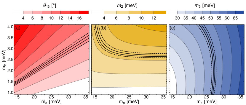
In the $n=3$ case of LSA with $\eta=\frac{2\pi}{3}$ (or LSB with $\eta=-\frac{2\pi}{3}$), all neutrino masses, mixing angles and phases are fully determined from the two remaining parameters $m_{a}$ and $m_{b}$ and the three most precisely measured of these parameters, $\theta_{13}$, $\Delta m^{2}_{31}$ and $\Delta m^{2}_{21}$, currently provide the strongest test of the LS model. Figure 1 shows how these parameters vary in the $m_{a}-m_{b}$ plane, along with the regions corresponding to the $1\sigma$ and $3\sigma$ ranges for these parameters from the NuFit 3.0 (2016) global fit Esteban:2016qun , assuming normal mass ordering and a lightest neutrino mass of $m_{1}=0$. The SD proposal requires $m_{a}$ to be significantly larger than $m_{b}$ and for this portion of the parameter space the approximate proportionality relations of $m_{2}\sim m_{b}$ and $m_{3}\sim m_{a}$ can be seen, verifying the approximations previously derived in King:2015dvf .

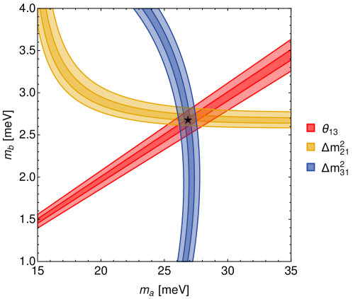
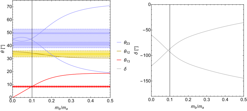
Even at $1\sigma$ the three allowed regions coincide at a single point, as can be seen in Fig. 2, and so this benchmark point can be used to make predictions of the remaining angles $\theta_{12}$ and $\theta_{23}$ and the Dirac phase $\delta$. As described in Section 2 these parameters, along with $\theta_{13}$, depend only on the ratio $r=m_{b}/m_{a}$; this dependence, given by the relations in Eq. 18, is shown in Fig. 3, with the $1\sigma$ and $3\sigma$ NuFIT 3.0 ranges and reference point at $m_{b}/m_{a}=0.1$. For $\theta_{23}$ and $\delta$, the predictions of both LSA and LSB are shown. At this point it can be seen that while both $\theta_{13}$ and $\theta_{12}$ lie within their $1\sigma$ ranges, $\theta_{23}$ lies just outside its $1\sigma$ range, and a prediction on the value of the Dirac phase is made of $\delta\simeq-90^{\circ}$.

Figure 1: Predicted values from LSA with $\eta=\frac{2\pi}{3}$ (or LSB with $\eta=-\frac{2\pi}{3}$) of oscillation parameters depending on the input parameters $m_{a}$ and $m_{b}$. Regions corresponding to the experimentally determined $1\sigma$ (solid lines) and $3\sigma$ (dashed lines) ranges for each parameter are also shown.

Figure 2: Regions in the $m_{a}$-$m_{b}$ plane with fixed $\eta=2\pi/3$ ($\eta=-2\pi/3$) for LSA (LSB) corresponding to the experimentally determined $1\sigma$ and $3\sigma$ ranges for $\theta_{13}$, $\Delta m^{2}_{21}$ and $\Delta m^{2}_{31}$.

Figure 3: Predicted values from LS with fixed $\eta=2\pi/3$ ($\eta=-2\pi/3$) for LSA (LSB) of the mixing angles and delta as a function of the ratio $m_{b}/m_{a}$. Horizontal bands show the experimentally determined $1\sigma$ and $3\sigma$ ranges for each parameter. A reference point giving a good prediction for all parameters is shown at $r=m_{b}/m_{a}=0.1$.

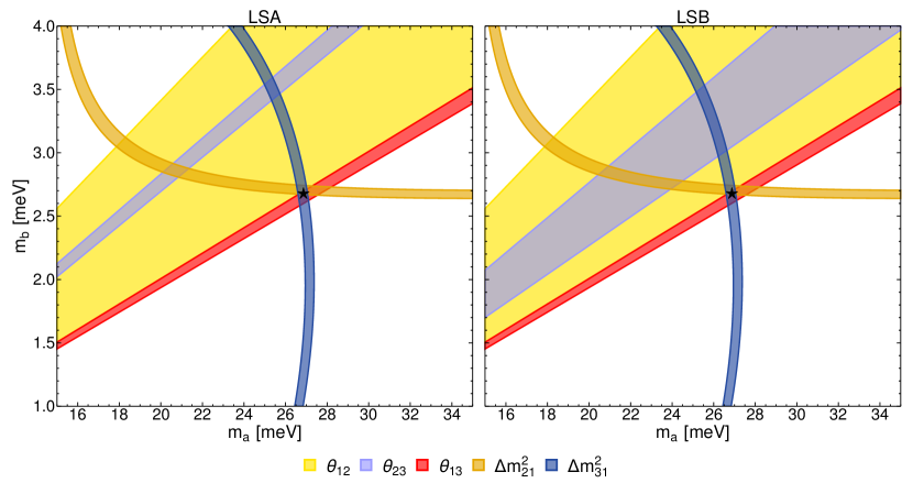
Combining these results for all parameters which have been experimentally measured, displayed together in Fig. 4, it is seen that the prediction for $\theta_{12}$ lies just within current bounds. However, there is tension at the $1\sigma$ level for $\theta_{23}$, due to the allowed regions of LS parameter space requiring values close to maximal, while current data points towards larger deviations from the maximal value. The experimental measurements of $\theta_{23}$ do not yet give consistent indications of its value; while the latest results from NO$\nu$A disfavour maximal mixing at $2.5\sigma$ nova:nu2016 , results from T2K remain fully compatible with maximal $\theta_{23}$ t2k:ichep2016 . As a result, while the combined fit for $\theta_{23}$ is in tension with the LS models at $1\sigma$, the allowed range at $2\sigma$ is far wider, crossing both octants and the maximal value of $45^{\circ}$, including the values preferred by the LS model.

Figure 4: Regions in the $m_{a}$-$m_{b}$ plane with fixed $\eta=2\pi/3$ ($\eta=-2\pi/3$) for LSA (LSB) corresponding to the experimentally determined $1\sigma$ ranges for solar and reactor mixing angles and mass-squared differences. The $\theta_{23}$ regions shown are in tension with other measurements, however, extending to $2\sigma$ these regions become far larger, covering the entire parameter space shown in these plots.

3.2 Predictions of oscillation parameters with $\eta$ as a free parameter

In the versions of the LS models with $\eta$ as an additional free parameter, the mixing angles and phases now depend on both the ratio $r=m_{b}/m_{a}$ and $\eta$. The masses $m_{3}$ and $m_{2}$ depend on all three input parameters; however, their ratio $m_{2}/m_{3}$ (and therefore the ratio $\Delta m^{2}_{21}/\Delta m^{2}_{31}$) will depend only on $r$ and $\eta$. As previously, the strongest contraints come from the very precise measurements of $\theta_{13}$ and the mass-squared differences $\Delta m^{2}_{21}$ and $\Delta m^{2}_{31}$. Figure 5 shows the regions corresponding to the $1\sigma$ ranges for all the mixing angles, $\delta$ and $m_{2}/m_{3}$, where we see that all the five regions come close to overlapping around $\eta=\pm 2\pi/3$ for LSA and LSB, respectively. That two input parameters should give a good description of five observables, within their one sigma errors, is ostensibly a remarkable achievement, indeed perhaps better than might be expected on statistical grounds. However, due to the very tight constraints on $\eta$ from $\theta_{13}$ and $m_{2}/m_{3}$, we still find some tension with the value of $\theta_{23}$ even when allowing $\eta$ to vary. As with the case with $\eta$ fixed, this tension exists only at the $1\sigma$ level, where close to maximal $\theta_{23}$ is excluded.

Figure 5: Regions in the $m_{b}/m_{a}$-$\eta$ plane corresponding to the experimentally determined $1\sigma$ ranges for all mixing angles, $\delta$ and the ratio of neutrino masses $m_{2}/m_{3}$ for LSA (left panel) and LSB (right panel).

3.3 Fitting LS models to global fit data

In order to provide a more concrete measure of the agreement between the predictions of the model and existing data, as well as to make further predictions of the less well measured parameters, we have performed a $\chi^{2}$ fit to the four cases discussed above: LSA and LSB with $\eta$ fixed and free. As a proxy for the full data sets of previous experiments, our fits use the results of the NuFIT 3.0 global analysis Esteban:2016qun . This analysis combines the latest results (as of fall 2016) of solar, atmospheric, long baseline accelerator, and long, medium and short baseline reactor neutrino experiments, to obtain a combined fit to the six standard neutrino oscillation parameters. We use the $\chi^{2}$ data provided by NuFIT, for the case where normal mass ordering is assumed, combining both the 1D $\chi^{2}$ data for each mixing parameter with the 2D $\chi^{2}$ data to include correlations between parameter measurements

$$\chi^{2}_{\text{Fit}}(\Theta)=\sum_{\theta_{i}\in\Theta}\chi^{2}_{\text{1D}}(\theta_{i})+\sum_{\theta_{i}\neq\theta_{j}\in\Theta}\left(\chi^{2}_{\text{2D}}(\theta_{i},\theta_{j})-\chi^{2}_{\text{1D}}(\theta_{i})-\chi^{2}_{\text{1D}}(\theta_{j})\right),$$ (12)

where the first sum in this expression combines each of the 1D $\chi^{2}$ data into a first approximation of the full 6D $\chi^{2}$ while the second sum provides corrections to this coming from the 2D correlations between each pair of parameters.

We then apply this result first to the standard mixing case, then to the LS model case as follows:

• For the case of standard mixing $\Theta=\Theta_{\text{PMNS}}\equiv\left\{\theta_{12},\theta_{13},\theta_{23},\Delta m^{2}_{21},\Delta m^{2}_{31},\delta\right\}$ and we simply combine the NuFIT 3.0 results as shown above, in order to include correlations, and use it to calculate $\chi^{2}\left(\Theta_{\text{PMNS}}\right)\equiv\chi^{2}_{\text{Fit}}(\Theta)$ for this case.

• For the LS model we use instead $\Theta=\Theta_{LS}\equiv\left\{m_{a},m_{b},\eta\right\}$ (or $\Theta_{\text{LS}}=\left\{m_{a},m_{b}\right\}$ when fitting with $\eta$ fixed), which is then minimised over the LS parameter space using the analytic relations to calculate standard mixing parameters from LS parameters, and hence calculate $\chi^{2}\left(\Theta_{\text{LS}}\right)\equiv\chi^{2}_{\text{Fit}}(\Theta)$ for this case.

Our test statistic for a particular LS model is then given by:

$$\sqrt{\Delta\chi^{2}}=\sqrt{\min_{\Theta_{\text{LS}}}\left[\chi^{2}\left(\Theta_{\text{LS}}\right)\right]-\min_{\Theta_{\text{PMNS}}}\left[\chi^{2}\left(\Theta_{\text{PMNS}}\right)\right]}.$$ (13)

We have verified through Monte-Carlo calculations that Wilk’s theorem holds for this statistic, i.e. it is approximately distributed according to a chi-squared distribution.

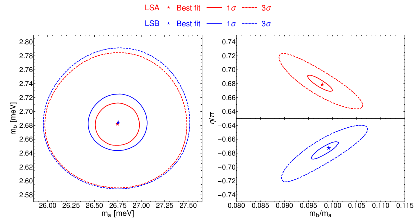
The best fit LSA and LSB points for fits with $\eta$ left free or with $\eta$ fixed at $\frac{2\pi}{3}$ are given in Table 1. The number of degrees of freedom (d.o.f.) is either 3 or 4, which is just the difference between the number of observables (which we take to be the parameters in $\Theta_{\text{PMNS}}$) and the number of LS parameters (namely the parameters in $\Theta_{\text{LS}}$, which is either 3 or 2, depending on whether $\eta$ is free or fixed). For LSA we find a best fit with $\Delta\chi^{2}=4.1$ (3 degrees of freedom) with $\eta$ free and $\Delta\chi^{2}=5.6$ (4 degrees of freedom) fixing $\eta=\frac{2\pi}{3}$, while for LSB we find better fits, with $\Delta\chi^{2}=3.9$ (3 degrees of freedom) and $\Delta\chi^{2}=4.5$ (4 degrees of freedom) for $\eta$ free and $\eta=-\frac{2\pi}{3}$ respectively.

Figure 6 shows the best fit points with $1\sigma$ and $3\sigma$ contours of the fits in the $m_{a}-m_{b}$ plane for fixed $\eta$ and in the $r-\eta$ plane for free $\eta$. The significance at which a LS model is allowed is determined from the distribution of the $\Delta\chi^{2}$ test statistic, where $N\sigma$ has been calculated assuming the that Wilks’ theorem applies. Note that despite LSA predicting values of $\theta_{23}$ which lie outside its individual $1\sigma$ range reported by NuFIT 3.0, there are still regions not excluded at $1\sigma$. This is due to the high predictivity of the model; by predicting many parameters from few input parameters there is a greater chance that one of these may lie outside its experimentally determined range. Statistically, this comes from the increased number of degrees of freedom of the $\chi^{2}$-distribution which approximates our test statistic $\Delta\chi^{2}$.

	LSA		LSB		NuFIT 3.0
	$\eta$ free	$\eta$ fixed	$\eta$ free	$\eta$ fixed	global fit
$m_{a}$ [meV]	27.19	26.74	26.95	26.75
$m_{b}$ [meV]	2.654	2.682	2.668	2.684	—
$\eta$ [rad]	$0.680\pi$	$2\pi/3$	$-0.673\pi$	$-2\pi/3$
$\theta_{12}$ [∘]	34.36	34.33	34.35	34.33	$33.72^{+0.79\phantom{0}}_{-0.76}$
$\theta_{13}$ [∘]	8.46	8.60	8.54	8.60	$8.46^{+0.14\phantom{0}}_{-0.15}$
$\theta_{23}$ [∘]	45.03	45.71	44.64	44.28	$41.5^{+1.3\phantom{00}}_{-1.1}$
$\delta$ [∘]	-89.9	-86.9	-91.6	-93.1	$-71^{+38\phantom{.00}}_{-51}$
$\Delta m^{2}_{21}$ [$10^{-5}\text{eV}^{2}$]	7.499	7.379	7.447	7.390	$7.49^{+0.19\phantom{0}}_{-0.17}$
$\Delta m^{2}_{31}$ [$10^{-3}\text{eV}^{2}$]	2.500	2.510	2.500	2.512	$2.526^{+0.039}_{-0.037}$
$\Delta\chi^{2}$ / d.o.f	4.1 / 3	5.6 / 4	3.9 / 3	4.5 / 4	—

Table 1: Results of our fit of existing data to LSA and LSB with $\eta$ left free and for $\eta=\frac{2\pi}{3}$ for LSA and $\eta=-\frac{2\pi}{3}$ for LSB. The results of the NuFIT 3.0 (2016) global fit to standard neutrino mixing are shown for the normal ordering case for comparison.

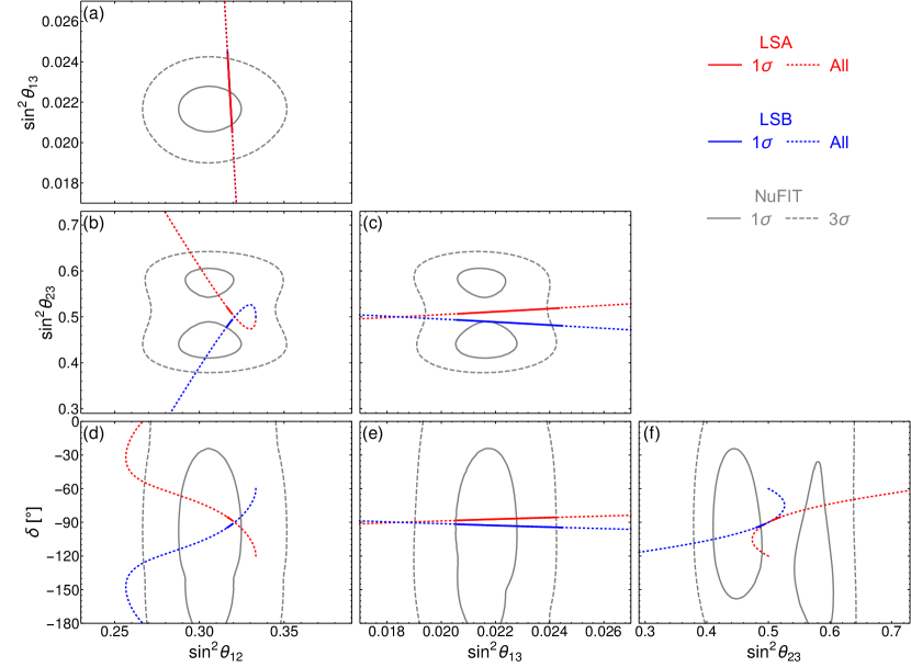
Our fit can also be used to identify the regions of standard neutrino mixing parameter space predicted by LS, once existing data has been taken into account. This corresponds to mapping the regions of LS input parameter space allowed by our fit onto the standard mixing parameter space. Figure 7 shows the predictions of LS (for the fixed $\eta$ case) in the planes made from each pair of mixing angles and $\delta$. Since these values all depend only on the single parameter $r$, the predictions of LS form lines of allowed solutions in each plane, corresponding to sum-rules between the oscillation parameters. For example, Fig. 7a corresponds to the TM1 sum rule in Eq. 6, while Figs. 7b, 7c, 7d, 7e and 7f correspond to those in Eq. 23 or to combinations of these sum rules. It can be seen that very strong restrictions are placed on the allowed values of the less well measured parameters, $\theta_{12}$, $\theta_{23}$ and $\delta$. For the remaining angle, $\theta_{13}$, around two thirds of the NuFIT 3.0 range remains viable in LS.

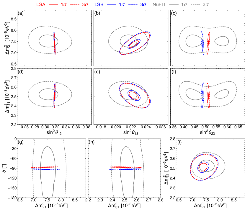
Figure 8 shows the allowed regions of parameter space for pairs of variables including the mass-squared differences. In these plots, as the mass-squared differences can depend on both $m_{a}$ and $m_{b}$ independently, we see regions of allowed values instead of lines. For each of these planes, any point will fully determine both input parameters $m_{a}$ and $m_{b}$, and so these contours correspond exactly to the equivalent regions shown in Fig. 6. In addition to the tight constraints on $\theta_{12}$, $\theta_{23}$ and $\delta$ already mentioned, in Figs. 8b and 8e it can be seen that the allowed range of $\theta_{13}$ is correlated with that of both $\Delta m^{2}_{21}$ and $\Delta m^{2}_{31}$, suggesting that combining future measurements of these parameters could provide a better probe of LS than the individual parameter measurements alone. The ability of future experiment to exclude the model then depends on both the predictions of the model seen here, combined with the sensitivity of experiments to measurements of the parameters in the region of interest predicted by LS, which is the focus of the next section.

Figure 6: Results of the fits to LS of the NuFIT 3.0 (2016) global neutrino oscillation data. Left: LS fit with fixed $\eta=2\pi/3$ ($\eta=-2\pi/3$) for LSA (LSB). Right: LS fit with $\eta$ as a free parameter.

(a)

(b)

(c)

(d)

(e)

(f)

Figure 7: Allowed values for LSA (red) and LSB (blue) with $\eta=2\pi/3$ and $\eta=-2\pi/3$ respectively, showing all possible values (dotted) and the $1\sigma$ range (solid). These lines of allowed solutions correspond to the sum rules in Eqs. 6 and 23, or combinations thereof. Also shown are the $1\sigma$ (solid) and $3\sigma$ (dashed) regions from the NuFIT 3.0 2016 global fit (grey).

(a)

(b)

(c)

(d)

(e)

(f)

(g)

(h)

(i)

Figure 8: Allowed $1\sigma$ (solid) and $3\sigma$ (dashed) regions for LSA (red) and LSB (blue) with $\eta=2\pi/3$ and $\eta=-2\pi/3$ respectively. Also shown are the current allowed regions from the NuFIT 3.0 2016 global fit (grey).

4 Sensitivity of future experiments

In order to understand the potential for future experiments to exclude the LS models, we have performed simulations of a combination of accelerator and reactor experiments, modelling the experimental data expected over the next two decades. We have used the General Long Baseline Experiment Simulator (GLoBES) libraries Huber:2004ka ; Huber:2007ji to simulate future experiments and to fit the simulated data to both standard mixing and the LS models. In all our simulations we assume that the mass ordering is known to be normal ordering, as this is a requirement of the LS models; a measurement of inverted ordering would immediately exclude the models.

4.1 Future neutrino oscillation experiments

Our combination of experiments include detailed simulations of the T2HK and DUNE long-baseline accelerator experiments, which aim to provide precision measurements of $\Delta m^{2}_{31}$, $\theta_{23}$ and $\delta$, together with basic constraints on $\theta_{13}$ from the Daya Bay short baseline reactor experiment and on $\theta_{12}$ and $\Delta m^{2}_{21}$ from the JUNO and RENO-50 medium baseline reactor experiments. We will now briefly recap the salient features of these experiments and our treatment of them.

T2HK

The Tokai to Hyper-Kamiokande (T2HK) experiment is a proposed long-baseline accelerator neutrino experiment using the Hyper-Kamiokande detector, a megatonne scale water Cherenkov detector to be constructed near to the Super-Kamiokande detector in Kamioka, Japan HKDR . The standard design is for two tanks to be built, each with 258 kt (187 kt) of total (fiducial) volume. The tanks are to be built in a staged process with the second tank constructed and commissioned after the first, such that the second begins to take data six years after the first. The water Cherenkov technique is capable of detecting the (anti-)muons and electrons (positrons) produced in (anti-)neutrino interactions, with the ability to distinguish the charged leptons’ flavours but not their charge. The detector would be used to observe neutrinos from (amongst other sources) an upgraded version of the T2K neutrino beam produced at J-PARC in Tokai, $L=295$ km from the detector. The 1.3 MW beam, produced from a 30 GeV protons, is directed 2.5^∘ away from the detector in order to provide a narrow energy spectrum at the far detector peaked around the first atmospheric neutrino oscillation maximum for $\Delta m^{2}_{31}\sim 2.5\times 10^{-3}$ eV² and $E=0.6$ GeV. Either $\nu_{\mu}$ or $\bar{\nu}_{\mu}$ can be produced as the principle component of the beam, such that the oscillation probabilities $P(\nu_{\mu}\to\nu_{e})$, $P(\bar{\nu}_{\mu}\to\bar{\nu}_{e})$, $P(\nu_{\mu}\to\nu_{\mu})$ and $P(\bar{\nu}_{\mu}\to\bar{\nu}_{\mu})$ can all be measured. While the main goal of T2HK is to search for CP symmetry violation by observing a non-CP conserving value of $\delta$, precision measurements of $\theta_{23}$ and the magnitude of $\Delta m^{2}_{31}$ will also be made Abe:2015zbg .

DUNE

The Deep Underground Neutrino Experiment Acciarri:2016crz (DUNE) is a proposed long-baseline accelerator experiment, which differs from the T2HK experiment through its longer baseline and higher energy wide-band beam. The experiment will use a new neutrino beam sourced at Fermilab, directed towards a large liquid argon detector in Sanford, $L=$1300 km from the beam source. The 40 kt LArTPC detector is able to detect both the charged leptons and the hadrons produced from muon and electron (anti-)neutrino interactions, with strong particle identification and energy reconstruction capabilities. The standard design is for a 1.07 MW $\nu_{\mu}$ or $\bar{\nu}_{\mu}$ beam produced from 80 GeV protons, with an on-axis design to produce a wide energy spectrum spanning $E=$0.5 to 5 GeV, allowing observations of the $\nu_{e}$ appearance spectrum around the first atmospheric neutrino oscillation maximum for $\Delta m^{2}_{31}\sim 2.5\times 10^{-3}$ eV². While measuring the same oscillation channels as T2HK, the wider band beam with longer baseline provides complementary information on the value of $\delta$ as well as measurements of $\theta_{23}$ and, due to the matter effects from the longer baseline, both the sign and the magnitude of $\Delta m^{2}_{31}$ Acciarri:2015uup .

Short baseline reactor experiments

By observing the oscillations of the $\bar{\nu}_{e}$ produced in nuclear reactors, short baseline reactor neutrino experiments are able to measure the mixing angle $\theta_{13}$ with particularly high accuracy. The Daya Bay experiment Guo:2007ug currently has the most precise measurement of this parameter with the aim to achieve a precision on $\sin^{2}\theta_{13}$ of better than 3% Cao:2016vwh . The experiment measures anti-neutrinos produced in six nuclear reactors in south China. A total of eight 20 t liquid scintillator detectors are used; two are located at each of two near detector sites and four at a far detector site $L=$1.5 to 1.9 km from the reactors near the first atmospheric neutrino oscillation maximum for $\Delta m^{2}_{31}\sim 2.5\times 10^{-3}$ eV², given the low nuclear energy of the neutrino beam $E\sim$ few MeV. Results of the Double Chooz Ardellier:2004ui and RENO Ahn:2010vy ; Kim:2014rfa short baseline reactor experiments also contribute to the precision obtained on $\theta_{13}$ combined with the Daya Bay result. Although DUNE and T2HK will also measure this parameter with high precision, the measurement of the short baseline reactor programme by that time is expected to be at least as precise, and will provide a measurement independent of the other parameters which influence the appearance channel at long-baseline accelerator experiments.

Medium baseline reactor experiments

The Jiangmen Underground Neutrino Observatory Djurcic:2015vqa (JUNO) and the future plans of the Reactor Experiment for Neutrino Oscillation (RENO-50) Kim:2014rfa are medium baseline reactor neutrino experiments which, like the Daya Bay experiment, will observe the oscillations of electron anti-neutrinos produced in nuclear reactors. The JUNO experiment will use a 20 kt liquid scintillator detector approximately $L=$53 km from two planned nuclear reactors in southern China, while RENO-50 will use an 18 kt liquid scintillator detector approximately $L=$50 km from a nuclear reactor in South Korea. Given the low nuclear energy of the neutrino beam $E\sim$ few MeV, these longer baselines correspond to the first solar neutrino oscillation maximum for $\Delta m^{2}_{21}\sim 7.5\times 10^{-5}$ eV², where the higher frequency atmospheric oscillations appear as wiggles. Thus the longer baseline than at Daya Bay gives greatest sensitivity to a different set of oscillation parameters, in particular $\theta_{12}$ and $\Delta m^{2}_{21}$. The precision on the measurements of both $\sin^{2}\theta_{12}$ and $\Delta m^{2}_{21}$ is expected to reach 0.5% Djurcic:2015vqa ; Kim:2014rfa .

Details of experimental simulation

Experiment	Parameter	Precision
Short baseline reactor	$\sin^{2}\theta_{13}$	3%
Medium baseline reactor	$\sin^{2}\theta_{12}$	0.5%
Medium baseline reactor	$\Delta m^{2}_{21}$	0.5%

Table 2: Precision of oscillation parameter measurements made by reactor experiments which we have used as constraints in our simulations.

We have used complete simulations of the latest designs for both DUNE and T2HK where we have assumed both experiments run for 10 years. Full details of the GLoBES implementations we have used can be found in synergy . For the short and medium baseline reactor experiments, we have included basic constraints on the values of $\sin^{2}\theta_{13}$, $\sin^{2}\theta_{12}$ and $\Delta m^{2}_{21}$. Since these measurements are expected to be approximately independent of other parameters we have implemented these constraints as simple Gaussian measurements with a mean of the true simulated value and error as given in Table 2.

4.2 Statistical method

To determine the statistical significance with which the LS model could be excluded based on simulated data, we perform a minimum-$\chi^{2}$ fit to both standard three neutrino mixing and to the LS model. As in section 3.3, for the case of standard mixing we use $\Theta=\Theta_{\text{PMNS}}\equiv\left\{\theta_{12},\theta_{13},\theta_{23},\Delta m^{2}_{21},\Delta m^{2}_{31},\delta\right\}$, while for LS we use $\Theta=\Theta_{LS}\equiv\left\{m_{a},m_{b},\eta\right\}$ (or $\Theta_{\text{LS}}=\left\{m_{a},m_{b}\right\}$ when fitting with $\eta$ fixed). Our test statistic for the significance to exclude the LS model is then given by

$$\sqrt{\Delta\chi^{2}}=\sqrt{\min_{\Theta_{\text{LS}}}\left[\chi^{2}\left(\Theta_{\text{LS}}\right)\right]-\min_{\Theta_{\text{PMNS}}}\left[\chi^{2}\left(\Theta_{\text{PMNS}}\right)\right]}.$$ (14)

The significance at which LS is excluded is then determined from the distribution of the $\Delta\chi^{2}$ test statistic; where we give sensitivities in terms of $N\sigma$, this quantity has been calculated assuming the that Wilks’ theorem applies. Wilks’ theorem states that when comparing nested models, the $\Delta\chi^{2}$ test statistic is a random variable asymptotically distributed according to the $\chi^{2}$-distribution with the number of degrees of freedom equal to the difference in number of free parameters in the models. In this case we treat the LS models, with two or three free parameters, as sub-models of standard neutrino mixing with six free parameters, leading to a $\chi^{2}$-distribution with 4 degrees of freedom when $\eta$ is kept fixed or 3 degrees of freedom when $\eta$ is left as a free parameter. We have verified via Monte-Carlo simulations that the distribution of our $\Delta\chi^{2}$ test statistic is well approximated by these distributions.

In applying the above formula, the $\chi^{2}(\Theta)$ is minimised over the parameters $\Theta$ in our fits and is built from three parts;

$$\chi^{2}(\Theta)=\chi^{2}_{\text{LB}}(\Theta)+\chi^{2}_{\text{R}}(\Theta)+P(\Theta),$$ (15)

with $\chi^{2}_{\text{LB}}(\Theta)$ for the full simulations of the long-baseline experiments DUNE and T2HK, $\chi^{2}_{\text{R}}(\Theta)$ for the constraints from reactor experiments Daya Bay and JUNO, and $P(\Theta)$ for a prior intended to include information from the results of existing experimental measurements.

For the long-baseline experiments we use the statistical model of the GLoBES library Huber:2004ka ; Huber:2007ji , where the $\chi^{2}_{LB}(\Theta)$ is a sum of contributions from each of the experiments’ channels. The individual contributions are constructed as

$$\chi^{2}_{c}(\Theta)=\min_{\xi=\{\xi_{s},\xi_{b}\}}\left[2\sum_{i}\left(\eta_{i}(\Theta,\xi)-n_{i}+n_{i}\ln\frac{n_{i}}{\eta_{i}(\Theta,\xi)}\right)+p(\xi,\sigma)\right],$$ (16)

where $\chi^{2}_{c}$ denotes the contribution from a given channel of a given experiment. The sum in this expression is over the $i$ energy bins of the experimental configuration, with simulated true event rates of $n_{i}$ and simulated event rates $\eta_{i}(\Theta,\xi)$ for the hypothesis parameters $\Theta$ and systematic error parameters $\xi$. The systematic errors of the experiments are treated using the method of pulls, parameterized as $\xi_{s}$ for the signal error and $\xi_{b}$ for the background error. These parameters are given Gaussian priors which form the term $p(\xi,\sigma)=\xi_{s}^{2}/\sigma_{s}^{2}+\xi_{b}^{2}/\sigma_{b}^{2}$, where $\sigma=\{\sigma_{s},\sigma_{b}\}$ are the sizes of the systematic errors given by the experiment.

For the reactor experiments we simply assume independent Gaussian measurements such that

$$\chi^{2}_{\text{R}}=\frac{\left(\sin^{2}{\theta_{13}}-\sin^{2}\overline{\theta_{13}}\right)^{2}}{\sigma_{\theta_{13}}^{2}}+\frac{\left(\sin^{2}{\theta_{12}}-\sin^{2}\overline{\theta_{12}}\right)^{2}}{\sigma_{\theta_{12}}^{2}}+\frac{\left(\Delta m^{2}_{21}-\overline{\Delta m^{2}_{21}}\right)^{2}}{\sigma_{\Delta m^{2}_{21}}^{2}},$$ (17)

where $\overline{\theta_{13}}$, $\overline{\theta_{12}}$ and $\overline{\Delta m^{2}_{21}}$ are the true parameter values and $\sigma_{\theta_{13}}$, $\sigma_{\theta_{12}}$ and $\sigma_{\Delta m^{2}_{21}}$ the corresponding experimental measurement uncertainties.

The prior $P(\Theta)$ provides information from existing experimental measurements and is calculated using the results of the NuFIT 3.0 global fit in the same way as our fit in Section 3.3, so that $P(\Theta)=\chi^{2}_{\text{Fit}}(\Theta)$ as defined in Eq. 12.

In all our simulations, the true parameters are taken to be the best-fit values from the appropriate LS fit results given in Table 1, except where stated otherwise.

4.3 Results

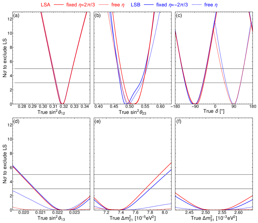
The sensitivity to exclude either version of the LS model is shown as a function of the true value of each parameter in Fig. 9, for true values, with the range selected along the horizontal axes to be that given by the currently allowed at $3\sigma$ by the latest NuFIT 3.0 global fit. In each case, the parameters not shown are assumed to take their best-fit values from the fit to LS described in Section 3.3.

From the upper panels in Fig. 9, we see that $\theta_{12}$, $\theta_{23}$ and $\delta$ provide the strongest tests of the model, with there only being a relatively small portion of the presently allowed true parameter space where the model would not be excluded. This is due to the strong predictions of these parameters by the LS models, as discussed in Section 3.1. Note that these parameters are those that will be measured most precisely by the three next-generation experiments used in our simulations, JUNO, DUNE and T2HK. For these three parameters, the effect of allowing $\eta$ to vary does not much change the sensitivity, other than the additional solution (currently disfavoured by experiment) with $\delta=+90^{\circ}$ which occurs when changing the sign of $\eta$. For $\theta_{12}$ in particular there is no effect of allowing $\eta$ to vary. This is due to the sum rule in Eq. 6 which relates $\theta_{12}$ with $\theta_{13}$ independently from the value of $\eta$; the precise measurement of $\theta_{13}$ then fixes the value of $\theta_{12}$ to a narrow range such that a measurement of $\theta_{12}$ outside of this would exclude the LS model regardless of the LS parameter values. Similarly the precise measurements of $\theta_{13}$, $\Delta m^{2}_{21}$ and $\Delta m^{2}_{31}$ strongly constrain the magnitude (but not sign) of $\eta$, so that the LS allowed regions of the other variables are not significantly changed when $\eta$ is allowed to vary, with the noted exception that changing the sign of $\eta$ allows the sign of $\delta$ to also change.

From the lower panels in Fig. 9, we see that the sensitivity to exclude LS from measurements of $\theta_{13}$, $\Delta m^{2}_{21}$ or $\Delta m^{2}_{31}$ is much less than for the other three parameters and the sensitivity is also significantly reduced when allowing $\eta$ to vary. By the converse argument to that used above, this is due to these three parameter measurements driving the fit to $m_{a}$ and $m_{b}$ (and $\eta$), and so a measurement of these parameters will tend to move the fitted LS parameter values rather than exclude the model, particularly when fitting the extra free parameter $\eta$. However, a particularly small measurement of $\theta_{13}$ or particularly large measurement of $\Delta m^{2}_{21}$, relative to their current allowed range of values, may still exclude the fixed $\eta$ version of the models.

(a)

(b)

(c)

(d)

(e)

(f)

Figure 9: The predicted sensitivity of future experiments to excluding LSA (red) and LSB (blue), shown as a function of the true value of each parameter. Solid curves correspond to the case with $\eta$ fixed at $\eta=\frac{2\pi}{3}$ for LSA or $\eta=-\frac{2\pi}{3}$ for LSB, while dashed curves correspond to the case with $\eta$ left free. The ranges of true parameters shown in the plots corresponds to the current three sigma allowed NuFIT 3.0 regions.

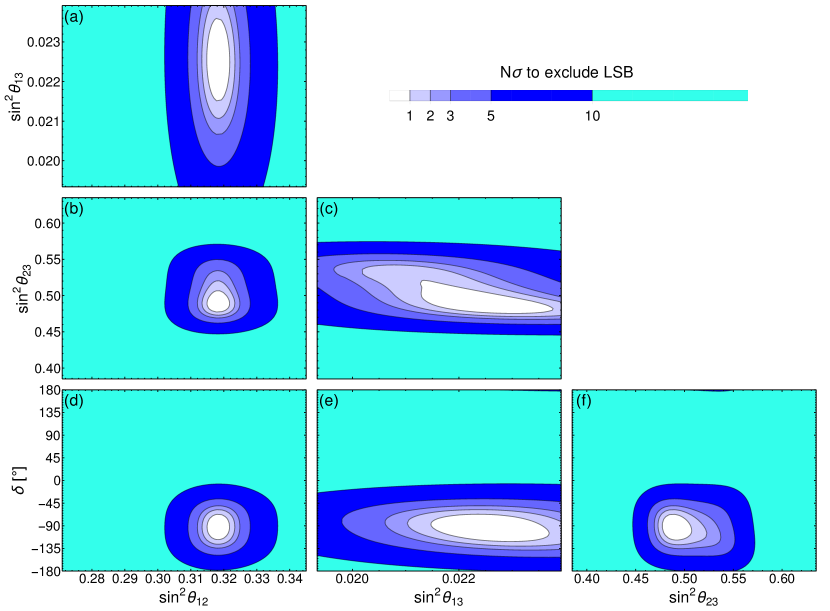
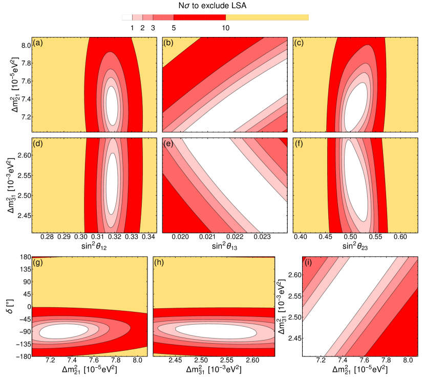
The results shown in Fig. 9 show only the dependence of the significance to exclude LS on the true value of each variable individually. However, the sensitivity will generally have a strong dependence on the true values of the other parameters. The significance to exclude the LS models depending on the true values of each pair of variables, for the cases where $\eta$ is kept fixed, is shown in Figures 10 and 12 for LSA and in Figs. 11 and 13 for LSB.

Each panel of Figs. 10 and 11 includes two dimensionless variables (i.e. angle or phase) which both depend only on the ratio of LS input parameters $r=m_{b}/m_{a}$, and so, in a LS model, a measurement of any one of these parameters corresponds to a measurement of $r=m_{b}/m_{a}$ (see Fig. 3). Combining two of these parameter measurement therefore give two measurements of $r=m_{b}/m_{a}$, with any conflict between them providing strong evidence to exclude the model. For this reason the significance to exclude the models is close to being simply the combined significance from individual measurements implied by Fig. 9.

By contrast, each panel of Figures 12 and 13 shows the results for the pairs of variables including at least one dimensionful mass-squared difference. Here we can see in Figs. 12b, 12e and 12i for LSA, and in Figs. 13b, 13e and 13i for LSB, there is a strong correlation between the measurements of $\theta_{13}$, $\Delta m^{2}_{21}$ and $\Delta m^{2}_{31}$. This shows clearly that, although individual measurements of these parameters cannot exclude a LS model (since the parameters of the LS model could be adjusted to accommodate any of them individually) a combined measurement of two of them could serve to exclude the model. This is the reason for presenting these combined sensitivity plots. Of the three parameters for which such combined measurements provide the strongest test of the model, each pair includes measurements from different experiments, with $\theta_{13}$ coming mainly from the short-baseline reactor measurement such as Daya Bay, $\Delta m^{2}_{21}$ from the medium-baseline reactor measurement such as JUNO, and $\Delta m^{2}_{31}$ from the long-baseline accelerator measurement such as DUNE and T2HK. This demonstrates a strong synergy between all these experiments in attempts to exclude the LS models.

(a)

(b)

(c)

(d)

(e)

(f)

Figure 10: The predicted sensitivity of future experiments to excluding LSA, with $\eta$ fixed at $\eta=\frac{2\pi}{3}$, shown as a function of each pair of true parameters. The ranges of true parameters shown in the plots corresponds to the current three sigma allowed NuFIT 3.0 regions.

(a)

(b)

(c)

(d)

(e)

(f)

Figure 11: The predicted sensitivity of future experiments to excluding LSB, with $\eta$ fixed at $\eta=-\frac{2\pi}{3}$, shown as a function of each pair of true parameters. The ranges of true parameters shown in the plots corresponds to the current three sigma allowed NuFIT 3.0 regions.

(a)

(b)

(c)

(d)

(e)

(f)

(g)

(h)

(i)

Figure 12: The predicted sensitivity of future experiments to excluding LSA, with $\eta$ fixed at $\eta=\frac{2\pi}{3}$, shown as a function of each pair of true parameters. The ranges of true parameters shown in the plots corresponds to the current three sigma allowed NuFIT 3.0 regions.

(a)

(b)

(c)

(d)

(e)

(f)

(g)

(h)

(i)

Figure 13: The predicted sensitivity of future experiments to excluding LSB, with $\eta$ fixed at $\eta=-\frac{2\pi}{3}$, shown as a function of each pair of true parameters. The ranges of true parameters shown in the plots corresponds to the current three sigma allowed NuFIT 3.0 regions.

5 Conclusion

In this paper, we have investigated the ability to probe one of the most predictive viable neutrino mass and mixing models with future neutrino oscillation experiments: the Littlest Seesaw. The LS models work within the framework of the Type I seesaw mechanism, using two right-handed neutrinos to generate the left-handed neutrino masses. Combined with constraints from flavour symmetries, the neutrino mixing angles and phases can be predicted from a small number of parameters; in its most constrained form all neutrino masses, angles, and phases are determined from just two input parameters. In fact, we have shown that while the neutrino masses depend on the two mass parameters independently, the mixing angles and phases depend only on a single dimensionless quantity, the ratio of these two input parameters.

We have studied two versions of this model (LSA and LSB) which use different flavour symmetries to enforce constraints which result in different permutations of the second and third rows and columns of the neutrino mass matrix, leading to different predictions for the octant of $\theta_{23}$. Using the results of a recent global fit of neutrino oscillation experiments, we have found that both versions can well accommodate the parameter values as measured by experiment, with the greatest tension on the value of $\theta_{23}$ at the $1\sigma$ level. The prediction of LS is very close to the maximal mixing value with experimental results from NO$\nu$A suggesting a more non-maximal value, while results from T2K still consistent with a maximal value of $\theta_{23}$. We find that the LSB version, predicting a value of $\theta_{23}$ in the lower octant, to be slightly preferred.

The ability of future experiments to exclude these models then comes from a convolution of the strength of the predictions of the model with the sensitivity of the experiments in measuring those parameters. Through our fit of the models to current global neutrino oscillation data, we have seen that the LS models make strong predictions for the values of $\theta_{12}$, $\theta_{23}$, and $\delta$, the three parameters for which current measurements are weakest. In addition we find that, for certain combinations of the remaining observables, $\theta_{13}$, $\Delta m^{2}_{21}$ and $\Delta m^{2}_{31}$, the LS models predict strong correlations.

With future experiments expected to improve precision on all six parameters measured through oscillations, our simulations have shown that the LS models can be thoroughly tested through future precise individual measurements of $\theta_{12}$, $\theta_{23}$, and $\delta$. This can be readily understood since the free parameters of the LS models are currently most constrained by the precise measurements of $\theta_{13}$, $\Delta m^{2}_{21}$ and $\Delta m^{2}_{31}$, leading to predictions for the currently less well determined parameters $\theta_{12}$, $\theta_{23}$, and $\delta$.

The predictivity of the LS models means that an even higher precision measurement of those parameters which currently drive the fit of the input parameters, namely $\theta_{13}$, $\Delta m^{2}_{21}$ and $\Delta m^{2}_{31}$, could still exclude the LS models when considered in combination with each other. For example, the combination of any two of them could require a region of LS parameter space already excluded by the third.

These above results all highlight the strong complementarity between different classes of oscillation experiment. While the long baseline accelerator experiments DUNE and T2HK are expected to provide the strongest measurements of $\theta_{23}$ and $\delta$ (two of those that can individually test the model’s viability) the third, $\theta_{12}$, will come from medium baseline reactor experiments such as JUNO and RENO-50. The strongest complementarity, however, comes from combining precision measurements of $\Delta m^{2}_{21}$, $\Delta m^{2}_{31}$ and $\theta_{13}$, where any pair of these measurements relies on the results from all the different experiments: long-baseline accelerator experiments for $\Delta m^{2}_{31}$, medium-baseline reactor experiments for $\Delta m^{2}_{21}$, and short-baseline reactor experiments for $\theta_{13}$.

In summary, the work presented in this paper shows that the most straightforward way to exclude the LS model is to provide a better individual determination of the three currently less precisely measured parameters $\theta_{12}$, $\theta_{23}$, and $\delta$, which requires both medium baseline experiments such as JUNO and RENO-50, and long baseline experiments such as DUNE and T2HK, where the synergy between the latter two experiments is thoroughly explored in synergy . In addition, the LS model could be constrained by combined measurements of the three remaining parameters $\Delta m^{2}_{21}$, $\Delta m^{2}_{31}$ and $\theta_{13}$, where an even higher precision of the latter reactor parameter at the short baseline Daya Bay experiment can also play an important role.

We remark that, although the above conclusions have been established for the LSA and LSB models, similar arguments can be expected to apply to any highly predictive flavour models which determine the oscillation parameters from a smaller number of input model parameters. In any such model, the input parameters will tend to be tuned to fit the strong constraints from the most precisely measured parameters, leading to predictions of the other parameters. If the models can accommodate individual measurements in this way, distinguishing between them using those parameters which drive the fit is still possible, if those models are highly constrained, but this requires the parameter measurements to be considered in combination.

In conclusion, the need for future reactor and accelerator experiments to measure individually $\theta_{12}$, $\theta_{23}$ and $\delta$, plus combinations of $\theta_{13}$, $\Delta m^{2}_{21}$ and $\Delta m^{2}_{31}$, may be considered to be general requirements in order to probe predictive flavour symmetry models. Therefore a broad programme of such precision experiments seems to be essential in order to take the next step in understanding neutrino oscillations in the context of the flavour puzzle of the Standard Model.

Appendix

Appendix A Exact expressions for LS sum rules

The angles and Dirac phase can then be written as

$$\sin^{2}\theta_{13}=s(r),\qquad\tan^{2}\theta_{12}=t(r),\qquad\cos 2\theta_{23}=\pm c(r),\qquad\cos\delta=\pm d(r),$$ (18)

with positive signs taken for LSA and negative for LSB and where

$$s(r)= \frac{1}{6}\left(1-\frac{55r^{2}+4(1-4r)}{\sqrt{\left((11r)^{2}+4(1-7r)\right)\left((11r)^{2}+4(1-r)\right)}}\right)$$ (19)

$$t(r)= \frac{1}{4}\left(1+\frac{55r^{2}+4(1-4r)}{\sqrt{\left((11r)^{2}+4(1-7r)\right)\left((11r)^{2}+4(1-r)\right)}}\right)$$ (20)

$$c(r)= \frac{2r(11r-1)\left(55r^{2}-16r+4-5\sqrt{\left((11r)^{2}+4(1-7r)\right)\left((11r)^{2}+4(1-r)\right)}\right)}{\left((11r)^{2}+4(1-7r)\right)\left((11r)^{2}+4(1-r)\right)+4r^{2}\left((11r)^{2}+2(2-11r)\right)}$$ (21)

$$d(r)= -\frac{c(r)(1-5s(r))}{2\sqrt{2s(r)(1-c(r)^{2})(1-3s(r))}}.$$ (22)

Similar expressions for the Majorana phases also possible. Combining these, expressions relating any two of the angles and/or phases can be found. The first such relation, relating $\theta_{13}$ and $\theta_{12}$, is the same as Eq. 6, which is general for all CSD($n$). New exact relations between $\theta_{13}$ and $\theta_{23}$ or $\theta_{12}$ and $\theta_{23}$, as well as the relation between $\delta$ and $\theta_{12}$, true for LSA with $\eta=\frac{2\pi}{3}$ or LSB with $\eta=-\frac{2\pi}{3}$, are found of the form

$$f_{\pm}(\theta_{13},\theta_{23})=0,\qquad g_{\pm}(\theta_{12},\theta_{23})=0,\qquad h_{\pm}(\delta,\theta_{12})=0,$$ (23)

where again the positive (negative) sign is used in the functions valid for LSA (LSB). Exact expressions are given as

$$f_{\pm} (\theta_{13},\theta_{23})=\frac{44s_{13}^{2}\sqrt{1-3s_{13}^{2}}}{4(1-6s_{13}^{2})\mp 3c_{13}^{2}\cos 2\theta_{23}}\pm\frac{c_{13}^{2}\cos 2\theta_{23}}{\sqrt{1-3s_{13}^{2}}}-\sqrt{\frac{8s_{13}^{2}}{3}-\frac{c_{13}^{4}\cos^{2}2\theta_{23}}{3(1-3s_{13}^{2})}},$$ (24)

$$g_{\pm} (\theta_{12},\theta_{23})=\frac{22s_{12}^{2}\sqrt{1-3s_{12}^{2}}}{2(5s_{12}^{2}-1)\mp\cos 2\theta_{23}}\pm\frac{\cos 2\theta_{23}}{\sqrt{1-3s_{12}^{2}}}-\sqrt{4s_{12}^{2}-\frac{\cos^{2}2\theta_{23}}{3(1-3s_{12}^{2})}},$$ (25)

$$h_{\pm} (\delta,\theta_{12})=\frac{5s_{12}^{2}-1}{s_{12}\sqrt{1-3s_{12}^{2}}}\pm\frac{\sqrt{3}\cos\delta}{\sqrt{1-12s_{12}^{2}(1-3s_{12}^{2})\sin^{2}\delta}}+\frac{11\sqrt{1-12s_{12}^{2}(1-3s_{12}^{2})\sin^{2}\delta}}{2(6s_{12}^{2}-1)\sin\delta\mp 2\sqrt{3}\cos\delta}.$$ (26)