Relaxation dynamics of two coherently coupled one-dimensional bosonic gases

Abstract

In this work we consider the non-equilibrium dynamics of two tunnel coupled bosonic gases which are created from the coherent splitting of a one-dimensional gas. The consequences of the tunneling both in the non-stationary regime as well as at large time are investigated and compared with equilibrium results. In particular, within a semiclassical approximation, we compute correlation functions for the relative phase which are experimentally measurable and we observe a transient regime displaying oscillations as a function of the distance. The steady regime is very well approximated by a thermal state with a temperature independent of the tunneling strength.

1 Introduction

Thanks to the great achievements in the field of cold atomic experiments the recent theoretical research interest on the dynamics of closed quantum systems has increased enormously Altman_2105 ; RSLS_2015 ; PSSV2011 . This class of experiments allows one to prepare the system in highly excited states in a controllable manner, also because of the high tunability of the underlying Hamiltonians, to monitor their dynamics in isolation from the coupling to any environment and to probe the system under appropriate time scales BDZ2008 ; langen2014 .

In this context some relevant questions that can be addressed from the theoretical and the experimental point of view are connected with the properties of the relaxation of such excited state, with the approach of a possible steady regime and with the emergence or not of a canonical (or a generalized) thermal state greiner2002 ; KWW2006 ; Gring_Science_2012 ; LEGRSKRMGS2014 ; schreiber2015 .

The understanding of how thermalization occurs in isolated quantum systems have actually been investigated long time ago S1994 and is now subject to a revival of interest. Moreover, the comprehension of the relaxation dynamics of isolated many-body systems is of crucial importance also to have under control the experiments where cold atomic systems are designed to probe equilibrium phases as they inevitably evolve in absence of coupling to a thermal bath which ensures the thermalization of the system.

In this dynamical setting a lot of attention has been devoted to the understanding of the role of integrability and the stationary ensemble that is reached under this constraint VR_2016 ; CEF_2011 ; IDNWBC_2015 ; CK_2012 ; CIC_2012 ; mussardo2013 . In particular, due to the presence of integrals of motion, many theoretical works have pointed out the emergence of many (an extensive number of) temperatures or chemical potentials that ensure the conservation of local quantities. Experimentally the existence of many generalized temperatures (or generically Lagrange multipliers) in a nearly integrable system have been shown in LEGRSKRMGS2014 .

However the macroscopic differences between a generalized or a standard Gibbs ensemble are not always very pronounced and it is important to understand when this happens and if there are constants of motion more constraining than others.

Moreover both from the theoretical and the experimental point of view it is natural to ask about the effect of perturbations on such generalized ensembles and when a genuine thermalization of the system occurs. True thermalization is a time dependent phenomenon which might have very long time scales and preceded by a transient pre-thermal state. In berges2004 prethermalization was presented as the equilibration at short times of some thermodynamic quantities while some other being still out-of-equilibrium, which is succeeded on a much larger time scale by the full equilibration of all observables. A prethermalized state was experimentally observed in Gring_Science_2012 and interpreted as the decoupling of two types of modes in the system. From a renormalization group perspective it is interesting that integrability breaking interactions that at equilibrium might be irrelevant in a non equilibrium unitary dynamics can drive the system to stationary states with different properties than the integrable ones where eventually a single thermodynamic temperature governs the dynamics MG_2011 .

This work is inspired by a set of remarkable experimental and theoretical achievements on the understanding of the relaxation dynamics of quantum many-body systems that have been carried on in a long series of works Gring_Science_2012 ; LEGRSKRMGS2014 ; KISD11 ; SMLK2013 ; LGKRS13 ; LGS_2016 . In these works they considered a one-dimensional gas of bosons which is suddenly split into two one-dimensional gases, sharing almost the same phase profile. In all these works the two gases after the splitting were independent (one controlled way to study the splitting is provided the ladder system FG2015 ). The goal of the present study is to consider the effect of a tunnel coupling term between the two gases after the splitting is performed. We study how this term changes the relaxation of correlation functions that can be directly measured in interference measurements and its consequences on the effective temperature that emerged from the pretehrmalized state in Gring_Science_2012 .

The manuscript is organized as follows: in Section 2 and 3 we present the model and the characterization of the initial state, in section 4 we describe the thermodynamic and dynamic properties of the eigenmodes, in section 5 we discuss the dynamics of the relative phase of the two gases and we compare with the equilibrium values, in section 6 we study two-time quantities and we look at fluctuation-dissipation relations. Finally in section 7 we discuss our results and we conclude.

2 Theoretical setting

The system is prepared as a one-dimensional gas and, at time $t=0$, a barrier is grown in order to create two one-dimensional systems sharing almost the same phase profile KISD11 ; Gring_Science_2012 ; LGKRS13 . We suppose that the barrier is grown instantaneously and kept finite. In Fig. 1 we show a sketch of this situation.

The Hamiltonian of the two systems after the splitting is well described within the Luttinger liquid theory by giamarchi2004 :

$$H=H_{LL}^{1}+H_{LL}^{2}-\,\frac{t_{\perp}}{2\pi}\,\int{\rm d}x\,2\cos(\theta_{2}(x)-\theta_{1}(x))\ .$$ (1)

Here $H_{LL}^{\alpha}$ is the Luttinger liquid Hamiltonian describing the system $\alpha=1,2$:

$$H_{LL}^{\alpha}=\frac{\hbar u}{2}\int{\rm d}x\,\Big{[}\,\frac{\mathcal{K}}{\pi}\,[\nabla\theta_{\alpha}(x)]^{2}\,+\,\frac{\pi}{\mathcal{K}}[n_{\alpha}(x)]^{2}\,\Big{]}\ ,$$ (2)

$u$ is the sound velocity and $\mathcal{K}$ is the Luttinger parameter which encodes the interactions of the system: $\mathcal{K}=1$ corresponds to hard core bosons while $\mathcal{K}=\infty$ to free bosons. The operators $\theta(x)$ and $n(x)$ representing respectively the phase of the bosonic field and the fluctuation of its density are canonically conjugated: $[n(x),\theta(x^{\prime})]=i\delta(x-x^{\prime})$. The cosine term originates from the tunneling operator $\psi_{1}^{{\dagger}}(x)\psi_{2}(x)+{\rm h.c.}=2\,\rho\cos(\theta_{2}(x)-\theta_{1}(x))$, where we used that $\psi_{\alpha}(x)\simeq\sqrt{\rho}\,e^{i\theta_{\alpha}(x)}$ and $\rho$ is the density. Therefore one can set $t_{\perp}=\,\hbar\,J\rho$, where $\hbar J$ is the energy scale defined by the potential barrier.

Figure 1: Schematic figure of the splitting protocol that leads from one single gas to two tunnel-coupled tubes.

The dynamics of this system can be studied by introducing symmetric and antisymmetric variables $\theta_{A/S}=\theta_{1}\mp\theta_{2}$ and $n_{A/S}=(n_{1}\mp n_{2})/2$. Indeed under the assumption that the two systems are identical, symmetric and antisymmetric modes decouple and in terms of those variables one has $H=H_{LL}^{S}+H_{SG}^{A}$ with $H_{SG}^{A}$ the Sine-Gordon Hamiltonian for the antisymmetric modes:

$$H_{SG}^{A}=\frac{\hbar u}{2}\,\int{\rm d}x\,\Big{[}\,\frac{K}{\pi}[\nabla\theta_{A}(x)]^{2}+\frac{\pi}{K}[n_{A}(x)]^{2}\,\Big{]}-\,\frac{t_{\perp}}{2\pi}\,\int{\rm d}x\,2\,\cos\,\theta_{A}(x)\ .$$ (3)

Here $K=\mathcal{K}/2=\frac{\hbar\pi}{2}\sqrt{\frac{\rho}{mg}}$ in terms of the microscopic parameters of the gas. The series of experiment KISD11 ; Gring_Science_2012 ; LGKRS13 are compatible with $K\sim 30$ which implies that they are in the weakly interacting regime. In the following we will focus only on the antisymmetric part of $H$. In order to diagonalize the Hamiltonian and to study its dynamics we will make the following semiclassical approximation:

$$H_{SC}^{A}=\frac{\hbar u}{2}\,\int{\rm d}x\,\Big{[}\,\frac{K}{\pi}[\nabla\theta_{A}(x)]^{2}+\frac{\pi}{K}[n_{A}(x)]^{2}\,\Big{]}+\,\frac{t_{\perp}}{2\pi}\,\int{\rm d}x\,[\theta_{A}(x)]^{2}\ .$$ (4)

which corresponds to develop the cosine up to second order around its minimum. This approximation should be well justified in the weakly interacting regime of the experiment. In order to diagonalize the Hamiltonian first we develop the operators $\theta_{A}$ and $n_{A}$ over the base of bosonic operators $\{b_{k},b_{k}^{{\dagger}}\}$ that diagonalize the Luttinger liquid Hamiltonian, corresponding to the case $t_{\perp}=0$:

$$\begin{array}[]{ll}\displaystyle n_{A}(x)=\frac{1}{\sqrt{L}}\sum_{p\neq 0}e^{-ipx}e^{-p^{2}/\alpha^{2}}\sqrt{\frac{K|p|}{2\pi}}(b_{p}^{{\dagger}}+b_{-p})+\frac{1}{\sqrt{L}}n_{0}\\ \vspace{-0.2cm}\\ \displaystyle\theta_{A}(x)=\frac{i}{\sqrt{L}}\sum_{p\neq 0}e^{-ipx}e^{-p^{2}/\alpha^{2}}\sqrt{\frac{\pi}{2K|p|}}(b_{p}^{{\dagger}}-b_{-p})+\frac{1}{\sqrt{L}}\theta_{0}\ .\end{array}$$ (5)

Next we perform a canonical transformation from the operators $\{b_{k},b_{k}^{{\dagger}}\}$ to the $\{\gamma_{k},\gamma_{k}^{{\dagger}}\}$:

$$\begin{array}[]{ll}\displaystyle\gamma_{p}^{{\dagger}}=\cosh\varphi_{p}b_{p}^{{\dagger}}-\sinh\varphi_{p}b_{-p}\\ \vspace{-0.2cm}\\ \displaystyle\gamma_{-p}=\cosh\varphi_{p}b_{-p}-\sinh\varphi_{p}b_{p}^{{\dagger}}\ ,\end{array}$$ (6)

with $\tanh 2\varphi_{p}=\frac{t_{\perp}}{t_{\perp}+2\hbar Ku|p|^{2}}$, which diagonalizes the Hamiltonian (4):

$$H_{SC}^{A}=\sum_{p}\,\omega_{p}\gamma_{p}^{{\dagger}}\gamma_{p}\ ,$$ (7)

with $\omega_{p}=\sqrt{(\hbar up)^{2}+t_{\perp}u\hbar/K}$.

3 Initial state

Following Gring_Science_2012 ; KISD11 , we assume that just after the splitting the system is well described by a minimum uncertainty state characterized by the following correlation functions:

$$\begin{array}[]{ll}\displaystyle\langle n_{A}(p)n_{A}(p^{\prime})\rangle(t=0)=\frac{\rho}{2}\,\delta_{-p,p^{\prime}}\ ,\\ \vspace{-0.2cm}\\ \displaystyle\langle\theta_{A}(p)\theta_{A}(p^{\prime})\rangle(t=0)=\frac{1}{2\rho}\,\delta_{-p,p^{\prime}}\ ,\end{array}$$ (8)

resulting in local correlations in real space $\langle n_{A}(x)n_{A}(x^{\prime})\rangle(t=0)=\frac{\rho}{2}\,\delta(x-x^{\prime})$. This form of correlation functions should intend that the delta function is smeared over the healing length scale $\xi_{h}=\hbar u/g\rho$. The strength of density fluctuations after the splitting (and consequently of phase fluctuations) is chosen to be proportional to the density itself assuming that in the splitting process particles can go either left of right with equal probability and the number of particles is large.

4 Eigenmodes’ properties

4.1 Eigenmodes’ energy

A quantity of particular interest in order to understand the effective “thermodynamics” of the system after the quench is the average energy of the system. In the quadratic approximation one can look at the energy of each mode and this is given by:

$$\langle E_{k}\rangle=\frac{\hbar u\omega_{k}}{2}\,\Big{[}\frac{K\omega_{k}}{\pi}\,\,\langle|\theta_{k}|^{2}\rangle(0)+\frac{\pi}{K\omega_{k}}\langle|n_{k}|^{2}\rangle(0)\Big{]}\ .$$ (9)

If one neglects the initial fluctuation of the phase setting $\langle|\theta_{k}|^{2}\rangle(0)\sim 0$ and assumes that classical equipartition holds, Eq. (9) provides a $k$-independent effective temperature:

$$E_{k}\sim T_{\rm eff}=\frac{\hbar u\pi\rho}{4K}\ .$$ (10)

This reasoning leads to an effective temperature which is also independent on the dispersion $\omega_{k}$ and therefore on the tunneling $t_{\perp}$. In the following we will show that this effective temperature is a meaningful quantity that allows to characterize very well the correlation functions of the relative phase.

4.2 Eigenmodes’ dynamics

Under the semiclassical approximation the dynamics of each mode is decoupled from the other and one can compute the time evolution of density and phase fluctuations which are given as follows:

$$\begin{array}[]{ll}\displaystyle\displaystyle\langle|\theta_{k}|^{2}\rangle(t)=\sin^{2}\omega_{k}t\,\Big{(}\frac{u\pi}{K\omega_{k}}\Big{)}^{2}\,\langle|n_{k}|^{2}\rangle(0)+\,\cos^{2}\omega_{k}t\,\langle|\theta_{k}|^{2}\rangle(0)\ ,\end{array}$$ (11)

$$\begin{array}[]{ll}\displaystyle\displaystyle\langle|n_{k}|^{2}\rangle(t)&\displaystyle=\sin^{2}\omega_{k}t\,\Big{(}\frac{K\omega_{k}}{u\pi}\Big{)}^{2}\,\langle|\theta_{k}|^{2}\rangle(0)+\,\cos^{2}\omega_{k}t\,\langle|n_{k}|^{2}\rangle(0)\ .\end{array}$$ (12)

From these equations one sees that in the massless case $t_{\perp}=0$ the dynamics of the zero mode is different from that of the other modes and should be treated separately. As soon as $t_{\perp}\neq 0$, though, this mode oscillates as the others.

5 Dynamics of the relative phase

In the following we will be interested in the expectation values of the correlation functions of the relative phase as it is the most directly observable in interference experiments. In fact, from the interference pattern of the two gases after time of flight it is possible to extract their relative phase at any point $x$ and repeating the measurement many times for all available times $t$ it is possible to reconstruct the correlation function LGKRS13 :

$$C(x,t)=\langle e^{i(\theta_{A}(x,t)-\theta_{A}(0,t))}\rangle=e^{-\frac{1}{2}\langle[(\theta_{A}(x,t)-\theta_{A}(0,t))^{2}]\rangle}\ ,$$ (13)

where the equality holds in the semiclassical limit (4).

Figure 2: Correlation functions of the relative phase $C(x,t)$ (13), as obtained from (14), as a function of the distance for different times and coupling $\hbar J=t_{\perp}/\rho$. The four plots correspond to times $t=3,6,9,12$ ms and in each plot the values $J=0,8,20$ Hz are shown with dotted-dashed, dashed and solid lines respectively. While the relaxation of the correlations is independent of the tunneling at short times (see Fig. 2.a), at larger times the effect of tunneling is evident in the long range order (see Fig. 2.b, c and d).

Taking averages over the state we arrive to the following form for the correlation functions:

$$C(x,t)=\exp\Big{[}-\frac{1}{4K\lambda}I_{1}(\tilde{x},\tilde{t},\tilde{m})-\frac{\lambda}{4K}I_{2}(\tilde{x},\tilde{t},\tilde{m})\Big{]}\ ,$$ (14)

with $\displaystyle\lambda=\frac{K}{\pi\rho\xi_{h}}$ and $\tilde{x}=x/\xi_{h}$, $\tilde{t}=tu/\xi_{h}$, $\tilde{m}=\xi_{h}m/\hbar u$:

$$\begin{array}[]{ll}\displaystyle I_{1}(\tilde{x},\tilde{t},\tilde{m})&=\displaystyle\int_{0}^{\infty}{\rm d}\tilde{p}\,e^{-\tilde{p}^{2}}\,\frac{1}{\tilde{m}^{2}+\tilde{p}^{2}}\,\Big{(}1-\cos(\tilde{p}\tilde{x})\Big{)}\Big{[}1-\cos(2\tilde{t}\sqrt{\tilde{m}+\tilde{p}^{2}})\Big{]}\ ,\end{array}$$ (15)

$$\begin{array}[]{ll}\displaystyle I_{2}(\tilde{x},\tilde{t},\tilde{m})&=\displaystyle\int_{0}^{\infty}{\rm d}\tilde{p}\,e^{-\tilde{p}^{2}}\,\Big{(}1-\cos(\tilde{p}\tilde{x})\Big{)}\,\Big{[}\cos(2\tilde{t}\sqrt{\tilde{m}^{2}+\tilde{p}^{2}})+1\Big{]}\ ,\end{array}$$ (16)

where $e^{-p^{2}}$ is a function regularizing the integral.

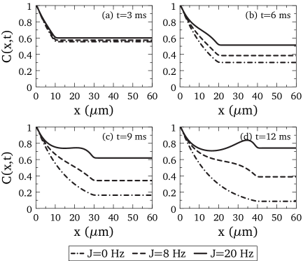
In Fig. 2 we show the correlation functions, as obtained from (14) for different times and coupling $\hbar J=t_{\perp}/\rho$. In particular the four plots correspond to times $t=3,6,9,12\ ms$ and in each plot the values $J=0,8,20\ Hz$ are shown with dotted-dashed, dashed and solid lines respectively. Fig. 2 and the following show the results obtained for the correlation function $C(x,t)$ in (14) computed with $K=\frac{\hbar\pi}{2}\sqrt{\frac{\rho}{mg}}\simeq 30$, $\rho=40\,\mu m^{-1}$ , $\xi_{h}=\hbar/\sqrt{\rho mg}\simeq 0.44\ \mu m$ and $u=\sqrt{\frac{g\rho}{m}}\simeq 1.6\,\mu m/ms$. While the relaxation of the correlations is independent of the tunneling at short times up to a certain extent (see Fig. 2.a), at larger times the effect of tunneling is evident in the long range order (see Fig. 2.b, c and d).

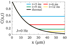
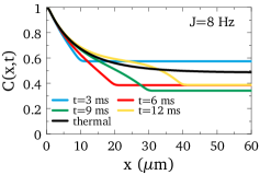
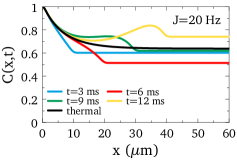
In Fig. 3 we show spatial correlation functions grouped according to the strength of the tunneling $J=0,8,20\ Hz$ and for different times. As in the case without tunneling one sees a light cone in the correlation functions propagating linearly at $x_{c}=2ut$. The decay towards the stationary regime is different, characterized in particular by an oscillating behavior (which is more visible at large $J$). The most important difference between $J=0$ and $J\neq 0$ is a finite plateau value attained by correlation functions in the long time and large distances limit, which is a residue of the coherence induced by the tunneling term.

Figure 3: Spatial correlation functions for different times (coloured lines) compared with the thermal ones at inverse temperature $\beta_{\rm eff}=\frac{4K}{\rho\pi\hbar u}$ (black lines). Blue, red, green and yellow lines correspond respectively to $t=3,6,9,12$ ms. The three plots refer to different values of $J=0,8,20$ Hz.

Indeed, in the limit of large times and distances this correlation function tends to the asymptotic finite value:

$$C(x\to\infty,t\to\infty)=\exp\Big{[}-\frac{1}{4K\lambda}{\mathcal{I}}_{\infty}-\frac{\lambda}{4K}\frac{\sqrt{\pi}}{2}\Big{]}\ ,$$ (17)

with:

$$\begin{array}[]{ll}\displaystyle{\mathcal{I}}_{\infty}=\frac{\pi\,e^{\tilde{m}^{2}}}{2\tilde{m}}\,{\rm Erfc}(\tilde{m})=\frac{1}{\tilde{m}}\Big{[}\frac{\pi}{2}+\mathcal{O}(\tilde{m})\Big{]}\ .\end{array}$$ (18)

In the same semiclassical limit the thermal correlation function reads:

$$C_{\beta}(x)=\exp\Big{[}-\frac{1}{2K}\displaystyle\int_{0}^{\infty}{\rm d}\tilde{p}\,e^{-\tilde{p}^{2}}\frac{1}{\sqrt{\tilde{m}^{2}+\tilde{p}^{2}}}(1-\cos(\tilde{p}\tilde{x}))\,{\rm cotanh}\left(\frac{\tilde{\beta}\,\sqrt{\tilde{m}^{2}+\tilde{p}^{2}}}{2}\right)\Big{]}\ ,$$ (19)

where $\tilde{\beta}=\beta\hbar u/\xi_{h}$ and $\beta$ is the inverse temperature. The thermal correlation function, at temperature $\beta_{\rm eff}=\frac{4K}{\rho\pi\hbar u}$ is shown in Fig. 3 with black solid lines.

In the left panel of Fig. 4 we show the value of correlation functions at $x=40\,\mu m$ as a function of $J$ for different times. On the same Figure we show the thermal equilibrium result at $\beta_{\rm eff}$ which is indistinguishable from the stationary limit of Eq (14).

Figure 4: Left panel: $C(x=40\,\mu m,t)$ for $t=3,5,7,10$ ms shown with blue, red, green and yellow curves respectively . The black curve shows the value $C_{\beta}(x=40\,\mu m)$ given in Eq. (19). The violet curve (which is indistinguishable from the black one at thermal equilibrium) is the asymptotic stationary limit of (14). The inset highlights the region of small $J$ which is more interesting for experiments. Right panel: Correlation functions at large distance as a function of the tunneling strength $J$ for different densities. Blue and red lines refer respectively to times $t=5,10$ ms. Dotted-dashed, dashed and solid lines refer to densities $\rho=30,35,40\ \mu m^{-1}$.

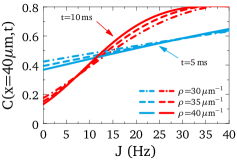
Finally, the right panel of Fig. 4 aims at showing that the results are quite robust in response to variations of the density of about $25\%$.

6 Two-time correlation and response functions

An important way to test the thermalization of the system and eventually measure its temperature is to look at fluctuation-dissipation relations which relate in equilibrium generic two-time correlation and response functions via the temperature of the system cugliandolo2011effective . From this perspective understanding how to access these two-time quantities experimentally in cold atomic experiments is a very interesting question knap2013probing .

In this section we consider the role of the effective temperature defined in (10) at the level of the fluctuation-dissipation relation that involves the correlation and the response function of the relative phase. In order to do this we compute the retarded and the Keldish Green function of the relative phase kamenev2011 where in the following we will denote $[A,B]=AB-BA$ and $\{A,B\}=AB+BA$. In particular we have:

$$\begin{array}[]{ll}\displaystyle G_{R}(x,t;x^{\prime},t^{\prime})&\displaystyle=i\theta(t-t^{\prime})\langle[\theta_{A}(x,t),\theta_{A}(x^{\prime},t^{\prime})]\rangle=\\ \vspace{-0.2cm}\\ &\displaystyle=\theta(t-t^{\prime})\frac{1}{2\pi}\int{\rm d}k\ e^{-ik(x-x^{\prime})-\xi_{h}^{2}k^{2}}\ \frac{\pi u}{\omega_{k}K}\,\sin(\omega_{k}(t-t^{\prime}))\end{array}$$ (20)

Note that this response function does not contain information on the initial state, but only on the final Hamiltonian. Moreover the Keldysh Green function reads:

$$\begin{array}[]{ll}&\displaystyle G_{K}(x,t;x^{\prime},t^{\prime})\displaystyle=\frac{1}{2}\langle\{\theta_{A}(x,t),\theta_{A}(x^{\prime},t^{\prime})\}\rangle=\\ \vspace{-0.2cm}\\ &\displaystyle=\frac{1}{4\pi}\int{\rm d}k\ e^{-ik(x-x^{\prime})-\xi_{h}^{2}k^{2}}\ \Big{[}(\cos\omega_{k}(t-t^{\prime})-\cos\omega_{k}(t+t^{\prime}))\ \left(\frac{\pi u}{\omega_{k}K}\right)^{2}\langle|n_{k}|^{2}\rangle(0)\\ \vspace{-0.2cm}\\ &\displaystyle\qquad\qquad+(\cos\omega_{k}(t-t^{\prime})+\cos\omega_{k}(t+t^{\prime}))\ \langle|\theta_{k}|^{2}\rangle(0)\Big{]}\end{array}$$ (21)

In the stationary limit the Keldysh Green function becomes:

$$\begin{array}[]{ll}\displaystyle G_{K}(x,t;x^{\prime},t^{\prime})=\displaystyle\frac{1}{4\pi}\int{\rm d}k\ e^{-ik(x-x^{\prime})-\xi_{h}^{2}k^{2}}\ \Big{[}\cos\omega_{k}(t-t^{\prime})\ \left(\frac{\pi u}{\omega_{k}K}\right)^{2}\ \frac{\rho}{2}\\ \vspace{-0.2cm}\\ \displaystyle\qquad\qquad\qquad\qquad\qquad\qquad\qquad\qquad\qquad\qquad\qquad\ +\cos\omega_{k}(t-t^{\prime})\ \frac{1}{2\rho}\Big{]}\ .\end{array}$$ (22)

The fluctuation-dissipation theorem (FDT) says that at equilibrium retarded and Keldysh Green function are not independent and satisfy the following relation:

$$G_{K}(\omega)={\rm cotanh}\frac{\omega}{2T}\ (G_{R}(\omega)-G_{A}(\omega))\ .$$ (23)

In the classical limit the FDT simplifies and can be easily written in the time domain:

$$G_{R}(t)=-\frac{\theta(t)}{T}\partial_{t}G_{K}(t)$$ (24)

Therefore by comparing (20) and (22) we note that neglecting in (22) the term $\rho^{-1}$, which corresponds to neglect the initial fluctuation $\langle|\theta_{k}|^{2}\rangle(0)$ with respect to the one in $\rho$ one obtains:

$$\begin{array}[]{ll}\displaystyle\tilde{G}_{K}(x,t;x^{\prime},t^{\prime})&\displaystyle=\frac{1}{4\pi}\int{\rm d}k\ e^{-ik(x-x^{\prime})-\xi_{h}^{2}k^{2}}\cos\omega_{k}(t-t^{\prime})\ \left(\frac{\pi u}{\omega_{k}K}\right)^{2}\ \frac{\rho}{2}\ .\end{array}$$ (25)

and the classical FDT is satisfied with the same $T_{\rm eff}=\frac{\pi u\rho}{4K}$.

7 Discussions

In section 5 we have shown that the presence of a tunneling term, which in our case we treated via a semiclassical approximation has several consequences on the dynamics of the relative phase of the two gases with respect to the uncoupled case.

The transient regime and the way the steady state is reached are in fact quite different than for the case where the two systems are independent. One still sees a light-cone effect LGKRS13 ; CC_2007 ; sotiriadis2010quantum , manifested in Fig. 3 as the length at which correlations show no further space dependences, however after such characteristic (distance-dependent) time the uncoupled gases acquire their stationary value while for $t_{\perp}\neq 0$ the correlations at short distances continue to evolve. This can be interpreted as an effect due to the mass term which implies that not all the quasi-particles travel at the same velocity and after the light-cone which is determined by the fastest excitations, the correlations at short distances still present non stationary effects (as seen in Fig. 3) due to the slow modes. This slowing down in reaching the steady state could make experimentally difficult to observe stationary correlation functions.

As a consequence of the gapped spectrum one also observes in the transient regime the occurrence of oscillations as a function of the space distance which are not obvious if one thinks that the system is completely homogenous and can be interpreted as a non-equilibrium phenomenon.

The other important difference with respect to the uncoupled case is that the correlation functions of the relative phase display long range order and do not decay. This is expected because of the cosine term which favors minima of $\theta$ multiples of $2\pi$. In our approach we only considered the minimum around zero but this effect should be robust if one takes into account solitons between different minima. This result is also in agreement with hofferberth2007non where long time phase coherence in presence of tunneling was also observed.

Despite these differences though, the effective temperature that emerges from simple approximate arguments and by comparing with the asymptotic dynamics does not depend on the tunneling strength and it is the same that was found for the uncoupled case in Gring_Science_2012 ; KISD11 . The thermal correlation functions obtained with this temperature are in fact indistinguishable from the ones obtained after the quench in the stationary limit even if their precise analytical form differs.

These results suggest that in some cases there might be a single temperature that approximate quite accurately at least some observables, even if the detailed dynamics is the one that leads to a generalized Gibbs ensemble with an extensive number of parameters.

However this is probably not a generic property of the post-quench dynamics but a result of how the splitting process creates the initial state. In fact by looking at the energy of the modes (9) one sees that it is possible to discard the dependences on the dispersion relation and thus both the dependencies on $k$ and on the tunneling strength because one can neglect the initial fluctuations of the relative phase. This is a key assumption that allows one to define a $k$-independent temperature, equal for all the modes and one can see that the same approximation allows us to recover the classical FDT in section 6.

In LEGRSKRMGS2014 it was shown in fact that changing the quench protocol drives the system in a state where a single temperature is not sufficient to describe the steady state and instead more Lagrange multipliers are needed to characterize accurately the correlation functions of the interference measurement. The effect of the tunneling on this type of protocol would be very interesting to analyze as in that case one could expect that the dependences on the dispersion relation and therefore on the tunneling strength can modify more sensibly the Lagrange multipliers that account for the constant of motion. Moreover the possibility to measure two-time correlation and response functions as we show in Section 6 for the prethermal state would allow a direct measurement of these Lagrange multipliers foini2016measuring .

As a final remark let us note that in our analysis, as it was done in Gring_Science_2012 we assumed perfect decoupling between the symmetric and the antisymmetric mode. This is the reason way the effective temperature that governs the dynamics is not sensitive to the initial temperature of the system, which is instead expected to appear to characterize the properties of the symmetric mode. The account of the interaction between symmetric and antisymmetric mode and the effect of the tunneling on this type of process and therefore on the final equilibration of the system represents a very interesting perspective.

8 Conclusions

In this work we have studied the relaxation dynamics of two tunnel coupled gases created from the splitting on a single one dimensional gas.

We have seen that the tunneling affects the non stationary dynamics of the system with respect to the independent case leading to oscillations and a general slowing down in reaching the steady state regime.

Differently from the uncoupled case the correlation functions in the steady state show long range coherence, however they are well described by the same effective temperature that was measured in Gring_Science_2012 in absence of tunneling.

The study of this type of protocol is nowadays possible with the current experimental apparatus, and it would be therefore extremely interesting to test these consequences experimentally.

References

- (1) E. Altman. Lecture Notes of the 2012 Les Houches Summer School of Physics ”Strongly Interacting Quantum Systems Out of Equilibrium”, arXiv:1512.00870 (2015).
- (2) B. Rauer, T. Schweigler, T. Langen, J. Schmiedmayer. Proc. Internat. School Phys. Enrico Fermi 191, 485 (2016).
- (3) A. Polkovnikov, K. Sengupta, A. Silva, M. Vengalattore. Rev. Mod. Phys., 83, 863 (2011).
- (4) I. Bloch, J. Dalibard, W. Zwerger. Rev. Mod. Phys., 80, 885 (2008).
- (5) T. Langen, R. Geiger, J. Schmiedmayer. Annu. Rev. Condens. Matter Phys., 6, 201–217 (2014).
- (6) M. Greiner, O. Mandel, T. W. Hänsch, I. Bloch. Nature, 419, 51–54 (2002).
- (7) T. Kinoshita, T. Wenger, D. S. Weiss. Nature, 440, 900–903 (2006).
- (8) M. Gring, M. Kuhnert, T. Langen, T. Kitagawa, B. Rauer, M. Schreitl, I. Mazets, D. A. Smith, E. Demler, J. Schmiedmayer. Science, 337, 1318–1322 (2012).
- (9) T. Langen, S. Erne, R. Geiger, B. Rauer, T. Schweigler, M. Kuhnert, W. Rohringer, I. E. Mazets, T. Gasenzer, J. Schmiedmayer. Science, 348, 207–211 (2015).
- (10) M. Schreiber, S. S. Hodgman, P. Bordia, H. P. Lüschen, M. H. Fischer, R. Vosk, E. Altman, U. Schneider, I. Bloch. Science, 349, 842–845 (2015).
- (11) M. Srednicki. Phys. Rev. E, 50, 888 (1994).
- (12) L. Vidmar, M. Rigol. Journal of Statistical Mechanics: Theory and Experiment, 2016, 064007 (2016).
- (13) P. Calabrese, F. H. Essler, M. Fagotti. Phys. Rev. Lett., 106, 227203 (2011).
- (14) E. Ilievski, J. De Nardis, B. Wouters, J.-S. Caux, F. H. Essler, T. Prosen. Phys. Rev. Lett., 115, 157201 (2015).
- (15) J.-S. Caux, R. M. Konik. Phys. Rev. Lett., 109, 175301 (2012).
- (16) M. A. Cazalilla, A. Iucci, M.-C. Chung. Phys. Rev. E, 85, 011133 (2012).
- (17) G. Mussardo. Phys. Rev. Lett., 111, 100401 (2013).
- (18) J. Berges, S. Borsányi, C. Wetterich. Phys. Rev. Lett., 93, 142002 (2004).
- (19) A. Mitra, T. Giamarchi. Phys. Rev. Lett., 107, 150602 (2011).
- (20) T. Kitagawa, A. Imambekov, J. Schmiedmayer, E. Demler. New Journal of Physics, 13, 073018 (2011).
- (21) D. A. Smith, M. Gring, T. Langen, M. Kuhnert, B. Rauer, R. Geiger, T. Kitagawa, I. Mazets, E. Demler, J. Schmiedmayer. New Journal of Physics, 15, 075011 (2013).
- (22) T. Langen, R. Geiger, M. Kuhnert, B. Rauer, J. Schmiedmayer. Nat. Phys., 9, 607–608 (2013).
- (23) T. Langen, T. Gasenzer, J. Schmiedmayer. J. Stat. Mech. 064009 (2016).
- (24) L. Foini, T. Giamarchi. Phys. Rev. A, 91, 023627 (2015).
- (25) T. Giamarchi. Quantum physics in one dimension. Oxford University Press (2003).
- (26) L. F. Cugliandolo. Journal of Physics A: Mathematical and Theoretical, 44, 483001 (2011).
- (27) M. Knap, A. Kantian, T. Giamarchi, I. Bloch, M. D. Lukin, E. Demler. Phys. Rev. Lett., 111, 147205 (2013).
- (28) A. Kamenev. Field theory of non-equilibrium systems. Cambridge University Press (2011).
- (29) P. Calabrese, J. Cardy. Journal of Statistical Mechanics: Theory and Experiment, 2007, P06008 (2007).
- (30) S. Sotiriadis, J. Cardy. Phys. Rev. B, 81, 134305 (2010).
- (31) S. Hofferberth, I. Lesanovsky, B. Fischer, T. Schumm, J. Schmiedmayer. Nature, 449, 324–327 (2007).
- (32) L. Foini, A. Gambassi, R. Konik, L. F. Cugliandolo. arXiv:1610.00101 (2016).