The Stellar Initial Mass Function in Early-Type Galaxies From Absorption Line Spectroscopy. IV. A Super-Salpeter IMF in the center of NGC 1407 from Non-Parametric Models
Abstract
It is now well-established that the stellar initial mass function (IMF) can be determined from the absorption line spectra of old stellar systems, and this has been used to measure the IMF and its variation across the early-type galaxy population. Previous work focused on measuring the slope of the IMF over one or more stellar mass intervals, implicitly assuming that this is a good description of the IMF and that the IMF has a universal low-mass cutoff. In this work we consider more flexible IMFs, including two-component power-laws with a variable low-mass cutoff and a general non-parametric model. We demonstrate with mock spectra that the detailed shape of the IMF can be accurately recovered as long as the data quality are high (S/N Å-1) and cover a wide wavelength range (). We apply these flexible IMF models to a high S/N spectrum of the center of the massive elliptical galaxy NGC 1407. Fitting the spectrum with non-parametric IMFs, we find that the IMF in the center shows a continuous rise extending toward the hydrogen-burning limit, with a behavior that is well-approximated by a power-law with an index of . These results provide strong evidence for the existence of extreme (super-Salpeter) IMFs in the cores of massive galaxies.
Subject headings:
galaxies: stellar content — galaxies: evolution — stars: luminosity function, mass function1. Introduction
The IMF connects a variety of astrophysical phenomena including star formation, stellar feedback, the relative number of stellar remnants, and heavy element production, and is a critical ingredient in modeling the integrated light from distant galaxies. Precision knowledge of the IMF is essential for understanding the dark matter content within galaxies (e.g., Cappellari et al., 2006) and measuring supermassive black hole masses (e.g., Gebhardt & Thomas, 2009; McConnell et al., 2012). Unfortunately, the IMF is very difficult to measure when individual stars cannot be resolved, owing to the intrinsic faintness of lower main sequence stars relative to the evolved giants (e.g., Conroy & van Dokkum, 2012a).
Nonetheless, in recent years there have been many reported measurements of the IMF in distant galaxies by a variety of techniques, including kinematic analysis, strong lensing, stellar population synthesis, and microlensing (e.g., Cenarro et al., 2003; van Dokkum & Conroy, 2010; Treu et al., 2010; Conroy & van Dokkum, 2012b; Spiniello et al., 2012; Cappellari et al., 2012; La Barbera et al., 2013; Ferreras et al., 2013; Conroy et al., 2013; McDermid et al., 2014; Schechter et al., 2014; Posacki et al., 2015; Lyubenova et al., 2016). The emerging consensus is that the IMF appears to vary systematically from a Milky Way-like IMF (Kroupa, 2001; Chabrier, 2003) at lower galaxy masses to a Salpeter (1955) IMF, or even more bottom-heavy IMF, for the most massive galaxies. This consensus is not without challenges (e.g., Smith, 2014; Smith et al., 2015; Newman et al., 2016).
At the same time, evidence has emerged that the IMF may vary strongly within galaxies, at least at high masses (Martín-Navarro et al., 2015; La Barbera et al., 2016b; van Dokkum et al., 2016; Davis & McDermid, 2017). Not all authors find evidence for radial variation in the IMF (McConnell et al., 2016; Zieleniewski et al., 2016), though it is not clear if the different conclusions are due to small sample sizes or the analysis techniques. The existence of strong IMF gradients implies that direct comparison between different techniques requires careful consideration of aperture effects.
When inferring the IMF from the depth of stellar absorption lines, all analyses to date have focused on parameterized IMFs, e.g., a single power-law or a broken power-law, with a fixed low-mass cutoff. Recently, Spiniello et al. (2015) and Lyubenova et al. (2016) have combined stellar population and dynamical constraints for individual galaxies in order to place stronger constraints on the shape of the IMF.
Here we go one step further and attempt to constrain the general form of the IMF directly from the absorption line spectra of old stellar systems. We consider several models, including a two-part power-law with a variable low-mass cutoff and a general non-parametric IMF (see also Dries et al., 2016, who explored the ability to reconstruct the IMF from mock data). Our goals are 1) to assess what is measurable from absorption line spectra in the idealized limit of perfect models, and 2) to reconstruct from real data the IMF under different assumptions and assess how the derived mass-to-light ratio depends on these assumptions.
2. Models & Spectral Fitting
2.1. Overview
Our approach to constructing stellar population models follows Conroy & van Dokkum (2012a, CvD12a), with several important updates. First and foremost, the models now span a wider range of ages and metallicities, with ages extending from Gyr and metallicities from [Z/H]=-1.5 to [Z/H]=+0.25. Second, we now adopt the MIST stellar isochrones (Choi et al., 2016) which obviate the need to stitch together various isochrone databases as done in CvD12a. Third, we have obtained IRTF NIR spectra for 283 stars from the MILES spectral library (Sánchez-Blázquez et al., 2006), providing continuous spectral coverage from for stars with well-known stellar parameters over a wide range in metallicity. The details of the new library are presented in Villaume et al. (2016). In addition to the new library, we have created a polynomial spectral interpolator that provides stellar spectra for arbitrary , , and [Z/H], the details of which are presented in Villaume et al. (2016). We include the library of M dwarfs from Mann et al. (2015) to more fully population the cool dwarf regime for the purposes of constraining the interpolator. Fourth, the theoretical response functions, which are computed from the ATLAS and SYNTHE model atmosphere and spectrum synthesis package (Kurucz, 1970, 1993), have been recomputed with updated atomic and molecular data and for stellar parameters covering the full age and metallicity range of the new models. The element response functions are then tabulated as a function of age and metallicity assuming a Kroupa IMF. We have checked that the derived mass-to-light ratios do not change substantially if the response functions are instead computed with a Salpeter IMF (but see La Barbera et al., 2016a, for an example where this choice may affect the NIR Na i lines at ).
The methodology for fitting models to data is similar to the approach described in Conroy & van Dokkum (2012b) and Conroy et al. (2014). Namely, we employ a Markov chain Monte Carlo algorithm (Foreman-Mackey et al., 2013) in order to sample the posteriors of the following parameters: redshift and velocity dispersion, a two component star formation history (two bursts with free ages and relative mass contribution), the overall metallicity, [Z/H], 18 individual elements (though many are irrelevant from the standpoint of the IMF, e.g., Sr and Ba), the strengths of five emission line groups (including the Balmer lines which are assumed to have relative line strengths determined by Case B recombination), a hot star component with that can vary from 8,000 K to 30,000 K, and IMF parameters described below. In addition, we fit for several data-related systematics, including a a multiplicative factor applied to the observed errors, a sky emission spectrum that is used to increase the errors specifically around sky lines, and a telluric absorption spectrum, whose overall strength is a free parameter. The parameters affecting the observed errors are given a penalty in the likelihood calculation in order to discourage the fitter from inflating the errors to be arbitrarily high. Mismatch between the observed and model continuum shape is treated by fitting a polynomial to the ratio of the model and data. This polynomial is recomputed for each likelihood evaluation.
2.2. IMF Models
In all models in this work the IMF slope above is assumed to have the Salpeter (1955) value of 2.35, the upper mass limit is and stellar remnants are included in the final mass calculation following Conroy et al. (2009). We explore three options for the parameterization of the IMF. The first option has two free parameters, and , corresponding to the logarithmic slope of the IMF () over the mass intervals and . In this first option the low-mass cutoff is fixed to . Grids of models were pre-tabulated with ranging from . Option one is the model IMF adopted in all of our previous work (e.g., Conroy & van Dokkum, 2012b; Conroy et al., 2013; van Dokkum et al., 2016). Option two is the same as option one except that the low-mass cutoff, is a free parameter. Pre-computed grids were made for .
Option three is a non-parametric111The term “non-parametric” is a something of a misnomer, as there are many parameters in the model (one for each bin), in addition to the choice of intra-bin behavior. In the present case, the term is meant to indicate that the IMF is not required to follow an analytic (parametric) equation. IMF. We have pre-computed what we call “partial SSPs” (simple stellar populations), which are SSPs computed within a bin in stellar mass of width from , and for the lowest mass bin. One must still choose the IMF weighting within each bin; for this work we adopt a Salpeter IMF intra-bin weighting because direct measurements of the IMF are consistent with Salpeter-like slopes, at least for (Bastian et al., 2010). We will also consider Kroupa-like intra-bin weighting to explore the impact of this assumption. In a more general treatment the intra-bin weighting would be an additional free parameter. In order to keep the number of free parameters manageable, we only explicitly include five parameters in the model for the bins starting at 0.08, 0.3, 0.5, 0.7 and 0.9. The weights for the other bins are computed via linear interpolation between the fitted bins. We emphasize that all bins contribute to the final model and hence to the minimization. The overall normalization has no effect on the spectrum nor the mass-to-light ratio, so to further decrease the number of free parameters we have fixed the weight for the highest-mass bin to 1.0. This leaves four free parameters for the non-parametric IMF option. Finally, we adopt a regularization procedure in order to ensure that the final IMF is smooth. The prior requires that the logarithmic slope of the IMF between two mass bins cannot change from negative to positive when moving from lower to higher masses (e.g., if the logarithmic slope in the bin is negative while the slope in the bin is positive, then the prior on that point in parameter space is set to 0.0).
The choice of model priors can be an important, often hidden assumption when fitting models to data, especially when parameters are poorly constrained (e.g., when the S/N of the data is low). In our case we have adopted uniform, wide priors in all parameters, where the range is in most cases only limited by the range of the pre-computed grids. For the high S/N regime explored in this paper, the priors play a minimal role. The variables governing the parameterized IMF models (options one and two) are allowed to vary over the full range offered in the pre-computed grids. For the case of the non-parametric IMF, the models are parameterized with weights, such that the IMF within a bin is . In these units a Salpeter IMF would have . The priors on these weights are flat in log space from -5.0 to +3.0 (subject to the regularization condition mentioned above).
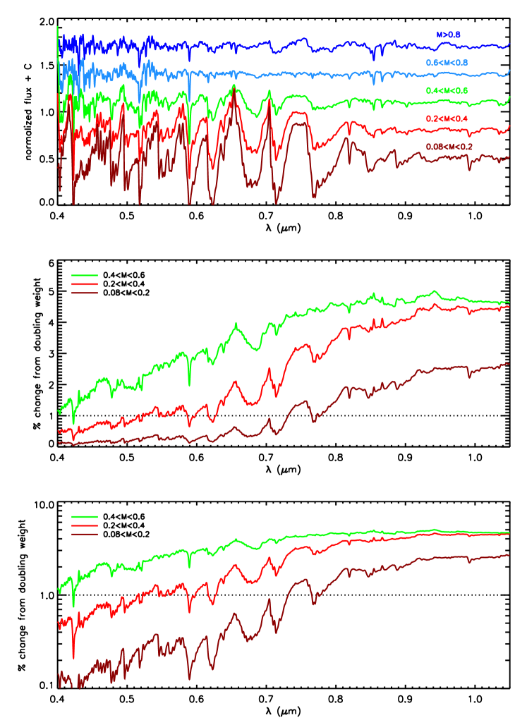
Figure 1 presents an overview of the partial SSPs that are the building blocks for the non-parametric IMF models. We have grouped together the partial SSPs in mass bins wide, except for the lowest mass bin, for display purposes. The models shown in this figure were computed assuming [Z/H]=0.0 and an age of 13.5 Gyr, though the qualitative trends are generic. The top panel shows the models normalized by a polynomial in order to zoom in on the trends in the absorption lines with mass. The sensitivity of various features to surface gravity and temperature is strong throughout the entire wavelength range (see also CvD12a). The middle and bottom panels show the percentage change to the full SSP model when doubling the weight assigned to each mass bin, assuming a fiducial Salpeter IMF. Unsurprisingly, the lowest mass bins contribute very little flux in the blue, which is why the NIR spectral range is critical for robust constraints on the low mass IMF.
3. Mock Tests
In this section we explore the extent to which the IMF and band mass-to-light ratio, , can be recovered from mock data (in this paper mass-to-light ratios are quoted in units of ). We create mock spectra with a fixed S/N per Å over the wavelength range and a velocity dispersion of (these characteristics were chosen to be similar to the observations discussed in the following section). In all cases the age is fixed to 10 Gyr, the metallicity is [Z/H]=0.0, with solar-scaled abundance patterns, and the various nuisance parameters are set to zero. The only component that varies is the functional form of the IMF. The input mock spectra are constructed with a parametric IMF with a single logarithmic slope over the mass range where is the lower-mass cutoff. Note that this IMF parameterization is not, in general, contained within the model space for the non-parametric models. This only occurs in the case where and equals one of the mass boundaries for the non-parametric IMF; in this case the parametric and non-parametric models exactly agree because the intra-bin weighting for the latter models assumes . These mock spectra therefore offer a strong test of the ability of the non-parametric models to recover general IMF behavior.
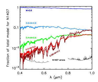
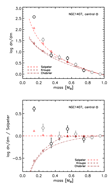
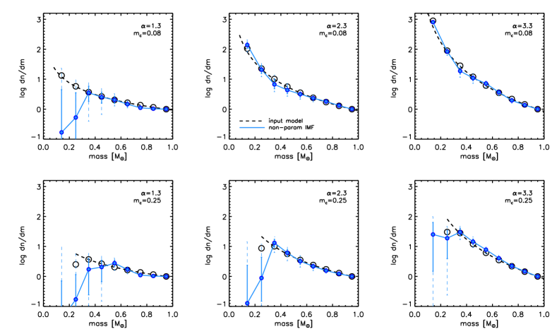
Figure 2 shows the inferred non-parametric IMFs for mock spectra with six input IMFs. All of the mock spectra were computed with S/N Å-1. The best-fits (solid symbols) are compared to the input IMFs (dashed lines) and the input IMF averaged over the same mass bins as the non-parametric IMF models (open symbols). Overall, the recovery of the input IMF with the non-parametric models is remarkable. In the case of the shallow input IMF () the contribution to the total flux from the lowest mass bins is very small, and so the non-parametric IMF recovery is biased low, a consequence of the very wide priors on the individual IMF weights. However, the very fact that these low-mass bins contribute very little to the light and so are difficult to constrain also implies that they contribute little to the mass. As an example, the bias shown in the upper left panel results in only a 16% bias in the recovered
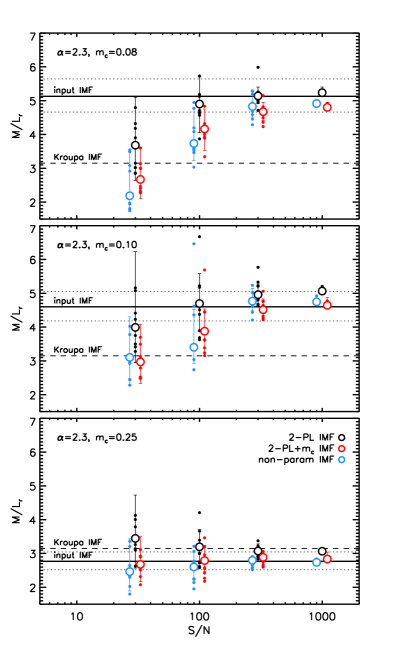
We explore the ratios explicitly in Figure 3. This figure shows the best-fit as a function of S/N for mock spectra constructed with an IMF with a Salpeter slope and a low-mass cutoff of (top panel), (middle panel) and (bottom panel). Each mock spectrum was fit three times for the three IMF options described in Section 2. For each S/N ten mock spectra were created with identical parameters and independent realizations of the noise. Results from fitting each realization are shown as small symbols and the median is shown as large open symbols. Error bars denote the median confidence limits and should be interpreted as the “typical” error on a single measurement. The for a Kroupa (2001) IMF is indicated by the dashed lines.
Although the overall agreement is good, it is clear from this figure that there can be important biases in the recovered depending on the S/N, the adopted functional form of the fitted IMF, and the input IMF. Results at S/N tend to be biased low when the low-mass cutoff is . This occurs because the data are not of sufficient quality to constrain the low-mass behavior, and so the posteriors tend toward the priors, which in our setup favors low mass-to-light ratios. For S/N Å-1 the results are never biased by more than 10% for the input models explored here.
Another important conclusion to draw from Figure 3 is that the IMF ‘mis-match’ parameter, , is a good summary statistic when S/N Å-1, irrespective of the detailed IMF shape (although we have not tested single power-law models in this paper). This is important and suggests that the parameter is a reliable, compact metric for IMF measurements.
The conclusion from this section is that the full, non-parametric IMF can be robustly inferred from the spectrum, given sufficiently high S/N data. For the specific case of a 10 Gyr solar metallicity population with a dispersion of the requirement is S/N Å-1 if the IMF is Salpeter-like and extends to ; a shallower IMF and/or one with a higher-mass cutoff will have less severe S/N limitations. This requirement will depend, at a minimum, on the velocity dispersion, age, and metallicity of the population, and the wavelength range of the data. Attempts to measure the IMF from fitting absorption line spectra should therefore include tests with mock observations to assess potential biases in the derived parameters.
4. Results
We now turn to applying these models to observations. Here we focus on the massive elliptical galaxy NGC 1407 ( Mpc, kpc). We recently observed this galaxy with the LRIS instrument on the Keck I telescope, obtaining high S/N spectra as a function of radius. The data extend beyond although the S/N in the red drops below 200 at . Details of the observing strategy and data reduction can be found in van Dokkum et al. (2016). Here we fit the data over the wavelength intervals , , and . The gap at is due to the dichroic and grating tilt, while the gap at reflects the fact that atmospheric absorption strongly contaminates that spectral region. We focus on the central region within . The detailed stellar population gradients, including and IMF gradients (based on simpler IMF models), are presented in van Dokkum et al. (2016).
We begin with Figure 4, where we show the best-fitting model for NGC 1407. The model is displayed as fractional contributions to the total model spectrum for stars in five mass intervals. For comparison we also include the fractional errors for the observed spectrum of NGC 1407. Not surprisingly, the most massive stars dominate the flux, contributing % of the flux over the entire wavelength range. It is noteworthy that each remaining mass bin interval contributes at least 4% per pixel over wavelength intervals of at least 1000Å. Compared to the fractional errors on the data, which are at the level of , it is clear that each mass interval is well constrained by the data.
Figure 5 shows the best-fit non-parametric IMF for the center of NGC 1407. The top panel shows the IMF while the bottom panel shows the IMF divided by a Salpeter IMF () in order to highlight the behavior at lower masses. For comparison we also show Salpeter (1955), Kroupa (2001), and Chabrier (2003) IMFs (dashed and dot-dashed lines) and those IMFs averaged over the non-parametric IMF mass bins (diamonds). Recall that only four bins are explicitly free parameters (those with bins starting at 0.08, 0.3, 0.5, and ); the bin is fixed to 1.0 and the weights for the four remaining bins are determined by linear interpolation between the other bins.
This figure shows that the central region of NGC 1407 prefers an IMF considerably heavier at low masses than Salpeter, by a factor of in the lowest mass bin. The inferred mass-to-light ratio is , or a factor of two (three) times higher than the mass-to-light ratio for a Salpeter (Kroupa) IMF (errors on reflect the 16% and 84% confidence limits). It is remarkable that the lowest mass bin is so well-constrained (although not surprising in light of Figure 1).
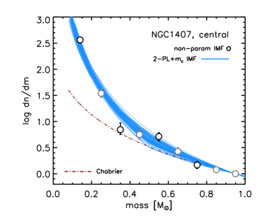
We have also fit the spectrum of NGC 1407 assuming a three parameter IMF model (two-part power-law and a variable low-mass cutoff) to explore the sensitivity of the derived mass-to-light ratio to the assumed IMF with real data. The comparison of this model to the non-parametric IMF is shown in Figure 6. In this figure we draw 100 random samples from the posteriors of the three parameter IMF. The agreement is impressive and lends further weight to the robustness of the derived IMF. The best-fit IMF parameters in this case are , , and . The inferred for the three parameter model agrees very well with the non-parametric IMF-based value. Moreover, the low-mass cutoff is constrained to be lower than at 97.5% CL, confirming that the IMF for the central region of NGC 1407 remains steep toward the hydrogen-burning limit. All of the other derived parameters (age, metallicity, abundance pattern, etc.) agree to within 0.01 dex or better when comparing results for the two IMF parameterizations.
We have tested the impact of several model assumptions on these results. Recall that the element response functions were tabulated assuming a Kroupa IMF. We have re-fit the central spectrum of NGC 1407 with response functions tabulated assuming a Salpeter IMF in order to assess the impact of this assumption (see also La Barbera et al., 2016a). The best-fit in this case is higher by 17%, suggesting that the IMF derived with the fiducial response functions is slightly lower than the true value. Moreover, the Na i feature is slightly better fit when using response functions constructed with a Salpeter IMF, even though the best-fit [Na/Fe] abundance is virtually identical in the two cases. In the future we will explore this issue in greater depth and consider options for treating the IMF in the response functions in a self-consistent manner.
We have also explored the sensitivity of these results to the intra-bin weighting used to compute the partial SSPs. Our default models employ Salpeter intra-bin weights. We have created an additional set of models with Kroupa-like intra-bin weighting (power-law indices of for and for ). The resulting IMF constraints are nearly identical to the default model, and the inferred mass-to-light ratio is , also nearly identical to the mass-to-light ratio inferred with the default models. We conclude that our results are insensitive to the choice of intra-bin weighting, at least within the Kroupa-Salpeter range.
5. Discussion
In Paper III of this series (van Dokkum et al., 2016) we explored stellar population gradients in six galaxies, including NGC 1407. Using simpler IMF models (a two-part power-law with a fixed low-mass cutoff) we found strong IMF gradients in all six galaxies. The extreme IMF in the center of NGC 1407 reported here, derived with more flexible IMF models, is evidently a phenomenon confined to the inner regions.
Several distinct analytical models have been proposed to explain the origin of the IMF and its dependence on the properties of the interstellar medium and/or the galaxy as a whole. The model proposed by Krumholz (2011) argues that the characteristic fragmentation mass in a molecular cloud is governed by radiation released by the collapsing protostar. This process produces a weak relation between the characteristic stellar mass and the pressure of the surrounding gas such that high pressure environments produce lower characteristic masses. Hennebelle & Chabrier (2008), Hopkins (2012), and Chabrier et al. (2014) argue that the IMF emerges from the combined effects of gravity and lognormal density fluctuations in a turbulent medium (with the important assumption that the ratio between core and stellar mass is constant). Recently, Guszejnov et al. (2016) combined these ideas by considering a model that includes both gravito-turbulent fragmentation and stellar radiation feedback.
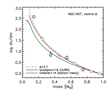
In Figure 7 we compare several of these semi-analytic models to our recovered IMF for the central region of NGC 1407. We include the model for extreme starburst conditions from Chabrier et al. (2014, Case 3), and the ULRIG model from Guszejnov et al. (2016). For comparison we also include a power-law IMF of the form , and note that in the formalism of Chabrier et al. the most extreme IMFs saturate at an index of . The agreement between the observations and the Chabrier et al. model is remarkable given that there was no fine tuning in the model parameters.
The derived IMF for the central region of NGC 1407 is very steep, which means that the total stellar mass is sensitive to the adopted low-mass IMF cutoff. In our non-parametric analysis, the lowest-mass bin covers the range , so we cannot make strong statements regarding the cutoff mass, only that it must extend below . When computing mass-to-light ratios we have assumed that the lowest mass bin extends to . To illustrate the sensitivity of the total mass to the cutoff, for a single power-law with , the mass-to-light ratio is 70% higher if the cutoff is compared to .
It is therefore critical to understand which physical processes set the low-mass cutoff, and how we might hope to constrain the location of the cutoff in early-type galaxies. Chabrier et al. (2014) argue, based on calculations presented in Masunaga & Inutsuka (1999), that the minimum mass for fragmentation may be much higher in early-type galaxies compared to the Milky Way, owing to the higher temperatures, densities, and opacities in the former. For reasonable conditions, the minimum mass could be comparable to the hydrogen-burning limit, implying a sharp truncation in the IMF near .
A promising path forward to constrain the low-mass cutoff in early-type galaxies is the joint modeling of stellar populations, dynamics, and/or gravitational lensing (e.g., Barnabè et al., 2013; Spiniello et al., 2015). In this approach, the stellar population analysis constrains the IMF over the stellar range (as in this work), and the dynamics and/or lensing probe the integral of the IMF down to the low-mass cutoff, irrespective of whether that cutoff is in the stellar or sub-stellar regime. With this approach one must still make an assumption regarding the mass in stellar remnants, i.e., the shape of the IMF above , if one wants to constrain the low-mass cutoff. Early work along these lines by Barnabè et al. (2013) and Spiniello et al. (2015) appears promising, and suggests that the cutoff in massive early-type galaxies is indeed near .
In this work we used updated stellar population models to constrain the detailed shape of the IMF over the range in the center of the massive early-type galaxy NGC 1407. The IMF in the galaxy core is very steep, consistent with down to the hydrogen-burning limit. Such a steep IMF is also consistent with the IMF predicted for extreme starburst conditions from Chabrier et al. (2014). These results demonstrate that it is possible to directly probe the “bottom” of the IMF from absorption line spectra of old stellar systems.
References
- Barnabè et al. (2013) Barnabè, M., Spiniello, C., Koopmans, L. V. E., et al. 2013, MNRAS, 436, 253
- Bastian et al. (2010) Bastian, N., Covey, K. R., & Meyer, M. R. 2010, ARA&A, 48, 339
- Cappellari et al. (2006) Cappellari, M. et al. 2006, MNRAS, 366, 1126
- Cappellari et al. (2012) —. 2012, Nature, 484, 485
- Cenarro et al. (2003) Cenarro, A. J., Gorgas, J., Vazdekis, A., Cardiel, N., & Peletier, R. F. 2003, MNRAS, 339, L12
- Chabrier (2003) Chabrier, G. 2003, PASP, 115, 763
- Chabrier et al. (2014) Chabrier, G., Hennebelle, P., & Charlot, S. 2014, ApJ, 796, 75
- Choi et al. (2016) Choi, J., Dotter, A., Conroy, C., et al. 2016, ApJ, 823, 102
- Conroy et al. (2013) Conroy, C., Dutton, A. A., Graves, G. J., Mendel, J. T., & van Dokkum, P. G. 2013, ApJ, 776, L26
- Conroy et al. (2014) Conroy, C., Graves, G. J., & van Dokkum, P. G. 2014, ApJ, 780, 33
- Conroy et al. (2009) Conroy, C., Gunn, J. E., & White, M. 2009, ApJ, 699, 486
- Conroy & van Dokkum (2012a) Conroy, C. & van Dokkum, P. 2012a, ApJ, 747, 69
- Conroy & van Dokkum (2012b) Conroy, C. & van Dokkum, P. G. 2012b, ApJ, 760, 71
- Davis & McDermid (2017) Davis, T. A. & McDermid, R. M. 2017, MNRAS, 464, 453
- Dries et al. (2016) Dries, M., Trager, S. C., & Koopmans, L. V. E. 2016, MNRAS, 463, 886
- Ferreras et al. (2013) Ferreras, I., La Barbera, F., de la Rosa, I. G., et al. 2013, MNRAS, 429, L15
- Foreman-Mackey et al. (2013) Foreman-Mackey, D., Hogg, D. W., Lang, D., & Goodman, J. 2013, PASP, 125, 306
- Gebhardt & Thomas (2009) Gebhardt, K. & Thomas, J. 2009, ApJ, 700, 1690
- Guszejnov et al. (2016) Guszejnov, D., Krumholz, M. R., & Hopkins, P. F. 2016, MNRAS, 458, 673
- Hennebelle & Chabrier (2008) Hennebelle, P. & Chabrier, G. 2008, ApJ, 684, 395
- Hopkins (2012) Hopkins, P. F. 2012, MNRAS, 423, 2037
- Kroupa (2001) Kroupa, P. 2001, MNRAS, 322, 231
- Krumholz (2011) Krumholz, M. R. 2011, ApJ, 743, 110
- Kurucz (1970) Kurucz, R. L. 1970, SAO Special Report, 309
- Kurucz (1993) —. 1993, SYNTHE spectrum synthesis programs and line data, ed. Kurucz, R. L.
- La Barbera et al. (2013) La Barbera, F., Ferreras, I., Vazdekis, A., et al. 2013, MNRAS, 433, 3017
- La Barbera et al. (2016a) La Barbera, F., Vazdekis, A., Ferreras, I., et al. 2016a, ArXiv:1610.03853
- La Barbera et al. (2016b) —. 2016b, MNRAS, 457, 1468
- Lyubenova et al. (2016) Lyubenova, M., Martín-Navarro, I., van de Ven, G., Falcón-Barroso, J., Galbany, L., et al. 2016, MNRAS, 463, 3220
- Mann et al. (2015) Mann, A. W., Feiden, G. A., Gaidos, E., Boyajian, T., & von Braun, K. 2015, ApJ, 804, 64
- Martín-Navarro et al. (2015) Martín-Navarro, I., La Barbera, F., Vazdekis, A., Ferré-Mateu, A., Trujillo, I., & Beasley, M. A. 2015, MNRAS, 451, 1081
- Masunaga & Inutsuka (1999) Masunaga, H. & Inutsuka, S.-i. 1999, ApJ, 510, 822
- McConnell et al. (2016) McConnell, N. J., Lu, J. R., & Mann, A. W. 2016, ApJ, 821, 39
- McConnell et al. (2012) McConnell, N. J., Ma, C.-P., Murphy, J. D., et al. 2012, ApJ, 756, 179
- McDermid et al. (2014) McDermid, R. M., Cappellari, M., Alatalo, K., et al. 2014, ApJ, 792, L37
- Newman et al. (2016) Newman, A. et al. 2016, submitted
- Posacki et al. (2015) Posacki, S., Cappellari, M., Treu, T., Pellegrini, S., & Ciotti, L. 2015, MNRAS, 446, 493
- Salpeter (1955) Salpeter, E. E. 1955, ApJ, 121, 161
- Sánchez-Blázquez et al. (2006) Sánchez-Blázquez, P., Peletier, R. F., Jiménez-Vicente, J., Cardiel, N., Cenarro, A. J., Falcón-Barroso, J., Gorgas, J., Selam, S., & Vazdekis, A. 2006, MNRAS, 371, 703
- Schechter et al. (2014) Schechter, P. L., Pooley, D., Blackburne, J. A., & Wambsganss, J. 2014, ApJ, 793, 96
- Smith (2014) Smith, R. J. 2014, MNRAS, 443, L69
- Smith et al. (2015) Smith, R. J., Lucey, J. R., & Conroy, C. 2015, MNRAS, 449, 3441
- Spiniello et al. (2015) Spiniello, C., Barnabè, M., Koopmans, L. V. E., & Trager, S. C. 2015, MNRAS, 452, L21
- Spiniello et al. (2012) Spiniello, C., Trager, S. C., Koopmans, L. V. E., & Chen, Y. P. 2012, ApJ, 753, L32
- Treu et al. (2010) Treu, T., Auger, M. W., Koopmans, L. V. E., Gavazzi, R., Marshall, P. J., & Bolton, A. S. 2010, ApJ, 709, 1195
- van Dokkum et al. (2016) van Dokkum, P. et al. 2016, submitted
- van Dokkum & Conroy (2010) van Dokkum, P. G. & Conroy, C. 2010, Nature, 468, 940
- Villaume et al. (2016) Villaume, A., Conroy, C., et al. 2016, in preparation
- Zieleniewski et al. (2016) Zieleniewski, S., Houghton, R. C. W., Thatte, N., Davies, R. L., & Vaughan, S. P. 2016, ArXiv:1611.01095