Multi-level Monte Carlo acceleration of computations on multi-layer materials with random defects

Abstract

We propose a Multi-level Monte Carlo technique to accelerate Monte Carlo sampling for approximation of properties of materials with random defects. The computational efficiency is investigated on test problems given by tight-binding models of a single layer of graphene or of $\mathrm{MoS}_{2}$ where the integrated electron density of states per unit area is taken as a representative quantity of interest. For the chosen test problems the multi-level Monte Carlo estimators significantly reduce the computational time of standard Monte Carlo estimators to obtain a given accuracy.

1 Introduction

The aim of this study is to develop non-intrusive numerical techniques for approximating properties of layered heterostructures with impurities in random locations.

The goal is to apply these techniques on models developed and used for layered heterostructures such as tight-binding models for transition-metal dichalcogenides (TMDC). The numerical techniques are not in themselves restricted to tight-binding models, but can be combined with more computationally intensive and accurate models when such are called for. For the purpose of testing and calibrating the algorithms we use two simple tight-binding models of materials with honeycomb lattices. The first is of graphene, where individual atoms at random locations are “removed” from the tight-binding model without changing the positions of the surrounding atoms. This example can be viewed as a rough approximation of a graphene sheet where hydrogen atoms are attached to randomly distributed carbon atoms in the sheet without mechanically deforming the sheet. We also use a tight-binding model of a single layer of the TMDC $\mathrm{MoS}_{2}$; in this model $\mathrm{S}$ atoms are similarly removed.

Characteristically we wish to compute material properties which, in the unperturbed case of a periodically repeating fundamental cell, can be obtained by computing the band structure of the material over the first Brillouin zone associated with the fundamental cell. Here we test the approach on computations of the integrated electronic density of states per unit area of the material, which can be computed from the band structure and is a common quantity of interest in such computations. This is interesting on its own, and also serves as a test case for the more computationally demanding problem of computing the electric conductivity by the Kubo-Greenwood formula. This tensor depends both on the energies of the band structure and on the corresponding eigenstates.

We assume that the random perturbations result in an ergodic random field. Random perturbations of the studied material break the periodicity, which is used when computing the band structure and quantities depending upon it. A common approach in this case is to extend the fundamental cell of the unperturbed material along the primitive lattice vectors. In the test case this means extending the fundamental cell of the honeycomb lattice by some integer factors $N_{1}$ and $N_{2}$ along its primitive lattice vectors. Random perturbations are introduced in this “super cell” of the fundamental cell, which is then periodically extended to cover the whole plane. The band structure can now be computed, but at a much higher cost, increasing with the size of the super cell. Finally, in theory, the size of the super cell is allowed to go to infinity to obtain the limit of random perturbations without periodicity. In the remainder of this paper we will let $N_{1}=N_{2}=N$.

The discrete random perturbations in our test examples only allow a finite number of outcomes for each finite super cell. Indeed, if the super cell is small enough it is efficient to compute the quantity of interest for all possible combinations of perturbations, which with the known probability of each outcome gives a complete description of the random quantity of interest. This exhaustive approach can not be extended to large super cells where our true interest lies in the case of a randomly perturbed material; neither can it be applied where the perturbations vary continuously. We are left with approximate methods. For low densities of impurities in particular, homogenisation or perturbation around the solution of the problem without impurities can be used. Here we will instead study Monte Carlo methods to estimate the expected value of the quantity of interest, which is a random variable for a finite size super cell. The main advantage of Monte Carlo type methods is in their simplicity; they are non-intrusive methods in the sense that they approximate the expected value of the desired quantity by the average over several independent outcomes of the random perturbations, and each outcome can be computed using any existing code capable of taking the perturbed configuration as an input.

Our goal is to use so called Multilevel Monte Carlo methods to reduce the computational cost of standard Monte Carlo sampling while retaining the same accuracy. The key point here is to systematically generate control variates to an expensive, accurate, numerical approximation of a random sample. With a suitable choice of control variates fewer samples on the most expensive and most accurate approximation level are needed and the total computational cost to reach a given accuracy can be reduced. In Section 2 we will describe Monte Carlo and Multilevel Monte Carlo estimators for the test problem and discuss the numerical complexity assuming simplified models of the approximation properties and computational cost of the underlying computational method. In Section 3 we describe our tight-binding test problems and explain how to generate control variates for Multilevel Monte Carlo in this context. Finally, in Section 4 we show numerical experiments which illustrate the efficiency of the multilevel approach on the given test problems.

2 Monte Carlo and MultiLevel Monte Carlo

By Monte Carlo methods here we simply mean methods where the expected value of a random variable is approximated by the sample average over several, usually independent, outcomes of the random variable. In the present context this means that we generate a number of outcomes of the random perturbations of the materials model on the super cell and then compute the quantity of interest for each outcome individually by separate calls to the underlying computational physics code. In this spirit we want to restrict ourselves to Monte Carlo techniques that do not strongly depend on the particular qualities of our test problem; for example we do not in this discussion optimize our methods given test problem by utilizing the fact that only a finite number of perturbations are possible for each finite super cell.

2.1 Monte Carlo complexity

The quantity of interest in the test problem applied in Section 3, which is an integrated density of states, is a deterministic quantity in the infinite volume limit, $|V|\sim N^{d}\to\infty$; that is the variance goes to zero as the size of the super cell goes to infinity. Does this mean that we should use only one sample of the random perturbations in the material?

We can answer the above question by estimating the rate at which the variance of our quantity of interest goes to zero as the super cell size, $N$, increases, and compare this to the rate at which the expected value of the quantity converges and the rate at which the computational work grows. Let $Q$ be the exact value, in this case deterministic, of the quantity we wish to approximate, let $Q_{N}$ be the random variable of the same quantity computed on a finite super cell of size $N$ with random perturbations, and let ${\mathbb{E}\mspace{-2.0mu}\left[Q_{N}\right]}$ and $\mathrm{Var}(Q_{N})$ denote the expected value and the variance of $Q_{N}$, respectively. Assume the following models for the above quantities:

(1a) the finite $$N Q-{\mathbb{E}\mspace{-2.0mu}\left[Q_{N}\right]} \propto N^{-W},$$ bias,

(1b) the variance, $$\mathrm{Var}(Q_{N}) \propto N^{-S},$$

(1c) the cost per sample, $$\mathtt{cost} \propto N^{C},$$

for some positive constants $W$, $S$, $C$. Assume, for now, that the number of samples, $M\to\infty$, and approximate the expected value ${\mathbb{E}\mspace{-2.0mu}\left[Q_{N}\right]}$ by the estimator

(2) $$\mathcal{A}_{\mathrm{MC}}(M) =\frac{1}{M}\sum_{m=1}^{M}Q_{N}(m),$$

where $Q_{N}(m)$ denotes the $m$:th independent sample of $Q_{N}$. Then by the Central Limit Theorem we can justify approximating the suitably rescaled statistical error of our Monte Carlo estimator by the Standard Normal random variable, $N(0,1)$, which allows us to state the following error constraints. To make the total error in our quantity of interest approximately TOL with high probability, we require that the bias is approximately $(1-\Theta)\textrm{TOL}$ for some $\Theta\in(0,1)$ and the variance of our Monte Carlo estimator is approximately $\frac{1}{C_{\alpha}}(\Theta\textrm{TOL})^{2}$ where the confidence parameter $C_{\alpha}$ is chosen for a Standard Normal random variable. That is

$$N^{-W} \approx(1-\Theta)\textrm{TOL},$$

$$\frac{1}{M}N^{-S} \approx\frac{1}{C_{\alpha}}(\Theta\textrm{TOL})^{2}.$$

Minimizing the total work, proportional to $N^{C}$, with respect to $\Theta$ while satisfying the two constraints leads to the simple expression for the splitting parameter

$$0<\Theta =\frac{1}{1+\frac{C-S}{W}}<1,$$

provided that the cost of generating samples grow faster than the variance of the sampled random variables decrease, i.e. $C>S$. Furthermore, the optimal number of samples becomes $M\propto\textrm{TOL}^{-(2-S/W)}$ which, as long as $S<2W$, goes to infinity as $\textrm{TOL}\to 0$. With the work per sample assumed to be $N^{C}$ and with $N^{-W}\approx(1-\Theta)\textrm{TOL}$ the total work for a Monte Carlo method is then approximately proportional to

(3) $$\mathtt{Work}_{\mathtt{MC}}(\textrm{TOL}) \propto\textrm{TOL}^{-(2+\frac{C-S}{W})}.$$

A method using a fixed number of samples must take $N\propto\textrm{TOL}^{-2/S}$, assuming that $S<2W$, giving the asymptotic complexity

(4) $$\mathtt{Work}_{\mathtt{FS}}(\textrm{TOL}) \propto\textrm{TOL}^{-\frac{2C}{S}}.$$

Thus, the Monte Carlo complexity (3) is an improvement as long as $C>S$.

Qualitatively the above argument tells us that for small error tolerance it is more computationally efficient to use several samples on a smaller super cell than to use a larger super cell with only one sample of the random perturbations. For quantitative predictions on the optimal choice we may use a sequence of increasing super cell sizes to empirically estimate the parameters in the models for how the bias and variance decays with $N$ and how the work grows with $N$. From these estimates we can decide how to optimally choose the number of samples versus the size of the super cell.

2.2 Multilevel Monte Carlo as an acceleration of standard Monte Carlo

Assume that the models (1) hold approximately for large enough $N$ and that parameters, $W$, $S$, and $C$, have been empirically or theoretically estimated and found to be such that it is more efficient to use Monte Carlo sampling than one single sample on a very large super cell. In this situation we want to use Monte Carlo methods to approximate the expected value of a quantity which in turn has a bias due to a method parameter; in this case we assume most importantly by the size given test problem of the super cell, $N$. Over the past decade so called Multilevel Monte Carlo (MLMC) method has become an increasingly popular systematic technique for accelerating such Monte Carlo methods. They can be traced back to Heinrich et al. [7, 8] where they were introduced for parametric integration, and were independently proposed by Giles [3] in a form closer to the one in this paper. Following [3] the methods have typically been applied to problems where each sample of a standard Monte Carlo sample is obtained by the solution of a discretization based numerical approximation to a stochastic differential equation or a partial differential equation with random data. This technique depends on the possibility of using cheaper approximations of the quantity to be evaluated for each random sample as control variates for more accurate approximations; see [4]. For example, in a discretization based numerical method characterized by a mesh size, $h$, with known convergence as $h\to 0$, a solution using a larger step size $2h$ can be used as a control variate to a solution using a step size $h$ which have been chosen to make the bias sufficiently small. A good use of control variates means that fewer samples on the accurate, most expensive, scale can be used, while samples on less accurate and less costly scales are introduced to compensate.

In the present context the artificially finite super cell size introduces a bias which only vanishes in the limit as $N\to\infty$. We also assume that among the parameters in the numerical approximation $N$ dominates the computational cost as our tolerated error $\textrm{TOL}\to 0$. It is then natural to consider using approximate values of our quantity of interest based on smaller super cell sizes as control variates to the more accurate approximations computed on large super cells. Assume, for now, that for $N_{\ell}=c2^{\ell}$, with $c,\ell\in\mathsf{Z}_{+}$, in addition to the approximate quantity of interest $Q_{\ell}$ on super cell size $N$ we can construct control variates $Q_{\ell}^{CV}$ such that

(5a) $${\mathbb{E}\mspace{-2.0mu}\left[Q_{\ell}^{CV}\right]} ={\mathbb{E}\mspace{-2.0mu}\left[Q_{\ell-1}\right]},$$

(5b) $$\mathrm{Var}(Q_{\ell}-Q_{\ell}^{CV}) \propto N^{-D},$$

for some $D>S$, and the cost of sampling the control variate is small compared to sampling the original quantity of interest; at most a constant fraction smaller than one say, so that (1c) holds for generating the pair $(Q_{\ell},Q_{\ell}^{CV})$. Following the standard MLMC approach the estimator (2) is now replaced by

(6) $$\mathcal{A}_{\mathrm{MLMC}} =\frac{1}{M_{1}}\sum_{m=1}^{M_{1}}Q_{1}(\omega_{1,m})+\sum_{\ell=2}^{L}\frac{1}{M_{\ell}}\sum_{m=1}^{M_{\ell}}\left(Q_{\ell}(\omega_{\ell,m})-Q_{\ell}^{CV}(\omega_{\ell,m})\right),$$

where $N_{\ell}=c2^{\ell}$ for $\ell=1,2,\dots,L$, and $M_{\ell}$ denotes the positive integer number of samples used on size $N_{\ell}$; by $\omega_{\ell,m}$ we denote the $m$:th independent identically distributed outcome of the random impurities on a super cell of size $N_{\ell}$. Note that while we assume independence between all terms of the sums in (6), the difference $Q_{\ell}(\omega_{\ell,m})-Q_{\ell}^{CV}(\omega_{\ell,m})$ is computed using the same outcome of the random perturbation but two different approximations of $Q$.

Taking the expected value, the sum over $\ell$ in the definition (6) telescopes by assumption (5a) so that $\mathcal{A}_{\mathrm{MLMC}}$ is an unbiased estimator of ${\mathbb{E}\mspace{-2.0mu}\left[Q_{L}\right]}$. Furthermore, by independence of the outcomes $\omega_{\ell,m}$,

$$Var{\left(\mathcal{A}_{\mathrm{MLMC}}\right)} =\frac{1}{M_{1}}\mathrm{Var}(Q_{1})+\sum_{\ell=2}^{L}\frac{1}{M_{\ell}}\mathrm{Var}(Q_{\ell}-Q_{\ell}^{CV}),$$

where the variances are assumed approximated by (1b) and (5b). Similarly to the standard Monte Carlo case we require that the sum of the bias and the statistical error of the estimator sum up to a specified error tolerance, TOL. Denote by $W_{\ell}$ the work, as modeled by (1c), of computing one sample on level $\ell$, that is $Q_{1}$, for $\ell=1$, or $Q_{\ell}-Q_{\ell}^{CV}$, for $\ell=2,\dots,L$. Also let $V_{\ell}$ denote the corresponding variances predicted by models (1b), for $\ell=1$, and (5b), for $\ell=2,\dots,L$. A straightforward minimization of the computational work model with respect to the number of samples on each level leads to

(7) $$M_{\ell} =\left(\frac{C_{\alpha}}{\theta\textrm{TOL}}\right)^{2}\sqrt{\frac{V_{\ell}}{W_{\ell}}}\sum_{k=1}^{L}\sqrt{W_{k}V_{k}}, \ell=1,\dots,L$$ for

in terms of general work estimates, $\{W_{\ell}\}_{\ell=1}^{L}$, and variance estimates, $\{V_{\ell}\}_{\ell=1}^{L}$; see for example [6]. Here the number of levels, $L$, depends on TOL through the constraint on the finite $N$ bias.

Further minimizing the predicted work of generating $\mathcal{A}_{\mathrm{MLMC}}$ with respect to the splitting between bias and statistical error, the model of the computational work becomes

(8) $$\mathtt{Work}_{\mathtt{MLMC}}(\textrm{TOL}) \propto\textrm{TOL}^{-(2+\frac{C-D}{W})}.$$

This improves on the computational work of a standard Monte Carlo method as long as $D>S$, that is as long as $\mathrm{Var}(Q_{\ell}-Q_{\ell}^{CV})$ decays at a higher rate in $N_{\ell}$ than $\mathrm{Var}(Q_{\ell})$. The applicability of MLMC techniques depends on finding control variates satisfying this condition. We will describe how to generate such control variates in Section 3.3.

3 Tight-binding model with random defects

In our test problems the target is to compute the integrated density of states in tight-binding models of a single-layer material with honeycomb lattices. The first example is a simple nearest neighbor tight-binding model of graphene, which provides us with a well controlled, and comparatively inexpensive, test setting where we can study the algorithms before turning to new materials. The second example is a tight-binding model of one layer of $\mathrm{MoS}_{2}$.

3.1 Materials model without defects

In a tight-binding model of a periodically repeating material, we take a given numbering of the atoms in the fundamental cell of the periodic material and identify periodic images of the atoms. Using values for hopping and on-site energies obtained for example by parameter fitting to more accurate density functional theory results we construct a Hamiltonian matrix, $H(k)$, and an overlap matrix, $S(k)$, leading to a generalized eigenvalue problem

(9) $$H(k)u =\epsilon S(k)u.$$

Our quantities of interest will depend on the solutions to (9) for each point $k$ in the Brillouin zone.

A tight-binding model for graphene

Here we use a nearest neighbor tight-binding model of a single-layer graphene sheet from Chapter 2.3.1, “$\pi$ Bands of Two-Dimensional Graphite”, in [9].

In this tight-binding model, including only the $\pi$ energy bands, the generalized eigenvalue problem (9) is defined by

(10a) $$H_{mm}(k) =\epsilon_{2p}$$

(10b) $$H_{mn}(k) =t_{mn}\exp{(ik\cdot R_{mn})}$$

(10c) $$S_{mm}(k) =1$$

(10d) $$S_{mn}(k) =s_{mn}\exp{(ik\cdot R_{mn})}$$

where $R_{mn}$ is the vector from atom position $m$ to $n$ in the honeycomb lattice. In the nearest neighbor interactions the parameters $t_{mn}$ and $s_{mn}$ are 0 unless atoms $m$ and $n$ are nearest neighbors and $t_{mn}=\langle\phi_{m}|\mathcal{H}|\phi_{n}\rangle=t$ and $s_{mn}=\langle\phi_{m},\phi_{n}\rangle=s$, independent of $m$ and $n$, otherwise. The numerical values were taken from [9] to be

$$\epsilon_{2p} =0\,\mathrm{eV} t =-3.033\,\mathrm{eV} s =0.129\,\mathrm{eV}$$

which gives the Fermi level $\epsilon_{F}=0\,\mathrm{eV}$.

The fundamental cell of the honeycomb lattice of the graphene sheet has two atoms, call them $A$ and $B$, so that $H(k)$ and $S(k)$ are 2-by-2 matrices where by the periodic structure the only non-diagonal elements $H_{AB}(k)=H_{BA}(k)^{\star}$ are obtained by summing (10b) over the three nearest neighbor directions; similarly $S_{AB}(k)=S_{BA}(k)^{\star}$ is obtained from (10d).

A tight-binding model of $\mathrm{MoS}_{2}$

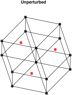
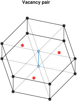
In an ideal single layer $\mathrm{MoS}_{2}$, the projection of the atom positions on the plane forms a honeycomb lattice, just as for graphene. This time the two types of lattice positions, $A$ and $B$, are occupied by an $\mathrm{Mo}$-atom and a pair of $\mathrm{S}$-atoms, separated in the direction perpendicular to the plane of the $\mathrm{MoS}_{2}$ layer; see Figure 2.

In this example we take the tight-binding model of a monolayer TMDC material from Section IV, equations (4)–(10), in [2], and the parameters for $\mathrm{MoS}_{2}$ in Table VII of the same paper. This model includes 11 bands and interactions up to selected third-neighbor couplings which together define the Hamiltonian $H(k)$; the overlap matrix $S(k)$ is the identity matrix.

3.2 Materials model with defects

We now consider the case when individual atom locations in the infinite sheet of the honeycomb lattice are “removed” from the tight-binding model. In the graphene case, we view this as a rough approximation to hydrogen atoms attaching to the corresponding carbon atoms and thus changing the electron interactions without mechanically deforming the sheet. Still in the graphene case, the locations of the removed atom locations are random, and it is assumed that each atom location is removed, with probability $p$, $0<p<1$, independently of all other locations. A vacancy is modeled by removing all rows and columns corresponding to interactions involving this lattice site from the tight-binding Hamiltonian matrix, $H(k)$, and overlap matrix, $S(k)$.

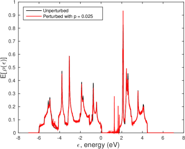
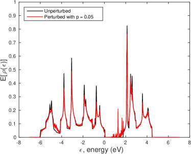
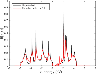
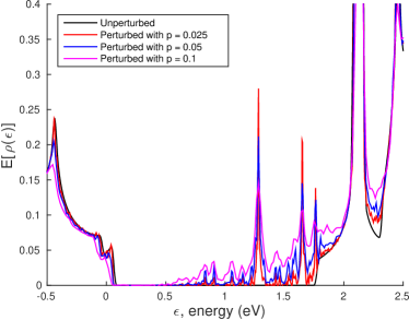
In a simplified test of perturbations of the $\mathrm{MoS}_{2}$ layer, in order to keep the example similar to the graphene model, we let the permutations remove pairs of $\mathrm{S}$ atoms located at randomly sites, instead of individual S atoms; see Figure 1. Any such pair of $\mathrm{S}$ atoms is removed with probability $p$ independently of all other pairs. No Mo atoms are removed. The numerical tests include three different probabilities $p=0.025$, 0.05, and 0.1. Such a vacancy pair is modeled by removing from the tight-binding Hamiltonian matrix, $H(k)$, all rows and columns corresponding to Wannier orbitals involving this particular pair of $\mathrm{S}$ atoms.

Ideally the atom locations should be chosen independently of each other on the entire infinite sheet, but as described above, this is approximated by taking a large super cell where the impurities are distributed randomly; this super cell and its impurities are then repeated periodically to create an infinite sheet. We seek the limit as the size of the super cell goes to infinity, and commit an approximation error by keeping it finite.

Figure 1: $\mathrm{MoS_{2}}$: (Left) Unperturbed MoS2 (Right) Perturbed by vacancy pair.

3.3 Control Variates for an MLMC Approach

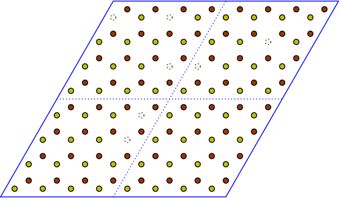
The MLMC approach to accelerate the standard Monte Carlo sampling introduced in Section 2 rests on the possibility to automatically generate control variates for the random variable whose expected value we wish to approximate. The control variates must be cheaper to sample than the target random variable while still being strongly correlated to the target. In our randomly perturbed tight-binding model the dominating factor in the computational cost of generating one sample is the size of the finite super cell, $N$. It is thus natural to try control variates on smaller super cells which, for any given outcome of random impurities, resemble the larger super cell. Assume for example that $N$ is divisible by 2. We can divide a large super cell into four parts where each part retains the impurities of the larger super cell as illustrated in Figure 2 and then extend each part periodically to an infinite sheet. The quantity of interest computed on each one of the four parts will be correlated to that computed on the larger super cell, and we can take the arithmetic mean of the four parts as our control variate.

Figure 2: Control variate idea. In the 8-by-8 super cell on the top the brown and yellow circles illustrate atom sites of type “A” and “B”, respectively. Seven circles have been removed indicating that the corresponding sites have been replaced by vacancies. This is one random outcome of the impurities on a rather small super cell. The larger super cell has been divided into four corners which all inherit the impurities of the corresponding part of the larger super cell. These four smaller super cells are themselves extended periodically to the entire plane; the quantity of interest is computed on all four of them, and the arithmetic mean is used as a control variate for the quantity computed on the larger super cell.

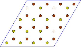
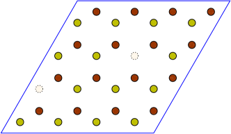
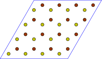
More generally, let $\mathcal{F_{\ell}}$ denote the $\ell$:th supercell in the MLMC hierarchy, $P(\ell)$ denote the number of atom sites in $\mathcal{F_{\ell}}$, and $X=(x_{1},\dots,x_{P(\ell)})$ be the coordinates of the $P(\ell)$ atom sites. We represent a partition of $\mathcal{F_{\ell}}$ into $R$ subdomains by the function $\Phi_{\ell}:\mathcal{F_{\ell}}\to\{1,\dots,R\}$. We then define the control variate

$$Q_{\ell}^{CV}(\omega;\mathcal{F_{\ell}}) =\frac{1}{R}\sum_{r=1}^{R}Q_{\ell-1}\left(\omega;\Phi_{\ell}^{-1}(r)\right),$$

where $\omega$ denotes a the outcome of the random perturbation on level $\ell$ and $Q_{\ell-1}\left(\omega;\Phi_{\ell}^{-1}(r)\right)$ denotes the quantity of interest computed on the subproblem restricted to $\Phi_{\ell}^{-1}(r)$. We require that the partition is chosen so that $Q_{\ell-1}\left(\dot{;}\Phi_{\ell}^{-1}(r)\right)$ are i.i.d. random variables for independent outcomes of the random perturbations to guarantee that condition (5a) is satisfied. In the specific case of the tight-binding models in Section 3.2, this restricted subproblem involves solving generalized eigenvalue problems (9) with matrices $H(k)$ and $S(k)$ satisfying the periodicity condition on the new subdomains.

This systematic way of generating control variates in a multilevel approach can be naturally extended to other geometries, for example an infinite nano ribbon. The random impurities could then model either impurities along the edge following some given distribution or again atoms binding to the surface of the ribbon in random locations. The requirement (5a) will be satisfied as long as the super cell in this quasi 1D problem is divided along the direction of the ribbon.

4 Numerical Tests

Here we empirically investigate whether the proposed control variates satisfy the conditions under which MLMC improves on the computational complexity of standard Monte Carlo sampling.

4.1 Quantities of Interest

The physical quantity to approximate from our computational model in the test case is the integrated electronic density of states of the material. For a periodic material, before we let the artificial finite size of the super cell go to infinity, this property depends on the bandstructure computed over the first Brillouin zone.

4.2 Numerical approximation of bandstructure

The first Brillouin zone associated with the fundamental cell of the honeycomb lattice is a regular hexagon. For the unperturbed material, it is by symmetry sufficient to consider a rhombus which constitutes one third of the Brillouin zone. This rhombus is here uniformly divided into $K_{1}$ by $K_{2}$ rhombi, with discretization points, $k_{mn}$, in the corners of the rhombi. For each $k_{mn}$ the generalized eigenvalue problem (9) is solved numerically using Matlab’s full eigenvalue solver “eig”.

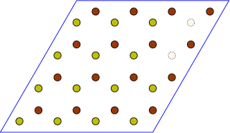
Note that for a nearest neighbor tight-binding model the matrices of the generalized eigenvalue problem are sparse; see Figure 3 for examples with $N=8$. As $N$ grows larger one must take advantage of the sparsity in the eigenvalue computations. However, more complex tight-binding models will be less sparse, and in more accurate density functional theory computations the corresponding problems become non-linear and very much more complex to solve.

Figure 3: Sparsity structure of an outcome of the matrix $H$ with $N=8$ for the graphene (left) and $\mathrm{MoS}_{2}$ (right) models.

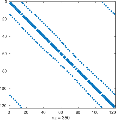
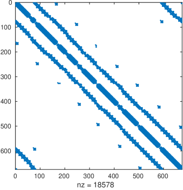
For a super cell where the fundamental cell has been extended by an integer factor $N$ along both primitive lattice vectors, the first Brillouin zone is still a regular hexagon, rescaled by the factor $1/N$. Perturbations in random atom locations in the periodically repeating super cell break the symmetry which allowed us to compute the bandstructure on a third of the Brillouin zone. Hence the bandstructure is computed on three rhombi which combined make up the Brillouin zone. In all the numerical examples we used $K_{1}=K_{2}=K$, where in turn the resolution in the Brillouin zone was held constant as $N$ increased; that is $NK=\mathtt{constant}$. In the graphene example $K=64/N$ and in the $\mathrm{MoS}_{2}$ example $K=128/N$.

4.3 Numerical approximation of the integrated density of states

The quantity of interest in the present test is the expected value of the integrated density of states. The electronic density of states per unit area of the two-dimensional material, $\rho(\epsilon)$ at energy $\epsilon$, is defined as the limit when $\Delta\epsilon\to 0$ of the total number of eigenstates (normalized by area) with energies between $\epsilon$ and $\epsilon+\Delta\epsilon$. The integrated density of states in turn is $I(\epsilon)=\int_{x=-\infty}^{\epsilon}\rho(x)\,dx$. Let $\mathcal{F}$ and $\mathcal{B}$ denote the fundamental cell and the first Brillouin zone respectively, and let $E_{n}:\mathcal{B}\to\mathsf{R}$ denote the $n$:th band in the bandstructure, that is $E_{n}(k)$ is the $n$:th smallest eigenvalue of the algebraic eigenvalue problem (9) for $k\in\mathcal{B}$. Then

(11) $$I(\epsilon) =\frac{1}{|\mathcal{F}|}\sum_{n}\frac{1}{|\mathcal{B}|}\int_{\mathcal{B}}\chi_{\left\{\cdot<\epsilon\right\}}(E_{n}(k))\,dk,$$

where $\chi_{\left\{\cdot<\epsilon\right\}}$ is the indicator function on the semi-infinite interval $(-\infty,\epsilon)$ and $|\cdot|$ denotes area.

The bands in (11) are, in the case of the unperturbed graphene sheet on its fundamental cell, $n\in\{1,2\}$ and for an $N$-by-$N$ super cell without vacancies $n\in\{1,2,\dots,2N^{2}\}$. Similarly for the $\mathrm{MoS}_{2}$ model $n\in\{1,2,\dots,11\}$ and $n\in\{1,2,\dots,11N^{2}\}$, respectively.

For each sampled outcome (11) is approximated from the computed discretization of the bandstructure, $\{E_{n}(k_{lm})\}$ in two steps. First, $E_{n}(k)$ is approximated by $\overline{E_{n}}(k)=E_{n}(k_{lm})$ where $k_{lm}$ is the discretization point closest to $k$. Then, the indicator function (11) is approximated by a smoothed, Lipschitz continuous, step function

(12) $$\chi_{\left\{\cdot<\epsilon\right\}}(E) \approx g\left(\frac{E-\epsilon}{\delta}\right),$$

satisfying

$$g(x) =1, \text{if $x\leq-1$},$$

$$g(x) =0, \text{if $x\geq 1$},$$

$$\int_{-1}^{1}x^{q}\left(\chi_{\left\{\cdot<0\right\}}(x)-g(x)\right)\,dx =0, q=0,1$$ for .

This smoothing, using $\delta\propto\textrm{TOL}$ where TOL is the desired accuracy, is needed when MLMC methods are used to compute distribution functions of random variables; see [5] for an analysis of MLMC methods in this case. Similar smoothing strategies are also used in the computational physics community. Finally, $I$, is approximated in a uniform discretization $\epsilon_{0}<\epsilon_{1}<\dots<\epsilon_{M}$ of an interval containing the range of computed energies.

The expected value of the integrated density of states is approximated by Monte Carlo or MLMC sample averages. From the expected value of the integrated density of states the density of states may be estimated by numerical differentiation.

4.4 Numerical Results

The following numerical results are intended to show whether an MLMC approach can accelerate computations of the quantity of interest in the test problems; in particular it is important to see that the control variates suggested in Section 3.3 improves on the rate of convergence of the variance of the samples, so that $D>S$ in the models (1) and (5).

A Tight-binding model of graphene

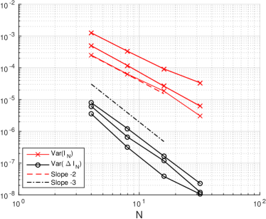
An empirical investigation of how the quantities used in the complexity analysis of Section 2 behave for the tight-binding model of graphene using modest super cell sizes, up to a 32-by-32 extension of the fundamental cell of the honeycomb lattice, containing 2048 atom locations. The results show that in this example the sample variance of the quantity of interest, $Q_{\ell}$, measured in discrete norms, decays approximately as $N^{-2}$, and the sample variance of $Q_{\ell}-Q_{\ell}^{CV}$ decays faster, approximately as $N^{-3}$. The computational cost per sample is nearly independent of $N$ for the first few sample points, where the generalized eigenvalue problems only involve a few unknowns, and starts to grow only around $N=8$. Between $N=16$ and $N=32$ the rate of growth is approximately 4; see also Figure 5 for the $\mathrm{MoS}_{2}$ case. In the notation of Section 2, the empirical estimates of the parameters are

(13) $$W \approx 1.5, S =2, D =3, C =4.$$

Since $D>S$ the asymptotic complexity of an MLMC algorithm should be better than that of a standard Monte Carlo method. We expect an improvement on the computational work using MLMC as soon as $N>=32$ here. The smallest control variate worth including in the MLMC estimator (6) is $N=16$ since samples on smaller super cell sizes are nearly as expensive.

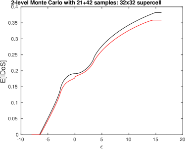
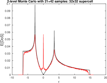
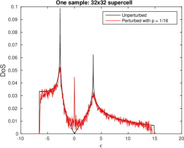
Following the observation above, a 2-level Monte Carlo estimator based on super cell sizes $N=32$ and $N=16$ for the control variate is shown in Figure 4. Here the 2-level estimator used 21 samples on the larger super cell size, $N=32$, and 42 samples on the smaller size, $N=16$. For comparison an additional 21 independent samples on $N=32$ were generated and a single level estimator based on 42 samples computed. The variance of the two estimators are nearly of the same magnitude as desired, while the cost of the 2-level estimator was $61\%$ of that of the standard Monte Carlo estimator. It can be seen most clearly from the density of states, computed by numerical differentiation, that it is crucial to control the statistical error even on a super cell of this size. The two plots of the density of states computed either from the 2-level Monte Carlo estimator or from a single outcome of random impurities use the same resolution in the energy; in the latter case noise hides all detail.

Note that the work ratio between MLMC and standard Monte Carlo will not remain constant at around $61\%$ as we aim for more accurate solutions, provided that the empirical complexity and convergence estimates extrapolate to larger $N$ with the present rates. The next example will illustrate this.

The tight-binding model of $\mathrm{MoS}_{2}$

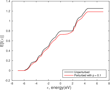
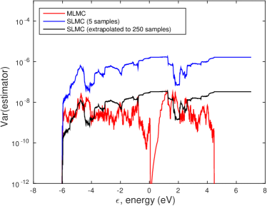
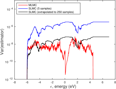
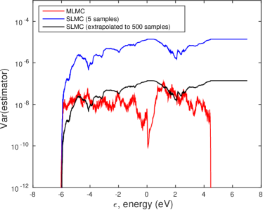
Here, using the parameters in Table 1, we again observe the values in (13) for the parameters in the convergence and work models. By the estimates of Section 2, we expect the computation time of standard Monte Carlo to grow as $\textrm{TOL}^{-(2+\frac{C-S}{W})}\approx\textrm{TOL}^{-10/3}$ while that of MLMC to grow as $\textrm{TOL}^{-(2+\frac{C-D}{W})}\approx\textrm{TOL}^{-8/3}$ as $\textrm{TOL}\to 0$. For the fixed accuracy of the numerical results here, we estimate that using a standard Monte Carlo estimator the work required to obtain a variance in $I(\epsilon)$ comparable to that observed in the MLMC estimator would be one order of magnitude larger; see Table 2.

In the numerical tests of the $\mathrm{MoS}_{2}$ we made use of the fact that in the total number of possible permutations is finite for each finite super cell size. For a sufficiently small super cell, the number of possible combinations is small enough to compute the quantity of interest on all of them, taking symmetries into account, and then by combinatorial means obtain the probabilities of all possible outcomes for a complete description of the statistics. This was done for the smallest $2\times 2$ super cell for all values of $p$. For $p=0.025$ and 0.05 we also took advantage of the finite space of possible outcomes of the perturbations by identifying identical samples of the random perturbations beforehand and avoiding repeating them. This leads to substantial computational savings on the still rather small $4\times 4$ and $8\times 8$ super cells.

In these numerical tests we started with rough estimates of the parameters in the models (1) and (5) to determine a sequence of samples using (7). The resulting values of $M_{\ell}$ are rough approximations of the optimal choices. An alternative approach is to use an algorithm to estimate the parameters during the computation and adaptively choose the number of samples; see [1].

Figure 4: A bi-level Monte Carlo approximation of the integrated density of states on a 32-by-32 super cell with probability of any atom location being removed from the tight-binding model $p=0.0625$, denoted $Q_{\ell}$ below.
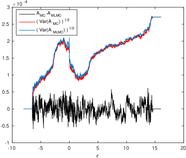
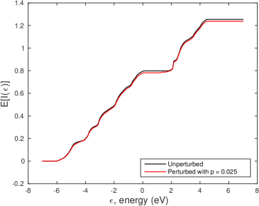
(Top left) Black curve shows the difference between a 42 sample standard Monte Carlo estimate of $Q_{\ell}$ and a bi-level Monte Carlo estimator using 21 samples of $Q_{\ell}$ and 42 of its control variate $Q_{\ell}^{CV}$, obtained at $61\%$ of the cost of the single level. The standard deviations of the two estimators are of the same order.
(Top right) The bi-level Monte Carlo estimate of ${\mathbb{E}\mspace{-2.0mu}\left[Q_{\ell}\right]}$ together with the unperturbed.
(Bottom left) Approximation of the density of states obtained by numerical differentiation of the bi-level Monte Carlo estimate above.
(Bottom right) Approximation of the density of states based on only one sample and the same resolution in the energy.

$p=0.025$
Level	$N$	$M$	$NK$	$\delta$	$\Delta\epsilon$	time (h)
1	2	Exhaustive	128	0.01	3.9$\times 10^{-3}$	0.33
2	4	2072	128	0.01	3.9$\times 10^{-3}$	13.4
3	8	564	128	0.01	3.9$\times 10^{-3}$	92.7
4	16	76	128	0.01	3.9$\times 10^{-3}$	137
5	32	5	128	0.01	3.9$\times 10^{-3}$	128
					total time	372
$p=0.05$
Level	$N$	$M$	$NK$	$\delta$	$\Delta\epsilon$	time (h)
1	2	Exhaustive	128	0.01	7.8$\times 10^{-3}$	0.33
2	4	2450	128	0.01	7.8$\times 10^{-3}$	30
3	8	474	128	0.01	7.8$\times 10^{-3}$	126
4	16	77	128	0.01	7.8$\times 10^{-3}$	150
5	32	5	128	0.01	7.8$\times 10^{-3}$	124
					total time	430
$p=0.1$
Level	$N$	$M$	$NK$	$\delta$	$\Delta\epsilon$	time (h)
1	2	Exhaustive	128	0.01	15.6$\times 10^{-3}$	0.37
2	4	2072	128	0.01	15.6$\times 10^{-3}$	283
3	8	564	128	0.01	15.6$\times 10^{-3}$	161
4	16	76	128	0.01	15.6$\times 10^{-3}$	139
5	32	5	128	0.01	15.6$\times 10^{-3}$	129
					total time	702

Table 1: Parameters in the MLMC estimator in Figure 6 and the computational times spent on each level of the MLMC hierarchy as well as the total time. Here, $N$ is the super cell size, $M$ is the number of samples, $K$ controls the discretization of the Brillouin zone as in Section 4.2, $\delta$ is the smoothing parameter in (12), and $\Delta\epsilon$ is the step size in the numerical differentiation in the post processing step used to get the density of states in Figure 8.
The computational times are wall times for one core on multi-core processors, where one sample was running on each core. The computations with $p=0.025$ and $p=0.05$ did not repeat computations on identical outcomes of the random perturbation leading to significant computational savings on levels 1 and 2 where the probability of repeated outcomes is high.

$p$	$W$	$S$	$D$	$C$	$AC_{\mathtt{FS}}$	$AC_{\mathtt{SLMC}}$	$AC_{\mathtt{MLMC}}$	$R$
0.025	3/2	2	3	4	4	3+1/3	2+2/3	0.06
0.05	3/2	2	3	4	4	3+1/3	2+2/3	0.07
0.1	3/2	2	3	4	4	3+1/3	2+2/3	0.06

Table 2: The parameters, $W$, $S$, $D$, and $C$, in the models (1) and (5) estimated from the numerical experiment on $\mathrm{MoS}_{2}$; compare Figure 5. Included are also the corresponding estimated asymptotic complexities $\mathtt{Work}\propto\textrm{TOL}^{-AC}$ in the work estimates (4), (3) and (8). Finally, $R$ denotes the ratio between the observed computational time of the MLMC method and the estimated time for a standard Monte Carlo method to obtain approximately the same variance; see Figure 7.

Figure 5: $\mathrm{MoS_{2}}$: (Left) The sample variance of the integrated density of states per unit area, $I_{N}(\epsilon)$, using a super cell of size $N\times N$ and the sample variance of the difference, $\Delta I_{N}(\epsilon)=I_{N}(\epsilon)-I_{N/2}(\epsilon)$, for the three vacancy probabilities in Table 1. Shown here is the arithmetic mean of the quantities over the discretization points in the interval $-6\mathrm{eV}<\epsilon<4\mathrm{eV}$ and the sample variance was computed using the samples in the MLMC estimators. In particular the sample variance on the largest super cell is based on only five samples. The experimentally observed convergence rates are approximately $S=2$ and $D=3$.
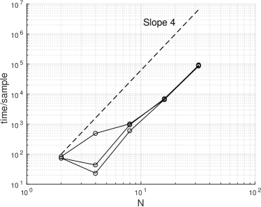
(Right) Wall time per sample in the simulations where each sample was run on a single core of a multi core processor. An eigenvalue problem for a full matrix of side $\propto N^{2}$ were solved for every discretization point of the Brillouin zone, giving the cost per eigenvalue solve $\propto N^{6}$ for large enough $N$. Since the number of such discretization points were chosen to decrease as $N^{-2}$, the observed time per sample is approximately $\propto N^{4}$; see Section 4.2.

Figure 6: $\mathrm{MoS_{2}}$: MLMC approximations of the expected integrated density of states, $I(\epsilon)$, on a 32-by-32 super cell with the probability, $p$, of any $\mathrm{S}$ atom pair being removed from the tight-binding model taking the values $p=0.025,~{}0.05~{},0.1$ respectively. The integrated density of states for unperturbed material is shown for comparison. The MLMC estimators were computed using the parameters in Table 1.

Figure 7: $\mathrm{MoS_{2}}$: Estimates of the pointwise variance of the MLMC estimators of Figure 6 are compared with the corresponding variance estimates when only the five samples on the 32-by-32 super cell were used in a single level Monte Carlo (SLMC) estimator. Also included are rescaled versions of the SLMC variances chosen so that they are comparable to those of the MLMC estimators in the interesting range $1\mathrm{eV}<\epsilon<2\mathrm{eV}$, which contains the upper part of the band gap of the unperturbed material. This gives rough estimates of how many samples the SLMC estimators would need to match the error of the MLMC estimators; see Table 1.

Figure 8: $\mathrm{MoS_{2}}$: The density of states per unit area, $\rho(\epsilon)$, computed by numerical differentiation of the MLMC estimator in Figure 6. The step sizes used in the numerical differentiation are given in Table 1. The bottom right sub figure shows the density of states for all vacancy probabilities, $p$, together with that of the unperturbed material in an interval containing the bandgap of the unperturbed material.

5 Conclusions and future work

We have studied Monte Carlo and MLMC sampling methods for quantities of interest depending on the band structure of quasi 2D materials with random impurities. We have presented a method of constructing control variates for the quantities of interest by subdividing super cells into parts and using the arithmetic mean of the quantity on the periodically extended parts. Using two tight-binding models on a honeycomb lattice, we have empirically estimated the convergence rates of the finite super cell bias, the variance on a finite super cell, and the variance of the difference between a finite super cell sample and its control variate, and found that for these test cases an MLMC approach will be more computationally efficient than a standard Monte Carlo approach, which is in turn more efficient than using one single sample on a larger super cell.

In the graphene test problem with a 32-by-32 super cell, a 2-level Monte Carlo estimator of the same variance as a standard Monte Carlo estimator was obtained at $61\%$ of the computational time of the latter. This ratio should improve for a true Multilevel Monte Carlo estimator as the size of the super cell increases. Indeed, in an $\mathrm{MoS}_{2}$ test problem, an MLMC estimator with five super cell sizes ending with a 32-by-32 super cell, the estimated computational savings were at least one order of magnitude. More precisely, based on the estimated convergence rates and costs, and on the asymptotic complexity estimates, the work of an MLMC estimator to meet accuracy TOL in the quantity of interest in the test problem is asymptotically proportional to $\textrm{TOL}^{-8/3}$ while the work of a standard Monte Carlo estimator with the same accuracy grows like $\textrm{TOL}^{-10/3}$ as $\textrm{TOL}\to 0$.

Future work includes applying the MLMC approach for more demanding quantities of interest, such as the conductivity tensor, other geometries such as nano ribbons and bilayer heterostructures, studying more realistic distribution of vacancies in the tight-binding model of $\mathrm{MoS}_{2}$, as well as taking deformation of the lattice into account and using more accurate density functional theory computations.

References

- [1] Nathan Collier, Abdul-Lateef Haji-Ali, Fabio Nobile, Erik von Schwerin, and Raúl Tempone. A continuation multilevel monte carlo algorithm. BIT Numerical Mathematics, pages 1–34, 2014.
- [2] Shiang Fang, Rodrick Kuate Defo, Sharmila N. Shirodkar, Simon Lieu, Georgios A. Tritsaris, and Efthimios Kaxiras. Ab initio tight-binding hamiltonian for transition metal dichalcogenides. Phys. Rev. B, 92:205108, Nov 2015.
- [3] M.B. Giles. Multilevel Monte Carlo path simulation. Operations Research, 56(3):607–617, 2008.
- [4] Michael B. Giles. Multilevel monte carlo methods. Acta Numerica, 24:259–328, 5 2015.
- [5] Michael B. Giles, Tigran Nagapetyan, and Klaus Ritter. Multilevel monte carlo approximation of distribution functions and densities. SIAM/ASA Journal on Uncertainty Quantification, 3(1):267–295, 2015.
- [6] Abdul-Lateef Haji-Ali, Fabio Nobile, Erik von Schwerin, and Raúl Tempone. Optimization of mesh hierarchies in multilevel monte carlo samplers. Stochastics and Partial Differential Equations Analysis and Computations, 4(1):76–112, 2016.
- [7] S. Heinrich. Monte Carlo complexity of global solution of integral equations. Journal of Complexity, 14(2):151–175, 1998.
- [8] S. Heinrich and E. Sindambiwe. Monte Carlo complexity of parametric integration. Journal of Complexity, 15(3):317–341, 1999.
- [9] R. Saito, G. Dresselhaus, and M. S. Dresselhaus. Physical Properties of Carbon Nanotubes. World Scientific, Berlin, Heidelberg, 1998.