∎

11institutetext: L. Kauffman 22institutetext: Mathematics Department, UIC, 851 South Morgan Street, Chicago IL, 60607-7045
Tel.: +312-996-3066
Fax: +3129961491
22email: kauffman@uic.edu
and
Department of Mechanics and Mathematics
Novosibirsk State University
Novosibirsk, Russia
33institutetext: E. Mehrotra 44institutetext: Illinois Mathematics and Science Academy, 1500 Sullivan Road, Aurora IL, 60506
44email: emehrotra@imsa.edu

Topological Aspects of Quantum Entanglement

Louis H. Kauffman    Eshan Mehrotra
(Received: date / Accepted: date)
Abstract

Kauffman and Lomonaco in notsoshort and May explored the idea of understanding quantum entanglement (the non-local correlation of certain properties of particles) topologically by viewing unitary entangling operators as braiding operators. In amsshort , it is shown that entanglement is a necessary condition for forming non-trivial invariants of knots from braid closures via solutions to the Yang-Baxter Equation. We show that the arguments used by amsshort generalize to essentially the same results for quantum invariant state summation models of knots. In one case (the unoriented swap case) we give an example of a Yang-Baxter operator, and associated quantum invariant, that can detect the Hopf link. Again this is analogous to the results of amsshort . We also give a class of R𝑅R matrices that are entangling and are weak invariants of classical knots and links yet strong invariants of virtual knots and links. We also give an example of an S​U​(2)π‘†π‘ˆ2SU(2) representation of the three-strand braid group that models the Jones polynomial for closures of three-strand braids. This invariant is a quantum model for the Jones polynomial restricted to three strand braids, and it does not involve quantum entanglement. These relationships between topological braiding and quantum entanglement can be used as a framework for future work in understanding the properties of entangling gates in topological quantum computing. The paper ends with a discussion of the Aravind hypothesis about the direct relationship of knots and quantum entanglement, and the E​R=E​P​R𝐸𝑅𝐸𝑃𝑅ER=EPR hypothesis about the relationship of quantum entanglement with the connectivity of space. We describe how, given a background space and a quantum tensor network, to construct a new topological space, that welds the network and the background space together. This construction embodies the principle that quantum entanglement and topological connectivity are intimately related.

Keywords:
topological entanglement quantum entanglement Yang-Baxter operator state summation quantum link invariant
††journal: Quantum Information Processing

1 Introduction

The purpose of this paper is to explore several phenomena that relate topology and quantum entanglement. Braiding operators are topological objects, while unitary operators are primarily used in the realm of quantum mechanics. This paper establishes a relationship between the two. We first examinine a quantum gate R𝑅R which is both entangling and unitary. Such gates are useful for quantum computation. Second, we choose an R𝑅R that satisfies the Yang-Baxter equation and determine the relation between entangling R𝑅R’s and detecting knotting and linking. We show in this paper that non-entangling Yang-Baxter operators cannot form non-trivial invariants of knots in the oriented and unoriented cases of quantum state summations. There do exist cases where we can construct non-trivial invariants of knots and links from unitary transformations where the operators are not entangling. For example, the Jones polynomial Jones ; Jones1 ; Jones2 ; Jones3 ; Jones4 for three strand braids can be extracted from computations that involve only a single qubit quantumcompute . See Section 5 of the present paper.

Section 2 of this paper explicates the relationship between unitary operators and braiding operators, while also providing a brief introduction to the theory of quantum link invariants. Section 3 shows that the results of amsshort generalize to unoriented quantum invariant state summations in the so-called product case. In the swap case, considered in amsshort , the Markov trace method for constructing the proposed link invariant does not generalize to a quantum summation of the kind we consider but we nevertheless give an example of a Yang-Baxter operator in this case that can detect the Hopf Link. This lack of correspondence is interesting in its own right, and is discussed in this section. Section 4 shows that non-trivial invariants with non-entangling Yang-Baxter operators cannot be constructed in the oriented case. Section 5 describes how the Jones polynomial can still arise in systems that lack quantum entanglement. Section 6 describes how unitary R𝑅R matrix solutions to the bracket state summation are unentangling. Section 7 establishes a potential relationship between quantum entanglement and virtual knots and links. Section 8 is wider discussion of the relationship between topology and entanglment. We discuss the Aravind hypothesis that suggests that knots and links themselves may be connected more directly with quantum entanglement, and we discuss the E​R=E​P​R𝐸𝑅𝐸𝑃𝑅ER=EPR hypothesis of Leonard Susskind and his collaborators that suggests that the connectivity of space itself is directly related to quantum entanglement. We illustrate this ideas of connectivity by showing how the tensor networks for entangled states (in the sense of the networks used in the present paper) can be used to both indicate this new connectivity and can be welded to the given space by adding points for the entangled states and new neighborhoods to extend the topology. We describe how, given a background space and a quantum tensor network, to construct a new topological space, that welds the network and the background space together. This part of the paper is intended to be brief and will be expanded further in subsequent work. Finally, Section 9 concludes the paper with a discussion of the ideas and concepts that have arisen during the course of this research. The Appendix proves an important Lemma for our analysis of link invariants in the earlier parts of the paper.

2 Characteristics of Unitary Operators and the Artin Braid Group

We begin by describing the Artin braid group Birman . FigureΒ 1 shows the elements of this group. An n𝑛n-stranded braid is a collection of n𝑛n strings extending from one row of n𝑛n points to another row of n𝑛n points, with each cross section of the braid consisting of n𝑛n points. The n𝑛n-strand braid group Bnsubscript𝐡𝑛B_{n} is generated by Οƒ1,…,Οƒnβˆ’1subscript𝜎1…subscriptπœŽπ‘›1\sigma_{1},...,\sigma_{n-1} where ΟƒisubscriptπœŽπ‘–\sigma_{i} is a twist of the i𝑖i and i+1𝑖1i+1 strands as shown in FigureΒ 1. The relations on these generators are given by Οƒi​σj=Οƒj​σisubscriptπœŽπ‘–subscriptπœŽπ‘—subscriptπœŽπ‘—subscriptπœŽπ‘–\sigma_{i}\sigma_{j}=\sigma_{j}\sigma_{i} for |iβˆ’j|>1𝑖𝑗1|i-j|>1 and Οƒi​σi+1​σi=Οƒi+1​σi​σi+1subscriptπœŽπ‘–subscriptπœŽπ‘–1subscriptπœŽπ‘–subscriptπœŽπ‘–1subscriptπœŽπ‘–subscriptπœŽπ‘–1\sigma_{i}\sigma_{i+1}\sigma_{i}=\sigma_{i+1}\sigma_{i}\sigma_{i+1} for i=1,…,nβˆ’2𝑖1…𝑛2i=1,...,n-2. Braid multiplication is defined by attaching the initial points of one braid to the end points of the other. Under topological equivalence, this multiplication operation gives the Artin braid group Bnsubscript𝐡𝑛B_{n} for n𝑛n-stranded braids. FigureΒ 2 shows two 2-strand braids and a respective braid multiplication between them that demonstrates multiplicative inverse.

……\textstyle{...}Οƒ1subscript𝜎1\textstyle{\sigma_{1}}Β Β Β Β Β Β Β Β Β Β Β Β  ……\textstyle{...}Οƒ2subscript𝜎2\textstyle{\sigma_{2}}
Figure 1: The n-stranded braiding operators.
R¯¯𝑅\textstyle{\overline{R}}R𝑅\textstyle{R}
Figure 2: Two-strand braid inverses.

We can study quantum entanglement and topological quantum information by examining unitary representations of the Artin braid group. In such a representation each braid is mapped to a unitary operator. Given such a representation, we can examine the entangling capacity of the braiding operators. That is, we can calculate whether they can take unentangled states to entangled states. It is also possible to use such a braiding representation to create topological invariants of knots, links and braids. Thus one can, in principle, compare the power of such a representation to detect knots and links with the quantum entangling capacity of the operators in the representation.

Consider representations of the braid group such that for a single twist, as in the lower half of FigureΒ 2, there is an associated operator

R:VβŠ—Vβ†’VβŠ—V.:𝑅→tensor-product𝑉𝑉tensor-product𝑉𝑉R:V\otimes V\rightarrow V\otimes V.

In the above operator, V is a complex vector space (In this case we take V𝑉V to be two dimensional so that it can hold a single qubit of information. In general the restriction is not necessary.). The two input and two output lines in the braid (see R𝑅R in FigureΒ 9) are representative of the fact that the operator R𝑅R is defined on the tensor product of complex vector spaces. Thus, the top endpoints of R𝑅R as shown in FigureΒ 9 represent VβŠ—Vtensor-product𝑉𝑉V\otimes V as the domain of R𝑅R, and the bottom endpoints of R𝑅R represent VβŠ—Vtensor-product𝑉𝑉V\otimes V as the range of R𝑅R. The diagram in FigureΒ 3 shows mappings of VβŠ—VβŠ—Vtensor-product𝑉𝑉𝑉V\otimes V\otimes V to itself. This relation is the Yang-Baxter equation Baxter . Algebraically with I𝐼I representing the identity on V𝑉V, the equation reads as follows:

Β Β Β RβŠ—IIβŠ—RRβŠ—I=Β Β Β IβŠ—RRβŠ—IIβŠ—RΒ Β Β tensor-product𝑅𝐼tensor-product𝐼𝑅tensor-product𝑅𝐼   tensor-product𝐼𝑅tensor-product𝑅𝐼tensor-product𝐼𝑅\lx@xy@svg{\hbox{\raise 0.0pt\hbox{\kern 46.67953pt\hbox{\ignorespaces\ignorespaces\ignorespaces\ignorespaces\ignorespaces\ignorespaces\ignorespaces\ignorespaces\ignorespaces\ignorespaces\ignorespaces\ignorespaces\ignorespaces\ignorespaces\ignorespaces\ignorespaces\ignorespaces\ignorespaces\ignorespaces\ignorespaces\ignorespaces\ignorespaces\ignorespaces\ignorespaces\ignorespaces\ignorespaces{}{}{}{}{}{{}}{}\ignorespaces\ignorespaces\hbox{\hbox{\kern 0.0pt\raise 0.0pt\hbox{{}{}{}\ignorespaces\ignorespaces{{}{}{}{}\ignorespaces{}}{{}{}{}\ignorespaces{}}{{}{}{}}{}}}}\ignorespaces{}\ignorespaces{}{{}{}}{{}}{}{{}}{}\ignorespaces\ignorespaces\hbox{\hbox{\kern 0.0pt\raise 0.0pt\hbox{{}{}{}{}\ignorespaces\ignorespaces{{}{}{}{}\ignorespaces{}\lx@xy@spline@}{{}{}{}\ignorespaces{}\lx@xy@spline@}{{}{}{}\lx@xy@spline@}{}}}}\ignorespaces{}\ignorespaces\hbox{\hbox{\kern 0.0pt\raise 0.0pt\hbox{{}{}{}\ignorespaces\ignorespaces{{}{}{}{}\ignorespaces{}}{{}{}{}\ignorespaces{}}{{}{}{}}{}}}}\ignorespaces{}\ignorespaces\ignorespaces\ignorespaces\ignorespaces\ignorespaces\ignorespaces\ignorespaces\ignorespaces\ignorespaces\ignorespaces\ignorespaces\ignorespaces\ignorespaces\ignorespaces\ignorespaces\ignorespaces\ignorespaces\ignorespaces\ignorespaces{}{}{}{}{}{{}}{}\ignorespaces\ignorespaces\hbox{\hbox{\kern 0.0pt\raise 0.0pt\hbox{{}{}{}\ignorespaces\ignorespaces{{}{}{}{}\ignorespaces{}}{{}{}{}\ignorespaces{}}{{}{}{}}{}}}}\ignorespaces{}\ignorespaces{}{}{{}}{}{}{{}{{}}}{\hbox{\kern-2.5pt\raise 14.2263pt\hbox{\hbox{\kern 0.0pt\raise 0.0pt\hbox{$\scriptstyle{\hbox to5.0pt{\hfill\vrule height=2.5pt,depth=2.5pt,width=0.0pt}}$}}}}}\ignorespaces\ignorespaces\hbox{\hbox{\kern 0.0pt\raise 0.0pt\hbox{{}{}{}{{}{}{{}}{}{}{{{}}{{{}}}{{}}{{{}}{{{}}{{{}}{{{}}{{{}}{{{}}{{{}}{{{}}{{{}}{{{}}{{{}}{{{}}{{{}}{}{{{}}}{{}}}{{}}}{{}}}{{}}}{{}}}{{}}}{{}}}{{}}}{{}}}{{}}}{{}}}{{}}}{{}}}{{}}{{{}}{{{}}{{{}}{{{}}{{{}}}{{}}{{{}}}{{}}{{{}}{{{}}{{{}}{{{}}}{{}}{{{}}{{{}}}{{}}{}}}}}}}}}}}\ignorespaces\ignorespaces{{}{}{}{}\ignorespaces{}\lx@xy@spline@}{{}{}{}\ignorespaces{}\lx@xy@spline@}{{}{}{}}{}}}}\ignorespaces{}\ignorespaces{}{{}{}}{{}}{}{{}}{}\ignorespaces\ignorespaces\hbox{\hbox{\kern 0.0pt\raise 0.0pt\hbox{{}{{}{}{{}}{}{}{{{}}{{{}}{}}{{{}}}{{}}{{{}}{{{}}{{{}}{{{}}{{{}}}{{}}{{{}}}{{}}{{{}}{{{}}{{{}}{{{}}}{{}}{{{}}{{{}}}{{}}}}}}}}}}}}{}{}\ignorespaces\ignorespaces{{}{}{}{}\ignorespaces{}}{{}{}{}\ignorespaces{}\lx@xy@spline@}{{}{}{}\lx@xy@spline@}{}}}}\ignorespaces{}\ignorespaces\hbox{\hbox{\kern 0.0pt\raise 0.0pt\hbox{{}{}{}\ignorespaces\ignorespaces{{}{}{}{}\ignorespaces{}}{{}{}{}\ignorespaces{}}{{}{}{}}{}}}}\ignorespaces{}\ignorespaces\ignorespaces\ignorespaces\ignorespaces{}{}\ignorespaces\ignorespaces{\hbox{\lx@xy@droprule}}\ignorespaces\ignorespaces\ignorespaces\ignorespaces\ignorespaces\ignorespaces\ignorespaces\ignorespaces\ignorespaces\ignorespaces\ignorespaces\ignorespaces\ignorespaces\ignorespaces\ignorespaces\ignorespaces\ignorespaces\ignorespaces\ignorespaces\ignorespaces\ignorespaces\ignorespaces\ignorespaces\ignorespaces\ignorespaces\ignorespaces{}{}{}{}{}{{}}{}\ignorespaces\ignorespaces\hbox{\hbox{\kern 0.0pt\raise 0.0pt\hbox{{}{}{}\ignorespaces\ignorespaces{{}{}{}{}\ignorespaces{}}{{}{}{}\ignorespaces{}}{{}{}{}}{}}}}\ignorespaces{}\ignorespaces{}{{}{}}{{}}{}{{}}{}\ignorespaces\ignorespaces\hbox{\hbox{\kern 0.0pt\raise 0.0pt\hbox{{}{}{}{}\ignorespaces\ignorespaces{{}{}{}{}\ignorespaces{}\lx@xy@spline@}{{}{}{}\ignorespaces{}\lx@xy@spline@}{{}{}{}\lx@xy@spline@}{}}}}\ignorespaces{}\ignorespaces\hbox{\hbox{\kern 0.0pt\raise 0.0pt\hbox{{}{}{}\ignorespaces\ignorespaces{{}{}{}{}\ignorespaces{}}{{}{}{}\ignorespaces{}}{{}{}{}}{}}}}\ignorespaces{}\ignorespaces\ignorespaces\ignorespaces\ignorespaces\ignorespaces\ignorespaces\ignorespaces\ignorespaces\ignorespaces\ignorespaces\ignorespaces\ignorespaces\ignorespaces\ignorespaces\ignorespaces\ignorespaces\ignorespaces\ignorespaces\ignorespaces{}{}{}{}{}{{}}{}\ignorespaces\ignorespaces\hbox{\hbox{\kern 0.0pt\raise 0.0pt\hbox{{}{}{}\ignorespaces\ignorespaces{{}{}{}{}\ignorespaces{}}{{}{}{}\ignorespaces{}}{{}{}{}}{}}}}\ignorespaces{}\ignorespaces{}{}{{}}{}{}{{}{{}}}{\hbox{\kern 25.95262pt\raise-14.2263pt\hbox{\hbox{\kern 0.0pt\raise 0.0pt\hbox{$\scriptstyle{\hbox to5.0pt{\hfill\vrule height=2.5pt,depth=2.5pt,width=0.0pt}}$}}}}}\ignorespaces\ignorespaces\hbox{\hbox{\kern 0.0pt\raise 0.0pt\hbox{{}{}{}{{}{}{{}}{}{}{{{}}{{{}}}{{}}{{{}}{{{}}{{{}}{{{}}{{{}}{{{}}{{{}}{{{}}{{{}}{{{}}{{{}}{{{}}{{{}}{}{{{}}}{{}}}{{}}}{{}}}{{}}}{{}}}{{}}}{{}}}{{}}}{{}}}{{}}}{{}}}{{}}}{{}}}{{}}{{{}}{{{}}{{{}}{{{}}{{{}}}{{}}{{{}}}{{}}{{{}}{{{}}{{{}}{{{}}}{{}}{{{}}{{{}}}{{}}{}}}}}}}}}}}\ignorespaces\ignorespaces{{}{}{}{}\ignorespaces{}\lx@xy@spline@}{{}{}{}\ignorespaces{}\lx@xy@spline@}{{}{}{}}{}}}}\ignorespaces{}\ignorespaces{}{{}{}}{{}}{}{{}}{}\ignorespaces\ignorespaces\hbox{\hbox{\kern 0.0pt\raise 0.0pt\hbox{{}{{}{}{{}}{}{}{{{}}{{{}}{}}{{{}}}{{}}{{{}}{{{}}{{{}}{{{}}{{{}}}{{}}{{{}}}{{}}{{{}}{{{}}{{{}}{{{}}}{{}}{{{}}{{{}}}{{}}}}}}}}}}}}{}{}\ignorespaces\ignorespaces{{}{}{}{}\ignorespaces{}}{{}{}{}\ignorespaces{}\lx@xy@spline@}{{}{}{}\lx@xy@spline@}{}}}}\ignorespaces{}\ignorespaces\hbox{\hbox{\kern 0.0pt\raise 0.0pt\hbox{{}{}{}\ignorespaces\ignorespaces{{}{}{}{}\ignorespaces{}}{{}{}{}\ignorespaces{}}{{}{}{}}{}}}}\ignorespaces{}\ignorespaces\ignorespaces\ignorespaces\ignorespaces{}{}\ignorespaces\ignorespaces{\hbox{\lx@xy@droprule}}\ignorespaces\ignorespaces\ignorespaces\ignorespaces\ignorespaces\ignorespaces\ignorespaces\ignorespaces\ignorespaces\ignorespaces\ignorespaces\ignorespaces\ignorespaces\ignorespaces\ignorespaces\ignorespaces\ignorespaces\ignorespaces\ignorespaces\ignorespaces\ignorespaces\ignorespaces\ignorespaces\ignorespaces\ignorespaces\ignorespaces{}{}{}{}{}{{}}{}\ignorespaces\ignorespaces\hbox{\hbox{\kern 0.0pt\raise 0.0pt\hbox{{}{}{}\ignorespaces\ignorespaces{{}{}{}{}\ignorespaces{}}{{}{}{}\ignorespaces{}}{{}{}{}}{}}}}\ignorespaces{}\ignorespaces{}{{}{}}{{}}{}{{}}{}\ignorespaces\ignorespaces\hbox{\hbox{\kern 0.0pt\raise 0.0pt\hbox{{}{}{}{}\ignorespaces\ignorespaces{{}{}{}{}\ignorespaces{}\lx@xy@spline@}{{}{}{}\ignorespaces{}\lx@xy@spline@}{{}{}{}\lx@xy@spline@}{}}}}\ignorespaces{}\ignorespaces\hbox{\hbox{\kern 0.0pt\raise 0.0pt\hbox{{}{}{}\ignorespaces\ignorespaces{{}{}{}{}\ignorespaces{}}{{}{}{}\ignorespaces{}}{{}{}{}}{}}}}\ignorespaces{}\ignorespaces\ignorespaces\ignorespaces\ignorespaces\ignorespaces\ignorespaces\ignorespaces\ignorespaces\ignorespaces\ignorespaces\ignorespaces\ignorespaces\ignorespaces\ignorespaces\ignorespaces\ignorespaces\ignorespaces\ignorespaces\ignorespaces{}{}{}{}{}{{}}{}\ignorespaces\ignorespaces\hbox{\hbox{\kern 0.0pt\raise 0.0pt\hbox{{}{}{}\ignorespaces\ignorespaces{{}{}{}{}\ignorespaces{}}{{}{}{}\ignorespaces{}}{{}{}{}}{}}}}\ignorespaces{}\ignorespaces{}{}{{}}{}{}{{}{{}}}{\hbox{\kern-2.5pt\raise-42.67891pt\hbox{\hbox{\kern 0.0pt\raise 0.0pt\hbox{$\scriptstyle{\hbox to5.0pt{\hfill\vrule height=2.5pt,depth=2.5pt,width=0.0pt}}$}}}}}\ignorespaces\ignorespaces\hbox{\hbox{\kern 0.0pt\raise 0.0pt\hbox{{}{}{}{{}{}{{}}{}{}{{{}}{{{}}}{{}}{{{}}{{{}}{{{}}{{{}}{{{}}{{{}}{{{}}{{{}}{{{}}{{{}}{{{}}{{{}}{{{}}{}{{{}}}{{}}}{{}}}{{}}}{{}}}{{}}}{{}}}{{}}}{{}}}{{}}}{{}}}{{}}}{{}}}{{}}}{{}}{{{}}{{{}}{{{}}{{{}}{{{}}}{{}}{{{}}}{{}}{{{}}{{{}}{{{}}{{{}}}{{}}{{{}}{{{}}}{{}}{}}}}}}}}}}}\ignorespaces\ignorespaces{{}{}{}{}\ignorespaces{}\lx@xy@spline@}{{}{}{}\ignorespaces{}\lx@xy@spline@}{{}{}{}}{}}}}\ignorespaces{}\ignorespaces{}{{}{}}{{}}{}{{}}{}\ignorespaces\ignorespaces\hbox{\hbox{\kern 0.0pt\raise 0.0pt\hbox{{}{{}{}{{}}{}{}{{{}}{{{}}{}}{{{}}}{{}}{{{}}{{{}}{{{}}{{{}}{{{}}}{{}}{{{}}}{{}}{{{}}{{{}}{{{}}{{{}}}{{}}{{{}}{{{}}}{{}}}}}}}}}}}}{}{}\ignorespaces\ignorespaces{{}{}{}{}\ignorespaces{}}{{}{}{}\ignorespaces{}\lx@xy@spline@}{{}{}{}\lx@xy@spline@}{}}}}\ignorespaces{}\ignorespaces\hbox{\hbox{\kern 0.0pt\raise 0.0pt\hbox{{}{}{}\ignorespaces\ignorespaces{{}{}{}{}\ignorespaces{}}{{}{}{}\ignorespaces{}}{{}{}{}}{}}}}\ignorespaces{}\ignorespaces\ignorespaces\ignorespaces\ignorespaces{}{}\ignorespaces\ignorespaces{\hbox{\lx@xy@droprule}}{\hbox{\kern-46.67953pt\raise 14.2263pt\hbox{\hbox{\kern 0.0pt\raise-3.0pt\hbox{$\textstyle{R\otimes I}$}}}}}{\hbox{\kern-46.67953pt\raise-14.2263pt\hbox{\hbox{\kern 0.0pt\raise-3.0pt\hbox{$\textstyle{I\otimes R}$}}}}}{\hbox{\kern-46.67953pt\raise-42.67891pt\hbox{\hbox{\kern 0.0pt\raise-3.0pt\hbox{$\textstyle{R\otimes I}$}}}}}}}}}\qquad=\qquad\lx@xy@svg{\hbox{\raise 0.0pt\hbox{\kern 14.2263pt\hbox{\ignorespaces\ignorespaces\ignorespaces\ignorespaces\ignorespaces\ignorespaces\ignorespaces\ignorespaces\ignorespaces\ignorespaces\ignorespaces\ignorespaces\ignorespaces\ignorespaces\ignorespaces\ignorespaces\ignorespaces\ignorespaces\ignorespaces\ignorespaces\ignorespaces\ignorespaces\ignorespaces\ignorespaces\ignorespaces\ignorespaces{}{}{}{}{}{{}}{}\ignorespaces\ignorespaces\hbox{\hbox{\kern 0.0pt\raise 0.0pt\hbox{{}{}{}\ignorespaces\ignorespaces{{}{}{}{}\ignorespaces{}}{{}{}{}\ignorespaces{}}{{}{}{}}{}}}}\ignorespaces{}\ignorespaces{}{{}{}}{{}}{}{{}}{}\ignorespaces\ignorespaces\hbox{\hbox{\kern 0.0pt\raise 0.0pt\hbox{{}{}{}{}\ignorespaces\ignorespaces{{}{}{}{}\ignorespaces{}\lx@xy@spline@}{{}{}{}\ignorespaces{}\lx@xy@spline@}{{}{}{}\lx@xy@spline@}{}}}}\ignorespaces{}\ignorespaces\hbox{\hbox{\kern 0.0pt\raise 0.0pt\hbox{{}{}{}\ignorespaces\ignorespaces{{}{}{}{}\ignorespaces{}}{{}{}{}\ignorespaces{}}{{}{}{}}{}}}}\ignorespaces{}\ignorespaces\ignorespaces\ignorespaces\ignorespaces\ignorespaces\ignorespaces\ignorespaces\ignorespaces\ignorespaces\ignorespaces\ignorespaces\ignorespaces\ignorespaces\ignorespaces\ignorespaces\ignorespaces\ignorespaces\ignorespaces\ignorespaces{}{}{}{}{}{{}}{}\ignorespaces\ignorespaces\hbox{\hbox{\kern 0.0pt\raise 0.0pt\hbox{{}{}{}\ignorespaces\ignorespaces{{}{}{}{}\ignorespaces{}}{{}{}{}\ignorespaces{}}{{}{}{}}{}}}}\ignorespaces{}\ignorespaces{}{}{{}}{}{}{{}{{}}}{\hbox{\kern 25.95262pt\raise 14.2263pt\hbox{\hbox{\kern 0.0pt\raise 0.0pt\hbox{$\scriptstyle{\hbox to5.0pt{\hfill\vrule height=2.5pt,depth=2.5pt,width=0.0pt}}$}}}}}\ignorespaces\ignorespaces\hbox{\hbox{\kern 0.0pt\raise 0.0pt\hbox{{}{}{}{{}{}{{}}{}{}{{{}}{{{}}}{{}}{{{}}{{{}}{{{}}{{{}}{{{}}{{{}}{{{}}{{{}}{{{}}{{{}}{{{}}{{{}}{{{}}{}{{{}}}{{}}}{{}}}{{}}}{{}}}{{}}}{{}}}{{}}}{{}}}{{}}}{{}}}{{}}}{{}}}{{}}}{{}}{{{}}{{{}}{{{}}{{{}}{{{}}}{{}}{{{}}}{{}}{{{}}{{{}}{{{}}{{{}}}{{}}{{{}}{{{}}}{{}}{}}}}}}}}}}}\ignorespaces\ignorespaces{{}{}{}{}\ignorespaces{}\lx@xy@spline@}{{}{}{}\ignorespaces{}\lx@xy@spline@}{{}{}{}}{}}}}\ignorespaces{}\ignorespaces{}{{}{}}{{}}{}{{}}{}\ignorespaces\ignorespaces\hbox{\hbox{\kern 0.0pt\raise 0.0pt\hbox{{}{{}{}{{}}{}{}{{{}}{{{}}{}}{{{}}}{{}}{{{}}{{{}}{{{}}{{{}}{{{}}}{{}}{{{}}}{{}}{{{}}{{{}}{{{}}{{{}}}{{}}{{{}}{{{}}}{{}}}}}}}}}}}}{}{}\ignorespaces\ignorespaces{{}{}{}{}\ignorespaces{}}{{}{}{}\ignorespaces{}\lx@xy@spline@}{{}{}{}\lx@xy@spline@}{}}}}\ignorespaces{}\ignorespaces\hbox{\hbox{\kern 0.0pt\raise 0.0pt\hbox{{}{}{}\ignorespaces\ignorespaces{{}{}{}{}\ignorespaces{}}{{}{}{}\ignorespaces{}}{{}{}{}}{}}}}\ignorespaces{}\ignorespaces\ignorespaces\ignorespaces\ignorespaces{}{}\ignorespaces\ignorespaces{\hbox{\lx@xy@droprule}}\ignorespaces\ignorespaces\ignorespaces\ignorespaces\ignorespaces\ignorespaces\ignorespaces\ignorespaces\ignorespaces\ignorespaces\ignorespaces\ignorespaces\ignorespaces\ignorespaces\ignorespaces\ignorespaces\ignorespaces\ignorespaces\ignorespaces\ignorespaces\ignorespaces\ignorespaces\ignorespaces\ignorespaces\ignorespaces\ignorespaces{}{}{}{}{}{{}}{}\ignorespaces\ignorespaces\hbox{\hbox{\kern 0.0pt\raise 0.0pt\hbox{{}{}{}\ignorespaces\ignorespaces{{}{}{}{}\ignorespaces{}}{{}{}{}\ignorespaces{}}{{}{}{}}{}}}}\ignorespaces{}\ignorespaces{}{{}{}}{{}}{}{{}}{}\ignorespaces\ignorespaces\hbox{\hbox{\kern 0.0pt\raise 0.0pt\hbox{{}{}{}{}\ignorespaces\ignorespaces{{}{}{}{}\ignorespaces{}\lx@xy@spline@}{{}{}{}\ignorespaces{}\lx@xy@spline@}{{}{}{}\lx@xy@spline@}{}}}}\ignorespaces{}\ignorespaces\hbox{\hbox{\kern 0.0pt\raise 0.0pt\hbox{{}{}{}\ignorespaces\ignorespaces{{}{}{}{}\ignorespaces{}}{{}{}{}\ignorespaces{}}{{}{}{}}{}}}}\ignorespaces{}\ignorespaces\ignorespaces\ignorespaces\ignorespaces\ignorespaces\ignorespaces\ignorespaces\ignorespaces\ignorespaces\ignorespaces\ignorespaces\ignorespaces\ignorespaces\ignorespaces\ignorespaces\ignorespaces\ignorespaces\ignorespaces\ignorespaces{}{}{}{}{}{{}}{}\ignorespaces\ignorespaces\hbox{\hbox{\kern 0.0pt\raise 0.0pt\hbox{{}{}{}\ignorespaces\ignorespaces{{}{}{}{}\ignorespaces{}}{{}{}{}\ignorespaces{}}{{}{}{}}{}}}}\ignorespaces{}\ignorespaces{}{}{{}}{}{}{{}{{}}}{\hbox{\kern-2.5pt\raise-14.2263pt\hbox{\hbox{\kern 0.0pt\raise 0.0pt\hbox{$\scriptstyle{\hbox to5.0pt{\hfill\vrule height=2.5pt,depth=2.5pt,width=0.0pt}}$}}}}}\ignorespaces\ignorespaces\hbox{\hbox{\kern 0.0pt\raise 0.0pt\hbox{{}{}{}{{}{}{{}}{}{}{{{}}{{{}}}{{}}{{{}}{{{}}{{{}}{{{}}{{{}}{{{}}{{{}}{{{}}{{{}}{{{}}{{{}}{{{}}{{{}}{}{{{}}}{{}}}{{}}}{{}}}{{}}}{{}}}{{}}}{{}}}{{}}}{{}}}{{}}}{{}}}{{}}}{{}}}{{}}{{{}}{{{}}{{{}}{{{}}{{{}}}{{}}{{{}}}{{}}{{{}}{{{}}{{{}}{{{}}}{{}}{{{}}{{{}}}{{}}{}}}}}}}}}}}\ignorespaces\ignorespaces{{}{}{}{}\ignorespaces{}\lx@xy@spline@}{{}{}{}\ignorespaces{}\lx@xy@spline@}{{}{}{}}{}}}}\ignorespaces{}\ignorespaces{}{{}{}}{{}}{}{{}}{}\ignorespaces\ignorespaces\hbox{\hbox{\kern 0.0pt\raise 0.0pt\hbox{{}{{}{}{{}}{}{}{{{}}{{{}}{}}{{{}}}{{}}{{{}}{{{}}{{{}}{{{}}{{{}}}{{}}{{{}}}{{}}{{{}}{{{}}{{{}}{{{}}}{{}}{{{}}{{{}}}{{}}}}}}}}}}}}{}{}\ignorespaces\ignorespaces{{}{}{}{}\ignorespaces{}}{{}{}{}\ignorespaces{}\lx@xy@spline@}{{}{}{}\lx@xy@spline@}{}}}}\ignorespaces{}\ignorespaces\hbox{\hbox{\kern 0.0pt\raise 0.0pt\hbox{{}{}{}\ignorespaces\ignorespaces{{}{}{}{}\ignorespaces{}}{{}{}{}\ignorespaces{}}{{}{}{}}{}}}}\ignorespaces{}\ignorespaces\ignorespaces\ignorespaces\ignorespaces{}{}\ignorespaces\ignorespaces{\hbox{\lx@xy@droprule}}\ignorespaces\ignorespaces\ignorespaces\ignorespaces\ignorespaces\ignorespaces\ignorespaces\ignorespaces\ignorespaces\ignorespaces\ignorespaces\ignorespaces\ignorespaces\ignorespaces\ignorespaces\ignorespaces\ignorespaces\ignorespaces\ignorespaces\ignorespaces\ignorespaces\ignorespaces\ignorespaces\ignorespaces\ignorespaces\ignorespaces{}{}{}{}{}{{}}{}\ignorespaces\ignorespaces\hbox{\hbox{\kern 0.0pt\raise 0.0pt\hbox{{}{}{}\ignorespaces\ignorespaces{{}{}{}{}\ignorespaces{}}{{}{}{}\ignorespaces{}}{{}{}{}}{}}}}\ignorespaces{}\ignorespaces{}{{}{}}{{}}{}{{}}{}\ignorespaces\ignorespaces\hbox{\hbox{\kern 0.0pt\raise 0.0pt\hbox{{}{}{}{}\ignorespaces\ignorespaces{{}{}{}{}\ignorespaces{}\lx@xy@spline@}{{}{}{}\ignorespaces{}\lx@xy@spline@}{{}{}{}\lx@xy@spline@}{}}}}\ignorespaces{}\ignorespaces\hbox{\hbox{\kern 0.0pt\raise 0.0pt\hbox{{}{}{}\ignorespaces\ignorespaces{{}{}{}{}\ignorespaces{}}{{}{}{}\ignorespaces{}}{{}{}{}}{}}}}\ignorespaces{}\ignorespaces\ignorespaces\ignorespaces\ignorespaces\ignorespaces\ignorespaces\ignorespaces\ignorespaces\ignorespaces\ignorespaces\ignorespaces\ignorespaces\ignorespaces\ignorespaces\ignorespaces\ignorespaces\ignorespaces\ignorespaces\ignorespaces{}{}{}{}{}{{}}{}\ignorespaces\ignorespaces\hbox{\hbox{\kern 0.0pt\raise 0.0pt\hbox{{}{}{}\ignorespaces\ignorespaces{{}{}{}{}\ignorespaces{}}{{}{}{}\ignorespaces{}}{{}{}{}}{}}}}\ignorespaces{}\ignorespaces{}{}{{}}{}{}{{}{{}}}{\hbox{\kern 25.95262pt\raise-42.67891pt\hbox{\hbox{\kern 0.0pt\raise 0.0pt\hbox{$\scriptstyle{\hbox to5.0pt{\hfill\vrule height=2.5pt,depth=2.5pt,width=0.0pt}}$}}}}}\ignorespaces\ignorespaces\hbox{\hbox{\kern 0.0pt\raise 0.0pt\hbox{{}{}{}{{}{}{{}}{}{}{{{}}{{{}}}{{}}{{{}}{{{}}{{{}}{{{}}{{{}}{{{}}{{{}}{{{}}{{{}}{{{}}{{{}}{{{}}{{{}}{}{{{}}}{{}}}{{}}}{{}}}{{}}}{{}}}{{}}}{{}}}{{}}}{{}}}{{}}}{{}}}{{}}}{{}}}{{}}{{{}}{{{}}{{{}}{{{}}{{{}}}{{}}{{{}}}{{}}{{{}}{{{}}{{{}}{{{}}}{{}}{{{}}{{{}}}{{}}{}}}}}}}}}}}\ignorespaces\ignorespaces{{}{}{}{}\ignorespaces{}\lx@xy@spline@}{{}{}{}\ignorespaces{}\lx@xy@spline@}{{}{}{}}{}}}}\ignorespaces{}\ignorespaces{}{{}{}}{{}}{}{{}}{}\ignorespaces\ignorespaces\hbox{\hbox{\kern 0.0pt\raise 0.0pt\hbox{{}{{}{}{{}}{}{}{{{}}{{{}}{}}{{{}}}{{}}{{{}}{{{}}{{{}}{{{}}{{{}}}{{}}{{{}}}{{}}{{{}}{{{}}{{{}}{{{}}}{{}}{{{}}{{{}}}{{}}}}}}}}}}}}{}{}\ignorespaces\ignorespaces{{}{}{}{}\ignorespaces{}}{{}{}{}\ignorespaces{}\lx@xy@spline@}{{}{}{}\lx@xy@spline@}{}}}}\ignorespaces{}\ignorespaces\hbox{\hbox{\kern 0.0pt\raise 0.0pt\hbox{{}{}{}\ignorespaces\ignorespaces{{}{}{}{}\ignorespaces{}}{{}{}{}\ignorespaces{}}{{}{}{}}{}}}}\ignorespaces{}\ignorespaces\ignorespaces\ignorespaces\ignorespaces{}{}\ignorespaces\ignorespaces{\hbox{\lx@xy@droprule}}{\hbox{\kern 50.05933pt\raise 14.2263pt\hbox{\hbox{\kern 0.0pt\raise-3.0pt\hbox{$\textstyle{I\otimes R}$}}}}}{\hbox{\kern 50.05933pt\raise-14.2263pt\hbox{\hbox{\kern 0.0pt\raise-3.0pt\hbox{$\textstyle{R\otimes I}$}}}}}{\hbox{\kern 50.05933pt\raise-42.67891pt\hbox{\hbox{\kern 0.0pt\raise-3.0pt\hbox{$\textstyle{I\otimes R}$}}}}}}}}}
Figure 3: The Yang-Baxter equation.
(RβŠ—I)​(IβŠ—R)​(RβŠ—I)=(IβŠ—R)​(RβŠ—I)​(IβŠ—R).tensor-product𝑅𝐼tensor-product𝐼𝑅tensor-product𝑅𝐼tensor-product𝐼𝑅tensor-product𝑅𝐼tensor-product𝐼𝑅(R\otimes I)(I\otimes R)(R\otimes I)=(I\otimes R)(R\otimes I)(I\otimes R).

This equation represents the fundamental topological relation in the Artin braid group. If R𝑅R satisfies the Yang-Baxter equation and is invertible, then we can define a representation Ο„πœ\tau of the braid group by

τ​(Οƒk)=IβŠ—β€¦βŠ—IβŠ—RβŠ—Iβ€‹β€¦βŠ—I,𝜏subscriptπœŽπ‘˜tensor-producttensor-product𝐼…𝐼𝑅𝐼…𝐼\tau(\sigma_{k})=I\otimes...\otimes I\otimes R\otimes I...\otimes I,

where R𝑅R occupies the kπ‘˜k and k+1π‘˜1k+1 places in the above tensor product. If R𝑅R is unitary, then this is a unitary representation of the braid group. Since the basic operator R𝑅R operates on VβŠ—Vtensor-product𝑉𝑉V\otimes V, a tensor product of qubit spaces, it is possible to measure whether it is an entangling operator. In previous work notsoshort we found that there appears to be a relationship between such entangling capacity and the ability to use R𝑅R to produce a non-trivial invariant of knots and links. Alagic, Jarret and Jordan amsshort proved, using Markov trace models Birman for link invariants associated with braids, that if the operator R𝑅R is not an entangling operator, then the corresponding knot invariants are trivial. In this paper, we corroborate their results for state sum models (defined on general link diagrams).

It should be remarked that what we have above called Markov trace models for link invariants are based on a fundamental theorem of J. W. Alexander Alex that states that any knot or link has a representation as the closure of a braid. A braid, as depicted above, can be closed by attaching the upper strands to the lower strands by a parallel bundle of non-crossing strands that is positioned next to the given braid. The result of the closure is that the diagram of the closed braid has the appearance of a bundle of strands that proceeds circularly around an axis perpendicular to the plane. Alexander shows how to isotope any knot of link into such a form. It is then the case that a given link can be obtained as the closure of different braids. The Markov Theorem Birman gives an equivalence relation on braids so that two braids close to the same knot or link if and only if they are Markov equivalent. By constructing functions on braids that are invariant under the generating moves for Markov equivalence, one produces Markov trace invariants of knots and links. Such invariants can be constructed from solutions R𝑅R to the Yang-Baxter equation and some extra information. This approach is used by Alagic, Jarret and Jordan amsshort .

In the next section, we describe quantum link invariants and prove theorems showing their limitations when built with non-entangling solutions to the Yang-Baxter equation. The class of quantum link invariant state sum models is very closely related to Markov trace models, but one does not need to transform the knot or link to a closed braid form.

2.1 Quantum Link Invariants

We now describe how invariants of knots and links can be constructed by arranging knots and links with respect to a given direction in the plane denoted as time. Consider the circle in a spacetime plane with time on the vertical axis and space on the horizontal axis. This is shown in FigureΒ 4. The circle, under this paradigm, represents a vacuum to vacuum process that depicts the creation of two particles and their subsequent annihilation. The two parts of this process are represented by a creation cup (the bottom half of the circle) and an annihilation cap (the top half of the circle). We can then consider the amplitude of this process given by ⟨c​a​p|c​u​p⟩inner-productπ‘π‘Žπ‘π‘π‘’π‘\braket{cap}{cup}. Since the diagram for the creation of the two particles ends in two separate points, it is natural to take a vector space of the form VβŠ—Vtensor-product𝑉𝑉V\otimes V as the target for the bra and as the domain of the ket. We imagine at least one particle property being catalogued by each factor of the tensor. We use this physical metaphor to describe the model. It is understood that the model applies to mathematical or topological situations where time is just a convenient parameter and particles are just matrix indices. Knot and link invariants built in this framework are called quantum link invariants because the numerical value of the invariant can be interpreted as a (generalized) amplitude for the vacuum to vacuum process represented by the link diagram. We give the details of this formulation below.

βˆ™βˆ™\textstyle{\bullet}βˆ™βˆ™\textstyle{\bullet}

aπ‘Ž\textstyle{a}b𝑏\textstyle{b}=Ma​b​Ma​babsentsubscriptπ‘€π‘Žπ‘superscriptπ‘€π‘Žπ‘\textstyle{=M_{ab}M^{ab}}
Figure 4: The quantum link invariant based evaluation of a circle in spacetime.

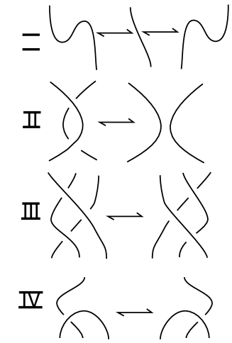
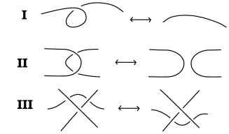
We shall call a link diagram arranged with respect to a direction in time a Morse diagram. Note that, generically, in a Morse diagram, a horizontal line in the plane intersects the diagram transversely in a finite collection of points. Special points or critical points consist in maxima and minima in the diagram, and the places where a crossing appears in the diagram. We can transform any link diagram into a Morse diagram by an isotopy of the plane and so all knots and links are represented by Morse diagrams. Before going further with Morse diagrams, we first recall that two diagrams, regarded as projections of knots or links in three-space, are equivalent by Reidemeister moves as shown in FigureΒ 5. This result, due to Reidemeister, Alexander and Briggs Reid , implies that the equivalence classes of diagrams generated by the Reidemeister moves classify the topological types of knots and links in three-dimensional space. In order to work with Morse diagrams, we use a refomulation of the Reidemeister Theorem that utilizes the move types shown in FigureΒ 6. The reformulation of the Reidemeister theorem RT1 ; RT2 ; TM ; Yetter states that two Morse link diagrams are equivalent via the Morse moves of FigureΒ 6 if and only if they are regularly isotopic. A good reference for the details of this theorem based on Reidemeister’s orginal approach can be found in the paper by David Yetter Yetter . Regular isotopy is the equivalence relation on diagrams generated by the second and third Reidemeister moves. Thus Morse diagrams and their moves give a complete formalism for the regular isotopy classification of standard knot and link diagrams. Regular isotopy invariance is often the most convenient method for studying knots and links. Invariants of regular isotopy can often be normalized to produce invariants of ambient isotopy (the equivalence relation generated by all three Reidemeister moves). In the following we shall detail how to use solutions of the Yang-Baxter equation to produce invariants of regular isotopy for Morse diagrams.

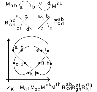
The strategy for this method to produce invariants is illustrated in FigureΒ 7 and FigureΒ 8. In the following we explain the use of Morse diagrams for producing link invariants. The original approach, due to Reshetikhin and Turaev RT1 ; RT2 , is formulated using the oriented tangle category. Our approach describes the analogous structure for unoriented diagrams and can be used as well for oriented diagrams. We divide the Morse diagram into parts that are the shape of a maxima, a minima or a crossing. We associate matrices Ma​bsuperscriptπ‘€π‘Žπ‘M^{ab} to minima, Ma​bsubscriptπ‘€π‘Žπ‘M_{ab} to maxima and Rc​da​bsubscriptsuperscriptπ‘…π‘Žπ‘π‘π‘‘R^{ab}_{cd} to crossings. Each choice of indices for any matrix gives a scalar quantity for the corresponding matrix entry. The diagram yields, as in FigureΒ 8, a product of these scalars with every index repeated twice. One then takes the summation of these products over all choices of indices. The resulting state summation ZKsubscript𝑍𝐾Z_{K} is the quantum link amplitude. In our physical metaphor, this is the quantum amplitude for the vacuum to vacuum process the involves the creation of particles via minima, the interaction of particles at the crossings and annihilations of particles at the maxima. The matrices must satisfy a collection of equations that correspond to the moves on Morse diagrams. We detail these equations and the correspondences below.
Refer to caption
Figure 5: Classical Reidemeister Moves
Refer to caption
Figure 6: Regular Isotopy With Respect to a Vertical Direction
Refer to caption
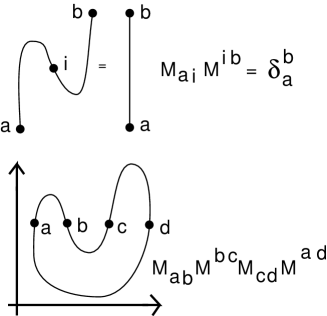
Figure 7: Jordan Curve Amplitude
Refer to caption
Figure 8: Amplitude for a Morse Diagram

All crossings in a link diagram are represented by transversal intersections. Any non-self-intersecting differentiable curve (for embedded curves and for transversely intersecting immersed curves) can be rigidly rotated until it is in general position with respect to the vertical. A curve without intersections is then seen to decompose into an interconnection of minima and maxima. We can evaluate an amplitude for any curve in this general position with respect to a vertical direction. Any simple closed curve in the plane is isotopic to a circle, by the Jordan Curve Theorem. If these are topological amplitudes, then the value for any simple closed curve should be equal to the amplitude of the circle. In order to find conditions for the creation and annihilation operators that ensure amplitudes that respect topological equivalence, isotopies of simple closed curves are generated by the cancellation of adjacent maxima and minima. Specifically, let e1,e2,…,ensubscript𝑒1subscript𝑒2…subscript𝑒𝑛{e_{1},e_{2},...,e_{n}} be a basis for V𝑉V. Let ea​b=eaβŠ—ebsubscriptπ‘’π‘Žπ‘tensor-productsubscriptπ‘’π‘Žsubscript𝑒𝑏e_{ab}=e_{a}\otimes e_{b} denote the elements of the tensor basis for VβŠ—Vtensor-product𝑉𝑉V\otimes V. Then, there are matrices Ma​bsubscriptπ‘€π‘Žπ‘M_{ab} and Ma​bsuperscriptπ‘€π‘Žπ‘M^{ab} such that

C​a​pπΆπ‘Žπ‘\textstyle{Cap}C​u​p𝐢𝑒𝑝\textstyle{Cup}R𝑅\textstyle{R}R¯¯𝑅\textstyle{\overline{R}}
Figure 9:
|c​u​pβŸ©β€‹(1)=βˆ‘Ma​b​ea​b,ket𝑐𝑒𝑝1superscriptπ‘€π‘Žπ‘subscriptπ‘’π‘Žπ‘\ket{cup}(1)=\sum{M^{ab}e_{ab}},

with the summation taken over all values of aπ‘Ža and b𝑏b from 111 to n𝑛n. Similarly, ⟨c​a​p|braπ‘π‘Žπ‘\bra{cap} is described by

⟨c​a​p|​(ea​b)=Ma​b.braπ‘π‘Žπ‘subscriptπ‘’π‘Žπ‘subscriptπ‘€π‘Žπ‘\bra{cap}(e_{ab})=M_{ab}.

Thus the amplitude for the circle is

⟨c​a​p|c​u​pβŸ©β€‹(1)=⟨c​a​p|β€‹βˆ‘Ma​b​ea​b=βˆ‘Ma​bβ€‹βŸ¨c​a​p|​(ea​b)=βˆ‘Ma​b​Ma​b.inner-productπ‘π‘Žπ‘π‘π‘’π‘1braπ‘π‘Žπ‘superscriptπ‘€π‘Žπ‘subscriptπ‘’π‘Žπ‘superscriptπ‘€π‘Žπ‘braπ‘π‘Žπ‘subscriptπ‘’π‘Žπ‘superscriptπ‘€π‘Žπ‘subscriptπ‘€π‘Žπ‘\braket{cap}{cup}(1)=\bra{cap}\sum{M^{ab}e_{ab}}=\sum{M^{ab}\bra{cap}(e_{ab})}=\sum{M^{ab}M_{ab}}.

In general, the value of the amplitude on a simple closed curve is obtained by translating it into an β€œabstract tensor expression” using Ma​bsuperscriptπ‘€π‘Žπ‘M^{ab} and Ma​bsubscriptπ‘€π‘Žπ‘M_{ab}, and then summing over the products for all cases of repeated indices. Note that here the value β€œ1” corresponds to the vacuum. For example in FigureΒ 7 we write down a more complex amplitude for a Jordan curve in the lower part of the figure. We also illustrate a topological relation on the matrices that will ensure that this evaluation is the same as the circle evaluation above. This topological relation is just that the matrices Ma​bsuperscriptπ‘€π‘Žπ‘M^{ab} and Mc​dsubscript𝑀𝑐𝑑M_{cd} are inverses in the sense that

βˆ‘iMa​i​Mi​b=Ξ΄ab,subscript𝑖subscriptπ‘€π‘Žπ‘–superscript𝑀𝑖𝑏subscriptsuperscriptπ›Ώπ‘π‘Ž\sum_{i}M_{ai}M^{ib}=\delta^{b}_{a},

where Ξ΄absubscriptsuperscriptπ›Ώπ‘π‘Ž\delta^{b}_{a} denotes the identity matrix. This equation is illustrated diagrammatically in FigureΒ 7.

One of our simplest choices is to take a 2Γ—2222\times 2 matrix M𝑀M such that M2=Isuperscript𝑀2𝐼M^{2}=I, where I𝐼I is the identity matrix. Then the entries of M𝑀M can be used for both the cup and the cap. The value for a loop is then equal to the sum of the squares of the entries of M𝑀M:

⟨c​a​p|c​u​p⟩=βˆ‘Ma​b​Ma​b=βˆ‘Ma​b​Ma​b=βˆ‘Ma​b2.inner-productπ‘π‘Žπ‘π‘π‘’π‘superscriptπ‘€π‘Žπ‘subscriptπ‘€π‘Žπ‘subscriptπ‘€π‘Žπ‘subscriptπ‘€π‘Žπ‘subscriptsuperscript𝑀2π‘Žπ‘\braket{cap}{cup}=\sum M^{ab}M_{ab}=\sum M_{ab}M_{ab}=\sum M^{2}_{ab}.

Any knot or link can be represented by a picture that is configured with respect to a vertical direction in the plane. The picture decomposes into minima (creations), maxima (annihilations), and crossings of the two types shown in FigureΒ 8 and FigureΒ 9. Here the knots and links are unoriented. Any knot or link can be written as a composition of these fragments, and consequently a choice of such mappings determines an amplitude for knots and links. In order for such an amplitude to be topological (i.e. an invariant of regular isotopy of the equivalence relation generated by the second and third classical Reidemeister moves) we want it to be invariant under a list of local moves as shown in FigureΒ 10, FigureΒ 11, FigureΒ 12, FigureΒ 13.

We now give an explanation of the algebraic and topological equations shown in these figures. FigureΒ 10 is the cancellation of maxima and minima. FigureΒ 11 corresponds to the second Reidemeister move. FigureΒ 12 is the Yang-Baxter equation. FigureΒ 13 demonstrates that a line can move across a minimum (similar equations can be formulated for a line moving across a maximum). In each figure we have given the corresponding equation for the cup, cap and crossing matrix elements. If these equations are taken purely abstractly then they indicate a necessary and sufficient condition for a state sum of this type to be an invariant of regular isotopy. In order to produce an invariant, it is sufficient that the matrices satisfy these conditions. Such an invariant is not necessarily a complete invariant of regular isotopy, and to this date no one has produced such a complete invariant other than the formalism itself.

abi=baπ‘Žπ‘π‘–π‘π‘Ž\lx@xy@svg{\hbox{\raise 0.0pt\hbox{\kern 28.25029pt\hbox{{}{}{}{}{}\ignorespaces\hbox{\hbox{\kern 0.0pt\raise 0.0pt\hbox{{}{}{{}{}}{{}{}{}{}\lx@xy@spline@}{}}}}\ignorespaces{}{}{}{}{{}{{}{{}{{}{{}{{}{{}}{}{{}}{}{{}}{}{{}}{}{{}{{}}{}{{}}}}}}}}}{\hbox{\kern-0.04529pt\raise 2.48631pt\hbox{\hbox{\kern 0.0pt\raise 0.0pt\hbox{\lower-4.99657pt\hbox{\line@@}}}}}}\ignorespaces{}{}{}{}{{}}{\hbox{\kern-17.07156pt\raise 0.0pt\hbox{\hbox{\kern 0.0pt\raise 0.0pt\hbox{\hbox{\line@@}}}}}}\ignorespaces\hbox{\hbox{\kern 0.0pt\raise 0.0pt\hbox{{}{}{{}{}}{{}{}{}{}\lx@xy@spline@}{}}}}\ignorespaces{}{}{}{}{{}{{}{{}{{}{{}{{}{{}}{}{{}}{}{{}}{}{{}}{}{{}{{}}{}{{}}}}}}}}}{\hbox{\kern 17.02634pt\raise-2.48631pt\hbox{\hbox{\kern 0.0pt\raise 0.0pt\hbox{\lower 4.99657pt\hbox{\line@@}}}}}}\ignorespaces\ignorespaces{\hbox{\lx@xy@droprule}}\ignorespaces\ignorespaces{\hbox{\lx@xy@droprule}}{\hbox{\kern-28.25029pt\raise-14.2263pt\hbox{\hbox{\kern 0.0pt\raise-2.15277pt\hbox{$\textstyle{a}$}}}}}{\hbox{\kern 23.46152pt\raise 14.2263pt\hbox{\hbox{\kern 0.0pt\raise-3.47223pt\hbox{$\textstyle{b}$}}}}}{\hbox{\kern 3.96796pt\raise 0.0pt\hbox{\hbox{\kern 0.0pt\raise-3.29762pt\hbox{$\textstyle{i}$}}}}}}}}}\qquad=\qquad\lx@xy@svg{\hbox{\raise 0.0pt\hbox{\kern 7.83635pt\hbox{{}{}\ignorespaces\ignorespaces{\hbox{\lx@xy@droprule}}{\hbox{\kern-7.83635pt\raise 28.4526pt\hbox{\hbox{\kern 0.0pt\raise-3.47223pt\hbox{$\textstyle{b}$}}}}}{\hbox{\kern 3.04758pt\raise-28.4526pt\hbox{\hbox{\kern 0.0pt\raise-2.15277pt\hbox{$\textstyle{a}$}}}}}}}}}
Figure 10: Ma​i​Mi​b=Ξ΄absubscriptπ‘€π‘Žπ‘–superscript𝑀𝑖𝑏subscriptsuperscriptπ›Ώπ‘π‘ŽM_{ai}M^{ib}=\delta^{b}_{a}
Β Β abijcd=abcdΒ Β π‘Žπ‘π‘–π‘—π‘π‘‘π‘Žπ‘π‘π‘‘\lx@xy@svg{\hbox{\raise 0.0pt\hbox{\kern 21.63939pt\hbox{\ignorespaces\ignorespaces\ignorespaces\ignorespaces\ignorespaces\ignorespaces\ignorespaces\ignorespaces\ignorespaces\ignorespaces\ignorespaces\ignorespaces\ignorespaces\ignorespaces\ignorespaces\ignorespaces\ignorespaces\ignorespaces\ignorespaces\ignorespaces\ignorespaces\ignorespaces\ignorespaces\ignorespaces\ignorespaces\ignorespaces{}{}{}{}{}{{}}{}\ignorespaces\ignorespaces\hbox{\hbox{\kern 0.0pt\raise 0.0pt\hbox{{}{}{}\ignorespaces\ignorespaces{{}{}{}{}\ignorespaces{}}{{}{}{}\ignorespaces{}}{{}{}{}}{}}}}\ignorespaces{}\ignorespaces{}{{}{}}{{}}{}{{}}{}\ignorespaces\ignorespaces\hbox{\hbox{\kern 0.0pt\raise 0.0pt\hbox{{}{}{}{}\ignorespaces\ignorespaces{{}{}{}{}\ignorespaces{}\lx@xy@spline@}{{}{}{}\ignorespaces{}\lx@xy@spline@}{{}{}{}\lx@xy@spline@}{}}}}\ignorespaces{}\ignorespaces\hbox{\hbox{\kern 0.0pt\raise 0.0pt\hbox{{}{}{}\ignorespaces\ignorespaces{{}{}{}{}\ignorespaces{}}{{}{}{}\ignorespaces{}}{{}{}{}}{}}}}\ignorespaces{}\ignorespaces\ignorespaces\ignorespaces\ignorespaces\ignorespaces\ignorespaces\ignorespaces\ignorespaces\ignorespaces\ignorespaces\ignorespaces\ignorespaces\ignorespaces\ignorespaces\ignorespaces\ignorespaces\ignorespaces\ignorespaces\ignorespaces{}{}{}{}{}{{}}{}\ignorespaces\ignorespaces\hbox{\hbox{\kern 0.0pt\raise 0.0pt\hbox{{}{}{}\ignorespaces\ignorespaces{{}{}{}{}\ignorespaces{}}{{}{}{}\ignorespaces{}}{{}{}{}}{}}}}\ignorespaces{}\ignorespaces{}{}{{}}{}{}{{}{{}}}{\hbox{\kern-2.5pt\raise-7.11316pt\hbox{\hbox{\kern 0.0pt\raise 0.0pt\hbox{$\scriptstyle{\hbox to5.0pt{\hfill\vrule height=2.5pt,depth=2.5pt,width=0.0pt}}$}}}}}\ignorespaces\ignorespaces\hbox{\hbox{\kern 0.0pt\raise 0.0pt\hbox{{}{}{}{{}{}{{}}{}{}{{{}}{{{}}}{{}}{{{}}{{{}}{{{}}{{{}}{{{}}{{{}}{{{}}{{{}}{{{}}{{{}}{{{}}{{{}}{{{}}{}{{{}}}{{}}}{{}}}{{}}}{{}}}{{}}}{{}}}{{}}}{{}}}{{}}}{{}}}{{}}}{{}}}{{}}}{{}}{{{}}{{{}}{{{}}{{{}}{{{}}}{{}}{{{}}}{{}}{{{}}{{{}}{{{}}{{{}}}{{}}{{{}}{{{}}}{{}}{}}}}}}}}}}}\ignorespaces\ignorespaces{{}{}{}{}\ignorespaces{}\lx@xy@spline@}{{}{}{}\ignorespaces{}\lx@xy@spline@}{{}{}{}}{}}}}\ignorespaces{}\ignorespaces{}{{}{}}{{}}{}{{}}{}\ignorespaces\ignorespaces\hbox{\hbox{\kern 0.0pt\raise 0.0pt\hbox{{}{{}{}{{}}{}{}{{{}}{{{}}{}}{{{}}}{{}}{{{}}{{{}}{{{}}{{{}}{{{}}}{{}}{{{}}}{{}}{{{}}{{{}}{{{}}{{{}}}{{}}{{{}}{{{}}}{{}}}}}}}}}}}}{}{}\ignorespaces\ignorespaces{{}{}{}{}\ignorespaces{}}{{}{}{}\ignorespaces{}\lx@xy@spline@}{{}{}{}\lx@xy@spline@}{}}}}\ignorespaces{}\ignorespaces\hbox{\hbox{\kern 0.0pt\raise 0.0pt\hbox{{}{}{}\ignorespaces\ignorespaces{{}{}{}{}\ignorespaces{}}{{}{}{}\ignorespaces{}}{{}{}{}}{}}}}\ignorespaces{}\ignorespaces\ignorespaces\ignorespaces\ignorespaces\ignorespaces\ignorespaces\ignorespaces\ignorespaces\ignorespaces\ignorespaces\ignorespaces\ignorespaces\ignorespaces\ignorespaces\ignorespaces\ignorespaces\ignorespaces\ignorespaces\ignorespaces\ignorespaces\ignorespaces\ignorespaces\ignorespaces\ignorespaces\ignorespaces\ignorespaces\ignorespaces\ignorespaces\ignorespaces\ignorespaces{}{}{}{}{}{{}}{}\ignorespaces\ignorespaces\hbox{\hbox{\kern 0.0pt\raise 0.0pt\hbox{{}{}{}\ignorespaces\ignorespaces{{}{}{}{}\ignorespaces{}}{{}{}{}\ignorespaces{}}{{}{}{}}{}}}}\ignorespaces{}\ignorespaces{}{{}{}}{{}}{}{{}}{}\ignorespaces\ignorespaces\hbox{\hbox{\kern 0.0pt\raise 0.0pt\hbox{{}{}{}{}\ignorespaces\ignorespaces{{}{}{}{}\ignorespaces{}\lx@xy@spline@}{{}{}{}\ignorespaces{}\lx@xy@spline@}{{}{}{}\lx@xy@spline@}{}}}}\ignorespaces{}\ignorespaces\hbox{\hbox{\kern 0.0pt\raise 0.0pt\hbox{{}{}{}\ignorespaces\ignorespaces{{}{}{}{}\ignorespaces{}}{{}{}{}\ignorespaces{}}{{}{}{}}{}}}}\ignorespaces{}\ignorespaces\ignorespaces\ignorespaces\ignorespaces\ignorespaces\ignorespaces\ignorespaces\ignorespaces\ignorespaces\ignorespaces\ignorespaces\ignorespaces\ignorespaces\ignorespaces\ignorespaces\ignorespaces\ignorespaces\ignorespaces\ignorespaces{}{}{}{}{}{{}}{}\ignorespaces\ignorespaces\hbox{\hbox{\kern 0.0pt\raise 0.0pt\hbox{{}{}{}\ignorespaces\ignorespaces{{}{}{}{}\ignorespaces{}}{{}{}{}\ignorespaces{}}{{}{}{}}{}}}}\ignorespaces{}\ignorespaces{}{}{{}}{}{}{{}{{}}}{\hbox{\kern-2.5pt\raise-42.67891pt\hbox{\hbox{\kern 0.0pt\raise 0.0pt\hbox{$\scriptstyle{\hbox to5.0pt{\hfill\vrule height=2.5pt,depth=2.5pt,width=0.0pt}}$}}}}}\ignorespaces\ignorespaces\hbox{\hbox{\kern 0.0pt\raise 0.0pt\hbox{{}{}{}{{}{}{{}}{}{}{{{}}{{{}}}{{}}{{{}}{{{}}{{{}}{{{}}{{{}}{{{}}{{{}}{{{}}{{{}}{{{}}{{{}}{{{}}{{{}}{}{{{}}}{{}}}{{}}}{{}}}{{}}}{{}}}{{}}}{{}}}{{}}}{{}}}{{}}}{{}}}{{}}}{{}}}{{}}{{{}}{{{}}{{{}}{{{}}{{{}}}{{}}{{{}}}{{}}{{{}}{{{}}{{{}}{{{}}}{{}}{{{}}{{{}}}{{}}{}}}}}}}}}}}\ignorespaces\ignorespaces{{}{}{}{}\ignorespaces{}\lx@xy@spline@}{{}{}{}\ignorespaces{}\lx@xy@spline@}{{}{}{}}{}}}}\ignorespaces{}\ignorespaces{}{{}{}}{{}}{}{{}}{}\ignorespaces\ignorespaces\hbox{\hbox{\kern 0.0pt\raise 0.0pt\hbox{{}{{}{}{{}}{}{}{{{}}{{{}}{}}{{{}}}{{}}{{{}}{{{}}{{{}}{{{}}{{{}}}{{}}{{{}}}{{}}{{{}}{{{}}{{{}}{{{}}}{{}}{{{}}{{{}}}{{}}}}}}}}}}}}{}{}\ignorespaces\ignorespaces{{}{}{}{}\ignorespaces{}}{{}{}{}\ignorespaces{}\lx@xy@spline@}{{}{}{}\lx@xy@spline@}{}}}}\ignorespaces{}\ignorespaces\hbox{\hbox{\kern 0.0pt\raise 0.0pt\hbox{{}{}{}\ignorespaces\ignorespaces{{}{}{}{}\ignorespaces{}}{{}{}{}\ignorespaces{}}{{}{}{}}{}}}}\ignorespaces{}\ignorespaces\ignorespaces\ignorespaces\ignorespaces{\hbox{\kern-16.86925pt\raise 19.91682pt\hbox{\hbox{\kern 0.0pt\raise-2.15277pt\hbox{$\textstyle{a}$}}}}}{\hbox{\kern 12.08047pt\raise 19.91682pt\hbox{\hbox{\kern 0.0pt\raise-3.47223pt\hbox{$\textstyle{b}$}}}}}{\hbox{\kern-21.63939pt\raise-28.4526pt\hbox{\hbox{\kern 0.0pt\raise-3.29762pt\hbox{$\textstyle{i}$}}}}}{\hbox{\kern 17.57158pt\raise-28.4526pt\hbox{\hbox{\kern 0.0pt\raise-2.32541pt\hbox{$\textstyle{j}$}}}}}{\hbox{\kern-16.39008pt\raise-62.59573pt\hbox{\hbox{\kern 0.0pt\raise-2.15277pt\hbox{$\textstyle{c}$}}}}}{\hbox{\kern 11.62387pt\raise-62.59573pt\hbox{\hbox{\kern 0.0pt\raise-3.47223pt\hbox{$\textstyle{d}$}}}}}}}}}\qquad=\qquad\lx@xy@svg{\hbox{\raise 0.0pt\hbox{\kern 16.86925pt\hbox{{}{}\ignorespaces\ignorespaces{\hbox{\lx@xy@droprule}}{}{}\ignorespaces\ignorespaces{\hbox{\lx@xy@droprule}}{\hbox{\kern-16.86925pt\raise 19.91682pt\hbox{\hbox{\kern 0.0pt\raise-2.15277pt\hbox{$\textstyle{a}$}}}}}{\hbox{\kern 12.08047pt\raise 19.91682pt\hbox{\hbox{\kern 0.0pt\raise-3.47223pt\hbox{$\textstyle{b}$}}}}}{\hbox{\kern-16.39008pt\raise-62.59573pt\hbox{\hbox{\kern 0.0pt\raise-2.15277pt\hbox{$\textstyle{c}$}}}}}{\hbox{\kern 11.62387pt\raise-62.59573pt\hbox{\hbox{\kern 0.0pt\raise-3.47223pt\hbox{$\textstyle{d}$}}}}}}}}}
Figure 11: Ri​ja​b¯​Rc​di​j=Ξ΄ca​δdbΒ―subscriptsuperscriptπ‘…π‘Žπ‘π‘–π‘—subscriptsuperscript𝑅𝑖𝑗𝑐𝑑subscriptsuperscriptπ›Ώπ‘Žπ‘subscriptsuperscript𝛿𝑏𝑑\overline{R^{ab}_{ij}}R^{ij}_{cd}=\delta^{a}_{c}\delta^{b}_{d}
Β Β Β abcefgijk=Β Β Β abcefgjkiΒ Β Β π‘Žπ‘π‘π‘’π‘“π‘”π‘–π‘—π‘˜Β Β Β π‘Žπ‘π‘π‘’π‘“π‘”π‘—π‘˜π‘–\lx@xy@svg{\hbox{\raise 0.0pt\hbox{\kern 21.63939pt\hbox{\ignorespaces\ignorespaces\ignorespaces\ignorespaces\ignorespaces\ignorespaces\ignorespaces\ignorespaces\ignorespaces\ignorespaces\ignorespaces\ignorespaces\ignorespaces\ignorespaces\ignorespaces\ignorespaces\ignorespaces\ignorespaces\ignorespaces\ignorespaces\ignorespaces\ignorespaces\ignorespaces\ignorespaces\ignorespaces\ignorespaces{}{}{}{}{}{{}}{}\ignorespaces\ignorespaces\hbox{\hbox{\kern 0.0pt\raise 0.0pt\hbox{{}{}{}\ignorespaces\ignorespaces{{}{}{}{}\ignorespaces{}}{{}{}{}\ignorespaces{}}{{}{}{}}{}}}}\ignorespaces{}\ignorespaces{}{{}{}}{{}}{}{{}}{}\ignorespaces\ignorespaces\hbox{\hbox{\kern 0.0pt\raise 0.0pt\hbox{{}{}{}{}\ignorespaces\ignorespaces{{}{}{}{}\ignorespaces{}\lx@xy@spline@}{{}{}{}\ignorespaces{}\lx@xy@spline@}{{}{}{}\lx@xy@spline@}{}}}}\ignorespaces{}\ignorespaces\hbox{\hbox{\kern 0.0pt\raise 0.0pt\hbox{{}{}{}\ignorespaces\ignorespaces{{}{}{}{}\ignorespaces{}}{{}{}{}\ignorespaces{}}{{}{}{}}{}}}}\ignorespaces{}\ignorespaces\ignorespaces\ignorespaces\ignorespaces\ignorespaces\ignorespaces\ignorespaces\ignorespaces\ignorespaces\ignorespaces\ignorespaces\ignorespaces\ignorespaces\ignorespaces\ignorespaces\ignorespaces\ignorespaces\ignorespaces\ignorespaces{}{}{}{}{}{{}}{}\ignorespaces\ignorespaces\hbox{\hbox{\kern 0.0pt\raise 0.0pt\hbox{{}{}{}\ignorespaces\ignorespaces{{}{}{}{}\ignorespaces{}}{{}{}{}\ignorespaces{}}{{}{}{}}{}}}}\ignorespaces{}\ignorespaces{}{}{{}}{}{}{{}{{}}}{\hbox{\kern-2.5pt\raise 14.2263pt\hbox{\hbox{\kern 0.0pt\raise 0.0pt\hbox{$\scriptstyle{\hbox to5.0pt{\hfill\vrule height=2.5pt,depth=2.5pt,width=0.0pt}}$}}}}}\ignorespaces\ignorespaces\hbox{\hbox{\kern 0.0pt\raise 0.0pt\hbox{{}{}{}{{}{}{{}}{}{}{{{}}{{{}}}{{}}{{{}}{{{}}{{{}}{{{}}{{{}}{{{}}{{{}}{{{}}{{{}}{{{}}{{{}}{{{}}{{{}}{}{{{}}}{{}}}{{}}}{{}}}{{}}}{{}}}{{}}}{{}}}{{}}}{{}}}{{}}}{{}}}{{}}}{{}}}{{}}{{{}}{{{}}{{{}}{{{}}{{{}}}{{}}{{{}}}{{}}{{{}}{{{}}{{{}}{{{}}}{{}}{{{}}{{{}}}{{}}{}}}}}}}}}}}\ignorespaces\ignorespaces{{}{}{}{}\ignorespaces{}\lx@xy@spline@}{{}{}{}\ignorespaces{}\lx@xy@spline@}{{}{}{}}{}}}}\ignorespaces{}\ignorespaces{}{{}{}}{{}}{}{{}}{}\ignorespaces\ignorespaces\hbox{\hbox{\kern 0.0pt\raise 0.0pt\hbox{{}{{}{}{{}}{}{}{{{}}{{{}}{}}{{{}}}{{}}{{{}}{{{}}{{{}}{{{}}{{{}}}{{}}{{{}}}{{}}{{{}}{{{}}{{{}}{{{}}}{{}}{{{}}{{{}}}{{}}}}}}}}}}}}{}{}\ignorespaces\ignorespaces{{}{}{}{}\ignorespaces{}}{{}{}{}\ignorespaces{}\lx@xy@spline@}{{}{}{}\lx@xy@spline@}{}}}}\ignorespaces{}\ignorespaces\hbox{\hbox{\kern 0.0pt\raise 0.0pt\hbox{{}{}{}\ignorespaces\ignorespaces{{}{}{}{}\ignorespaces{}}{{}{}{}\ignorespaces{}}{{}{}{}}{}}}}\ignorespaces{}\ignorespaces\ignorespaces\ignorespaces\ignorespaces{}{}\ignorespaces\ignorespaces{\hbox{\lx@xy@droprule}}\ignorespaces\ignorespaces\ignorespaces\ignorespaces\ignorespaces\ignorespaces\ignorespaces\ignorespaces\ignorespaces\ignorespaces\ignorespaces\ignorespaces\ignorespaces\ignorespaces\ignorespaces\ignorespaces\ignorespaces\ignorespaces\ignorespaces\ignorespaces\ignorespaces\ignorespaces\ignorespaces\ignorespaces\ignorespaces\ignorespaces{}{}{}{}{}{{}}{}\ignorespaces\ignorespaces\hbox{\hbox{\kern 0.0pt\raise 0.0pt\hbox{{}{}{}\ignorespaces\ignorespaces{{}{}{}{}\ignorespaces{}}{{}{}{}\ignorespaces{}}{{}{}{}}{}}}}\ignorespaces{}\ignorespaces{}{{}{}}{{}}{}{{}}{}\ignorespaces\ignorespaces\hbox{\hbox{\kern 0.0pt\raise 0.0pt\hbox{{}{}{}{}\ignorespaces\ignorespaces{{}{}{}{}\ignorespaces{}\lx@xy@spline@}{{}{}{}\ignorespaces{}\lx@xy@spline@}{{}{}{}\lx@xy@spline@}{}}}}\ignorespaces{}\ignorespaces\hbox{\hbox{\kern 0.0pt\raise 0.0pt\hbox{{}{}{}\ignorespaces\ignorespaces{{}{}{}{}\ignorespaces{}}{{}{}{}\ignorespaces{}}{{}{}{}}{}}}}\ignorespaces{}\ignorespaces\ignorespaces\ignorespaces\ignorespaces\ignorespaces\ignorespaces\ignorespaces\ignorespaces\ignorespaces\ignorespaces\ignorespaces\ignorespaces\ignorespaces\ignorespaces\ignorespaces\ignorespaces\ignorespaces\ignorespaces\ignorespaces{}{}{}{}{}{{}}{}\ignorespaces\ignorespaces\hbox{\hbox{\kern 0.0pt\raise 0.0pt\hbox{{}{}{}\ignorespaces\ignorespaces{{}{}{}{}\ignorespaces{}}{{}{}{}\ignorespaces{}}{{}{}{}}{}}}}\ignorespaces{}\ignorespaces{}{}{{}}{}{}{{}{{}}}{\hbox{\kern 25.95262pt\raise-14.2263pt\hbox{\hbox{\kern 0.0pt\raise 0.0pt\hbox{$\scriptstyle{\hbox to5.0pt{\hfill\vrule height=2.5pt,depth=2.5pt,width=0.0pt}}$}}}}}\ignorespaces\ignorespaces\hbox{\hbox{\kern 0.0pt\raise 0.0pt\hbox{{}{}{}{{}{}{{}}{}{}{{{}}{{{}}}{{}}{{{}}{{{}}{{{}}{{{}}{{{}}{{{}}{{{}}{{{}}{{{}}{{{}}{{{}}{{{}}{{{}}{}{{{}}}{{}}}{{}}}{{}}}{{}}}{{}}}{{}}}{{}}}{{}}}{{}}}{{}}}{{}}}{{}}}{{}}}{{}}{{{}}{{{}}{{{}}{{{}}{{{}}}{{}}{{{}}}{{}}{{{}}{{{}}{{{}}{{{}}}{{}}{{{}}{{{}}}{{}}{}}}}}}}}}}}\ignorespaces\ignorespaces{{}{}{}{}\ignorespaces{}\lx@xy@spline@}{{}{}{}\ignorespaces{}\lx@xy@spline@}{{}{}{}}{}}}}\ignorespaces{}\ignorespaces{}{{}{}}{{}}{}{{}}{}\ignorespaces\ignorespaces\hbox{\hbox{\kern 0.0pt\raise 0.0pt\hbox{{}{{}{}{{}}{}{}{{{}}{{{}}{}}{{{}}}{{}}{{{}}{{{}}{{{}}{{{}}{{{}}}{{}}{{{}}}{{}}{{{}}{{{}}{{{}}{{{}}}{{}}{{{}}{{{}}}{{}}}}}}}}}}}}{}{}\ignorespaces\ignorespaces{{}{}{}{}\ignorespaces{}}{{}{}{}\ignorespaces{}\lx@xy@spline@}{{}{}{}\lx@xy@spline@}{}}}}\ignorespaces{}\ignorespaces\hbox{\hbox{\kern 0.0pt\raise 0.0pt\hbox{{}{}{}\ignorespaces\ignorespaces{{}{}{}{}\ignorespaces{}}{{}{}{}\ignorespaces{}}{{}{}{}}{}}}}\ignorespaces{}\ignorespaces\ignorespaces\ignorespaces\ignorespaces{}{}\ignorespaces\ignorespaces{\hbox{\lx@xy@droprule}}\ignorespaces\ignorespaces\ignorespaces\ignorespaces\ignorespaces\ignorespaces\ignorespaces\ignorespaces\ignorespaces\ignorespaces\ignorespaces\ignorespaces\ignorespaces\ignorespaces\ignorespaces\ignorespaces\ignorespaces\ignorespaces\ignorespaces\ignorespaces\ignorespaces\ignorespaces\ignorespaces\ignorespaces\ignorespaces\ignorespaces{}{}{}{}{}{{}}{}\ignorespaces\ignorespaces\hbox{\hbox{\kern 0.0pt\raise 0.0pt\hbox{{}{}{}\ignorespaces\ignorespaces{{}{}{}{}\ignorespaces{}}{{}{}{}\ignorespaces{}}{{}{}{}}{}}}}\ignorespaces{}\ignorespaces{}{{}{}}{{}}{}{{}}{}\ignorespaces\ignorespaces\hbox{\hbox{\kern 0.0pt\raise 0.0pt\hbox{{}{}{}{}\ignorespaces\ignorespaces{{}{}{}{}\ignorespaces{}\lx@xy@spline@}{{}{}{}\ignorespaces{}\lx@xy@spline@}{{}{}{}\lx@xy@spline@}{}}}}\ignorespaces{}\ignorespaces\hbox{\hbox{\kern 0.0pt\raise 0.0pt\hbox{{}{}{}\ignorespaces\ignorespaces{{}{}{}{}\ignorespaces{}}{{}{}{}\ignorespaces{}}{{}{}{}}{}}}}\ignorespaces{}\ignorespaces\ignorespaces\ignorespaces\ignorespaces\ignorespaces\ignorespaces\ignorespaces\ignorespaces\ignorespaces\ignorespaces\ignorespaces\ignorespaces\ignorespaces\ignorespaces\ignorespaces\ignorespaces\ignorespaces\ignorespaces\ignorespaces{}{}{}{}{}{{}}{}\ignorespaces\ignorespaces\hbox{\hbox{\kern 0.0pt\raise 0.0pt\hbox{{}{}{}\ignorespaces\ignorespaces{{}{}{}{}\ignorespaces{}}{{}{}{}\ignorespaces{}}{{}{}{}}{}}}}\ignorespaces{}\ignorespaces{}{}{{}}{}{}{{}{{}}}{\hbox{\kern-2.5pt\raise-42.67891pt\hbox{\hbox{\kern 0.0pt\raise 0.0pt\hbox{$\scriptstyle{\hbox to5.0pt{\hfill\vrule height=2.5pt,depth=2.5pt,width=0.0pt}}$}}}}}\ignorespaces\ignorespaces\hbox{\hbox{\kern 0.0pt\raise 0.0pt\hbox{{}{}{}{{}{}{{}}{}{}{{{}}{{{}}}{{}}{{{}}{{{}}{{{}}{{{}}{{{}}{{{}}{{{}}{{{}}{{{}}{{{}}{{{}}{{{}}{{{}}{}{{{}}}{{}}}{{}}}{{}}}{{}}}{{}}}{{}}}{{}}}{{}}}{{}}}{{}}}{{}}}{{}}}{{}}}{{}}{{{}}{{{}}{{{}}{{{}}{{{}}}{{}}{{{}}}{{}}{{{}}{{{}}{{{}}{{{}}}{{}}{{{}}{{{}}}{{}}{}}}}}}}}}}}\ignorespaces\ignorespaces{{}{}{}{}\ignorespaces{}\lx@xy@spline@}{{}{}{}\ignorespaces{}\lx@xy@spline@}{{}{}{}}{}}}}\ignorespaces{}\ignorespaces{}{{}{}}{{}}{}{{}}{}\ignorespaces\ignorespaces\hbox{\hbox{\kern 0.0pt\raise 0.0pt\hbox{{}{{}{}{{}}{}{}{{{}}{{{}}{}}{{{}}}{{}}{{{}}{{{}}{{{}}{{{}}{{{}}}{{}}{{{}}}{{}}{{{}}{{{}}{{{}}{{{}}}{{}}{{{}}{{{}}}{{}}}}}}}}}}}}{}{}\ignorespaces\ignorespaces{{}{}{}{}\ignorespaces{}}{{}{}{}\ignorespaces{}\lx@xy@spline@}{{}{}{}\lx@xy@spline@}{}}}}\ignorespaces{}\ignorespaces\hbox{\hbox{\kern 0.0pt\raise 0.0pt\hbox{{}{}{}\ignorespaces\ignorespaces{{}{}{}{}\ignorespaces{}}{{}{}{}\ignorespaces{}}{{}{}{}}{}}}}\ignorespaces{}\ignorespaces\ignorespaces\ignorespaces\ignorespaces{}{}\ignorespaces\ignorespaces{\hbox{\lx@xy@droprule}}{\hbox{\kern-16.86925pt\raise 34.14313pt\hbox{\hbox{\kern 0.0pt\raise-2.15277pt\hbox{$\textstyle{a}$}}}}}{\hbox{\kern 12.08047pt\raise 34.14313pt\hbox{\hbox{\kern 0.0pt\raise-3.47223pt\hbox{$\textstyle{b}$}}}}}{\hbox{\kern 40.51514pt\raise 34.14313pt\hbox{\hbox{\kern 0.0pt\raise-2.15277pt\hbox{$\textstyle{c}$}}}}}{\hbox{\kern-16.55443pt\raise-62.59573pt\hbox{\hbox{\kern 0.0pt\raise-2.15277pt\hbox{$\textstyle{e}$}}}}}{\hbox{\kern 11.24017pt\raise-62.59573pt\hbox{\hbox{\kern 0.0pt\raise-2.5pt\hbox{$\textstyle{f}$}}}}}{\hbox{\kern 40.11469pt\raise-62.59573pt\hbox{\hbox{\kern 0.0pt\raise-1.18056pt\hbox{$\textstyle{g}$}}}}}{\hbox{\kern-21.63939pt\raise-14.2263pt\hbox{\hbox{\kern 0.0pt\raise-3.29762pt\hbox{$\textstyle{i}$}}}}}{\hbox{\kern 20.41684pt\raise 5.69052pt\hbox{\hbox{\kern 0.0pt\raise-2.32541pt\hbox{$\textstyle{j}$}}}}}{\hbox{\kern 20.00166pt\raise-25.60735pt\hbox{\hbox{\kern 0.0pt\raise-3.47223pt\hbox{$\textstyle{k}$}}}}}}}}}\qquad=\qquad\lx@xy@svg{\hbox{\raise 0.0pt\hbox{\kern 16.86925pt\hbox{\ignorespaces\ignorespaces\ignorespaces\ignorespaces\ignorespaces\ignorespaces\ignorespaces\ignorespaces\ignorespaces\ignorespaces\ignorespaces\ignorespaces\ignorespaces\ignorespaces\ignorespaces\ignorespaces\ignorespaces\ignorespaces\ignorespaces\ignorespaces\ignorespaces\ignorespaces\ignorespaces\ignorespaces\ignorespaces\ignorespaces{}{}{}{}{}{{}}{}\ignorespaces\ignorespaces\hbox{\hbox{\kern 0.0pt\raise 0.0pt\hbox{{}{}{}\ignorespaces\ignorespaces{{}{}{}{}\ignorespaces{}}{{}{}{}\ignorespaces{}}{{}{}{}}{}}}}\ignorespaces{}\ignorespaces{}{{}{}}{{}}{}{{}}{}\ignorespaces\ignorespaces\hbox{\hbox{\kern 0.0pt\raise 0.0pt\hbox{{}{}{}{}\ignorespaces\ignorespaces{{}{}{}{}\ignorespaces{}\lx@xy@spline@}{{}{}{}\ignorespaces{}\lx@xy@spline@}{{}{}{}\lx@xy@spline@}{}}}}\ignorespaces{}\ignorespaces\hbox{\hbox{\kern 0.0pt\raise 0.0pt\hbox{{}{}{}\ignorespaces\ignorespaces{{}{}{}{}\ignorespaces{}}{{}{}{}\ignorespaces{}}{{}{}{}}{}}}}\ignorespaces{}\ignorespaces\ignorespaces\ignorespaces\ignorespaces\ignorespaces\ignorespaces\ignorespaces\ignorespaces\ignorespaces\ignorespaces\ignorespaces\ignorespaces\ignorespaces\ignorespaces\ignorespaces\ignorespaces\ignorespaces\ignorespaces\ignorespaces{}{}{}{}{}{{}}{}\ignorespaces\ignorespaces\hbox{\hbox{\kern 0.0pt\raise 0.0pt\hbox{{}{}{}\ignorespaces\ignorespaces{{}{}{}{}\ignorespaces{}}{{}{}{}\ignorespaces{}}{{}{}{}}{}}}}\ignorespaces{}\ignorespaces{}{}{{}}{}{}{{}{{}}}{\hbox{\kern 25.95262pt\raise 14.2263pt\hbox{\hbox{\kern 0.0pt\raise 0.0pt\hbox{$\scriptstyle{\hbox to5.0pt{\hfill\vrule height=2.5pt,depth=2.5pt,width=0.0pt}}$}}}}}\ignorespaces\ignorespaces\hbox{\hbox{\kern 0.0pt\raise 0.0pt\hbox{{}{}{}{{}{}{{}}{}{}{{{}}{{{}}}{{}}{{{}}{{{}}{{{}}{{{}}{{{}}{{{}}{{{}}{{{}}{{{}}{{{}}{{{}}{{{}}{{{}}{}{{{}}}{{}}}{{}}}{{}}}{{}}}{{}}}{{}}}{{}}}{{}}}{{}}}{{}}}{{}}}{{}}}{{}}}{{}}{{{}}{{{}}{{{}}{{{}}{{{}}}{{}}{{{}}}{{}}{{{}}{{{}}{{{}}{{{}}}{{}}{{{}}{{{}}}{{}}{}}}}}}}}}}}\ignorespaces\ignorespaces{{}{}{}{}\ignorespaces{}\lx@xy@spline@}{{}{}{}\ignorespaces{}\lx@xy@spline@}{{}{}{}}{}}}}\ignorespaces{}\ignorespaces{}{{}{}}{{}}{}{{}}{}\ignorespaces\ignorespaces\hbox{\hbox{\kern 0.0pt\raise 0.0pt\hbox{{}{{}{}{{}}{}{}{{{}}{{{}}{}}{{{}}}{{}}{{{}}{{{}}{{{}}{{{}}{{{}}}{{}}{{{}}}{{}}{{{}}{{{}}{{{}}{{{}}}{{}}{{{}}{{{}}}{{}}}}}}}}}}}}{}{}\ignorespaces\ignorespaces{{}{}{}{}\ignorespaces{}}{{}{}{}\ignorespaces{}\lx@xy@spline@}{{}{}{}\lx@xy@spline@}{}}}}\ignorespaces{}\ignorespaces\hbox{\hbox{\kern 0.0pt\raise 0.0pt\hbox{{}{}{}\ignorespaces\ignorespaces{{}{}{}{}\ignorespaces{}}{{}{}{}\ignorespaces{}}{{}{}{}}{}}}}\ignorespaces{}\ignorespaces\ignorespaces\ignorespaces\ignorespaces{}{}\ignorespaces\ignorespaces{\hbox{\lx@xy@droprule}}\ignorespaces\ignorespaces\ignorespaces\ignorespaces\ignorespaces\ignorespaces\ignorespaces\ignorespaces\ignorespaces\ignorespaces\ignorespaces\ignorespaces\ignorespaces\ignorespaces\ignorespaces\ignorespaces\ignorespaces\ignorespaces\ignorespaces\ignorespaces\ignorespaces\ignorespaces\ignorespaces\ignorespaces\ignorespaces\ignorespaces{}{}{}{}{}{{}}{}\ignorespaces\ignorespaces\hbox{\hbox{\kern 0.0pt\raise 0.0pt\hbox{{}{}{}\ignorespaces\ignorespaces{{}{}{}{}\ignorespaces{}}{{}{}{}\ignorespaces{}}{{}{}{}}{}}}}\ignorespaces{}\ignorespaces{}{{}{}}{{}}{}{{}}{}\ignorespaces\ignorespaces\hbox{\hbox{\kern 0.0pt\raise 0.0pt\hbox{{}{}{}{}\ignorespaces\ignorespaces{{}{}{}{}\ignorespaces{}\lx@xy@spline@}{{}{}{}\ignorespaces{}\lx@xy@spline@}{{}{}{}\lx@xy@spline@}{}}}}\ignorespaces{}\ignorespaces\hbox{\hbox{\kern 0.0pt\raise 0.0pt\hbox{{}{}{}\ignorespaces\ignorespaces{{}{}{}{}\ignorespaces{}}{{}{}{}\ignorespaces{}}{{}{}{}}{}}}}\ignorespaces{}\ignorespaces\ignorespaces\ignorespaces\ignorespaces\ignorespaces\ignorespaces\ignorespaces\ignorespaces\ignorespaces\ignorespaces\ignorespaces\ignorespaces\ignorespaces\ignorespaces\ignorespaces\ignorespaces\ignorespaces\ignorespaces\ignorespaces{}{}{}{}{}{{}}{}\ignorespaces\ignorespaces\hbox{\hbox{\kern 0.0pt\raise 0.0pt\hbox{{}{}{}\ignorespaces\ignorespaces{{}{}{}{}\ignorespaces{}}{{}{}{}\ignorespaces{}}{{}{}{}}{}}}}\ignorespaces{}\ignorespaces{}{}{{}}{}{}{{}{{}}}{\hbox{\kern-2.5pt\raise-14.2263pt\hbox{\hbox{\kern 0.0pt\raise 0.0pt\hbox{$\scriptstyle{\hbox to5.0pt{\hfill\vrule height=2.5pt,depth=2.5pt,width=0.0pt}}$}}}}}\ignorespaces\ignorespaces\hbox{\hbox{\kern 0.0pt\raise 0.0pt\hbox{{}{}{}{{}{}{{}}{}{}{{{}}{{{}}}{{}}{{{}}{{{}}{{{}}{{{}}{{{}}{{{}}{{{}}{{{}}{{{}}{{{}}{{{}}{{{}}{{{}}{}{{{}}}{{}}}{{}}}{{}}}{{}}}{{}}}{{}}}{{}}}{{}}}{{}}}{{}}}{{}}}{{}}}{{}}}{{}}{{{}}{{{}}{{{}}{{{}}{{{}}}{{}}{{{}}}{{}}{{{}}{{{}}{{{}}{{{}}}{{}}{{{}}{{{}}}{{}}{}}}}}}}}}}}\ignorespaces\ignorespaces{{}{}{}{}\ignorespaces{}\lx@xy@spline@}{{}{}{}\ignorespaces{}\lx@xy@spline@}{{}{}{}}{}}}}\ignorespaces{}\ignorespaces{}{{}{}}{{}}{}{{}}{}\ignorespaces\ignorespaces\hbox{\hbox{\kern 0.0pt\raise 0.0pt\hbox{{}{{}{}{{}}{}{}{{{}}{{{}}{}}{{{}}}{{}}{{{}}{{{}}{{{}}{{{}}{{{}}}{{}}{{{}}}{{}}{{{}}{{{}}{{{}}{{{}}}{{}}{{{}}{{{}}}{{}}}}}}}}}}}}{}{}\ignorespaces\ignorespaces{{}{}{}{}\ignorespaces{}}{{}{}{}\ignorespaces{}\lx@xy@spline@}{{}{}{}\lx@xy@spline@}{}}}}\ignorespaces{}\ignorespaces\hbox{\hbox{\kern 0.0pt\raise 0.0pt\hbox{{}{}{}\ignorespaces\ignorespaces{{}{}{}{}\ignorespaces{}}{{}{}{}\ignorespaces{}}{{}{}{}}{}}}}\ignorespaces{}\ignorespaces\ignorespaces\ignorespaces\ignorespaces{}{}\ignorespaces\ignorespaces{\hbox{\lx@xy@droprule}}\ignorespaces\ignorespaces\ignorespaces\ignorespaces\ignorespaces\ignorespaces\ignorespaces\ignorespaces\ignorespaces\ignorespaces\ignorespaces\ignorespaces\ignorespaces\ignorespaces\ignorespaces\ignorespaces\ignorespaces\ignorespaces\ignorespaces\ignorespaces\ignorespaces\ignorespaces\ignorespaces\ignorespaces\ignorespaces\ignorespaces{}{}{}{}{}{{}}{}\ignorespaces\ignorespaces\hbox{\hbox{\kern 0.0pt\raise 0.0pt\hbox{{}{}{}\ignorespaces\ignorespaces{{}{}{}{}\ignorespaces{}}{{}{}{}\ignorespaces{}}{{}{}{}}{}}}}\ignorespaces{}\ignorespaces{}{{}{}}{{}}{}{{}}{}\ignorespaces\ignorespaces\hbox{\hbox{\kern 0.0pt\raise 0.0pt\hbox{{}{}{}{}\ignorespaces\ignorespaces{{}{}{}{}\ignorespaces{}\lx@xy@spline@}{{}{}{}\ignorespaces{}\lx@xy@spline@}{{}{}{}\lx@xy@spline@}{}}}}\ignorespaces{}\ignorespaces\hbox{\hbox{\kern 0.0pt\raise 0.0pt\hbox{{}{}{}\ignorespaces\ignorespaces{{}{}{}{}\ignorespaces{}}{{}{}{}\ignorespaces{}}{{}{}{}}{}}}}\ignorespaces{}\ignorespaces\ignorespaces\ignorespaces\ignorespaces\ignorespaces\ignorespaces\ignorespaces\ignorespaces\ignorespaces\ignorespaces\ignorespaces\ignorespaces\ignorespaces\ignorespaces\ignorespaces\ignorespaces\ignorespaces\ignorespaces\ignorespaces{}{}{}{}{}{{}}{}\ignorespaces\ignorespaces\hbox{\hbox{\kern 0.0pt\raise 0.0pt\hbox{{}{}{}\ignorespaces\ignorespaces{{}{}{}{}\ignorespaces{}}{{}{}{}\ignorespaces{}}{{}{}{}}{}}}}\ignorespaces{}\ignorespaces{}{}{{}}{}{}{{}{{}}}{\hbox{\kern 25.95262pt\raise-42.67891pt\hbox{\hbox{\kern 0.0pt\raise 0.0pt\hbox{$\scriptstyle{\hbox to5.0pt{\hfill\vrule height=2.5pt,depth=2.5pt,width=0.0pt}}$}}}}}\ignorespaces\ignorespaces\hbox{\hbox{\kern 0.0pt\raise 0.0pt\hbox{{}{}{}{{}{}{{}}{}{}{{{}}{{{}}}{{}}{{{}}{{{}}{{{}}{{{}}{{{}}{{{}}{{{}}{{{}}{{{}}{{{}}{{{}}{{{}}{{{}}{}{{{}}}{{}}}{{}}}{{}}}{{}}}{{}}}{{}}}{{}}}{{}}}{{}}}{{}}}{{}}}{{}}}{{}}}{{}}{{{}}{{{}}{{{}}{{{}}{{{}}}{{}}{{{}}}{{}}{{{}}{{{}}{{{}}{{{}}}{{}}{{{}}{{{}}}{{}}{}}}}}}}}}}}\ignorespaces\ignorespaces{{}{}{}{}\ignorespaces{}\lx@xy@spline@}{{}{}{}\ignorespaces{}\lx@xy@spline@}{{}{}{}}{}}}}\ignorespaces{}\ignorespaces{}{{}{}}{{}}{}{{}}{}\ignorespaces\ignorespaces\hbox{\hbox{\kern 0.0pt\raise 0.0pt\hbox{{}{{}{}{{}}{}{}{{{}}{{{}}{}}{{{}}}{{}}{{{}}{{{}}{{{}}{{{}}{{{}}}{{}}{{{}}}{{}}{{{}}{{{}}{{{}}{{{}}}{{}}{{{}}{{{}}}{{}}}}}}}}}}}}{}{}\ignorespaces\ignorespaces{{}{}{}{}\ignorespaces{}}{{}{}{}\ignorespaces{}\lx@xy@spline@}{{}{}{}\lx@xy@spline@}{}}}}\ignorespaces{}\ignorespaces\hbox{\hbox{\kern 0.0pt\raise 0.0pt\hbox{{}{}{}\ignorespaces\ignorespaces{{}{}{}{}\ignorespaces{}}{{}{}{}\ignorespaces{}}{{}{}{}}{}}}}\ignorespaces{}\ignorespaces\ignorespaces\ignorespaces\ignorespaces{}{}\ignorespaces\ignorespaces{\hbox{\lx@xy@droprule}}{\hbox{\kern-16.86925pt\raise 34.14313pt\hbox{\hbox{\kern 0.0pt\raise-2.15277pt\hbox{$\textstyle{a}$}}}}}{\hbox{\kern 12.08047pt\raise 34.14313pt\hbox{\hbox{\kern 0.0pt\raise-3.47223pt\hbox{$\textstyle{b}$}}}}}{\hbox{\kern 40.51514pt\raise 34.14313pt\hbox{\hbox{\kern 0.0pt\raise-2.15277pt\hbox{$\textstyle{c}$}}}}}{\hbox{\kern-16.55443pt\raise-62.59573pt\hbox{\hbox{\kern 0.0pt\raise-2.15277pt\hbox{$\textstyle{e}$}}}}}{\hbox{\kern 11.24017pt\raise-62.59573pt\hbox{\hbox{\kern 0.0pt\raise-2.5pt\hbox{$\textstyle{f}$}}}}}{\hbox{\kern 40.11469pt\raise-62.59573pt\hbox{\hbox{\kern 0.0pt\raise-1.18056pt\hbox{$\textstyle{g}$}}}}}{\hbox{\kern 20.41684pt\raise 5.69052pt\hbox{\hbox{\kern 0.0pt\raise-2.32541pt\hbox{$\textstyle{j}$}}}}}{\hbox{\kern 20.00166pt\raise-25.60735pt\hbox{\hbox{\kern 0.0pt\raise-3.47223pt\hbox{$\textstyle{k}$}}}}}{\hbox{\kern 46.64687pt\raise-14.2263pt\hbox{\hbox{\kern 0.0pt\raise-3.29762pt\hbox{$\textstyle{i}$}}}}}}}}}
Figure 12: Ri​ja​b​Rk​gj​c​Re​fi​k=Rj​ib​c​Re​ka​j​Rf​gk​isubscriptsuperscriptπ‘…π‘Žπ‘π‘–π‘—subscriptsuperscriptπ‘…π‘—π‘π‘˜π‘”subscriptsuperscriptπ‘…π‘–π‘˜π‘’π‘“subscriptsuperscript𝑅𝑏𝑐𝑗𝑖subscriptsuperscriptπ‘…π‘Žπ‘—π‘’π‘˜subscriptsuperscriptπ‘…π‘˜π‘–π‘“π‘”R^{ab}_{ij}R^{jc}_{kg}R^{ik}_{ef}=R^{bc}_{ji}R^{aj}_{ek}R^{ki}_{fg}
=\textstyle{=}aπ‘Ž\textstyle{a}b𝑏\textstyle{b}i𝑖\textstyle{i}c𝑐\textstyle{c}d𝑑\textstyle{d}d𝑑\textstyle{d}aπ‘Ž\textstyle{a}c𝑐\textstyle{c}i𝑖\textstyle{i}b𝑏\textstyle{b}
Figure 13: Md​i​RΒ―i​ca​b=Rc​id​a​Mi​bsuperscript𝑀𝑑𝑖subscriptsuperscriptΒ―π‘…π‘Žπ‘π‘–π‘subscriptsuperscriptπ‘…π‘‘π‘Žπ‘π‘–superscript𝑀𝑖𝑏M^{di}\overline{R}^{ab}_{ic}=R^{da}_{ci}M^{ib}

In the case of the Jones polynomial, we have all the algebra present to make the model. It is easiest to indicate the model for the bracket polynomial as given in state : let cup and cap be given by the 2Γ—2222\times 2 matrix M𝑀M, described above so that Mi​j=Mi​jsubscript𝑀𝑖𝑗superscript𝑀𝑖𝑗M_{ij}=M^{ij}. Let R𝑅R and R¯¯𝑅\overline{R} be given by the equations

Rc​da​b=A​Ma​b​Mc​d+Aβˆ’1​δca​δdb,subscriptsuperscriptπ‘…π‘Žπ‘π‘π‘‘π΄superscriptπ‘€π‘Žπ‘subscript𝑀𝑐𝑑superscript𝐴1subscriptsuperscriptπ›Ώπ‘Žπ‘subscriptsuperscript𝛿𝑏𝑑R^{ab}_{cd}=AM^{ab}M_{cd}+A^{-1}\delta^{a}_{c}\delta^{b}_{d},
Rc​da​bΒ―=Aβˆ’1​Ma​b​Mc​d+A​δca​δdb.Β―subscriptsuperscriptπ‘…π‘Žπ‘π‘π‘‘superscript𝐴1superscriptπ‘€π‘Žπ‘subscript𝑀𝑐𝑑𝐴subscriptsuperscriptπ›Ώπ‘Žπ‘subscriptsuperscript𝛿𝑏𝑑\overline{R^{ab}_{cd}}=A^{-1}M^{ab}M_{cd}+A\delta^{a}_{c}\delta^{b}_{d}.

In general, the inverse of a matrix R𝑅R will be denoted by R¯¯𝑅\overline{R} throughout the discussion in the remainder of the paper.

The bracket is normalized so that the value of a circle is βˆ’A2βˆ’Aβˆ’2superscript𝐴2superscript𝐴2-A^{2}-A^{-2}. In this specific case, we have the following matrix for M𝑀M:

M=[0i​Aβˆ’i​Aβˆ’10].𝑀delimited-[]0𝑖𝐴𝑖superscript𝐴10M=\left[\begin{array}[]{cc}0&iA\\ -iA^{-1}&0\end{array}\right].

This definition of the R𝑅R matrices exactly parallels the diagrammatic expansion of the bracket, and it is not hard to see, either by algebra or diagrams, that all the conditions of the model are met. Thus, this R𝑅R satisfies the Yang-Baxter equation. Other solutions to the Yang-Baxter equation give invariants distinct from the Jones polynomial.

2.2 Entanglement

A unitary linear mapping G:VβŠ—Vβ†’VβŠ—V:𝐺→tensor-product𝑉𝑉tensor-product𝑉𝑉G:V\otimes V\rightarrow V\otimes V where V𝑉V is a two dimensional complex vector space and G𝐺G is some operator is said to be entangling if there is a vector

|Ξ±β€‹Ξ²βŸ©=|Ξ±βŸ©βŠ—|β⟩∈VβŠ—Vket𝛼𝛽tensor-productket𝛼ket𝛽tensor-product𝑉𝑉\ket{\alpha\beta}=\ket{\alpha}\otimes\ket{\beta}\in V\otimes V

such that G​|Ξ±β€‹Ξ²βŸ©πΊket𝛼𝛽G\ket{\alpha\beta} is not decomposable as a tensor product of two qubits. Under these circumstances, one says that G​|Ξ±β€‹Ξ²βŸ©πΊket𝛼𝛽G\ket{\alpha\beta} is entangled.

Example 2.1 A two-qubit pure state

|Ο•βŸ©=a​|00⟩+b​|01⟩+c​|10⟩+d​|11⟩ketitalic-Ο•π‘Žket00𝑏ket01𝑐ket10𝑑ket11\ket{\phi}=a\ket{00}+b\ket{01}+c\ket{10}+d\ket{11}

is entangled exactly when (a​dβˆ’b​c)β‰ 0π‘Žπ‘‘π‘π‘0(ad-bc)\neq 0 as proved in notsoshort . It is easy to use this fact to check when a specific matrix is, or is not, entangling.

3 Unoriented State Models Given by Non-Entangling Operators

βˆ™βˆ™\textstyle{\bullet}βˆ™βˆ™\textstyle{\bullet}βˆ™βˆ™\textstyle{\bullet}βˆ™βˆ™\textstyle{\bullet}βˆ™βˆ™\textstyle{\bullet}βˆ™βˆ™\textstyle{\bullet}G𝐺\textstyle{G}F𝐹\textstyle{F}F𝐹\textstyle{F}G𝐺\textstyle{G}G𝐺\textstyle{G}F𝐹\textstyle{F}βˆ™βˆ™\textstyle{\bullet}βˆ™βˆ™\textstyle{\bullet}βˆ™βˆ™\textstyle{\bullet}βˆ™βˆ™\textstyle{\bullet}βˆ™βˆ™\textstyle{\bullet}βˆ™βˆ™\textstyle{\bullet}F𝐹\textstyle{F}G𝐺\textstyle{G}G𝐺\textstyle{G}F𝐹\textstyle{F}F𝐹\textstyle{F}G𝐺\textstyle{G}=\textstyle{=}
Figure 14: This decomposition of the Yang-Baxter equation implies that F2=x​F,G2=t​G.formulae-sequencesuperscript𝐹2π‘₯𝐹superscript𝐺2𝑑𝐺F^{2}=xF,G^{2}=tG.

In amsshort , the authors made use of the following theorem to characterize non-entangling operators.

Theorem 3.1 Let V𝑉V be a finite-dimensional complex vector space, and M∈G​L​(VβŠ—V)𝑀𝐺𝐿tensor-product𝑉𝑉M\in GL(V\otimes V) be a non-entangling operator. Then there exist A,B∈G​L​(V)𝐴𝐡𝐺𝐿𝑉A,B\in GL(V) such that either M=AβŠ—B𝑀tensor-product𝐴𝐡M=A\otimes B or M=(AβŠ—B)∘S𝑀tensor-product𝐴𝐡𝑆M=(A\otimes B)\circ S, where S​(xβŠ—y)=yβŠ—x𝑆tensor-productπ‘₯𝑦tensor-product𝑦π‘₯S(x\otimes y)=y\otimes x.

The authors in amsshort note that non-entangling operators are the invertible elements of E​n​d​(VβŠ—V)𝐸𝑛𝑑tensor-product𝑉𝑉End(V\otimes V) which map product states to product states. The proof of this theorem is given in amsshort . We call the two cases of this theorem the product case for M=AβŠ—B𝑀tensor-product𝐴𝐡M=A\otimes B and the swap case for M=(AβŠ—B)∘S𝑀tensor-product𝐴𝐡𝑆M=(A\otimes B)\circ S. In the following, we discuss state summation models for link invariants with respect to the two cases.

3.1 The Product Case

βˆ™βˆ™\textstyle{\bullet}βˆ™βˆ™\textstyle{\bullet}F𝐹\textstyle{F}G𝐺\textstyle{G}=\textstyle{=}R𝑅\textstyle{R}
Figure 15: Topological relations for the product case. R¯¯𝑅\overline{R} similarly decomposes to F¯¯𝐹\overline{F} and G¯¯𝐺\overline{G} on the identity.

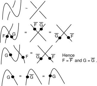
We now examine state summation models constructed given that R=FβŠ—G𝑅tensor-product𝐹𝐺R=F\otimes G as shown in FigureΒ 15. The goal is to show that when we decompose the R𝑅R matrix in this fashion the resulting state summation leads to a trivial invariant. In order to accomplish this aim, we assume that R𝑅R has the form given above, and analyse the effect that this must have on the cup and cap evaluations. This means that we do not actually write cup and cap matrices in doing the analysis. We deduce the form of the invariant from the given conditions, and show that it must be a trivial invariant. Thus we go back to the basic diagrammatic restrictions that are imposed by FigureΒ 10, FigureΒ 11, FigureΒ 12, FigureΒ 13 and deduce conditons that are needed to produce an invariant. This same method of analysis is used throughout the rest of the paper.

Our methods are based on the state summation models for knots and links described in state . In the arguments given below, we assume that a state summation model is given, using this R𝑅R-matrix, and we deduce enough aspects of its structure to conclude that it is a trivial invariant.

From the Yang-Baxter equation as shown in FigureΒ 14, we can deduce the fact that F2=x​Fsuperscript𝐹2π‘₯𝐹F^{2}=xF and G2=t​Gsuperscript𝐺2𝑑𝐺G^{2}=tG. As F𝐹F and G𝐺G are invertible, then F=x​I𝐹π‘₯𝐼F=xI and G=t​I𝐺𝑑𝐼G=tI, where I𝐼I is the identity. Therefore, R=s​I𝑅𝑠𝐼R=sI where s=x​t𝑠π‘₯𝑑s=xt. This fact is also demonstrated in amsshort . We now conclude that R=s​I𝑅𝑠𝐼R=sI and RΒ―=s¯​I¯𝑅¯𝑠𝐼\overline{R}=\overline{s}I, where sΒ―=sβˆ’1¯𝑠superscript𝑠1\overline{s}=s^{-1}. The relations are

⟨[Uncaptioned image]⟩=sΒ―β€‹βŸ¨[Uncaptioned image]⟩delimited-⟨⟩[Uncaptioned image]¯𝑠delimited-⟨⟩[Uncaptioned image]\langle\raisebox{-0.3pt}{\includegraphics[width=17.07182pt,height=14.22636pt]{rcross.eps}}\rangle=\overline{s}\langle\raisebox{-0.25pt}{\includegraphics[width=12.80365pt,height=14.22636pt]{identity.eps}}\rangle
⟨[Uncaptioned image]⟩=sβ€‹βŸ¨[Uncaptioned image]⟩delimited-⟨⟩[Uncaptioned image]𝑠delimited-⟨⟩[Uncaptioned image]\langle\raisebox{-0.3pt}{\includegraphics[width=17.07182pt,height=14.22636pt]{cross.eps}}\rangle=s\langle\raisebox{-0.25pt}{\includegraphics[width=12.80365pt,height=14.22636pt]{identity.eps}}\rangle

We use the following lemmas to construct an invariant from the state summation given by the above relations.

Lemma 3.3

⟨[Uncaptioned image]⟩=s2β€‹βŸ¨[Uncaptioned image]⟩.delimited-⟨⟩[Uncaptioned image]superscript𝑠2delimited-⟨⟩[Uncaptioned image]\langle\raisebox{-0.25pt}{\includegraphics[width=12.80365pt,height=14.22636pt]{identity.eps}}\rangle=s^{2}\langle\raisebox{-0.2pt}{\includegraphics[width=9.95863pt,height=9.95863pt]{capcap.eps}}\rangle.
Proof

Note that the relation

⟨[Uncaptioned image]⟩=⟨[Uncaptioned image]⟩delimited-⟨⟩[Uncaptioned image]delimited-⟨⟩[Uncaptioned image]\langle\raisebox{-0.3pt}{\includegraphics[width=17.07182pt,height=14.22636pt]{rcross.eps}}\rangle=\langle\raisebox{-0.3pt}{\includegraphics[width=17.07182pt,height=14.22636pt]{twist.eps}}\rangle

is independent of the particular choice of cup or cap matrices. This is analogous to twisting R¯¯𝑅\overline{R}. By applying the smoothings associated to R𝑅R and R¯¯𝑅\overline{R}, we arrive at the following:

sΒ―β€‹βŸ¨[Uncaptioned image]⟩=sβ€‹βŸ¨[Uncaptioned image]⟩,¯𝑠delimited-⟨⟩[Uncaptioned image]𝑠delimited-⟨⟩[Uncaptioned image]\overline{s}\langle\raisebox{-0.2pt}{\includegraphics[width=12.80365pt,height=14.22636pt]{identity.eps}}\rangle=s\langle\raisebox{-0.2pt}{\includegraphics[width=18.49411pt,height=12.80365pt]{updownsideside.eps}}\rangle,
sΒ―β€‹βŸ¨[Uncaptioned image]⟩=sβ€‹βŸ¨[Uncaptioned image]⟩,¯𝑠delimited-⟨⟩[Uncaptioned image]𝑠delimited-⟨⟩[Uncaptioned image]\overline{s}\langle\raisebox{-0.2pt}{\includegraphics[width=12.80365pt,height=14.22636pt]{identity.eps}}\rangle=s\langle\raisebox{-0.2pt}{\includegraphics[width=10.81218pt,height=9.95863pt]{capcap.eps}}\rangle,
⟨[Uncaptioned image]⟩=s2β€‹βŸ¨[Uncaptioned image]⟩.delimited-⟨⟩[Uncaptioned image]superscript𝑠2delimited-⟨⟩[Uncaptioned image]\langle\raisebox{-0.25pt}{\includegraphics[width=12.80365pt,height=14.22636pt]{identity.eps}}\rangle=s^{2}\langle\raisebox{-0.2pt}{\includegraphics[width=10.81218pt,height=9.95863pt]{capcap.eps}}\rangle.

∎

Corollary 3.3.1

⟨[Uncaptioned image]⟩=s2β€‹βŸ¨[Uncaptioned image]⟩.delimited-⟨⟩[Uncaptioned image]superscript𝑠2delimited-⟨⟩[Uncaptioned image]\langle\raisebox{-0.25pt}{\includegraphics[width=14.22636pt,height=14.22636pt]{circ.eps}}\rangle=s^{2}\langle\raisebox{-0.2pt}{\includegraphics[width=15.6491pt,height=12.80365pt]{circcirc.eps}}\rangle.

Corollary 3.3.2

⟨[Uncaptioned image]⟩=s2β€‹βŸ¨[Uncaptioned image]⟩.delimited-⟨⟩[Uncaptioned image]superscript𝑠2delimited-⟨⟩[Uncaptioned image]\langle\raisebox{-0.25pt}{\includegraphics[width=14.22636pt,height=14.22636pt]{hcirccirc.eps}}\rangle=s^{2}\langle\raisebox{-0.2pt}{\includegraphics[width=15.6491pt,height=12.80365pt]{pinch.eps}}\rangle.

Setting the value of the circle equal to δ𝛿\delta, we have that δ​s2=1𝛿superscript𝑠21\delta s^{2}=1 and s2=Ξ΄superscript𝑠2𝛿s^{2}=\delta. We now arrive at the fact that s4=1superscript𝑠41s^{4}=1.

Lemma 3.4 (The Second Reidemeister Move) Invariance of the state summation under the second Reidemeister move follows from the formal properties we have given so far.

Proof

By applying our smoothing to the following diagram and then using Lemma 3.3 we get

⟨[Uncaptioned image]⟩=s2β€‹βŸ¨[Uncaptioned image]⟩=⟨[Uncaptioned image]⟩.delimited-⟨⟩[Uncaptioned image]superscript𝑠2delimited-⟨⟩[Uncaptioned image]delimited-⟨⟩[Uncaptioned image]\langle\raisebox{-0.25pt}{\includegraphics[width=14.22636pt,height=14.22636pt]{2ndreid1.eps}}\rangle=s^{2}\langle\raisebox{-0.25pt}{\includegraphics[width=14.22636pt,height=11.38092pt]{capcap.eps}}\rangle=\langle\raisebox{-0.25pt}{\includegraphics[width=14.22636pt,height=14.22636pt]{2ndreid2.eps}}\rangle.

∎

Lemma 3.5 (The Third Reidemeister Move) Invariance of the state summation under the third Reidemeister move follows from the formal properties we have given so far.

Proof

The third Reidemeister move immediately follows by replacing one crossing by a smoothing as shown just before Lemma 3.3, and then using Lemma 3.4. ∎

Lemma 3.6 (The First Reidemeister Move) The state sum multiplies by s𝑠s for positive curls and by s¯¯𝑠\bar{s} for negative curls.

Proof

Since the relations are

⟨[Uncaptioned image]⟩=sΒ―β€‹βŸ¨[Uncaptioned image]⟩,delimited-⟨⟩[Uncaptioned image]¯𝑠delimited-⟨⟩[Uncaptioned image]\langle\raisebox{-0.3pt}{\includegraphics[width=17.07182pt,height=14.22636pt]{rcross.eps}}\rangle=\overline{s}\langle\raisebox{-0.25pt}{\includegraphics[width=12.80365pt,height=14.22636pt]{identity.eps}}\rangle,
⟨[Uncaptioned image]⟩=sβ€‹βŸ¨[Uncaptioned image]⟩,delimited-⟨⟩[Uncaptioned image]𝑠delimited-⟨⟩[Uncaptioned image]\langle\raisebox{-0.3pt}{\includegraphics[width=17.07182pt,height=14.22636pt]{cross.eps}}\rangle=s\langle\raisebox{-0.25pt}{\includegraphics[width=12.80365pt,height=14.22636pt]{identity.eps}}\rangle,

we can apply them to the curls.

⟨[Uncaptioned image]⟩=sβ€‹βŸ¨[Uncaptioned image]⟩=sβ€‹Ξ΄β€‹βŸ¨[Uncaptioned image]⟩=s3β€‹βŸ¨[Uncaptioned image]⟩=sΒ―β€‹βŸ¨[Uncaptioned image]⟩.delimited-⟨⟩[Uncaptioned image]𝑠delimited-⟨⟩[Uncaptioned image]𝑠𝛿delimited-⟨⟩[Uncaptioned image]superscript𝑠3delimited-⟨⟩[Uncaptioned image]¯𝑠delimited-⟨⟩[Uncaptioned image]\langle\raisebox{-0.25pt}{\includegraphics[width=11.38092pt,height=11.38092pt]{loop.eps}}\rangle=s\langle\raisebox{-0.25pt}{\includegraphics[width=11.38092pt,height=11.38092pt]{circline.eps}}\rangle=s\delta\langle\raisebox{-0.2pt}{\includegraphics[width=11.38092pt,height=9.95863pt]{line.eps}}\rangle=s^{3}\langle\raisebox{-0.2pt}{\includegraphics[width=11.38092pt,height=9.95863pt]{line.eps}}\rangle=\overline{s}\langle\raisebox{-0.2pt}{\includegraphics[width=11.38092pt,height=9.95863pt]{line.eps}}\rangle.

The other relation follows in the same fashion. ∎

Theorem 3.2 The quantum state summation given by R=FβŠ—G𝑅tensor-product𝐹𝐺R=F\otimes G is a trivial invariant of unoriented knots.

Proof

In order to get an ambient isotopy invariant fKsubscript𝑓𝐾f_{K} for knots, we would need to compensate for the extra factors that arise from performing the first Reidemeister move. We accomplish this via writhe-normalization as in state . For a knot K𝐾K we define fKsubscript𝑓𝐾f_{K} by the equation

fK=sβˆ’w​(K)β€‹βŸ¨K⟩.subscript𝑓𝐾superscript𝑠𝑀𝐾delimited-⟨⟩𝐾f_{K}=s^{-w(K)}\langle K\rangle.

In order to use this formula, orient the knot diagram and then smooth it in an oriented way at every crossings. The result of this smoothing is the collection of Seifert Circles for the diagram. Let S​C​(K)𝑆𝐢𝐾SC(K) denote the number of Seifert circles in K.𝐾K. Using the results above including the writhe compensation it is easy to see that each crossing contributes s2​s​g​n​(c)superscript𝑠2𝑠𝑔𝑛𝑐s^{2sgn(c)} where s​g​n​(c)𝑠𝑔𝑛𝑐sgn(c) denotes the sign of the crossing. The factor of 222 occurs because both sign of crossing and smoothing of crossing each contribute ss​g​n​(c).superscript𝑠𝑠𝑔𝑛𝑐s^{sgn(c)}. From this it follows that

fK=sβˆ’2​w​r​(K)​δS​C​(K)=Ξ΄βˆ’w​r​(K)+S​C​(K).subscript𝑓𝐾superscript𝑠2π‘€π‘ŸπΎsuperscript𝛿𝑆𝐢𝐾superscriptπ›Ώπ‘€π‘ŸπΎπ‘†πΆπΎf_{K}=s^{-2wr(K)}\delta^{SC(K)}=\delta^{-wr(K)+SC(K)}.

The Lemma in the Appendix to this paper shows that

βˆ’w​r​(K)+S​C​(K)≑1(mod2).π‘€π‘ŸπΎπ‘†πΆπΎannotated1pmod2-wr(K)+SC(K)\equiv 1\pmod{2}.

Therefore, since Ξ΄2=1,superscript𝛿21\delta^{2}=1, we conclude that fK=Ξ΄subscript𝑓𝐾𝛿f_{K}=\delta for all knots K.𝐾K. This completes the proof of the Theorem. ∎

B𝐡\textstyle{B}ΞΌπœ‡\textstyle{\mu}Β Β Β Β Β Β Β Β Β Β Β Β Β Β Β Β Β Β aπ‘Ž\textstyle{a}b𝑏\textstyle{b}i𝑖\textstyle{i}
Figure 16: In braid closures the enhancement operator ΞΌπœ‡\mu must correspond to a cup and a cap.

3.2 The Swap Case

In FigureΒ 17 we show the form of the braiding operator for the unoriented swap case. We begin this section by analyzing the state sum models for operators of this form. For an unoriented knot or link diagram K𝐾K in Morse form, we will let the invariant of regular isotopy associated with this braiding operator be denoted by I​n​v​a​r​(K).πΌπ‘›π‘£π‘Žπ‘ŸπΎInvar(K).

Theorem The state sum model I​n​v​a​r​(K)πΌπ‘›π‘£π‘Žπ‘ŸπΎInvar(K) for K𝐾K in the unoriented swap case produces only trivial invariants for knots (links of one component).

Proof

First note that via FigureΒ 18 we have that the Yang-Baxter equation for R𝑅R implies that F​G=G​F𝐹𝐺𝐺𝐹FG=GF in the swap case where F𝐹F and G𝐺G appear in R𝑅R as in FigureΒ 17. Then from FigureΒ 19 we conclude that FΒ―=F¯𝐹𝐹\overline{F}=F and GΒ―=G¯𝐺𝐺\overline{G}=G so that F2=1=G2.superscript𝐹21superscript𝐺2F^{2}=1=G^{2}. The FigureΒ 19 shows that we can slide F𝐹F and G𝐺G over maxima and minima in the diagram leaving them unchanged. This means that in a knot diagram we can collect all algebra on a diagram as a single product along a given arc. Since the number of F𝐹F’s equals the number of crossings, and the number of G𝐺G’s equals the number of crossings, we have that the algebraic expression can be written in the form Fn​Gnsuperscript𝐹𝑛superscript𝐺𝑛F^{n}G^{n} where n𝑛n is the number of crossings in the knot diagram. Since F2=G2=1,superscript𝐹2superscript𝐺21F^{2}=G^{2}=1, we can take the exponent n𝑛n modulo two. We also know that S≑n+1𝑆𝑛1S\equiv n+1 ( mod 222) where S𝑆S denotes the number of Seifert circuits in the knot diagram. This follows from the Lemma in the Appendix to this paper. Furthermore, the Whitney degree of the underlying plane curve of the diagram is congruent modulo two to S𝑆S FKT . It follows that Fn​Gn=F​Gsuperscript𝐹𝑛superscript𝐺𝑛𝐹𝐺F^{n}G^{n}=FG when the Whitney degree is even and Fn​Gn=Isuperscript𝐹𝑛superscript𝐺𝑛𝐼F^{n}G^{n}=I when the Whitney degree is odd. Taking into account the fact that every Reidemeister type one move contributes 111 to the Whitney degree and contributes F​G𝐹𝐺FG to the algebraic part of the evaluation, we see that the evaluation of any knot diagram is the same as the evaluation of a corresponding unknot diagram with the same writhe and Whitney degree. This completes the proof that the knot invariant cannot distinguish any knot from the unknot. ∎

It remains to discuss the possibility that the invariant could detect a link. For the purpose of this discussion we shall take the cup and cap operators for this model to be identity operators. That is, we shall assume that Ma​b=Ξ΄a​bsubscriptπ‘€π‘Žπ‘subscriptπ›Ώπ‘Žπ‘M_{ab}=\delta_{ab} and Ma​b=Ξ΄a​bsuperscriptπ‘€π‘Žπ‘superscriptπ›Ώπ‘Žπ‘M^{ab}=\delta^{ab} where Ξ΄a​b=Ξ΄a​b=1subscriptπ›Ώπ‘Žπ‘superscriptπ›Ώπ‘Žπ‘1\delta_{ab}=\delta^{ab}=1 if and only if a=bπ‘Žπ‘a=b and Ξ΄a​b=Ξ΄a​b=0subscriptπ›Ώπ‘Žπ‘superscriptπ›Ώπ‘Žπ‘0\delta_{ab}=\delta^{ab}=0 when aβ‰ b.π‘Žπ‘a\neq b. From FigureΒ 20 we see that if the evaluation of a loop of Whitney degree one, labeled with an algebraic expression Ξ±,𝛼\alpha, is denoted by T​r​(Ξ±)π‘‡π‘Ÿπ›ΌTr(\alpha), then the evaluation of the Hopf Link as shown in this figure is T​r​(F​G)​T​r​(F​G)=T​r​(F​G)2.π‘‡π‘ŸπΉπΊπ‘‡π‘ŸπΉπΊπ‘‡π‘Ÿsuperscript𝐹𝐺2Tr(FG)Tr(FG)=Tr(FG)^{2}. The corresponding evaluation of an unlink is T​r​(I)2.π‘‡π‘Ÿsuperscript𝐼2Tr(I)^{2}. We will now give an explicit example for F𝐹F and G𝐺G where these two evaluations differ, showing that an invariant in the unoriented swap case can detect linking even though the Yang-Baxter operator is not entangling. Consider the matrices F𝐹F and G𝐺G shown below.

F=[001010100],G=[1000βˆ’10001],F​G=[0010βˆ’10100].formulae-sequence𝐹delimited-[]001010100formulae-sequence𝐺delimited-[]100010001𝐹𝐺delimited-[]001010100F=\left[\begin{array}[]{ccc}0&0&1\\ 0&1&0\\ 1&0&0\end{array}\right],G=\left[\begin{array}[]{ccc}1&0&0\\ 0&-1&0\\ 0&0&1\end{array}\right],FG=\left[\begin{array}[]{ccc}0&0&1\\ 0&-1&0\\ 1&0&0\end{array}\right].

It is easy to verify that F2=G2=Isuperscript𝐹2superscript𝐺2𝐼F^{2}=G^{2}=I and that F​G=G​F.𝐹𝐺𝐺𝐹FG=GF. The state sum model will use T​r​(Ξ±)=T​r​a​c​e​(Ξ±)π‘‡π‘Ÿπ›Όπ‘‡π‘Ÿπ‘Žπ‘π‘’π›ΌTr(\alpha)=Trace(\alpha) where Trace denotes standard matrix trace. This gives a consistent state model. Note that both F𝐹F and G𝐺G are symmetric matrices and that this corresponds to the invariance of the slide over maxima and minima in FigureΒ 19. We then have (since these are 3Γ—3333\times 3 matrices) that T​r​(I)=3π‘‡π‘ŸπΌ3Tr(I)=3 while T​r​(F​G)=βˆ’1.π‘‡π‘ŸπΉπΊ1Tr(FG)=-1. Thus (T​r​(F​G))2=1superscriptπ‘‡π‘ŸπΉπΊ21(Tr(FG))^{2}=1 while (T​r​(I))2=9superscriptπ‘‡π‘ŸπΌ29(Tr(I))^{2}=9 and so this invariant detects the Hopf Link.

Remark. Note that the result of doing a first Reidemeister move for the invariant under discussion is to multiply the algebra element on the component on which the move occurs by F​G.𝐹𝐺FG. See FigureΒ 21. Since the algebra on a given component is either F​G𝐹𝐺FG or the identity I,𝐼I, we see that the result of a first Reidemeister move is to switch the value of the invariant on this component from T​r​(F​G)=βˆ’1π‘‡π‘ŸπΉπΊ1Tr(FG)=-1 to T​r​(I)=3π‘‡π‘ŸπΌ3Tr(I)=3 or from 333 to βˆ’1.1-1. The simplest way to use the invariant as an invariant of ambient isotopy is to use the fact: Two links with the same Whitney degree and writhe (for each component) are regularly isotopic if and only if they are ambient isotopic. See OnKnots . In this way we can prepare diagrams for comparison. This is how we know that the Hopf Link as shown in FigureΒ 20 is shown to be non-trivial by this invariant. The two components of the Hopf Link diagram used in the calculation give results identical to two disjoint circles for the unlink.

We have the following result:

Theorem The state sum model I​n​v​a​r​(K)πΌπ‘›π‘£π‘Žπ‘ŸπΎInvar(K) for links K𝐾K of two components can detect the modulo two linking number of any link of two components and is non-trivial for links of odd linking number and trivial for links of even linking number.

Proof

The proof follows from the discussion above and an easy analysis of the products of algebra elements that occur on the link components. ∎

Remark. We underline the fact that we have constructed a state sum invariant of knots and links, based on a non-entangling Yang-Baxter operater ( of swap type) that can detect the Hopf Link. This shows that the state sum models in this swap case have a similar relationship with linking and quantum entanglement as do the enhanced Yang-Baxter operators using Markov trace as in Section 3 of amsshort , where an example of the detection of the Hopf link is given in a different way. The state sum that we have described here does not fit into the braiding form with enhanced Yang-Baxter operator that is used in amsshort , but our state sum is indeed based on a Yang-Baxter operator. The examples in both cases show that non-entangling Yang-Baxter operators can detect non-trival topological linking.
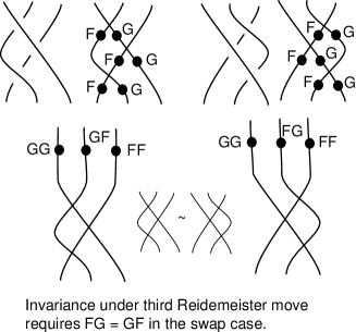
R𝑅\textstyle{R}βˆ™βˆ™\textstyle{\bullet}βˆ™βˆ™\textstyle{\bullet}F𝐹\textstyle{F}G𝐺\textstyle{G}=\textstyle{=} βˆ™βˆ™\textstyle{\bullet}βˆ™βˆ™\textstyle{\bullet}F¯¯𝐹\textstyle{\overline{F}}G¯¯𝐺\textstyle{\overline{G}}=\textstyle{=}R¯¯𝑅\textstyle{\overline{R}}
Figure 17: Topological relations for the swap case.
Refer to caption
Figure 18: Third Reidemeister Move Implies F​G=G​F.𝐹𝐺𝐺𝐹FG=GF.
Refer to caption
Figure 19: Swing Move Implies F​F=G​G=I.𝐹𝐹𝐺𝐺𝐼FF=GG=I.
Refer to caption
Figure 20: Invariant of the Hopf Link.
Refer to caption
Figure 21: Behaviour under a Curl.

We now compare the methods of amsshort and our methods in this swap case. We rely heavily on quantum link invariants in this part of the paper. The decomposition of an R𝑅R matrix in the the swap S∘(FβŠ—G)𝑆tensor-product𝐹𝐺S\circ(F\otimes G) is represented topologically for both R𝑅R and R¯¯𝑅\overline{R} in FigureΒ 17.

The proof in amsshort relies on the use of enhanced Yang-Baxter operators defined below.

Definition 3.7 Let V𝑉V be a finite-dimensional complex Hilbert space, R∈G​L​(VβŠ—V)𝑅𝐺𝐿tensor-product𝑉𝑉R\in GL(V\otimes V) a Yang-Baxter operator, and μ∈E​n​d​(V)πœ‡πΈπ‘›π‘‘π‘‰\mu\in End(V). If R𝑅R commutes with ΞΌβŠ—ΞΌtensor-productπœ‡πœ‡\mu\otimes\mu and

T​r2​(Rβ‹…ΞΌβŠ—ΞΌ)=T​r2​(RΒ―β‹…ΞΌβŠ—ΞΌ)=μ𝑇subscriptπ‘Ÿ2tensor-productβ‹…π‘…πœ‡πœ‡π‘‡subscriptπ‘Ÿ2tensor-productβ‹…Β―π‘…πœ‡πœ‡πœ‡Tr_{2}(R\cdot\mu\otimes\mu)=Tr_{2}(\overline{R}\cdot\mu\otimes\mu)=\mu

then we say that the pair β„›=(R,ΞΌ)β„›π‘…πœ‡\mathcal{R}=(R,\mu) is an enhanced Yang-Baxter operator. In that case, given any braid b𝑏b we define

Iℛ​(b)=T​r​[ρnR​(b)β‹…ΞΌβŠ—n].subscriptπΌβ„›π‘π‘‡π‘Ÿdelimited-[]β‹…superscriptsubscriptπœŒπ‘›π‘…π‘superscriptπœ‡tensor-productabsent𝑛I_{\mathcal{R}}(b)=Tr[\rho_{n}^{R}(b)\cdot\mu^{\otimes n}].

For a braid closure, the enhancement operator is analogous to a product of cup and cap matrices Mb​isuperscript𝑀𝑏𝑖M^{bi} and Ma​isubscriptπ‘€π‘Žπ‘–M_{ai} taking b𝑏b to be a point on the strand at the top of the braid, aπ‘Ža to be the corresponding point on the strand at the bottom of the braid, and i𝑖i to be the point in the middle dividing the cup and the cap. This analogy is shown in FigureΒ 16. Note also that Mb​i=Mb​isuperscript𝑀𝑏𝑖subscript𝑀𝑏𝑖M^{bi}=M_{bi} and Ma​bsuperscriptπ‘€π‘Žπ‘M^{ab} is the inverse of Ma​bsubscriptπ‘€π‘Žπ‘M_{ab}. Therefore, note that ΞΌ=Mb​i​Ma​i=(M​M⊀)a​bπœ‡superscript𝑀𝑏𝑖subscriptπ‘€π‘Žπ‘–subscript𝑀superscript𝑀topπ‘Žπ‘\mu=M^{bi}M_{ai}=(MM^{\top})_{ab}. Given M=(Ma​b)𝑀superscriptπ‘€π‘Žπ‘M=(M^{ab}) is a cup and N=(Ma​b)𝑁subscriptπ‘€π‘Žπ‘N=(M_{ab}) is a cap (they are inverses), in general we have that

M=[abcd],Mβˆ’1=N=1Δ​[dβˆ’bβˆ’ca],formulae-sequence𝑀delimited-[]π‘Žπ‘π‘π‘‘superscript𝑀1𝑁1Ξ”delimited-[]π‘‘π‘π‘π‘ŽM=\left[\begin{array}[]{cc}a&b\\ c&d\end{array}\right],\qquad M^{-1}=N=\frac{1}{\Delta}\left[\begin{array}[]{cc}d&-b\\ -c&a\end{array}\right],

with Ξ”=a​dβˆ’b​cΞ”π‘Žπ‘‘π‘π‘\Delta=ad-bc as M𝑀M and N𝑁N must be inverses of one another. Thus

ΞΌ=(M​N⊀)a​b=1Δ​[abcd]​[dβˆ’cβˆ’ba]=1Δ​[a​dβˆ’b2βˆ’a​c+a​bc​dβˆ’b​dβˆ’c2+a​d].πœ‡subscript𝑀superscript𝑁topπ‘Žπ‘1Ξ”delimited-[]π‘Žπ‘π‘π‘‘delimited-[]π‘‘π‘π‘π‘Ž1Ξ”delimited-[]π‘Žπ‘‘superscript𝑏2π‘Žπ‘π‘Žπ‘π‘π‘‘π‘π‘‘superscript𝑐2π‘Žπ‘‘\mu=(MN^{\top})_{ab}=\frac{1}{\Delta}\left[\begin{array}[]{cc}a&b\\ c&d\end{array}\right]\left[\begin{array}[]{cc}d&-c\\ -b&a\end{array}\right]=\frac{1}{\Delta}\left[\begin{array}[]{cc}ad-b^{2}&-ac+ab\\ cd-bd&-c^{2}+ad\end{array}\right].

In amsshort , the authors found the following invertible ΞΌπœ‡\mu for constructing an invariant. We will show that this ΞΌπœ‡\mu cannot be obtained by the cup and cap construction. (It is also the case that in amsshort non-invertible ΞΌπœ‡\mu are considered and shown to be unnecessary, but that is not the issue here.)

ΞΌ=[100βˆ’1].πœ‡delimited-[]1001\mu=\left[\begin{array}[]{cc}1&0\\ 0&-1\end{array}\right].

If we try to set our derivation of ΞΌπœ‡\mu from cup and cap operators equal to theirs, we then get matrix solutions that have a determinant of zero.

a​dβˆ’b2=Ξ”,βˆ’a​c+a​b=0,c​dβˆ’b​d=0,c2βˆ’a​d=Ξ”.π‘Žπ‘‘superscript𝑏2Ξ”π‘Žπ‘π‘Žπ‘0𝑐𝑑𝑏𝑑0superscript𝑐2π‘Žπ‘‘Ξ”\begin{array}[]{rcl}ad-b^{2}&=&\Delta,\\ -ac+ab&=&0,\\ cd-bd&=&0,\\ c^{2}-ad&=&\Delta.\end{array}

Solving the above system of equations implies that d=c2a𝑑superscript𝑐2π‘Žd=\frac{c^{2}}{a}, which makes the determinant of the matrix zero. Therefore, in general we cannot extend the models used in amsshort to quantum link invariants. This shows that we cannot always construct an analogous state summation model for the unoriented swap case. Nevertheless, we have shown that all properties relative to non-entangling Yang-Baxter operators happen in the same way in both of these categories of invariants.

Remark 3.8 We believe this is the first time an explicit difference has been shown between the Markov trace and state summation methods of constructing invariants.

4 Oriented State Models Given by Non-Entangling Operators

We now express the above arguments in the oriented case for quantum invariant state summations. The results of amsshort generalize easily in this case. See stat for an account of oriented state sum models for link invariants, based on solutions to the Yang-Baxter equation. These models are essentially the same as the unoriented models, but have orientations associated with the crossings, cups, and caps. We begin with the simple product decomposition of R𝑅R.

4.1 The Product Case

Theorem 4.1 The state summation model given by R=FβŠ—G𝑅tensor-product𝐹𝐺R=F\otimes G is trivial for oriented knots.

Proof

For the oriented product case, we begin with the following equations, as given in Section 3:

⟨[Uncaptioned image]⟩=sβ€‹βŸ¨[Uncaptioned image]⟩,delimited-⟨⟩[Uncaptioned image]𝑠delimited-⟨⟩[Uncaptioned image]\langle\raisebox{-0.2pt}{\includegraphics[width=14.22636pt,height=11.38092pt]{crossorient.eps}}\rangle=s\langle\raisebox{-0.2pt}{\includegraphics[width=14.22636pt,height=14.22636pt]{identityorient.eps}}\rangle,
⟨[Uncaptioned image]⟩=sΒ―β€‹βŸ¨[Uncaptioned image]⟩.delimited-⟨⟩[Uncaptioned image]¯𝑠delimited-⟨⟩[Uncaptioned image]\langle\raisebox{-0.2pt}{\includegraphics[width=14.22636pt,height=11.38092pt]{rcrossorient.eps}}\rangle=\overline{s}\langle\raisebox{-0.2pt}{\includegraphics[width=14.22636pt,height=14.22636pt]{identityorient.eps}}\rangle.

We find the value of the loop by examining how the model behaves on the oriented curls. We apply our oriented smoothing relations to determine what factors arise from each curl:

⟨[Uncaptioned image]⟩=sΒ―β€‹βŸ¨[Uncaptioned image]⟩=sΒ―β€‹Ξ΄β€‹βŸ¨[Uncaptioned image]⟩delimited-⟨⟩[Uncaptioned image]¯𝑠delimited-⟨⟩[Uncaptioned image]¯𝑠𝛿delimited-⟨⟩[Uncaptioned image]\langle\raisebox{-0.2pt}{\includegraphics[width=12.80365pt,height=12.80365pt]{orientloop.eps}}\rangle=\overline{s}\langle\raisebox{-0.2pt}{\includegraphics[width=12.80365pt,height=12.80365pt]{orientloopline.eps}}\rangle=\overline{s}\delta\langle\raisebox{-0.2pt}{\includegraphics[width=12.80365pt,height=12.80365pt]{lineorient.eps}}\rangle
⟨[Uncaptioned image]⟩=sβ€‹βŸ¨[Uncaptioned image]⟩=sβ€‹Ξ΄β€‹βŸ¨[Uncaptioned image]⟩,delimited-⟨⟩[Uncaptioned image]𝑠delimited-⟨⟩[Uncaptioned image]𝑠𝛿delimited-⟨⟩[Uncaptioned image]\langle\raisebox{-0.2pt}{\includegraphics[width=12.80365pt,height=12.80365pt]{reverseorient.eps}}\rangle=s\langle\raisebox{-0.2pt}{\includegraphics[width=12.80365pt,height=12.80365pt]{orientloopline.eps}}\rangle=s\delta\langle\raisebox{-0.2pt}{\includegraphics[width=12.80365pt,height=12.80365pt]{lineorient.eps}}\rangle,

taking δ𝛿\delta to be the value of the oriented loop. In order to satisfy the relation ⟨[Uncaptioned image]⟩=⟨[Uncaptioned image]⟩delimited-⟨⟩[Uncaptioned image]delimited-⟨⟩[Uncaptioned image]\langle\raisebox{-0.2pt}{\includegraphics[width=22.76228pt,height=12.80365pt]{doubleorientloop.eps}}\rangle=\langle\raisebox{-0.2pt}{\includegraphics[width=12.80365pt,height=12.80365pt]{lineorient.eps}}\rangle we need that (s¯​δ)​(s​δ)=Ξ΄2=1¯𝑠𝛿𝑠𝛿superscript𝛿21(\overline{s}\delta)(s\delta)=\delta^{2}=1. Thus, the absolute value of an oriented loop is equal to one. To construct a model that is invariant under Reidemeister I we must multiply by a writhe corrective factor, so our final invariant has the form

fk=(s​δ)βˆ’w​(K)β€‹βŸ¨K⟩,subscriptπ‘“π‘˜superscript𝑠𝛿𝑀𝐾delimited-⟨⟩𝐾f_{k}=(s\delta)^{-w(K)}\langle K\rangle,

as s​δ𝑠𝛿s\delta is the value that comes from using our oriented smoothing relations on a positive writhe looped strand.

Note that if K𝐾K is a given diagram, then we have an explicit formula for ⟨K⟩delimited-⟨⟩𝐾\langle K\rangle via smoothing in an oriented way at each crossing. The result of this smoothing is the set of Seifert circles for the diagram weighted by s𝑠s or s¯¯𝑠\overline{s} at each smoothing site. Thus the evaluation is given by the formula

⟨K⟩=sw​(K)​δS​Cβˆ’1.delimited-⟨⟩𝐾superscript𝑠𝑀𝐾superscript𝛿𝑆𝐢1\langle K\rangle=s^{w(K)}\delta^{SC-1}.

Substituting,

fk=(s​δ)βˆ’w​(K)β€‹βŸ¨K⟩=sβˆ’w​(K)​sw​(K)β€‹Ξ΄βˆ’w​(K)​δS​Cβˆ’1=Ξ΄S​Cβˆ’w​(K)βˆ’1.subscriptπ‘“π‘˜superscript𝑠𝛿𝑀𝐾delimited-⟨⟩𝐾superscript𝑠𝑀𝐾superscript𝑠𝑀𝐾superscript𝛿𝑀𝐾superscript𝛿𝑆𝐢1superscript𝛿𝑆𝐢𝑀𝐾1f_{k}=(s\delta)^{-w(K)}\langle K\rangle=s^{-w(K)}s^{w(K)}\delta^{-w(K)}\delta^{SC-1}=\delta^{SC-w(K)-1}.

Here, S​C𝑆𝐢SC stands for the number of Seifert circles produced from an oriented link diagram. If Ξ΄=1𝛿1\delta=1 then the invariant is trivial. We now show that the invariant is still trivial for βˆ’11-1 regardless of the number of Seifert circles or the writhe. To do this we show that the number of Seifert circles minus the writhe of the knot is always odd. Notice that the unknot has one Seifert circle and no writhe, so fu​n​k​n​o​t=Ξ΄1βˆ’0βˆ’1=Ξ΄0=1subscriptπ‘“π‘’π‘›π‘˜π‘›π‘œπ‘‘superscript𝛿101superscript𝛿01f_{unknot}=\delta^{1-0-1}=\delta^{0}=1. Similarly, note that the trefoil knot with w​(K)=+3𝑀𝐾3w(K)=+3 produces two Seifert circles, so ft​r​e​f​o​i​l=Ξ΄2βˆ’3βˆ’1=Ξ΄βˆ’2=+1subscriptπ‘“π‘‘π‘Ÿπ‘’π‘“π‘œπ‘–π‘™superscript𝛿231superscript𝛿21f_{trefoil}=\delta^{2-3-1}=\delta^{-2}=+1. The only question that concerns us is to prove the congruence

S​Cβˆ’w​(K)βˆ’1≑0(mod2),𝑆𝐢𝑀𝐾1annotated0pmod2SC-w(K)-1\equiv 0\pmod{2},

holds for all cases. This is implied by the Lemma in the Appendix to this paper.

Therefore, S​Cβˆ’w​(K)βˆ’1𝑆𝐢𝑀𝐾1SC-w(K)-1 is always even and

fk=Ξ΄S​Cβˆ’w​(K)βˆ’1=(Β±1)S​Cβˆ’w​(K)βˆ’1=1,subscriptπ‘“π‘˜superscript𝛿𝑆𝐢𝑀𝐾1superscriptplus-or-minus1𝑆𝐢𝑀𝐾11f_{k}=\delta^{SC-w(K)-1}=(\pm 1)^{SC-w(K)-1}=1,

thus the invariant is trivial. ∎

4.2 The Swap Case
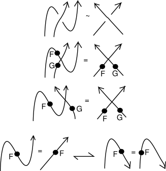
Refer to caption
Figure 22: Oriented Swing Move Implies Algebraic Moveability.

Theorem 4.2 The state summation model given by R=(FβŠ—G)∘S𝑅tensor-product𝐹𝐺𝑆R=(F\otimes G)\circ S is trivial for oriented knots.

Proof

We use the relationship given in FigureΒ 17 and FigureΒ 18 except with orientation going upward such that the arrows are on the top endpoints. By using this decomposition of the Yang-Baxter equation, we arrive at the fact that F​G=G​F𝐹𝐺𝐺𝐹FG=GF (see FigureΒ 18). View FigureΒ 22 and note that it follows that algebra elements can be moved along the lines of the diagram and collected on a single arc, as we saw in the previous unoriented swap case. (We have indicated one case of a number of cases that are verified in the same way.) We also know that F​G=G​F𝐹𝐺𝐺𝐹FG=GF and so we can intrepret this freedom by saying that for each crossing we can remove either F​G𝐹𝐺FG or F¯​G¯¯𝐹¯𝐺\overline{F}\overline{G} and collect it directly to an algebra product that we accumulate from the crossing of the diagram. We can remove them from the diagram itself and write that ⟨[Uncaptioned image]⟩=F​Gβ€‹βŸ¨[Uncaptioned image]⟩delimited-⟨⟩[Uncaptioned image]𝐹𝐺delimited-⟨⟩[Uncaptioned image]\langle\raisebox{-0.2pt}{\includegraphics[width=14.22636pt,height=14.22636pt]{crossorient.eps}}\rangle=FG\langle\raisebox{-0.2pt}{\includegraphics[width=14.22636pt,height=14.22636pt]{swapcrosso.eps}}\rangle. For each R𝑅R we then have an F​G𝐹𝐺FG and for each R¯¯𝑅\overline{R} we have an F¯​G¯¯𝐹¯𝐺\overline{F}\overline{G}. Note that an oriented R¯¯𝑅\overline{R} has a writhe of +11+1. Therefore, we have that

⟨[Uncaptioned image]⟩=F​GΒ―β€‹βŸ¨[Uncaptioned image]⟩.delimited-⟨⟩[Uncaptioned image]¯𝐹𝐺delimited-⟨⟩[Uncaptioned image]\langle\raisebox{-0.2pt}{\includegraphics[width=14.22636pt,height=14.22636pt]{orientloop.eps}}\rangle=\overline{FG}\langle\raisebox{-0.2pt}{\includegraphics[width=14.22636pt,height=14.22636pt]{lineorient.eps}}\rangle.

For each positive writhe loop we output a F​G¯¯𝐹𝐺\overline{FG}. Our invariant has the form fK=(F​G)w​(K)​(F​G)Nβˆ’Psubscript𝑓𝐾superscript𝐹𝐺𝑀𝐾superscript𝐹𝐺𝑁𝑃f_{K}=(FG)^{w(K)}(FG)^{N-P} where P𝑃P is the number of oriented R¯¯𝑅\overline{R} crossings and N𝑁N is the number of oriented R𝑅R crossings. As all oriented R¯¯𝑅\overline{R} and R𝑅R crossings have writhe +11+1 and writhe βˆ’11-1 respectively, this invariant becomes trivial as both (F​G)w​(K)superscript𝐹𝐺𝑀𝐾(FG)^{w(K)} and (F​G)Nβˆ’Psuperscript𝐹𝐺𝑁𝑃(FG)^{N-P} cancel each other out. ∎

5 The Jones Polynomial and Quantum Computation

We now review quantumcompute which gives a local unitary representation that can be used to compute the Jones polynomial Jones ; Jones1 ; Jones2 ; Jones3 ; Jones4 for closures of 3-braids. The quantum computation devolves into finding the trace of a unitary transformation. The result of this construction is a quantum computational model for the Jones polynomial evaluation on a significant class of knots and links that is not involved with quantum entanglement since the unitary transformations are in S​U​(2).π‘†π‘ˆ2SU(2). This result is very interesting to us, even though it is a special case. We do not know how to obtain the Jones polynomial for all knots and links in this way, avoiding entangling operators. The model given here, can be extended to the well-known Fibonacci model qdeformed for quantum computing, but then the transformations are in other unitary groups, and it remains to analyse the full role of quantum entanglement in these generalizations.

The idea behind this construction depends upon the algebra generated by two single qubit density matrices (ket-bras). Let |v⟩ket𝑣\ket{v} and |w⟩ket𝑀\ket{w} be two qubits in V𝑉V, a complex vector space of dimension two over the complex numbers. Let P=|vβŸ©β€‹βŸ¨v|𝑃ket𝑣bra𝑣P=\ket{v}\bra{v} and Q=|wβŸ©β€‹βŸ¨w|𝑄ket𝑀bra𝑀Q=\ket{w}\bra{w} be the corresponding ket-bras. Note that as

P2=|v|2​P,superscript𝑃2superscript𝑣2𝑃P^{2}=|v|^{2}P,
Q2=|w|2​Q,superscript𝑄2superscript𝑀2𝑄Q^{2}=|w|^{2}Q,
P​Q​P=|⟨v|w⟩|2​P,𝑃𝑄𝑃superscriptinner-product𝑣𝑀2𝑃PQP=|\braket{v}{w}|^{2}P,
Q​P​Q=|⟨v|w⟩|2​Q.𝑄𝑃𝑄superscriptinner-product𝑣𝑀2𝑄QPQ=|\braket{v}{w}|^{2}Q.

P𝑃P and Q𝑄Q generate a representation of the Temperley-Lieb algebra. One can adjust parameters to to make a representation of the 3-strand braid group in the form

s1β†’r​P+s​I,β†’subscript𝑠1π‘Ÿπ‘ƒπ‘ πΌs_{1}\rightarrow rP+sI,
s2β†’t​Q+u​I,β†’subscript𝑠2𝑑𝑄𝑒𝐼s_{2}\rightarrow tQ+uI,

where I𝐼I is the identity mapping on V𝑉V and r,s,t,uπ‘Ÿπ‘ π‘‘π‘’r,s,t,u are suitably chosen scalars. In the following, we use this method to adjust such a representation so that it is unitary. Note also that this is a local unitary representation of B3subscript𝐡3B_{3} to U​(2)π‘ˆ2U(2). We leave it as an exercise for the reader to verify that it fits into the general classification of such representations as given in May .

The representation depends on two symmetric but non-unitary matrices U1subscriptπ‘ˆ1U_{1} and U2subscriptπ‘ˆ2U_{2} with

U1=[d000]=d​|wβŸ©β€‹βŸ¨w|,subscriptπ‘ˆ1delimited-[]𝑑000𝑑ket𝑀bra𝑀U_{1}=\left[\begin{array}[]{cc}d&0\\ 0&0\end{array}\right]=d\ket{w}\bra{w},
U2=[dβˆ’11βˆ’dβˆ’21βˆ’dβˆ’2dβˆ’dβˆ’1]=d​|vβŸ©β€‹βŸ¨v|,subscriptπ‘ˆ2delimited-[]superscript𝑑11superscript𝑑21superscript𝑑2𝑑superscript𝑑1𝑑ket𝑣bra𝑣U_{2}=\left[\begin{array}[]{cc}d^{-1}&\sqrt{1-d^{-2}}\\ \sqrt{1-d^{-2}}&d-d^{-1}\end{array}\right]=d\ket{v}\bra{v},

where w=(1,0)𝑀10w=(1,0), and v=(dβˆ’1,1βˆ’dβˆ’2)𝑣superscript𝑑11superscript𝑑2v=(d^{-1},\sqrt{1-d^{-2}}), assuming the entries of v𝑣v are real. Note that U12=d​U1subscriptsuperscriptπ‘ˆ21𝑑subscriptπ‘ˆ1U^{2}_{1}=dU_{1} and U22=d​U1subscriptsuperscriptπ‘ˆ22𝑑subscriptπ‘ˆ1U^{2}_{2}=dU_{1}. Moreover, U1​U2​U1=U1subscriptπ‘ˆ1subscriptπ‘ˆ2subscriptπ‘ˆ1subscriptπ‘ˆ1U_{1}U_{2}U_{1}=U_{1} and U2​U1​U2=U1subscriptπ‘ˆ2subscriptπ‘ˆ1subscriptπ‘ˆ2subscriptπ‘ˆ1U_{2}U_{1}U_{2}=U_{1}. This is an example of a specific representation of the Temperley-Lieb algebra. The desired representation of the Artin braid group is given on the two braid generators for the 3-strand braid group by the equations:

Φ​(s1)=A​I+Aβˆ’1​U1,Ξ¦subscript𝑠1𝐴𝐼superscript𝐴1subscriptπ‘ˆ1\Phi(s_{1})=AI+A^{-1}U_{1},
Φ​(s2)=A​I+Aβˆ’1​U2,Ξ¦subscript𝑠2𝐴𝐼superscript𝐴1subscriptπ‘ˆ2\Phi(s_{2})=AI+A^{-1}U_{2},

where I𝐼I denotes the 2Γ—2222\times 2 identity matrix.

For any A𝐴A with d=βˆ’A2βˆ’Aβˆ’2𝑑superscript𝐴2superscript𝐴2d=-A^{2}-A^{-2} these formulas define a representation of the braid group. With A=ei​θ𝐴superscriptπ‘’π‘–πœƒA=e^{i\theta}, we have d=βˆ’2​cos⁑(2​θ)𝑑22πœƒd=-2\cos(2\theta). One finds a specific range of angles ΞΈπœƒ\theta in the following disjoint union of angular intervals

θ∈[0,Ο€/6]βŠ”[Ο€/3,2​π/3]βŠ”[5​π/6,7​π/6]βŠ”[4​π/3,5​π/3]βŠ”[11​π/6,2​π]πœƒsquare-union0πœ‹6πœ‹32πœ‹35πœ‹67πœ‹64πœ‹35πœ‹311πœ‹62πœ‹\theta\in[0,\pi/6]\sqcup[\pi/3,2\pi/3]\sqcup[5\pi/6,7\pi/6]\sqcup[4\pi/3,5\pi/3]\sqcup[11\pi/6,2\pi]

that give unitary representations of the 3-strand braid group. Thus, a specialization of a more general representation of the braid group gives rise to a continuous family of unitary representations of the braid group.

Note that the traces of these matrices are given by the formulas T​r​(U1)=T​r​(U2)=dπ‘‡π‘Ÿsubscriptπ‘ˆ1π‘‡π‘Ÿsubscriptπ‘ˆ2𝑑Tr(U_{1})=Tr(U_{2})=d while T​r​(U1​U2)=T​r​(U2​U1)=1π‘‡π‘Ÿsubscriptπ‘ˆ1subscriptπ‘ˆ2π‘‡π‘Ÿsubscriptπ‘ˆ2subscriptπ‘ˆ11Tr(U_{1}U_{2})=Tr(U_{2}U_{1})=1. If b𝑏b is any braid, let I​(b)𝐼𝑏I(b) denote the sum of the exponents in the braid word that expresses b𝑏b. For b𝑏b a 3-strand braid, it follows that

Φ​(b)=AI​(b)​I+Π​(b),Φ𝑏superscript𝐴𝐼𝑏𝐼Π𝑏\Phi(b)=A^{I(b)}I+\Pi(b),

where I𝐼I is the 2Γ—2222\times 2 identity matrix and Π​(b)Π𝑏\Pi(b) is a sum of products in the Temperley-Lieb algebra involving U1subscriptπ‘ˆ1U_{1} and U2subscriptπ‘ˆ2U_{2}. Since the Temperley-Lieb algebra in this dimension is generated by I,U1,U2,U1​U2,𝐼subscriptπ‘ˆ1subscriptπ‘ˆ2subscriptπ‘ˆ1subscriptπ‘ˆ2I,U_{1},U_{2},U_{1}U_{2}, and U2​U1subscriptπ‘ˆ2subscriptπ‘ˆ1U_{2}U_{1}, it follows that the value of the bracket polynomial of the closure of the braid b𝑏b, denoted ⟨b¯⟩delimited-βŸ¨βŸ©Β―π‘\langle\overline{b}\rangle, can be calculated directly from the trace of this representation, except for the part involving the identity matrix. The bracket polynomial evaluation depends upon the loop counts in the states of the closure of the braid, and these loop counts correspond to the traces of the non-identity Temperley-Lieb algebra elements. Note that the closure of the 3-strand diagram for the identity braid in B3subscript𝐡3B_{3} has bracket polynomial d2superscript𝑑2d^{2}. The result is the equation

⟨b¯⟩=AI​(b)​d2+T​r​(Π​(b)),delimited-βŸ¨βŸ©Β―π‘superscript𝐴𝐼𝑏superscript𝑑2π‘‡π‘ŸΞ π‘\langle\overline{b}\rangle=A^{I(b)}d^{2}+Tr(\Pi(b)),

where b¯¯𝑏\overline{b} denotes the standard braid closure of b𝑏b, and the sharp brackets denote the bracket polynomial. Since the trace of the 2Γ—2222\times 2 identity matrix is 222, we see that

⟨b¯⟩=T​r​(Φ​(b))+AI​(b)​(d2βˆ’2).delimited-βŸ¨βŸ©Β―π‘π‘‡π‘ŸΞ¦π‘superscript𝐴𝐼𝑏superscript𝑑22\langle\overline{b}\rangle=Tr(\Phi(b))+A^{I(b)}(d^{2}-2).

It follows from this calculation that the question of computing the bracket polynomial for the closure of the 3-strand braid b𝑏b is mathematically equivalent to the problem of computing the trace of the unitary matrix Φ​(b)Φ𝑏\Phi(b). Therefore, we can define topological invariants from quantum situations that lack any sort of entanglement at all as this calculation depends solely on a single qubit.

By using the method we have described in this section, we show that there is indeed a disparity between topological entanglement and entangling quantum gates. Once we leave the Yang-Baxter formalism it is possible to construct strong topological invariants from non-entangling quantum gates. This phenomena needs further exploration, particularly in regard to the Fibonacci model qdeformed and fibonacci

6 Bracket Quantum Link Invariants and Quantum Entanglement

Recall that our cup and cap matrices are given by the following matrix in the unoriented case:

M=[0i​Aβˆ’i​Aβˆ’10].𝑀delimited-[]0𝑖𝐴𝑖superscript𝐴10M=\left[\begin{array}[]{cc}0&iA\\ -iA^{-1}&0\end{array}\right].

Moreover, the bracket relation in state can be given in terms of quantum link invariants as follows

Rc​da​b=A​Ma​b​Mc​d+Aβˆ’1​δca​δdb.subscriptsuperscriptπ‘…π‘Žπ‘π‘π‘‘π΄superscriptπ‘€π‘Žπ‘subscript𝑀𝑐𝑑superscript𝐴1subscriptsuperscriptπ›Ώπ‘Žπ‘subscriptsuperscript𝛿𝑏𝑑R^{ab}_{cd}=AM^{ab}M_{cd}+A^{-1}\delta^{a}_{c}\delta^{b}_{d}.

By substituting in our cup/cap matrix and the 2Γ—2222\times 2 identity matrix we can give an explicit R𝑅R as

R=[Aβˆ’10000Aβˆ’1βˆ’A3A00A00000Aβˆ’1].𝑅delimited-[]superscript𝐴10000superscript𝐴1superscript𝐴3𝐴00𝐴00000superscript𝐴1R=\left[\begin{array}[]{cccc}A^{-1}&0&0&0\\ 0&A^{-1}-A^{3}&A&0\\ 0&A&0&0\\ 0&0&0&A^{-1}\end{array}\right].

In order for R𝑅R to be unitary, note that (Aβˆ’1βˆ’A3)​Aβˆ’1=0superscript𝐴1superscript𝐴3superscript𝐴10(A^{-1}-A^{3})A^{-1}=0 or alternatively 1=A41superscript𝐴41=A^{4}. Therefore, choosing A=Β±i𝐴plus-or-minus𝑖A=\pm i gives us a unitary, invertible matrix. However, given these choices of A𝐴A the matrix becomes unentangling as a matrix of the form

R=[a00000d00c00000b]𝑅delimited-[]π‘Ž00000𝑑00𝑐00000𝑏R=\left[\begin{array}[]{cccc}a&0&0&0\\ 0&0&d&0\\ 0&c&0&0\\ 0&0&0&b\end{array}\right]

is only entangling when a​bβ‰ c​dπ‘Žπ‘π‘π‘‘ab\neq cd as shown in notsoshort . There is, therefore, no R𝑅R matrix solution to the bracket that can be an entangling operator.

7 Virtual Knot Theory and Quantum Entanglement

Take the matrix given below:

R=[000A0Aβˆ’10000Aβˆ’10A000],𝑅delimited-[]000𝐴0superscript𝐴10000superscript𝐴10𝐴000R=\left[\begin{array}[]{cccc}0&0&0&A\\ 0&A^{-1}&0&0\\ 0&0&A^{-1}&0\\ A&0&0&0\end{array}\right],

where A∈S1𝐴superscript𝑆1A\in S^{1} and R𝑅R is unitary and a solution to the Yang-Baxter equation. We now show that R𝑅R is an entangling matrix. Take a decomposed state

|ψ⟩=(x​|0⟩+y​|1⟩)βŠ—(z​|0⟩+w​|1⟩)=x​z​|00⟩+y​z​|10⟩+x​w​|01⟩+y​w​|11⟩.ketπœ“tensor-productπ‘₯ket0𝑦ket1𝑧ket0𝑀ket1π‘₯𝑧ket00𝑦𝑧ket10π‘₯𝑀ket01𝑦𝑀ket11\ket{\psi}=(x\ket{0}+y\ket{1})\otimes(z\ket{0}+w\ket{1})=xz\ket{00}+yz\ket{10}+xw\ket{01}+yw\ket{11}.

Now, we apply R𝑅R to |ψ⟩ketπœ“\ket{\psi} to get

R​|ψ⟩=x​z​A​|11⟩+y​z​Aβˆ’1​|10⟩+x​w​Aβˆ’1​|01⟩+y​w​A​|00⟩.𝑅ketπœ“π‘₯𝑧𝐴ket11𝑦𝑧superscript𝐴1ket10π‘₯𝑀superscript𝐴1ket01𝑦𝑀𝐴ket00R\ket{\psi}=xzA\ket{11}+yzA^{-1}\ket{10}+xwA^{-1}\ket{01}+ywA\ket{00}.

From our definition of entanglement, we take the determinant of the resultant state

det[A​y​wAβˆ’1​x​wy​z​Aβˆ’1x​z​A]=x​y​z​w​(A2βˆ’Aβˆ’2).delimited-[]𝐴𝑦𝑀superscript𝐴1π‘₯𝑀𝑦𝑧superscript𝐴1π‘₯𝑧𝐴π‘₯𝑦𝑧𝑀superscript𝐴2superscript𝐴2\det\left[\begin{array}[]{cc}Ayw&A^{-1}xw\\ yzA^{-1}&xzA\end{array}\right]=xyzw(A^{2}-A^{-2}).

We must have that A=ei​θ𝐴superscriptπ‘’π‘–πœƒA=e^{i\theta}, which implies that

A2βˆ’Aβˆ’2=e2​iβ€‹ΞΈβˆ’eβˆ’2​i​θ=cos⁑(2​θ)+i​sin⁑(2​θ)βˆ’cos⁑(2​θ)+i​sin⁑(2​θ)=2​i​sin⁑(2​θ),superscript𝐴2superscript𝐴2superscript𝑒2π‘–πœƒsuperscript𝑒2π‘–πœƒmissing-subexpression2πœƒπ‘–2πœƒ2πœƒπ‘–2πœƒmissing-subexpression2𝑖2πœƒ\begin{array}[]{rcl}A^{2}-A^{-2}&=&e^{2i\theta}-e^{-2i\theta}\\ &=&\cos(2\theta)+i\sin(2\theta)-\cos(2\theta)+i\sin(2\theta)\\ &=&2i\sin(2\theta),\end{array}

which shows that sin⁑(2​θ)β‰ 02πœƒ0\sin(2\theta)\neq 0. Therefore, there are a continuum of solutions such that this given R𝑅R matrix is entangling. In virtual , R𝑅R is shown to only detect the writhe of classical knots; however, when R𝑅R is applied to virtual knots it is a much stronger invariant. Many of the arguments of this paper can be generalized to virtual knots. Moreover, the relationship between physics and virtual knots has yet to be explored in detail. For quantum computing, the virtual crossing can be modeled as a swap gate (interchange qubits as in S|01⟩=|10⟩)S\ket{01}=\ket{10}). Thus it is natural to use the virtual braid group and its unitary representations for quantum computing. We will return to this subject in a subsequent paper.

8 Topological Entanglement and Quantum Entanglement

In this paper we have, so far, discussed topological entanglement and quantum entanglement by examining quantum operators that are solutions to the Yang-Baxter equation. The operators R𝑅R that we have considered are unitary solutions to the Yang-Baxter equation that act of the tensor product of a single qubit space V𝑉V with itself. Such an operator R:VβŠ—V⟢VβŠ—V:π‘…βŸΆtensor-product𝑉𝑉tensor-product𝑉𝑉R:V\otimes V\longrightarrow V\otimes V can be an entangling operator in the quantum sense. We have shown in this paper that such operators will not produce non-trivial invariants of knots and links (except in very special cases) unless they are quantum entangling. This establishes a connection between the ability to detect topological entanglement and entangled quantum states.

In this section of the paper we discuss more generally the theme of quantum entanglement and topological entanglement. We begin with the Aravind hypothesis Ara . The Aravind hypothesis suggests that topological linking may be directly comparable to quantum entanglement. We discuss the pros and cons of this hypothesis below. The main work of this paper shows that there is a relationship between quantum entangling operators and invariants of knots and links. The Aravind hypothesis suggests that there may be a more direct relationhip of topological and quantum entanglement.

We then discuss the relationship of space, spacetime and quantum entanglement in the context of the a hypothesis of Susskind and Malcedena ER . This E​R=E​P​R𝐸𝑅𝐸𝑃𝑅ER=EPR hypothesis is based on the suggestion that the connectivity of spacetime is a phenomenon of quantum entanglement. Susskind asserts that the entanglement of distant particles is equivalent to the existence of an Einstein-Rosen bridge connecting them. If this hypothesis is true, then there is indeed a topological underpinning for quantum entanglement. Here we will only make foundational comments on the E​R=E​P​R𝐸𝑅𝐸𝑃𝑅ER=EPR hypothesis. In the discussion below we examine entanglement and teleportation in relation to the construction of a that is space augmented by quantum states. Since an entangled state such as |δ⟩=12​(|01⟩+|10⟩)ket𝛿12ket01ket10|\delta\rangle=\frac{1}{\sqrt{2}}(|01\rangle+|10\rangle) is formulated without any background space, we point out that it is possible graphically to form a new space from the given space or spactime S𝑆S of the physics by attaching a corresponding quantum network to S.𝑆S. The new space Sβ€²superscript𝑆′S^{\prime} has connectivity related to the entanglement. This construction can then be considered as a precursor to the spacetime with an Einstein-Rosen bridge connecting the sites of the entangled particles.

8.1 The Aravind Hyppothesis

Link diagrams can be used as holders of information. Aravind Ara proposed that the topological entanglement of a link should correspond to the quantum entanglement of a state. Each link component would correspond to a tensor factor of the state. Measurement of a link would be modeled by deleting one component of the link. A key example is the Borommean rings. See FigureΒ 23. Deleting any component of the Boromean rings yields a remaining pair of unlinked rings. The three Borromean rings are entangled, but any two of them are unentangled. In this sense the Borromean rings are analogous to the G​H​Z𝐺𝐻𝑍GHZ state |G​H​Z⟩=(1/2)​(|000⟩+|111⟩)ket𝐺𝐻𝑍12ket000ket111|GHZ\rangle=(1/\sqrt{2})(|000\rangle+|111\rangle). Measurement in any factor of the G​H​Z𝐺𝐻𝑍GHZ yields an unentangled state. Aravind points out that this property is basis dependent. Kauffman and Lomonaco pointed out notsoshort that there are states whose entanglement after measurement is a matter of probability (via quantum amplitudes). Consider for example the state

|ψ⟩=|001⟩+|010⟩+|100⟩.ketπœ“ket001ket010ket100|\psi\rangle=|001\rangle+|010\rangle+|100\rangle.

Measurement in any coordinate yields probabilistically an entangled or an unentangled state. For example

|ψ⟩=|0βŸ©β€‹(|01⟩+|10⟩)+|1βŸ©β€‹|00⟩.ketπœ“ket0ket01ket10ket1ket00|\psi\rangle=|0\rangle(|01\rangle+|10\rangle)+|1\rangle|00\rangle.

so that projecting to |1⟩ket1|1\rangle in the first coordinate yields an unentangled state, while projecting to |0⟩ket0|0\rangle yields an entangled state.

New ways to use link diagrams must be invented to map the properties of such states. One direction is to consider appropriate notions of quantum knots so that one can formulate superpositions of topological types as in QK1 . But one needs to go deeper in this consideration.

The relationship of topology and physics needs to be examined carefully. Topological properties of systems are properties that remain invariant under certain transformations that are identified as β€œtopological equivalences”. In making quantum physical models, these equivalences should correspond to unitary transformations of an appropriate Hilbert space. Accordingly, Kauffman and Lomonaco formulated a model for quantum knots QK2 ; QK3 ; QK4 ; QK5 that meets these requirements. A quantum knot system represents the β€œquantum embodiment” of a closed knotted physical piece of rope. Β A quantum knot (i.e., an element |K⟩ket𝐾\left|K\right\rangle lying in an appropriate Hilbert space Hnsubscript𝐻𝑛H_{n}, as a state of this system, represents the state of such a knotted closed piece of rope, i.e., the particular spatial configuration of the knot tied in the rope. Associated with a quantum knot system is a group of unitary transformations Ansubscript𝐴𝑛A_{n}, called the ambient group, which represents all possible ways of moving the rope around (without cutting the rope, and without letting the rope pass through itself.) Unlike a classical closed piece of rope, a quantum knot can exhibit non-classical behavior, such as quantum superposition and quantum entanglement. The knot type of a quantum knot |K⟩ket𝐾\left|K\right\rangle is the orbit of the quantum knot under the action of the ambient group Ansubscript𝐴𝑛A_{n}. This leads to new questions connecting quantum computing and knot theory.
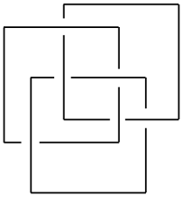
Refer to caption
Figure 23: Borromean Rings
Refer to caption
Figure 24: A Teleportation Scenario
Refer to caption
Figure 25: Teleportation Tensors
Refer to caption
Figure 26: Augmented Space
Refer to caption
Figure 27: Entanglement Swap

8.2 Space, Time, Quantum Networks and Entanglement

Here is a summary for understanding quantum teleportation. Take

|δ⟩=12​(|01⟩+|10⟩)ket𝛿12ket01ket10|\delta\rangle=\frac{1}{\sqrt{2}}(|01\rangle+|10\rangle)

as a representative entangled state. Regard |δ⟩ket𝛿|\delta\rangle as representing the state of two particles that we shall call L𝐿L (left) and R𝑅R (right) corresponding to δ𝛿\delta’s right and left tensor factors. Measuring |δ⟩ket𝛿|\delta\rangle results either in |01⟩ket01|01\rangle or |10⟩.ket10|10\rangle. If an observer measures the left particle, and sees 00 then an observer who will measure the right particle must see 111 and vice versa. Nowhere in the quantum state |δ⟩ket𝛿|\delta\rangle is there any information about the distance between the particles L𝐿L and R𝑅R or any information about the relative times for measurements to occur at the locales for these particles.

Note that the entangled state |δ⟩ket𝛿|\delta\rangle is in the tensor product VβŠ—Vtensor-product𝑉𝑉V\otimes V where V𝑉V is a qubit space spanned by |0⟩ket0|0\rangle and |1⟩.ket1|1\rangle. A general element in VβŠ—Vtensor-product𝑉𝑉V\otimes V has the form

|A⟩=a00​|00⟩+a01​|01⟩+a10​|10⟩+a11​|11⟩,ket𝐴subscriptπ‘Ž00ket00subscriptπ‘Ž01ket01subscriptπ‘Ž10ket10subscriptπ‘Ž11ket11|A\rangle=a_{00}|00\rangle+a_{01}|01\rangle+a_{10}|10\rangle+a_{11}|11\rangle,

and can presented as a 2Γ—2222\times 2 matrix

A=[a00a01a10a11].𝐴delimited-[]subscriptπ‘Ž00subscriptπ‘Ž01subscriptπ‘Ž10subscriptπ‘Ž11A=\left[\begin{array}[]{cc}a_{00}&a_{01}\\ a_{10}&a_{11}\end{array}\right].

Thus the matrix for |δ⟩ket𝛿|\delta\rangle is the identity matrix

I=[1001].𝐼delimited-[]1001I=\left[\begin{array}[]{cc}1&0\\ 0&1\end{array}\right].

By the same token, a successful measurement on two tensor lines can be represented in the dual basis spanned by elementary bras as

⟨M|=m00β€‹βŸ¨00|+m01β€‹βŸ¨01|+m10β€‹βŸ¨10|+m11β€‹βŸ¨11|,bra𝑀subscriptπ‘š00bra00subscriptπ‘š01bra01subscriptπ‘š10bra10subscriptπ‘š11bra11\langle M|=m_{00}\langle 00|+m_{01}\langle 01|+m_{10}\langle 10|+m_{11}\langle 11|,

with corresponding matrix

M=[m00m01m10m11].𝑀delimited-[]subscriptπ‘š00subscriptπ‘š01subscriptπ‘š10subscriptπ‘š11M=\left[\begin{array}[]{cc}m_{00}&m_{01}\\ m_{10}&m_{11}\end{array}\right].

Now consider FigureΒ 24 where we have indicated an initial qubit state |Ο•βŸ©ketitalic-Ο•|\phi\rangle tensored with the entangled state |δ⟩.ket𝛿|\delta\rangle. A sucessful measurement has been made on the first two tensor lines. We assert that the state on the final tensor line is given by M​|Ο•βŸ©π‘€ketitalic-Ο•M|\phi\rangle where this denotes the action of the matrix M𝑀M of the measurement ⟨M|bra𝑀\langle M| on the vector |Ο•βŸ©.ketitalic-Ο•|\phi\rangle. The reader will find the details of this calcluation in tele . This means that if Alice is at the site of the left particle and performs the measurement ⟨M|,bra𝑀\langle M|, then she knows that Bob (at the site of the right particle) will have the quantum state M​|Ο•βŸ©.𝑀ketitalic-Ο•M|\phi\rangle. If the matrix M𝑀M is invertible and unitary, Alice can phone Bob and tell him to apply Mβˆ’1superscript𝑀1M^{-1} to the state that he has. The result will be that Bob will then have a perfect copy of the original state |Ο•βŸ©.ketitalic-Ο•|\phi\rangle. This is the key to teleportation. Specific teleportation protocols use an orthonormal measurement basis (for example the so-called Bell basis) such that all the matrices of the basis elements are unitary. Then this teleportation protocal can be applied whenever Alice measures, at her end, the two left tensor lines. It is as if the wiggle in the line in FigureΒ 24 is pulled staight and the new straightened line represents the transformation M.𝑀M. There is a geometry in the tensor diagrams for the teleportation procedure. It is this geometry that we wish to pursue to understand the geometry and topology of entanglement.

In FigureΒ 25 we illustrate the general case for a single qubit teleportation. The entangled state now has matrix E,𝐸E, not neccessarily the identity, an the measurement has matrix M.𝑀M. We then see from the figure that |Οˆβ€²βŸ©=E​M​|ψ⟩.ketsuperscriptπœ“β€²πΈπ‘€ketπœ“|\psi^{\prime}\rangle=EM|\psi\rangle. The matrix E𝐸E of an entangled state is neccessarily invertible, and so when E𝐸E and M𝑀M are unitary, our previous description of the teleportation procedure goes over mutatis mutandis. Using indices, the description of the state transformation is given by the equation

(Οˆβ€²)k=ψi​Mi​j​Ej​k.superscriptsuperscriptπœ“β€²π‘˜superscriptπœ“π‘–subscript𝑀𝑖𝑗superscriptπΈπ‘—π‘˜(\psi^{\prime})^{k}=\psi^{i}M_{ij}E^{jk}.

The important point to note about this index version of the equation is that it is an exact translation of the structure of the tensor network given on the right part of the figure. This tensor network is the detailed expression of the tensor diagram on the left part of FigureΒ 25. This transformation from (ψi)superscriptπœ“π‘–(\psi^{i}) to (Οˆβ€²)k=ψi​Mi​j​Ej​ksuperscriptsuperscriptπœ“β€²π‘˜superscriptπœ“π‘–subscript𝑀𝑖𝑗superscriptπΈπ‘—π‘˜(\psi^{\prime})^{k}=\psi^{i}M_{ij}E^{jk} can be described by following the connectivity of the tensor network from Alice’s locale to Bob’s locale. The successful measurement ⟨M|bra𝑀\langle M| completes the connection and transforms the quantum information at |ψ⟩ketπœ“|\psi\rangle, located with Alice to |Οˆβ€²βŸ©=E​M​|ψ⟩,ketsuperscriptπœ“β€²πΈπ‘€ketπœ“|\psi^{\prime}\rangle=EM|\psi\rangle, located with Bob. It is a transfer of quantum information, a transfer of quantum states. To obtain observed information transfer one would need to control both measurement at Alice’s end and corresponding measurement at Bob’s end. Nevertheless, the tensor network for the entanglement can be viewed as a way to augment the simple space between Alice and Bob. This extra connectivity between Alice and Bob resides in the entangled state |E⟩ket𝐸|E\rangle that connects them.

We formalize the idea that the tensor network for quantum entanglement can augment the original physical space to create a new connectivity. Let S𝑆S be the given background space for the physical locations of particles. For each entangled state |E⟩ket𝐸|E\rangle with corresponding particles (approximately) located at points L𝐿L and R𝑅R in the space S𝑆S associate a new point E𝐸E and a new open neighborhood {L,E,R}𝐿𝐸𝑅\{L,E,R\} for this new point E.𝐸E. Let Sβ€²superscript𝑆′S^{\prime} be the new space with topology generated by these new neighborhoods of points corresponding to the entangled states. We call Sβ€²superscript𝑆′S^{\prime} the quantum tensor space associated with S𝑆S and its quantum network. See FigureΒ 26 for an illustration of this concept.

To construct the quantum tensor space, we introduce a least topological structure that can produce the special connection between L𝐿L annd R.𝑅R. Note that the new space has non-Hausdorff points for each entangled state. The neighborhood {L,E,R}𝐿𝐸𝑅\{L,E,R\} is a combnatorial topological analogue of an Einstein-Rosen bridge connecting L𝐿L and R.𝑅R. The analogy is important. Note that an observer in the space Sβ€²,superscript𝑆′S^{\prime}, cannot move continously from L𝐿L to E𝐸E without invoking an open neighborhood of E𝐸E and the least such neighborhood contains R.𝑅R. Letting Alice be the observer at L𝐿L and Bob the observer at R,𝑅R, we can say that Alice and Bob can meet together at the connecting point E𝐸E in the analogue black hole. The point E𝐸E is the analogue of the event horizon of an Einstein-Rosen bridge between L𝐿L and R.𝑅R. We will explore the analogies between connectivity in the the quantum tensor spaces and connectivity via Einstein-Rosen bridges in a later paper. It is possible that for larger networks and states with many particles these precursors to Einstein-Rosen Bridges will approximate the bridges in the continuum spacetime. For our purposes, we introduce this formalism to show how it is possible to weld a combinatorial quantum tensor network to a given background space.

FigureΒ 27 illustrates the procedure known as entanglement swapping. Locations A𝐴A and B𝐡B are connected by a entangled state |E⟩ket𝐸|E\rangle and locations B𝐡B and C𝐢C are connected by an entangled state |Eβ€²βŸ©.ketsuperscript𝐸′|E^{\prime}\rangle. By performing a measurement ⟨M|bra𝑀\langle M| at B𝐡B we connect the two entangled states and make a new entangled state that connects A𝐴A with C.𝐢C. In the process, the entanglement connection with B𝐡B is lost. This example shows how the topology of the quantum tensor space will change under the act of measurement. Just as the quantum network undergoes graphical cut and rejoin operations under measurement, the corresponding quantum space, made by the prescription above, will change its connectivity properties. The actions on our simple spaces are easy to understand. In the case of the E​R=E​P​R𝐸𝑅𝐸𝑃𝑅ER=EPR hypothesis it will be very interesting to see what is the meaning of a procedure such as entanglement swapping.

The purpose of this section of the paper has been to show how topological connectivity in the form of knots and in the form of spatially realized quantum networks can be used to make new points of view about quantum entanglement. These points of view shed new light on both the Aravind hypothesis and the Susskind E​R=E​P​R𝐸𝑅𝐸𝑃𝑅ER=EPR hypothesis. In our opinion the Susskind hypothesis is the deeper of the two and most likely to lead to new physics. Nevertheless, the connections between knot theory and the structure of quantum information are very strong and deserve further investigation.

9 Summary

We have shown that entanglement is a necessary condition for forming invariants from R𝑅R matrices from state summation models in the oriented case, while the arguments used by amsshort do not generalize to the unoriented case for state summation models. We must highlight the fact that this appears to be the first time that the two methods (combinatorial and enhanced Yang-Baxter operators) have been shown to differ. We also have found that there is a potential relationship between virtual knots and quantum entanglement that could elucidate more about the relationship between topology and quantum entanglement. However, there exist quantum algorithms for forming topological invariants of knots that rely on no entanglement at all, as in the quantum algorithm described here for computing the Jones polynomial on three-strand braids, which depends only on a single qubit. In conclusion, by studying the boundary between topological and quantum entanglement we can construct a correspondence between topological invariants and entangling R𝑅R matrices that may have a significant impact on the study of quantum computing. In the final section of the paper we have discussed relations between the ideas of this paper and the entanglement hypotheses of Aravind and the ER = EPR hypothesis of Susskind and his collaborators. In the light of the latter hypothesis we have shown how to augment a space to a new space that contains a topological version of the tensor networks describing its quantum structure.

10 Acknowledgments

Eshan Mehrotra takes pleasure in thanking his teachers, mentors, and parents. We would also like to thank Dr. Vandana Chinwalla and Dr. Robyn Fischer for their part in facilitating the Student Inquiry and Research program at the Illinois Math and Science Academy. This work could not have been possible without the environment of free inquiry they labored to foster. It gives Louis Kauffman great pleasure to thank Stathis Antoniou for stimulating conversations in the course of this research. Kauffman’s work was supported by the Laboratory of Topology and Dynamics, Novosibirsk State University (contract no. 14.Y26.31.0025 with the Ministry of Education and Science of the Russian Federation).

11 APPENDIX

Recall that w​(K)𝑀𝐾w(K) is the writhe of an oriented diagram K𝐾K and that S​C​(K)𝑆𝐢𝐾SC(K) denotes the number of Seifert circuits obtained from the diagram K𝐾K by smoothing all crossings in an oriented manner, and c​r​(K)π‘π‘ŸπΎcr(K) is the number of crossings in the diagram K.𝐾K. Furthermore, P𝑃P and N𝑁N denote the number of positive and negative crossings of K.𝐾K.

We shall prove the following

Lemma. For an oriented link diagram K,𝐾K,

S​C​(K)βˆ’w​(K)βˆ’1≑0(mod2).𝑆𝐢𝐾𝑀𝐾1annotated0pmod2SC(K)-w(K)-1\equiv 0\pmod{2}.

Proof The above equation implies that

S​C​(K)≑w​(K)+1(mod2).𝑆𝐢𝐾annotated𝑀𝐾1pmod2SC(K)\equiv w(K)+1\pmod{2}.

Note that the parity of the writhe of a knot and its crossing number are the same, as

w​(K)=Pβˆ’N≑P+N=c​r​(K)(mod2).𝑀𝐾𝑃𝑁𝑃𝑁annotatedπ‘π‘ŸπΎpmod2w(K)=P-N\equiv P+N=cr(K)\pmod{2}.

Thus, we wish to prove that S​C​(K)≑c​r​(K)+1.π‘†πΆπΎπ‘π‘ŸπΎ1SC(K)\equiv cr(K)+1. From now on, we write S​C𝑆𝐢SC for S​C​(K).𝑆𝐢𝐾SC(K).

Consider a knot diagram where the crossings have been replaced with flat nodes. Note that by Euler’s theorem we have that

v+2=R,𝑣2𝑅v+2=R,

where R𝑅R is the number of regions in the diagram and v𝑣v is the number of nodes (c​r​(K)=vπ‘π‘ŸπΎπ‘£cr(K)=v). This theorem implies that

v≑R(mod2).𝑣annotated𝑅pmod2v\equiv R\pmod{2}.

It follows that

S​C≑R+1(mod2).𝑆𝐢annotated𝑅1pmod2SC\equiv R+1\pmod{2}.

For the unknot, R=2𝑅2R=2 and S​C=1𝑆𝐢1SC=1, as shown below.


R=2𝑅2\textstyle{R=2}S​C=1𝑆𝐢1\textstyle{SC=1}

Imagine that each of the following diagrams is a subsection of a much larger diagram. Take the oriented loop,

Suppose that in this diagram we had that S​C≑R+1(mod2)𝑆𝐢annotated𝑅1pmod2SC\equiv R+1\pmod{2}. After we apply our smoothing we get the following diagram.

Note that this diagram has S​C+1𝑆𝐢1SC+1 Seifert circles and R+2𝑅2R+2 regions, so

S​C+1≑(R+1)+1(mod2)𝑆𝐢1annotated𝑅11pmod2SC+1\equiv(R+1)+1\pmod{2}

.

We now assign the following diagram the value of R𝑅R and S​C𝑆𝐢SC. We want to show that the fact that Rβˆ’S​C≑1(mod2)𝑅𝑆𝐢annotated1pmod2R-SC\equiv 1\pmod{2} is true does not change under regular isotopy.

R𝑅\textstyle{R}S​C𝑆𝐢\textstyle{SC}

The next diagram represents the oriented Reidemeister II move with the orientation of each strand pointing in the same direction. It has been given values Rβ€²superscript𝑅′R^{\prime} and S​C′𝑆superscript𝐢′SC^{\prime}. Note that Rβ€²=R+2superscript𝑅′𝑅2R^{\prime}=R+2 and S​Cβ€²=S​C𝑆superscript𝐢′𝑆𝐢SC^{\prime}=SC in this diagram. Therefore, Rβ€²βˆ’S​Cβ€²=Rβˆ’S​C+2superscript𝑅′𝑆superscript𝐢′𝑅𝑆𝐢2R^{\prime}-SC^{\prime}=R-SC+2, so Rβ€²βˆ’S​C′≑1(mod2)superscript𝑅′𝑆superscript𝐢′annotated1pmod2R^{\prime}-SC^{\prime}\equiv 1\pmod{2}.

Rβ€²superscript𝑅′\textstyle{R^{\prime}}S​C′𝑆superscript𝐢′\textstyle{SC^{\prime}}

The next diagram is the oriented Reidemeister II move with the orientations in the opposite direction.

Rβ€²superscript𝑅′\textstyle{R^{\prime}}S​C′𝑆superscript𝐢′\textstyle{SC^{\prime}}

For this diagram, we must show that two separate cases hold true. In the first case we must check that the relation remains the same if the bottom left strand connects to the top left and the top right strand connects to the bottom right (so Rβ€²=3superscript𝑅′3R^{\prime}=3 and S​Cβ€²=2𝑆superscript𝐢′2SC^{\prime}=2). It is easy to see that this case results in Rβ€²=2superscript𝑅′2R^{\prime}=2 and S​Cβ€²=1𝑆superscript𝐢′1SC^{\prime}=1. In the second case, we connect the bottom left strand to the bottom right and the top right strand to the top left (Rβ€²=2superscript𝑅′2R^{\prime}=2 and S​Cβ€²=1𝑆superscript𝐢′1SC^{\prime}=1). This case results in Rβ€²=3superscript𝑅′3R^{\prime}=3 and S​Cβ€²=2𝑆superscript𝐢′2SC^{\prime}=2. In all of these cases we have that

Rβ€²βˆ’S​C′≑1≑Rβˆ’S(mod2).superscript𝑅′𝑆superscript𝐢′1annotated𝑅𝑆pmod2R^{\prime}-SC^{\prime}\equiv 1\equiv R-S\pmod{2}.

We now present the Reidemeister III move. The strands are labeled in the diagram below. There are several cases for this move as shown below.

↔↔\textstyle{\leftrightarrow}22\textstyle{2}55\textstyle{5}44\textstyle{4}11\textstyle{1}66\textstyle{6}33\textstyle{3}

Case 1: Suppose that 1 connects to 2, 3 connects to 4, and 5 connects to 6. We use the notation (12)​(34)​(56)123456(12)(34)(56) to represent the connections. The resulting diagrams for each side of the relation would be

↔↔\textstyle{\leftrightarrow}

In this case, on the left side Rβ€²=3superscript𝑅′3R^{\prime}=3 and S​Cβ€²=2𝑆superscript𝐢′2SC^{\prime}=2 so Rβ€²βˆ’S​C′≑1(mod2)superscript𝑅′𝑆superscript𝐢′annotated1pmod2R^{\prime}-SC^{\prime}\equiv 1\pmod{2}. For the right side, Rβ€²=5superscript𝑅′5R^{\prime}=5 and S​Cβ€²=4𝑆superscript𝐢′4SC^{\prime}=4 so Rβ€²βˆ’S​C′≑1(mod2)superscript𝑅′𝑆superscript𝐢′annotated1pmod2R^{\prime}-SC^{\prime}\equiv 1\pmod{2} too.

Case 2: (12)​(36)​(45)123645(12)(36)(45)

↔↔\textstyle{\leftrightarrow}

In this case, on the left Rβ€²=4superscript𝑅′4R^{\prime}=4 and S​Cβ€²=3𝑆superscript𝐢′3SC^{\prime}=3 and on the right Rβ€²=4superscript𝑅′4R^{\prime}=4 and S​Cβ€²=3𝑆superscript𝐢′3SC^{\prime}=3. Both sides satisfy the relation.

Case 3: (16)​(32)​(45)163245(16)(32)(45)

↔↔\textstyle{\leftrightarrow}

The left side has Rβ€²=5superscript𝑅′5R^{\prime}=5 and S​Cβ€²=4𝑆superscript𝐢′4SC^{\prime}=4 and the right side has Rβ€²=3superscript𝑅′3R^{\prime}=3 and S​Cβ€²=2𝑆superscript𝐢′2SC^{\prime}=2.

Case 4: (14)​(32)​(56)143256(14)(32)(56)

↔↔\textstyle{\leftrightarrow}

The left side has Rβ€²=4superscript𝑅′4R^{\prime}=4 and S​Cβ€²=3𝑆superscript𝐢′3SC^{\prime}=3 and the right side has Rβ€²=4superscript𝑅′4R^{\prime}=4 and S​Cβ€²=3𝑆superscript𝐢′3SC^{\prime}=3

Case 5: (52)​(16)​(34)521634(52)(16)(34)

↔↔\textstyle{\leftrightarrow}

The left side has Rβ€²=4superscript𝑅′4R^{\prime}=4 and S​Cβ€²=3𝑆superscript𝐢′3SC^{\prime}=3 and the right side has Rβ€²=4superscript𝑅′4R^{\prime}=4 and S​Cβ€²=3𝑆superscript𝐢′3SC^{\prime}=3.

Case 6: (54)​(16)​(23)541623(54)(16)(23)

↔↔\textstyle{\leftrightarrow}

The left side of the diagram has Rβ€²=5superscript𝑅′5R^{\prime}=5 and S​Cβ€²=4𝑆superscript𝐢′4SC^{\prime}=4. The right side of the diagram Rβ€²=3superscript𝑅′3R^{\prime}=3 and S​Cβ€²=2𝑆superscript𝐢′2SC^{\prime}=2.

Case 7: (54)​(16)​(23)541623(54)(16)(23)

↔↔\textstyle{\leftrightarrow}

The left side of the diagram has Rβ€²=4superscript𝑅′4R^{\prime}=4 and S​Cβ€²=3𝑆superscript𝐢′3SC^{\prime}=3, while the right side of the diagram has Rβ€²=4superscript𝑅′4R^{\prime}=4 and S​Cβ€²=3𝑆superscript𝐢′3SC^{\prime}=3.

In every case we have shown that the parity of S​C𝑆𝐢SC and w​(K)𝑀𝐾w(K) are different. Therefore, S​Cβˆ’w​(K)βˆ’1𝑆𝐢𝑀𝐾1SC-w(K)-1 is always even. This completes the proof of the Lemma. ∎

References

  • (1) G. Alagic, M. Jarret, and S. Jordan, Yang-Baxter operators need quantum entanglement to distinguish knots, (preprint 2015), arXiv:1507.05979v1 21 July 2015.
  • (2) J. Alexander, A lemma on a system of knotted curves, Proc. Nat. Acad. Sci. USA. 9 (1923), 93-95.
  • (3) P. K. Aravind, Borromean entanglement of the GHZ state. in β€˜Potentiality, Entanglement and Passion-at-a-Distance”, ed. by R. S. Cohen et al, pp. 53-59, Kluwer, 1997.
  • (4) R.J. Baxter. Exactly Solved Models in Statistical Mechanics. Acad. Press (1982).
  • (5) J. Birman, Braids, Links, and Mapping Class Groups, Annals of Mathematics Series Number 82, (1974) Princeton University Press, Princeton, New Jersey.
  • (6) V.F.R. Jones, A polynomial invariant for links via von Neumann algebras, Bull. Amer. Math. Soc. 129 (1985), 103–112.
  • (7) V.F.R.Jones. Hecke algebra representations of braid groups and link polynomials. Ann. of Math. 126 (1987), pp. 335-338.
  • (8) V.F.R.Jones. On knot invariants related to some statistical mechanics models. Pacific J. Math., vol. 137, no. 2 (1989), pp. 311-334.
  • (9) V. F. R. Jones, Braid groups, Hecke algebras and type II1 factors. β€œGeometric methods in operator algebras” (Kyoto, 1983), 242 273, Pitman Res. Notes Math. Ser., 123, Longman Sci. Tech., Harlow, 1986.
  • (10) D. Aharonov, V. F. R. Jones, Z. Landau, A polynomial quantum algorithm for approximating the Jones polynomial. STOC’06: Proceedings of the 38th Annual ACM Symposium on Theory of Computing, 427 436, ACM, New York, 2006. quant-ph/0511096.
  • (11) L. H. Kauffman, β€œFormal Knot Theory”, Princeton University Press (1983).
  • (12) L. H. Kauffman, β€œOn Knots”, Princeton University Press (1987).
  • (13) L. H. Kauffman, State models and the Jones polynomial, Topology 26 (1987) 395-407.
  • (14) L. H. Kauffman, Knot theory and statistical mechanics, International Journal of Modern Physics B 11, Nos. 1, 2 (1997), 39-49.
  • (15) L. H. Kauffman, A self-linking invariant of virtual knots, Fundamenta Mathematicae 184 (2004) 135-158.
  • (16) L. H. Kauffman and S. J. Lomonaco, Quantum entanglement and topological entanglement, New Journal of Physics, 4:73.1-73.18, 2002.
  • (17) L. H. Kauffman and S. J. Lomonaco, q-Deformed Spin Networks, Knot Polynomials and Anyonic Topological Quantum Computation, Journal of Knot Theory and Its Ramifications 16 (2007) 267-332.
  • (18) L. H. Kauffman and S. J. Lomonaco, Braiding operators are universal quantum gates, New Journal of Physics, 6:134.1-134.40, 2004. arXiv:quant-ph/0401090.
  • (19) L. H. Kauffman, Teleportation Topology, quant-ph/0407224, (in the Proceedings of the 2004 Byelorus Conference on Quantum Optics), Opt. Spectrosc. 9, 2005, 227-232.
  • (20) L. H. Kauffman and S. J. Lomonaco, A Three-stranded quantum algorithm for the Jones polynomial, Quantum Information and Quantum Computation V, Proceedings of Spie, April 2007, edited by E.J. Donkor, A.R. Pirich and H.E. Brandt, pp.65730T1-17, Intl Soc. Opt. Eng.
  • (21) L. H. Kauffman and S. J. Lomonaco, The Fibonacci model and the Temperley-Lieb algebra, International Journal of Modern Physics B Vol. 22 No. 29 (2008) 5065-5080.
  • (22) L. H. Kauffman and S. J. Lomonaco Jr., Quantum knots, in Quantum Information and Computation II, Proceedings of Spie, 12 -14 April 2004 (2004), ed. by Donkor Pirich and Brandt, pp. 268-284.
  • (23) S. J. Lomonaco and L. H. Kauffman, Quantum Knots and Mosaics, Journal of Quantum Information Processing, Vol. 7, Nos. 2-3, (2008), pp. 85 - 115. http://arxiv.org/abs/0805.0339
  • (24) S. J. Lomonaco and L. H. Kauffman, Quantum knots and lattices, or a blueprint for quantum systems that do rope tricks. Quantum information science and its contributions to mathematics, 209 276, Proc. Sympos. Appl. Math., 68, Amer. Math. Soc., Providence, RI, 2010.
  • (25) S. J. Lomonaco and L. H. Kauffman, Quantizing braids and other mathematical structures: the general quantization procedure. In Brandt, Donkor, Pirich, editors, Quantum Information and Comnputation IX - Spie Proceedings, April 2011, Vol. 8057, of Proceedings of Spie, pp. 805702-1 to 805702-14, SPIE 2011.
  • (26) L. H. Kauffman and S. J. Lomonaco, Quantizing knots groups and graphs. In Brandt, Donkor, Pirich, editors, Quantum Information and Comnputation IX - Spie Proceedings, April 2011, Vol. 8057, of Proceedings of Spie, pp. 80570T-1 to 80570T-15, SPIE 2011.
  • (27) L. H. Kauffman, Knot diagrammatics, in β€œHandbook of Knot Theory”, Edited by William Menasco and Morwen Thistlethwaite, pp. 233-318, (2005) Elsevier B. V.
  • (28) Maldacena, Juan; Susskind, Leonard (2013). ”Cool horizons for entangled black holes”. Fortsch. Phys. 61: 781 811.
  • (29) K. Reidemeister, Knotentheorie, (first published in 1932, Julius Springer, Berlin) Chelsea Publishing Company, New York (1948)
  • (30) N.Y. Reshetikhin and V. Turaev. Ribbon graphs and their invariants derived from quantum groups. Comm. Math. Phys. 127 (1990). pp. 1-26.
  • (31) N.Y. Reshetikhin and V. Turaev. Invariants of Three Manifolds via link polynomials and quantum groups. Invent. Math. 103, 547-597 (1991).
  • (32) D. Yetter, Markov algebras, ”Braids” (Santa Cruz, CA, 1986), 705 730, Contemp. Math., 78, Amer. Math. Soc., Providence, RI, 1988.