Analysis on $60$ GHz Wireless Communications with Beamwidth-Dependent Misalignment

Abstract

High speed wireless access on 60 GHz spectrum relies on high-gain directional antennas to overcome the severe signal attenuation. However, perfect alignment between transmitting and receiving antenna beams is rare in practice and overheard signals from concurrent transmissions may cause significant interference. In this paper we analyze the impact of antenna beam misalignment on the system performance of 60 GHz wireless access. We quantify the signal power loss caused by beam misalignment and the interference power accumulated from neighboring concurrent transmissions whose signals are leaked either via the main-beam pointing in the similar direction or via side-lobe emission, and derive the probability distribution of the signal to interference plus noise power ratio (SINR). For scenarios where interfering transmitters are distributed uniformly at random, we derive upper and lower bounds on the cumulative distribution function (abbreviated as CDF or c.d.f.) of SINR, which can be easily applied to evaluate system performance. We validate our analytical results by simulations where random nodes are uniformly distributed within a circular hall, and evaluate the sensitivity of average throughput and outage probability against two parameters: the half-power (3 dB) beamwidth to main-lobe beamwidth ratio and the beam misalignment deviation to main-lobe beamwidth ratio. Our results indicate that the derived lower bound performs well when the half-power beamwidth to main-lobe beamwidth ratio or the number of concurrent transmission links is small. When the number of active links is high, it is desirable in antenna design to balance the degradation caused by beam misalignment (wider beam is better) and the interference from concurrent transmission (narrower beam is better).

I Introduction

The proliferation of diverse applications and demands of high speed wireless access [1] drives the rapid development of wireless communication on $60$ GHz band, advocated by many academical and industrial bodies, e.g., IEEE 802.11ad Task Group [2], IEEE 802.15.3 Task Group 3c[3], and Wireless Gigabit Alliance (WiGig). Within the $60$ GHz band, the radios encounter many propagation challenges, such as the severe path loss, weak reflection and diffusion, and high penetration loss [4, 5], and therefore the deployment of high-gain directional antennas (arrays) is required. Besides, high directionality has other benefits in systems with concurrent transmissions: it enables high spatial multiplexing to boost the network capacity within a unit area; it lowers the probability of strong interference among current transmissions.

The benefits of directional antennas and the impact of beam misalignment on the performance of wireless networks have been studied in [6, 7, 8, 9] using simplified beam patterns. In general, a narrower beamwidth corresponds to a higher antenna gain and lower probability of experiencing strong interference from concurrent transmissions, which may contribute to significant improvement in network capacity per unit area [9]. In most of previous study, the radiation pattern of directional antennas is usually modeled in an idealized fashion, e.g., a constant large antenna gain within the narrow main-lobe and zero else where. This idealized radiation pattern, often referred as the “flat-top model”, is widely used [10, 11, 12] for system level performance analysis. However, in practice, the radiation patterns of antennas largely depend on their implementation and are usually more more complex: the main-lobe gain is not constant and the side-lobe radiation is non-zero. As the density of nodes increases, the effect of side-lobe radiation and the gradual reduction of main-lobe gain caused by beam misalignment cannot be ignored any more. The maximum beam-forming gain, which can be achieved only if the main-lobe beams of directional transmitting and receiving antennas are perfectly aligned, is rare due to practical implementation constraints. The origin of beam misalignment can be coarsely divided into two categories: imperfection of existing antenna and beamforming techniques [7, 13, 14], such as the analog beamforming impairments, array perturbations, oscillator locking-range based phase error, and the direction-of-arrival (DoA) estimation errors; mobility of communication terminals [15, 16], which invokes tracking error and system reaction delay. Therefore, it is crucial to study the beam pattern and beam alignment error and quantify their impacts on performance degradation.

In recent years, numerous efforts have been devoted in mimicking practical directional antennas and some plausible models are established, e.g., the piece-wised model [17, 18] and the 3GPP model [19]. The impact of radiation pattern and beam alignment on the performance of directional transmissions has been studied in some recent publications. For instance, in [20, 21], directional antennas considering the side-lobe effect are exploited for mmWave wireless personal area networks (WPAN), and the spatial multiplexing gain, impact of radiation efficiency and fairness are discussed. Besides, the side-lobe effect has been studied using a piecewise linear model in [17]. Other related efforts can be seen in [22, 23, 24].

In this paper, we adopt a close-to-reality antenna radiation pattern established in the 3GPP standard [19], where the non-constant main-lobe gain and the nonzero side-lobe radiation gain are correlated via a total radiated power constraint. We measure the beam misalignment and the half-power ($3$-dB) beamwidth by the ratio between their absolute value and the main-lobe beamwidth, and investigate the effects of radiation pattern and misalignment on performance degradation of $60$ GHz wireless systems. We derive the probability distribution of the signal to interference plus noise power ratio (SINR), where the received signal power degrades owing to the imperfection of beam alignment, and the interference power is accumulated through signals leaked from either the side-lobe radiation or the main-lobe beam of surrounding concurrent links. We also establish upper and lower bounds for the CDF of SINR to facilitate the computation in characterizing the network performance. We evaluate via simulations the average throughput and outage probability of an indoor $60$ GHz wireless communication system and quantify the impact of beam misalignment and beam pattern, and demonstrate the trade-off in beam pattern design to balance the robustness against interference and beam misalignment.

The rest of the paper is organized as follows. We present the system model in Section II and derive the probability distribution of SINR in the presence of random beam misalignment in Section III. In Section IV we derive the bounds for the probability distribution of SINR performance. Performance evaluations are performed in Section V and conclusions are in Section VI.

II System Model

II-A Antenna Model with Beam Misalignment

The 3GPP two-dimension directional antenna pattern [19] is adopted in our study, where the antenna gain $G(\theta)$, with respect to the relative angle $\theta$ to its boresight, is given by

$$G\left(\theta\right)=\begin{dcases}G_{m}\cdot 10^{-\frac{3}{10}\left(\frac{2\theta}{\omega}\right)^{2}},&|\theta|\leq\frac{\theta_{m}}{2},\\ G_{s},&\frac{\theta_{m}}{2}\leq|\theta|\leq\pi,\end{dcases}$$ (1)

where $\omega$ denote the half-power (3 dB) beamwidth, and $\theta_{m}$ is the main-lobe beamwidth. $G_{m}$ and $G_{s}$ represent the maximum main-lobe gain and averaged side-lobe gain, respectively. The total radiated power constraint [20, 9] requires that $\int_{-\pi}^{\pi}G(\theta)d\theta=2\pi$, that is,

$$\int_{0}^{\frac{\theta_{m}}{2}}G_{m}10^{-\frac{3}{10}\left(\frac{2\theta}{\omega}\right)^{2}}d\theta+\int_{\frac{\theta_{m}}{2}}^{\pi}G_{s}d\theta=\pi,$$ (2)

and the continuity of the radiation pattern (1) at the critical value $\theta=\frac{\theta_{m}}{2}$ requires

$$G_{m}=G_{s}\cdot 10^{\frac{3}{10}\left(\frac{\theta_{m}}{\omega}\right)^{2}}.$$ (3)

Combining (2) and (3), we can determine $G_{m}$ and $G_{s}$ analytically, in terms of $\theta_{m}$ and $\omega$, as

$$\begin{dcases}G_{s}=\frac{2\pi}{V\left(\theta_{m},\omega\right)+2\pi-\theta_{m}}\\ G_{m}=\frac{2\pi\cdot 10^{\frac{3}{10}\left(\frac{\theta_{m}}{\omega}\right)^{2}}}{V\left(\theta_{m},\omega\right)+2\pi-\theta_{m}}\end{dcases},$$

where $V\left(\theta_{m},\omega\right)$ is given by

$$V\left(\theta_{m},\omega\right)=\int_{0}^{\theta_{m}}10^{\frac{3}{10}\left(\frac{\theta_{m}^{2}-\theta^{2}}{\omega^{2}}\right)}d\theta.$$

To highlight the main-lobe radiation pattern, we introduce the parameter half-power to main-lobe beamwidth ratio

$$\eta\triangleq\frac{\omega}{\theta_{m}}\in\left(0,1\right)$$ (4)

to quantify the attenuation speed of the main beam gain. $\eta\to 1$ indicates an idealized constant-gain beam and $\eta\to 0$ mimics a fast-attenuating pencil beam.

Throughout the paper we assume that the random misalignment, denoted by ${\varepsilon}$, is bounded within the range of the main-lobe beamwidth $\theta_{m}$, namely, $0\leq|{\varepsilon}|\leq\frac{\theta_{m}}{2}$. This assumption is intuitively based on the fact that beam steering deviation exceeding the main-lobe beamwidth should be treated as alignment failure rather than merely an misalignment. Furthermore, we assume that the misalignment $\varepsilon$ follows a truncated normal distribution with zero mean and variance $\sigma_{\varepsilon}^{2}$, that is,

$$f_{\varepsilon}(x)=\frac{\exp\left(-\frac{x^{2}}{2\sigma_{\varepsilon}^{2}}\right)}{\sigma_{\varepsilon}\sqrt{2\pi}\cdot\mathrm{erf}\left(\frac{\theta_{m}}{2\sqrt{2}\sigma_{\varepsilon}}\right)},\ |x|\leq\frac{\theta_{m}}{2},$$ (5)

where $\mathrm{erf}\left(*\right)$ denotes the error function, and $\sigma_{\varepsilon}\in\left[0,\frac{\theta_{m}}{6}\right]$, i.e., $0\leq 3\sigma_{\varepsilon}\leq\frac{\theta_{m}}{2}$, mimicking the $3\sigma$-rule. The misalignment deviation to main-lobe beamwidth ratio is therefore defined as

$$\rho\triangleq\frac{\sigma_{\varepsilon}}{\theta_{m}}\in\left[0,\frac{1}{6}\right].$$ (6)

II-B Network Setting

Figure 1: Illustration of the two dimensional model with beam misalignment, concurrent transmission interference, and side-lobe signal leakage.

We consider a network that consists of $N$ active communication pairs deployed randomly within an area of interest on a two dimensional plane, where for each communication pair $i\in\{1,2,\ldots,N\}$, the main beam of the transmitter $\mathrm{TX}_{i}$ and the main beam of its intended receiver $\mathrm{RX}_{i}$ are approximately aligned after appropriate channel/DoA estimation, position tracking, and beam steering. To highlight the impact of beam misalignment and to simplify presentation, we assume that all the transmitters and receivers have the same antenna radiation pattern as described in (1), and extension to heterogeneous antenna patterns is straightforward. In Fig. 1 we illustrate a snapshot of the beam misalignment and concurrent transmission interference between two neighboring communication pairs. We denote by $\varepsilon_{i}^{t}$ and $\varepsilon_{i}^{r}$ the beam alignment errors (i.e., the angle between the transmission path and misaligned boresight) of the $i^{\mathrm{th}}$ link at the transmitter and the receiver sides, respectively. The incident angle of interference (with respect to the boresight of the receiver) from $\mathrm{TX}_{j}$ to $\mathrm{RX}_{i}$, $i\neq j$, is denoted by $\varphi_{ji}^{r}$, and the departure angle of interference (w.r.t. the boresight of the transmitter) is represented by $\varphi_{ji}^{t}$.

The desired signal strength can therefore be represented as a function of the beam alignment errors $\varepsilon_{i}^{t}$ and $\varepsilon_{i}^{r}$, and the interference power can be written as a function of the incident angles $\varphi_{ji}^{r}$ and $\varphi_{ji}^{t}$. The SINR at receiver $\mathrm{RX}_{i}$ is written as

$$\gamma_{i}\triangleq\frac{P_{r,i}}{N_{0}+I_{i}}=\frac{P_{t}G\left(\varepsilon_{i}^{t}\right)G\left(\varepsilon_{i}^{r}\right)L\left(d_{i}\right)}{N_{0}+P_{t}\sum\limits_{k\neq i}G\left(\varphi_{ki}^{t}\right)G\left(\varphi_{ki}^{r}\right)L\left(d_{ki}\right)},$$ (7)

where $P_{t}$ is the transmit power, $N_{0}$ is the noise power, and $G(\theta)$ represents the antenna gain with respect to angle $\theta$. $P_{r,i}$ represents the power of the received signal, $I_{i}$ is the aggregate interference power at $\mathrm{RX}_{i}$, $d_{i}$ is the transmission distance from $\mathrm{TX}_{i}$ to $\mathrm{RX}_{i}$, and $d_{ki}$ is the distance from $\mathrm{TX}_{k}$ to $\mathrm{RX}_{i}$, $k\neq i$. $L(d)$ denotes the path loss at distance $d$, which is given by

$$L\left(d\right)=\left(\frac{\lambda}{4\pi}\right)^{2}d^{-\alpha},$$

where $\lambda$ is the carrier wavelength, and $\alpha$ is the path loss attenuation exponent. We assume that $d\geq d_{0}=0.5$ meter to ensure the far field for radio propagation.

III Beam Misalignment and Interference

When the mobility of user terminals is small, the SINR observed during a small period of time relies on the positions of all the active nodes. We describe the positions of an active communication pair in the two dimensional plane by a complex vector $\mathbf{Q}_{i}=\left[Q_{i}^{t},Q_{i}^{r}\right]^{T}\in\mathbb{C}^{2}$, where $Q_{i}^{t}$ and $Q_{i}^{r}$ represent the location information of $\mathrm{TX}_{i}$ and $\mathrm{RX}_{i}$, respectively. Likewise, all the neighboring concurrent transmissions can be captured by vectors $\mathbf{Q}_{j}$, $j\neq i$, based on which the aggregate interference $I_{i}$ can be computed. For the sake of simplicity, we take the node pair $\left(\mathrm{TX}_{1},\mathrm{RX}_{1}\right)$ as the typical object for investigation.

It is worth pointing out that, the received signal power $P_{r,1}$ depends on both $\varepsilon_{1}^{r}$ and $\varepsilon_{1}^{t}$, and the interference power $I_{1}$ depends on $\varepsilon^{r}_{1}$ and $\varepsilon^{t}_{j}$, for $j=2,...,n$. Therefore, $P_{r,1}$ is correlated with $I_{1}$ through $\varepsilon_{1}^{r}$. Given the set of $n$ random location information vectors, namely, $\mathbf{Q}^{(n)}\triangleq\left(\mathbf{Q}_{1},\mathbf{Q}_{2},\ldots,\mathbf{Q}_{n}\right)$ and the beam misalignment $\varepsilon_{1}^{r}$ at $\mathrm{RX}_{1}$, the probability density function (p.d.f.) of the SINR $\gamma_{1}$ can be expressed as

$$\begin{split}f_{\gamma_{1}}\left(x\right)=\idotsint&f_{\gamma_{1}|\mathbf{Q}^{(n)},\varepsilon_{1}^{r}}\left(x|\mathbf{q}^{(n)},e\right)\\ &f_{\mathbf{Q}^{(n)},\varepsilon_{1}^{r}}\left(\mathbf{q}^{(n)},e\right)d\mathbf{q}_{1}\dots d\mathbf{q}_{n}de,\end{split}$$ (8)

where $f_{\gamma_{1}|\mathbf{Q}^{(n)},\varepsilon_{1}^{r}}\left(x|\mathbf{q}^{(n)},e\right)$ is the conditional p.d.f. of $\gamma_{1}$ given $\left(\mathbf{Q}^{(n)},\varepsilon_{1}^{r}\right)=\left(\mathbf{q}^{(n)},e\right)$, with $\mathbf{q}^{(n)}\triangleq\left(\mathbf{q}_{1},\mathbf{q}_{2},\ldots,\mathbf{q}_{n}\right)$. $f_{\mathbf{Q}^{(n)},\varepsilon_{1}^{r}}\left(\mathbf{q}^{(n)},e\right)$ denotes the joint p.d.f. of $\left(\mathbf{Q}^{(n)},\varepsilon_{1}^{r}\right)$, which can be reduced to (due to the independence of $\mathbf{Q}^{(n)}$ and $\varepsilon_{1}^{r}$)

$$f_{\mathbf{Q}^{(n),\varepsilon_{1}^{r}}}\left(\mathbf{q}^{(n)},e\right)=f_{\mathbf{Q}^{(n)}}\left(\mathbf{q}^{(n)}\right)f_{\varepsilon_{1}^{r}}\left(e\right).$$

Proposition 1.

Let $\mathbf{Q}^{(n)}$ and $\varepsilon_{1}^{r}$ be the set of random location information vectors for $n$ links and the beam misalignment at $\mathrm{RX}_{1}$, respectively, the conditional p.d.f. of SINR $\gamma_{1}$ by (7) given $\mathbf{Q}^{(n)}=\mathbf{q}^{(n)}$ and $\varepsilon_{1}^{r}=e$ is obtained as

$$f_{\gamma_{1}|\mathbf{Q}^{(n)},\varepsilon_{1}^{r}}\left(x|\mathbf{q}^{(n)},e\right)=$$ (9)

$$\int_{N_{0}}^{\infty}yf_{P_{r,1}|\mathbf{Q}_{1},\varepsilon_{1}^{r}}\left(xy|\mathbf{q}_{1},e\right)f_{I_{1}|\mathbf{Q}^{(n)},\varepsilon_{1}^{r}}\left(y-N_{0}|\mathbf{q}^{(n)},e\right)dy,$$

where $f_{P_{r,1}|\mathbf{Q}_{1},\varepsilon_{1}^{r}}\left(*|\mathbf{q}_{1},e\right)$ and $f_{I_{1}|\mathbf{Q}^{(n)},\varepsilon_{1}^{r}}\left(*|\mathbf{q}^{(n)},e\right)$ denote the conditional p.d.f. of $P_{r,1}$ and $I_{1}$, respectively.

Proof:

Given two independent positive random variables $Y$ and $W$ with p.d.f. $f_{Y}(y)$ and $f_{W}(w)$, respectively, by applying the p.d.f. computation for the product of two random variables (see Appendix), it is straightforward to derive the p.d.f. of

$$X\triangleq\frac{Y}{c+W}=Y\cdot\left(c+W\right)^{-1},$$

where $c$ is a positive constant. Note that $P_{r,1}$ and $I_{1}$ are conditionally independent given $\mathbf{Q}^{(n)}=\mathbf{q}^{(n)}$ and $\varepsilon_{1}^{r}=e$, we have

$$\begin{split}f_{\gamma_{1}|\mathbf{Q}^{(n)},\varepsilon_{1}^{r}}\left(x|\mathbf{q}^{(n)},e\right)=&\int_{N_{0}}^{\infty}yf_{P_{r,1}|\mathbf{Q}^{(n)},\varepsilon_{1}^{r}}\left(xy|\mathbf{q}^{(n)},e\right)\\ &\cdot f_{I_{1}|\mathbf{Q}^{(n)},\varepsilon_{1}^{r}}\left(y-N_{0}|\mathbf{q}^{(n)},e\right)dy.\end{split}$$

Since $P_{r,1}$ depends on $\mathbf{Q}^{(n)}=\mathbf{q}^{(n)}$ only through $\mathbf{Q}_{1}=\mathbf{q}_{1}$, the p.d.f. of SINR $\gamma_{1}$ can be obtained as (9). ∎

III-A Distribution of Signal Power with Beam Misalignment

Let $P_{t}$ denote the transmit signal power and assume that the transmit beam gain $g_{\varepsilon_{1}^{t}}=G\left(\varepsilon_{1}^{t}\right)$ is a random variable with associated p.d.f. $f_{g}\left(x\right)$, $x\in\left[G_{s},G_{m}\right]$. The received signal power $P_{r,1}$ given $\mathbf{Q}_{1}=\mathbf{q}_{1}\triangleq\left[q_{1}^{t},q_{1}^{r}\right]^{T}\in\mathbb{C}^{2}$ and $\varepsilon_{1}^{r}=e$ can be reformulated as

$$\begin{split}P_{r,1}\big{|}_{\mathbf{Q}_{1}=\mathbf{q}_{1},\varepsilon_{1}^{r}=e}=&P_{t}L\left(d_{11}\right)G\left(e\right)\cdot g_{\varepsilon_{1}^{t}},\end{split}$$ (10)

where $d_{11}{\triangleq}|q_{1}^{r}{-}q_{1}^{t}|$ represents the length of the link. The conditional p.d.f. $f_{P_{r,1}|\mathbf{Q}_{1},\varepsilon_{1}^{r}}\left(x|\mathbf{q}_{1},e\right)$ can therefore be determined by the p.d.f. of $g_{\varepsilon_{1}^{t}}$ as shown below.

Proposition 2.

Let $f_{\varepsilon_{1}^{t}}\left(y\right)$, $|y|{\leq}\theta_{m}/2$ be the p.d.f. of beam misalignment $\varepsilon_{1}^{t}$, the conditional p.d.f. $f_{P_{r,1}|\mathbf{Q}_{1},\varepsilon_{1}^{r}}\left(x|\mathbf{q}_{1},e\right)$ given $\mathbf{Q}_{1}{=}\mathbf{q}_{1}$ and $\varepsilon_{1}^{r}{=}e$ is written as

$$\begin{split}&f_{P_{r,1}|\mathbf{Q}_{1},\varepsilon_{1}^{r}}\left(x|\mathbf{q}_{1},e\right)=\frac{1}{P_{t}L\left(d_{11}\right)g_{e}}f_{g_{\varepsilon_{1}^{t}}}\left(\frac{x}{P_{t}L\left(d_{11}\right)g_{e}}\right),\end{split}$$

where $g_{e}{=}G\left(e\right)$ as described by the radiation pattern (1) and the p.d.f. $f_{g_{\varepsilon_{1}^{t}}}\left(x\right)$ for $\ x\in\left[G_{s},G_{m}\right]$ can be written as

$$f_{g_{\varepsilon_{1}^{t}}}(x)=\frac{\omega f_{\varepsilon_{1}^{t}}\left(\omega\sqrt{\frac{5}{6}\log_{10}\left(\frac{G_{m}}{x}\right)}\right)}{\ln(10)x\sqrt{\frac{6}{5}\log_{10}\left(\frac{G_{m}}{x}\right)}}.$$ (11)

Proof:

Since $0\leq e\leq\theta_{m}/2$, for $g_{e}=G\left(e\right)$ we can derive from (1) that

$$e=\frac{\omega}{2}\sqrt{\frac{10}{3}\log_{10}\left(\frac{G_{m}}{g_{e}}\right)}.$$

Note that the function $g_{e}=G(e)$ is differentiable within the interval $0\leq e<\theta_{m}/2$, we have

$$G^{\prime}(e)=-\frac{12\ln\left(10\right)}{5\omega^{2}}eg_{e}=-\frac{2\ln\left(10\right)}{\omega}g_{e}\sqrt{\frac{6}{5}\log_{10}\left(\frac{G_{m}}{g_{e}}\right)},$$

and the p.d.f. of $g_{e}$ can be straightforwardly derived from the p.d.f. $f_{\epsilon}(e)$ given in (5), as shown in (11). We can now apply (11) to (10) to conclude the proof. ∎

III-B Distribution of Interference Power

Let $I_{1}=\sum_{j=2}^{n}I_{j1}$ be the sum interference power where $I_{j1}$ is the interference power from the $j^{\mathrm{th}}$ concurrent transmission to $\mathrm{RX}_{1}$. In Lemma 1, we show that $I_{j1}$, $j=2,3,\ldots,n$ are conditional independent given $\mathbf{Q}^{(n)}=\mathbf{q}^{(n)}$ and $\varepsilon_{1}^{r}=e$.

Lemma 1.

Let $I_{j1}$, $j=2,3,\ldots,n$, denote the interference power to $\mathrm{RX}_{1}$ from $\mathrm{TX}_{j}$, the conditional joint p.d.f. $f_{I_{21},\ldots,I_{n1}|\mathbf{Q}^{(n)},\varepsilon_{1}^{r}}\left(x_{2},\ldots,x_{n}|\mathbf{q}^{(n)},e\right)$ can be written as

$$\begin{split}&f_{I_{21},\ldots,I_{n1}|\mathbf{Q}^{(n)},\varepsilon_{1}^{r}}\left(x_{2},\ldots,x_{n}|\mathbf{q}^{(n)},e\right)\\ =&\prod\limits_{j=2}^{n}f_{I_{j1}|\mathbf{Q}_{1},\mathbf{Q}_{j},\varepsilon_{1}^{r}}\left(x_{j}|\mathbf{q}_{1},\mathbf{q}_{j},e\right),\end{split}$$

where $f_{I_{j1}|\mathbf{Q}_{1},\mathbf{Q}_{j},\varepsilon_{1}^{r}}\left(*|\mathbf{q}_{1},\mathbf{q}_{j},e\right)$ , $j=2,\ldots,n$, is the conditional p.d.f. of $I_{j1}$ given both $\mathbf{Q}_{1}=\mathbf{q}_{1}$, $\mathbf{Q}_{j}=\mathbf{q}_{j}$ and $\varepsilon_{1}^{r}=e$.

Proof:

Given $\mathbf{Q}^{(n)}=\mathbf{q}^{(n)}$ and $\varepsilon_{1}^{r}=e$, it is easy to obtain that

$$\begin{split}&f_{I_{21},\ldots,I_{n1}|\mathbf{Q}^{(n)},\varepsilon_{1}^{r}}\left(x_{2},\ldots,x_{n}|\mathbf{q}^{(n)},e\right)\\ \overset{(a)}{=}&\prod\limits_{j=2}^{n}f_{I_{j1}|I_{(j+1)1},\ldots,I_{n1},\mathbf{Q}^{(n)},\varepsilon_{1}^{r}}\left(x_{j}|x_{(j+1)},\ldots,x_{n},\mathbf{q}^{(n)},e\right)\\ \overset{(b)}{=}&\prod\limits_{j=2}^{n}f_{I_{j1}|\mathbf{Q}^{(n)},\varepsilon_{1}^{r}}\left(x_{j}|\mathbf{q}^{(n)},e\right)\\ \overset{(c)}{=}&\prod\limits_{j=2}^{n}f_{I_{j1}|\mathbf{Q}_{1},\mathbf{Q}_{j},\varepsilon_{1}^{r}}\left(x_{j}|\mathbf{q}_{1},\mathbf{q}_{j},e\right),\end{split}$$

where $(a)$ applies the chain rule of conditional p.d.f. for multivariate random variables, $(b)$ comes from the fact that $I_{j1}--(\mathbf{Q}^{(n)},\varepsilon_{1}^{r})--I_{j^{\prime}1}$ forms a markov chain for all $j^{\prime}\neq j$, $(c)$ is due to the dependence of $I_{j1}$ on $\mathbf{Q}^{(n)}=\mathbf{q}^{(n)}$ only through the the pair $\left(\mathrm{TX}_{j},\mathrm{RX}_{1}\right)$, which reduces the condition $\mathbf{Q}^{(n)}=\mathbf{q}^{(n)}$ to $\mathbf{Q}_{1}=\mathbf{q}_{1}$ and $\mathbf{Q}_{j}=\mathbf{q}_{j}$. ∎

Since the component interference $I_{j1}$ given $\mathbf{Q}^{(n)}{=}\mathbf{q}^{(n)}$ and $\varepsilon_{1}^{r}{=}e$ can be reformulated as

$$I_{j1}\big{|}_{\mathbf{Q}^{(n)}=\mathbf{q}^{(n)},\varepsilon_{1}^{r}=e}=P_{t}L\left(d_{j1}\right)G\left(\varphi_{j1}^{r}\right)\cdot g_{\varphi_{j1}^{t}},$$ (12)

where $d_{j1}\triangleq|q_{1}^{r}-q_{j}^{t}|$ is the distance between $\mathrm{TX}_{j}$ and $\mathrm{RX}_{1}$, and $g_{\varphi_{j1}^{t}}\triangleq G\left(\varphi_{j1}^{t}\right)$ is a function of random variable $\varphi_{j1}^{t}$, we will establish in Lemma 2 the conditional p.d.f. of $\varphi_{j1}^{t}$.

Lemma 2.

Given $\mathbf{Q}^{(n)}=\mathbf{q}^{(n)}$, the departure angle $\varphi_{j1}^{t}\in\left[0,\pi\right]$ of the interfering link $\left(\mathrm{TX}_{j},\mathrm{RX}_{1}\right)$ can be written as

$$\begin{split}\varphi_{j1}^{t}\big{|}_{\mathbf{Q}^{(n)}=\mathbf{q}^{(n)}}\!=\!\begin{dcases}|2\pi-|\hat{\varphi}_{j1}^{t}-\varepsilon_{j}^{t}||,&|\hat{\varphi}_{j1}^{t}-\varepsilon_{j}^{t}|\geq\pi,\\ |\hat{\varphi}_{j1}^{t}-\varepsilon_{j}^{t}|,&\mbox{otherwise},\end{dcases}\end{split}$$ (13)

where $\hat{\varphi}_{j1}^{t}\triangleq\angle\left(\frac{q_{j}^{r}-q_{j}^{t}}{q_{1}^{r}-q_{j}^{t}}\right)\in\left[-\pi,\pi\right)$ represents the signed angle under perfect beam alignment given $\mathbf{Q}^{(n)}=\mathbf{q}^{(n)}$. Its conditional p.d.f. $f_{\varphi_{j1}^{t}|\mathbf{Q}^{(n)}}\left(*|\mathbf{q}^{(n)}\right)$ is given by

$$f_{\varphi_{j1}^{t}|\mathbf{Q}^{(n)}}\left(x|\mathbf{q}^{(n)}\right)=\left(1-F_{z|\mathbf{Q}^{(n)}}\left(2\pi\right)\right)f_{z|\mathbf{Q}^{(n)}}\left(x+2\pi\right)$$

$$+\left(F_{z|\mathbf{Q}^{(n)}}\left(2\pi\right)-F_{z|\mathbf{Q}^{(n)}}\left(\pi\right)\right)f_{z|\mathbf{Q}^{(n)}}\left(2\pi-x\right)$$ (14)

$$+F_{z|\mathbf{Q}^{(n)}}\left(\pi\right)f_{z|\mathbf{Q}^{(n)}}\left(x\right),$$

where $f_{z|\mathbf{Q}^{(n)}}\left(*\right)$ and $F_{z|\mathbf{Q}_{(n)}}\left(*\right)$ denote the conditional p.d.f. and c.d.f., respectively, of $z=|\hat{\varphi}_{j1}^{t}-\varepsilon_{j}^{t}|$, with

$$f_{z|\mathbf{Q}^{(n)}}\left(x\right)=f_{\varepsilon_{j}^{t}}\left(\hat{\varphi}_{j1}^{t}+x\right)+f_{\varepsilon_{j}^{t}}\left(\hat{\varphi}_{j1}^{t}-x\right).$$ (15)

Proof:

In the absence of beam misalignment, the angle $\hat{\varphi}_{j1}^{t}$ that represents the angle-of-departure (AoD) at $\mathrm{TX}_{j}$ is determined by $\mathbf{Q}^{(n)}{=}\mathbf{q}^{(n)}$. The AoD with misalignment, denoted as $\varphi_{j1}^{t}$, is the sum of the deterministic $\hat{\varphi}_{j1}^{t}$ and a stochastic $\varepsilon_{j}^{t}$, as modeled in (13). Setting $z{=}|\hat{\varphi}_{j1}^{t}-\varepsilon_{j}^{t}|$, its conditional c.d.f. $F_{z|\mathbf{Q}^{(n)}}\left(t\right)$ can be expressed as

$$F_{z|\mathbf{Q^{(n)}}}\left(t|\mathbf{q}^{(n)}\right)=\mathbb{P}\left(|\hat{\varphi}_{j1}^{t}-\varepsilon_{j}^{t}|\leq t\right),$$

from which the conditional p.d.f. $f_{z|\mathbf{Q}_{(n)}}\left(t|\mathbf{q}_{(n)}\right)$ can be obtained. Furthermore, we have

$$\begin{split}&F_{\varphi_{j1}^{t}|\mathbf{Q}^{(n)}}\left(y|\mathbf{q}^{(n)}\right)=\mathbb{P}\left(z-2\pi\leq y\right)\mathbb{P}\left(z\geq 2\pi\right)\\ &+\mathbb{P}\left(2\pi-z\leq y\right)\mathbb{P}\left(\pi\leq z<2\pi\right)+\mathbb{P}\left(z\leq y\right)\mathbb{P}\left(z<\pi\right).\end{split}$$

Taking the first derivative of $F_{\varphi_{j1}^{t}|\mathbf{Q}^{(n)}}\left(y|\mathbf{q}^{(n)}\right)$ with respect to $y$ leads to (14).∎

Likewise, the arrival angle $\varphi_{j1}^{r}\in\left[0,\pi\right]$ of the interfering link $\left(\mathrm{TX}_{j},\mathrm{RX}_{1}\right)$ given $\mathbf{Q}^{(n)}{=}\mathbf{q}^{(n)}$ and $\varepsilon_{1}^{r}{=}e$ is written as

$$\varphi_{j1}^{r}\big{|}_{\mathbf{q}^{(n)},e}=\begin{dcases}|2\pi-|\hat{\varphi}_{j1}^{r}-e||,&|\hat{\varphi}_{j1}^{r}-e|\geq\pi,\\ |\hat{\varphi}_{j1}^{r}-e|,&\mbox{otherwise},\end{dcases}$$ (16)

where $\hat{\varphi}_{j1}^{r}\triangleq\angle\left(\frac{q_{1}^{t}-q_{1}^{r}}{q_{j}^{t}-q_{1}^{r}}\right)\in\left[-\pi,\pi\right)$ is the angle corresponding to the perfect beam alignment given $\mathbf{Q}^{(n)}{=}\mathbf{q}^{(n)}$.

Proposition 3.

The p.d.f. of $I_{j1}$ given $\mathbf{Q}_{1},\mathbf{Q}_{j},\varepsilon_{1}^{r}$ is

$$f_{I_{j1}|\mathbf{Q}_{1},\mathbf{Q}_{j},\varepsilon_{1}^{r}}\left(x|\mathbf{q}_{1},\mathbf{q}_{j},e\right)$$ (17)

$$= \frac{1}{P_{t}L\left(d_{j1}\right)g_{\varphi_{j1}^{r}}}f_{g_{\varphi_{j1}^{t}}|\mathbf{Q}_{1},\mathbf{Q}_{j}}\bigg{(}\frac{x}{P_{t}L\left(d_{j1}\right)g_{\varphi_{j1}^{r}}}\big{|}\mathbf{q}_{1},\mathbf{q}_{j}\bigg{)},$$

where, for $x\in\left[G_{s},G_{m}\right]$, we have

$$\begin{split}f_{g_{\varphi_{j1}^{t}}|\mathbf{Q}_{1},\mathbf{Q}_{j}}\left(x|\mathbf{q}^{(n)}\right)=\frac{\omega f_{\varphi_{j1}^{t}|\mathbf{Q}^{(n)}}\left(\omega\sqrt{\frac{5}{6}\log_{10}\left(\frac{G_{m}}{x}\right)}\Big{|}\mathbf{q}^{(n)}\right)}{\ln(10)x\sqrt{\frac{6}{5}\log_{10}\left(\frac{G_{m}}{x}\right)}}.\end{split}$$

Proof:

By (12), (16), and Lemma 2, it is straightforward to obtain the results by applying the similar method as shown in Proposition 2. ∎

We can now derive the conditional p.d.f. of $I_{1}$ as follows.

Proposition 4.

The conditional p.d.f. of the sum interference given $\mathbf{Q}^{(n)}=\mathbf{q}^{(n)}$ and $\varepsilon_{1}^{r}=e$ is given by

$$f_{I_{1}|\mathbf{Q}^{(n)},\varepsilon_{1}^{r}}\left(x|\mathbf{q}^{(n)},e\right)=\bigotimes_{j=2}^{n}f_{I_{j1}|\mathbf{Q}_{1},\mathbf{Q}_{j},\varepsilon_{1}^{r}}\left(x|\mathbf{q}_{1},\mathbf{q}_{j},e\right),$$

where $\bigotimes$ represents the convolution operator.

Proof:

Since $I_{j1}$, $j{=}2,3,\ldots,n$, are conditionally independent given $\mathbf{Q}^{(n)}{=}\mathbf{q}^{(n)}$ and $\varepsilon_{1}^{r}{=}e$, the p.d.f. of the sum of independent random variables equals the convolution of all the individual probability functions. ∎

Finally, the conditional p.d.f. of SINR in Proposition 1 can be obtained by applying Proposition 2 and Proposition 4, which is then used to compute the p.d.f. of SINR using (8).

IV CDF of SINR: Upper Bound and Lower Bound

It is rather involved to directly evaluate the SINR performance based on the equations derived in the Sec. III, partially due to the convolution of p.d.f. in Proposition 4. For scenarios where there are $K$ interfering transmitters distributed uniformly at random around the receiving node $\mathrm{RX}_{1}$, whose location $\mathbf{Q}_{1}=\mathbf{q}_{1}$ and beam misalignment $\varepsilon_{1}^{r}=e$ are given, we derive upper and lower bounds on the c.d.f. of SINR for $\mathrm{RX}_{1}$. According to Lemma 1, we know that, in the presence of the given $\mathbf{Q}_{1}$ and $\varepsilon_{1}^{r}$, the component interference power $I_{j1}$, $j\in\{2,\ldots,K+1\}$, can be treated as independent random variables. Furthermore, $I_{j1}$ are also identically distributed random variables due to the uniform deployments and orientations. Thus, the interference $I_{j1}$ can be viewed as independent and identically distributed (i.i.d.) random variables.

Following Lemma 1 and Proposition 3, we can obtain the conditional probability $f_{I_{j1}|\mathbf{Q}_{1},\varepsilon_{1}^{r}}\left(*|\mathbf{q}_{1},e\right)$ by marginalizing out the variable $\mathbf{Q}_{j}$, which covers the location information of the $j^{\mathrm{th}}$ transmission pair. Since only $Q_{j}^{t}$ is required for the marginalization process, we have

$$f_{I_{j1}|\mathbf{Q}_{1},\varepsilon_{1}^{r}}\left(x|\mathbf{q}_{1},\!e\right)\!=\! \int\!\!f_{I_{j1}|\mathbf{Q}_{1},Q_{j}^{t},\varepsilon_{1}^{r}}\!\left(x|\mathbf{q}_{1},q_{j}^{t},e\right)f_{Q_{j}^{t}}\!\left(q_{j}^{t}\right)dq_{j}^{t}.$$

For notational simplicity, we use $Y$ and $W_{j}$, $2\leq j\leq K+1$, respectively to represent the random variables $P_{r,1}$ and $I_{j1}$ conditional on $\mathbf{Q}_{1}=\mathbf{q}_{1}$ and $\varepsilon_{1}^{r}=e$. We can then rewrite the conditional c.d.f. $\mathbb{P}\left(\gamma_{1}\leq x|\mathbf{q}_{1},e\right)$ as

$$\mathbb{P}\left(\gamma_{1}\leq x|\mathbf{q}_{1},e\right)\triangleq\mathbb{P}\left(\frac{Y}{N_{0}+W_{\sum}}\leq x\right),$$ (18)

where $W_{\sum}\triangleq\sum_{j=2}^{K+1}W_{j}$. Denote the c.d.f. of $Y$ and $W_{\sum}$ by $F_{Y}\left(*\right)$ and $F_{W_{\sum}}\left(*\right)$, respectively. $F_{Y}\left(x\right)$ can be immediately obtained by applying Proposition 2, i.e., $F_{Y}\left(x\right)=\int_{0}^{x}f_{Y}\left(t\right)dt$. For the sum interference $W_{\sum}$ with respect to $K$ ($K\geq 1$) interfering transmitters, from Proposition 4, we know that

$$F_{W_{\sum}}(x)=\int_{0}^{x}f_{W_{\sum}}(t)dt=\int_{0}^{x}\bigotimes_{j=2}^{K+1}f_{W_{j}}(t)dt.$$

Instead of directly computing the convolution of p.d.f., $F_{W_{\sum}}(x)$ can be alternatively obtained by

$$F_{W_{\sum}}(x)= \mathcal{L}^{-1}\left\{\frac{1}{s}\mathbb{E}\left[\exp\left(-sW_{\sum}\right)\right]\right\}\left(x\right)$$

$$= \mathcal{L}^{-1}\left\{\frac{1}{s}\left(\mathcal{L}\left\{f_{W_{j}}\right\}\left(s\right)\right)^{K}\right\}\left(x\right),$$

where $\mathcal{L}$ and $\mathcal{L}^{-1}$ denote Laplace transform and its inversion, respectively, and $s>0$.

We are ready to derive the upper and lower bounds using $F_{Y}(*)$ and $F_{W_{\sum}}(*)$, shown in the following theorem.

Theorem 1.

Let $F_{Y}\left(*\right)$ and $F_{W_{\sum}}\left(*\right)$ denote the c.d.f. of $Y$ and $W_{\sum}$, respectively, then we have

$$\underline{\mathcal{B}}\left(x\right)\leq\mathbb{P}\left(\frac{Y}{N_{0}+W_{\sum}}\leq x\right)\leq\overline{\mathcal{B}}\left(x\right),$$

where $\underline{\mathcal{B}}\left(x\right)$ and $\overline{\mathcal{B}}\left(x\right)$ are respectively given by

$$\underline{\mathcal{B}}\left(x\right)\triangleq\sup_{t\geq 0}\left\{F_{Y}\left((N_{0}+t)x\right)-F_{W_{\sum}}\left(t\right)\right\},$$

and

$$\overline{\mathcal{B}}\left(x\right)\triangleq 1+\inf_{t\geq 0}\left\{F_{Y}\left((N_{0}+t)x\right)-F_{W_{\sum}}\left(t\right)\right\}.$$

Proof:

For the upper bound, for any $t\geq 0$, we have

$$\mathbb{P}\left(\frac{Y}{N_{0}+W_{\sum}}\leq x\right)= \mathbb{P}\left(\frac{Y}{N_{0}+W_{\sum}}\leq x,W_{\sum}\geq t\right)$$

$$+\mathbb{P}\left(\frac{Y}{N_{0}+W_{\sum}}\leq x,W_{\sum}\leq t\right)$$

$$\leq \mathbb{P}\left(W_{\sum}\geq t\right)\!+\!\mathbb{P}\left(Y\leq\left(N_{0}\!+\!t\right)x\right),$$

then, the upper bound $\overline{\mathcal{B}}\left(x\right)$ can be immediately obtained.

For the lower bound, likewise,

$$\mathbb{P}\left(\frac{Y}{N_{0}+W_{\sum}}\geq x\right)= \mathbb{P}\left(\frac{Y}{N_{0}+W_{\sum}}\geq x,W_{\sum}\geq t\right)$$

$$+\mathbb{P}\left(\frac{Y}{N_{0}+W_{\sum}}\geq x,W_{\sum}\leq t\right)$$

$$\leq \mathbb{P}\left(W_{\sum}\leq t\right)\!+\!\mathbb{P}\left(Y\geq\left(N_{0}\!+\!t\right)x\right)$$

holds for any $t\geq 0$, and it subsequently gives

$$\mathbb{P}\left(\frac{Y}{N_{0}+W_{\sum}}\leq x\right)\geq\mathbb{P}\left(Y\leq\left(N_{0}\!+\!t\right)x\right)\!-\!\mathbb{P}\left(W_{\sum}\leq t\right),$$

which concludes the lower bound $\underline{\mathcal{B}}\left(x\right)$. ∎

Note that given $\mathbf{Q}_{1}$ and $\varepsilon_{1}^{r}$, the outage probability can be expressed as the c.d.f. of $\gamma_{1}$, i.e.,

$$p_{1,\mathrm{out}}(R_{\mathrm{th}})\triangleq\mathbb{P}(R_{1}<R_{\mathrm{th}})=F_{\gamma_{1}}\left(2^{R_{\mathrm{th}}/W}-1\right),$$

where $R_{\mathrm{th}}$ denotes the rate threshold. Therefore tight bounds on the c.d.f. are essential in evaluating the performance.

V Performance Evaluation

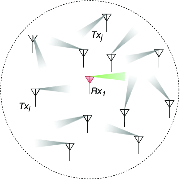
Figure 2: Illustration of multiple interfering transmitters in the area of interest.

We consider a $60$ GHz indoor wireless access network within a circular space of radius $R_{0}=15$ meters, as illustrated in Fig. 2, where there are in total $N=n$ concurrent transmissions. The receiving node in focus, $\mathrm{RX}_{1}$, is located at the center of a circular area and there are totally $K=n-1$ interfering transmitters distributed uniformly at random within the area of interest, randomly oriented in a uniform manner. Results by numerical and Monte-Carlo methods are presented to investigate the accuracy of the bounds, and the sensitivity of outage probability and average throughput against beam patterns and misalignment. To simplify the performance evaluation, all nodes are assumed to be placed on the same horizontal plane. The common system parameters are summarized in Table I and the p.d.f. of link lengths can be found in [25]. Our evaluation consists of the two parts:

1. Numerical results to validate the bounds for the fixed typical receiver $\mathrm{RX}_{1}$, as depicted in Fig. 2.

2. Simulation results to evaluate the average performance of randomly deployed typical receivers.

TABLE I: System Parameters

Parameter	Notation	Value
Wavelength	$\lambda$	$5\times 10^{-3}$ m
Bandwidth	$W$	$500$ MHz
Transmit Power	$P_{t}$	$1$ mW
Main-lobe Beamwidth	$\theta_{m}$	$\left[\frac{\pi}{12},\frac{\pi}{2}\right]$
3dB-Beamwidth Ratio	$\eta$	$\left(0,1\right)$
Misalignment Deviation	$\rho$	$\left[0,\frac{1}{6}\right]$
Noise Power Density	$N_{0}/W$	$-114$ dBm/MHz
Radius of Circular Hall	$R_{0}$	$15$ m
Path Loss Exponent	$\alpha$	$2.45$
Link Numbers	$n$	$\leq 30$

V-A Bounds for Fixed Typical Receiver at The Center

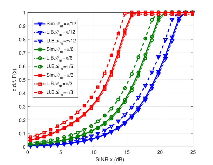
Figure 3: The lower and upper bounds of c.d.f.s for $\gamma_{1}$ and simulated results, with respect to diverse $\theta_{m}$, where $n=11$, $\eta=0.4$, and $\rho=\frac{1}{20}$.

We validate the bounds derived in Theorem 1 for the fixed typical receiver and investigate the impact of the main-lobe beamwidth $\theta_{m}$ and the half-power beamwidth ratio $\eta$ on the c.d.f. of SINR. The lower and upper bounds on the c.d.f. of SINR are illustrated in Fig. 3, where $n=11$, $\eta=0.4$, and $\rho=\frac{1}{20}$. To investigate the impact of $\theta_{m}$ and the associated factor $\eta$, we consider the following three distinct values of beamwidth, i.e., $\theta_{m}=\frac{\pi}{12}$, $\frac{\pi}{6}$, and $\frac{\pi}{3}$, respectively. In general, the derived bounds in Theorem 1 behave well for all groups, which validates the feasibility of applying our upper and lower bounds in analyzing the actual system performance. Note that in all combinations we have considered here, the lower bound outperforms its upper counterpart. Furthermore, considerable performance gain can be achieved by narrowing down the beamwidth. For instance, when $\theta_{m}=\frac{\pi}{3}$ reduces to its half, i.e., $\theta_{m}=\frac{\pi}{6}$, there is roughly $4$ dB gain, and there is another $3$ dB gain when $\theta_{m}$ keeps going down to $\theta_{m}=\frac{\pi}{12}$.

Figure 4: The lower and upper bounds of c.d.f.s for $\gamma_{1}$ and simulated results, with respect to diverse $\eta$, where $n=21$, $\theta_{m}=\frac{\pi}{6}$ and $\rho=\frac{1}{20}$.

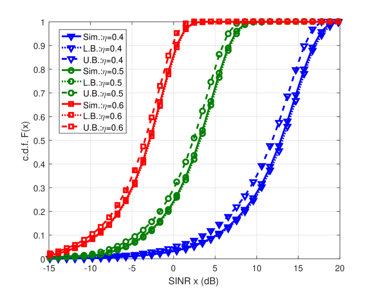
In Fig. 4, we demonstrate the bound performance against the factor $\eta$, where $n=21$, $\theta_{m}=\frac{\pi}{6}$ and $\rho=\frac{1}{20}$. Again, both the upper and lower bounds are very tight. Despite of a narrow beamwidth, i.e., $\theta_{m}=\frac{\pi}{6}$, is employed, there is still huge performance difference for different $\eta$. As shown in the figure, a substantial gain can be achieved by decreasing $\eta$ (i.e., a faster attenuating main-lobe). For instance, the performance gains roughly $6$ dB when decreasing $\eta$ from $0.6$ to $0.5$, while roughly $10$ dB gain can be achieved by $\eta=0.4$. This indicates the great importance of $\eta$ in the antenna design.

The above results show that, both the main-lobe beamwidth and the half-power beamwidth ratio are crucial factors that determine the performance. In what follows, we will consider the scenario where the typical receiver is randomly located.

V-B Simulations for Randomly Located Typical Receiver

In contrast to the aforementioned scenario with fixed $\mathbf{Q}_{1}$ and $\varepsilon_{1}^{r}$, we here focus on the situation where the typical receiver is randomly located, and the misalignment is not given. Besides the outage probability, in this section, the sum throughput and the average throughput are also evaluated.

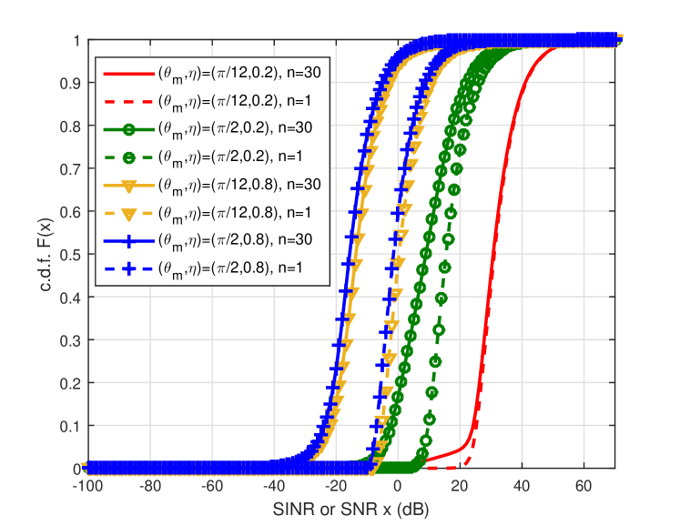
Figure 5: The c.d.f.s of SINR $\gamma_{1}$ with diverse $(\theta_{m},\eta)$ pairs for $n=1$ or $30$, where $\rho=\frac{1}{20}$.

In Fig. 5, we illustrate the c.d.f. of $\gamma_{1}$ with the fixed misalignment derivation to main-lobe beamwidth ratio $\rho{=}\frac{1}{20}$, where the main-lobe beamwidth $\theta_{m}$ is set to be $\frac{\pi}{12}$ or $\frac{\pi}{2}$, and the half-power beamwidth ratio $\eta$ is chosen as $0.2$ or $0.8$. We denote by $F_{{\gamma}_{1}}^{(1)}\left(x\right)$ and $F_{{\gamma}_{1}}^{(30)}\left(x\right)$ the outage probabilities associated with $n=1$ (hence no concurrent transmission interference) and $n=30$, respectively. For $\left(\theta_{m},\eta\right){=}\left(\frac{\pi}{12},0.2\right)$ that corresponds to the scenario where the main-lobe is narrow and the beam attenuates fast, there is only a small gap between $F_{\gamma_{1}}^{(30)}\left(x\right)$ and $F_{\gamma_{1}}^{(1)}\left(x\right)$. This is in line with our intuition that when the receive beam is very narrow and the beam misalignment is small, the degradation caused by concurrent transmission interference is not significant except for users with low signal power. If we then hold $\eta{=}0.2$ (i.e., fast attenuation beam) but increase the main-lobe beamwidth $\theta_{m}$ from $\frac{\pi}{12}$ to $\frac{\pi}{2}$, the gap between $F_{\gamma_{1}}^{(30)}\left(x\right)$ and $F_{\gamma_{1}}^{(1)}\left(x\right)$, with a gap of around $5$dB at $10$-percentile and 1dB at $90$-percentile. Interestingly, if we set $\eta{=}0.8$, i.e., the main-lobe has almost a constant-gain top, the gap between upper and lower bounds remains almost a constant of 8dB from $10$-percentile up to $90$-percentile, and the influence of the main-lobe beamwidth $\theta_{m}$ is very limited: less than 1 dB gap between $\theta_{m}=\frac{\pi}{12}$ and $\theta_{m}=\frac{\pi}{2}$. Therefore, when beam misalignment is small, the main-lobe attenuation speed, quantified by $\eta$, dominates the sensitivity to concurrent transmission interference.

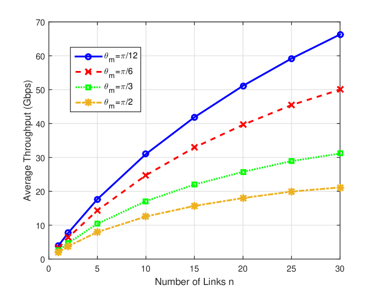
Figure 6: The average sum throughput with varying $n\leq 30$, where $\theta_{m}=\frac{\pi}{12},\frac{\pi}{6},\frac{\pi}{3}$ or $\frac{\pi}{2}$, $\rho{=}\frac{1}{20}$, and $\eta{=}\frac{1}{2.6}$.

In Fig. 6 we plot the average sum throughput as a function of the number of active links $n$ ranging from $1$ to $30$, where the main-lobe beamwidth $\theta_{m}$ is set to $\frac{\pi}{12}$, $\frac{\pi}{6}$, $\frac{\pi}{3}$, and $\frac{\pi}{2}$, respectively, with fixed misalignment derivation to main-lobe beamwidth ratio $\rho{=}\frac{1}{20}$ and half-power beamwidth ratio $\eta{=}\frac{1}{2.6}$, which is adopted from the experiment validation in [26]. As the number of active links increases, the average sum throughput increases much faster for narrow beam $\theta_{m}{=}\frac{\pi}{12}$ compared to wide beam $\theta_{m}{=}\frac{\pi}{2}$, as determined by the slopes of the curves. This is in line with our observations from Fig. 5 where, when the main-lobe attenuates fast, the links with small main-lobe beamwidth are more or less noise/power limited whereas the links with large main-lobe are interference limited.

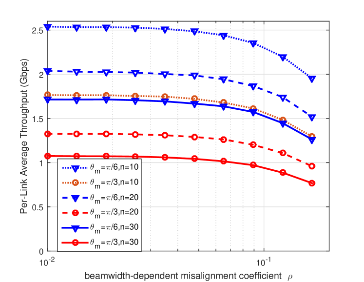
Figure 7: Sensitivity of the per-link average throughput against $\rho$, where $\eta=\frac{1}{2.6}$, $\theta_{m}=\frac{\pi}{6}$ or $\frac{\pi}{3}$, and $n=10,20$ or $30$.

In Fig. 7 we investigate the sensitivity of the per-link average throughput against $\rho$ with a fixed half-power beamwidth ratio $\eta=\frac{1}{2.6}$. We investigate two groups with $\theta_{m}=\frac{\pi}{6}$ and $\frac{\pi}{3}$, respectively, with the number of active links $n=10$, $20$ or $30$. For any given $\rho$, the per-link average throughput will decrease significantly as the main-lobe beamwidth $\theta_{m}$ and/or the number of active links $n$ increases, which clearly attributes to the increase of the concurrent transmission interference. Such per-link performance degradation (gap among different lines) decreases slightly as the misalignment increases. For fixed $n$ and $\theta_{m}$, the per-link average throughput remains stable for $\rho<0.05$ and the degradation grows up to about $30\%$ as $\rho\to\frac{1}{6}$. Regarding the practical significance, on the one hand, it is beneficial to reduce beam misalignment, but the reward is diminishing as $\rho$ becomes smaller. Since a high alignment precision indicates a high overhead/cost in practical implementations, a quantitative evaluation of the performance loss is crucial to seek the proper trade-off between the performance and cost. On the other hand, the performance degradation caused by $\rho$ remains almost the same as the main-lobe beamwidth increases from $\frac{\pi}{6}$ to $\frac{\pi}{2}$, which clearly justifies our effort in quantifying the misalignment via $\rho$.

VI Conclusions

We study the impact of antenna beam misalignment and beam patterns on the system performance of $60$ GHz wireless access. A practical directional antenna model that considering both the main-lobe and side-lobe gains is applied. We introduced two main-lobe beamwidth-dependent parameters, namely, the half-power beamwidth ratio $\eta$ to quantify the main-lobe attenuation speed, and the misalignment deviation ratio $\rho$ to quantify the concentration of beam misalignment. We derived the probability distribution of the SINR, and developed tight upper and lower bounds to facilitate tractable performance analysis. Our numerical results demonstrate the tightness of our derived upper and lower bounds, and reveal that the parameter $\eta$ plays a critical role in enhancing the network performance. Furthermore, we quantified the sensitivity of performance deterioration with respect to beam misalignment and aggregated interferences from neighboring concurrent transmissions. Our results reveal the importance of the two key parameters $\eta$ and $\rho$ in system design to balance the impact of beam misalignment and concurrent transmission interference.

Appendix A Product of Two Random Variables

Without loss of generality, assuming $c$ is a non-zero constant scalar, let $X=cYZ$ be a function of two positive random variables $Y$ and $Z$, with marginal p.d.f.s $f_{Y}(y)$ and $f_{Z}(z)$, accordingly, where $c$. Introducing an auxiliary random variable $v=z$, with $x=cyz$, we can obtain $y=\frac{x}{cv}$ and $z=v$, respectively. Through the function of multivariate random variables [27], we have

$$f_{X,V}(x,v)=\frac{f_{Y,Z}(y,z)}{|\mathcal{J}_{x,v}\left(y,z\right)|},$$

where $\mathcal{J}_{x,v}\left(y,z\right)$ is given by

$$\mathcal{J}_{x,v}\left(y,z\right)=\begin{vmatrix}\frac{\partial x}{\partial y}&\frac{\partial x}{\partial z}\\ \frac{\partial v}{\partial y}&\frac{\partial v}{\partial z}\end{vmatrix}=\begin{vmatrix}cz&cy\\ 0&1\end{vmatrix}=cv,$$

thus we have

$$f_{X,V}(x,v)=\left(|c|v\right)^{-1}f_{Y,Z}\left(\frac{x}{cv},v\right).$$

Finally, the p.d.f. $f_{X}(x)$ can be immediately obtained by the integral over all possible $v$. That is,

$$f_{X}(x)=\int\limits_{v\in\mathcal{S}_{z}}\left(|c|v\right)^{-1}f_{Y,Z}\left(\frac{x}{cv},v\right)dv,$$

where $\mathcal{S}_{z}$ corresponds to the domain of marginal p.d.f. of $Z$, namely, $f_{Z}(z)$.

Particularly, if $Y$ and $Z$ are independent random variables, we further have

$$f_{X}(x)=\int\limits_{v\in\mathcal{S}_{z}}\left(|c|v\right)^{-1}f_{Y}\left(\frac{x}{cv}\right)f_{Z}\left(v\right)dv.$$

References

• [1] Cisco Visual Networking Index: Global Mobile Data Traffic Forecast Update 2014–2019 White Paper. Cisco Systems, Inc. [Online]. Available: http://www.cisco.com/c/en/us/solutions/collateral/service-provider/visual-networking-index-vni/white_paper_c11-520862.pdf
• [2] 802.11ad, Part 11: Wireless LAN Medium Access Control (MAC) and Physical Layer (PHY) Specifications–Amendment 3: Enhancements for Very High Throughput in the 60 GHz Band, IEEE Std., 2012.
• [3] 802.15.3c, Part 15.3: Wireless Medium Access Control (MAC) and Physical Layer (PHY) Specifications for High Rate Wireless Personal Area Networks (WPANs) – Amendment 2: Millimeter-wave-based Alternative Physical Layer Extension, IEEE Std., 2009.
• [4] N. Moraitis and P. Constantinou, “Measurements and characterization of wideband indoor radio channel at 60 GHz,” IEEE Transactions on Wireless Communications, vol. 5, no. 4, pp. 880–889, 2006.
• [5] S. Geng, J. Kivinen, X. Zhao, and P. Vainikainen, “Millimeter-wave propagation channel characterization for short-range wireless communications,” IEEE Transactions on Vehicular Technology, vol. 58, no. 1, pp. 3–13, 2009.
• [6] R. Ramanathan, J. Redi, C. Santivanez, D. Wiggins, and S. Polit, “Ad hoc networking with directional antennas: a complete system solution,” IEEE Journal on Selected Areas in Communications, vol. 23, no. 3, pp. 496–506, 2005.
• [7] J. Yu, Y.-D. Yao, A. F. Molisch, and J. Zhang, “Performance evaluation of CDMA reverse links with imperfect beamforming in a multicell environment using a simplified beamforming model,” IEEE Transactions on Vehicular Technology, vol. 55, no. 3, pp. 1019–1031, 2006.
• [8] B. Epple, “Using a GPS-aided inertial system for coarse-pointing of free-space optical communication terminals,” in SPIE Optics & Photonics.   International Society for Optics and Photonics, 2006, pp. 630 418–630 418.
• [9] J. Wildman, P. Nardelli, M. Latva-aho, S. Weber et al., “On the joint impact of beamwidth and orientation error on throughput in directional wireless Poisson networks,” IEEE Transactions on Wireless Communications, vol. 13, no. 12, pp. 7072–7085, 2014.
• [10] J. E. Wieselthier, G. D. Nguyen, and A. Ephremides, “Energy-limited wireless networking with directional antennas: the case of session-based multicasting,” in IEEE 21st Annual Joint Conference of the IEEE Computer and Communications Societies (INFOCOM 2002), vol. 1.   IEEE, 2002, pp. 190–199.
• [11] I. Kang, R. Poovendran, and R. Ladner, “Power-efficient broadcast routing in adhoc networks using directional antennas: technology dependence and convergence issues,” University of Washington, Washington, USA, Tech. Rep. UWEETR-2003-0015, 2003.
• [12] S. Singh, R. Mudumbai, and U. Madhow, “Interference analysis for highly directional 60-ghz mesh networks: The case for rethinking medium access control,” IEEE/ACM Transactions on Networking, vol. 19, no. 5, pp. 1513–1527, 2011.
• [13] J. Shen and L. W. Pearson, “The phase error and beam-pointing error in coupled oscillator beam-steering arrays,” IEEE Transactions on Antennas and Propagation, vol. 53, no. 1, pp. 386–393, 2005.
• [14] H. Li, Y.-D. Yao, and J. Yu, “Outage probabilities of wireless systems with imperfect beamforming,” IEEE Transactions on Vehicular Technology, vol. 55, no. 5, pp. 1503–1515, 2006.
• [15] A. W. Doff, K. Chandra, and R. V. Prasad, “Sensor Assisted Movement Identification and Prediction for Beamformed 60 GHz Links,” in 12th Annual IEEE Consumer Communications and Networking Conference (CCNC), 2015, pp. 648–653.
• [16] S. Hur, T. Kim, D. J. Love, J. V. Krogmeier, T. Thomas, A. Ghosh et al., “Millimeter wave beamforming for wireless backhaul and access in small cell networks,” IEEE Transactions on Communications, vol. 61, no. 10, pp. 4391–4403, 2013.
• [17] S. Akoum, O. El Ayach, and R. W. Heath, “Coverage and capacity in mmWave cellular systems,” in Conference Record of the Forty Sixth Asilomar Conference on Signals, Systems and Computers (ASILOMAR).   IEEE, 2012, pp. 688–692.
• [18] F. Baccelli and B. Blaszczyszyn, “Stochastic Geometry and Wireless Networks, Volume II-Applications,” 2009.
• [19] UMTS; Spatial channel model for Multiple Input Multiple Output (MIMO) simulations. ETSI 3rd Generation Partnership Project (3GPP). Sophia Antipolis Cedex, France. 3GPP Tech. Rep. 25.996 version 12.0.0 Release 12. [Online]. Available: http://www.etsi.org/deliver/etsi_tr/125900_125999/125996/12.00.00_60/tr_125996v120000p.pdf
• [20] L. X. Cai, L. Cai, X. S. Shen, and J. W. Mark, “REX: a randomized exclusive region based scheduling scheme for mmWave WPANs with directional antenna,” IEEE Transactions on Wireless Communications, vol. 9, no. 1, pp. 113–121, 2010.
• [21] J. Qiao, L. X. Cai, X. Shen, and J. W. Mark, “Enabling multi-hop concurrent transmissions in 60 GHz wireless personal area networks,” IEEE Transactions on Wireless Communications, vol. 10, no. 11, pp. 3824–3833, 2011.
• [22] S. Yi, Y. Pei, and S. Kalyanaraman, “On the capacity improvement of ad hoc wireless networks using directional antennas,” in Proceedings of the 4th ACM international symposium on Mobile ad hoc networking & computing.   ACM, 2003, pp. 108–116.
• [23] J. Wang, L. Kong, and M.-Y. Wu, “Capacity of wireless ad hoc networks using practical directional antennas,” in IEEE Wireless Communications and Networking Conference (WCNC2010).   IEEE, 2010, pp. 1–6.
• [24] G. Zhang, Y. Xu, X. Wang, and M. Guizani, “Capacity of hybrid wireless networks with directional antenna and delay constraint,” IEEE Transactions on Communications, vol. 58, no. 7, pp. 2097–2106, 2010.
• [25] G. Yang, J. Du, and M. Xiao, “Maximum Throughput Path Selection With Random Blockage for Indoor 60 GHz Relay Networks,” IEEE Transactions on Communications, vol. 63, no. 10, pp. 3511–3524, 2015.
• [26] I. Toyoda, T. Seki, K. Iiguse et al., “Reference antenna model with side lobe for TG3c evaluation,” IEEE 802.15.06-0474-00-003c, Tech. Rep., 2006.
• [27] A. Papoulis and S. U. Pillai, Probability, random variables, and stochastic processes.   Tata McGraw-Hill Education, 2002.