The weirdest SDSS galaxies: results from an outlier detection algorithm

Abstract

How can we discover objects we did not know existed within the large datasets that now abound in astronomy? We present an outlier detection algorithm that we developed, based on an unsupervised Random Forest. We test the algorithm on more than two million galaxy spectra from the Sloan Digital Sky Survey and examine the 400 galaxies with the highest outlier score. We find objects which have extreme emission line ratios and abnormally strong absorption lines, objects with unusual continua, including extremely reddened galaxies. We find galaxy-galaxy gravitational lenses, double-peaked emission line galaxies, and close galaxy pairs. We find galaxies with high ionisation lines, galaxies which host supernovae, and galaxies with unusual gas kinematics. Only a fraction of the outliers we find were reported by previous studies that used specific and tailored algorithms to find a single class of unusual objects. Our algorithm is general and detects all of these classes, and many more, regardless of what makes them peculiar. It can be executed on imaging, time-series, and other spectroscopic data, operates well with thousands of features, is not sensitive to missing values, and is easily parallelisable.

1 Introduction

The amount of astronomical data and its complexity grows rapidly, thus introducing astronomy to the era of Big Data science. Ongoing and future large surveys provide astronomers with a wealth of information to be analysed and extracted from rich and complex data types. The Sloan Digital Sky Survey (SDSS) has provided the community with multi-coloured images of approximately one third of the sky, and spectra of more than three million objects (York et al. 2000). The Palomar Transient Factory (PTF; Law et al. 2009) and Pan-STARRS (Kaiser et al. 2010) monitored the variable night sky and studied numerous asteroids, variable stars, supernovae, active galactic nuclei (AGN), and more. Future surveys will increase by orders of magnitude the number of available objects and the information each of these holds. This includes most notably LSST (Ivezic et al. 2008), DESI (Levi et al. 2013), and ZTF (Bellm 2014). These challenge astronomers to move on from the traditional data analysis and visualisation techniques and develop new, Big-Data appropriate, tools (Pesenson, Pesenson & McCollum 2010).

In view of this accelerating growth, astronomers start to develop automated tools in order to detect, characterise, and classify objects based on the immense amount of information they are gathering. Following that, it is necessary to point towards objects which hold the largest amount of new information by developing automated decision making tools that can process large numbers of objects and draw our specific attention. Supervised Machine Learning (ML) algorithms are used to detect predefined objects of interest, and unsupervised learning algorithms to classify objects and find correlations in high dimensional data (Collister & Lahav 2004; Re Fiorentin et al. 2007; Daniel et al. 2011; Morales-Luis et al. 2011; Richards et al. 2012; Sánchez Almeida & Allende Prieto 2013; Fustes et al. 2013; Masci et al. 2014; Baron et al. 2015; Hocking et al. 2015; Miller 2015; Wright et al. 2015; Djorgovski et al. 2016; Lochner et al. 2016; Mackenzie, Pichara & Protopapas 2016; Rubin & Gal-Yam 2016; for additional references and review see Ball & Brunner 2010).

The natural step after classification and the analysis of different clusters is outlier detection and characterisation. Outliers can be objects that were not intended to be included in the original sample, various errors, extreme objects that reside on the tail of well characterised distributions, and completely new objects which offer the opportunity to unveil new physics. To paraphrase Donald Rumsfeld: normal objects are the ‘known knowns’; outliers of kinds discovered before are ‘known unknowns’; but the most interesting, and challenging to find in large datasets, are the ‘unknown unknowns’, objects we did not know we should be looking for. Our goal in this paper is to present such an outlier detection algorithm and its application on the well studied sample of SDSS galaxy spectra, as a first test.

Random Forest (RF) (Breiman et al. 1984; Breiman 2001) is being used extensively in astronomy, though as a supervised learning algorithm. Its main advantages are that it offers a feature importance ranking, and it can be easily parallelisable. Studies train RF to distinguish between different classes of objects based on their features. This is being done by construction of a sample in which objects are already (manually or via a different method) labeled. This sample is the training sample with which the algorithm is trained to distinguish between different classes of objects. These decision rules are then applied to a sample of interest with no labels. RF is used for classification of transients in PTF (Bloom et al. 2012) and in the Dark Energy Survey (Goldstein et al. 2015), and it was recently proposed for gravitational wave searches of black hole binary coalescence (Baker et al. 2015).

Our outlier detection is based on an unsupervised RF, thus we do not have labeled data, and expect the algorithm to learn the data through its features with no additional user-defined input. Our algorithm is based on the work of Shi & Horvath (2006), but with modifications that make it suitable for this task. For other anomaly detection algorithms see Goix (2016, e.g., the work of ). We test the algorithm on one of the most extensively studied samples - the SDSS galaxy spectra. The twelfth data release (DR12) of SDSS includes spectra of more than 2 million galaxies, approximately half of which were released to the public 7 years ago. These galaxies were characterised and classified thoroughly, and unusual objects were found, making it a useful benchmark (see for example: Sánchez Almeida et al. 2010; Andrae, Melchior & Bartelmann 2010; Ascasibar & Sánchez Almeida 2011; Huertas-Company et al. 2011).

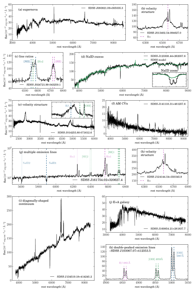
As we show below, we find different kinds of outliers which were found by previous studies, but more importantly, some of the outliers we find are new, even in a sample as thoroughly studied as this one. We show in figure 1 a sample of outlying galaxies that our algorithm detects, some of them are further discussed in later sections. Clearly, we find objects with a wide variety of properties.

We describe the galaxy sample in section 2 and present the outlier detection algorithm in section 3. We then present and discuss the 400 weirdest spectra found by the algorithm in section 4. We conclude with a discussion regarding other potential uses of the algorithm in astronomy in section 5.

Figure 1: A sample of the outliers we find with the outlier detection algorithm, sporting a large variety of unusual features, all found within a single run of the algorithm.

2 Data Set

Our sample consists of all the galaxy spectra from SDSS DR12 (Alam et al. 2015), obtained with both the SDSS and BOSS spectrographs (see Ahn et al. 2012). Although the spectrographs differ in fibre diameter and wavelength coverage we do not divide our sample based on the spectrograph that was used. We have 2 379 168 galaxy spectra in total.

In order to avoid being confused by bad sky subtractions and calibration errors, we use the ‘and_mask’ which marks pixels that are bad throughout all the sub-exposures of a given object. We discard pixels that are marked in ‘and_mask’ and their closest neighbours (one on each side). We completely remove all objects which have more than 700 bad pixels marked in the ‘and_mask’ and remain with 2 355 926 spectra. We further discard the pixels in the wavelength range 5565-5590 Å  in the observers frame due to residual sky emission which occurs in a large number of the objects.

The SDSS spectroscopic pipeline obtains the redshift of an object by cross-matching its spectrum to template spectra of stars, galaxies, and quasars. However, in BOSS, galaxies are often classified as quasars with unrealistic fit parameters and the original redshift estimation is incorrect. Therefore, another fit is done, with no quasar templates, which yields a better fit and redshift estimation, $z_{\mathrm{noqso}}$ (Bolton et al. 2012). For every object with $z_{\mathrm{noqso}}$ available, we use it instead of the standard redshift. We shift the spectra to the rest-frame wavelength, and then interpolate the spectra to an identical wavelength grid from 2250 to 10100Å  with 0.5Å  resolution, and normalise the flux using the median flux of the spectrum. Redshift is a very nonlinear variable, and working in the observer frame would complicate any classification task significantly. Here domain knowledge allows us to remove the effect of redshift in pre-processing. It is important to note that, as we show below, objects with erroneous redshifts assigned by the SDSS pipeline are found naturally as outliers by our algorithm. We do not extrapolate, and use NULL values at wavelength where we do not have information. We finally apply a running median filter with a window size of 2.5Å  (i.e., 5 pixels) to pixels that are not NULL, which is roughly the resolution of the spectrograph. This is done in order to remove residual cosmic-rays and noise. The width of the filter is small enough to have little effect on real spectral lines. Overall, we perform a limited pre-analysis of the data and the steps detailed above only discard 1% of the data.

Figure 2: Illustration of the synthetic data construction: we sample points from the marginal distributions of the original data (left panel) and define it as the synthetic data (right panel) for a given feature (which is a single flux measurement). While the marginal distribution of the two samples remain identical, the covariance (i.e., the dependence between the different features) exists only in the original data.

3 Outlier Detection Algorithm

The algorithm we discuss is general and can be implemented on images, time-series (such as light curves), and photometry, similarly to our current application to spectroscopic data. The input to the algorithm is a matrix in which the rows represent the objects in the sample (galaxy spectra in our case) and the columns represent the features of the data. In our case, the features are simply the flux values at each wavelength, thus we have 2 355 926 objects with 15 700 features each (i.e., 15 700 interpolated flux values).

Figure 3: Application of the algorithm to the illustration data from figure 2. The left panel shows a colormap of the probability of an object to be classified as real by the trained RF. One can see that although the real and synthetic data occupy the same region in feature space, the RF provides good predictions for the location of real objects. The right panel shows the real objects, their colour represents their weirdness score, where dark blue represents high weirdness score and yellow represents a low weirdness score.

In order to detect outliers one can define a distance measure between every two objects in the sample, we achieve this task by using RF. An RF refers to the general technique of random decision forests, an ensemble learning method that is used for regression and classification. RF operates by constructing a set of decision trees during training. Every such tree splits the training data into the known classes by using rules learned from the data features. Each tree in the ensemble is built from a sample drawn with replacement from the objects in the sample and only a randomly selected subset of the features is used as a splitting criterion. Then, the RF averages the predictions of the decision trees, and due to this randomness the resulting model is general and has low variance (Breiman et al. 1984; Breiman 2001). Constructing each decision tree with a subset of the objects and a subset of the features makes the RF naturally parallelisable and extremely fit for usage in the framework of Distributed File Systems (DFS).

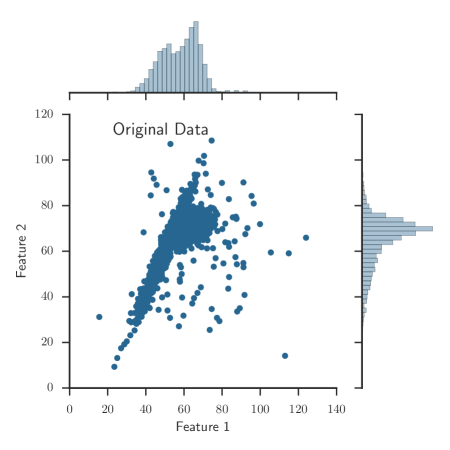
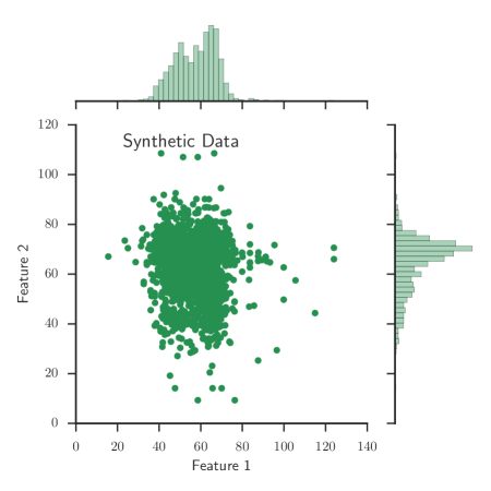
Since the objects in our sample are not labeled and there is no external information input to the algorithm from the user, we perform unsupervised learning with RF, as described in Shi & Horvath (2006) though with some key modifications. We construct a synthetic data matrix with the same dimensions as our sample data (2 355 926 X 15 700): each feature (column) in the synthetic data is built by sampling from the marginal distribution of the same feature in the original data. The process of creating the synthetic data is illustrated in figure 2 in a simplified example, where each object has only two features, distributed as seen in the left panel. The synthetic data is shown in the right panel, where one can see that the marginal distributions of the original and synthetic data match, while the covariance between the features remains only in the original data.

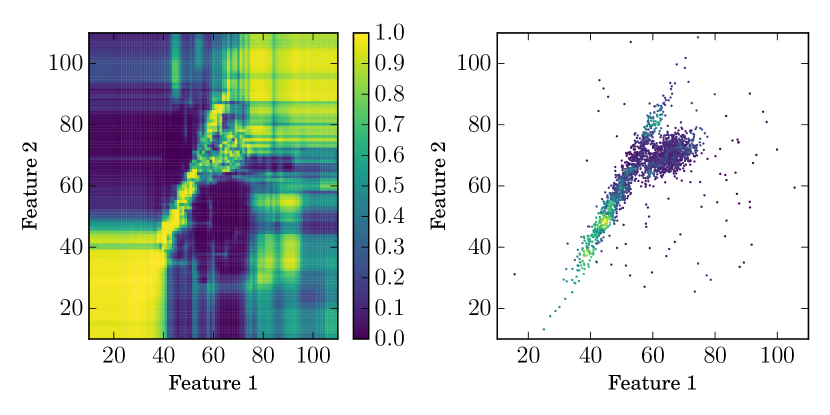
Once we have the synthetic data, we can translate the problem to the language of supervised learning – we label the original data as real and the synthetic data as synthetic. The total labeled data which consists of both the real and synthetic samples is the input to the traditional RF classification algorithm. We note that there is no need to divide the sample into training, validation, and test sets as typically done when performing supervised learning, since we do not use the trained forest as a predictor for new, unlabelled, measurements. We train the forest to distinguish between real and synthetic, and since the difference between the classes is the lack of covariance in the synthetic data, the forest identifies features which show strong covariance and rates them higher in its features importance scheme. In this framework, spectral lines will show as correlations on short scales, between nearby wavelengths, while continuum slopes manifest themselves as more subtle correlations (typically) between distant wavelength ranges. Noise is largely uncorrelated, except perhaps for the influence of the point-spread-function that introduces short-range correlations in spectra. We apply the RF training to the illustration data from figure 2 and show in the left panel of figure 3 the probability of an object to be classified as real by the trained RF. One can see that although the real and synthetic data occupy the same region in parameter space, the RF learns the region of the real objects well.

Figure 4: Histogram of the weirdness score for every object in our sample. One can see that the distribution is smooth and decreases as one approaches large values. We study in this paper the 400 objects that lie to the right of the dashed blue line.

Figure 5: Histogram of the signal to noise ratio (SNR) of the galaxies in our sample. We define the SNR as the median SNR per pixel, as given by the SDSS pipeline. One can see that apart from a prominent peak in the distribution at SNR$\sim$2.5, the number of galaxies decreases smoothly for increasing SNR.

Having the trained forest, we take only the real objects and propagate them through the decision trees in the forest. Every object, in every tree, ends up in a terminal node (leaf) with a predicted class, either real or synthetic. In order to define a measure of similarity between objects, we count how often every pair of objects were classified as real in the same leaf of a given tree. This number, $\mathrm{N_{leaf}}$, can range from 0 to the number of trees in our forest. $\mathrm{N_{leaf}}$ is a measure of the similarity between these two objects since objects that have a similar path inside the decision tree have similar features, and as a consequence are represented by the same model. We normalise $\mathrm{N_{leaf}}$ by dividing it by the number of trees in the forest which classify both objects as real, $\mathrm{N_{trees}}$, giving us a similarity measure for every pair of objects. We define the distance between objects $i$ and $j$ as: $D_{ij}=1-\mathrm{N_{leaf}/N_{trees}}$. $D_{ij}$ can range from 0 (objects that ended up in the same leaf in all the trees), which is the distance of an object to itself, to 1 for objects that never ended up in the same leaf.

We note that the standard way to measure distances between objects with RF is counting the number of tress in which the objects ended up in the same leaf, regardless of the leafs prediction (e.g., Shi & Horvath 2006), in this case $\mathrm{N_{trees}}$ is constant and equals to the number of trees in the forest. However, we find that the quality of the outliers improves when taking into account only leaves that predict both of the objects to be real. This may be due to the fact that a model (the path in a decision tree) that describes a synthetic object does not describe well a real object and vice versa. The galaxies in our sample are classified as synthetic by a decision tree with a probability of up to 25%. This probability depends on the SNR of the galaxies, such that the probability to be classified as synthetic increases with decreasing SNR. We note however that each decision tree has access to a limited number of features and therefore a galaxy with high SNR can be classified as synthetic in some subset of the trees, thus adding noise to the distance measure. We further refer the reader to the work by Shi & Horvath (2006), where they discuss different methods of synthetic data construction, distance assignment, and discuss the difference and similarity to the Euclidean distance.

Using this distance measure, we can cluster the objects but our purpose is to find outliers. The distance between all the pairs of objects is a matrix with dimensions 2 355 926 X 2 355 926, more than 20TB in double precision. Since we are interested in outlying objects, which have a large distance from most of the other objects in the dataset, it is enough to average the distances of a given object to all the others, resulting in a 2 355 926-sized vector that represents the ‘weirdness’ score of each object. This vector is of a reasonable size and we can sort it and extract the objects with the highest weirdness score from the entire population – the outliers. The sorted vector of averaged distances essentially orders the galaxies from the most mundane, with a weirdness score of 0, to the most unusual, with a score of 1. Therefore, the threshold for the outlying objects is user-defined. We also note that due to the randomness of the RF in its feature and object selection, the decision trees vary from one run to the next, and the weirdness score that we obtain is not unique. However, we find that when using a sufficient number of decision trees (see details in section 3.1) an object with a high weirdness score in one run will have a high weirdness score in different runs as well.

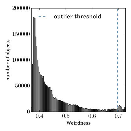
We measure the weirdness score for the illustration data shown in figure 2 and show it in the right panel of figure 3, where dark blue represents objects with high weirdness score and yellow represents objects with a low weirdness score. One can see that objects that are located in the tail of the distribution and noisy points tend to have higher weirdness scores. We show in figure 4 a histogram of the weirdness score for all the galaxies in our sample. One can see that the distribution is smooth and decreases monotonically with the weirdness score. The presence of peaks in the histogram would have implied the existence of clusters of objects, composed of galaxies which have a short distance to the cluster members, but a long distance to galaxies in different clusters. The smoothness of the distribution that we measure may imply that the classifier is sensitive even to small differences between seemingly similar galaxies. This is essentially over-fitting, which is typically bad for supervised algorithms that are expected to generalise well to new measurements, but serves our purpose to find outliers. Alternatively, a smooth distribution in the averaged distance can happen if the galaxy spectra form a continuous sequence in spectral shape (e.g., Ascasibar & Sánchez Almeida 2011). In Section 4 we analyse the 400 weirdest objects, which lie to the right of the dashed blue line.

Figure 6: Distributions of the classes of outlying objects we find. Clearly, we find a wide variety of phenomena. It is interesting that only a small fraction (2.5%) are due to instrumental problems.

Figure 7: SDSS J135338.10+313325.1 (2117-54115-230) has a number of velocity components in its Balmer and forbidden lines. There are two $\mathrm{[OIII]}$ emission peaks and another blue-shifted component, probably due to an outflow (left panel). In the Balmer emission lines one can see a broad component that is redshifted (see right panel). The vertical dashed lines mark the rest-frame central wavelength of emission lines, based on the redshift estimation of the SDSS pipeline.

3.1 Implementation

As noted above, RF is a naturally parallelisable algorithm due to the randomness of its object and feature selection. The size (2 $\times$ 2 355 926 objects) and complexity (15 700 features) of our data prevent us from applying this algorithm with the entire data loaded to memory and the analysis to be done with a single process. Instead, we break the data into 8 bins of signal to noise ratio (SNR) of equal size, each bin contains roughly 300 000 galaxy spectra. We define the SNR of a spectrum as the median SNR per pixel, as given by the SDSS pipeline.

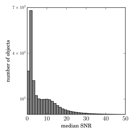
In addition to shorter running time, we find that dividing the spectra into SNR bins improves the quality of the outliers we find. We show the distribution of galaxy SNR in the SDSS in figure 5, where one can see a smoothly declining distribution, except for a prominent peak at SNR$\sim$2.5 (with roughly 700 000 galaxies). Like other machine-learning classifiers, RF builds a model that is mostly sensitive to the common object in the sample while objects that are rare are not well described. Therefore, when training without SNR bins, the decision trees are optimised to distinguish between real and synthetic data for a galaxy with SNR$\sim$2.5, but not for galaxies with higher SNR. In practice, the decision trees rank wavelengths with prominent emission lines such as $\mathrm{H\alpha}$ and $\mathrm{[OIII]}$ high in the feature importance ranking, while ignoring the weaker emission lines such as $\mathrm{H\beta}$, $\mathrm{[SII]}$, and $\mathrm{[OI]}$, and ignoring absorption lines, since the information of a galaxy with SNR$\sim$2.5 is mostly contained in these strong emission lines. We therefore divide the sample into SNR bins and indeed find that the feature importance of weak emission lines and absorption lines increases for bins of higher SNR, while prominent emission lines are ranked high in all of the bins.

Within a given SNR bin, we build 50 redundant chunks which contain 10 000 objects, and while the galaxy spectra within a given chunk are unique, a specific galaxy spectrum can be included in several different chunks. We construct 200 decision trees for each of these chunks, while using only a subset of the features in the construction of a single tree (a square root of the number of features is used for a given decision tree, which is a typical choice). Therefore, for a given SNR bin we build 10 000 decision trees while using 125 features for each tree. We test different numbers of objects per chunk and find that for 5 000 – 20 000 galaxies in a chunk the weirdness score distribution is the same, resulting in the same quality of outliers. However, when using 1 000 – 3 000 galaxies per chunk the result is degraded (e.g., supernovae and stars do not always have a high weirdness score, and standard galaxies sometimes have a high weirdness score), and the distribution in weirdness score appears flatter. We also note that increasing the number of decision trees for a fixed number of observations generally results in a better and more general classifier but increases the training time substantially. For our dataset, we find that the distribution in weirdness score stabilises and barely changes once we reach 200 trees per 10 000 objects. This process is identical to the RF training procedure we presented in section 3 and the construction of decision trees per chunk is executed in parallel on multiple computer nodes. We use the decision tree classifier and RF classifier implementation in scikit-learn (Pedregosa et al. 2011).

Once we have the decision trees from the parallel processes, we merge them into a forest. The phase of propagating an object through the trees and comparing its leafs to that of the other objects is done in parallel as well. The parallelisation in this case is object based – we pair the reference object with all the other objects and compute the distance between the reference object to the entire sample and then we average it. These details were tailored to the data at hand, and to our available computational resources. We stress that they affect execution time but not our scientific results. In total the process takes 12 hours on 128 CPUs to obtain the weirdness score. The bulk of our computations was performed on the resources of the National Energy Research Scientific Computing Center.

3.2 Dimensionality reduction

Dimensionality reduction and feature selection methods are often proposed when dealing with large-size and complex data. The goal of dimensionality reduction techniques is to extract the strongest, most prominent features in the data and use them for classification or regression problems. These methods assume that the data can be well represented in a lower dimensional space, thus allowing for faster and (sometimes) better statistical inference. A common method is Principal Component Analysis (PCA) which performs a linear decomposition of the data and provides eigenvectors and their strength coefficients for every object in the dataset (e.g. Zhang et al. 2006; Vanden Berk et al. 2006; Rogers et al. 2007; Re Fiorentin et al. 2007; Bailey 2012). When modelling a spectrum, the linearity of PCA may be a disadvantage due to the nonlinearity of spectral lines. Thus, it is not clear that applying PCA prior to the forest construction is beneficial for our algorithm.

Nevertheless, we apply PCA decomposition on the 10 000-sized chunks and use the coefficients provided by the decomposition as the features for the forest construction and outlier detection. We test different number of input coefficients: using 10 000, 5 000, 2 000, 1 000, 500, and 100. In all the cases the result suffers. Outlying objects tend to have a few coefficients with large (positive and negative) values, compared to the values for the same coefficients of standard objects. These large coefficients are not modelled well by the forest and tend to fall in the same leaf of a given decision tree, thus appearing similar to each other. Standard spectra which are intrinsically alike also tend to fall in the same leaf and appear similar. These two groups (intrinsically similar objects and outlying objects) show the same summed distances and therefore cannot be separated with a distance criterion. So while PCA might be advantageous for a classification problem with RF, by mitigating over-fitting, it impairs our weirdness measure.

There are dimensionality reduction algorithms which are not linear. Richards et al. (2009) apply diffusion maps to galaxy spectra for data parametrisation and dimensionality reduction prior to using the spectra in a regression problem. Vanderplas & Connolly (2009) and Daniel et al. (2011) use Locally Linear Embedding (LLE) as a nonlinear dimensionality reduction technique for classification of SDSS spectra. Although these methods show great promise in the dimensionality reduction field, we chose not to use them since RF, contrary to many ML algorithms, deals with large number of features well, and applying these methods is expensive both in terms of running time and available memory. Furthermore, it is not trivial to apply these methods on millions of objects in the DFS framework and on data streams. More importantly, as noted above, the better they work, the more they are likely to harm our algorithm for outlier detection.

3.3 Comparison with other outlier detection algorithms

There are several outlier detection algorithms that are based on unsupervised learning which are widely used in various fields. These algorithms can be divided into two types. The first type is distance-based anomaly detection, in which a distance is computed between every pair of objects in the sample and outliers are defined as objects that are distant from most of the objects in the sample. This includes Euclidian-based distance assignment, PCA-decomposition-based distance assignment, and unsupervised RF distance assignment. The running time of these algorithms scales as $\mathrm{O(N^{2})}$, where $\mathrm{N}$ is the number of objects in the sample, since a pairwise distance must be computed. The second type of algorithms focus on isolating outliers rather than modelling the entire data and defining outliers as objects that deviate from this model. The most popular such algorithm is Isolation Forest (iForest; Liu, Ting & Zhou 2008). Such algorithms are typically linear in time. We refer the reader to Liu, Ting & Zhou (2008) and Goix (2016) for comparison between different algorithms for different data-sets.

We compare the quality of the outliers we find with the following algorithms: One-Class SVM (Schölkopf et al. 1999), iForest (Liu, Ting & Zhou 2008), standard unsupervised RF (Shi & Horvath 2006), and our method introduced here. While our method is distance based, it is not as fast as iForest for example, but it is naturally parallelisable, reducing wall-time. We gauge the quality of the outliers we find with the various methods qualitatively, using domain knowledge. For example, we expect supernovae and stars to have high weirdness scores, and galaxies that are only brighter but otherwise normal to have low scores. We also compare the number of false-positives found by these algorithms, that is the number of standard-looking objects that are marked as outliers by the algorithms.

Visually inspecting the 400 weirdest galaxies found by each of these algorithms, we find that our method significantly outperforms the others, finding essentially only interesting galaxies, as thoroughly discussed below. The standard unsupervised RF algorithm tends to pick a larger number of false-positives. For One-Class SVM and iForest the galaxies that are found as outliers include mostly galaxies with residual cosmic rays, galaxies with extremely strong emission lines, stars, and a few false positives. Generally, we find that these algorithms detect objects that show outlying properties in specific features (i.e., wavelengths) but are not sensitive to outlying relation between features such as extremely reddened galaxies, outlying line ratios, and unusual emission lines. Although the former are indeed outliers in a statistical sense, the covariance-based outliers are more interesting and offer the opportunity to discover subtle changes that represent an outlying physical behaviour.

Figure 8: Two examples of galaxies with an additional structure near the H↵-[NII] complex. SDSS J013402.54-094627.0 (663-52145-306; top panels) has an unusual asymmetric emission near $\mathrm{H\alpha}$ and no emission near $\mathrm{H\beta}$. SDSS J124144.54+350345.9 (2022-53827-286; bottom panels) has a more symmetric structure, with a centroid that is slightly shifted from the $\mathrm{H\alpha}$ wavelength. In both of the cases we find similar structure in $\mathrm{H\beta}$ after we subtract the best stellar population synthesis model, though we do not detect continuum emission from an accretion disk.

4 Outlying Galaxies

We systematically inspect the 400 weirdest galaxies that we find. We caution the reader that their relative numbers are not very meaningful, since our choice to study 400 is arbitrary, and limited by the time necessary to inspect all the aspects of each galaxy, as we do below. This includes visual inspection of the SDSS spectrum and imaging, line measurements where applicable, a literature search (since this sample was so extensively studied), and other more specific measurements for specific cases. There are undoubtedly many more interesting sources with a marginally lower weirdness score. We encourage our readers to explore further. A table with a weirdness score for all the 2M galaxies is available at http://www.wise-obs.tau.ac.il/$\sim$dovip/weird-galaxies/, and an IPython notebook with the algorithm is available at https://github.com/dalya/WeirdestGalaxies.

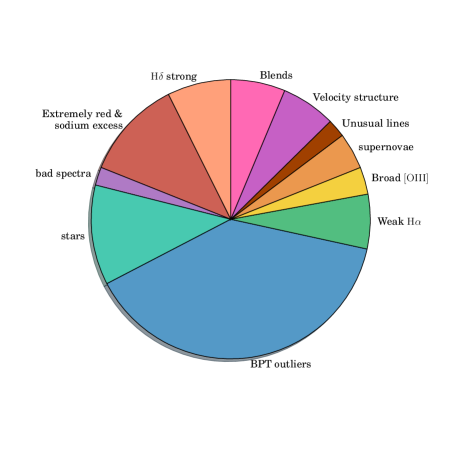
Out of 400, we call 10 objects ‘bad spectra’ and they consist of objects with calibration problems and sky contamination, we find 47 stars classified as galaxies by the SDSS pipeline. 27 objects we call ‘blends’, which includes galaxy-galaxy lenses, chance alignment of two objects, and multiple emission line systems. We find 186 galaxies with unusual emission-line ratios. 13 galaxies sport an unusually broad [OIII] emission, in fact, it is so broad in some cases that the SDSS pipeline mistakes it for a broad $\mathrm{H\alpha}$ emission line at a wrong redshift. We also find 33 galaxies with extreme Balmer absorption up to $\mathrm{H\delta}$ and beyond, and 38 objects with an excess of NaID absorption. 18 outliers are galaxies that host supernovae, 9 show unusual emission lines (e.g., coronal lines, $\mathrm{[NI]}$). We find 41 galaxies with unusual velocity structures – 11 of them show an additional structure around the $\mathrm{H\alpha}$-$\mathrm{[NII]}$ complex, and 13 show double-peaked emission lines. We show in figure 6 a pie chart that summarises all the outlying objects and their classification. Out of the 400 outliers, only 74 outliers were previously reported by other studies – in all of these cases the authors have constructed a specific algorithm that is tailored exactly to find the kind of objects they are looking for. We list all the outlying galaxies in appendix A with classification and references to previous studies when relevant. Throughout this section, we note specific galaxies with their SDSS name (e.g., SDSS J131027.46+182617.4) and their SDSS PLATE-MJD-FIBER.

4.1 Unusual velocity structure

We find 42 galaxies with an unusual velocity structure in their emission lines. Out of these, 11 galaxies show an additional structure around the $\mathrm{H\alpha}$-$\mathrm{[NII]}$ complex, 13 galaxies have double-peaked emission lines, three show two broad components in the $\mathrm{H\alpha}$ and $\mathrm{H\beta}$. We also find 13 galaxies with unusually broad $\mathrm{[OIII]}$ emission, and the remaining five galaxies show a number of interesting velocity components in their emission lines. We list these five objects in table 1.

We present in figure 7 one of the four galaxies that shows the most complex velocity structure as an example. SDSS J135338.10+313325.1 (2117-54115-230) has a number of velocity components in its Balmer and forbidden lines. We mark the rest-frame wavelengths of the emission lines based on the redshift estimation of the SDSS. One can see that this galaxy has two $\mathrm{[OIII]}$ emission peaks and another blue-shifted component, probably due to an outflow. In the Balmer emission lines one can see a broad component that is redshifted compared to the central rest-frame wavelength (more prominent in the $\mathrm{H\alpha}$ emission). The galaxy seems disturbed in the SDSS imaging, and this velocity structure could arise from asymmetries near the centre of the galaxy which is picked up by the spectroscopic fibre. We also note SDSS J113818.38+060620.1 (4767-55946-889), which has an ultra-luminous, galaxy-wide narrow line region and is studied by Schirmer et al. (2013) as it is a ”green bean”. Schirmer et al. (2013) construct a sample of 29 such galaxies from SDSS DR8, and claim them to be among the rarest objects in the universe.

4.1.1 Additional structure near $\mathrm{H\alpha}$

We find 11 objects with an additional structure near the $\mathrm{H\alpha}$-$\mathrm{[NII]}$ complex. The stellar continuum contribution in these galaxies is stronger than nebular emission, mostly near $\mathrm{H\beta}$, thus similar features are not easily detected in $\mathrm{H\beta}$ emission. In order to isolate the emission of the gas from the stellar component, we subtract the best fitting population synthesis model for each of the galaxies. We use pPXF (Cappellari 2012), which is a public code that extracts the stellar kinematics and stellar population from absorption-line spectra of galaxies (Cappellari & Emsellem 2004). The code uses the MILES library, which contains single stellar population synthesis models from Vazdekis et al. (2010). In several galaxies, we obtain unrealistic stellar population fits due to the broad $\mathrm{H\alpha}$ emission. We therefore ignore pixels that are dominated by the broad emission features prior to the fitting, and obtain good fits.

Figure 9: Example of an object with double-peaked emission lines in the observer frame (SDSS J163228.43+541449.2; 6788-56428-257). The object shows two strong sets of emission lines which are separated by 700 $\mathrm{km\,s^{-1}}$ (black line). The SDSS pipeline estimate the redshift of the object to be $z=0.214$, fitting a model where a broad $\mathrm{H\alpha}$ component accounts for the wide and double $\mathrm{[OIII]}$ line (SDSS model in pink). We estimate the redshift of the emission line components to be $z=0.590$ and $z=0.594$, and mark the $\mathrm{[OIII]}$ and $\mathrm{H\beta}$ emission line wavelengths in the observers frame according to our redshift estimation. The galaxy shows extremely symmetric components, compared to other double-peaked emission line galaxies, which may indicate that we are seeing a disk-like structure.

The emission spectra of these galaxies show a wide range of properties. For some of the galaxies, we detect a similar emission structure around $\mathrm{H\beta}$, suggesting that the broad features are due to Balmer emission, and in some of these the broad emission is not centred around the central wavelength of the narrow emission, suggesting an outflow or a complex geometry (e.g., SDSS J154327.02+075442.1, 1724-53859-116, which shows an outflow in the Balmer emission lines). We find that several galaxies show diagonally-shaped continua (see section 4.5.2), which suggests that the broad $\mathrm{H\beta}$ emission is absorbed by dust reddening and is not detected due to our limited SNR. Furthermore, we find that while for five of the galaxies the additional structure can be attributed to a broad $\mathrm{H\alpha}$ emission, or to two $\mathrm{H\alpha}$ velocity components which are blended, the remaining six show asymmetric structures which cannot be described by a broad Gaussian. We list these objects in table 2.

Figure 10: Histogram of the FWHM of the forbidden emission lines of galaxies from the MPA-JHU catalogue (left panel), compared to the FWHM of the $\mathrm{[OIII]}$5007Å  emission line we measure for our objects. One can see that our objects reside in the tail of the width distribution. As an example, we show SDSS J165205.39+430902.3 (6031-56091-0007; right panel; black), $z=0.634$, where $\mathrm{H\beta}$, $\mathrm{[OIII]}$4959Å, and $\mathrm{[OIII]}$5007Åare marked with blue dashed lines. The FWHM of $\mathrm{[OIII]}$5007Å  is $930\,\mathrm{km\,s^{-1}}$ (pink).

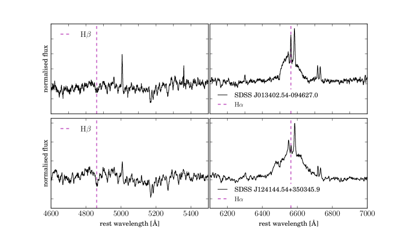
We present two examples of such objects in figure 8. SDSS J013402.54-094627.0 (0663-52145-0306; top panels) shows an asymmetric profile, which cannot be well represented by a single or double Gaussian and is not centred around the $\mathrm{H\alpha}$ emission line. After subtracting the best stellar population synthesis model from the spectrum, we detect two broad emission components around $\mathrm{H\beta}$, which suggests that the broad feature around $\mathrm{H\alpha}$ is due to Balmer emission (rather than $\mathrm{[NII]}$ emission or a mix of the two). However, using two broad emission components for $\mathrm{H\alpha}$ (and all the narrow emission lines) we are not able to reproduce the shape of the emission we observe. We find that adding an additional broad component in absorption can reproduce the profile we observe. Broad Balmer absorption is typically seen in Type II supernovae ejecta (see for example Faran et al. 2014) or extremely dense outflows in high redshift quasars (see Williams et al. 2016 and references therein). An alternative interpretation for this profile is a circular, relativistic, Keplerian disk which is observed in a small fraction of AGN (Eracleous & Halpern 2003). SDSS J124144.54+350345.9 (2022-53827-0286; bottom panels of figure 8) has a more symmetric structure, only slightly shifted from the $\mathrm{H\alpha}$ wavelength. We detect the same structure in $\mathrm{H\beta}$ after subtracting the stellar population contribution. In both of these cases, we do not detect continuum emission from an accretion disk.

4.1.2 Double-peaked emission line galaxies

Another subset of objects consists of galaxies with double peaked emission lines, of which we find 13, 10 of which show narrow and 3 show broad double-peaked emission lines. Previous studies conducted searches in the SDSS spectroscopic data with the purpose of finding double peaked emission lines in galaxies and AGN up to the seventh data release (DR7; Wang et al. 2009; Liu et al. 2010; Smith et al. 2010; Ge et al. 2012; Pilyugin et al. 2012 and references therein). Smith et al. (2010) searched for binary AGN and by visual inspection of SDSS AGN spectra found 148 spectra with a double peaked $\mathrm{[OIII]}$ profile. Pilyugin et al. (2012) looked for galaxies with two simultaneous starbursts and by visual inspection of the SDSS spectra found a few hundreds of galaxies with double peaked emission lines, and studied 55 of them, which had a reliable two component decomposition. Ge et al. (2012) compiled the first systematic sample of 3030 double peaked emission lines objects.

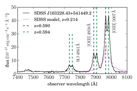
Out of the 10 galaxies with double-peaked narrow emission lines, two were reported by previous studies. SDSS J103007.07+412353.5 (1360-53033-0186) is part of the sample presented by Pilyugin et al. (2012) and Ge et al. (2012). SDSS J131642.90+175332.6 (5867-56034-0304) is discussed specifically by Xu & Komossa (2009), where the authors suggested and discussed a few scenarios which can potentially account for the double peaked profiles of all of the lines, such as a binary AGN, galaxy merger, and jet-cloud interaction. This object is of a particular interest since it shows double emission profiles in all its nebular lines and an additional broad component (FWHM of $1400\,\mathrm{km\,s^{-1}}$) in most of its forbidden lines. Two additional objects (out of the 10) are worth noting since the SDSS pipeline failed to estimate their redshift correctly: SDSS J223623.78+112824.0 (5049-56103-0273) and J163228.43+541449.2 (6788-56428-0257). The velocity separation between the two peaks is $550\,\mathrm{km\,s^{-1}}$ and $710\,\mathrm{km\,s^{-1}}$, higher compared to the velocity separation of double-peaked galaxies (see velocity separation distribution in Pilyugin et al. 2012). We present, as an example, the object SDSS J163228.43+541449.2 in figure 9 (black) compared to the best fitting model of the SDSS pipeline (pink) which mistakes the redshift to be $z=0.214$, identifying the broad $\mathrm{[OIII]}$ line as $\mathrm{H\alpha}$. We estimate the redshift of the two emission line components to be $z=0.590$ and $z=0.594$ with a velocity separation of $710\,\mathrm{km\,s^{-1}}$. These galaxies were not reported in previous studies.

We find 3 galaxies which show double-peaked broad emission lines, all of them are reported by previous studies as well. Due to this structure, the SDSS pipeline fails to fit a correct redshift to two of them, fitting the broad double-peaked $\mathrm{H\alpha}$ emission as $\mathrm{Ly\alpha}$ emission. For SDSS J013253.31-095239.3 (662-52147-180), the SDSS estimate the redshift to be 5.73, while we measure it to be 0.259. The broad emission components belong probably to $\mathrm{H\alpha}$ emission (and not the $\mathrm{[NII]}$) since we observe the same structure in $\mathrm{H\beta}$. These components are located at a velocity of 2880 $\mathrm{km\,s^{-1}}$ (blue-shifted) and -4890 $\mathrm{km\,s^{-1}}$ (redshifted). SDSS J114051.58+054631.1 (838-52378-460) also show two broad emission lines, offset by 4600 $\mathrm{km\,s^{-1}}$ and -5800 $\mathrm{km\,s^{-1}}$, and we estimate its redshift to be 0.131. For additional information, we refer the reader to the studies that discovered and studied these objects: Strateva et al. (2003), Wu & Liu (2004), Bian et al. (2007), and Strateva et al. (2008). We list all the double-peaked galaxies in table 3.

4.1.3 Broad $\mathrm{[OIII]}$ emission line

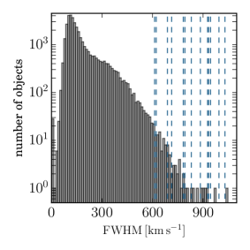
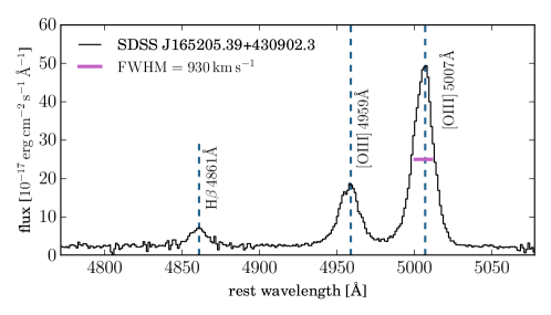
We find 13 galaxies with relatively broad $\mathrm{[OIII]}$ emission lines. For 4 of these objects the SDSS pipeline fails to fit a model with a correct redshift, identifying the unusual $\mathrm{[OIII]}$ as $\mathrm{H\alpha}$. We derive the redshift of the objects by fitting the $\mathrm{H\beta}$, $\mathrm{[OIII]}$4959Å, $\mathrm{[OIII]}$5007Å  complex, with just three Gaussians, and extract the FWHM of the $\mathrm{[OIII]}$ 5007Å  line. The values we derive range from $600\,\mathrm{km\,s^{-1}}$ to $1000\,\mathrm{km\,s^{-1}}$.

In order to compare the FWHM of our $\mathrm{[OIII]}$5007Å  emission line to that of the general population, we use the MPA-JHU catalogue, which contains emission line measurements of 927 552 galaxies from SDSS DR7 (Kauffmann et al. 2003b; Brinchmann et al. 2004; Tremonti et al. 2004). They also derived the velocity of all the forbidden lines (they constrained the velocity to be the same in all the forbidden lines in their fitting process) and converted it to FWHM value, assuming a Gaussian profile. We use galaxies for which the velocity measurement is at least three times higher than its uncertainty, thus rejecting low SNR objects. We show in the left panel of figure 10 the histogram of the FWHM of the entire galaxy population compared to the FWHM of our objects. One can see that these objects are located on the tail of the distribution of the entire population. As an example, we present SDSS J165205.39+430902.3 (6031-56091-0007) in the right panel (black). The redshift derived by the SDSS is $z=0.244$ while the redshift we derive is $z=0.634$, and we measure a FWHM of $930\,\mathrm{km\,s^{-1}}$ for the $\mathrm{[OIII]}$ emission line. We note that in the case of broad $\mathrm{[OIII]}$ emission, samples constructed from the SDSS can be incomplete and biased due to incorrect redshift estimation. At a redshift of $z\sim 0.5$, where $\mathrm{H\alpha}$ is outside the SDSS wavelength range, broad $\mathrm{[OIII]}$ emission can be confused with broad $\mathrm{H\alpha}$ and $\mathrm{Ly\alpha}$ emission, and indeed there are hundreds of quasars with incorrect redshift estimation in the SDSS database (see Reyes et al. 2008 and Yuan, Strauss & Zakamska 2016). We list the broad $\mathrm{[OIII]}$ emission line galaxies in table 4.

Figure 11: SDSS J132401.63+454620.6 (1463-53063-262) – $\mathrm{H\delta}$ strong galaxy which also has a broad $\mathrm{H\alpha}$ emission line (left panel). This object is peculiar since the strength of the $\mathrm{H\delta}$ indicates a recent change in its star formation activity, however an AGN is still detectable through broad $\mathrm{H\alpha}$ emission. We fit the lines (right panel), find that the FWHM of the broad $\mathrm{H\alpha}$ component is $2150\,\mathrm{km\,s^{-1}}$, and that the line ratio $\mathrm{log\,[NII]/H\alpha}=0.28$ is consistent with gas that is exposed to hard X-ray radiation.

In many galaxies, the $\mathrm{[OIII]}$ emission lines show an additional blue-shifted component, which is usually interpreted as being due to outflows. Forbidden lines are used to study the kinematics of galaxies, since in most of the cases they have narrow resolved profiles (unlike the $\mathrm{H\alpha}$ and $\mathrm{H\beta}$ for example). As a consequence, different velocity components can be separated and studied. However, broad $\mathrm{[OIII]}$ lines that can be well described by a single Gaussian are rare (e.g., Alexander et al. 2010; Greene et al. 2011; Harrison et al. 2014; Carniani et al. 2015; Zakamska et al. 2016).

4.2 E+A galaxies

E+A galaxies (also known as k+a galaxies, ‘post-starburst’, and $\mathrm{H\delta}$-strong galaxies) are galaxies with strong Balmer $\mathrm{H\delta}$ absorption in their spectra, with values typically larger than 4–5Å. The emission in these galaxies is dominated by A-stars, with lifetimes of around one Gigayear. Therefore, stars were formed recently, O-stars and B-stars have all evolved past the main-sequence, but A-stars have not yet. Consequently, E+A galaxies must have undergone a recent (and quite abrupt) change in their star formation. These galaxies comprise 3% of the general galaxy population (Goto et al. 2003) and in many of them it appears that a significant fraction of the galaxy stellar mass was created in the starburst (20-–60%). A special sub-class of these are galaxies that do not show $\mathrm{H\alpha}$ and $\mathrm{[OII]}$ emission lines, indicating that these galaxies are not currently star forming, but have undergone a recent starburst. These galaxies are observed during a short-lived phase in their evolution, and are fewer than 1% of the galaxy population (Goto et al. 2003; Goto 2004; Balogh et al. 2005; Goto 2007; Melnick & De Propris 2013; Alatalo et al. 2016).

Out of 400 outlying galaxies, we identify strong $\mathrm{H\delta}$ absorption in 33, 28 of which were discussed in previous studies of such galaxies (see references above). We look for $\mathrm{H\alpha}$ and $\mathrm{[OII]}$ emission in our objects and find that only 7 out of 33 show emission lines that indicate ongoing star formation, while 26 do not. We list the $\mathrm{H\delta}$ strong galaxies we find in table 5.

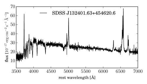
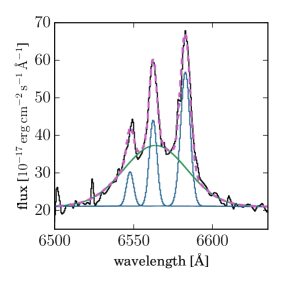
We note specifically SDSS J132401.63+454620.6 (1463-53063-262), which shows strong $\mathrm{H\delta}$ absorption and a broad emission components near the $\mathrm{H\alpha}$ emission line. We show the object in the left panel of figure 11. We start by fitting a stellar population synthesis model to account for the stellar continuum, like in Section 4.1.1. We find a good fit with a population of stars of age 0.05–0.1 Gigayear, as expected for E+A galaxies. We then subtract the stellar contribution in order to study the properties of the emitting gas.

We start by fitting a single component to the narrow $\mathrm{H\alpha}$ emission and two additional narrow components to the $\mathrm{[NII]}$ emission and find that these cannot account for the entire emission. We therefore fit an additional, broad, component that is centred around the $\mathrm{H\alpha}$ central wavelength. The best fitting profile is presented in the right panel of figure 11. The FWHM we obtain for the broad $\mathrm{H\alpha}$ is $2150\,\mathrm{km\,s^{-1}}$. We also measure the line ratio $\mathrm{log\,[NII]/H\alpha}$ for the narrow components and find it to be 0.28, consistent with gas that is exposed to hard X-ray radiation. We note however that the forbidden lines $\mathrm{[SII]}$, $\mathrm{[OI]}$, and $\mathrm{[OIII]}$ show weak broad features that are marginally detected, thus it is possible that the broad emission around $\mathrm{H\alpha}$ is composed of both $\mathrm{H\alpha}$ and $\mathrm{[NII]}$ contributions.

It is clear that this object is of special interest. The stellar composition of the galaxy suggests that star formation has started simultaneously in the entire galaxy (due to the narrow age distribution that we find) and that the galaxy has undergone a recent shut-down of its star formation (i.e., no O-stars and B-stars). On the other hand, we measure broad emission components that may suggest either AGN heating or shocked gas due to recent merger or nuclear outflows. In terms of the cosmic cycle (e.g., Hopkins et al. 2006), this galaxy may represent a very short-lived phase in general galaxy evolution, where the star formation had already terminated due to AGN feedback though enough gas is still left to fuel the accretion disk (see for example Springel, Di Matteo & Hernquist 2005 and Netzer 2009). Studying this galaxy and similar ones may allow one to study the feedback mechanisms that terminate star formation, which we do in Baron et. al. (in prep).

Figure 12: Galaxy with detected high ionisation emission lines. SDSS J120041.39+314746.2 (6473-56363-672) is a galaxy at redshift $z=0.116$ for which we detect the coronal lines: [FeX] 6376Å, [FeVII] 6088Å, [FeVII] 5722Å, [FeXIV] 5304Å, and [FeVII] 3759Å. This galaxy is not reported by Wang et al. (2012) since it is classified as AGN from its line diagnostics.

Figure 13: An example of a galaxy with unusually strong $\mathrm{[NI]}$ emission. SDSS J102339.63+041110.6 (575-52319-200) is a galaxy at redshift $z=0.290$ and it is a member of a galaxy cluster, and it is detected in radio emission. We measure the ratio $\mathrm{[NI]/H\beta}=0.33$ in the spectrum, while in planetary nebulae the $\mathrm{[NI]}$ emission is 10–100 times weaker than $\mathrm{H\beta}$.

4.3 Unusual emission lines

We find 3 galaxies that show coronal lines in their spectra, and 10 galaxies with strong $\mathrm{[NI]}$ 5200Å  emission. We list these galaxies in table 6.

4.3.1 Coronal line emitters

High-ionisation, or coronal lines arise in gas that is exposed to soft X-ray radiation. Several studies have suggested a connection between extreme coronal line emitters (ECLEs) and tidal disruption events (TDE), in which a star is tidally disrupted as it enters the tidal radius of a massive black hole (Komossa et al. 2008; Wang et al. 2011, 2012). Wang et al. (2012) were the first to conduct a systematic search for TDEs in the SDSS spectroscopic data by looking for ECLEs. They detected ECLEs by either looking for extreme coronal lines (at least one line is at least 20% as strong as the $\mathrm{[OIII]}$ line) or coronal lines from a galaxy that is classified as an HII region on the BPT diagram. The authors found 7 objects in total that satisfy the criteria, one of them is found as an outlier by our algorithm (SDSS J093801.63+135317.0; 2580-54092-0470). It is worth noting that out of the 7 objects in their sample, only 4 objects are classified as galaxies by the SDSS pipeline (rather than QSO) and enter our sample.

Figure 14: BPT diagrams based on the $\mathrm{[NII]/H\alpha}$ and $\mathrm{[OIII]/H\beta}$ emission line ratios (left panel) and $\mathrm{[SII]/H\alpha}$ and $\mathrm{[OIII]/H\beta}$ ratios (right panel). The grey background represents the density of SDSS galaxies (927 552 galaxies from DR7), on a logarithmic colour scale. Outlying galaxies are marked with green circles. Outlier galaxies which are classified as HII regions in one diagnostic and as AGN in another are each plotted with the same marker and colour in both panels. The classification limits are taken from the extreme starburst limit by Kewley et al. (2001) (Ke01; blue line) and composite galaxies by Kauffmann et al. (2003b) (Ka03; black line).

We find two additional galaxies with coronal lines ([FeX] 6376Å, [FeVII] 6088Å, [FeVII] 5722Å, [FeXIV] 5304Å, [FeVII] 3759Å), these galaxies do not meet the criteria of Wang et al. (2012), since they are classified as AGN in the BPT diagnostic diagram. We show an example of such galaxy, SDSS J120041.39+314746.2 (6473-56363-672), in figure 12 where one can see the emission lines [FeVII] 6088Å, [FeVII] 5722Å, and [FeXIV] 5304Å. Gelbord, Mullaney & Ward (2009) look for forbidden high ionisation lines in the SDSS DR6 and find 63 objects, some of which are classified by the SDSS pipeline as galaxies and some as QSOs.

4.3.2 Visible $\mathrm{[NI]}$ emission line

We find ten galaxies which show an emission line at 5200 Å, for eight of them one must subtract the best-fitting population synthesis model in order to detect the emission line (as done is Section 4.1.1). We show an example of such galaxy in figure 13. SDSS J102339.63+041110.6 (575-52319-200) is a galaxy at redshift $z=0.290$, classified as a composite (i.e., both HII region and AGN radiation are prominent radiation sources) using the BPT diagram. Furthermore, the galaxy is a member of a galaxy cluster and is detected in radio emission (FIRST catalog).

We fit Gaussians to the emission lines $\mathrm{H\beta}$, $\mathrm{[OIII]}$, $\mathrm{[NII]}$, $\mathrm{H\alpha}$, $\mathrm{[SII]}$, and the line at 5200 Å. We find that the FWHM of the 5200 Å  emission line is consistent with the FWHM of the forbidden lines for both of the galaxies. We identify the emission line at 5200Å  as emission from $\mathrm{[NI]}$, using the emission-line catalogue conducted by Kaler, Shaw & Browning (1997, see references therein). $\mathrm{[NI]}$ emission is usually observed in planetary nebulae and its strength is typically 10-100 times weaker than $\mathrm{H\beta}$ emission, it is also detected in composite quasar spectra with a typical strength that is 10 times weaker than $\mathrm{H\beta}$ (Zakamska & Greene 2014). In our galaxies the EW ratio of $\mathrm{[NI]/H\beta}$ ranges from 0.33 to 1. However, we note one case in the literature where the $\mathrm{[NI]}$ emission strength is comparable to the $\mathrm{H\beta}$ emission, PKS 2322-12 (Costero & Osterbrock 1977), which is a narrow-line radio galaxy.

While galaxies often show strong emission from singly-ionised nitrogen ($\mathrm{[NII]}$), atomic nitrogen is not observed in emission since it is too easy to ionise. Atomic nitrogen can exist in cool areas where it is shielded from ionising radiation and can be seen in weak emission, most likely due to photo-excitation. An alternative scenario, which can potentially produce stronger $\mathrm{[NI]}$ emission, can take place in cool cluster filaments, where the shielded atomic nitrogen is excited by shocks or hard penetrating X-ray photons (Ferland et al. 2009). These scenarios however do not explain how we see such strong emission in $\mathrm{[NI]}$ in these galaxies. This may require photoionisation calculations that are beyond the scope of this paper.

4.4 Unusual emission lines ratios

Most of the galaxies in this subsample are of known classes, but their emission lines lie at the extreme of their population’s respective distribution. These objects show outlying line ratios – 156 of them are outliers on the BPT line diagnostic diagram, and there are 30 galaxies for which only the $\mathrm{H\alpha-[NII]-[SII]}$ complex is detected. Furthermore, they show relatively weak $\mathrm{H\alpha}$ emission compared to $\mathrm{[SII]}$ and $\mathrm{[NII]}$ emission.

4.4.1 Outliers on the BPT diagram

Prominent emission lines in galaxies have been used to study the physical properties of galaxies and their dominant source of radiation. Baldwin, Phillips & Terlevich (1981) proposed a diagnostic diagram (known today as the BPT diagram) based on the ratios $\mathrm{[NII]/H\alpha}$ and $\mathrm{[OIII]/H\beta}$ to separate between gas that is exposed to hard radiation fields, planetary nebulae, and HII regions. Veilleux & Osterbrock (1987) refined this scheme and added two additional diagnostic diagrams with the ratios $\mathrm{[SII]/H\alpha}$ and $\mathrm{[OI]/H\alpha}$, based on photoionisation models. The SDSS, providing millions of galaxy spectra, has had a great impact on the classification of galaxies and allowed a clean and significant characterisation of the different types of galaxies and the transitions between them (Kauffmann et al. 2003a; Kewley et al. 2006).

Figure 15: Comparison between the $\mathrm{log\,[SII]/H\alpha}$ line ratio of the 24 outlying galaxies (pink) and the general galaxy population (grey histogram) using the MPA-JHU catalogue of SDSS galaxies (left panel). One can see that the galaxies we find are located on the tail of the general distribution and have unusual line ratios, greater than most of the galaxies in SDSS. We give an example of such a galaxy (SDSS J024721.99-043259.1; 7054-56575-500), at redshift $z=0.138$ which has a ratio $\mathrm{log\,[SII]/H\alpha}=0.17$.

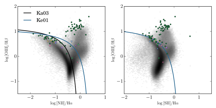
We present in figure 14 a BPT diagram for the emission line ratios: $\mathrm{[NII]/H\alpha}$, $\mathrm{[SII]/H\alpha}$, and $\mathrm{[OIII]/H\beta}$. We show typical galaxies from the MPA-JHU catalogue in grey, on a logarithmic colour scale. For our outlying galaxies, we measure the emission lines $\mathrm{[SII]}$, $\mathrm{[NII]}$, $\mathrm{H\alpha}$, $\mathrm{H\beta}$, and $\mathrm{[OIII]}$ by integration over Gaussians profiles that we fit: the $\mathrm{H\alpha}$, $\mathrm{[NII]}$ and $\mathrm{[SII]}$ are modelled jointly with 5 Gaussians at fixed rest-frame wavelengths and the $\mathrm{[OIII]}$ and $\mathrm{H\beta}$ profiles are similarly measured with 3 Gaussians. We examine the goodness of the fit by-eye, and when needed we add additional Gaussian component (e.g., if a profile is not symmetric) or allow the rest-frame wavelength to shift. We mark the emission line ratios of our outliers in green.

Kewley, Jansen & Geller (2005) analysed the effect of a fixed aperture size on metallicity, star formation rate, and reddening and concluded that a minimum aperture covering a fraction of $\approx 20$ precent is required for the spectral properties to approximate the global values, which translates to a lower limit on redshift of $z>0.04$ (for the SDSS spectrograph). Out of the 156 emission line galaxies with unusual ratios, only 86 satisfy this criterion. One can see that the outlier galaxies show emission line ratios that reside on the tails of the distribution of the entire population, which explains their weirdness score.

15 outliers are classified as HII regions with one diagnostic and AGN with another diagnostic. We show in figure 14 examples for such cases. We use two separating criteria: Kewley et al. (2001) who used a combination of population synthesis models and photoionisation models to produce a theoretical upper limit that separates between starbursts and AGN-dominated galaxies (Ke01; blue line), Kauffmann et al. (2003b) modified this limit by including composite galaxies which contain significant contribution from both star formation and AGN (Ka03; black line). Individual objects that show this duality are marked with the same colour and symbol in the two panels, for convenience. We list the 156 BPT outliers in table 7.

4.4.2 Weak $\mathrm{H\alpha}$ emission

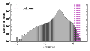
We identify 30 galaxies with emission in $\mathrm{H\alpha}$, $\mathrm{[NII]}$, and $\mathrm{[SII]}$ but none in $\mathrm{H\beta}$ and $\mathrm{[OIII]}$. Therefore, in order to study their gas emission properties, we fit and subtract a stellar population synthesis model obtained (as in section 4.1.1). These galaxies have unusually large $\mathrm{[NII]}$ and $\mathrm{S[II]}$ over $\mathrm{H\alpha}$ ratios ($\mathrm{log\,[SII]/H\alpha}\approx 0.1$). Some of the objects are low redshift galaxies, with an angular size a few times the diameter of the SDSS fibre, so the spectrum only samples a small fraction of the gas near the galactic centre.

However, we find 7 objects with $z>0.065$ and by comparison of their Petrosian radius (from SDSS photometry) to the fibre diameter we verify that the SDSS fibre indeed captures 20 percent or more of the galactic light. We measure the $\mathrm{log\,[SII]/H\alpha}$ line ratio for our objects and present it in figure 15 compared to the line ratio histogram of the MPA-JHU catalogue of galaxies from the SDSS (left panel), where one can see that our objects reside on the tail of this distribution. We give an example of such a galaxy at redshift $z=0.138$ for which $\mathrm{log\,[SII]/H\alpha}=0.17$ (right panel). We list these galaxies in table 8.

High $\mathrm{log\,[SII]/H\alpha}$ and $\mathrm{log\,[NII]/H\alpha}$ emission line ratios are generally attributed to LINER galaxies (see for example Kewley et al. 2006 and references within), though the ratios we measure for our outlier galaxies deviate from the typical ratio produced by a LINER galaxy. These galaxies can therefore be extreme cases of LINER galaxies in which we do not detect the $\mathrm{H\beta}$ and $\mathrm{[OIII]}$ emission due to limited SNR, or high dust extinction along the line of sight to the AGN. Alternatively, the high emission line ratio can be due to shock ionisation from galactic-scale winds (Heckman 1980; Dopita & Sutherland 1995; Lípari et al. 2004; Veilleux, Cecil & Bland-Hawthorn 2005; Allen et al. 2008). One can find in the literature additional examples of high $\mathrm{log\,[SII]/H\alpha}$ emission line ratios measured with integral field spectroscopy within individual lines of sight in galaxies (e.g. Singh et al. 2013 and Cheung et al. 2016).

Figure 16: Histogram of NaID excess index (see section 4.5.1 for definition) of the NaID excess objects studied by JE13 (grey bars), these are the 1603 galaxies which have the most extreme discrepancy between the observed NaID and the NaID predicted from a standard model of a galaxy. We mark the indices of the 13 outlying objects our algorithms finds, which are also present in the JE13 sample. The right panel presents the galaxy SDSS J123308.44+262057.6 (2235-53847-0086), which is not included in the JE13 catalogue, at redshift $z=0.024$ (black), compared to the SDSS best fitting model (green). One can see that the observed NaID absorption is more than double what is expected from to the best fitting model.

4.5 Extremely red and sodium excess galaxies

We find 47 galaxies that have extremely red continua and/or unusually strong sodium absorption.

4.5.1 Sodium excess galaxies

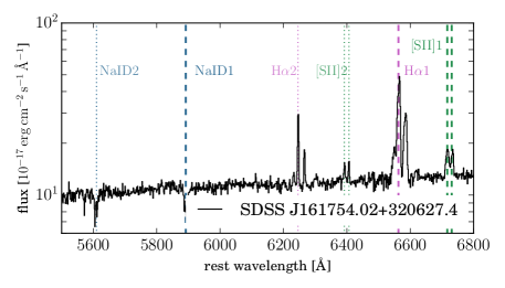
38 galaxies have very strong sodium (NaID 5889, 5895Å) absorption, some with extremely red continua as well. There is some debate in the literature regarding the origin of the NaID excess objects – one explanation is that the NaID excess is related to the interstellar medium (ISM), either due to galactic-scale gaseous outflows in star forming galaxies or cool gas that resides in the disk, another explanation is that the absorption is stellar, and due to variations in metal abundance. van Dokkum & Conroy (2010, and references therein) suggested that an initial mass function (IMF) in early-type galaxies with a larger number of low-mass stars (less than 0.3 M_⊙) may lead to stronger NaID absorption.

In order to address these questions, Jeong et al. (2013, hereafter JE13) compiled a catalogue of roughly 1000 NaID excess objects up to SDSS DR7. They limited themselves to the redshift range $z\leq 0.08$ and applied further colour cuts to ensure the completeness of their sample, from which they identified the NaID excess objects. The authors used the absorption line measurements of all the galaxies in the SDSS performed by Oh et al. (2011) and defined the index $fNaD$ as follows:

$${fNaD=\frac{NaD_{observed}-NaD_{model}}{NaD_{model}}}$$ (1)

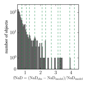
where $NaD_{observed}$ is the observed Na D line strength and $NaD_{model}$ is the expected model Na D line strength. The expected $NaD_{model}$ is also taken from Oh et al. (2011), where the authors fitted population synthesis models from Bruzual & Charlot (2003) and stellar templates by Sánchez-Blázquez et al. (2006)), and calculated internal reddening due to dust. JE13 chose 1603 galaxies for which $fNaD>0.5$ (i.e., observed strength is 50% stronger than expected by model; see figure 1 in JE13) and defined them as their sodium excess objects.

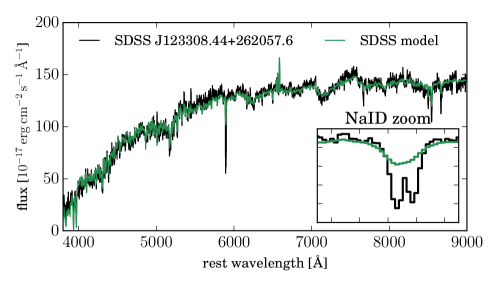
We find 24 galaxies that were not part of the JE13 sample, some for obvious reasons such as the redshift cut, the SDSS data release, and the colour cuts they performed. We find 4 galaxies which satisfy the JE13 cuts in DR7 but were not part of their sample, possibly due to erroneous measurement of the observed Na D. We present in the left panel of figure 16 the histogram of the NaID excess objects from JE13 compared to the outlying galaxies we find. In the right panel of figure 16 we show an example of such outlying galaxy, at redshift $z=0.024$, compared to the best SDSS model of this galaxy. One can see that the observed NaID is more than double the strength expected from the model. We list the NaID excess objects in table 9.

4.5.2 Extremely red galaxies

We find 19 galaxies which are extremely red, most of them show a diagonally-shaped continuum. We use the galaxy composite catalogue by Dobos et al. (2012) (hereafter DO12). DO12 classified all the galaxies in SDSS DR7 by colour, nuclear activity, and star formation activity and constructed a set of spectra with high SNR and high resolution. They fitted the continuum of the composite spectra using the population synthesis models by Bruzual & Charlot (2003) and found that the composite spectra represent the different galaxy populations well. Using the best stelar population synthesis model, they extracted the best metallically and the optical depth of interstellar dust. The DO12 composites are divided into colours – red, green, and blue – and into classes – passive, star forming, $\mathrm{H\alpha}$ detected, AGN and $\mathrm{H\alpha}$ detected (for objects which show both nuclear activity and substantial star formation), LINERs, and Seyfert galaxies.

Figure 17: Examples of two galaxies which show diagonally-shaped continua. We fit the galaxies with the galaxy composites constructed by DO12 with additional reddening in order to match their red colours. SDSS J024721.99-043259.1 (7054-56575-500; left panel; black) is best reproduced with a ‘$\mathrm{H\alpha}$ detected’ composite with total dust reddening of $\mathrm{E}_{B-V}=1.1$ (pink) and SDSS J024639.41-080525.9 (7057-56593-115; right panel; black) is best reproduced with a LINER composite with total $\mathrm{E}_{B-V}=0.98$.

Composite spectra which belong to the same class of galaxies (passive for example) but in a different colour bin differ not only in dust optical depth but also in metallicity and stellar population. We therefore use all the DO12 composite spectra and apply additional dust reddening to them in order to reach the continuum shape we observe in our galaxies. We use the prescription by Fitzpatrick (1999) for the additional dust extinction and find the best composite spectrum and the additional dust reddening to be applied to this composite in order to reproduce the continuum shape of our galaxies. We find that for all of our objects the reddest composite spectrum is a better fit than the green and the blue. For these DO12 derive metallicity value of $Z=0.02$.

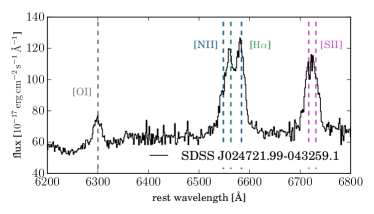
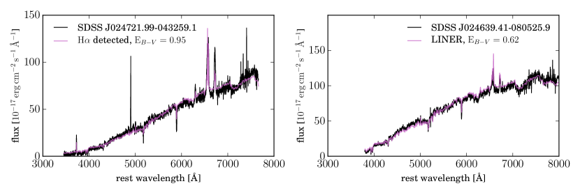
The dust reddening we find ranges from $\mathrm{E}_{B-V}=0.3$ to $\mathrm{E}_{B-V}=0.9$ for our outlying galaxies, this is in addition to the dust that is derived by DO12 in their stellar population synthesis models, giving in total colour excesses between $\mathrm{E}_{B-V}$ = $0.5$ and $2.2$. We show two examples of extremely red galaxies and their best DO12 composite plus additional reddening in figure 17. We find that the best fitting composite for SDSS J024721.99-043259.1 (7054-56575-500; left panel) belongs to the $\mathrm{H\alpha}$ detected class, with colour excess derived from population synthesis of $\mathrm{E}_{B-V}=0.15$ but with an additional $\mathrm{E}_{B-V}=0.95$. The second object (right panel), SDSS J024639.41-080525.9 (7057-56593-0115), is best described by a LINER galaxy composite with a total of $\mathrm{E}_{B-V}=0.98$. We list these galaxies in table 10, where we note specifically the galaxy SDSS J044023.25+245402.0 (1257-52944-314) with $\mathrm{E}_{B-V}=1.6$, caused by MW dust. These galaxies are rare in SDSS due to colour selection.

4.6 Galaxies hosting supernovae

We find 18 galaxies in which a supernova happens to have exploded when the spectrum was taken. Supernova rates are of order one per galaxy per century (e.g., Li et al. 2011), or one per 5000 weeks. Assuming a supernova maintains a luminosity comparable to its host’s for about a week, there should be hundreds of such objects in the SDSS galaxy sample, which is rare but not ridiculously so. There are several studies whose main goal is the detection of supernovae in the galaxy spectra of the SDSS, and they found 15 of our objects. In all of these studies, the galaxy spectra are fitted with galaxy eigenspectra that are obtained from PCA analysis of SDSS galaxies. supernovae detection is then carried out on the residual between the galaxy spectrum and its best eigenspectra fit, using various methods of template fitting: Madgwick et al. (2003) used wavelet transform in order to obtain a residual which is noiseless, and then cross-correlated it with a set of type Ia spectral templates. Tu et al. (2010); Krughoff et al. (2011); Graur & Maoz (2013); Graur, Bianco & Modjaz (2015) used PCA or singular value decomposition (SVD) of supernovae spectroscopic templates to fit the residual. In all of these cases, it was necessary to use both galaxy and supernovae templates in order to detect the supernovae. We list the outlying galaxies with supernovae in table 11.

Figure 18: SDSS J080821.09+005035.3 (4745-55892-0018) spectrum and its best SDSS model (left panel), where one can see that the SDSS model fails to account for some broad features in the spectrum. We subtract the model from the spectrum and normalise it with a continuum fit (right panel; black) and compare it to a supernova template (2 days after the peak) which we also normalise (green). One can see that the supernova template is able to account for the residual broad features in the galaxy spectrum.

SDSS J080821.09+005035.3 (4745-55892-0018) is reported here for the first time since the galaxy is part of DR10, while Graur, Bianco & Modjaz (2015) worked with the DR9 galaxy sample. We present in figure 18 the galaxy spectrum and its best SDSS model (left panel) where one can notice additional, broad, features that the best SDSS model does not account for. We subtract the best fitting SDSS model from the spectrum and normalise the residual with a continuum fit and compare the residual to a type Ia supernova template from Nugent, Kim & Perlmutter (2002) 2 days after $B$-band maximum. This is shown in the right panel of figure 18. One can see that the supernova template matches well the broad residual features in our galaxy.

SDSS J085425.56+180507.0 (2281-53711-0149) and SDSS J085436.69+180552.9 (2281-53711-0156) are also reported here for the first time. These spectra were in DR7, but the SDSS pipeline failed to fit the correct redshift to them, mistaking the $\mathrm{H\alpha}$ emission for $\mathrm{Ly\alpha}$ at high redshift. We derive the correct redshift by fitting the narrow $\mathrm{[OIII]}$ and $\mathrm{H\alpha}$ emission lines, finding redshifts of 0.094 and 0.211 respectively. For this reason they were missed by Graur, Bianco & Modjaz (2015). Using the same fitting procedure as described in Graur & Maoz (2013) and Graur, Bianco & Modjaz (2015), we find that SDSS J085425.56+180507.0 is either a type Ia or a type Ic near maximum light. SDSS J085436.69+180552.9 is most likely a type Ia near peak (O. Graur, private communication).

4.7 Blends

We find 27 outliers which are blends of two objects. These include 6 galaxy-galaxy gravitational lenses, 9 spectra with two sets of emission lines, and 12 spectra which appear unusual due to chance alignment of a galaxy and a nearby star. We list the galaxies which are contaminated by nearby stars in table 12.

Multiple studies were carried out with the goal of finding gravitationally lensed galaxies in the SDSS spectroscopic data (Bolton et al. 2004, 2005, 2006, 2008; Brownstein et al. 2012; Tsalmantza & Hogg 2012; Shu et al. 2016). These studies focused on galaxies with two sets of nebular emission lines at redshifts that differ significantly. For example, Bolton et al. (2004) used the best fitting model obtained by the SDSS pipeline and subtracted it from the spectrum, resulting in a residual spectrum. The residual spectrum underwent a match-filtering algorithm that was designed to find an additional set of emission lines. Tsalmantza & Hogg (2012) used a data-driven model which recovered most of the known galaxy lenses in the SDSS by constructing basis functions for dimensionality reduction. Overall, up to DR12, these studies have found 392 galaxy lens candidates in the SDSS. We list the six galaxy lenses our algorithm recovers in table 13, all of which were reported by previous studies.

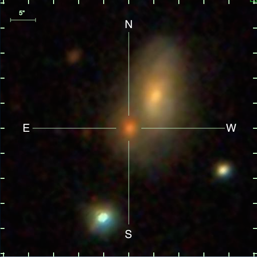
The second subset consists of objects with two sets of emission lines that were not previously reported as galaxy lenses. The second set of nebular emission lines is due to a close companion (i.e., at a small angular separation) to the primary galaxy, and in most of the objects the primary and the companion galaxy are somewhat to well distinguished in the SDSS imaging. For each of the objects, we fit two sets of emission lines with Gaussians in order to ascertain that all the nebular lines of the secondary set differ by the same velocity compared to the primary set of lines and measure the redshift of the secondary object. In all of the cases, the redshift produced by the SDSS pipeline belongs to the more luminous set of emission lines. We find that for 7 out of 8 of the objects the secondary set of emission lines is emitted by gas at a lower redshift than the primary. For three of the pairs we find an SDSS spectrum of the secondary galaxy as well as the primary, and find that the redshift estimation of the secondary galaxy is equal to the redshift we derive from the second set of emission lines in the primary’s object spectrum. We present an example of such galaxy in figure 19, where we show the SDSS image of the primary and secondary galaxy (left panel; the cross indicates the primary object) and the spectrum of the primary, shifted to its rest-frame, where one can see two sets of emission lines. The first set of emission lines is at $z=0.117$ and the second set at $z=0.063$, which is the redshift of the secondary galaxy.

Figure 19: Example of a galaxy with two sets of emission lines. The primary galaxy (SDSS J161754.02+320627.4; 1420-53146-528), marked with a cross in the image from the SDSS (left panel), is at redshift $z=0.117$. The secondary galaxy (SDSS J161753.62+320633.8) is at redshift $z=0.063$ and the gas in its outskirts is along the line of sight towards the primary galaxy. The spectrum of the primary galaxy (right panel) consists of two sets of emission lines, one at redshift $z=0.117$ and the second at redshift $z=0.063$.

We list all the objects in table 14, and note the redshift of the primary and secondary sets of lines. One of the objects, SDSS J160818.74-002745.4 (345-51690-229), is an exception since no clear companion can be seen in the imaging. Furthermore, the secondary set of emission lines is at a higher redshift than the primary galaxy, and these two sets are separated only by $2860\,\mathrm{km\,s^{-1}}$. The spectrum provided by the SDSS is a median spectrum which consists of a few sub-exposures of the same galaxy, each of them undergoes a separate wavelength solution, sky subtraction, and flux calibration. The calibrated spectra are then combined using a median filter. A wrong wavelength solution could cause the median spectrum (with which we work) to appear as a spectrum with two (or more) sets of emission lines. We compare the sub-exposures of J160818.74-002745.4 and find two sets of emission lines in all of them, indicating that this is not an instrumental error.

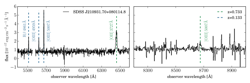
We note an additional object, SDSS J210931.70+080114.8 (4079-55363-773), for which the secondary redshift estimation is based only on two emission lines, one of which is marginally detected. The primary redshift of the galaxy is $z=0.133$ and no clear companion is detected in the imaging. However, we find an unidentified emission line in wavelength 6460 Å  in the observer’s frame, and its FWHM is inconsistent with the FWHM of the emission lines of the galaxy. Assuming the unidentified emission line is due to $\mathrm{[OII]}$ 3727 Å  in the rest-frame of a background galaxy, we estimate the redshift of the background galaxy to be $z=0.733$. We show the spectrum of the galaxy in figure 20, where the supposedly $\mathrm{[OII]}$ emission is marked with a green dashed line (left panel). In the right panel of figure 20 we mark the wavelength of $\mathrm{[OIII]}$ 5007 Å  in the observers frame for the redshift $z=0.733$, which match a weak feature in the spectrum. The FWHM values of both of them are consistent with each other. The flux of the $\mathrm{[OII]}$ emission is in the range expected from star forming galaxies at redshift $z=0.733$, thus no magnification is needed in order to explain the $\mathrm{[OII]}$ emission strength. We therefore conclude that their background galaxy is not strongly lensed.

4.8 Calibration errors, source confusion and sky contamination

This group of outliers is a mixed bag of objects that are broadly defined as not being astronomically ‘interesting’. This includes calibration errors and SDSS pipeline misclassifications. In section 2 we remove pixels that are marked as bad by the SDSS pipeline, and we also apply a median filter for the removal of residual cosmic rays and unresolved sky emission. The SDSS also provide quality flags for all the plates and all their spectra. Since we do not limit ourselves to plates of good quality only, it is inevitable that some bad spectra exist in our dataset. Additionally, our algorithm finds the relatively few objects that were misclassified by the SDSS pipeline, and we include them here.

First, we identify 41 galaxy spectra that are in fact single stars. Additionally, we find 5 spectra of white dwarfs that were mistakenly identified as galaxies, 4 of these were previously reported as white dwarfs by Girven et al. (2011) and Kleinman et al. (2013), and one of them, SDSS J103259.82+442202.2 (2567-54179-177), is reported here for the first time. SDSS J141118.31+481257.6 (1671-53446-0010) is identified as a galaxy at redshift 0.135 by the SDSS pipeline. However, it is actually an AM Canum Venaticorum star, which is a rare type of cataclysmic variable star, where a white dwarf accretes hydrogen-poor matter from a compact companion star (Anderson et al. 2005). We list these in table 15. Finally, 10 objects suffer from various problems such as bad sky subtraction, and wrong flux calibration (i.e., flux level from the blue and red arms of the spectrograph do not match; table 16).

Figure 20: SDSS J210931.70+080114.8 (4079-55363-773) is a galaxy at redshift $z=0.133$ for which we detect an emission line in wavelength 6460 Å  in the observers frame. This emission line is broader than the emission lines that belong to this galaxy (left panel) and does not match in wavelength to any known emission lines at redshift $z=0.133$. Assuming the emission line is due to $\mathrm{[OII]}$ 3727 Å  in the rest-frame of a background galaxy, we estimate the redshift of the background galaxy to be $z=0.733$. We mark in the right panel the wavelength of $\mathrm{[OIII]}$ 5007 Å  in the observers frame for the redshift $z=0.733$, which matches a weak feature in the spectrum. Since the flux of the supposed $\mathrm{[OII]}$ emission is within the range expected for galaxies at redshift $z=0.7$, we conclude that this galaxy is another case of galaxy-galaxy chance alignment.

5 Conclusions and Discussion

We have introduced an outlier detection algorithm that is based on an unsupervised implementation of RF. By construction, the algorithm learns the most important features of the data and their interconnections; it is completely general and can be applied to imaging data, time-series, and other spectroscopic objects as well. Out of 2 355 926 galaxies which compose the input sample, we chose 400 galaxies with the highest weirdness score. We find objects with unusual emission line ratios, and complex velocity structures, extremely red objects, objects with extremely strong absorption lines (i.e. sodium and $\mathrm{H\delta}$), galaxies which host supernovae, or have rare emission lines.

The algorithm finds a large variety of outliers arising from a large variety of physical environments. It is sensitive to the ratio between emission lines, thus to the radiation field that gas in a galaxy is exposed to, and to the metallically of the gas. It is sensitive to the widths of emission lines i.e., objects with extreme velocity dispersion, or with a number of different velocity components. It is sensitive to the shape of the continuum and to its connection to the strength of the emission lines and absorption lines. It recovers a number of rare phenomena that are subject to great attention in the astronomical community: $\mathrm{H\delta}$-strong galaxies, outflows and shocks, supernovae, galaxy-lenses, double-peaked emission lines which may be due to galaxy mergers or binary BHs. Only about a fifth of the objects we find were discovered in previous studies, using specific algorithms that isolate a single type of objects they were looking for (or searching by eye). Our algorithm detects all of them in one fell swoop. Despite how thoroughly SDSS has been explored before, we found two rare classes of galaxies that were never noticed or studied before, E+A galaxies with broad emission lines, and strong-$\mathrm{[NI]}$ emitting galaxies.

Apart from these, the algorithm detects a number of different ‘instrumental’ outliers, and can be used to detect pipeline failures in new or ongoing surveys. Most importantly, since the sole input to the algorithm is the data, with no physical rules or user specifications, and we find that it is able to detect some of the most interesting phenomena in the SDSS sample, this algorithm can be used to search for new objects that represent new phenomena – searching for the truly unknown unknowns.

From a performance perspective, the increasing volume and complexity of astronomical data requires the development of new algorithms for detection, classification, and analysis of large datasets. The The Large Synoptic Survey Telescope (LSST) for example, is expected to conduct 32 trillion observations of 40 billion objects (Ivezic et al. 2008). These datasets can no longer be placed on a single compute node nor can they be analysed at once with a single processor. The framework of DFS has evolved as a possible solution to this challenge and parallelisation had become an essential methodology in it. The RF-based outlier detection we propose is completely parallel and operates naturally in the DFS framework. Furthermore, the algorithm is suitable for ongoing surveys where static data is replaced by data streams – new data is chunked and decision trees are trained without the need to re-run the process on the entire dataset. RF’s ability to operate with missing values is an additional important feature. Finally, the algorithm can work with an extremely large number of features with little to no cost in execution time.

Appendix A Outlying galaxies – summary

We summarise all the galaxies we present in the paper in the next tables. We note that some galaxies are classified into multiple categories, in this case we present the galaxy in every class (and table) it belongs to.

Table 1: Unusual velocity structure

PLATE	MJD	FIBER	z	References
(1)	(2)	(3)	(4)	(5)
1323	52797	335	0.116
2117	54115	230	0.113
3788	55246	275	0.475
4767	55946	889	0.499	SC13
7163	56593	697	0.599
(1) – SDSS plate ID of the galaxy.
(2) – SDSS MJD of the observation.
(3) – SDSS fiber ID of the galaxy.
(4) – Redshift from SDSS pipeline, whenever available we use $z_{NOQSO}$ which is more reliable.
(5) – Previous studies of the galaxy, if exist: SC13 – Schirmer et al. (2013)

Table 2: Galaxies with additional velocity structure near $\mathrm{H\alpha}$

PLATE	MJD	FIBER	z	Comments
(1)	(2)	(3)	(4)	(5)
663	52145	306	0.041
1222	52763	341	0.028
1330	52822	391	0.111
1377	53050	441	0.009
1453	53084	289	4.5	$z=0.038$
1724	53859	116	0.037
2022	53827	286	0.023
2511	53882	29	0.172
2660	54504	446	0.016
3929	55335	835	0.184
6138	56598	213	0.248
(1) – SDSS plate ID of the galaxy.
(2) – SDSS MJD of the observation.
(3) – SDSS fiber ID of the galaxy.
(4) – Redshift from SDSS pipeline, whenever available we use $z_{NOQSO}$ which is more reliable.
(5) – Additional comments, if the redshift given by the SDSS pipeline is wrong we note the correct redshift.

Table 3: Double-peaked emission-line galaxies

PLATE	MJD	FIBER	z	Comments	References
(1)	(2)	(3)	(4)	(5)	(6)
397	51794	109	0.018
1360	53033	186	0.19		GE12, PI12
1566	53003	429	0.246
2266	53679	422	0.016
4391	55866	835	0.069
4755	55660	45	0.433
5049	56103	273	0.229	$z=0.608$
5867	56034	304	0.15		XU09, SM10
6788	56428	257	0.214	$z=0.590$
7047	56572	461	0.534
662	52147	180	5.7	broad components, $z=0.259$	ST03, WU04, ST08
733	52207	222	0.239	broad components	ST03, WU04, BI07
838	52378	460	5.1	broad components, $z=0.131$	ST03, WU04, BI07
(1) – SDSS plate ID of the galaxy.
(2) – SDSS MJD of the observation.
(3) – SDSS fiber ID of the galaxy.
(4) – Redshift from SDSS pipeline, whenever available we use $z_{NOQSO}$ which is more reliable.
(5) – Additional comments, if the redshift given by the SDSS pipeline is wrong we note the correct redshift.
(6) – Previous studies of the galaxy, if exist: ST03 – Strateva et al. (2003), WU04 – Wu & Liu (2004), BI07 – Bian et al. (2007),
ST08 – Strateva et al. (2008), XU09 – Xu & Komossa (2009), SM10 – Smith et al. (2010), GE12 – Ge et al. (2012),
PI12 – Pilyugin et al. (2012).

Table 4: Broad $\mathrm{[OIII]}$ emission line

PLATE	MJD	FIBER	z	Comments	FWHM
(1)	(2)	(3)	(4)	(5)	(6)
2089	53498	416	0.081		930
2357	53793	115	0.109		830
3859	55246	651	0.177	$z=0.54317$	620
4295	55858	929	0.198		710
4776	55652	25	0.217	$z=0.59778$	790
5129	55864	169	0.185		1000
6031	56091	7	0.246	$z=0.63461$	930
6402	56334	838	0.153	$z=0.5125$	1030
6465	56279	757	0.08		950
6592	56535	653	0.18		690
6974	56442	627	0.506		880
7101	56659	293	0.088		780
6473	56363	672	0.116		610
(1) – SDSS plate ID of the galaxy.
(2) – SDSS MJD of the observation.
(3) – SDSS fiber ID of the galaxy.
(4) – Redshift from SDSS pipeline, whenever available we use $z_{NOQSO}$ which is more reliable.
(5) – Additional comments, if the redshift given by the SDSS pipeline is wrong we note the correct redshift.
(6) – Full width at half maximum of the $\mathrm{[OIII]}$ emission line in $\mathrm{km\,s^{-1}}$.

Table 5: $\mathrm{H\delta}$ strong galaxies

PLATE	MJD	FIBER	z	Comments	References
(1)	(2)	(3)	(4)	(5)	(6)
403	51871	219	0.156		GO03
457	51901	166	0.116		GO03
538	52029	413	0.264		GO03, GO04, BA05, GO07, ME13
611	52055	128	0.130		GO03
629	52051	561	0.154		GO03, BA05
719	52203	555	0.157	broad emission
781	52373	607	0.167		GO07, ME13
819	52409	369	0.136		GO07
870	52325	536	0.143		GO07, ME13
1185	52642	345	0.296		GO07, ME13
1223	52781	386	0.004
1311	52765	359	0.163		GO07, ME13
1366	53063	430	0.182		GO07, ME13
1429	52990	416	0.17		GO07, ME13
1463	53063	262	0.125	broad emission
1574	53476	577	0.192		GO07, ME13
1578	53496	1	0.173		GO07
1583	52941	333	0.273		GO07, ME13
1616	53169	135	0.008
1621	53383	336	0.185		ME13
1658	53240	319	0.123		GO07, ME13
1701	53142	496	0.28
1769	53502	17	0.228		ME13
1989	53772	606	0.127		ME13
2022	53827	88	0.168		ME13
2123	53793	77	0.139		ME13
2165	53917	68	0.296		ME13
2168	53886	332	0.134		ME13
2225	53729	345	0.178		ME13
2292	53713	73	0.176		ME13
2608	54474	8	0.177		ME13
2789	54555	502	0.188		ME13
2791	54556	321	0.185		ME13
(1) – SDSS plate ID of the galaxy.
(2) – SDSS MJD of the observation.
(3) – SDSS fiber ID of the galaxy.
(4) – Redshift from SDSS pipeline, whenever available we use $z_{NOQSO}$ which is more reliable.
(5) – Additional comments, if the redshift given by the SDSS pipeline is wrong we note the correct redshift.
(6) – Previous studies of the galaxy, if exist: GO03 – Goto et al. (2003), GO04 – Goto (2004),
BA05 – Balogh et al. (2005), GO07 – Goto (2007), ME13 – Melnick & De Propris (2013).

Table 6: Unusual emission lines

PLATE	MJD	FIBER	z	Comments	References
(1)	(2)	(3)	(4)	(5)	(6)
2580	54092	470	0.101	coronal lines	WA12
4312	55511	732	0.059	coronal lines
6473	56363	672	0.116	coronal lines
519	52283	415	0.023	$\mathrm{[NI]}$ emission
533	51994	537	0.025	$\mathrm{[NI]}$ emission
575	52319	200	0.29	$\mathrm{[NI]}$ emission
667	52163	205	0.013	$\mathrm{[NI]}$ emission
727	52207	504	0.043	$\mathrm{[NI]}$ emission
1324	53088	456	0.005	$\mathrm{[NI]}$ emission
1388	53119	128	0.362	$\mathrm{[NI]}$ emission
1816	53919	545	0.042	$\mathrm{[NI]}$ emission
2440	53818	135	0.136	$\mathrm{[NI]}$ emission
(1) – SDSS plate ID of the galaxy.
(2) – SDSS MJD of the observation.
(3) – SDSS fiber ID of the galaxy.
(4) – Redshift from SDSS pipeline, whenever available we use $z_{NOQSO}$ which is more reliable.
(5) – Additional comments, if the redshift given by the SDSS pipeline is wrong due to broad emission lines we note the correct redshift.
(6) – Previous studies of the galaxy, if exist: WA12 – Wang et al. (2012).

Table 7: Outliers on BPT diagram

PLATE	MJD	FIBER	z	PLATE	MJD	FIBER	z	PLATE	MJD	FIBER	z
(1)	(2)	(3)	(4)	(1)	(2)	(3)	(4)	(1)	(2)	(3)	(4)
267	51608	384	0.006	1162	52668	406	0.127	2131	53819	447	0.174
280	51612	192	0.099	1198	52669	230	0.128	2167	53889	71	0.011
284	51943	170	0.005	1216	52709	619	0.016	2218	53816	133	0.141
291	51928	560	0.089	1291	52738	523	0.018	2228	53818	334	0.025
330	52370	471	0.004	1311	52765	262	0.051	2233	53845	371	0.009
336	51999	198	0.011	1311	52765	519	0.174	2238	54205	222	0.004
444	51883	199	0.017	1324	53088	183	0.001	2245	54208	467	0.047
446	51899	529	0.047	1325	52762	634	0.152	2266	53679	422	0.016
446	51899	597	0.113	1327	52781	18	0.03	2286	53700	472	0.032
450	51908	409	0.047	1333	52782	585	0.119	2297	53738	349	0.295
460	51924	616	0.034	1366	53063	83	0.019	2322	53727	365	0.026
462	51909	444	0.085	1382	53115	193	0.014	2421	54153	494	0.033
468	51912	233	0.051	1427	52996	221	0.004	2494	54174	361	0.005
486	51910	231	0.039	1451	53117	116	0.187	2497	54154	246	0.021
488	51914	555	0.122	1467	53115	579	0.067	2513	54141	309	0.027
489	51930	50	0.006	1513	53741	637	0.042	2525	54569	606	0.035
499	51988	84	0.021	1601	53115	547	0.004	2528	54571	470	0.065
516	52017	119	0.007	1602	53117	380	0.022	2561	54597	345	0.09
519	52283	124	0.026	1612	53149	73	0.021	2638	54095	614	0.067
521	52326	300	0.006	1615	53166	120	0.004	2648	54485	584	0.115
546	52205	419	0.047	1625	53140	626	0.139	2742	54233	385	0.089
553	51999	342	0.03	1626	53472	190	0.014	2748	54234	456	0.162
556	51991	11	0.005	1655	53523	526	0.014	2772	54529	566	0.116
574	52355	356	0.122	1672	53460	489	0.026	2776	54554	219	0.186
603	52056	192	0.144	1692	53473	6	0.091	2779	54540	261	0.032
616	52442	364	0.002	1701	53142	180	0.237	2880	54509	230	0.018
624	52377	361	0.002	1707	53885	587	0.277	2961	54550	550	0.176
647	52553	235	0.059	1719	53876	196	0.082	3676	55186	109	0.132
657	52177	458	0.019	1724	53859	318	0.011	3788	55246	275	0.475
735	52519	461	0.116	1740	53050	265	0.031	3942	55338	939	0.086
753	52233	94	0.014	1740	53050	295	0.12	3946	55659	189	0.146
761	54524	477	0.095	1745	53061	196	0.01	4181	55685	230	0.103
764	52238	266	0.054	1751	53377	288	0.06	4317	55480	655	0.417
778	54525	278	0.004	1761	53376	293	0.021	4320	55894	922	0.124
778	54525	497	0.04	1782	53299	412	0.1	4352	55533	227	0.133
788	52338	311	0.01	1787	54465	443	0.005	5022	55827	133	0.409
844	52378	445	0.018	1788	54468	239	0.016	5309	55929	249	0.079
853	52374	422	0.058	1802	53885	602	0.168	5357	55956	673	0.181
853	52374	577	0.08	1805	53875	413	0.15	5428	56029	869	0.15
861	52318	489	0.02	1814	54555	395	0.049	5430	56000	211	0.399
880	52367	588	0.049	1975	53734	467	0.002	5994	56101	342	0.352
896	52592	34	0.054	2001	53493	146	0.001	6000	56102	85	0.107
900	52637	534	0.192	2003	53442	450	0.04	6140	56189	595	0.073
934	52672	483	0.187	2016	53799	185	0.004	6293	56561	573	0.106
939	52636	403	0.128	2016	53799	430	0.016	6402	56334	33	0.056
939	52636	637	0.145	2016	53799	590	0.045	6415	56310	569	0.409
952	52409	247	0.01	2019	53430	327	0.1	6431	56311	161	0.064
955	52409	608	0.002	2025	53431	7	0.006	6474	56362	767	0.208
964	52646	570	0.047	2026	53711	425	0.002	6514	56487	671	0.128
1018	52672	359	0.004	2095	53474	347	0.01	6596	56331	812	0.101
1039	52707	288	0.023	2097	53491	183	0.031	7050	56573	475	0.039
1048	52736	424	0.092	2117	54115	351	0.008	7164	56597	405	0.466
(1) – SDSS plate ID of the galaxy.
(2) – SDSS MJD of the observation.
(3) – SDSS fiber ID of the galaxy.
(4) – Redshift from SDSS pipeline, whenever available we use $z_{NOQSO}$ which is more reliable.

Table 8: Weak $\mathrm{H\alpha}$ emission

PLATE	MJD	FIBER	z	$\mathrm{log\,[SII]/H\alpha}$	$\mathrm{log\,[NII]/H\alpha}$
(1)	(2)	(3)	(4)	(5)	(6)
298	51955	204	0.012	-0.026	0.062
405	51816	603	0.021	0.007	0.161
422	51878	80	0.094	0.117	0.027
447	51877	376	0.059	-0.181	0.218
468	51912	523	0.035	-0.022	0.156
519	52283	415	0.023	0.200	0.230
533	51994	537	0.025	0.088	0.055
667	52163	205	0.013	-0.014	0.021
727	52207	504	0.043	0.047	-0.141
1251	52964	559	0.059	0.120	0.190
1324	53088	456	0.005	0.130	0.214
1327	52781	215	0.007	0.002	-0.142
1404	52825	251	0.048	0.019	0.007
1430	53002	356	0.023	0.183	0.286
1460	53138	244	0.028	0.076	0.220
1707	53885	113	0.12	0.060	0.050
1719	53876	89	0.034	-0.084	-0.170
1816	53919	545	0.042	0.092	0.223
2028	53818	60	0.014	0.129	0.125
2105	53472	230	0.022	0.073	0.164
2199	53556	78	0.04	0.090	0.101
2440	53818	135	0.136	0.108	0.127
2487	53852	117	0.047	0.020	0.236
4745	55892	18	0.102	0.120	0.311
5994	56101	342	0.352	0.054	0.297
6138	56598	270	0.198	0.044	0.038
6258	56238	282	0.183	0.018	0.009
6261	56219	680	0.191	0.137	0.154
7054	56575	500	0.138	0.171	0.063
7057	56593	115	0.068	0.053	-0.079
(1) – SDSS plate ID of the galaxy.
(2) – SDSS MJD of the observation.
(3) – SDSS fiber ID of the galaxy.
(4) – Redshift from SDSS pipeline, whenever available we use $z_{NOQSO}$ which is more reliable.
(5) – $\mathrm{log\,[SII]/H\alpha}$ measurement for the galaxy.
(6) – $\mathrm{log\,[NII]/H\alpha}$ measurement for the galaxy.

Table 9: Sodium excess galaxies

PLATE	MJD	FIBER	z	References
(1)	(2)	(3)	(4)	(5)
267	51608	508	0.013
411	51817	362	0.072	JE13
412	52258	180	0.127
412	52258	492	0.047	JE13
427	51900	71
440	51885	227	0.117
468	51912	523	0.035
473	51929	492	0.085	GO03, GO07, ME13
512	51992	536	0.109
588	52045	622	0.044	JE13
591	52022	467	0.037
613	52345	393	0.008
667	52163	205	0.013	JE13
676	52178	420	0.016
731	52460	381	0.029	JE13
862	52325	108	0.103
1055	52761	515	0.103
1251	52964	559	0.059
1303	53050	443	0.011	JE13
1617	53112	454	0.107
1620	53137	443	0.022
1624	53386	594	0.009
1672	53460	489	0.026	JE13
1707	53885	113	0.12
1719	53876	89	0.034
1946	53432	350	0.005
2199	53556	78	0.04	JE13
2120	53852	540	0.027	JE13
2201	53904	263	0.114
2235	53847	86	0.024
2418	53794	116	0.035
2508	53875	389	0.012	JE13
2754	54240	372	0.013	JE13
2777	54554	201	0.037	JE13
2787	54552	606	0.044	JE13
7140	56569	428	0.065
7161	56625	262	0.075
7161	56625	702	0.041
(1) – SDSS plate ID of the galaxy.
(2) – SDSS MJD of the observation.
(3) – SDSS fiber ID of the galaxy.
(4) – Redshift from SDSS pipeline, whenever available we use $z_{NOQSO}$ which is more reliable.
(5) – Previous studies of the galaxy, if exist: GO03 – Goto et al. (2003), GO07 – Goto (2007),
JE13 – Jeong et al. (2013), ME13 – Melnick & De Propris (2013).

Table 10: Extremely red galaxies

PLATE	MJD	FIBER	z	Best template	Additional reddening
(1)	(2)	(3)	(4)	(5)	(6)
591	52022	467	0.037	H$\alpha$ detected	$\mathrm{E}_{B-V}=0.64$ mag
676	52178	420	0.016	H$\alpha$ detected	$\mathrm{E}_{B-V}=0.70$ mag
1251	52964	559	0.059	LINER	$\mathrm{E}_{B-V}=0.65$ mag
1254	52972	234	0.013	H$\alpha$ detected	$\mathrm{E}_{B-V}=0.92$ mag
1257	52944	314	0.012	MW dust cloud, $\mathrm{A_{r}}=4.42$
1617	53112	454	0.107	H$\alpha$ detected	$\mathrm{E}_{B-V}=0.38$ mag
1707	53885	113	0.12	AGN + H$\alpha$	$\mathrm{E}_{B-V}=0.30$ mag
1719	53876	89	0.034	AGN + H$\alpha$	$\mathrm{E}_{B-V}=0.97$ mag
1946	53432	350	0.005	H$\alpha$ detected	$\mathrm{E}_{B-V}=0.64$ mag
2120	53852	540	0.027	H$\alpha$ detected	$\mathrm{E}_{B-V}=0.62$ mag
2418	53794	116	0.035	AGN + H$\alpha$	$\mathrm{E}_{B-V}=0.50$ mag
2508	53875	389	0.012	H$\alpha$ detected	$\mathrm{E}_{B-V}=0.84$ mag
7035	56568	452	0.1	H$\alpha$ detected	$\mathrm{E}_{B-V}=0.68$ mag
7048	56575	454	0.063	H$\alpha$ detected	$\mathrm{E}_{B-V}=0.95$ mag
7056	56577	500	0.087	AGN + H$\alpha$	$\mathrm{E}_{B-V}=0.72$ mag
7152	56660	174	0.122	Star-forming	$\mathrm{E}_{B-V}=0.70$ mag
7054	56575	500	0.138	AGN + H$\alpha$	$\mathrm{E}_{B-V}=0.83$ mag
7057	56593	115	0.068	LINER	$\mathrm{E}_{B-V}=0.63$ mag
7161	56625	262	0.075	Star-forming	$\mathrm{E}_{B-V}=0.78$ mag
(1) – SDSS plate ID of the galaxy.
(2) – SDSS MJD of the observation.
(3) – SDSS fiber ID of the galaxy.
(4) – Redshift from SDSS pipeline, whenever available we use $z_{NOQSO}$ which is more reliable.
(5) – Best fitting template from the SDSS galaxy composites by Dobos et al. (2012).
(6) – Additional dust reddening to be applied in order to obtain the continuum shape of the galaxy.

Table 11: Galaxies hosting supernovae

PLATE	MJD	FIBER	z	References	Comments
(1)	(2)	(3)	(4)	(5)	(6)
424	51893	355	0.054	GR15	Ia
438	51884	462	0.117	GR15	Ia
472	51955	247	0.07	MA03	Ia
475	51965	626	0.031	GR15	Ia
966	52642	221	0.074	GR15	Ia
1304	52993	552	0.094	GR15	Ia
1392	52822	147	0.05	GR15	Ia
1462	53112	638	0.028	GR15	Ia
1744	53055	210	0.06	GR15	Ia
2199	53556	232	0.045	GR15	Ia
2202	53566	403	0.084	GR15	Ia
2222	53799	480	0.076	GR15	Ia
2430	53815	267	0.051	GR15	Ia
2744	54272	561	0.014	GR15	Ia
2792	54556	210	0.036	GR15	Ia
2281	53711	149	4.9		$z=0.094$, Ic +4 days
2281	53711	156	4.9		$z=0.211$, Ia, +3.2 days
4745	55892	18	0.102		Ia +2 days
(1) – SDSS plate ID of the galaxy.
(2) – SDSS MJD of the observation.
(3) – SDSS fiber ID of the galaxy.
(4) – Redshift from SDSS pipeline, whenever available we use $z_{NOQSO}$ which is more reliable.
(5) – Previous studies of the galaxy, if exist: MA03 – Madgwick et al. (2003), GR15 – Graur, Bianco & Modjaz (2015).
(6) – Additional comments: supernova type, correct redshift (if necessary), supernova age (if reported for the first time).

Table 12: Chance alignment – galaxy and a nearby star

PLATE	MJD	FIBER	z
(1)	(2)	(3)	(4)
269	51910	466	0.178
691	52199	123	0.014
967	52636	302	0.001
1010	52649	301	0.022
1784	54425	75	0.085
2100	53713	106	0.024
2477	54058	460	0.044
2516	54241	391	0.035
4350	55556	266	0.205
5068	55749	474	0.161
6138	56598	559	0.189
6485	56342	655	0.023
(1) – SDSS plate ID of the galaxy.
(2) – SDSS MJD of the observation.
(3) – SDSS fiber ID of the galaxy.
(4) – Redshift from SDSS pipeline, whenever available we use $z_{NOQSO}$ which is more reliable.

Table 13: Galaxy-galaxy gravitational lenses

PLATE	MJD	FIBER	z	References
(1)	(2)	(3)	(4)	(5)
328	52282	535	0.106	BO08
393	51794	456	0.1196	BO08
499	51988	5	0.123	BO08
615	52347	594	0.1428	BO08
807	52295	614	0.2803	BO08
969	52442	134	0.215	BO08
(1) – SDSS plate ID of the galaxy.
(2) – SDSS MJD of the observation.
(3) – SDSS fiber ID of the galaxy.
(4) – Redshift from SDSS pipeline, whenever available we use $z_{NOQSO}$ which is more reliable.
(5) – Previous studies of the galaxy, if exist: BO08 – Bolton et al. (2008).

Table 14: Multiple emission-line systems

PLATE	MJD	FIBER	z	$\mathrm{z_{sec}}$
(1)	(2)	(3)	(4)	(5)
345	51690	229	0.113	0.1230
746	52238	531	0.103	0.0463
1420	53146	528	0.117	0.0627
1421	53149	253	0.133	0
1543	53738	574	0.125	0.0944
1699	53148	495	0.148	0.1069
1762	53415	435	0.13	0.0019
4079	55363	773	0.133	0.733
5399	55956	245	0.276	0.0425
(1) – SDSS plate ID of the galaxy.
(2) – SDSS MJD of the observation.
(3) – SDSS fiber ID of the galaxy.
(4) – Redshift from SDSS pipeline, whenever available we use $z_{NOQSO}$ which is more reliable.
(5) – Redshift of the second set of emission lines.

Table 15: Stars identified as galaxies

PLATE	MJD	FIBER	Comments	References
(1)	(2)	(3)	(4)	(5)
465	51910	482
550	51959	433
1237	52762	621
1246	54478	520
1247	52677	229
1247	52677	229
1247	52677	259
1250	52930	543
1251	52964	193
1256	52902	585
1256	52902	402
1256	52902	506
1256	52902	362
1256	52902	38
1256	52902	636
1257	52944	253
1257	52944	300
1257	52944	209
1257	52944	244
1642	53115	81
1999	53503	224
2266	53679	82
2445	54573	16
2538	54271	381
2538	54271	261
2538	54271	359
2538	54271	59
2546	54625	124
2555	54265	8
2555	54265	10
2568	54153	3
2714	54208	222
2799	54368	3
2806	54425	5
2807	54433	195
2815	54414	228
3175	54828	372
3290	54941	314
3324	54943	272
3480	54999	228
5042	55856	436
550	51959	433	WD	GI11
1237	52762	621	WD	KL13
1679	53149	616	WD	KL13
1702	53144	178	WD	KL13
2567	54179	177	WD
1671	53446	10	AM CVn	AN05
(1) – SDSS plate ID of the galaxy.
(2) – SDSS MJD of the observation.
(3) – SDSS fiber ID of the galaxy.
(4) – Additional comments.
(5) – Previous studies, if exist: AN05 – Anderson et al. (2005), GI11 – Girven et al. (2011), KL13 – Kleinman et al. (2013).

Table 16: Bad spectra

PLATE	MJD	FIBER	z	Comments
(1)	(2)	(3)	(4)	(5)
434	51885	639	0.073	sky subtraction
446	51899	139	0.754	redshift estimation
468	51912	233	0.051	sky subtraction
473	51929	374	0.271	flux calibration
767	52252	313	0.014	flux calibration
1019	52707	261	0.008	H$\alpha$ emission is cut off
1360	53003	633	0.124	sky emission
1809	53792	99	0.058	H$\alpha$ emission is cut off
2134	53876	45	0.053	H$\alpha$ emission is cut off
5001	55719	40	0.201	flux calibration
(1) – SDSS plate ID of the galaxy.
(2) – SDSS MJD of the observation.
(3) – SDSS fiber ID of the galaxy.
(4) – Redshift from SDSS pipeline, whenever available we use $z_{NOQSO}$ which is more reliable.
(5) – Description of the source of contamination.

References

- Ahn et al. (2012) Ahn C. P. et al., 2012, ApJS, 203, 21
- Alam et al. (2015) Alam S. et al., 2015, ApJS, 219, 12
- Alatalo et al. (2016) Alatalo K. et al., 2016, ApJS, 224, 38
- Alexander et al. (2010) Alexander D. M., Swinbank A. M., Smail I., McDermid R., Nesvadba N. P. H., 2010, in Astronomical Society of the Pacific Conference Series, Vol. 427, Accretion and Ejection in AGN: a Global View, Maraschi L., Ghisellini G., Della Ceca R., Tavecchio F., eds., p. 74
- Allen et al. (2008) Allen M. G., Groves B. A., Dopita M. A., Sutherland R. S., Kewley L. J., 2008, ApJS, 178, 20
- Anderson et al. (2005) Anderson S. F. et al., 2005, AJ, 130, 2230
- Andrae, Melchior & Bartelmann (2010) Andrae R., Melchior P., Bartelmann M., 2010, A&A, 522, A21
- Ascasibar & Sánchez Almeida (2011) Ascasibar Y., Sánchez Almeida J., 2011, MNRAS, 415, 2417
- Bailey (2012) Bailey S., 2012, PASP, 124, 1015
- Baker et al. (2015) Baker P. T., Caudill S., Hodge K. A., Talukder D., Capano C., Cornish N. J., 2015, Phys. Rev. D, 91, 062004
- Baldwin, Phillips & Terlevich (1981) Baldwin J. A., Phillips M. M., Terlevich R., 1981, PASP, 93, 5
- Ball & Brunner (2010) Ball N. M., Brunner R. J., 2010, International Journal of Modern Physics D, 19, 1049
- Balogh et al. (2005) Balogh M. L., Miller C., Nichol R., Zabludoff A., Goto T., 2005, MNRAS, 360, 587
- Baron et al. (2015) Baron D., Poznanski D., Watson D., Yao Y., Cox N. L. J., Prochaska J. X., 2015, MNRAS, 451, 332
- Bellm (2014) Bellm E., 2014, in The Third Hot-wiring the Transient Universe Workshop, Wozniak P. R., Graham M. J., Mahabal A. A., Seaman R., eds., pp. 27–33
- Bian et al. (2007) Bian W.-H., Chen Y.-M., Gu Q.-S., Wang J.-M., 2007, ApJ, 668, 721
- Bloom et al. (2012) Bloom J. S. et al., 2012, PASP, 124, 1175
- Bolton et al. (2008) Bolton A. S., Burles S., Koopmans L. V. E., Treu T., Gavazzi R., Moustakas L. A., Wayth R., Schlegel D. J., 2008, ApJ, 682, 964
- Bolton et al. (2005) Bolton A. S., Burles S., Koopmans L. V. E., Treu T., Moustakas L. A., 2005, ApJ, 624, L21
- Bolton et al. (2006) Bolton A. S., Burles S., Koopmans L. V. E., Treu T., Moustakas L. A., 2006, ApJ, 638, 703
- Bolton et al. (2004) Bolton A. S., Burles S., Schlegel D. J., Eisenstein D. J., Brinkmann J., 2004, AJ, 127, 1860
- Bolton et al. (2012) Bolton A. S. et al., 2012, AJ, 144, 144
- Breiman (2001) Breiman L., 2001, Machine Learning, 45, 5
- Breiman et al. (1984) Breiman L., Friedman J. H., Olshen R. A., Stone C. J., 1984, Monterey, CA: Wadsworth & Brooks/Cole Advanced Books & Software
- Brinchmann et al. (2004) Brinchmann J., Charlot S., White S. D. M., Tremonti C., Kauffmann G., Heckman T., Brinkmann J., 2004, MNRAS, 351, 1151
- Brownstein et al. (2012) Brownstein J. R. et al., 2012, ApJ, 744, 41
- Bruzual & Charlot (2003) Bruzual G., Charlot S., 2003, MNRAS, 344, 1000
- Cappellari (2012) Cappellari M., 2012, pPXF: Penalized Pixel-Fitting stellar kinematics extraction. Astrophysics Source Code Library
- Cappellari & Emsellem (2004) Cappellari M., Emsellem E., 2004, PASP, 116, 138
- Carniani et al. (2015) Carniani S. et al., 2015, A&A, 580, A102
- Cheung et al. (2016) Cheung E. et al., 2016, Nature, 533, 504
- Collister & Lahav (2004) Collister A. A., Lahav O., 2004, PASP, 116, 345
- Costero & Osterbrock (1977) Costero R., Osterbrock D. E., 1977, ApJ, 211, 675
- Daniel et al. (2011) Daniel S. F., Connolly A., Schneider J., Vanderplas J., Xiong L., 2011, AJ, 142, 203
- Djorgovski et al. (2016) Djorgovski S. G., Graham M. J., Donalek C., Mahabal A. A., Drake A. J., Turmon M., Fuchs T., 2016, ArXiv e-prints: 1601.04385
- Dobos et al. (2012) Dobos L., Csabai I., Yip C.-W., Budavári T., Wild V., Szalay A. S., 2012, MNRAS, 420, 1217
- Dopita & Sutherland (1995) Dopita M. A., Sutherland R. S., 1995, ApJ, 455, 468
- Eracleous & Halpern (2003) Eracleous M., Halpern J. P., 2003, ApJ, 599, 886
- Faran et al. (2014) Faran T. et al., 2014, MNRAS, 442, 844
- Ferland et al. (2009) Ferland G. J., Fabian A. C., Hatch N. A., Johnstone R. M., Porter R. L., van Hoof P. A. M., Williams R. J. R., 2009, MNRAS, 392, 1475
- Fitzpatrick (1999) Fitzpatrick E. L., 1999, PASP, 111, 63
- Fustes et al. (2013) Fustes D., Manteiga M., Dafonte C., Arcay B., Ulla A., Smith K., Borrachero R., Sordo R., 2013, ArXiv e-prints: 1309.2418
- Ge et al. (2012) Ge J.-Q., Hu C., Wang J.-M., Bai J.-M., Zhang S., 2012, ApJS, 201, 31
- Gelbord, Mullaney & Ward (2009) Gelbord J. M., Mullaney J. R., Ward M. J., 2009, MNRAS, 397, 172
- Girven et al. (2011) Girven J., Gänsicke B. T., Steeghs D., Koester D., 2011, MNRAS, 417, 1210
- Goix (2016) Goix N., 2016, ArXiv : 1607.01152
- Goldstein et al. (2015) Goldstein D. A. et al., 2015, AJ, 150, 82
- Goto (2004) Goto T., 2004, A&A, 427, 125
- Goto (2007) Goto T., 2007, MNRAS, 381, 187
- Goto et al. (2003) Goto T. et al., 2003, PASJ, 55, 771
- Graur, Bianco & Modjaz (2015) Graur O., Bianco F. B., Modjaz M., 2015, MNRAS, 450, 905
- Graur & Maoz (2013) Graur O., Maoz D., 2013, MNRAS, 430, 1746
- Greene et al. (2011) Greene J. E., Zakamska N. L., Ho L. C., Barth A. J., 2011, ApJ, 732, 9
- Harrison et al. (2014) Harrison C. M., Alexander D. M., Mullaney J. R., Swinbank A. M., 2014, MNRAS, 441, 3306
- Heckman (1980) Heckman T. M., 1980, A&A, 87, 152
- Hocking et al. (2015) Hocking A., Geach J. E., Davey N., Sun Y., 2015, ArXiv e-prints: 1507.01589
- Hopkins et al. (2006) Hopkins P. F., Hernquist L., Cox T. J., Di Matteo T., Robertson B., Springel V., 2006, ApJS, 163, 1
- Huertas-Company et al. (2011) Huertas-Company M., Aguerri J. A. L., Bernardi M., Mei S., Sánchez Almeida J., 2011, A&A, 525, A157
- Ivezic et al. (2008) Ivezic Z. et al., 2008, ArXiv: 0805.2366
- Jeong et al. (2013) Jeong H., Yi S. K., Kyeong J., Sarzi M., Sung E.-C., Oh K., 2013, ApJS, 208, 7
- Kaiser et al. (2010) Kaiser N. et al., 2010, in Proc. SPIE, Vol. 7733, Ground-based and Airborne Telescopes III, p. 77330E
- Kaler, Shaw & Browning (1997) Kaler J. B., Shaw R. A., Browning L., 1997, PASP, 109, 289
- Kauffmann et al. (2003a) Kauffmann G. et al., 2003a, MNRAS, 346, 1055
- Kauffmann et al. (2003b) Kauffmann G. et al., 2003b, MNRAS, 341, 33
- Kewley et al. (2001) Kewley L. J., Dopita M. A., Sutherland R. S., Heisler C. A., Trevena J., 2001, ApJ, 556, 121
- Kewley et al. (2006) Kewley L. J., Groves B., Kauffmann G., Heckman T., 2006, MNRAS, 372, 961
- Kewley, Jansen & Geller (2005) Kewley L. J., Jansen R. A., Geller M. J., 2005, PASP, 117, 227
- Kleinman et al. (2013) Kleinman S. J. et al., 2013, ApJS, 204, 5
- Komossa et al. (2008) Komossa S. et al., 2008, ApJ, 678, L13
- Krughoff et al. (2011) Krughoff K. S., Connolly A. J., Frieman J., SubbaRao M., Kilper G., Schneider D. P., 2011, ApJ, 731, 42
- Law et al. (2009) Law N. M. et al., 2009, PASP, 121, 1395
- Levi et al. (2013) Levi M. et al., 2013, ArXiv : 1308.0847
- Li et al. (2011) Li W., Chornock R., Leaman J., Filippenko A. V., Poznanski D., Wang X., Ganeshalingam M., Mannucci F., 2011, MNRAS, 412, 1473
- Lípari et al. (2004) Lípari S. et al., 2004, MNRAS, 355, 641
- Liu, Ting & Zhou (2008) Liu F. T., Ting K. M., Zhou Z. H., 2008, IEEE, 413
- Liu et al. (2010) Liu X., Shen Y., Strauss M. A., Greene J. E., 2010, ApJ, 708, 427
- Lochner et al. (2016) Lochner M., McEwen J. D., Peiris H. V., Lahav O., Winter M. K., 2016, ArXiv e-prints: 1603.00882
- Mackenzie, Pichara & Protopapas (2016) Mackenzie C., Pichara K., Protopapas P., 2016, ApJ, 820, 138
- Madgwick et al. (2003) Madgwick D. S., Hewett P. C., Mortlock D. J., Wang L., 2003, ApJ, 599, L33
- Masci et al. (2014) Masci F. J., Hoffman D. I., Grillmair C. J., Cutri R. M., 2014, AJ, 148, 21
- Melnick & De Propris (2013) Melnick J., De Propris R., 2013, MNRAS, 431, 2034
- Miller (2015) Miller A. A., 2015, ApJ, 811, 30
- Morales-Luis et al. (2011) Morales-Luis A. B., Sánchez Almeida J., Aguerri J. A. L., Muñoz-Tuñón C., 2011, ApJ, 743, 77
- Netzer (2009) Netzer H., 2009, MNRAS, 399, 1907
- Nugent, Kim & Perlmutter (2002) Nugent P., Kim A., Perlmutter S., 2002, PASP, 114, 803
- Oh et al. (2011) Oh K., Sarzi M., Schawinski K., Yi S. K., 2011, ApJS, 195, 13
- Pedregosa et al. (2011) Pedregosa F. et al., 2011, Journal of Machine Learning Research, 12, 2825
- Pérez & Granger (2007) Pérez F., Granger B. E., 2007, Computing in Science and Engineering, 9, 21
- Pesenson, Pesenson & McCollum (2010) Pesenson M. Z., Pesenson I. Z., McCollum B., 2010, Advances in Astronomy, 2010, 350891
- Pilyugin et al. (2012) Pilyugin L. S., Zinchenko I. A., Cedrés B., Cepa J., Bongiovanni A., Mattsson L., Vílchez J. M., 2012, MNRAS, 419, 490
- Re Fiorentin et al. (2007) Re Fiorentin P., Bailer-Jones C. A. L., Lee Y. S., Beers T. C., Sivarani T., Wilhelm R., Allende Prieto C., Norris J. E., 2007, A&A, 467, 1373
- Reyes et al. (2008) Reyes R. et al., 2008, AJ, 136, 2373
- Richards et al. (2009) Richards J. W., Freeman P. E., Lee A. B., Schafer C. M., 2009, ApJ, 691, 32
- Richards et al. (2012) Richards J. W., Homrighausen D., Freeman P. E., Schafer C. M., Poznanski D., 2012, MNRAS, 419, 1121
- Rogers et al. (2007) Rogers B., Ferreras I., Lahav O., Bernardi M., Kaviraj S., Yi S. K., 2007, in Astronomical Society of the Pacific Conference Series, Vol. 371, Statistical Challenges in Modern Astronomy IV, Babu G. J., Feigelson E. D., eds., p. 431
- Rubin & Gal-Yam (2016) Rubin A., Gal-Yam A., 2016, ArXiv :1602.01446
- Sánchez Almeida et al. (2010) Sánchez Almeida J., Aguerri J. A. L., Muñoz-Tuñón C., de Vicente A., 2010, ApJ, 714, 487
- Sánchez Almeida & Allende Prieto (2013) Sánchez Almeida J., Allende Prieto C., 2013, ApJ, 763, 50
- Sánchez-Blázquez et al. (2006) Sánchez-Blázquez P. et al., 2006, MNRAS, 371, 703
- Schirmer et al. (2013) Schirmer M., Diaz R., Holhjem K., Levenson N. A., Winge C., 2013, ApJ, 763, 60
- Schölkopf et al. (1999) Schölkopf B., Platt J., Shawe-Taylor J., Smola A. J., Williamson R. C., 1999, Estimating the support of a high-dimensional distribution. Tech. rep.
- Shi & Horvath (2006) Shi T., Horvath S., 2006, Journal of Computational and Graphical Statistics, 15, 118
- Shu et al. (2016) Shu Y. et al., 2016, ArXiv : 1604.01842
- Singh et al. (2013) Singh R. et al., 2013, A&A, 558, A43
- Smith et al. (2010) Smith K. L., Shields G. A., Bonning E. W., McMullen C. C., Rosario D. J., Salviander S., 2010, ApJ, 716, 866
- Springel, Di Matteo & Hernquist (2005) Springel V., Di Matteo T., Hernquist L., 2005, MNRAS, 361, 776
- Strateva et al. (2008) Strateva I. V., Brandt W. N., Eracleous M., Garmire G., 2008, ApJ, 687, 869
- Strateva et al. (2003) Strateva I. V. et al., 2003, AJ, 126, 1720
- Tremonti et al. (2004) Tremonti C. A. et al., 2004, ApJ, 613, 898
- Tsalmantza & Hogg (2012) Tsalmantza P., Hogg D. W., 2012, ApJ, 753, 122
- Tu et al. (2010) Tu L., Luo A., Wu F., Zhao Y., 2010, Science China Physics, Mechanics, and Astronomy, 53, 1928
- van Dokkum & Conroy (2010) van Dokkum P. G., Conroy C., 2010, Nature, 468, 940
- Vanden Berk et al. (2006) Vanden Berk D. E. et al., 2006, AJ, 131, 84
- Vanderplas & Connolly (2009) Vanderplas J., Connolly A., 2009, AJ, 138, 1365
- Vazdekis et al. (2010) Vazdekis A., Sánchez-Blázquez P., Falcón-Barroso J., Cenarro A. J., Beasley M. A., Cardiel N., Gorgas J., Peletier R. F., 2010, MNRAS, 404, 1639
- Veilleux, Cecil & Bland-Hawthorn (2005) Veilleux S., Cecil G., Bland-Hawthorn J., 2005, ARA&A, 43, 769
- Veilleux & Osterbrock (1987) Veilleux S., Osterbrock D. E., 1987, ApJS, 63, 295
- Wang et al. (2009) Wang J.-M., Chen Y.-M., Hu C., Mao W.-M., Zhang S., Bian W.-H., 2009, ApJ, 705, L76
- Wang et al. (2012) Wang T.-G., Zhou H.-Y., Komossa S., Wang H.-Y., Yuan W., Yang C., 2012, ApJ, 749, 115
- Wang et al. (2011) Wang T.-G., Zhou H.-Y., Wang L.-F., Lu H.-L., Xu D., 2011, ApJ, 740, 85
- Williams et al. (2016) Williams R. J., Maiolino R., Krongold Y., Carniani S., Cresci G., Mannucci F., Marconi A., 2016, ArXiv : 1605.08046
- Wright et al. (2015) Wright D. E. et al., 2015, MNRAS, 449, 451
- Wu & Liu (2004) Wu X.-B., Liu F. K., 2004, ApJ, 614, 91
- Xu & Komossa (2009) Xu D., Komossa S., 2009, ApJ, 705, L20
- York et al. (2000) York D. G. et al., 2000, AJ, 120, 1579
- Yuan, Strauss & Zakamska (2016) Yuan S., Strauss M. A., Zakamska N. L., 2016, MNRAS, 462, 1603
- Zakamska & Greene (2014) Zakamska N. L., Greene J. E., 2014, MNRAS, 442, 784
- Zakamska et al. (2016) Zakamska N. L. et al., 2016, MNRAS
- Zhang et al. (2006) Zhang J.-n., Wu F.-c., Luo A.-l., Zhao Y.-h., 2006, Chinese Astronomy and Astrophysics, 30, 176