Inducing Interpretable Representations with Variational Autoencoders

Abstract

We develop a framework for incorporating structured graphical models in the encoders of variational autoencoders (VAEs) that allows us to induce interpretable representations through approximate variational inference. This allows us to both perform reasoning (e.g. classification) under the structural constraints of a given graphical model, and use deep generative models to deal with messy, high-dimensional domains where it is often difficult to model all the variation. Learning in this framework is carried out end-to-end with a variational objective, applying to both unsupervised and semi-supervised schemes.

1 Introduction

Reasoning in complex perceptual domains such as vision often involves two facets: the ability to effectively learn flexible representations of the complex high-dimensional data, and the ability to interpret the representations in some structured form. The former is a measure of how well one can capture the relevant information in the data, and the latter is a means of employing consistent semantics to such, in an effort to help diagnosis, enable composition, and improve generality.

Probabilistic graphical models[8, 11] enable structured representations, but often in perceptual domains such as vision, they require extensive specification and significant feature engineering to be useful. Variational Autoencoders (VAEs) [6, 12], are a form of generative model, where the (typically) manually specified feature extractors are replaced with (deep) neural networks. Here, parameters of both the generative model and an approximation to the true posterior, called the recognition model, are learned simultaneously. However, a particular feature of such approximations is that they exhibit entangled, and non-interpretable, latent representations by virtue of the fact that the approximating distributions are assumed to take a general, flexible form; typically multivariate normal.

Our contribution extends the combination of deep neural networks and graphical models to allow the use of arbitrarily structured graphical models as variational approximations, which enforces latent representations to conform to the types and structure of the provided graphical model. And where the structure alone is insufficient to encourage disentangled representations, we further extend this framework to perform semi-supervised learning, using a handful of labelled data to help disentangle the latent representation. Our framework employs a single variational objective in which parameters of both the generative and recognition models are learned simultaneously.

We shares features, motivation, and goals with a variety of recent work. Kingma et al. [7] explores the ability to perform semi-supervised learning in the VAE setting. This is accomplished by partitioning the latent space into structured and unstructured random variables, and providing labels for the structured variables. Kulkarni et al. [10] employ an particular interpretable model for their latent space, where each component is independent of the others, providing weak supervision through a customized training procedure rather than through explicit labels. We build on such work on semi-supervised learning by extending to more general models and structures for the latent space. Sohn et al. [14] perform fully-supervised learning in the particular case where both the (unstructured) latents and labels can be taken to be conditioned on the data.

Closest in spirit and motivation is recent work by Johnson et al. [4], which also involves combining graphical models with VAEs to do unsupervised learning. It is employed as a means to extend the class of problems for which graphical model inference for can be performed effectively, involving the relaxation of conjugacy constraints for likelihoods. Finally, Schulman et al. [13] provides a general method for estimating gradients of stochastic computations, which has been applied to models with structured latent spaces and discrete latent variables by Eslami et al. [3]. An additional contribution of our work is a package for Torch [2] which permits simple simultaneous specification of deep generative models with structured latent spaces, and of the their corresponding inference networks.

2 Formulation

Fundamentally, we wish to learn the parameters of a graphical model chosen to model the data. This is typically a generative model over data $\mathbf{x}$and latents $\mathbf{z}$, denoted $p_{\theta}\left(\mathbf{x},\mathbf{z}\right)$. We would like to estimate the posterior over the latents given the data, denoted $p_{\theta}\left(\mathbf{z}\mid\mathbf{x}\right)$, in order to extract a representation. When we wish to extract an interpretable representation, then this corresponds to constraining the model we are learning to be one whose posterior distribution is then amenable to human inspection.

Although in the general case, computation of the exact posterior distribution $p_{\theta}\left(\mathbf{z}\mid\mathbf{x}\right)$ is intractable, recent advances in deep generative models enable the the use of the variational autoencoder to learn a parametrised approximation $q_{\phi}\left(\mathbf{z}\mid\mathbf{x}\right)$ to it. Here, the variational approximation is used as a surrogate for the (intractable) exact posterior, constrained to match the true posterior through $D_{\text{\scalebox{0.75}{KL}}}\left(q_{\phi}\left(\mathbf{z}\mid\mathbf{x}\right)\,\|\;p_{\theta}\left(\mathbf{z}\mid\mathbf{x}\right)\right)$. However, since one cannot actually evaluate the true posterior, the VAE optimises an alternate objective

$$D_{\text{\scalebox{0.75}{KL}}}\left(q_{\phi}\left(\mathbf{z}\mid\mathbf{x}\right)\,\|\;p_{\theta}\left(\mathbf{z}\mid\mathbf{x}\right)\right) =-\operatorname{\mathcal{L}}\left(\theta,\phi;\mathbf{x}\right)+\log p_{\theta}\left(\mathbf{x}\right)$$

$$\text{where\,}\operatorname{\mathcal{L}}\left(\theta,\phi;\mathbf{x}\right) =\operatorname{\mathbb{E}}_{q_{\phi}\left(\mathbf{z}\mid\mathbf{x}\right)}\left[p_{\theta}\left(\mathbf{x},\mathbf{z}\right)-q_{\phi}\left(\mathbf{z}\mid\mathbf{x}\right)\right]$$

called the evidence lower bound (ELBO) that lower bounds the marginal likelihood $\log p_{\theta}\left(\mathbf{x}\right)$. Here, both the generative model parameters $\theta$ and recognition model (the approximation distribution) parameters $\phi$ are characterised by (deep) neural networks, and are both learned simultaneously. The ELBO objective can also be reformulated as

$$\operatorname{\mathcal{L}}\left(\theta,\phi;\mathbf{x}\right)=\operatorname{\mathbb{E}}_{q_{\phi}\left(\mathbf{z}\mid\mathbf{x}\right)}\left[p_{\theta}\left(\mathbf{x}\mid\mathbf{z}\right)\right]-D_{\text{\scalebox{0.75}{KL}}}\left(q_{\phi}\left(\mathbf{z}\mid\mathbf{x}\right)\,\|\;p\left(\mathbf{z}\right)\right)$$

to indicate that the approximating distribution is used, along with a prior over the latents, to regularise the standard autoencoder objective of the expected log likelihood.

While recent approaches to deep generative modelling places constraints, on the structure of the generative model $p_{\theta}\left(\mathbf{x},\mathbf{z}\right)$[4], we incorporate them into the encoder model $q_{\phi}\left(\mathbf{z}\mid\mathbf{x}\right)$. We do so for two principal reasons. Firstly, a mean-field approximation in $q_{\phi}\left(\mathbf{z}\mid\mathbf{x}\right)$, as is typically assumed, is a poor fit for perceptual domains such as vision. Complex dependencies that arise in the posterior due to intricacies of the rendering process, even when latent variables may be considered a priori independent, means that such a mean-field assumption is often insufficient. Secondly, an unstructured form (say, multivariate normal) for the variational approximation, means that the recognition model produces latents that are also unstructured, and as is, not interpretable. Any attempts to imbue an interpretation on such representations typically happens after the fact, by adding a discriminative model on top of the learned representations. Adding structure to the encoder model ameliorates both these concerns, by allowing a richer dependency structure in the recognition model, and also inducing latent representations whose interpretability is governed by the given graphical model. Our framework enables the specification of a wide variety of graphical models, in an embedded domain-specific language (EDSL), expressed directly in the Torch[2] framework.

2.1 Model

Particularly, for the domains we are interested in here, the models we employ factorise into structured latents $\mathbf{y}$ and unstructured latents $\mathbf{z}$, on top of the specific factorisation imposed for the structured latent variables. The typical form of the generative model is given by $p_{\theta}\left(\mathbf{x},\mathbf{z}\mid\mathbf{y}\right)=p_{\theta}\left(\mathbf{x}\mid\mathbf{z},\mathbf{y}\right)p_{\theta}\left(\mathbf{z},\mathbf{y}\right)$ where $p_{\theta}\left(\mathbf{x}\mid\mathbf{z},\mathbf{y}\right)$ is typically a multivariate normal distribution and $p_{\theta}\left(\mathbf{z},\mathbf{y}\right)$ is some appropriately structured latent(s). We use the unstructured latent variables as a means to capture variation in the data not explicitly modelled, jointly learning a likelihood function partially constrained by the structured latents, but crucially not enforcing that they totally explain the data.

The variational approximation to the true posterior, $q_{\phi}\left(\mathbf{z}\mid\mathbf{x}\right)$, is nominally taken to be of the same family as the prior distribution, as $q_{\phi}\left(\mathbf{z},\mathbf{y}\mid\mathbf{x}\right)$, but can often include additional structure and alternate factorisations as appropriate. One particular factorisation introduces a dependence between the structured and unstructured latents in the approximation, conditioning the latter on the former as $q_{\phi}\left(\mathbf{z},\mathbf{y}\mid\mathbf{x}\right)=q_{\phi}\left(\mathbf{z}\mid\mathbf{y},\mathbf{x}\right)q_{\phi}\left(\mathbf{y}\mid\mathbf{x}\right).$ This removes the implicit “mean field” assumption in the recognition network, and reflects the fact that the latent variables $\mathbf{z}$ and $\mathbf{y}$ typically exhibit conditional dependence on $\mathbf{x}$, even if the latent variables are a priori independent.

Models with such top-level factoring are useful for situations where interpretability is only required or useful to model along certain axes of variation. It is useful when we wish to interpret the same data from different viewpoints and contexts like when the choice and form of labels is fixed. And it is useful for when we cannot conceivable capture all the variation in the data due to its complexity and so settle for a particular restriction, as is the case with real world visual and language data.

2.2 Learning

Although we impose structure in the recognition network through the graphical models, it is not necessarily certain that the nodes corresponding to particular variables actually encode the desired “semantics” of that node. For example, in a graphical model that decomposes as described above, where the structured latent $\mathbf{y}$ encodes digit identity (0-9), and the unstructured latent $\mathbf{z}$ captures the style, there is no certainty that the decomposition alone is sufficient to learn disentangled representations Without the use of supervision, one has no guarantee that the structured and unstructured latents fulfil their respective roles in such a scheme.

We build on the work by Kingma et al. [7] to construct a semi-supervised learning scheme where a small amount of supervision is sufficient to break the inherent symmetry problem and learn appropriate representation. In their framework, the objective has a term involving labelled data, that treats both data $\mathbf{x}$ and label $\mathbf{y}$ as observed variables, and a term involving unlabelled data, that simply marginalises out the label $\mathbf{y}$over its support. They also add an explicit term to learn a classifier (in the recognition model) on the supervised data points.

We too can employ the same objective, but we note that in such cases, there is often a cost to be paid computationally. The marginalisation scales poorly with both shortage of labels and support size. Alternately, we observe that for discrete random variables they are only used as input to the neural network that parametrises the generative model, we can often simply plug-in the probability vector of the discrete distribution instead of sampling from it, similar to the straight-through estimator [1]. This is of course, not applicable in general, but if the posterior over labels $p_{\theta}\left(\mathbf{y}\mid\mathbf{x}\right)$ is close to a Dirac-Delta function, as in the classifying-digits example, then it is a good approximation.

Other points of difference involve the use of richer approximations for the encoder and decoder in the form of convolutional neural networks (CNNs) [9], and the introduction of a supervision rate enabling repeated observation of a labelled data point, in different contexts, in order to reduce estimator variance. CNNs helps avoid employing a stacked model [7], allowing a single, joint objective with comparable performance. Supervision rates are motivated by the fact that observing a labelled data point in the context of different unlabelled data points (in a mini-batched training regime), can help moderate the variance in learning steps.

3 Experiments

Figure 1: (l) Generative and (r) recognition models with digit $d$ and style $n$.

We evaluate our framework on its ability to learn interpretable latents through both an effective recognition model and an effective generative model. The efficacy of the recognition model is evaluated on a label-classification task, and the efficacy the generative model is evaluated on the visual analogies task. The evaluations are conducted on both the MNIST and Google Street-View House Numbers (SVHN) datasets using the generative and recognition models shown in Fig. 1.

Both the MNIST and SVHN datasets were employed with a training-test split of 60000/10000 for MNIST and 73000/26000 for SVHN. For the MNIST dataset, we use a standard single-hidden-layer MLP with 512 modes for both the encoder and decoder. For the SVHN dataset, we use a CNN architecture with a convolutional encoder and a deconvolutional decoder, with two blocks of 32 $\rightarrow$ 64 filters in the encoder, and the reverse in the decoder. For learning, we used AdaM [5] with a learning rate of 0.001 (0.0003 for SVHN) and momentum-correction terms set to their default values. The minibatch sizes varied from 80-300 depending on the dataset used and the supervised-set size.

To evaluate the recognition model quantitatively, we compute the classification accuracy of the label-prediction task with the model for both datasets. This allows us to measure the extent to which the latent-space representations are disentangled, capturing the kinds of representations one would expect a priori given the graphical model. The results, with comparison against Kingma et al. [7], are reported in Fig. 2(a). For the MNIST dataset, we compare against their “M2” model, as we use just the standard MLP for the experiments without performing a preliminary feature-learning step. For the SVHN dataset, we compare against the stacked “M1+M2” model, since we employ a more effective feature learner for visual data through the CNN. As can be seen from the results, we perform comparably on the MNIST dataset, and comfortably beat the error rates on the SVHN dataset. Note that these recognition networks employed the plug-in estimator discussed in Section 2.2.

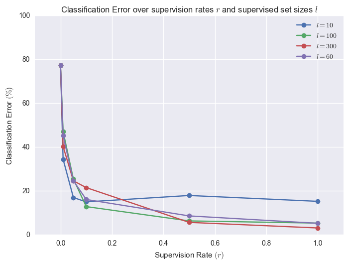
A particular feature of our approach is the ability to learn disentangled representations with just a few labelled data points. Combined with the ability to re-observe a particular labelled data point through the use of the supervision rate, our framework can effectively disentangle the latent representations in a semi-supervised learning regime involving only a handful of labelled data. Figure 2(b) shows how the error rate varies with change in the supervision rate for different labelled set (per class) sizes. Note the steep drop in error rate with just a handful of labels (e.g. 10) seen just a few times (e.g. 1% of the time). The supervision rate here corresponds to sampling minibatches of 80 data points from a total labelled set of 100 data points, with each label class equally represented in the labelled set.

MNIST $l$ Ours “M2” [7] 10 12.2 ($\pm$ 1.38) 11.97 ($\pm$ 1.71) 60 5.28 ($\pm$ 0.76) 4.94 ($\pm$ 0.13) 100 4.23 ($\pm$ 0.68) 3.60 ($\pm$ 0.56) 300 3.94 ($\pm$ 0.77) 3.92 ($\pm$ 0.63) SVHN $l$ Ours “M1+M2” [7] 100 30.32 ($\pm$ 2.74) 36.02 ($\pm$ 0.10) 300 23.98 ($\pm$ 1.83) -
(a)	(b)

Figure 2: (a) Classification-error rates for different (per-class) labelled-set sizes ($l$) over different runs. (b) Classification-error for the MNIST dataset over different labelled set (per class) sizes ($l$) and supervision rates ($r$) = {0, 0.01, 0.05, 0.1, 0.5, 1.0}.

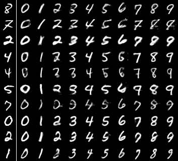
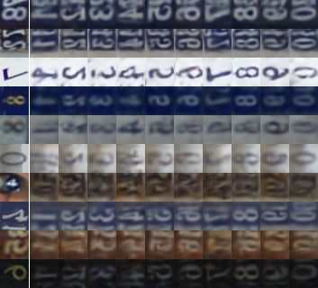
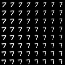
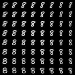
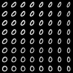
Another means of measuring how well the latent space has been disentangled is by manipulation of the generative model. Here, one can vary the values of particular variables, and observe if the generative model produces outputs that suitably reflect the changes effected. For the datasets and models considered here, this is cast as the visual analogies task. Figure 3 demonstrates the effect of manipulating the latent variables in the learnt generative model in different ways.

Figure 3(a) tests the changes observed in the generative model outputs when the style variable $n$ is held constant, and the digit label $l$ is varied. For both the MNIST and SVHN datasets, it clearly demonstrates that changing only the digit label has the expected effect of varying the class, but maintaining style. Had the latent space not been sufficiently disentangled, this could not be the case.

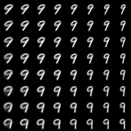
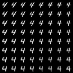
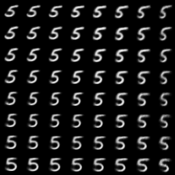
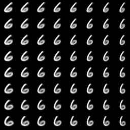
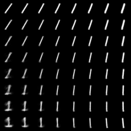
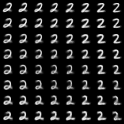
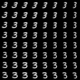
Figure 3(b) tests the changes observed in the generative model outputs in the opposite case, when the digit label $l$ is held constant, and the style variable $l$ is varied, for each of the digits in the MNIST dataset. Note that we only evaluate this capability on the MNIST dataset as this particular exercise needs the style variable to be 2-dimensional, which is just sufficient to capture the variations in MNIST, but is not sufficient to capture variation in the more complex SVHN dataset. Again, we note that digits maintain their identity in the outputs while systematically reflecting changes in style. This also is something that would not be possible had the latents not been sufficiently disentangled.

(a)		(b)

Figure 3: Exploring the disentangled latent space through the generative model. (a) Visual analogies, where the style latent variable $n$ is kept fixed and the label $l$ varied. (b) Exploration in the style $n$ space for a 2D latent Gaussian random variable, keeping label $l$ fixed.

In summary, we demonstrate the utility and efficacy of employing graphical models in the encoders or recognition networks of variational autoencoders to induce interpretable latent representations with semi-supervised learning. Results of experiments conducted with our framework demonstrate, both qualitatively and quantitatively, the practical effectiveness of our framework in learning interpretable and disentangled latent representations.

References

- Bengio et al. [2013] Yoshua Bengio, Nicholas Léonard, and Aaron Courville. Estimating or propagating gradients through stochastic neurons for conditional computation. arXiv preprint arXiv:1308.3432, 2013.
- Collobert et al. [2011] Ronan Collobert, Koray Kavukcuoglu, and Clément Farabet. Torch7: A matlab-like environment for machine learning. In BigLearn, NIPS Workshop, 2011.
- Eslami et al. [2016] S. M. Ali Eslami, Nicolas Heess, Theophane Weber, Yuval Tassa, Koray Kavukcuoglu, and Geoffrey. E Hinton. Attend, infer, repeat: Fast scene understanding with generative models. arXiv preprint arXiv:1603.08575, 2016.
- Johnson et al. [2016] Matthew J. Johnson, David K. Duvenaud, Alex B. Wiltschko, Sandeep R. Datta, and Ryan P. Adams. Composing graphical models with neural networks for structured representations and fast inference. In Advances in Neural Information Processing Systems, 2016.
- Kingma and Ba [2014] Diederik P. Kingma and Jimmy Ba. Adam: A method for stochastic optimization. CoRR, abs/1412.6980, 2014. URL http://arxiv.org/abs/1412.6980.
- Kingma and Welling [2014] Diederik P Kingma and Max Welling. Auto-encoding variational bayes. In Proceedings of the 2nd International Conference on Learning Representations, 2014.
- Kingma et al. [2014] Diederik P Kingma, Shakir Mohamed, Danilo Jimenez Rezende, and Max Welling. Semi-supervised learning with deep generative models. In Advances in Neural Information Processing Systems, pages 3581–3589, 2014.
- Koller and Friedman [2009] Daphne Koller and Nir Friedman. Probabilistic graphical models: principles and techniques. MIT press, 2009.
- Krizhevsky et al. [2012] Alex Krizhevsky, Ilya Sutskever, and Geoffrey E Hinton. Imagenet classification with deep convolutional neural networks. In F. Pereira, C. J. C. Burges, L. Bottou, and K. Q. Weinberger, editors, Advances in Neural Information Processing Systems 25, pages 1097–1105. Curran Associates, Inc., 2012.
- Kulkarni et al. [2015] Tejas D Kulkarni, William F Whitney, Pushmeet Kohli, and Josh Tenenbaum. Deep convolutional inverse graphics network. In Advances in Neural Information Processing Systems, pages 2530–2538, 2015.
- Murphy [2012] Kevin P Murphy. Machine learning: a probabilistic perspective. MIT press, 2012.
- Rezende et al. [2014] Danilo Jimenez Rezende, Shakir Mohamed, and Daan Wierstra. Stochastic backpropagation and approximate inference in deep generative models. In Proceedings of The 31st International Conference on Machine Learning, pages 1278–1286, 2014.
- Schulman et al. [2015] John Schulman, Nicolas Heess, Theophane Weber, and Pieter Abbeel. Gradient estimation using stochastic computation graphs. In Advances in Neural Information Processing Systems, pages 3510–3522, 2015.
- Sohn et al. [2015] Kihyuk Sohn, Honglak Lee, and Xinchen Yan. Learning structured output representation using deep conditional generative models. In Advances in Neural Information Processing Systems, pages 3465–3473, 2015.