The Prior Influence Function in Variational Bayes

Abstract

In Bayesian analysis, the posterior follows from the data and a choice of a prior and a likelihood. One hopes that the posterior is robust to reasonable variation in the choice of prior, since this choice is made by the modeler and is often somewhat subjective. A different, equally subjectively plausible choice of prior may result in a substantially different posterior, and so different conclusions drawn from the data. Were this to be the case, our conclusions would not be robust to the choice of prior. To determine whether our model is robust, we must quantify how sensitive our posterior is to perturbations of our prior.

Variational Bayes (VB) methods are fast, approximate methods for posterior inference. As with any Bayesian method, it is useful to evaluate the robustness of a VB approximate posterior to changes in the prior. In this paper, we derive VB versions of classical non-parametric local robustness measures. In particular, we show that the influence function of Gustafson (2000) has a simple, easy-to-calculate closed form expression for VB approximations. We then demonstrate how local robustness measures can be inadequate for non-local prior changes, such as replacing one prior entirely with another. We propose a simple approximate non-local robustness measure and demonstrate its effectiveness on a simulated data set.

1 Local robustness and the influence function

Bayesian robustness studies how changes to the model (i.e., the prior and likelihood) and to the data affect the posterior. If important aspects of the posterior are meaningfully sensitive to subjectively reasonable perturbations of the inputs, then the posterior is “non-robust” to these perturbations. In this paper, we focus on quantifying the sensitivity of posterior means to perturbations of the prior – either infinitesimally mixing or completely replacing the original prior with another “contaminating prior”. Our methods allow fast estimation of sensitivity to any contaminating prior without re-fitting the model. We follow and extend the work of Gustafson (1996) and Gustafson (2000) to variational Bayes and to approximate non-local measures of sensitivity. For a more general review of Bayesian robustness, see Berger et al. (2000).

We will now define some terminology. Denote our $N$ data points by $x=\left(x_{1},\ldots,x_{N}\right)$ with $x_{n}\in\mathbb{R}^{D}$. Denote our parameter by the vector $\theta\in\mathbb{R}^{K}$. We will suppose that we are interested in the robustness of our prior to a scalar parameter $\epsilon$ where our prior can be written as $p\left(\theta|\epsilon\right)$. Let $p_{\epsilon}^{x}$ denote the posterior distribution of $\theta$ with prior given by $\epsilon$ and conditional on $x$, as given by Bayes’ Theorem: $p_{\epsilon}^{x}\left(\theta\right):=p\left(\theta|x,\epsilon\right)=\frac{p\left(x|\theta\right)p\left(\theta|\epsilon\right)}{p\left(x\right)}$.

A typical end product of a Bayesian analysis might be a posterior expectation of some function, $\mathbb{E}_{p_{\epsilon}^{x}}\left[g\left(\theta\right)\right]$, which is a functional of $g\left(\theta\right)$ and $p_{\epsilon}^{x}\left(\theta\right)$. Local robustness considers how much $\mathbb{E}_{p_{\epsilon}^{x}}\left[g\left(\theta\right)\right]$ changes locally in response to small perturbations in the value of $\epsilon$ (Gustafson, 2000). In the present work, we consider mixing our original prior, $p_{0}\left(\theta\right)$, with some known alternative functional form, $p_{c}\left(\theta\right)$:

$$p\left(\theta|\epsilon\right) = \left(1-\epsilon\right)p_{0}\left(\theta\right)+\epsilon p_{c}\left(\theta\right)\textrm{ for }\epsilon\in\left[0,1\right].$$ (1)

This is known as epsilon contamination (the subscript $c$ stands for “contamination”), and its construction guarantees that the perturbed prior is properly normalized. The contaminating prior, $p_{c}\left(\theta\right)$ need not be in the same parametric family as $p_{0}\left(\theta\right)$, so as $p_{c}\left(\theta\right)$ ranges over all possible priors, (LABEL:epsilon_contamination) represents an expressive class of perturbations. Under mild assumptions (given in A), the local sensitivity measure at the prior $p\left(\theta|\epsilon\right)$ given by a particular $\epsilon$ is

$$S_{\epsilon}^{p_{c}} = \left.\frac{d\mathbb{E}_{p_{\epsilon}^{x}}\left[g\left(\theta\right)\right]}{d\epsilon}\right|_{\epsilon}=\textrm{Cov}_{p_{\epsilon}^{x}}\left(g\left(\theta\right),\frac{p_{c}\left(\theta\right)-p_{0}\left(\theta\right)}{p_{0}\left(\theta\right)+\epsilon\left(p_{c}\left(\theta\right)-p_{0}\left(\theta\right)\right)}\right).$$ (2)

The definition in (LABEL:local_robustness) depends on a choice of $p_{c}\left(\theta\right)$, which we denote with a superscript on $S_{\epsilon}^{p_{c}}$. At $\epsilon=0$, we recover the local sensitivity around $p_{0}\left(\theta\right)$, which we denote $S_{0}^{p_{c}}$.

Rather than choose some finite set of $p_{c}\left(\theta\right)$ and calculate their corresponding $S_{\epsilon}^{p_{c}}$, one can work with a single function that summarizes the effect of any $p_{c}\left(\theta\right)$, called the “influence function” (Gustafson, 2000). Observing that (LABEL:local_robustness) is a linear functional of $p_{c}\left(\theta\right)$ when $g\left(\theta\right)$, $\epsilon$, and $p\left(\theta|\epsilon\right)$ are fixed, the influence function (when it exists) is defined as the linear operator $I_{\epsilon}\left(\theta\right)$ that characterizes the dependence of $S_{\epsilon}^{p_{c}}$ on $p_{c}\left(\theta\right)$:

$$S_{\epsilon}^{p_{c}} = \int I_{\epsilon}\left(\theta\right)p_{c}\left(\theta\right)d\theta\quad\textrm{where}\quad I_{\epsilon}\left(\theta\right):=\frac{p_{\epsilon}^{x}\left(\theta\right)}{p\left(\theta|\epsilon\right)}\left(g\left(\theta\right)-\mathbb{E}_{p_{\epsilon}^{x}}\left[g\left(\theta\right)\right]\right).$$ (3)

At $\epsilon=0$, we recover the local sensitivity around $p_{0}\left(\theta\right)$, which we denote $I_{0}\left(\theta\right)$. When perturbing a low-dimensional marginal of the prior, $I_{0}\left(\theta\right)$ is an easy-to-visualize summary of the effect of sensitivity to an arbitrary $p_{c}\left(\theta\right)$ using quantities calculated only under $p_{0}\left(\theta\right)$ (see the example in 4 and the extended discussion in Gustafson (2000)). Additionally, the worst case prior in a suitably defined metric ball around $p_{0}\left(\theta\right)$ is a functional of the influence function, as shown in Gustafson (2000).

2 Variational approximation and linear response

We now derive a version of (LABEL:local_robustness) for Variational Bayes (VB) approximations to the posterior. Recall that an variational approximate posterior is a distribution selected to minimize the Kullback-Liebler (KL) divergence to $p_{\epsilon}^{x}$ across distributions $q$ in some class $\mathcal{Q}$. Let $q_{\epsilon}^{x}$ denote the variational approximation to posterior $p_{\epsilon}^{x}$. We assume that distributions in $\mathcal{Q}$ are smoothly parameterized by a finite-dimensional parameter $\eta$ whose optimum lies in the interior of some feasible set $\Omega_{\eta}$.

We would like to calculate the local robustness measures of 1 for the variational approximation $q_{\epsilon}^{x}$, but a direct evaluation of the covariance in (LABEL:local_robustness) can be misleading. For example, a common choice of the approximating family$\mathcal{Q}$ is the class of distributions that factorize across $\theta$. This is known as the “mean field approximation” (Wainwright and Jordan, 2008). By construction, a mean field approximation does not model covariances between independent components of $\theta$, so a naive estimate of the covariance in (LABEL:local_robustness) may erroneously suggest that the prior on one component of $\theta$ cannot affect the posterior on another.

However, for VB approximations, we can evaluate the derivative on the left hand side of (LABEL:local_robustness) directly. Using linear response variational Bayes (LRVB) (Giordano et al., 2016, 2015), we have

$$\left.\frac{d}{d\epsilon}\mathbb{E}_{q_{\epsilon}^{x}}\left[g\left(\theta\right)\right]\right|_{\epsilon} = \int\frac{q_{\epsilon}^{x}\left(\theta\right)}{p\left(\theta|\epsilon\right)}q_{\eta}\left(\theta\right)^{T}H^{-1}g_{\eta}p_{c}\left(\theta\right)d\theta$$ (4)

$$\textrm{where }g_{\eta}:=\frac{\partial\mathbb{E}_{q_{\epsilon}^{x}}\left[g\left(\theta\right)\right]}{\partial\eta}\textrm{, }\quad q_{\eta}\left(\theta\right) := \frac{\partial\log q_{\epsilon}^{x}\left(\theta;\eta\right)}{\partial\eta}\textrm{, and }\quad H:=\frac{\partial^{2}KL\left(q_{\epsilon}^{x}\left(\theta;\eta\right)||p_{\epsilon}^{x}\right)}{\partial\eta\partial\eta^{T}}.$$

It follows immediately from the definition in (LABEL:influence_definition) that we can define the variational influence function

$$I_{\epsilon}^{q}\left(\theta\right) :=\frac{q_{\epsilon}^{x}\left(\theta\right)}{p\left(\theta|\epsilon\right)}q_{\eta}\left(\theta\right)^{T}H^{-1}g_{\eta}$$ (5)

that captures the sensitivity of $\mathbb{E}_{q_{\epsilon}^{x}}\left[g\left(\theta\right)\right]$ just as $I_{\epsilon}\left(\theta\right)$ captures the sensitivity of $\mathbb{E}_{p_{\epsilon}^{x}}\left[g\left(\theta\right)\right]$.

The VB versions of epsilon sensitivity measures have some advantages and disadvantages relative to using Markov Chain Monte Carlo (MCMC) to evaluate the exact sensitivities in 1. Using MCMC samples from $p_{0}^{x}$, one can form a Monte Carlo estimate of the covariance in (LABEL:local_robustness), though the sample variance may be infinite when $p_{c}$ has heavier tails than $p_{0}$. The extent to which this is a real problem in practice will vary. Similarly, one must take care in numerically evaluating (LABEL:lrvb_epsilon_sensitivity), since naively sampling from $q_{\epsilon}^{x}$ may also result in infinite variance due to the term $p\left(\theta|\epsilon\right)$ in the denominator. Since we have a closed form for $q_{\epsilon}^{x}$, we can instead evaluate (LABEL:lrvb_epsilon_sensitivity) as an integral over $p_{c}$ using importance sampling, as described in D. Still, providing efficient estimates of (LABEL:lrvb_epsilon_sensitivity) for high-dimensional, non-conjugate, heavy-tailed $p_{c}$ remains a challenge. Finally, in contrast to (LABEL:influence_definition), where we do not generally have a closed form expression for $p_{\epsilon}^{x}$, every term in (LABEL:lrvb_influence_function) is known. This means it is easier to evaluate the influence function for VB approximations than from MCMC draws, especially far from the posterior.

3 Non-local approximation

Equation (3) quantifies the effect of adding an infinitesimal amount of the contaminating prior. In practice, we may also want to evaluate intermediate values of $\epsilon$, particularly $\epsilon=1$, which represents completely replacing $p_{0}\left(\theta\right)$ with $p_{c}\left(\theta\right)$. Since $p_{c}\left(\theta\right)$ may be quite different from $p_{0}\left(\theta\right)$, this is a non-local robustness measure. For MCMC samples, one can use importance sampling, which is essentially equivalent to evaluating the covariance in (LABEL:local_robustness) (with the same problem of infinite variance – see C). For VB, however, we either need to re-fit the model for each new prior (which may be time consuming) or somehow use the local information at $q_{0}^{x}$. In this paper, we investigate the latter. For the remainder of this section, since our results are general, we will discuss using local information in $p_{0}^{x}$. However, the reader should keep in mind that the ultimate goal is to apply the insights gained to the variational approximation $q_{0}^{x}$.

One might hope to linearly extrapolate from $\epsilon=0$ to $\epsilon=1$ using the slope $S_{0}^{p_{c}}$ at $\epsilon=0$. That is, we might hope that $\left.\mathbb{E}_{p_{\epsilon}^{x}}\left[g\left(\theta\right)\right]\right|_{\epsilon=0}^{\epsilon=1}\approx\left(1-0\right)\left.\frac{d\mathbb{E}_{p_{\epsilon}^{x}}\left[g\left(\theta\right)\right]}{d\epsilon}\right|_{\epsilon=0}$. However, as we will now show, this is not realistic when one of the two priors is more consistent with the data than the other. Inspection of (LABEL:influence_definition) shows that posterior expectations are highly sensitive to perturbations of priors which are inconsistent with the data: if $p\left(\theta|\epsilon\right)$ is small in an area of the $\theta$ space where $p_{\epsilon}^{x}$ is not small, then the influence function $I_{\epsilon}\left(\theta\right)$ will be quite large. The model will have high sensitivity to any contaminating prior, $p_{c}\left(\theta\right)$, that is more consistent with the model than $p\left(\theta|\epsilon\right)$ at $\epsilon$. In particular, this is true at $\epsilon=0$ where $p\left(\theta|\epsilon\right)=p_{0}\left(\theta\right)$ if $p_{0}\left(\theta\right)$ is inconsistent with the data. In fact, as we show in A,

$$\left.\mathbb{E}_{p_{\epsilon}^{x}}\left[g\left(\theta\right)\right]\right|_{\epsilon=0}^{\epsilon=1} =\int_{0}^{1}\left.\frac{d\mathbb{E}_{p_{\epsilon}^{x}}\left[g\left(\theta\right)\right]}{d\epsilon}\right|_{\epsilon}d\epsilon=\frac{\int p\left(x|\theta\right)p_{c}\left(\theta\right)d\theta}{\int p\left(x|\theta\right)p_{0}\left(\theta\right)d\theta}S_{0}^{p_{c}}.$$ (6)

When the model evidence is very different for $p_{c}$ and $p_{0}$, e.g. when $\int p\left(x|\theta\right)p_{0}\left(\theta\right)d\theta\ll\int p\left(x|\theta\right)p_{c}\left(\theta\right)d\theta$ as in 4, the extrapolated slope $S_{0}^{p_{c}}$ can be quite different from the effect of replacing completely replacing $p_{0}\left(\theta\right)$ with $p_{c}\left(\theta\right)$.

However, as $\epsilon$ grows away from zero and the new prior $p_{c}\left(\theta\right)$ is taken into account, the influence function will shrink. Observe that as a function of $\epsilon$ (LABEL:local_robustness), one can show (see A) that

$$\left.\frac{d\mathbb{E}_{p_{\epsilon}^{x}}\left[g\left(\theta\right)\right]}{d\epsilon}\right|_{\epsilon} \leq\textrm{max}\left\{\frac{1}{\epsilon},\frac{1}{1-\epsilon}\right\}\mathbb{E}_{p_{\epsilon}^{x}}\left[\left|g\left(\theta\right)-\mathbb{E}_{p_{\epsilon}^{x}}\left[g\left(\theta\right)\right]\right|\right].$$ (7)

For $\epsilon=0$ or $1$, this bound is vacuous, since the ratio $p_{c}\left(\theta\right)/p_{0}\left(\theta\right)$ can be arbitrarily large in areas assigned positive probability by $p_{\epsilon}^{x}$. However, for intermediate values of $\epsilon$, such as $\frac{1}{2}$, the bound is quite strong. In other words, contamination with $p_{c}\left(\theta\right)$ can have great influence on $\mathbb{E}_{p_{\epsilon}^{x}}\left[g\left(\theta\right)\right]$ when $\epsilon$ is close to the boundaries of $\left[0,1\right]$, but once $p_{c}\left(\theta\right)$ is taken into account with intermediate $\epsilon$, its influence is tightly bounded by (LABEL:sensitivity_bound). In this sense, the value of $\left.\frac{d\mathbb{E}_{p_{\epsilon}^{x}}\left[g\left(\theta\right)\right]}{d\epsilon}\right|_{\epsilon}$ is most atypical of its value across the interval $\epsilon\in\left[0,1\right]$ at its endpoints. A real-life example of exactly this phenomenon is shown in 4 in Fig. (1).

This suggests replacing the derivative at $\epsilon=0$ with an average of the derivative over the interval $\epsilon\in\left[0,1\right]$. To do this, note that the difficulty of the integral in (LABEL:global_local_sens_evidence) is the complicated dependence of $p_{\epsilon}^{x}$ on $\epsilon$ in $I_{\epsilon}\left(\theta\right)$. However, we can approximate the integral by keeping $p_{\epsilon}^{x}$ fixed at $p_{0}^{x}$ so that $I_{\epsilon}\left(\theta\right)$ only depends on $\epsilon$ through $p\left(\theta|\epsilon\right)$. Under this approximation, the integral can be evaluated analytically (see B), giving the contaminating pseudo-density, $p_{mv}\left(\theta\right)$, which represents the approximate effect of integrating over $\epsilon$ from $0$ to $1$:

$$\left.\mathbb{E}_{p_{\epsilon}^{x}}\left[g\left(\theta\right)\right]\right|_{\epsilon=0}^{\epsilon=1} \approx\int I_{0}\left(\theta\right)p_{mv}\left(\theta\right)d\theta\quad\quad p_{mv}\left(\theta\right):=\frac{p_{c}\left(\theta\right)p_{0}\left(\theta\right)}{p_{c}\left(\theta\right)-p_{0}\left(\theta\right)}\log\frac{p_{c}\left(\theta\right)}{p_{0}\left(\theta\right)}.$$ (8)

In the notation $p_{mv}\left(\theta\right)$, “mv” stands for “mean value”, by analogy with the mean value theorem for functions of real numbers. As shown in 4, using $p_{mv}\left(\theta\right)$ with $I_{0}\left(\theta\right)$ rather than $p_{c}\left(\theta\right)$ can represent a significant improvement over (LABEL:influence_definition) in practice when extrapolating to $\epsilon=1$. We will focus on using $p_{mv}$ with the variational approximations described in 2.

4 Experiments

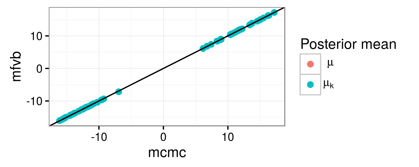
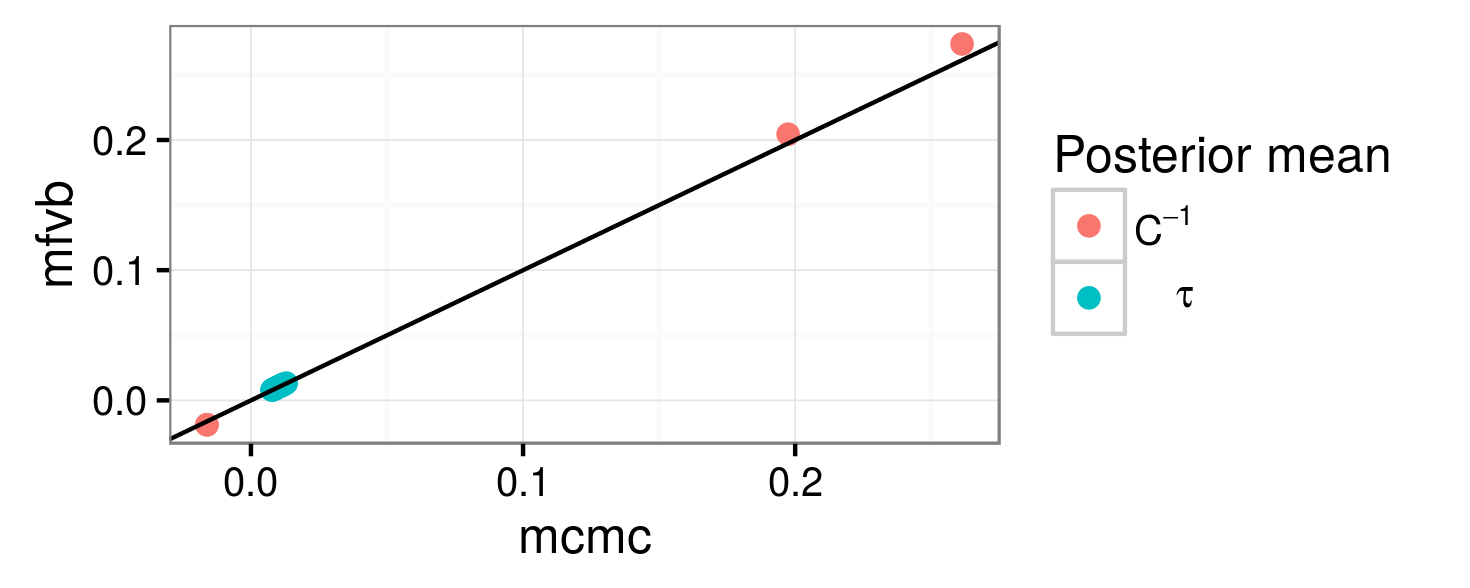
We demonstrate our methods using simulated data from a hierarchical model described in E. Here, we will demonstrate that our sensitivity measures accurately predict the changes in VB solutions. We discuss the close match between the VB and MCMC results in E. The results below are for the sensitivity of the expectation $\mathbb{E}_{p_{0}^{x}}\left[\mu_{11}\right]$ to the prior $p\left(\mu\right)$, though similar results are easily calculated for any other low-dimensional prior marginal or posterior expectation.

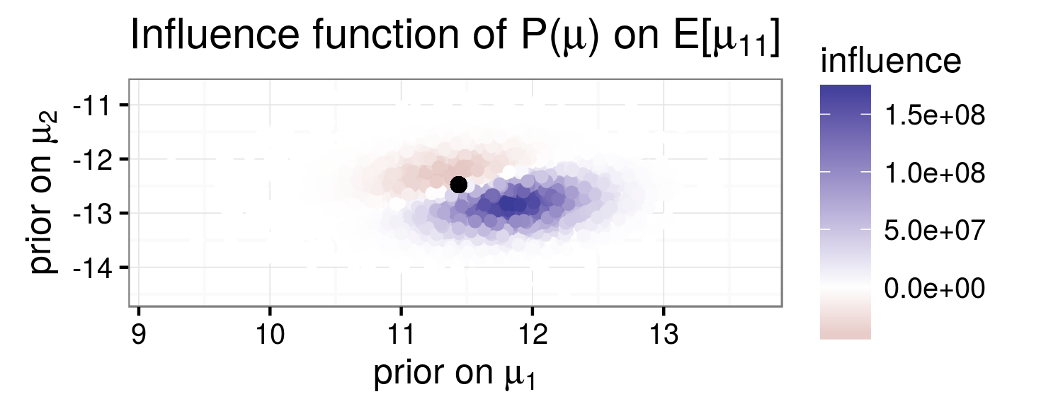
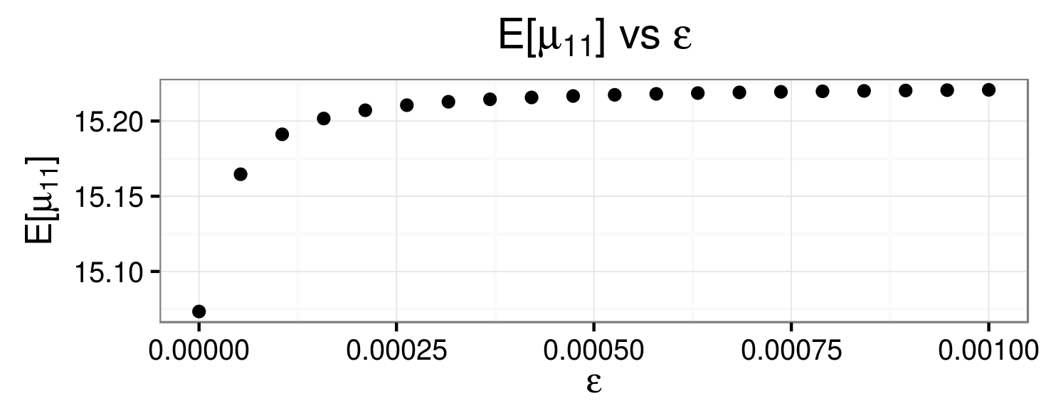
We generate data using true parameters that are far from $p_{0}\left(\theta\right)$ so that our model is not robust to perturbations, as can be seen by the large values of the influence function, which is pictured in the top left panel of Fig. (1). The posterior mean is shown with a black dot, indicating that, though large, the influence function is very highly concentrated around the posterior mean. The top right panel of Fig. (1) indicates how $\mathbb{E}_{q_{\epsilon}^{x}}\left[\mu_{11}\right]$ depends on $\epsilon$ near $\epsilon=0$. The slope is very steep at $\epsilon=0$, reflecting the fact that $p_{c}\left(\theta\right)$ takes values much larger than $p_{0}\left(\theta\right)$ near the posterior where the influence function is very high. However, it very quickly levels off for $\epsilon$ only slightly above zero.

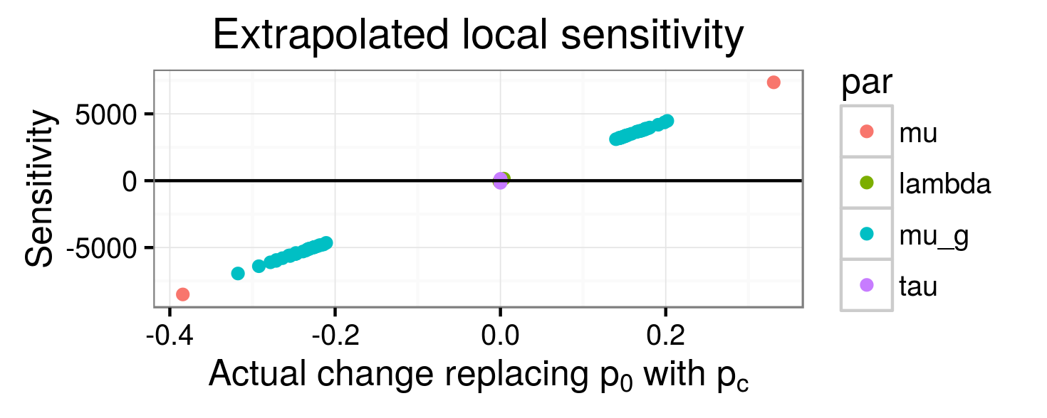
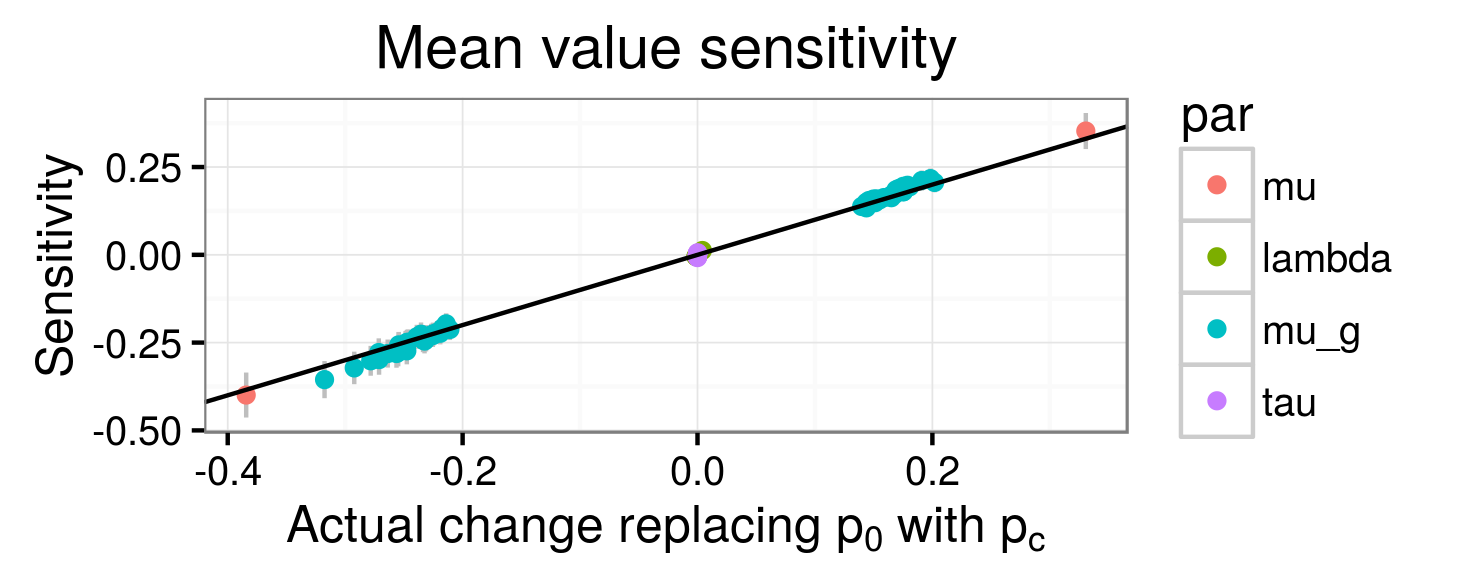
The top right panel of Fig. (1) indicates that extrapolating from the slope $S_{0}^{p_{c}}$ at $\epsilon=0$ will radically over-estimate the effect of replacing $p_{0}\left(\theta\right)$ with $p_{c}\left(\theta\right)$. This is confirmed in the bottom left panel, which has the actual change in $\mathbb{E}_{q_{\epsilon}^{x}}\left[\theta\right]$ on the x-axis and $\int I_{\epsilon}^{q}\left(\theta\right)p_{c}\left(\theta\right)d\theta$ on the y-axis. Clearly, the extrapolation is unrealistic. However, the right panel of Fig. (1) demonstrates that $\int I_{\epsilon}^{q}\left(\theta\right)p_{mv}\left(\theta\right)d\theta$ accurately matches the effect of replacing $p_{0}\left(\theta\right)$ with $p_{c}\left(\theta\right)$. Note the different ranges in the y-axis (which prohibit plotting the two graphs on the same scale). The error bars represent importance sampling error.

Figure 1: Simulation results

Acknowledgements

The paper was greatly improved through the insightful comments of our anonymous reviewers. Ryan Giordano was supported by the Director, Office of Science, Office of Advanced Scientific Computing Research, Applied Mathematics program of the U.S. Department of Energy under Contract No. DE-AC02-05CH1123.

Appendices

Appendix A Epsilon sensitivity

Throughout the paper, we make the following assumptions:

• Assumption 1. For all $\epsilon\in\left[0,1\right]$, $p\left(\theta|\epsilon\right)$ is strictly positive where $\theta$ has positive measure.

• Assumption 2. Both $p\left(\theta|x\right)$ and $g\left(\theta\right)p\left(\theta|x\right)$ are bounded as a function of $\theta$ .

Under these assumptions, (LABEL:local_robustness) follows directly from Gustafson [1996] result 8. For completeness, we reproduce a slightly simpler proof under the slightly less clearly-articulated assumption that we can exchange integration and differentiation as described, for example, in Durrett [2010, Appendix A.5]. Denote by $p\left(\theta|\epsilon\right)$ any distribution parameterized by the scalar $\epsilon$ (not necessarily a prior). Then by direct differentiation,

$$\frac{d\mathbb{E}_{p\left(\theta|\epsilon\right)}\left[g\left(\theta\right)\right]}{d\epsilon} =\frac{d}{d\epsilon}\int p\left(\theta|\epsilon\right)g\left(\theta\right)d\theta$$

$$=\int\frac{dp\left(\theta|\epsilon\right)}{d\epsilon}g\left(\theta\right)d\theta$$

$$=\int\frac{d\log p\left(\theta|\epsilon\right)}{d\epsilon}p\left(\theta|\epsilon\right)g\left(\theta\right)d\theta.$$ (9)

By applying (LABEL:differentiate_under_integral) to $g\left(\theta\right)=1$, we see that $\mathbb{E}_{p\left(\theta|\epsilon\right)}\left[\frac{d\log p\left(\theta|\epsilon\right)}{d\epsilon}\right]=\int\frac{d\log p\left(\theta|\epsilon\right)}{d\epsilon}p\left(\theta|\epsilon\right)d\theta=0$, so we can subtract $0=\mathbb{E}_{p\left(\theta|\epsilon\right)}\left[g\left(\theta\right)\right]\mathbb{E}_{p\left(\theta|\epsilon\right)}\left[\frac{d\log p\left(\theta|\epsilon\right)}{d\epsilon}\right]$ to get

$$\frac{d\mathbb{E}_{p\left(\theta|\epsilon\right)}\left[g\left(\theta\right)\right]}{d\epsilon} =\textrm{Cov}_{p\left(\theta|\epsilon\right)}\left(g\left(\theta\right),\frac{d\log p\left(\theta|\epsilon\right)}{d\epsilon}\right).$$ (10)

To derive (LABEL:local_robustness), we simply observe that

$$\frac{d\log p\left(\theta|\epsilon\right)}{d\epsilon} =\frac{d}{d\epsilon}\log\left(\left(1-\epsilon\right)p_{0}\left(\theta\right)+\epsilon p_{c}\left(\theta\right)\right)$$

$$=\frac{p_{c}\left(\theta\right)-p_{0}\left(\theta\right)}{p_{0}\left(\theta\right)+\epsilon\left(p_{c}\left(\theta\right)-p_{0}\left(\theta\right)\right)}.$$

Note that the assumptions also suffice to assure that the covariance is bounded.

Next, we observe the simple relationship between epsilon sensitivity at $\epsilon=0$ and the effect of replacing one prior with another. First, defining the normalizing constants

$$C_{0} :=\int p\left(x|\theta\right)p_{0}\left(\theta\right)d\theta$$

$$C_{1} :=\int p\left(x|\theta\right)p_{c}\left(\theta\right)d\theta$$

$$\mathbb{E}_{p_{0}^{x}}\left[\frac{p_{c}\left(\theta\right)}{p_{0}\left(\theta\right)}\right] =\int\frac{p\left(x|\theta\right)p_{0}\left(\theta\right)}{C_{0}}\frac{p_{c}\left(\theta\right)}{p_{0}\left(\theta\right)}d\theta=\frac{C_{1}}{C_{0}},$$

by straightforward manipulation we have

$$\left.\mathbb{E}_{p_{\epsilon}^{x}\left(\theta\right)}\left[g\left(\theta\right)\right]\right|_{\epsilon=1}-\left.\mathbb{E}_{p_{\epsilon}^{x}\left(\theta\right)}\left[g\left(\theta\right)\right]\right|_{\epsilon=0} =\int\frac{p\left(x|\theta\right)p_{c}\left(\theta\right)}{C_{1}}g\left(\theta\right)d\theta-\mathbb{E}_{p_{0}^{x}\left(\theta\right)}\left[g\left(\theta\right)\right]$$

$$=\int\frac{p\left(x|\theta\right)p_{c}\left(\theta\right)}{C_{1}}\frac{p_{0}\left(\theta\right)}{C_{0}}\frac{C_{0}}{p_{0}\left(\theta\right)}g\left(\theta\right)d\theta-\frac{C_{0}}{C_{1}}\mathbb{E}_{p_{0}^{x}}\left[\frac{p_{c}\left(\theta\right)}{p_{0}\left(\theta\right)}\right]\mathbb{E}_{p_{0}^{x}\left(\theta\right)}\left[g\left(\theta\right)\right]$$

$$=\frac{C_{0}}{C_{1}}\left(\mathbb{E}_{p_{0}^{x}\left(\theta\right)}\left[\frac{p_{c}\left(\theta\right)}{p_{0}\left(\theta\right)}g\left(\theta\right)\right]-\mathbb{E}_{p_{0}^{x}}\left[\frac{p_{c}\left(\theta\right)}{p_{0}\left(\theta\right)}\right]\mathbb{E}_{p_{0}^{x}\left(\theta\right)}\left[g\left(\theta\right)\right]\right)$$

$$=\frac{C_{0}}{C_{1}}\textrm{Cov}_{p_{0}^{x}\left(\theta\right)}\left(g\left(\theta\right),\frac{p_{c}\left(\theta\right)}{p_{0}\left(\theta\right)}\right)$$

$$=\frac{C_{0}}{C_{1}}\left.\frac{d\mathbb{E}_{p_{\epsilon}^{x}}\left[g\left(\theta\right)\right]}{d\epsilon}\right|_{\epsilon=0}.$$

Finally, we derive (LABEL:sensitivity_bound) using (LABEL:local_robustness):

$$\left|\left.\frac{d\mathbb{E}_{p_{\epsilon}^{x}}\left[g\left(\theta\right)\right]}{d\epsilon}\right|_{\epsilon}\right| =\left|\textrm{Cov}_{p_{\epsilon}^{x}}\left(g\left(\theta\right),\frac{p_{c}\left(\theta\right)-p_{0}\left(\theta\right)}{p_{0}\left(\theta\right)+\epsilon\left(p_{c}\left(\theta\right)-p_{0}\left(\theta\right)\right)}\right)\right|$$

$$\leq\mathbb{E}_{p_{\epsilon}^{x}}\left[\left|g\left(\theta\right)-\mathbb{E}_{p_{\epsilon}^{x}}\left[g\left(\theta\right)\right]\right|\right]B_{\epsilon}$$

where

$$B_{\epsilon} =\sup_{\theta}\left|\frac{p_{c}\left(\theta\right)-p_{0}\left(\theta\right)}{p_{0}\left(\theta\right)+\epsilon\left(p_{c}\left(\theta\right)-p_{0}\left(\theta\right)\right)}\right|$$

$$=\sup_{\theta}\begin{cases}\frac{p_{c}\left(\theta\right)-p_{0}\left(\theta\right)}{p_{0}\left(\theta\right)+\epsilon\left(p_{c}\left(\theta\right)-p_{0}\left(\theta\right)\right)}&\textrm{when }p_{c}\left(\theta\right)>p_{0}\left(\theta\right)\\ \frac{p_{0}\left(\theta\right)-p_{c}\left(\theta\right)}{p_{0}\left(\theta\right)+\epsilon\left(p_{c}\left(\theta\right)-p_{0}\left(\theta\right)\right)}&\textrm{when }p_{c}\left(\theta\right)\leq p_{0}\left(\theta\right)\end{cases}$$

$$=\sup_{\theta}\begin{cases}\frac{p_{c}\left(\theta\right)-p_{0}\left(\theta\right)}{p_{0}\left(\theta\right)+\epsilon\left(p_{c}\left(\theta\right)-p_{0}\left(\theta\right)\right)}&\textrm{when }p_{c}\left(\theta\right)>p_{0}\left(\theta\right)\\ \frac{p_{0}\left(\theta\right)-p_{c}\left(\theta\right)}{p_{c}\left(\theta\right)+\left(1-\epsilon\right)\left(p_{0}\left(\theta\right)-p_{c}\left(\theta\right)\right)}&\textrm{when }p_{c}\left(\theta\right)\leq p_{0}\left(\theta\right)\end{cases}$$

$$\leq\sup_{\theta}\begin{cases}\frac{p_{c}\left(\theta\right)-p_{0}\left(\theta\right)}{\epsilon\left(p_{c}\left(\theta\right)-p_{0}\left(\theta\right)\right)}&\textrm{when }p_{c}\left(\theta\right)>p_{0}\left(\theta\right)\\ \frac{p_{0}\left(\theta\right)-p_{c}\left(\theta\right)}{\left(1-\epsilon\right)\left(p_{0}\left(\theta\right)-p_{c}\left(\theta\right)\right)}&\textrm{when }p_{c}\left(\theta\right)\leq p_{0}\left(\theta\right)\end{cases}$$

$$\leq\textrm{max}\left\{\frac{1}{\epsilon},\frac{1}{1-\epsilon}\right\}.$$

Appendix B Mean Value Contaminating Prior

Under the assumption that $p_{\epsilon}^{x}\approx p_{0}^{x}$,

$$\left.\mathbb{E}_{p_{\epsilon}^{x}}\left[g\left(\theta\right)\right]\right|_{\epsilon=1}-\left.\mathbb{E}_{p_{\epsilon}^{x}}\left[g\left(\theta\right)\right]\right|_{\epsilon=0} =\int_{0}^{1}\int\frac{p_{\epsilon}^{x}\left(\theta\right)p_{c}\left(\theta\right)}{p\left(\theta|\epsilon\right)}\left(g\left(\theta\right)-\mathbb{E}_{\left.p_{\epsilon}^{x}\left(\theta\right)\right|_{\epsilon=0}}\left[g\left(\theta\right)\right]\right)d\theta d\epsilon$$

$$\approx\int_{0}^{1}\int\frac{p_{0}^{x}\left(\theta\right)p_{c}\left(\theta\right)}{p\left(\theta|\epsilon\right)}\left(g\left(\theta\right)-\mathbb{E}_{\left.p_{\epsilon}^{x}\left(\theta\right)\right|_{\epsilon=0}}\left[g\left(\theta\right)\right]\right)d\theta d\epsilon$$

$$=\int p_{0}^{x}\left(\theta\right)\left(g\left(\theta\right)-\mathbb{E}_{p_{0}^{x}\left(\theta\right)}\left[g\left(\theta\right)\right]\right)\int_{0}^{1}\frac{p_{c}\left(\theta\right)}{p\left(\theta|\epsilon\right)}d\epsilon d\theta$$

$$=\int p_{0}^{x}\left(\theta\right)\left(g\left(\theta\right)-\mathbb{E}_{p_{0}^{x}\left(\theta\right)}\left[g\left(\theta\right)\right]\right)\frac{p_{c}\left(\theta\right)}{p_{c}\left(\theta\right)-p_{0}\left(\theta\right)}\left(\log p_{c}\left(\theta\right)-\log p_{0}\left(\theta\right)\right)d\theta$$

$$=\int I_{0}\left(\theta\right)\frac{p_{c}\left(\theta\right)p_{0}\left(\theta\right)}{p_{c}\left(\theta\right)-p_{0}\left(\theta\right)}\left(\log p_{c}\left(\theta\right)-\log p_{0}\left(\theta\right)\right)d\theta.$$

Where we have used

$$\int_{0}^{1}\frac{p_{c}\left(\theta\right)}{p\left(\theta|\epsilon\right)}d\epsilon =\int_{0}^{1}\frac{p_{c}\left(\theta\right)}{\left(1-\epsilon\right)p_{0}\left(\theta\right)+\epsilon p_{c}\left(\theta\right)}d\epsilon$$

$$=\frac{p_{c}\left(\theta\right)}{p_{c}\left(\theta\right)-p_{0}\left(\theta\right)}\int_{0}^{1}\frac{d}{d\epsilon}\log\left(\left(1-\epsilon\right)p_{0}\left(\theta\right)+\epsilon p_{c}\left(\theta\right)\right)d\epsilon$$

$$=\frac{p_{c}\left(\theta\right)}{p_{c}\left(\theta\right)-p_{0}\left(\theta\right)}\left(\log p_{c}\left(\theta\right)-\log p_{0}\left(\theta\right)\right).$$

Consequently, applying (LABEL:influence_definition) with the pseudo-density

$$p_{mv} :=\frac{p_{c}\left(\theta\right)p_{0}\left(\theta\right)}{p_{c}\left(\theta\right)-p_{0}\left(\theta\right)}\left(\log p_{c}\left(\theta\right)-\log p_{0}\left(\theta\right)\right)$$

represents an approximation to the quantity $\left.\mathbb{E}_{p_{\epsilon}^{x}}\left[g\left(\theta\right)\right]\right|_{\epsilon=1}-\left.\mathbb{E}_{p_{\epsilon}^{x}}\left[g\left(\theta\right)\right]\right|_{\epsilon=0}$, which is the effect of completely replacing $p_{0}\left(\theta\right)$ with $p_{c}\left(\theta\right)$.

Appendix C Comparison with MCMC importance sampling

In this section, we show that using importance sampling with MCMC samples to calculate the local sensitivity (LABEL:local_robustness) is precisely equivalent to using the same MCMC samples to estimate the covariance in (LABEL:covariance_sensitivity) directly. Suppose, without loss of generality, we have samples $\theta_{i}$ drawn from $p_{0}^{x}\left(\theta\right)$

$$\theta_{i} \sim p_{0}^{x}\left(\theta\right)$$

$$\mathbb{E}_{p_{0}^{x}}\left[g\left(\theta\right)\right] \approx\sum_{i}g\left(\theta_{i}\right).$$

If we could calculate the normalizing constants, the importance sampling estimate for $\mathbb{E}_{p_{\epsilon}^{x}}\left[g\left(\theta\right)\right]$ would be

$$\mathbb{E}_{p_{\epsilon}^{x}}\left[g\left(\theta\right)\right] \approx\frac{1}{N}\sum_{i}w_{i}g\left(\theta_{i}\right)$$

$$w_{i} :=\frac{p_{\epsilon}^{x}\left(\theta\right)}{p_{0}^{x}\left(\theta\right)}=\frac{p\left(x|\theta\right)p\left(\theta|\epsilon\right)}{C_{\epsilon}}\frac{C_{0}}{p\left(x|\theta\right)p_{0}\left(\theta\right)}$$

$$=\exp\left(\log p\left(\theta|\epsilon\right)-\log p_{0}\left(\theta\right)+\log C_{0}-\log C_{\epsilon}\right)$$

$$C_{0} :=\int p\left(x|\theta\right)p_{0}\left(\theta\right)d\theta$$

$$C_{\epsilon} :=\int p\left(x|\theta\right)p\left(\theta|\epsilon\right)d\theta.$$

Differentiating the weights,

$$\frac{dw_{i}}{d\epsilon} =w_{i}\left(\frac{d\log p\left(\theta|\epsilon\right)}{d\epsilon}-\frac{d\log C_{\epsilon}}{d\epsilon}\right)$$

$$=w_{i}\left(\frac{d\log p\left(\theta|\epsilon\right)}{d\epsilon}-\frac{1}{C_{\epsilon}}\int p\left(x|\theta\right)p\left(\theta|\epsilon\right)\frac{d\log p\left(\theta|\epsilon\right)}{d\epsilon}d\theta\right)$$

$$=w_{i}\left(\frac{d\log p\left(\theta|\epsilon\right)}{d\epsilon}-\mathbb{E}_{p_{\epsilon}^{x}}\left[\frac{d\log p\left(\theta|\epsilon\right)}{d\epsilon}\right]\right).$$

It follows that

$$\left.\frac{d}{d\epsilon}\frac{1}{N}\sum_{i}w_{i}g\left(\theta_{i}\right)\right|_{\epsilon} =\frac{1}{N}\sum_{i}w_{i}\left(\frac{d\log p\left(\theta_{i}|\epsilon\right)}{d\epsilon}-\mathbb{E}_{p_{\epsilon}^{x}}\left[\frac{d\log p\left(\theta|\epsilon\right)}{d\epsilon}\right]\right)g\left(\theta_{i}\right)$$

which is precisely the MCMC estimate of the covariance given by (LABEL:local_robustness). In particular, when $\epsilon=0$, we have

$$\left.\frac{d}{d\epsilon}\frac{1}{N}\sum_{i}w_{i}g\left(\theta_{i}\right)\right|_{\epsilon=0} =\frac{1}{N}\sum_{i}\left(\frac{p_{c}\left(\theta_{i}\right)}{p_{0}\left(\theta_{i}\right)}-\mathbb{E}_{p_{\epsilon}^{x}}\left[\frac{p_{c}\left(\theta\right)}{p_{0}\left(\theta\right)}\right]\right)g\left(\theta_{i}\right)$$

and the importance sampling estimate for replacing $p_{0}$ with $p_{c}$ is

$$\left.\sum_{i}w_{i}g\left(\theta_{i}\right)\right|_{\epsilon=1} =\frac{1}{N}\sum_{i}\left(\frac{C_{0}p_{c}\left(\theta_{i}\right)}{C_{1}p_{0}\left(\theta_{i}\right)}-\mathbb{E}_{p_{\epsilon}^{x}}\left[\frac{p_{c}\left(\theta_{i}\right)}{p_{0}\left(\theta_{i}\right)}\right]\right)g\left(\theta_{i}\right)$$

$$=\frac{C_{0}}{C_{1}}\left.\frac{d}{d\epsilon}\frac{1}{N}\sum_{i}w_{i}g\left(\theta_{i}\right)\right|_{\epsilon=0}$$

which confirms that the importance sampling estimate is exactly the Monte Carlo analogue of the relation (LABEL:global_local_sens_evidence).

In general, we do not know $C_{0}$ and $C_{\epsilon}$ and must use instead

$$\omega_{i} :=\frac{p\left(\theta|\epsilon\right)}{p_{0}\left(\theta\right)}$$

$$\tilde{\omega}_{i} :=\frac{\omega_{i}}{\sum_{j}\omega_{j}}.$$

Then

$$\frac{d\tilde{\omega}_{i}}{d\epsilon} =\frac{\omega_{i}}{\sum_{j}\omega_{j}}\frac{d\log p\left(\theta_{i}|\epsilon\right)}{d\epsilon}-\frac{\omega_{i}}{\left(\sum_{k}\omega_{k}\right)^{2}}\sum_{j}\omega_{j}\frac{d\log p\left(\theta_{j}|\epsilon\right)}{d\epsilon}$$

$$=\frac{\omega_{i}}{\sum_{j}\omega_{j}}\left(\frac{d\log p\left(\theta_{i}|\epsilon\right)}{d\epsilon}-\sum_{j}\frac{\omega_{j}}{\sum_{k}\omega_{k}}\frac{d\log p\left(\theta_{j}|\epsilon\right)}{d\epsilon}\right)$$

which simply replaces the (possibly intractable) expectation $\mathbb{E}_{p_{\epsilon}^{x}}\left[\frac{d\log p\left(\theta|\epsilon\right)}{d\epsilon}\right]$ with its MCMC estimate.

Appendix D Variational Bayes importance sampling

To evaluate (LABEL:lrvb_epsilon_sensitivity) requires approximate integration for which we using importance sampling:

$$\theta_{s} \sim u\left(\theta\right),\textrm{ for }s=1:S$$

$$w_{s} :=\frac{p_{c}\left(\theta_{s}\right)}{u\left(\theta_{s}\right)}$$

$$\int\frac{q_{0}^{x}\left(\theta\right)}{p_{0}\left(\theta\right)}q_{\eta}\left(\theta\right)^{T}H^{-1}g_{\eta}p_{c}\left(\theta\right)d\theta \approx\frac{1}{S}\sum_{s=1}^{S}\frac{q_{0}^{x}\left(\theta_{s}\right)}{p_{0}\left(\theta_{s}\right)}q_{\eta}\left(\theta_{s}\right)^{T}H^{-1}g_{\eta}w_{s}$$

$$=\frac{1}{S}\sum_{s=1}^{S}I_{0}^{q}\left(\theta_{s}\right)w_{s}.$$

Note that the influence function can be evaluated once for a large number of draws from $u\left(\theta\right)$, and then the weights and prior density can be quickly calculated for any perturbation $p_{c}\left(\theta\right)$, allowing for fast computation of sensitivity to any $p_{c}\left(\theta\right)$ with little additional overhead.

Since the influence function is mostly concentrated around $q_{0}^{x}\left(\theta\right)$, we set $u\left(\theta\right)$ to be $q_{0}^{x}\left(\theta\right)$ but with quadrupled variance (so that standard deviations are doubled). Note that this choice of $u$ is a poor approximation of $p_{c}$, which is nominally the target distribution for importance sampling. However, since $I_{0}^{q}\left(\theta\right)$ is very small far from $q_{0}^{x}\left(\theta\right)$, it is an adequate approximation of the integral (LABEL:lrvb_epsilon_sensitivity). Formally, suppose that $I_{0}^{q}\left(\theta\right)$ is concentrated on a set $A$ in the sense that $\sup_{\theta\in A^{c}}\left|I_{0}^{q}\left(\theta\right)\right|\leq\epsilon$ for some small $\delta$. Then the absolute error in evaluating (LABEL:lrvb_epsilon_sensitivity) on the set $A$ only is also bounded by $\delta$:

$$\left|\int I_{0}^{q}\left(\theta\right)p_{c}\left(\theta\right)d\theta-\int_{A}I_{0}^{q}\left(\theta\right)p_{c}\left(\theta\right)d\theta\right| =\left|\int_{A^{c}}I_{0}^{q}\left(\theta\right)p_{c}\left(\theta\right)d\theta\right|$$

$$\leq\int_{A^{c}}\left|I_{0}^{q}\left(\theta\right)\right|p_{c}\left(\theta\right)d\theta$$

$$\leq\sup_{\theta\in A^{c}}\left|I_{0}^{q}\left(\theta\right)\right|\int_{A^{c}}p_{c}\left(\theta\right)d\theta$$

$$\leq\delta.$$

As long as $q_{\epsilon}^{x}\left(\theta\right)$ is chosen to have lighter tails than $p_{0}\left(\theta\right)$ (which is determined by $\mathcal{Q}$), $I_{0}^{q}\left(\theta\right)$ will decay quickly away from $q_{0}^{x}\left(\theta\right)$, and we can choose $A$ centered on $q_{0}^{x}\left(\theta\right)$. Consequently, we can think of $u$ as approximating $p_{c}\left(\theta\right)1_{A}$ rather than $p_{c}\left(\theta\right)$.

Appendix E Microcredit model

We simulate data using a variant of the analysis performed in [Meager, 2015], though with somewhat different prior choices. In Meager [2015], randomized controlled trials were run in seven different sites to try to measure the effect of access to microcredit on various measures of business success. Each trial was found to lack power individually for various reasons, so there could be some benefit to pooling the results in a simple hierarchical model. For the purposes of demonstrating robust Bayes techniques with VB, we will focus on the simpler of the two models in [Meager, 2015] and ignore covariate information.

We will index sites with $k=1,..,K$ (here, $K=30$) and business within a site by $i=1,...,N_{k}$. The total number of observations was $\sum_{k}N_{k}=3000$. In site $k$ and business $i$ we observe whether the business was randomly selected for increased access to microcredit, denoted $T_{ik}$, and the profit after intervention, $y_{ik}$. We follow [Rubin, 1981] and assume that each site has an idiosyncratic average profit, $\mu_{k1}$ and average improvement in profit, $\mu_{k2}$, due to the intervention. Given $\mu_{k}$, $\tau_{k}$, and $T_{ik}$, the _observed profit is assumed to be generated according to

$$y_{ik}|\mu_{k},\tau_{k},x_{ik},\sigma_{k} \sim N\left(\mu_{k}^{T}x_{ik},\sigma_{k}^{2}\right)$$

$$x_{ik} := \left(\begin{array}[]{c}1\\ T_{ik}\end{array}\right).$$

The site effects, $\mu_{k}$, are assumed to come from an overall pool of effects and may be correlated:

$$\mu_{k}|\mu \sim N\left(\mu,C\right)$$

$$C := \left(\begin{array}[]{cc}\sigma_{\mu}^{2}&\sigma_{\mu\tau}\\ \sigma_{\mu\tau}&\sigma_{\tau}^{2}\end{array}\right).$$

The effects $\mu$ and the covariance matrix $V$ are unknown parameters that require priors. For $\mu$ we simply use a bivariate normal prior. However, choosing an appropriate prior for a covariance matrix can be conceptually difficult [Barnard et al., 2000]. Following the recommended practice of the software package STAN [Stan Team, 2015], we derive a variational model to accommodate the non-conjugate LKJ prior [Lewandowski et al., 2009], allowing the user to model the covariance and marginal variances separately. Specifically, we use

$$C =: SRS$$

$$S =$$ Diagonal matrix

$$R =$$ Covariance matrix

$$S_{kk} = \sqrt{\textrm{diag}(C)_{k}}$$

We can then put independent priors on the scale of the variances, $S_{kk}$, and on the covariance matrix, $R$. We model the inverse of $C$ with a Wishart variational distribution, and use the following priors:

$$q\left(C^{-1}\right) = \textrm{Wishart}\left(V_{\Lambda},n\right)$$

$$p_{0}\left(S\right) = \prod_{k=1}^{2}p\left(S_{kk}\right)$$

$$S_{kk}^{2} \sim \textrm{InverseGamma}\left(\alpha_{scale},\beta_{scale}\right)$$

$$\log p_{0}\left(R\right) = \left(\eta-1\right)\log|R|+C$$

The necessary expectations have closed forms with the Wishart variational approximation, as derived in Giordano et al. [2016]. In addition, we put a normal prior on $(\mu,\tau)^{T}$ and an inverse gamma prior on $\sigma_{k}^{2}$:

$$p_{0}\left(\mu\right) = N\left(0,\Lambda^{-1}\right)$$ (13)

$$p_{0}\left(\sigma_{k}^{2}\right) = \textrm{InverseGamma}\left(\alpha_{\tau},\beta_{\tau}\right)$$

The prior parameters used were:

$$\Lambda = \left(\begin{array}[]{cc}0.111&0\\ 0&0.111\end{array}\right)$$

$$\eta = 15.010$$

$$\sigma_{k}^{-2} \sim \textrm{InverseGamma}(2.010,2.010)$$

$$\alpha_{scale} = 20.010$$

$$\beta_{scale} = 20.010$$

$$\alpha_{\tau} = 2.010$$

$$\beta_{\tau} = 2.010$$

As seen in Fig. (2) , the means in VB and MCMC match closely.

Figure 2: Comparison with MCMC

In our simulation, $\mu$ and $\mu_{k}$ are in $\mathbb{R}^{2}$, so the domain of the prior $p_{0}$$\left(\mu\right)$ is two-dimensional and $I_{0}^{q}\left(\theta\right)$ can be easily visualized. We consider the problem of estimating the effect of replacing the prior on $\mu$ with a product of independent centered Student t priors. In the notation of 1, we take

$$p_{0}\left(\mu\right) =\mathcal{N}\left(\mu_{1};0,\Lambda^{-1}\right)\cdot\mathcal{N}\left(\mu_{2};0,\Lambda^{-1}\right)\quad\quad p_{c}\left(\theta\right)=\textrm{Student}\left(\mu_{1};\nu\right)\cdot\textrm{Student}\left(\mu_{2};\nu\right).$$

We leave all other priors the same, i.e. $p_{0}\left(\tau_{k}\right)=p_{c}\left(\tau_{k}\right)$ and $p_{0}\left(C\right)=p_{c}\left(C\right)$. In our case, we used $\nu=1$ and $\Lambda=0.111$. We will present sensitivity of $\mathbb{E}_{q_{\epsilon}^{x}}\left[\mu_{11}\right]$, the first component of the first top-level effect. In the notation of 1, we are taking $g\left(\theta\right)=\mu_{11}$. Most of the computation is in generating draws and values for the importance sampling of the influence function, which can be done once and then reused for any choice of $p_{c}\left(\theta\right)$ and $g\left(\theta\right)$.

References

- Barnard et al. [2000] John Barnard, Robert McCulloch, and Xiao-Li Meng. Modeling covariance matrices in terms of standard deviations and correlations, with application to shrinkage. Statistica Sinica, 10(4):1281–1312, 2000.
- Berger et al. [2000] James O. Berger, David Ríos Insua, and Fabrizio Ruggeri. Robust Bayesian analysis. In David Ríos Insua and Fabrizio Ruggeri, editors, Robust Bayesian Analysis, volume 152. Springer Science & Business Media, 2000.
- Durrett [2010] Rick Durrett. Probability: theory and examples. Cambridge University Press, 2010.
- Giordano et al. [2015] Ryan Giordano, Tamara Broderick, and Michael Jordan. Linear response methods for accurate covariance estimates from mean field variational Bayes. arXiv preprint arXiv:1506.04088, 2015.
- Giordano et al. [2016] Ryan Giordano, Tamara Broderick, Rachael Meager, Jonathan Huggins, and Michael Jordan. Fast robustness quantification with variational Bayes. arXiv preprint arXiv:1606.07153, 2016.
- Gustafson [1996] Paul Gustafson. Local sensitivity of posterior expectations. The Annals of Statistics, 24(1):174–195, 1996.
- Gustafson [2000] Paul Gustafson. Local robustness in Bayesian analysis. In David Ríos Insua and Fabrizio Ruggeri, editors, Robust Bayesian Analysis, volume 152. Springer Science & Business Media, 2000.
- Lewandowski et al. [2009] Daniel Lewandowski, Dorota Kurowicka, and Harry Joe. Generating random correlation matrices based on vines and extended onion method. Journal of multivariate analysis, 100(9):1989–2001, 2009.
- Meager [2015] Rachael Meager. Understanding the impact of microcredit expansions: A Bayesian hierarchical analysis of 7 randomised experiments. arXiv preprint arXiv:1506.06669, 2015.
- Rubin [1981] Donald B Rubin. Estimation in parallel randomized experiments. Journal of Educational and Behavioral Statistics, 6(4):377–401, 1981.
- Stan Team [2015] Stan Team. Stan Modeling Language Users Guide and Reference Manual, Version 2.8.0, 2015. URL http://mc-stan.org/.
- Wainwright and Jordan [2008] M. J. Wainwright and M. I. Jordan. Graphical models, exponential families, and variational inference. Foundations and Trends® in Machine Learning, 1(1-2):1–305, 2008.