11institutetext: X. G. Zhu 22institutetext: Y. F. Nie 33institutetext: W. W. Zhang44institutetext: Department of Applied Mathematics, Northwestern Polytechnical University, Xi’an, Shaanxi 710129, P. R. China
44email: yfnie@nwpu.edu.cn
55institutetext: X. G. Zhu 66institutetext: 66email: zhuxg590@yeah.net 77institutetext: W. W. Zhang 88institutetext: 88email: wwzhang@nwpu.edu.cn

An efficient differential quadrature method for fractional advection-diffusion equation

X. G. Zhu    Y. F. Nie    W. W. Zhang
(Received: date / Accepted: date)
Abstract

This article studies a direct numerical approach for fractional advection-diffusion equations (ADEs). Using a set of cubic trigonometric B-splines as test functions, a differential quadrature (DQ) method is firstly proposed for the 1D and 2D time-fractional ADEs of order (0,1]01(0,1]. The weighted coefficients are determined, and with them, the original equation is transformed into a group of general ordinary differential equations (ODEs), which are discretized by an effective difference scheme or Runge-Kutta method. The stability is investigated under a mild theoretical condition. Secondly, based on a set of cubic B-splines, we develop a new Crank-Nicolson type DQ method for the 2D space-fractional ADEs without advection. The DQ approximations to fractional derivatives are introduced and the values of the fractional derivatives of B-splines are computed by deriving explicit formulas. The presented DQ methods are evaluated on five benchmark problems and the concrete simulations of the unsteady propagation of solitons and Gaussian pulse. In comparison with the existing algorithms in the open literature, numerical results finally illustrate the validity and accuracy.

Keywords:
Differential quadrature (DQ) Cubic trigonometric B-splines Cubic B-splines Fractional advection-diffusion equation

1 Introduction

The differential equations with a fractional derivative serve as superior models in subjects as diverse as astrophysics, chaotic dynamics, fractal network, signal processing, continuum mechanics, turbulent flow and wave propagation ref02 ; ref01 ; 19 ; 20 . This type of equations admit the non-local memory effects in mathematical mechanism, thereby filling in a big gap that the classical models can not work well for some of the natural phenomena like anomalous transport. In general, the exact solutions can seldom be represented as closed-form expressions by using elementary functions that presents a tough challenge to derive a sufficiently valid method concerned with analytic approximations, so a keen interest has been attracted to design robust algorithms to investigate them in numerical perspectives.

In this article, we aim to construct an efficient method to numerically solve the general problems:

  • (I)

    1D time-fractional ADEs

    αu(x,t)tα+κu(x,t)xsuperscript𝛼𝑢𝑥𝑡superscript𝑡𝛼𝜅𝑢𝑥𝑡𝑥\displaystyle\frac{\partial^{\alpha}u(x,t)}{\partial t^{\alpha}}+\kappa\frac{\partial u(x,t)}{\partial x} ε2u(x,t)x2=f(x,t),𝜀superscript2𝑢𝑥𝑡superscript𝑥2𝑓𝑥𝑡\displaystyle-\varepsilon\frac{\partial^{2}u(x,t)}{\partial x^{2}}=f(x,t), (1)

    with 0<α10𝛼10<\alpha\leq 1, κ,ε0𝜅𝜀0\kappa,\varepsilon\geq 0, axb𝑎𝑥𝑏a\leq x\leq b, t>0𝑡0t>0, and the initial and boundary conditions

    u(x,0)=ψ(x),axb,formulae-sequence𝑢𝑥0𝜓𝑥𝑎𝑥𝑏\displaystyle u(x,0)=\psi(x),\quad a\leq x\leq b, (2)
    u(a,t)=g1(t),u(b,t)=g2(t),t>0;formulae-sequence𝑢𝑎𝑡subscript𝑔1𝑡formulae-sequence𝑢𝑏𝑡subscript𝑔2𝑡𝑡0\displaystyle u(a,t)=g_{1}(t),\quad u(b,t)=g_{2}(t),\quad t>0; (3)
  • (II)

    2D time-fractional ADEs

    αu(x,y,t)tα+κxu(x,y,t)x+κyu(x,y,t)yεx2u(x,y,t)x2εy2u(x,y,t)y2=f(x,y,t),missing-subexpressionsuperscript𝛼𝑢𝑥𝑦𝑡superscript𝑡𝛼subscript𝜅𝑥𝑢𝑥𝑦𝑡𝑥subscript𝜅𝑦𝑢𝑥𝑦𝑡𝑦missing-subexpressionsubscript𝜀𝑥superscript2𝑢𝑥𝑦𝑡superscript𝑥2subscript𝜀𝑦superscript2𝑢𝑥𝑦𝑡superscript𝑦2𝑓𝑥𝑦𝑡\displaystyle\begin{aligned} &\frac{\partial^{\alpha}u(x,y,t)}{\partial t^{\alpha}}+\kappa_{x}\frac{\partial u(x,y,t)}{\partial x}+\kappa_{y}\frac{\partial u(x,y,t)}{\partial y}\\ &-\varepsilon_{x}\frac{\partial^{2}u(x,y,t)}{\partial x^{2}}-\varepsilon_{y}\frac{\partial^{2}u(x,y,t)}{\partial y^{2}}=f(x,y,t),\end{aligned} (4)

    with 0<α10𝛼10<\alpha\leq 1, κx,κy,εx,εy0subscript𝜅𝑥subscript𝜅𝑦subscript𝜀𝑥subscript𝜀𝑦0\kappa_{x},\kappa_{y},\varepsilon_{x},\varepsilon_{y}\geq 0, (x,y)Ω𝑥𝑦Ω(x,y)\in\Omega, t>0𝑡0t>0, and the initial and boundary conditions

    u(x,y,0)=ψ(x,y),(x,y)Ω,formulae-sequence𝑢𝑥𝑦0𝜓𝑥𝑦𝑥𝑦Ω\displaystyle u(x,y,0)=\psi(x,y),\quad(x,y)\in\Omega, (5)
    u(x,y,t)=g(x,y,t),(x,y)Ω,t>0,formulae-sequence𝑢𝑥𝑦𝑡𝑔𝑥𝑦𝑡formulae-sequence𝑥𝑦Ω𝑡0\displaystyle u(x,y,t)=g(x,y,t),\ \ (x,y)\in\partial\Omega,\quad t>0, (6)

    where Ω={(x,y):axb,cyd}Ωconditional-set𝑥𝑦formulae-sequence𝑎𝑥𝑏𝑐𝑦𝑑\Omega=\{(x,y):a\leq x\leq b,c\leq y\leq d\} and ΩΩ\partial\Omega denotes its boundary;

  • (III)

    2D space-fractional ADEs without advection

    u(x,y,t)tεxβ1u(x,y,t)xβ1εyβ2u(x,y,t)yβ2=f(x,y,t),missing-subexpression𝑢𝑥𝑦𝑡𝑡subscript𝜀𝑥superscriptsubscript𝛽1𝑢𝑥𝑦𝑡superscript𝑥subscript𝛽1missing-subexpressionsubscript𝜀𝑦superscriptsubscript𝛽2𝑢𝑥𝑦𝑡superscript𝑦subscript𝛽2𝑓𝑥𝑦𝑡\displaystyle\begin{aligned} &\frac{\partial u(x,y,t)}{\partial t}-\varepsilon_{x}\frac{\partial^{\beta_{1}}u(x,y,t)}{\partial x^{\beta_{1}}}\\ &\qquad\qquad-\varepsilon_{y}\frac{\partial^{\beta_{2}}u(x,y,t)}{\partial y^{\beta_{2}}}=f(x,y,t),\end{aligned} (7)

    with 1<β1,β22formulae-sequence1subscript𝛽1subscript𝛽221<\beta_{1},\beta_{2}\leq 2, εx,εy0subscript𝜀𝑥subscript𝜀𝑦0\varepsilon_{x},\varepsilon_{y}\geq 0, (x,y)Ω𝑥𝑦Ω(x,y)\in\Omega, t>0𝑡0t>0, and the initial and boundary conditions

    u(x,y,0)=ψ(x,y),(x,y)Ω,formulae-sequence𝑢𝑥𝑦0𝜓𝑥𝑦𝑥𝑦Ω\displaystyle u(x,y,0)=\psi(x,y),\quad(x,y)\in\Omega, (8)
    u(x,y,t)=0,(x,y)Ω,t>0,formulae-sequence𝑢𝑥𝑦𝑡0formulae-sequence𝑥𝑦Ω𝑡0\displaystyle u(x,y,t)=0,\ \ (x,y)\in\partial\Omega,\quad t>0, (9)

    where ΩΩ\Omega and ΩΩ\partial\Omega are given as above.

In Eqs. (1), (LABEL:eq04), the time-fractional derivatives are defined in Caputo sense, i.e.,

αu(x,t)tα=1Γ(1α)0tu(x,ξ)ξdξ(tξ)α,superscript𝛼𝑢𝑥𝑡superscript𝑡𝛼1Γ1𝛼subscriptsuperscript𝑡0𝑢𝑥𝜉𝜉𝑑𝜉superscript𝑡𝜉𝛼\displaystyle\frac{\partial^{\alpha}u(x,t)}{\partial t^{\alpha}}=\frac{1}{\Gamma(1-\alpha)}\int^{t}_{0}\frac{\partial u(x,\xi)}{\partial\xi}\frac{d\xi}{(t-\xi)^{\alpha}},

while in Eq. (LABEL:xz01), the space-fractional derivatives are defined in Riemann-Liouville sense, i.e.,

β1u(x,y,t)xβ1superscriptsubscript𝛽1𝑢𝑥𝑦𝑡superscript𝑥subscript𝛽1\displaystyle\frac{\partial^{\beta_{1}}u(x,y,t)}{\partial x^{\beta_{1}}} =1Γ(2β1)2x2axu(ξ,y,t)dξ(xξ)β11,absent1Γ2subscript𝛽1superscript2superscript𝑥2subscriptsuperscript𝑥𝑎𝑢𝜉𝑦𝑡𝑑𝜉superscript𝑥𝜉subscript𝛽11\displaystyle=\frac{1}{\Gamma(2-\beta_{1})}\frac{\partial^{2}}{\partial x^{2}}\int^{x}_{a}\frac{u(\xi,y,t)d\xi}{(x-\xi)^{\beta_{1}-1}},
β2u(x,y,t)yβ2superscriptsubscript𝛽2𝑢𝑥𝑦𝑡superscript𝑦subscript𝛽2\displaystyle\frac{\partial^{\beta_{2}}u(x,y,t)}{\partial y^{\beta_{2}}} =1Γ(2β2)2y2cyu(x,ξ,t)dξ(yξ)β21,absent1Γ2subscript𝛽2superscript2superscript𝑦2subscriptsuperscript𝑦𝑐𝑢𝑥𝜉𝑡𝑑𝜉superscript𝑦𝜉subscript𝛽21\displaystyle=\frac{1}{\Gamma(2-\beta_{2})}\frac{\partial^{2}}{\partial y^{2}}\int^{y}_{c}\frac{u(x,\xi,t)d\xi}{(y-\xi)^{\beta_{2}-1}},

and αu(x,y,t)tαsuperscript𝛼𝑢𝑥𝑦𝑡superscript𝑡𝛼\frac{\partial^{\alpha}u(x,y,t)}{\partial t^{\alpha}} is an analog of αu(x,t)tαsuperscript𝛼𝑢𝑥𝑡superscript𝑡𝛼\frac{\partial^{\alpha}u(x,t)}{\partial t^{\alpha}}, where Γ()Γ\Gamma(\cdot) is the Gamma function. It is noted that Eqs. (1)-(3), (LABEL:eq04)-(6), and (LABEL:xz01)-(9) reduce into the classical 1D or 2D advection-diffusion equations if α=1𝛼1\alpha=1, β1=β2=2subscript𝛽1subscript𝛽22\beta_{1}=\beta_{2}=2 are fixed.

In recent decades, fractional ADEs have been notable subjects of intense research. Except for a few analytic solutions, various numerical methods have been done for Eqs. (1)-(3) without advection, covering implicit difference method ref09 , high-order finite element method (FEM) ref12 , Legendre wavelets and spectral Galerkin methods 08 ; ref11 , direct discontinuous Galerkin method ref13 , quadratic spline collocation method ref22 , cubic B-spline collocation method (CBCM) ref23 , orthogonal spline collocation method 13 , pseudo-spectral method 11 , high-order compact difference method ref10 , implicit radial basis function (RBF) meshless method 12 , nonpolynomial and polynomial spline methods 14 . In ref21 ; ref15 ; ref17 ; 06 , the algorithms based on shifted fractional Jacobi polynomials, Sinc functions and shifted Legendre polynomials, Haar wavelets and the third kind Chebyshev wavelets functions were well developed via the integral operational matrix or collocation strategy for Eqs. (1)-(3) with variable coefficients. The Gegenbauer polynomial spectral collocation method was proposed in ref18 for the same type of equations and a Sinc-Haar collocation method can be found in ref24 . Uddin and Haq considered a radial basis interpolation approach ref16 . Cui established a high-order compact exponential difference scheme 02 . Razminia et al. proposed a DQ method for time-fractional diffusion equations by using Lagrangian interpolation polynomials as test functions 15 . Shirzadi et al. solved the 2D time-fractional ADEs with a reaction term via a local Petrov-Galerkin meshless method 07 . Gao and Sun derived two different three-point combined compact alternating direction implicit (ADI) schemes for Eqs. (LABEL:eq04)-(6) 16 , both of which own high accuracy. High-dimensional space-fractional ADEs are challenging topics in whether analytic or numerical aspects due to the complexity and huge computing burden. The application of an numerical method to Eqs. (LABEL:xz01)-(9) did not have large diffusion; for the conventional algorithms, we refer the readers to wx02 ; wx01 ; wx03 ; wx04 ; wx05 ; wx06 and references therein.

The trigonometric B-splines are a class of piecewise-defined functions constructed from algebraic trigonometric spaces, which have got recognition since 1964. They are preferred to the familiar polynomial B-splines since they often yield less errors when served as basis functions in interpolation theory. Nevertheless, using these basis splines to set up numerical algorithms is in its infancy and the related works are limited 18 ; 17 . In this study, a DQ method for the general ADEs is developed with its weighted coefficients calculated based on cubic trigonometric B-spline (CTB) functions. The basis splines are slightly modified for brevity and a few advantages. Difference schemes and Runge-Kutta Gill’s method are introduced to discretize the resulting ODEs. The condition ensuring the stability of the time-stepping DQ method is discussed and found to be mild. Also, we propose a new cubic B-splines based DQ method for the 2D space-fractional diffusion equations by introducing the DQ approximations to fractional derivatives. The weights are determined by deriving explicit formulas for the fractional derivatives of B-splines via a recursive technique of partial integration. The approaches in presence are straight forward to apply and simple in implementation; numerical results highlight the superiority over some previous algorithms.

The remainder is organized as follows. In Section 2, we outline some basic definitions and the cubic spline functions that are very useful hereinafter. In Section 3, how to determine the weighted coefficients based on these CTB functions is studied and a time-stepping DQ method is constructed for Eqs. (1)-(3) and Eqs. (LABEL:eq04)-(6). Section 4 elaborates on its stable analysis. In Section 5, we suggest a spline-based DQ method for Eqs. (LABEL:xz01)-(9) based on a set of modified cubic B-splines by explicitly computing the values of their fractional derivatives at sampling points. Some numerical examples are included in Section 6, which manifest the effectiveness of our methods. The last section devotes to a conclusion.

2 Preliminaries

Let M,N+𝑀𝑁superscriptM,N\in\mathbb{Z}^{+} and a time-space lattice be

ΩτsubscriptΩ𝜏\displaystyle\Omega_{\tau} ={tn:tn=nτ, 0nN},absentconditional-setsubscript𝑡𝑛formulae-sequencesubscript𝑡𝑛𝑛𝜏 0𝑛𝑁\displaystyle=\{t_{n}:t_{n}=n\tau,\ 0\leq n\leq N\},
ΩhsubscriptΩ\displaystyle\Omega_{h} ={xi:xi=a+ih, 0iM},absentconditional-setsubscript𝑥𝑖formulae-sequencesubscript𝑥𝑖𝑎𝑖 0𝑖𝑀\displaystyle=\{x_{i}:x_{i}=a+ih,\ 0\leq i\leq M\},

with τ=T/N𝜏𝑇𝑁\tau=T/N, h=(ba)/M𝑏𝑎𝑀h=(b-a)/M on (0,T]×[a,b]0𝑇𝑎𝑏(0,T]\times[a,b]. Then, some auxiliary results are introduced for preliminaries.

2.1 Fractional derivatives and their discretizations

Given a good enough f(x,t)𝑓𝑥𝑡f(x,t), the formulas

Dtα0Cf(x,t)=1Γ(mα)0tmf(x,ξ)ξmdξ(tξ)1+αm,superscriptsubscriptsubscriptsuperscript𝐷𝛼𝑡0𝐶𝑓𝑥𝑡1Γ𝑚𝛼subscriptsuperscript𝑡0superscript𝑚𝑓𝑥𝜉superscript𝜉𝑚𝑑𝜉superscript𝑡𝜉1𝛼𝑚\displaystyle{{}^{C}_{0}}D^{\alpha}_{t}f(x,t)=\frac{1}{\Gamma(m-\alpha)}\int^{t}_{0}\frac{\partial^{m}f(x,\xi)}{\partial\xi^{m}}\frac{d\xi}{(t-\xi)^{1+\alpha-m}},
Dtα0RLf(x,t)=1Γ(mα)mtm0tf(x,ξ)dξ(tξ)1+αm,superscriptsubscriptsubscriptsuperscript𝐷𝛼𝑡0𝑅𝐿𝑓𝑥𝑡1Γ𝑚𝛼superscript𝑚superscript𝑡𝑚subscriptsuperscript𝑡0𝑓𝑥𝜉𝑑𝜉superscript𝑡𝜉1𝛼𝑚\displaystyle{{}^{RL}_{0}}D^{\alpha}_{t}f(x,t)=\frac{1}{\Gamma(m-\alpha)}\frac{\partial^{m}}{\partial t^{m}}\int^{t}_{0}\frac{f(x,\xi)d\xi}{(t-\xi)^{1+\alpha-m}},

define the α𝛼\alpha-th Caputo and Riemann-Liouville derivatives, respectively, where m1<α<m𝑚1𝛼𝑚m-1<\alpha<m, m+𝑚superscriptm\in\mathbb{Z}^{+}, and particularly, in the case of α=m𝛼𝑚\alpha=m, both of them degenerate into the m𝑚m-th integer-order derivative.

The two frequently-used fractional derivatives are equivalent with exactness to an additive factor, i.e.,

Dtα0Cf(x,t)=Dtα0RLf(x,t)l=0m1f(l)(x,0)tlαΓ(l+1α);superscriptsubscriptsubscriptsuperscript𝐷𝛼𝑡0𝐶𝑓𝑥𝑡superscriptsubscriptsubscriptsuperscript𝐷𝛼𝑡0𝑅𝐿𝑓𝑥𝑡subscriptsuperscript𝑚1𝑙0superscript𝑓𝑙𝑥0superscript𝑡𝑙𝛼Γ𝑙1𝛼{{}^{C}_{0}}D^{\alpha}_{t}f(x,t)={{}^{RL}_{0}}D^{\alpha}_{t}f(x,t)-\sum^{m-1}_{l=0}\frac{f^{(l)}(x,0)t^{l-\alpha}}{\Gamma(l+1-\alpha)}; (10)

see 23 ; ref01 for references. Utilizing Dtα0RLtl=Γ(l+1)tlαΓ(l+1α)superscriptsubscriptsubscriptsuperscript𝐷𝛼𝑡0𝑅𝐿superscript𝑡𝑙Γ𝑙1superscript𝑡𝑙𝛼Γ𝑙1𝛼{{}^{RL}_{0}}D^{\alpha}_{t}t^{l}=\frac{\Gamma(l+1)t^{l-\alpha}}{\Gamma(l+1-\alpha)} and a proper scheme to discretize the Riemann-Liouville derivatives on the right side of Eq. (10), a difference scheme for Caputo derivative can be

with several valid alternatives of the discrete coefficients {ωkα}k=0nsuperscriptsubscriptsubscriptsuperscript𝜔𝛼𝑘𝑘0𝑛\{\omega^{\alpha}_{k}\}_{k=0}^{n} 66 . Typically, we have

ωkα=(1)k(αk)=Γ(kα)Γ(α)Γ(k+1),k0,formulae-sequencesubscriptsuperscript𝜔𝛼𝑘superscript1𝑘binomial𝛼𝑘Γ𝑘𝛼Γ𝛼Γ𝑘1𝑘0\omega^{\alpha}_{k}=(-1)^{k}\binom{\alpha}{k}=\frac{\Gamma{(k-\alpha)}}{\Gamma{(-\alpha)}\Gamma{(k+1)}},\ \ k\geq 0, (11)

whose truncated error is τ=𝒪(τ)subscript𝜏𝒪𝜏\mathscr{R}_{\tau}=\mathscr{O}(\tau), and

ωkα=(116)αp=0kq=0pμqμ¯pqlqαlpqαlkpα,k0,formulae-sequencesubscriptsuperscript𝜔𝛼𝑘superscript116𝛼subscriptsuperscript𝑘𝑝0subscriptsuperscript𝑝𝑞0superscript𝜇𝑞superscript¯𝜇𝑝𝑞subscriptsuperscript𝑙𝛼𝑞subscriptsuperscript𝑙𝛼𝑝𝑞subscriptsuperscript𝑙𝛼𝑘𝑝𝑘0\omega^{\alpha}_{k}=\bigg{(}\frac{11}{6}\bigg{)}^{\alpha}\sum^{k}_{p=0}\sum^{p}_{q=0}\mu^{q}\overline{\mu}^{p-q}l^{\alpha}_{q}l^{\alpha}_{p-q}l^{\alpha}_{k-p},\ \ k\geq 0, (12)

with μ=47+39i𝜇4739i\mu=\frac{4}{7+\sqrt{39}\textrm{i}}, μ¯=4739i¯𝜇4739i\overline{\mu}=\frac{4}{7-\sqrt{39}\textrm{i}}, i=1i1\textrm{i}=\sqrt{-1}, and

l0α=1,lkα=(1α+1k)lk1α,k1,formulae-sequencesubscriptsuperscript𝑙𝛼01formulae-sequencesubscriptsuperscript𝑙𝛼𝑘1𝛼1𝑘subscriptsuperscript𝑙𝛼𝑘1𝑘1l^{\alpha}_{0}=1,\ \ l^{\alpha}_{k}=\bigg{(}1-\frac{\alpha+1}{k}\bigg{)}l^{\alpha}_{k-1},\ \ k\geq 1, (13)

in which case, the truncated error fulfills τ=𝒪(τ3)subscript𝜏𝒪superscript𝜏3\mathscr{R}_{\tau}=\mathscr{O}(\tau^{3}). Actually, Eq. (13) is the recursive relation of Eq. (11). Moreover, the coefficients {ωkα}k=0nsuperscriptsubscriptsubscriptsuperscript𝜔𝛼𝑘𝑘0𝑛\{\omega^{\alpha}_{k}\}_{k=0}^{n} in Eq. (11) satisfy

  • (i)

    ω0α=1,ωkα<0formulae-sequencesubscriptsuperscript𝜔𝛼01subscriptsuperscript𝜔𝛼𝑘0\omega^{\alpha}_{0}=1,\quad\omega^{\alpha}_{k}<0,   k1for-all𝑘1\forall k\geq 1,

  • (ii)

    k=0ωkα=0,k=0n1ωkα>0formulae-sequencesuperscriptsubscript𝑘0subscriptsuperscript𝜔𝛼𝑘0superscriptsubscript𝑘0𝑛1subscriptsuperscript𝜔𝛼𝑘0\sum_{k=0}^{\infty}\omega^{\alpha}_{k}=0,\quad\sum_{k=0}^{n-1}\omega^{\alpha}_{k}>0.

These properties are easily obtained from ref01 .

Reset 0<α<10𝛼10<\alpha<1, (2.1) thus turns into

It is noteworthy that Eq. (2.1) gives a smooth transition to the classic schemes when α=1𝛼1\alpha=1, for instance, Eq. (2.1) would be the four-point backward difference scheme if α=1𝛼1\alpha=1 and {ωkα}k=0nsuperscriptsubscriptsubscriptsuperscript𝜔𝛼𝑘𝑘0𝑛\{\omega^{\alpha}_{k}\}_{k=0}^{n} are chosen to be the ones in Eq. (12), because these coefficients also fulfill k=0ωkα=0superscriptsubscript𝑘0subscriptsuperscript𝜔𝛼𝑘0\sum_{k=0}^{\infty}\omega^{\alpha}_{k}=0 and vanish apart from ω0αsubscriptsuperscript𝜔𝛼0\omega^{\alpha}_{0}, ω1αsubscriptsuperscript𝜔𝛼1\omega^{\alpha}_{1}, ω2αsubscriptsuperscript𝜔𝛼2\omega^{\alpha}_{2} and ω3αsubscriptsuperscript𝜔𝛼3\omega^{\alpha}_{3}.

2.2 Cubic spline functions

Let xi=aihsubscript𝑥𝑖𝑎𝑖x_{-i}=a-ih, xM+i=b+ihsubscript𝑥𝑀𝑖𝑏𝑖x_{M+i}=b+ih, i=1,2,3𝑖123i=1,2,3 be the six ghost knots outside [a,b]𝑎𝑏[a,b]. Then the desirable CTB basis functions {CTBm(x)}m=1M+1superscriptsubscript𝐶𝑇subscript𝐵𝑚𝑥𝑚1𝑀1\{CTB_{m}(x)\}_{m=-1}^{M+1} are defined as 17 ; 21

CTBm(x)=1χ{ϕ1(x),x[xm2,xm1)ϕ2(x),x[xm1,xm)ϕ3(x),x[xm,xm+1)ϕ4(x),x[xm+1,xm+2)0,otherwise𝐶𝑇subscript𝐵𝑚𝑥1𝜒casessubscriptitalic-ϕ1𝑥𝑥subscript𝑥𝑚2subscript𝑥𝑚1subscriptitalic-ϕ2𝑥𝑥subscript𝑥𝑚1subscript𝑥𝑚subscriptitalic-ϕ3𝑥𝑥subscript𝑥𝑚subscript𝑥𝑚1subscriptitalic-ϕ4𝑥𝑥subscript𝑥𝑚1subscript𝑥𝑚20otherwise\displaystyle CT{B_{m}}(x)=\frac{1}{\chi}\left\{\begin{array}[]{l}\phi_{1}(x),\qquad x\in[{x_{m-2}},{x_{m-1}})\\ \phi_{2}(x),\qquad x\in[{x_{m-1}},{x_{m}})\\ \phi_{3}(x),\qquad x\in[{x_{m}},{x_{m+1}})\\ \phi_{4}(x),\qquad x\in[{x_{m+1}},{x_{m+2}})\\ 0,\qquad\quad\quad{\rm{otherwise}}\end{array}\right.

where

ϕ1(x)=p3(xm2),subscriptitalic-ϕ1𝑥superscript𝑝3subscript𝑥𝑚2\displaystyle\phi_{1}(x)={p^{3}}({x_{m-2}}),
ϕ2(x)=q(xm+2)p2(xm1)+p2(xm2)q(xm)subscriptitalic-ϕ2𝑥𝑞subscript𝑥𝑚2superscript𝑝2subscript𝑥𝑚1superscript𝑝2subscript𝑥𝑚2𝑞subscript𝑥𝑚\displaystyle\phi_{2}(x)=q({x_{m+2}}){p^{2}}({x_{m-1}})+p^{2}({x_{m-2}})q({x_{m}})
+p(xm2)p(xm1)q(xm+1),𝑝subscript𝑥𝑚2𝑝subscript𝑥𝑚1𝑞subscript𝑥𝑚1\displaystyle\qquad\quad\quad+p({x_{m-2}})p({x_{m-1}})q({x_{m+1}}),
ϕ3(x)=p(xm2)q2(xm+1)+q2(xm+2)p(xm)subscriptitalic-ϕ3𝑥𝑝subscript𝑥𝑚2superscript𝑞2subscript𝑥𝑚1superscript𝑞2subscript𝑥𝑚2𝑝subscript𝑥𝑚\displaystyle\phi_{3}(x)=p({x_{m-2}}){q^{2}}({x_{m+1}})+q^{2}({x_{m+2}})p({x_{m}})
+p(xm1)q(xm+1)q(xm+2),𝑝subscript𝑥𝑚1𝑞subscript𝑥𝑚1𝑞subscript𝑥𝑚2\displaystyle\qquad\quad\quad+p({x_{m-1}})q({x_{m+1}})q({x_{m+2}}),
ϕ4(x)=q3(xm+2),subscriptitalic-ϕ4𝑥superscript𝑞3subscript𝑥𝑚2\displaystyle\phi_{4}(x)={q^{3}}({x_{m+2}}),

with the notations

p(xm)=sin(xxm2),𝑝subscript𝑥𝑚𝑥subscript𝑥𝑚2\displaystyle p({x_{m}})=\sin\bigg{(}{\frac{{x-{x_{m}}}}{2}}\bigg{)},
q(xm)=sin(xmx2),𝑞subscript𝑥𝑚subscript𝑥𝑚𝑥2\displaystyle q({x_{m}})=\sin\bigg{(}{\frac{{{x_{m}}-x}}{2}}\bigg{)},
χ=sin(h2)sin(h)sin(3h2).𝜒232\displaystyle\chi=\sin\bigg{(}{\frac{h}{2}}\bigg{)}\sin(h)\sin\bigg{(}{\frac{{3h}}{2}}\bigg{)}.

The values of CTBm(x)𝐶𝑇subscript𝐵𝑚𝑥CTB_{m}(x) at each knot are given by

CTBm(xi)={sin2(h2)csc(h)csc(3h2),i=m±121+2cos(h),i=m0,otherwise\displaystyle CT{B_{m}}(x_{i})=\left\{\begin{aligned} &\sin^{2}\bigg{(}\frac{h}{2}\bigg{)}\csc(h)\csc\bigg{(}\frac{3h}{2}\bigg{)},\ i=m\pm 1\\ &\frac{2}{1+2\cos(h)},\ \ i=m\\ &0,\ \ \rm{otherwise}\end{aligned}\right. (14)

and the values of CTBm(x)𝐶𝑇subscriptsuperscript𝐵𝑚𝑥CTB^{\prime}_{m}(x) at each knot are given by

CTBm(xi)={34csc(3h2),i=m134csc(3h2),i=m+10.otherwise\displaystyle CT{B^{\prime}_{m}}(x_{i})=\left\{\begin{aligned} &\frac{3}{4}\csc\bigg{(}{\frac{{3h}}{2}}\bigg{)},\ \ i=m-1\\ &-\frac{3}{4}\csc\bigg{(}{\frac{{3h}}{2}}\bigg{)},\ \ i=m+1\\ &0.\ \ \rm{otherwise}\end{aligned}\right. (15)

Using the same grid information, the cubic B-spline basis functions {Bm(x)}m=1M+1superscriptsubscriptsubscript𝐵𝑚𝑥𝑚1𝑀1\{B_{m}(x)\}_{m=-1}^{M+1} are defined by

Bm(x)=1h3{φ1(x),x[xm2,xm1)φ2(x),x[xm1,xm)φ3(x),x[xm,xm+1)φ4(x),x[xm+1,xm+2)0,otherwisesubscript𝐵𝑚𝑥1superscript3casessubscript𝜑1𝑥𝑥subscript𝑥𝑚2subscript𝑥𝑚1subscript𝜑2𝑥𝑥subscript𝑥𝑚1subscript𝑥𝑚subscript𝜑3𝑥𝑥subscript𝑥𝑚subscript𝑥𝑚1subscript𝜑4𝑥𝑥subscript𝑥𝑚1subscript𝑥𝑚20otherwise\displaystyle{B_{m}}(x)=\frac{1}{h^{3}}\left\{\begin{array}[]{l}\varphi_{1}(x),\qquad x\in[{x_{m-2}},{x_{m-1}})\\ \varphi_{2}(x),\qquad x\in[{x_{m-1}},{x_{m}})\\ \varphi_{3}(x),\qquad x\in[{x_{m}},{x_{m+1}})\\ \varphi_{4}(x),\qquad x\in[{x_{m+1}},{x_{m+2}})\\ 0,\qquad\quad\quad{\rm{otherwise}}\end{array}\right.

with the piecewise functions

φ1(x)=(xxm2)3,subscript𝜑1𝑥superscript𝑥subscript𝑥𝑚23\displaystyle\varphi_{1}(x)=(x-x_{m-2})^{3},
φ2(x)=(xxm2)34(xxm1)3,subscript𝜑2𝑥superscript𝑥subscript𝑥𝑚234superscript𝑥subscript𝑥𝑚13\displaystyle\varphi_{2}(x)=(x-x_{m-2})^{3}-4(x-x_{m-1})^{3},
φ3(x)=(xm+2x)34(xm+1x)3,subscript𝜑3𝑥superscriptsubscript𝑥𝑚2𝑥34superscriptsubscript𝑥𝑚1𝑥3\displaystyle\varphi_{3}(x)=(x_{m+2}-x)^{3}-4(x_{m+1}-x)^{3},
φ4(x)=(xm+2x)3.subscript𝜑4𝑥superscriptsubscript𝑥𝑚2𝑥3\displaystyle\varphi_{4}(x)=(x_{m+2}-x)^{3}.

Both {CTBm(x)}m=1M+1superscriptsubscript𝐶𝑇subscript𝐵𝑚𝑥𝑚1𝑀1\{CTB_{m}(x)\}_{m=-1}^{M+1} and {Bm(x)}m=1M+1superscriptsubscriptsubscript𝐵𝑚𝑥𝑚1𝑀1\{B_{m}(x)\}_{m=-1}^{M+1} are locally compact and twice continuously differentiable on [a,b]𝑎𝑏[a,b]. Since the knots x1subscript𝑥1x_{-1}, xM+1subscript𝑥𝑀1x_{M+1} lie beyond [a,b]𝑎𝑏[a,b] and the weights in relation to the B-splines at both ends do not participate in practical computation, hereunder, as in MJ for cubic B-splines, we modify the CTBs by

{MTB0(x)=CTB0(x)+2CTB1(x),MTB1(x)=CTB1(x)CTB1(x),MTBm(x)=CTBm(x),m=2,3,,M2,MTBM1(x)=CTBM1(x)CTBM+1(x),MTBM(x)=CTBM(x)+2CTBM+1(x),\displaystyle\left\{\begin{aligned} &MT{B_{0}}(x)=CT{B_{0}}(x)+2CT{B_{-1}}(x),\\ &MT{B_{1}}(x)=CT{B_{1}}(x)-CT{B_{-1}}(x),\\ &MT{B_{m}}(x)=CT{B_{m}}(x),\;\;m=2,3,\ldots,M-2,\\ &MT{B_{M-1}}(x)=CT{B_{M-1}}(x)-CT{B_{M+1}}(x),\\ &MT{B_{M}}(x)=CT{B_{M}}(x)+2CT{B_{M+1}}(x),\end{aligned}\right. (16)

for simplicity, which will result in a strictly tri-diagonal algebraic system after discretization on the uniform grid ΩhsubscriptΩ\Omega_{h}. {MTBm(x)}m=0Msuperscriptsubscript𝑀𝑇subscript𝐵𝑚𝑥𝑚0𝑀\{MTB_{m}(x)\}_{m=0}^{M} are also linearly independent and constitute a family of basis elements of a spline space.

3 Description of CTB based DQ method

On a 2D domain [a,b]×[c,d]𝑎𝑏𝑐𝑑[a,b]\times[c,d], letting Mx,My+subscript𝑀𝑥subscript𝑀𝑦superscriptM_{x},M_{y}\in\mathbb{Z}^{+}, we add a spatial lattice with equally spaced grid points with spacing of hx=(ba)/Mxsubscript𝑥𝑏𝑎subscript𝑀𝑥h_{x}=(b-a)/M_{x} in x𝑥x-axis and hy=(dc)/Mysubscript𝑦𝑑𝑐subscript𝑀𝑦h_{y}=(d-c)/M_{y} in y𝑦y-axis, i.e.,

ΩxsubscriptΩ𝑥\displaystyle\Omega_{x} ={xi:xi=a+ihx, 0iMx},absentconditional-setsubscript𝑥𝑖formulae-sequencesubscript𝑥𝑖𝑎𝑖subscript𝑥 0𝑖subscript𝑀𝑥\displaystyle=\{x_{i}:x_{i}=a+ih_{x},\ 0\leq i\leq M_{x}\},
ΩysubscriptΩ𝑦\displaystyle\Omega_{y} ={yj:yj=c+jhy, 0jMy}.absentconditional-setsubscript𝑦𝑗formulae-sequencesubscript𝑦𝑗𝑐𝑗subscript𝑦 0𝑗subscript𝑀𝑦\displaystyle=\{y_{j}:y_{j}=c+jh_{y},\ 0\leq j\leq M_{y}\}.

DQ method is understood as a numerical technique for finding the approximate solutions of differential equations that reduces the original problem to those of solving a system of algebraic or ordinary differential equations via replacing the spatial partial derivatives by the representative weighted combinations of the functional values at certain grid points on the whole domain 26 . The key procedure of such method lies in the determination of its weights and the selection of the test functions whose derivative values are explicit at the prescribed discrete grid points. As requested, we let

su(xi,t)xsj=0Maij(s)u(xj,t), 0iM,formulae-sequencesuperscript𝑠𝑢subscript𝑥𝑖𝑡superscript𝑥𝑠superscriptsubscript𝑗0𝑀superscriptsubscript𝑎𝑖𝑗𝑠𝑢subscript𝑥𝑗𝑡 0𝑖𝑀\displaystyle\frac{\partial^{s}u(x_{i},t)}{\partial x^{s}}\cong\sum\limits_{j=0}^{M}{a_{ij}^{(s)}u(x_{j},t)},\ \ 0\leq i\leq M, (17)

while for 2D problems, we let

su(xi,yj,t)xsm=0Mxaim(s)u(xm,yj,t),superscript𝑠𝑢subscript𝑥𝑖subscript𝑦𝑗𝑡superscript𝑥𝑠superscriptsubscript𝑚0subscript𝑀𝑥superscriptsubscript𝑎𝑖𝑚𝑠𝑢subscript𝑥𝑚subscript𝑦𝑗𝑡\displaystyle\frac{\partial^{s}u(x_{i},y_{j},t)}{\partial x^{s}}\cong\sum\limits_{m=0}^{M_{x}}{a_{im}^{(s)}u(x_{m},y_{j},t)}, (18)
su(xi,yj,t)ysm=0Mybjm(s)u(xi,ym,t),superscript𝑠𝑢subscript𝑥𝑖subscript𝑦𝑗𝑡superscript𝑦𝑠superscriptsubscript𝑚0subscript𝑀𝑦superscriptsubscript𝑏𝑗𝑚𝑠𝑢subscript𝑥𝑖subscript𝑦𝑚𝑡\displaystyle\frac{\partial^{s}u(x_{i},y_{j},t)}{\partial y^{s}}\cong\sum\limits_{m=0}^{M_{y}}{b_{jm}^{(s)}u(x_{i},y_{m},t)}, (19)

where s+𝑠superscripts\in\mathbb{Z}^{+}, 0iMx0𝑖subscript𝑀𝑥0\leq i\leq M_{x}, 0jMy0𝑗subscript𝑀𝑦0\leq j\leq M_{y} and aij(s)superscriptsubscript𝑎𝑖𝑗𝑠a_{ij}^{(s)}, aim(s)superscriptsubscript𝑎𝑖𝑚𝑠a_{im}^{(s)}, bjm(s)superscriptsubscript𝑏𝑗𝑚𝑠b_{jm}^{(s)} are the weighted coefficients allowing us to approximate the s𝑠s-th derivatives or partial derivatives at the given grid points in the DQ methods.

3.1 The calculation of weighted coefficients

In the sequel, we apply {MTBm(x)}m=0Msuperscriptsubscript𝑀𝑇subscript𝐵𝑚𝑥𝑚0𝑀\{MTB_{m}(x)\}_{m=0}^{M} to calculate the 1D, 2D unknown weights. Putting s=1𝑠1s=1 and substituting these basis splines into Eq. (17), we get

MTBm(xi)x=j=0Maij(1)MTBm(xj), 0i,mM,formulae-sequence𝑀𝑇subscript𝐵𝑚subscript𝑥𝑖𝑥subscriptsuperscript𝑀𝑗0superscriptsubscript𝑎𝑖𝑗1𝑀𝑇subscript𝐵𝑚subscript𝑥𝑗formulae-sequence 0𝑖𝑚𝑀\displaystyle\frac{\partial MT{B_{m}}(x_{i})}{\partial x}=\sum^{M}_{j=0}a_{ij}^{(1)}MT{B_{m}}(x_{j}),\ \ 0\leq i,m\leq M,

with the weighted coefficients of the first-order derivative aij(1)superscriptsubscript𝑎𝑖𝑗1a_{ij}^{(1)}, 0i,jMformulae-sequence0𝑖𝑗𝑀0\leq i,j\leq M, yet to be determined. In view of (16) and the properties (14)-(15), some manipulations on the above equations yield the matrix-vector forms

{Aa0(1)=Z0,Aa1(1)=Z1,AaM(1)=ZM,\displaystyle\left\{\begin{aligned} &\textbf{A}\textbf{a}^{(1)}_{0}=\textbf{Z}_{0},\\ &\textbf{A}\textbf{a}^{(1)}_{1}=\textbf{Z}_{1},\\ &\qquad\ \vdots\\ &\textbf{A}\textbf{a}^{(1)}_{M}=\textbf{Z}_{M},\\ \end{aligned}\right. (20)

where A is the (M+1)×(M+1)𝑀1𝑀1(M+1)\times(M+1) coefficient matrix

A=(A0+2A1A10A0A1A1A0A1A1A00A1A0+2A1),Asubscript𝐴02subscript𝐴1subscript𝐴1missing-subexpressionmissing-subexpressionmissing-subexpressionmissing-subexpression0subscript𝐴0subscript𝐴1missing-subexpressionmissing-subexpressionmissing-subexpressionmissing-subexpressionsubscript𝐴1subscript𝐴0subscript𝐴1missing-subexpressionmissing-subexpressionmissing-subexpressionmissing-subexpressionmissing-subexpressionmissing-subexpressionmissing-subexpressionmissing-subexpressionsubscript𝐴1subscript𝐴00missing-subexpressionmissing-subexpressionmissing-subexpressionmissing-subexpressionsubscript𝐴1subscript𝐴02subscript𝐴1\displaystyle\textbf{A}=\left(\begin{array}[]{cccccc}A_{0}+2A_{1}&A_{1}&&&&\\ 0&A_{0}&A_{1}&&&\\ &A_{1}&A_{0}&A_{1}&&\\ &&\ddots&\ddots&\ddots&\\ &&&A_{1}&A_{0}&0\\ &&&&A_{1}&A_{0}+2A_{1}\end{array}\right),
A0=21+2cos(h),A1=sin2(h2)csc(h)csc(3h2),formulae-sequencesubscript𝐴0212subscript𝐴1superscript2232\displaystyle A_{0}=\frac{2}{1+2\cos(h)},\ \ A_{1}=\sin^{2}\bigg{(}\frac{h}{2}\bigg{)}\csc(h)\csc\bigg{(}\frac{3h}{2}\bigg{)},

ak(1)subscriptsuperscripta1𝑘\textbf{a}^{(1)}_{k}, 0kM0𝑘𝑀0\leq k\leq M, are the weighted coefficient vectors at xksubscript𝑥𝑘x_{k}, i.e., ak(1)=[ak0(1),ak1(1),,akM(1)]Tsubscriptsuperscripta1𝑘superscriptsuperscriptsubscript𝑎𝑘01superscriptsubscript𝑎𝑘11superscriptsubscript𝑎𝑘𝑀1T\textbf{a}^{(1)}_{k}=[a_{k0}^{(1)},a_{k1}^{(1)},\ldots,a_{kM}^{(1)}]^{\rm{T}}, and the right-side vectors ZksubscriptZ𝑘\textbf{Z}_{k} at xksubscript𝑥𝑘x_{k}, 0kM0𝑘𝑀0\leq k\leq M, are as follows

Z0=(2z2z0000),Z1=(z0z000),,formulae-sequencesubscriptZ02𝑧2𝑧0000subscriptZ1𝑧0𝑧000\displaystyle\textbf{Z}_{0}=\left(\begin{array}[]{c}-2z\\ 2z\\ 0\\ 0\\ \vdots\\ 0\\ 0\end{array}\right),\ \ \textbf{Z}_{1}=\left(\begin{array}[]{c}-z\\ 0\\ z\\ 0\\ \vdots\\ 0\\ 0\end{array}\right),\cdots,
ZM1=(000z0z),ZM=(00002z2z),formulae-sequencesubscriptZ𝑀1000𝑧0𝑧subscriptZ𝑀00002𝑧2𝑧\displaystyle\textbf{Z}_{M-1}=\left(\begin{array}[]{c}0\\ 0\\ \vdots\\ 0\\ -z\\ 0\\ z\end{array}\right),\ \ \textbf{Z}_{M}=\left(\begin{array}[]{c}0\\ 0\\ \vdots\\ 0\\ 0\\ -2z\\ 2z\end{array}\right),

with z=34csc(3h2)𝑧3432z=\frac{3}{4}\csc\left(\frac{3h}{2}\right), respectively. Thus, aij(1)superscriptsubscript𝑎𝑖𝑗1a_{ij}^{(1)} are obtained by solving Eqs. (20) for each point xisubscript𝑥𝑖x_{i}. There are two different way to derive the weighted coefficients aij(2)superscriptsubscript𝑎𝑖𝑗2a_{ij}^{(2)} of the second-order derivative: (i) do a similar fashion as above by putting s=2𝑠2s=2 in Eq. (17) and solve an algebraic system for each grid point; (ii) find the weighted coefficients aij(s)superscriptsubscript𝑎𝑖𝑗𝑠a_{ij}^{(s)}, s2𝑠2s\geq 2, corresponding to the high-order derivatives in a recursive style 27 , i.e.,

aij(s)=s(aii(s1)aij(1)aij(s1)xixj),ij, 0iM,formulae-sequencesuperscriptsubscript𝑎𝑖𝑗𝑠𝑠superscriptsubscript𝑎𝑖𝑖𝑠1superscriptsubscript𝑎𝑖𝑗1superscriptsubscript𝑎𝑖𝑗𝑠1subscript𝑥𝑖subscript𝑥𝑗formulae-sequence𝑖𝑗 0𝑖𝑀\displaystyle a_{ij}^{(s)}=s\Bigg{(}{a_{ii}^{(s-1)}a_{ij}^{(1)}-\frac{a_{ij}^{(s-1)}}{x_{i}-x_{j}}}\Bigg{)},\ \ i\neq j,\ 0\leq i\leq M,
aii(s)=j=0,jiMaij(s),i=j,formulae-sequencesuperscriptsubscript𝑎𝑖𝑖𝑠superscriptsubscriptformulae-sequence𝑗0𝑗𝑖𝑀superscriptsubscript𝑎𝑖𝑗𝑠𝑖𝑗\displaystyle a_{ii}^{(s)}=-\sum\limits_{j=0,j\neq i}^{M}{a_{ij}^{(s)}},\ \ i=j,

which includes s=2𝑠2s=2 as a special case. The former would be less efficient since the associated equations have to be solved as priority, so the latter one will be selected during our entire computing process. Proceeding as before via replacing ΩhsubscriptΩ\Omega_{h} by ΩxsubscriptΩ𝑥\Omega_{x}, ΩysubscriptΩ𝑦\Omega_{y} leads to a 2D generalization to get aim(1)subscriptsuperscript𝑎1𝑖𝑚a^{(1)}_{im}, bjm(1)subscriptsuperscript𝑏1𝑗𝑚b^{(1)}_{jm} of the first-order partial derivatives with regard to variables x𝑥x, y𝑦y in Eqs. (18)-(19) and by them, the following relationships can further be applied, i.e.,

aim(s)=s(aii(s1)aim(1)aim(s1)xixm),im, 0iM,formulae-sequencesuperscriptsubscript𝑎𝑖𝑚𝑠𝑠superscriptsubscript𝑎𝑖𝑖𝑠1superscriptsubscript𝑎𝑖𝑚1superscriptsubscript𝑎𝑖𝑚𝑠1subscript𝑥𝑖subscript𝑥𝑚formulae-sequence𝑖𝑚 0𝑖𝑀\displaystyle a_{im}^{(s)}=s\Bigg{(}{a_{ii}^{(s-1)}a_{im}^{(1)}-\frac{a_{im}^{(s-1)}}{x_{i}-x_{m}}}\Bigg{)},\ \ i\neq m,\ 0\leq i\leq M,
aii(s)=m=0,miMxaim(s),i=m,formulae-sequencesuperscriptsubscript𝑎𝑖𝑖𝑠superscriptsubscriptformulae-sequence𝑚0𝑚𝑖subscript𝑀𝑥superscriptsubscript𝑎𝑖𝑚𝑠𝑖𝑚\displaystyle a_{ii}^{(s)}=-\sum\limits_{m=0,m\neq i}^{M_{x}}{a_{im}^{(s)}},\ \ i=m,
bjm(s)=s(bjj(s1)bjm(1)bjm(s1)yjym),jm, 0jM,formulae-sequencesuperscriptsubscript𝑏𝑗𝑚𝑠𝑠superscriptsubscript𝑏𝑗𝑗𝑠1superscriptsubscript𝑏𝑗𝑚1superscriptsubscript𝑏𝑗𝑚𝑠1subscript𝑦𝑗subscript𝑦𝑚formulae-sequence𝑗𝑚 0𝑗𝑀\displaystyle b_{jm}^{(s)}=s\Bigg{(}{b_{jj}^{(s-1)}b_{jm}^{(1)}-\frac{b_{jm}^{(s-1)}}{y_{j}-y_{m}}}\Bigg{)},\ \ j\neq m,\ 0\leq j\leq M,
bjj(s)=m=0,mjMybjm(s),j=m,formulae-sequencesuperscriptsubscript𝑏𝑗𝑗𝑠superscriptsubscriptformulae-sequence𝑚0𝑚𝑗subscript𝑀𝑦superscriptsubscript𝑏𝑗𝑚𝑠𝑗𝑚\displaystyle b_{jj}^{(s)}=-\sum\limits_{m=0,m\neq j}^{M_{y}}{b_{jm}^{(s)}},\ \ j=m,

to calculate aim(s)subscriptsuperscript𝑎𝑠𝑖𝑚a^{(s)}_{im}, bjm(s)subscriptsuperscript𝑏𝑠𝑗𝑚b^{(s)}_{jm} with s2𝑠2s\geq 2.

A point worth noticing is that A0,A1>0subscript𝐴0subscript𝐴10A_{0},\ A_{1}>0, when 0<h<1010<h<1, 0<hx,hy<1formulae-sequence0subscript𝑥subscript𝑦10<h_{x},\ h_{y}<1. Since A0,A1subscript𝐴0subscript𝐴1A_{0},\ A_{1} can be deemed to be the functions of hh, we obtain their derivatives

A0subscriptsuperscript𝐴0\displaystyle A^{\prime}_{0} =4sin(h)(1+2cos(h))2,absent4superscript122\displaystyle=\frac{4\sin(h)}{(1+2\cos(h))^{2}},
A1subscriptsuperscript𝐴1\displaystyle A^{\prime}_{1} =sec(h2)tan(h2)(5+6cos(h))4(1+2cos(h))2.absent22564superscript122\displaystyle=\frac{\sec(\frac{h}{2})\tan(\frac{h}{2})(5+6\cos(h))}{4(1+2\cos(h))^{2}}.

On letting 0<h<1010<h<1, both are proved to be larger than zero, i.e., A0,A1subscript𝐴0subscript𝐴1A_{0},\ A_{1} are the increasing functions with respect to hh. On the other hand, there exist A0(0)=0.6667subscript𝐴000.6667A_{0}(0)=0.6667, A1(1)=0.2738subscript𝐴110.2738A_{1}(1)=0.2738. Then, it suffices to show

21+2cos(h)>2sin2(h2)csc(h)csc(3h2),2122superscript2232\frac{2}{1+2\cos(h)}>2\sin^{2}\bigg{(}\frac{h}{2}\bigg{)}\csc(h)\csc\bigg{(}\frac{3h}{2}\bigg{)},

which implies A0>2A1subscript𝐴02subscript𝐴1A_{0}>2A_{1}, and thus A is a strictly diagonally dominant tri-diagonal matrix. Hence, Thomas algorithm can be applied to tackle the algebraic equations as Eqs. (20), which simply requires the arithmetic operation cost 𝒪(M+1)𝒪𝑀1\mathscr{O}(M+1) and would greatly economize on the memory and computing time in practice.

3.2 Construction of CTB based DQ method

In this subpart, a DQ method based on {MTBm(x)}m=0Msuperscriptsubscript𝑀𝑇subscript𝐵𝑚𝑥𝑚0𝑀\{MTB_{m}(x)\}_{m=0}^{M} (MCTB-DQM) is constructed for Eqs. (1)-(3) and Eqs. (LABEL:eq04)-(6). Let s=1𝑠1s=1, 222. The substitution of the weighted sums (17), (18)-(19) into the main equations gives

αu(xi,t)tα+κj=0Maij(1)u(xj,t)εj=0Maij(2)u(xj,t)=f(xi,t),superscript𝛼𝑢subscript𝑥𝑖𝑡superscript𝑡𝛼𝜅superscriptsubscript𝑗0𝑀superscriptsubscript𝑎𝑖𝑗1𝑢subscript𝑥𝑗𝑡𝜀superscriptsubscript𝑗0𝑀superscriptsubscript𝑎𝑖𝑗2𝑢subscript𝑥𝑗𝑡𝑓subscript𝑥𝑖𝑡\displaystyle\frac{\partial^{\alpha}u(x_{i},t)}{\partial t^{\alpha}}+\kappa\sum\limits_{j=0}^{M}{a_{ij}^{(1)}u(x_{j},t)}-\varepsilon\sum\limits_{j=0}^{M}{a_{ij}^{(2)}u(x_{j},t)}=f(x_{i},t),

with i=0,1,,M𝑖01𝑀i=0,1,\cdots,M, and

αu(xi,yj,t)tα+κxm=0Mxaim(1)u(xm,yj,t)+κym=0Mybjm(1)u(xi,ym,t)superscript𝛼𝑢subscript𝑥𝑖subscript𝑦𝑗𝑡superscript𝑡𝛼subscript𝜅𝑥superscriptsubscript𝑚0subscript𝑀𝑥superscriptsubscript𝑎𝑖𝑚1𝑢subscript𝑥𝑚subscript𝑦𝑗𝑡subscript𝜅𝑦superscriptsubscript𝑚0subscript𝑀𝑦superscriptsubscript𝑏𝑗𝑚1𝑢subscript𝑥𝑖subscript𝑦𝑚𝑡\displaystyle\frac{\partial^{\alpha}u(x_{i},y_{j},t)}{\partial t^{\alpha}}\!+\!\kappa_{x}\sum\limits_{m=0}^{M_{x}}{a_{im}^{(1)}u(x_{m},y_{j},t)}\!+\!\kappa_{y}\sum\limits_{m=0}^{M_{y}}{b_{jm}^{(1)}u(x_{i},y_{m},t)}
εxm=0Mxaim(2)u(xm,yj,t)εym=0Mybjm(2)u(xi,ym,t)=f(xi,yj,t),subscript𝜀𝑥superscriptsubscript𝑚0subscript𝑀𝑥superscriptsubscript𝑎𝑖𝑚2𝑢subscript𝑥𝑚subscript𝑦𝑗𝑡subscript𝜀𝑦superscriptsubscript𝑚0subscript𝑀𝑦superscriptsubscript𝑏𝑗𝑚2𝑢subscript𝑥𝑖subscript𝑦𝑚𝑡𝑓subscript𝑥𝑖subscript𝑦𝑗𝑡\displaystyle\!-\!\varepsilon_{x}\sum\limits_{m=0}^{M_{x}}{a_{im}^{(2)}u(x_{m},y_{j},t)}\!-\!\varepsilon_{y}\sum\limits_{m=0}^{M_{y}}{b_{jm}^{(2)}u(x_{i},y_{m},t)}\!=\!f(x_{i},y_{j},t),

with i=0,1,,Mx𝑖01subscript𝑀𝑥i=0,1,\cdots,M_{x}, j=0,1,,My𝑗01subscript𝑀𝑦j=0,1,\cdots,M_{y}, which are indeed a group of α𝛼\alpha-th ODEs associated with the boundary constraints (3), (6), and involve α(0,1)𝛼01\alpha\in(0,1) and α=1𝛼1\alpha=1 as two separate cases. In what follows, we employ

uin=u(xi,tn),uijn=u(xi,yj,tn),formulae-sequencesuperscriptsubscript𝑢𝑖𝑛𝑢subscript𝑥𝑖subscript𝑡𝑛superscriptsubscript𝑢𝑖𝑗𝑛𝑢subscript𝑥𝑖subscript𝑦𝑗subscript𝑡𝑛\displaystyle u_{i}^{n}=u(x_{i},t_{n}),\quad u_{ij}^{n}=u(x_{i},y_{j},t_{n}),
fin=f(xi,tn),fijn=f(xi,yj,tn),formulae-sequencesubscriptsuperscript𝑓𝑛𝑖𝑓subscript𝑥𝑖subscript𝑡𝑛subscriptsuperscript𝑓𝑛𝑖𝑗𝑓subscript𝑥𝑖subscript𝑦𝑗subscript𝑡𝑛\displaystyle f^{n}_{i}=f(x_{i},t_{n}),\quad f^{n}_{ij}=f(x_{i},y_{j},t_{n}),
g1n=g1(tn),g2n=g2(tn),gijn=g(xi,yj,tn),formulae-sequencesuperscriptsubscript𝑔1𝑛subscript𝑔1subscript𝑡𝑛formulae-sequencesuperscriptsubscript𝑔2𝑛subscript𝑔2subscript𝑡𝑛superscriptsubscript𝑔𝑖𝑗𝑛𝑔subscript𝑥𝑖subscript𝑦𝑗subscript𝑡𝑛\displaystyle g_{1}^{n}=g_{1}(t_{n}),\quad g_{2}^{n}=g_{2}(t_{n}),\quad g_{ij}^{n}=g(x_{i},y_{j},t_{n}),

for the ease of exposition, where n=0,1,,N𝑛01𝑁n=0,1,\cdots,N.

3.2.1 The case of fractional order

Discretizing the ODEs above by the difference scheme (2.1) and imposing boundary constraints, we have

{ω0αUin+κταj=1M1aij(1)Ujnεταj=1M1aij(2)Ujn=k=1n1ωkαUink+k=0n1ωkαUi0+ταGin,\displaystyle\left\{\begin{aligned} &\omega^{\alpha}_{0}U_{i}^{n}+\kappa\tau^{\alpha}\sum\limits_{j=1}^{M-1}a_{ij}^{(1)}U_{j}^{n}-\varepsilon\tau^{\alpha}\sum_{j=1}^{M-1}a_{ij}^{(2)}U_{j}^{n}\\ &=-\sum_{k=1}^{n-1}\omega^{\alpha}_{k}U_{i}^{n-k}\!+\!\sum_{k=0}^{n-1}\omega^{\alpha}_{k}U_{i}^{0}+\tau^{\alpha}G^{n}_{i},\end{aligned}\right. (21)

with i=1,2,,M1𝑖12𝑀1i=1,2,\cdots,M-1 and

Gin=finκ(ai0(1)g1n+aiM(1)g2n)+ε(ai0(2)g1n+aiM(2)g2n),subscriptsuperscript𝐺𝑛𝑖subscriptsuperscript𝑓𝑛𝑖𝜅superscriptsubscript𝑎𝑖01subscriptsuperscript𝑔𝑛1superscriptsubscript𝑎𝑖𝑀1subscriptsuperscript𝑔𝑛2𝜀superscriptsubscript𝑎𝑖02subscriptsuperscript𝑔𝑛1superscriptsubscript𝑎𝑖𝑀2subscriptsuperscript𝑔𝑛2G^{n}_{i}=f^{n}_{i}-\kappa\big{(}a_{i0}^{(1)}g^{n}_{1}+a_{iM}^{(1)}g^{n}_{2}\big{)}+\varepsilon\big{(}a_{i0}^{(2)}g^{n}_{1}+a_{iM}^{(2)}g^{n}_{2}\big{)},

for Eqs. (1)-(3), and the following scheme

{ω0αUijn+κxταm=1Mx1aim(1)Umjn+κyταm=1My1bjm(1)Uimnεxταm=1Mx1aim(2)Umjnεyταm=1My1bjm(2)Uimn=k=1n1ωkαUijnk+k=0n1ωkαUij0+ταGijn,\displaystyle\left\{\begin{aligned} &\omega^{\alpha}_{0}U_{ij}^{n}+\kappa_{x}\tau^{\alpha}\sum_{m=1}^{M_{x}-1}a_{im}^{(1)}U_{mj}^{n}+\kappa_{y}\tau^{\alpha}\sum_{m=1}^{M_{y}-1}b_{jm}^{(1)}U_{im}^{n}\\ &\ -\varepsilon_{x}\tau^{\alpha}\sum_{m=1}^{M_{x}-1}a_{im}^{(2)}U_{mj}^{n}-\varepsilon_{y}\tau^{\alpha}\sum_{m=1}^{M_{y}-1}b_{jm}^{(2)}U_{im}^{n}\\ &\ =-\sum_{k=1}^{n-1}\omega^{\alpha}_{k}U_{ij}^{n-k}+\sum_{k=0}^{n-1}\omega^{\alpha}_{k}U_{ij}^{0}+\tau^{\alpha}G^{n}_{ij},\end{aligned}\right. (22)

with i=1,2,,Mx1𝑖12subscript𝑀𝑥1i=1,2,\cdots,M_{x}-1, j=1,2,,My1𝑗12subscript𝑀𝑦1j=1,2,\cdots,M_{y}-1, and

Gijn=subscriptsuperscript𝐺𝑛𝑖𝑗absent\displaystyle G^{n}_{ij}\!= fijnκx(ai0(1)g0jn+aiMx(1)gMxjn)κy(bj0(1)gi0n+bjMy(1)giMyn)subscriptsuperscript𝑓𝑛𝑖𝑗subscript𝜅𝑥superscriptsubscript𝑎𝑖01subscriptsuperscript𝑔𝑛0𝑗superscriptsubscript𝑎𝑖subscript𝑀𝑥1subscriptsuperscript𝑔𝑛subscript𝑀𝑥𝑗subscript𝜅𝑦superscriptsubscript𝑏𝑗01subscriptsuperscript𝑔𝑛𝑖0superscriptsubscript𝑏𝑗subscript𝑀𝑦1subscriptsuperscript𝑔𝑛𝑖subscript𝑀𝑦\displaystyle f^{n}_{ij}\!-\!\kappa_{x}\big{(}a_{i0}^{(1)}g^{n}_{0j}+a_{iM_{x}}^{(1)}g^{n}_{M_{x}j}\big{)}\!-\!\kappa_{y}\big{(}b_{j0}^{(1)}g^{n}_{i0}+b_{jM_{y}}^{(1)}g^{n}_{iM_{y}}\big{)}
+εx(ai0(2)g0jn+aiMx(2)gMxjn)+εy(bj0(2)gi0n+bjMy(2)giMyn),subscript𝜀𝑥superscriptsubscript𝑎𝑖02subscriptsuperscript𝑔𝑛0𝑗superscriptsubscript𝑎𝑖subscript𝑀𝑥2subscriptsuperscript𝑔𝑛subscript𝑀𝑥𝑗subscript𝜀𝑦superscriptsubscript𝑏𝑗02subscriptsuperscript𝑔𝑛𝑖0superscriptsubscript𝑏𝑗subscript𝑀𝑦2subscriptsuperscript𝑔𝑛𝑖subscript𝑀𝑦\displaystyle+\varepsilon_{x}\big{(}a_{i0}^{(2)}g^{n}_{0j}+a_{iM_{x}}^{(2)}g^{n}_{M_{x}j}\big{)}+\varepsilon_{y}\big{(}b_{j0}^{(2)}g^{n}_{i0}+b_{jM_{y}}^{(2)}g^{n}_{iM_{y}}\big{)},

for Eqs. (LABEL:eq04)-(6). The Eqs. (LABEL:eq22)-(LABEL:eq23) can further be rewritten in matrix-vector forms, for instance, letting

UnsuperscriptU𝑛\displaystyle\textbf{U}^{n} =[U11n,,UMx1,1n,U12n,,UMx1,My1n]T,absentsuperscriptsubscriptsuperscript𝑈𝑛11subscriptsuperscript𝑈𝑛subscript𝑀𝑥11subscriptsuperscript𝑈𝑛12subscriptsuperscript𝑈𝑛subscript𝑀𝑥1subscript𝑀𝑦1𝑇\displaystyle=[U^{n}_{11},\ldots,U^{n}_{M_{x}-1,1},U^{n}_{12},\ldots,U^{n}_{M_{x}-1,M_{y}-1}]^{T},
GnsuperscriptG𝑛\displaystyle\textbf{G}^{n} =[G11n,,GMx1,1n,G12n,,GMx1,My1n]T,absentsuperscriptsubscriptsuperscript𝐺𝑛11subscriptsuperscript𝐺𝑛subscript𝑀𝑥11subscriptsuperscript𝐺𝑛12subscriptsuperscript𝐺𝑛subscript𝑀𝑥1subscript𝑀𝑦1𝑇\displaystyle=[G^{n}_{11},\ldots,G^{n}_{M_{x}-1,1},G^{n}_{12},\ldots,G^{n}_{M_{x}-1,M_{y}-1}]^{T},

for Eqs. (LABEL:eq23), we have

ω0αUn+ταKUn=k=1n1ωkαUnk+k=0n1ωkαU0+ταGn,subscriptsuperscript𝜔𝛼0superscriptU𝑛superscript𝜏𝛼superscriptKU𝑛superscriptsubscript𝑘1𝑛1subscriptsuperscript𝜔𝛼𝑘superscriptU𝑛𝑘superscriptsubscript𝑘0𝑛1subscriptsuperscript𝜔𝛼𝑘superscriptU0superscript𝜏𝛼superscriptG𝑛\omega^{\alpha}_{0}\textbf{U}^{n}+\tau^{\alpha}\textbf{K}\textbf{U}^{n}=-\sum_{k=1}^{n-1}\omega^{\alpha}_{k}\textbf{U}^{n-k}+\sum_{k=0}^{n-1}\omega^{\alpha}_{k}\textbf{U}^{0}+\tau^{\alpha}\textbf{G}^{n}, (23)

where

K=κxIyWx1+κyWy1IxεxIyWx2εyWy2Ix,Ktensor-productsubscript𝜅𝑥subscriptI𝑦subscriptsuperscriptW1𝑥tensor-productsubscript𝜅𝑦subscriptsuperscriptW1𝑦subscriptI𝑥tensor-productsubscript𝜀𝑥subscriptI𝑦subscriptsuperscriptW2𝑥tensor-productsubscript𝜀𝑦subscriptsuperscriptW2𝑦subscriptI𝑥\textbf{K}=\kappa_{x}\textbf{I}_{y}\otimes\textbf{W}^{1}_{x}+\kappa_{y}\textbf{W}^{1}_{y}\otimes\textbf{I}_{x}-\varepsilon_{x}\textbf{I}_{y}\otimes\textbf{W}^{2}_{x}-\varepsilon_{y}\textbf{W}^{2}_{y}\otimes\textbf{I}_{x},

with IxsubscriptI𝑥\textbf{I}_{x}, IysubscriptI𝑦\textbf{I}_{y} being the identity matrices in x𝑥x- and y𝑦y-axis, “tensor-product\otimes” being Kronecker product, and

Wzc=(w11(c)w12(c)w1,Mz1(c)w21(c)w22(c)w2,Mz1(c)wMz1,1(c)wMz1,2(c)wMz1,Mz1(c)),c=1,2,formulae-sequencesubscriptsuperscriptW𝑐𝑧subscriptsuperscript𝑤𝑐11subscriptsuperscript𝑤𝑐12subscriptsuperscript𝑤𝑐1subscript𝑀𝑧1subscriptsuperscript𝑤𝑐21subscriptsuperscript𝑤𝑐22subscriptsuperscript𝑤𝑐2subscript𝑀𝑧1subscriptsuperscript𝑤𝑐subscript𝑀𝑧11subscriptsuperscript𝑤𝑐subscript𝑀𝑧12subscriptsuperscript𝑤𝑐subscript𝑀𝑧1subscript𝑀𝑧1𝑐12\displaystyle\textbf{W}^{c}_{z}=\left(\begin{array}[]{llll}w^{(c)}_{11}&w^{(c)}_{12}&\cdots&w^{(c)}_{1,M_{z}-1}\\ w^{(c)}_{21}&w^{(c)}_{22}&\cdots&w^{(c)}_{2,M_{z}-1}\\ \vdots&\vdots&\ddots&\vdots\\ w^{(c)}_{M_{z}-1,1}&w^{(c)}_{M_{z}-1,2}&\cdots&w^{(c)}_{M_{z}-1,M_{z}-1}\end{array}\right),\ c=1,2,

in which, z=x𝑧𝑥z=x if w=a𝑤𝑎w=a while z=y𝑧𝑦z=y if w=b𝑤𝑏w=b. The initial states are got from Eqs. (2), (5). As a result, the approximate solutions are obtained via performing the iteration in Eqs. (LABEL:eq22)-(LABEL:eq23) until the last time level by rewriting them in matrix-vector forms first.

3.2.2 The case of integer order

When α=1𝛼1\alpha=1, despite ω01=1.8333subscriptsuperscript𝜔101.8333\omega^{1}_{0}=1.8333, ω11=3subscriptsuperscript𝜔113\omega^{1}_{1}=-3, ω21=1.5subscriptsuperscript𝜔121.5\omega^{1}_{2}=1.5, ω31=0.3333subscriptsuperscript𝜔130.3333\omega^{1}_{3}=-0.3333, being the coefficients of the four-point backward difference scheme, the initial values with the errors of the same convergent rate are generally necessary to start Eqs. (LABEL:eq22)-(LABEL:eq23). However, this situation would not happen if {ωkα}k=0nsuperscriptsubscriptsuperscriptsubscript𝜔𝑘𝛼𝑘0𝑛\{\omega_{k}^{\alpha}\}_{k=0}^{n} in Eq. (11) are applied. In such a case, to make the algorithm to be more cost-effective, we use Runge-Kutta Gill’s method to handle those ODEs instead, which is explicit and fourth-order convergent. Rearrange the ODEs in a unified form

ut=F(u),u𝑡Fu\frac{\partial\textbf{u}}{\partial t}=\textbf{F}(\textbf{u}), (24)

then the DQ method is constructed as follow

Un=Un1+16[K1+(22)K2+(2+2)K3+K4],superscriptU𝑛superscriptU𝑛116delimited-[]subscript𝐾122subscript𝐾222subscript𝐾3subscript𝐾4\displaystyle\textbf{U}^{n}=\textbf{U}^{n-1}+\frac{1}{6}\Big{[}K_{1}+(2-\sqrt{2})K_{2}+(2+\sqrt{2})K_{3}+K_{4}\Big{]},
K1=τF(tn1,Un1),subscript𝐾1𝜏Fsubscript𝑡𝑛1superscriptU𝑛1\displaystyle K_{1}=\tau\textbf{F}\big{(}t_{n-1},\textbf{U}^{n-1}\big{)},
K2=τF(tn1+τ2,Un1+K12),subscript𝐾2𝜏Fsubscript𝑡𝑛1𝜏2superscriptU𝑛1subscript𝐾12\displaystyle K_{2}=\tau\textbf{F}\bigg{(}t_{n-1}+\frac{\tau}{2},\textbf{U}^{n-1}+\frac{K_{1}}{2}\bigg{)}, (25)
K3=τF(tn1+τ2,Un1+212K1+222K2),subscript𝐾3𝜏Fsubscript𝑡𝑛1𝜏2superscriptU𝑛1212subscript𝐾1222subscript𝐾2\displaystyle K_{3}=\tau\textbf{F}\bigg{(}t_{n-1}+\frac{\tau}{2},\textbf{U}^{n-1}+\frac{\sqrt{2}-1}{2}K_{1}+\frac{2-\sqrt{2}}{2}K_{2}\bigg{)},
K4=τF(tn1+τ,Un122K2+2+22K3),subscript𝐾4𝜏Fsubscript𝑡𝑛1𝜏superscriptU𝑛122subscript𝐾2222subscript𝐾3\displaystyle K_{4}=\tau\textbf{F}\bigg{(}t_{n-1}+\tau,\textbf{U}^{n-1}-\frac{\sqrt{2}}{2}K_{2}+\frac{2+\sqrt{2}}{2}K_{3}\bigg{)},

where u, UnsuperscriptU𝑛\textbf{U}^{n}, n=1,2,,N𝑛12𝑁n=1,2,\ldots,N, are the unknown vectors and F()F\textbf{F}(\cdot) stands for the matrix-vector system corresponding to the weighted sums in ODEs and contains aij(s)subscriptsuperscript𝑎𝑠𝑖𝑗a^{(s)}_{ij} or aim(s)subscriptsuperscript𝑎𝑠𝑖𝑚a^{(s)}_{im}, bjm(s)subscriptsuperscript𝑏𝑠𝑗𝑚b^{(s)}_{jm}, s=1𝑠1s=1, 222, as its elements. Meanwhile, the boundary constraints (3), (6) must be imposed on F()F\textbf{F}(\cdot) in the way as they are done for the fractional cases before we can fully run the procedures for Eqs. (3.2.2).

[Uncaptioned image]
Figure 1: The eigenvalues of the weighted matrices generated by DQ method when a=c=0𝑎𝑐0a=c=0, b=d=2𝑏𝑑2b=d=2: (a) Wz1subscriptsuperscriptW1𝑧\textbf{W}^{1}_{z}; (b) Wz2subscriptsuperscriptW2𝑧\textbf{W}^{2}_{z}.

4 Stability analysis

This part makes a attempt to study the matrix stability of Eqs. (24) and the numerical stability of Eqs. (LABEL:eq22)-(LABEL:eq23). When α=1𝛼1\alpha=1, we rewrite Eqs. (24) by

ut=Ku+Q,u𝑡KuQ\frac{\partial\textbf{u}}{\partial t}=-\textbf{K}\textbf{u}+\textbf{Q}, (26)

where Q is a vector containing the non-homogenous part and the boundary conditions, and K is the weighted matrix mentioned before. We discuss the homogeneous case. The numerical stability of an algorithm for the ODEs generated by a DQ method relies on the stability of the ODEs themselves. Only when their solutions are stable can a well-known method such as Runge-Kutta Gill’s method yield convergent solutions. It is enough to show their stability that the real parts of the eigenvalues of KK-\textbf{K} are all negative. Denote the row vector consisting of the eigenvalues of WzcsubscriptsuperscriptW𝑐𝑧\textbf{W}^{c}_{z} by 𝝀zcsuperscriptsubscript𝝀𝑧𝑐\boldsymbol{\lambda}_{z}^{c}, with z=x,y𝑧𝑥𝑦z=x,y and c=1,2𝑐12c=1,2. In view of the properties of Kronecker product, the eigenvalues of WycIxtensor-productsubscriptsuperscriptW𝑐𝑦subscriptI𝑥\textbf{W}^{c}_{y}\otimes\textbf{I}_{x}, IyWxctensor-productsubscriptI𝑦subscriptsuperscriptW𝑐𝑥\textbf{I}_{y}\otimes\textbf{W}^{c}_{x} are 𝝀ycextensor-productsubscriptsuperscript𝝀𝑐𝑦subscripte𝑥\boldsymbol{\lambda}^{c}_{y}\otimes\textbf{e}_{x} and ey𝝀xctensor-productsubscripte𝑦subscriptsuperscript𝝀𝑐𝑥\textbf{e}_{y}\otimes\boldsymbol{\lambda}^{c}_{x} (see xz99 ), respectively, therefore, we have the eigenvalues of KK-\textbf{K} in Eq. (26), i.e.,

𝝀=κxey𝝀x1κy𝝀y1ex+εxey𝝀x2+εy𝝀y2ex,𝝀tensor-productsubscript𝜅𝑥subscripte𝑦subscriptsuperscript𝝀1𝑥tensor-productsubscript𝜅𝑦subscriptsuperscript𝝀1𝑦subscripte𝑥tensor-productsubscript𝜀𝑥subscripte𝑦subscriptsuperscript𝝀2𝑥tensor-productsubscript𝜀𝑦subscriptsuperscript𝝀2𝑦subscripte𝑥\boldsymbol{\lambda}=-\kappa_{x}\textbf{e}_{y}\otimes\boldsymbol{\lambda}^{1}_{x}-\kappa_{y}\boldsymbol{\lambda}^{1}_{y}\otimes\textbf{e}_{x}+\varepsilon_{x}\textbf{e}_{y}\otimes\boldsymbol{\lambda}^{2}_{x}+\varepsilon_{y}\boldsymbol{\lambda}^{2}_{y}\otimes\textbf{e}_{x},

where exsubscripte𝑥\textbf{e}_{x}, eysubscripte𝑦\textbf{e}_{y} are the row vectors of sizes Mx+1subscript𝑀𝑥1M_{x}+1 and My+1subscript𝑀𝑦1M_{y}+1, respectively, with all of their components being 1. The exact solution of ODEs is related to Re{𝝀}Re𝝀\textrm{Re}\{\boldsymbol{\lambda}\} and the condition Re{𝝀}0Re𝝀0\textrm{Re}\{\boldsymbol{\lambda}\}\leq 0 is easy to meet because 𝝀z2superscriptsubscript𝝀𝑧2\boldsymbol{\lambda}_{z}^{2} are always verified to be real and negative while 𝝀z1superscriptsubscript𝝀𝑧1\boldsymbol{\lambda}_{z}^{1} be complex with their real parts being very close to zero; see Fig. 3.2.2 for example. More than that, we notice that the foregoing analysis is also valid for the 1D cases and the phenomena appearing in Fig. 3.2.2 would be enhanced as the grid numbers increase. Hence, we come to a conclusion that the ODEs are stable in most cases.

The discussion about the numerical stability of a fully discrete DQ method is difficulty and still sparse TS0 ; TS1 . In the sequel, we show the conditionally stable nature of Eqs. (LABEL:eq22)-(LABEL:eq23) in the context of L2subscript𝐿2L_{2}-norm ||||||\cdot|| and the analysis is not just applicable to the fractional case. Without loss of generality, consider the 2D cases and the discrete coefficients {ωkα}k=0nsuperscriptsubscriptsubscriptsuperscript𝜔𝛼𝑘𝑘0𝑛\{\omega^{\alpha}_{k}\}_{k=0}^{n} in Eq. (11). Let U~0superscript~U0\tilde{\textbf{U}}^{0} be the approximation of initial values U0superscriptU0\textbf{U}^{0}. Then

U~n+ταKU~n=k=1n1ωkαU~nk+k=0n1ωkαU~0+ταGn.superscript~U𝑛superscript𝜏𝛼Ksuperscript~U𝑛superscriptsubscript𝑘1𝑛1subscriptsuperscript𝜔𝛼𝑘superscript~U𝑛𝑘superscriptsubscript𝑘0𝑛1subscriptsuperscript𝜔𝛼𝑘superscript~U0superscript𝜏𝛼superscriptG𝑛\tilde{\textbf{U}}^{n}+\tau^{\alpha}\textbf{K}\tilde{\textbf{U}}^{n}=-\sum_{k=1}^{n-1}\omega^{\alpha}_{k}\tilde{\textbf{U}}^{n-k}+\sum_{k=0}^{n-1}\omega^{\alpha}_{k}\tilde{\textbf{U}}^{0}+\tau^{\alpha}\textbf{G}^{n}. (27)

On subtracting Eq. (27) from Eq. (23) and letting en=UnU~nsuperscripte𝑛superscriptU𝑛superscript~U𝑛\textbf{e}^{n}=\textbf{U}^{n}-\tilde{\textbf{U}}^{n}, we have the perturbation equation

en=k=1n1ωkα(I+ταK)1enk+k=0n1ωkα(I+ταK)1e0,superscripte𝑛superscriptsubscript𝑘1𝑛1subscriptsuperscript𝜔𝛼𝑘superscriptIsuperscript𝜏𝛼K1superscripte𝑛𝑘superscriptsubscript𝑘0𝑛1subscriptsuperscript𝜔𝛼𝑘superscriptIsuperscript𝜏𝛼K1superscripte0\textbf{e}^{n}=-\sum_{k=1}^{n-1}\omega^{\alpha}_{k}(\textbf{I}+\tau^{\alpha}\textbf{K})^{-1}\textbf{e}^{n-k}+\sum_{k=0}^{n-1}\omega^{\alpha}_{k}(\textbf{I}+\tau^{\alpha}\textbf{K})^{-1}\textbf{e}^{0}, (28)

where I is the identity matrix in the same size of K. To prove ene0normsuperscripte𝑛normsuperscripte0||\textbf{e}^{n}||\leq||\textbf{e}^{0}||, we make the assumption

(I+ταK)11.normsuperscriptIsuperscript𝜏𝛼K11||(\textbf{I}+\tau^{\alpha}\textbf{K})^{-1}||\leq 1. (29)

When n=1𝑛1n=1, by taking ||||||\cdot|| on both sides of Eq. (28), e1e0normsuperscripte1normsuperscripte0||\textbf{e}^{1}||\leq||\textbf{e}^{0}|| is trivial due to ω0α=1subscriptsuperscript𝜔𝛼01\omega^{\alpha}_{0}=1. Let

eme0,m=1,2,,n1.formulae-sequencenormsuperscripte𝑚normsuperscripte0𝑚12𝑛1||\textbf{e}^{m}||\leq||\textbf{e}^{0}||,\quad m=1,2,\ldots,n-1.

Using mathematical induction, it thus follows from the properties of {ωkα}k=0nsuperscriptsubscriptsubscriptsuperscript𝜔𝛼𝑘𝑘0𝑛\{\omega^{\alpha}_{k}\}_{k=0}^{n} stated in Section 2 that

ennormsuperscripte𝑛\displaystyle||\textbf{e}^{n}|| =k=1n1ωkα(I+ταK)1enk+k=0n1ωkα(I+ταK)1e0absentnormsuperscriptsubscript𝑘1𝑛1subscriptsuperscript𝜔𝛼𝑘superscriptIsuperscript𝜏𝛼K1superscripte𝑛𝑘superscriptsubscript𝑘0𝑛1subscriptsuperscript𝜔𝛼𝑘superscriptIsuperscript𝜏𝛼K1superscripte0\displaystyle\!=\!\Bigg{|}\Bigg{|}\!-\!\sum_{k=1}^{n-1}\omega^{\alpha}_{k}(\textbf{I}\!+\!\tau^{\alpha}\textbf{K})^{-1}\textbf{e}^{n-k}+\sum_{k=0}^{n-1}\omega^{\alpha}_{k}(\textbf{I}\!+\!\tau^{\alpha}\textbf{K})^{-1}\textbf{e}^{0}\Bigg{|}\Bigg{|}
(1k=0n1ωkα+k=0n1ωkα)(I+ταK)1max0mn1emabsent1superscriptsubscript𝑘0𝑛1subscriptsuperscript𝜔𝛼𝑘superscriptsubscript𝑘0𝑛1subscriptsuperscript𝜔𝛼𝑘normsuperscriptIsuperscript𝜏𝛼K1subscript0𝑚𝑛1normsuperscripte𝑚\displaystyle\!\leq\!\Bigg{(}1\!-\!\sum_{k=0}^{n-1}\omega^{\alpha}_{k}\!+\!\sum_{k=0}^{n-1}\omega^{\alpha}_{k}\Bigg{)}||(\textbf{I}\!+\!\tau^{\alpha}\textbf{K})^{-1}||\max\limits_{0\leq m\leq n-1}||\textbf{e}^{m}||
=(I+ταK)1max0mn1eme0.absentnormsuperscriptIsuperscript𝜏𝛼K1subscript0𝑚𝑛1normsuperscripte𝑚normsuperscripte0\displaystyle=||(\textbf{I}+\tau^{\alpha}\textbf{K})^{-1}||\max\limits_{0\leq m\leq n-1}||\textbf{e}^{m}||\leq||\textbf{e}^{0}||.

Hereinafter, we proceed with a full numerical investigation on the assumption (29) to explore the potential factors which may lead to (I+ταK)1>1normsuperscriptIsuperscript𝜏𝛼K11||(\textbf{I}+\tau^{\alpha}\textbf{K})^{-1}||>1. At first, if ταsuperscript𝜏𝛼\tau^{\alpha} continuously varies from 1 to 0, there holds (I+ταK)11normsuperscriptIsuperscript𝜏𝛼K11||(\textbf{I}+\tau^{\alpha}\textbf{K})^{-1}||\rightarrow 1. However, this process can affect the maximal ratio of the coefficients of advection and diffusivity to keep (29); we leave this case to the end of the discussion. To be more representative, we take τ=1.0×10³𝜏1.0superscript103\tau=1.0\times 10^{-3}, α=0.5𝛼0.5\alpha=0.5, and Mx=My=5subscript𝑀𝑥subscript𝑀𝑦5M_{x}=M_{y}=5, unless otherwise stated. The main procedures are divided into three steps: (i) fixing εx,εysubscript𝜀𝑥subscript𝜀𝑦\varepsilon_{x},\varepsilon_{y}, and ΩΩ\Omega, let κx,κysubscript𝜅𝑥subscript𝜅𝑦\kappa_{x},\kappa_{y} vary and the values of (I+ταK)1normsuperscriptIsuperscript𝜏𝛼K1||(\textbf{I}+\tau^{\alpha}\textbf{K})^{-1}|| as the function of κx,κysubscript𝜅𝑥subscript𝜅𝑦\kappa_{x},\kappa_{y} are plotted in (a), (b) of Fig. 4; (ii) fixing κx,κysubscript𝜅𝑥subscript𝜅𝑦\kappa_{x},\kappa_{y}, and ΩΩ\Omega, let Mxsubscript𝑀𝑥M_{x}, Mysubscript𝑀𝑦M_{y} vary and the results are plotted in (c) of Fig. 4, where κx=κy=500subscript𝜅𝑥subscript𝜅𝑦500\kappa_{x}=\kappa_{y}=500; (iii) fixing κx,κy,εx,εysubscript𝜅𝑥subscript𝜅𝑦subscript𝜀𝑥subscript𝜀𝑦\kappa_{x},\kappa_{y},\varepsilon_{x},\varepsilon_{y}, let a=c=0𝑎𝑐0a=c=0 and b𝑏b, d𝑑d vary, and the corresponding results are presented in (d) of Fig. 4. It is worthy to note that ΩΩ\Omega is the unit square except the case of (iii), and the parameters of the same types in x𝑥x- and y𝑦y- axis are used as the same, for example, εx=εysubscript𝜀𝑥subscript𝜀𝑦\varepsilon_{x}=\varepsilon_{y}. Now, we consider the influence brought by τ𝜏\tau. Resetting τ=1.0×10¹⁰𝜏1.0superscript1010\tau=1.0\times 10^{-10}, let εx=εy=1subscript𝜀𝑥subscript𝜀𝑦1\varepsilon_{x}=\varepsilon_{y}=1 and κx,κysubscript𝜅𝑥subscript𝜅𝑦\kappa_{x},\kappa_{y} vary. The behavior of objective quantity is plotted in subfigure (e), from which, we see that the critical ratio between κx,κysubscript𝜅𝑥subscript𝜅𝑦\kappa_{x},\kappa_{y} and εx,εysubscript𝜀𝑥subscript𝜀𝑦\varepsilon_{x},\varepsilon_{y} to maintain (29) is about 40, far less than the case of (i), and can further be improved by increasing Mx,Mysubscript𝑀𝑥subscript𝑀𝑦M_{x},M_{y}.

[Uncaptioned image][Uncaptioned image][Uncaptioned image][Uncaptioned image]
Figure 2: The values of (I+ταK)1normsuperscriptIsuperscript𝜏𝛼K1||(\textbf{I}+\tau^{\alpha}\textbf{K})^{-1}|| versus the variation of various factors: κx,κysubscript𝜅𝑥subscript𝜅𝑦\kappa_{x},\kappa_{y}, εx,εysubscript𝜀𝑥subscript𝜀𝑦\varepsilon_{x},\varepsilon_{y}, Mx,Mysubscript𝑀𝑥subscript𝑀𝑦M_{x},M_{y}, and b,d𝑏𝑑b,d.

From the foregoing discussion and figures, we summarize the conclusions as follows: (i) if εxsubscript𝜀𝑥\varepsilon_{x}, εysubscript𝜀𝑦\varepsilon_{y} are not small, the tolerant ranges of κxsubscript𝜅𝑥\kappa_{x}, κysubscript𝜅𝑦\kappa_{y} to guarantee (29) is quite loose and when εxsubscript𝜀𝑥\varepsilon_{x}, εysubscript𝜀𝑦\varepsilon_{y}\rightarrow\infty, (I+ταK)1normsuperscriptIsuperscript𝜏𝛼K1||(\textbf{I}+\tau^{\alpha}\textbf{K})^{-1}|| can be very close to zero; (ii) if κxsubscript𝜅𝑥\kappa_{x}, κysubscript𝜅𝑦\kappa_{y} are larger than εxsubscript𝜀𝑥\varepsilon_{x}, εysubscript𝜀𝑦\varepsilon_{y} and εxsubscript𝜀𝑥\varepsilon_{x}, εysubscript𝜀𝑦\varepsilon_{y} themselves are small, (I+ταK)1normsuperscriptIsuperscript𝜏𝛼K1||(\textbf{I}+\tau^{\alpha}\textbf{K})^{-1}|| can be larger than 1, however, such issue can be remedied by increasing the grid numbers; (iii) in general, the larger Mxsubscript𝑀𝑥M_{x}, Mysubscript𝑀𝑦M_{y}, the smaller (I+ταK)1normsuperscriptIsuperscript𝜏𝛼K1||(\textbf{I}+\tau^{\alpha}\textbf{K})^{-1}||; (iv) when the computational domain expands, (I+ταK)1normsuperscriptIsuperscript𝜏𝛼K1||(\textbf{I}+\tau^{\alpha}\textbf{K})^{-1}|| grows at a speed, which may result in the invalidation of (29) if εxsubscript𝜀𝑥\varepsilon_{x}, εysubscript𝜀𝑦\varepsilon_{y} and Mx,Mysubscript𝑀𝑥subscript𝑀𝑦M_{x},M_{y} remain unchanged; (v) when τ0𝜏0\tau\rightarrow 0, the critical ratio between κx,κysubscript𝜅𝑥subscript𝜅𝑦\kappa_{x},\kappa_{y} and εx,εysubscript𝜀𝑥subscript𝜀𝑦\varepsilon_{x},\varepsilon_{y} to maintain this assumption appears to decrease, but it would be enhanced as the spatial grid is refined.

Consequently, the assumption is meaningful and essentially a mild theoretical restriction in practise.

5 Description of cubic B-spline DQ method

In this section, a robust DQ method (MCB-DQM) based on the modified cubic B-splines {MBm(x)}m=0Msuperscriptsubscript𝑀subscript𝐵𝑚𝑥𝑚0𝑀\{MB_{m}(x)\}_{m=0}^{M} is established for Eqs. (LABEL:xz01)-(9) by introducing the DQ approximations to fractional derivatives. In the light of the essence of traditional DQ methods, we consider

β1u(xi,yj,t)xβ1m=0Mxaim(β1)u(xm,yj,t),superscriptsubscript𝛽1𝑢subscript𝑥𝑖subscript𝑦𝑗𝑡superscript𝑥subscript𝛽1superscriptsubscript𝑚0subscript𝑀𝑥superscriptsubscript𝑎𝑖𝑚subscript𝛽1𝑢subscript𝑥𝑚subscript𝑦𝑗𝑡\displaystyle\frac{\partial^{\beta_{1}}u(x_{i},y_{j},t)}{\partial x^{\beta_{1}}}\cong\sum\limits_{m=0}^{M_{x}}{a_{im}^{(\beta_{1})}u(x_{m},y_{j},t)}, (30)
β2u(xi,yj,t)yβ2m=0Mybjm(β2)u(xi,ym,t),superscriptsubscript𝛽2𝑢subscript𝑥𝑖subscript𝑦𝑗𝑡superscript𝑦subscript𝛽2superscriptsubscript𝑚0subscript𝑀𝑦superscriptsubscript𝑏𝑗𝑚subscript𝛽2𝑢subscript𝑥𝑖subscript𝑦𝑚𝑡\displaystyle\frac{\partial^{\beta_{2}}u(x_{i},y_{j},t)}{\partial y^{\beta_{2}}}\cong\sum\limits_{m=0}^{M_{y}}{b_{jm}^{(\beta_{2})}u(x_{i},y_{m},t)}, (31)

for fractional derivatives in constructing our DQ algorithm, where 0iMx0𝑖subscript𝑀𝑥0\leq i\leq M_{x}, 0jMy0𝑗subscript𝑀𝑦0\leq j\leq M_{y} and the weighted coefficients aim(β1)superscriptsubscript𝑎𝑖𝑚subscript𝛽1a_{im}^{(\beta_{1})}, bjm(β2)superscriptsubscript𝑏𝑗𝑚subscript𝛽2b_{jm}^{(\beta_{2})} satisfy

β1MBk(xi)xβ1=m=0Mxaim(β1)MBk(xm), 0i,kMx,formulae-sequencesuperscriptsubscript𝛽1𝑀subscript𝐵𝑘subscript𝑥𝑖superscript𝑥subscript𝛽1subscriptsuperscriptsubscript𝑀𝑥𝑚0superscriptsubscript𝑎𝑖𝑚subscript𝛽1𝑀subscript𝐵𝑘subscript𝑥𝑚formulae-sequence 0𝑖𝑘subscript𝑀𝑥\displaystyle\frac{\partial^{\beta_{1}}M{B_{k}}(x_{i})}{\partial x^{\beta_{1}}}=\sum^{M_{x}}_{m=0}a_{im}^{(\beta_{1})}M{B_{k}}(x_{m}),\ \ 0\leq i,k\leq M_{x}, (32)
β2MBk(yj)yβ2=m=0Mybjm(β2)MBk(ym), 0j,kMy.formulae-sequencesuperscriptsubscript𝛽2𝑀subscript𝐵𝑘subscript𝑦𝑗superscript𝑦subscript𝛽2subscriptsuperscriptsubscript𝑀𝑦𝑚0superscriptsubscript𝑏𝑗𝑚subscript𝛽2𝑀subscript𝐵𝑘subscript𝑦𝑚formulae-sequence 0𝑗𝑘subscript𝑀𝑦\displaystyle\frac{\partial^{\beta_{2}}M{B_{k}}(y_{j})}{\partial y^{\beta_{2}}}=\sum^{M_{y}}_{m=0}b_{jm}^{(\beta_{2})}M{B_{k}}(y_{m}),\ \ 0\leq j,k\leq M_{y}. (33)

The validation of Eqs. (30)-(31) is ensured by the linear properties of fractional derivatives. aim(β1)superscriptsubscript𝑎𝑖𝑚subscript𝛽1a_{im}^{(\beta_{1})}, bjm(β2)superscriptsubscript𝑏𝑗𝑚subscript𝛽2b_{jm}^{(\beta_{2})} are then determined by tackling the resulting algebraic problems from the above equations for each axis if the values of {MBm(x)}m=0Msuperscriptsubscript𝑀subscript𝐵𝑚𝑥𝑚0𝑀\{MB_{m}(x)\}_{m=0}^{M} at all sampling points are known.

5.1 The explicit formulas of fractional derivatives

It is the weakly singular integral structure that makes it difficult to calculate the values of the fractional derivatives for a function as B-spline at a sampling point. In the text that follows, we concentrate on the explicit expressions of the β𝛽\beta-th (1<β21𝛽21<\beta\leq 2) Riemann-Liouville derivative of {Bm(x)}m=1M+1superscriptsubscriptsubscript𝐵𝑚𝑥𝑚1𝑀1\{B_{m}(x)\}_{m=-1}^{M+1} with a recursive technique. Since these basis splines are piecewise and locally compact on four consecutive subintervals, we have

Dxβx0RLBm(x)={0,x[x0,xm2)Dxβxm2RLφ1(x),x[xm2,xm1)Dxm1βxm2RLφ1(x)+Dxβxm1RLφ2(x),x[xm1,xm)Dxm1βxm2RLφ1(x)+Dxmβxm1RLφ2(x)+DxβxmRLφ3(x),x[xm,xm+1)Dxm1βxm2RLφ1(x)+Dxmβxm1RLφ2(x)+Dxm+1βxmRLφ3(x)+Dxβxm+1RLφ4(x),x[xm+1,xm+2)Dxm1βxm2RLφ1(x)+Dxmβxm1RLφ2(x)+Dxm+1βxmRLφ3(x)+Dxm+2βxm+1RLφ4(x),x[xm+2,xM]superscriptsubscriptsubscriptsuperscript𝐷𝛽𝑥subscript𝑥0𝑅𝐿subscript𝐵𝑚𝑥cases0𝑥subscript𝑥0subscript𝑥𝑚2superscriptsubscriptsubscriptsuperscript𝐷𝛽𝑥subscript𝑥𝑚2𝑅𝐿subscript𝜑1𝑥𝑥subscript𝑥𝑚2subscript𝑥𝑚1superscriptsubscriptsubscriptsuperscript𝐷𝛽subscript𝑥𝑚1subscript𝑥𝑚2𝑅𝐿subscript𝜑1𝑥superscriptsubscriptsubscriptsuperscript𝐷𝛽𝑥subscript𝑥𝑚1𝑅𝐿subscript𝜑2𝑥𝑥subscript𝑥𝑚1subscript𝑥𝑚superscriptsubscriptsubscriptsuperscript𝐷𝛽subscript𝑥𝑚1subscript𝑥𝑚2𝑅𝐿subscript𝜑1𝑥superscriptsubscriptsubscriptsuperscript𝐷𝛽subscript𝑥𝑚subscript𝑥𝑚1𝑅𝐿subscript𝜑2𝑥superscriptsubscriptsubscriptsuperscript𝐷𝛽𝑥subscript𝑥𝑚𝑅𝐿subscript𝜑3𝑥𝑥subscript𝑥𝑚subscript𝑥𝑚1superscriptsubscriptsubscriptsuperscript𝐷𝛽subscript𝑥𝑚1subscript𝑥𝑚2𝑅𝐿subscript𝜑1𝑥superscriptsubscriptsubscriptsuperscript𝐷𝛽subscript𝑥𝑚subscript𝑥𝑚1𝑅𝐿subscript𝜑2𝑥superscriptsubscriptsubscriptsuperscript𝐷𝛽subscript𝑥𝑚1subscript𝑥𝑚𝑅𝐿subscript𝜑3𝑥superscriptsubscriptsubscriptsuperscript𝐷𝛽𝑥subscript𝑥𝑚1𝑅𝐿subscript𝜑4𝑥𝑥subscript𝑥𝑚1subscript𝑥𝑚2superscriptsubscriptsubscriptsuperscript𝐷𝛽subscript𝑥𝑚1subscript𝑥𝑚2𝑅𝐿subscript𝜑1𝑥superscriptsubscriptsubscriptsuperscript𝐷𝛽subscript𝑥𝑚subscript𝑥𝑚1𝑅𝐿subscript𝜑2𝑥superscriptsubscriptsubscriptsuperscript𝐷𝛽subscript𝑥𝑚1subscript𝑥𝑚𝑅𝐿subscript𝜑3𝑥superscriptsubscriptsubscriptsuperscript𝐷𝛽subscript𝑥𝑚2subscript𝑥𝑚1𝑅𝐿subscript𝜑4𝑥𝑥subscript𝑥𝑚2subscript𝑥𝑀\displaystyle{{}^{RL}_{x_{0}}}D^{\beta}_{x}B_{m}(x)\!=\!\left\{\begin{array}[]{l}0,\qquad\qquad\qquad\ \,x\in[x_{0},x_{m-2})\\ {{}^{RL}_{x_{m-2}}}D^{\beta}_{x}\varphi_{1}(x),\qquad x\in[{x_{m-2}},{x_{m-1}})\\ {{}^{RL}_{x_{m-2}}}D^{\beta}_{x_{m-1}}\varphi_{1}(x)\\ \quad+{{}^{RL}_{x_{m-1}}}D^{\beta}_{x}\varphi_{2}(x),\ \,x\in[{x_{m-1}},{x_{m}})\\ {{}^{RL}_{x_{m-2}}}D^{\beta}_{x_{m-1}}\varphi_{1}(x)\\ \quad+{{}^{RL}_{x_{m-1}}}D^{\beta}_{x_{m}}\varphi_{2}(x)\\ \quad+{{}^{RL}_{x_{m}}}D^{\beta}_{x}\varphi_{3}(x),\quad\ x\in[{x_{m}},{x_{m+1}})\\ {{}^{RL}_{x_{m-2}}}D^{\beta}_{x_{m-1}}\varphi_{1}(x)\\ \quad+{{}^{RL}_{x_{m-1}}}D^{\beta}_{x_{m}}\varphi_{2}(x)\\ \quad+{{}^{RL}_{x_{m}}}D^{\beta}_{x_{m+1}}\varphi_{3}(x)\\ \quad+{{}^{RL}_{x_{m+1}}}D^{\beta}_{x}\varphi_{4}(x),\ \ x\in[{x_{m+1}},{x_{m+2}})\\ {{}^{RL}_{x_{m-2}}}D^{\beta}_{x_{m-1}}\varphi_{1}(x)\\ \quad+{{}^{RL}_{x_{m-1}}}D^{\beta}_{x_{m}}\varphi_{2}(x)\\ \quad+{{}^{RL}_{x_{m}}}D^{\beta}_{x_{m+1}}\varphi_{3}(x)\\ \quad+{{}^{RL}_{x_{m+1}}}D^{\beta}_{x_{m+2}}\varphi_{4}(x),\ \,x\in[{x_{m+2}},{x_{M}}]\end{array}\right.

with 2mM22𝑚𝑀22\leq m\leq M-2. The compact supports of BM1(x)subscript𝐵𝑀1𝑥B_{M-1}(x), BM(x)subscript𝐵𝑀𝑥B_{M}(x), and BM+1(x)subscript𝐵𝑀1𝑥B_{M+1}(x) partially locate on the outside of [x0,xM]subscript𝑥0subscript𝑥𝑀[x_{0},x_{M}], so do B1(x)subscript𝐵1𝑥B_{-1}(x), B0(x)subscript𝐵0𝑥B_{0}(x), and B1(x)subscript𝐵1𝑥B_{1}(x); nevertheless, BM1(x)subscript𝐵𝑀1𝑥B_{M-1}(x), BM(x)subscript𝐵𝑀𝑥B_{M}(x), and BM+1(x)subscript𝐵𝑀1𝑥B_{M+1}(x) can be thought of as the special cases of the aforementioned argument, so are omitted here. Further, we have

Dxβx0RLB1(x)={Dxβx0RLφ4(x),x[x0,x1)Dx1βx0RLφ4(x),x[x1,xM]superscriptsubscriptsubscriptsuperscript𝐷𝛽𝑥subscript𝑥0𝑅𝐿subscript𝐵1𝑥casessuperscriptsubscriptsubscriptsuperscript𝐷𝛽𝑥subscript𝑥0𝑅𝐿subscript𝜑4𝑥𝑥subscript𝑥0subscript𝑥1superscriptsubscriptsubscriptsuperscript𝐷𝛽subscript𝑥1subscript𝑥0𝑅𝐿subscript𝜑4𝑥𝑥subscript𝑥1subscript𝑥𝑀\displaystyle{{}^{RL}_{x_{0}}}D^{\beta}_{x}B_{-1}(x)\!=\!\left\{\begin{array}[]{l}{{}^{RL}_{x_{0}}}D^{\beta}_{x}\varphi_{4}(x),\quad\ x\in[x_{0},x_{1})\\ {{}^{RL}_{x_{0}}}D^{\beta}_{x_{1}}\varphi_{4}(x),\quad\ x\in[x_{1},{x_{M}}]\end{array}\right.
Dxβx0RLB0(x)={Dxβx0RLφ3(x),x[x0,x1)Dx1βx0RLφ3(x)+Dxβx1RLφ4(x),x[x1,x2)Dx1βx0RLφ3(x)+Dx2βx1RLφ4(x),x[x2,xM]superscriptsubscriptsubscriptsuperscript𝐷𝛽𝑥subscript𝑥0𝑅𝐿subscript𝐵0𝑥casessuperscriptsubscriptsubscriptsuperscript𝐷𝛽𝑥subscript𝑥0𝑅𝐿subscript𝜑3𝑥𝑥subscript𝑥0subscript𝑥1superscriptsubscriptsubscriptsuperscript𝐷𝛽subscript𝑥1subscript𝑥0𝑅𝐿subscript𝜑3𝑥superscriptsubscriptsubscriptsuperscript𝐷𝛽𝑥subscript𝑥1𝑅𝐿subscript𝜑4𝑥𝑥subscript𝑥1subscript𝑥2superscriptsubscriptsubscriptsuperscript𝐷𝛽subscript𝑥1subscript𝑥0𝑅𝐿subscript𝜑3𝑥superscriptsubscriptsubscriptsuperscript𝐷𝛽subscript𝑥2subscript𝑥1𝑅𝐿subscript𝜑4𝑥𝑥subscript𝑥2subscript𝑥𝑀\displaystyle{{}^{RL}_{x_{0}}}D^{\beta}_{x}B_{0}(x)\!=\!\left\{\begin{array}[]{l}{{}^{RL}_{x_{0}}}D^{\beta}_{x}\varphi_{3}(x),\quad x\in[x_{0},x_{1})\\ {{}^{RL}_{x_{0}}}D^{\beta}_{x_{1}}\varphi_{3}(x)\\ \quad+{{}^{RL}_{x_{1}}}D^{\beta}_{x}\varphi_{4}(x),\ \ \ x\in[x_{1},x_{2})\\ {{}^{RL}_{x_{0}}}D^{\beta}_{x_{1}}\varphi_{3}(x)\\ \quad+{{}^{RL}_{x_{1}}}D^{\beta}_{x_{2}}\varphi_{4}(x),\ \ x\in[x_{2},{x_{M}}]\end{array}\right.
Dxβx0RLB1(x)={Dxβx0RLφ2(x),x[x0,x1)Dx1βx0RLφ2(x)+Dxβx1RLφ3(x),x[x1,x2)Dx1βx0RLφ2(x)+Dx2βx1RLφ3(x)+Dxβx2RLφ4(x),x[x2,x3)Dx1βx0RLφ2(x)+Dx2βx1RLφ3(x)+Dx3βx2RLφ4(x).x[x3,xM]\displaystyle{{}^{RL}_{x_{0}}}D^{\beta}_{x}B_{1}(x)\!=\!\left\{\begin{array}[]{l}{{}^{RL}_{x_{0}}}D^{\beta}_{x}\varphi_{2}(x),\quad x\in[x_{0},x_{1})\\ {{}^{RL}_{x_{0}}}D^{\beta}_{x_{1}}\varphi_{2}(x)\\ \quad+{{}^{RL}_{x_{1}}}D^{\beta}_{x}\varphi_{3}(x),\ \ \ x\in[x_{1},x_{2})\\ {{}^{RL}_{x_{0}}}D^{\beta}_{x_{1}}\varphi_{2}(x)\\ \quad+{{}^{RL}_{x_{1}}}D^{\beta}_{x_{2}}\varphi_{3}(x)\\ \quad+{{}^{RL}_{x_{2}}}D^{\beta}_{x}\varphi_{4}(x),\ \ x\in[x_{2},x_{3})\\ {{}^{RL}_{x_{0}}}D^{\beta}_{x_{1}}\varphi_{2}(x)\\ \quad+{{}^{RL}_{x_{1}}}D^{\beta}_{x_{2}}\varphi_{3}(x)\\ \quad+{{}^{RL}_{x_{2}}}D^{\beta}_{x_{3}}\varphi_{4}(x).\ \ x\in[x_{3},{x_{M}}]\end{array}\right.

On the other hand, as the integrands of the integration in fractional derivatives, φi(x)subscript𝜑𝑖𝑥\varphi_{i}(x), i=1,2,3,4𝑖1234i=1,2,3,4, are cubic polynomials, for which, the order shrinks by one each time integration by parts is applied. Being aware of this, we can eliminate the weakly singular integrations by repeating integration by parts four times for each φi(x)subscript𝜑𝑖𝑥\varphi_{i}(x) to derive the fully explicit formulas. The derivation processes are lengthy and tedious, we therefore outline the specific expressions of Dxβx0RLBm(x)superscriptsubscriptsubscriptsuperscript𝐷𝛽𝑥subscript𝑥0𝑅𝐿subscript𝐵𝑚𝑥{{}^{RL}_{x_{0}}}D^{\beta}_{x}B_{m}(x) in Appendix.

5.2 Construction of cubic B-spline DQ method

Use the early notations for brevity. On using DQ approximations (30)-(31) to handle fractional derivatives, Eq. (LABEL:xz01) is transformed into a set of first-order ODEs

u(xi,yj,t)tεxm=0Mxaim(β1)u(xm,yj,t)εym=0Mybjm(β2)u(xi,ym,t)=f(xi,yj,t),missing-subexpression𝑢subscript𝑥𝑖subscript𝑦𝑗𝑡𝑡subscript𝜀𝑥superscriptsubscript𝑚0subscript𝑀𝑥superscriptsubscript𝑎𝑖𝑚subscript𝛽1𝑢subscript𝑥𝑚subscript𝑦𝑗𝑡missing-subexpressionsubscript𝜀𝑦superscriptsubscript𝑚0subscript𝑀𝑦superscriptsubscript𝑏𝑗𝑚subscript𝛽2𝑢subscript𝑥𝑖subscript𝑦𝑚𝑡𝑓subscript𝑥𝑖subscript𝑦𝑗𝑡\displaystyle\begin{aligned} &\frac{\partial u(x_{i},y_{j},t)}{\partial t}-\varepsilon_{x}\sum\limits_{m=0}^{M_{x}}{a_{im}^{(\beta_{1})}u(x_{m},y_{j},t)}\\ &\qquad\ -\varepsilon_{y}\sum\limits_{m=0}^{M_{y}}{b_{jm}^{(\beta_{2})}u(x_{i},y_{m},t)}=f(x_{i},y_{j},t),\end{aligned} (34)

with i=0,1,,Mx𝑖01subscript𝑀𝑥i=0,1,\cdots,M_{x}, j=0,1,,My𝑗01subscript𝑀𝑦j=0,1,\cdots,M_{y}. Imposing the boundary constraint (9) and applying the Crank-Nicolson scheme, we thus obtain the following DQ scheme

{Uijnτεx2m=1Mx1aim(β1)Umjnτεy2m=1My1bjm(β2)Uimn=Uijn1+τεx2m=1Mx1aim(β1)Umjn1+τεy2m=1My1bjm(β2)Uimn1+τfijn1/2,\displaystyle\left\{\begin{aligned} &U_{ij}^{n}-\frac{\tau\varepsilon_{x}}{2}\sum_{m=1}^{M_{x}-1}a_{im}^{(\beta_{1})}U_{mj}^{n}-\frac{\tau\varepsilon_{y}}{2}\sum_{m=1}^{M_{y}-1}b_{jm}^{(\beta_{2})}U_{im}^{n}\\ &=U_{ij}^{n-1}+\frac{\tau\varepsilon_{x}}{2}\sum_{m=1}^{M_{x}-1}a_{im}^{(\beta_{1})}U_{mj}^{n-1}\\ &\qquad\quad+\frac{\tau\varepsilon_{y}}{2}\sum_{m=1}^{M_{y}-1}b_{jm}^{(\beta_{2})}U_{im}^{n-1}+\tau f^{n-1/2}_{ij},\end{aligned}\right. (35)

where i=1,2,,Mx1𝑖12subscript𝑀𝑥1i=1,2,\cdots,M_{x}-1, j=1,2,,My1𝑗12subscript𝑀𝑦1j=1,2,\cdots,M_{y}-1. It is visible that DQ methods are truly meshless and convenient in implementation. Due to the insensitivity to dimensional changes, (LABEL:xz12) can easily be generalized to the higher-dimensional space-fractional problems, but do not cause the rapid increase of computing burden.

6 Illustrative examples

In this section, a couple of numerical examples are carried out to gauge the practical performance of MCTB-DQM and new MCB-DQM. In order to check their accuracy, we compute the errors by using the norms

e(M)maxi|uinUin|,subscript𝑒𝑀subscript𝑖subscriptsuperscript𝑢𝑛𝑖subscriptsuperscript𝑈𝑛𝑖\displaystyle e_{\infty}(M)\cong\max_{i}\Big{|}u^{n}_{i}-U^{n}_{i}\Big{|},
e2(M)1Mi=1M1|uinUin|2,subscript𝑒2𝑀1𝑀subscriptsuperscript𝑀1𝑖1superscriptsubscriptsuperscript𝑢𝑛𝑖subscriptsuperscript𝑈𝑛𝑖2\displaystyle e_{2}(M)\cong\sqrt{\frac{1}{M}\sum^{M-1}_{i=1}\Big{|}u^{n}_{i}-U^{n}_{i}\Big{|}^{2}},
eN(M)i=1M1|uinUin|2/i=1M1|Ui0|2,subscript𝑒𝑁𝑀subscriptsuperscript𝑀1𝑖1superscriptsubscriptsuperscript𝑢𝑛𝑖subscriptsuperscript𝑈𝑛𝑖2subscriptsuperscript𝑀1𝑖1superscriptsuperscriptsubscript𝑈𝑖02\displaystyle e_{N}(M)\cong\sqrt{\sum^{M-1}_{i=1}\Big{|}u^{n}_{i}-U^{n}_{i}\Big{|}^{2}\bigg{/}\sum^{M-1}_{i=1}\Big{|}U_{i}^{0}\Big{|}^{2}},
e(Mx,My)maxi,j|uijnUijn|,subscript𝑒subscript𝑀𝑥subscript𝑀𝑦subscript𝑖𝑗subscriptsuperscript𝑢𝑛𝑖𝑗subscriptsuperscript𝑈𝑛𝑖𝑗\displaystyle e_{\infty}(M_{x},M_{y})\cong\max_{i,j}\Big{|}u^{n}_{ij}-U^{n}_{ij}\Big{|},
e2(Mx,My)1MxMyi=1Mx1j=1My1|uijnUijn|2,subscript𝑒2subscript𝑀𝑥subscript𝑀𝑦1subscript𝑀𝑥subscript𝑀𝑦subscriptsuperscriptsubscript𝑀𝑥1𝑖1subscriptsuperscriptsubscript𝑀𝑦1𝑗1superscriptsubscriptsuperscript𝑢𝑛𝑖𝑗subscriptsuperscript𝑈𝑛𝑖𝑗2\displaystyle e_{2}(M_{x},M_{y})\cong\sqrt{\frac{1}{M_{x}M_{y}}\sum^{M_{x}-1}_{i=1}\sum^{M_{y}-1}_{j=1}\Big{|}u^{n}_{ij}-U^{n}_{ij}\Big{|}^{2}},

where eN(M)subscript𝑒𝑁𝑀e_{N}(M) is termed by a normalized L2subscript𝐿2L_{2}-norm. As to {ωkα}k=0nsuperscriptsubscriptsubscriptsuperscript𝜔𝛼𝑘𝑘0𝑛\{\omega^{\alpha}_{k}\}_{k=0}^{n} in Eqs. (LABEL:eq22)-(LABEL:eq23), we use (11) in the first and fifth examples and (12) in the others but not the last two ones. In the computation, our algorithms are implemented on Matlab platform in a Lenovo PC with Intel(R) Pentium(R) G2030 3.00GHz CPU and 4 GB RAM. The obtained results are comparatively discussed with the early works available in the open literature.

Example 6.1. Let κ=1𝜅1\kappa=1, ε=2𝜀2\varepsilon=2; the Eqs. (1)-(3) with ψ(x)=exp(x)𝜓𝑥𝑥\psi(x)=\exp(x), g1(t)=E(tα)subscript𝑔1𝑡𝐸superscript𝑡𝛼g_{1}(t)=E(t^{\alpha}), g2(t)=eE(tα)subscript𝑔2𝑡𝑒𝐸superscript𝑡𝛼g_{2}(t)=eE(t^{\alpha}) and homogeneous forcing term are considered on [0,1]01[0,1], where E(tα)𝐸superscript𝑡𝛼E(t^{\alpha}) is the well-known Mittag-Leffler function

Eα(z)=k=0zkΓ(αk+1),0<α<1.formulae-sequencesubscript𝐸𝛼𝑧superscriptsubscript𝑘0superscript𝑧𝑘Γ𝛼𝑘10𝛼1E_{\alpha}(z)=\sum_{k=0}^{\infty}\frac{z^{k}}{\Gamma(\alpha k+1)},\quad 0<\alpha<1.

It is verified that its solution is u(x,t)=exp(x)E(tα)𝑢𝑥𝑡𝑥𝐸superscript𝑡𝛼u(x,t)=\exp(x)E(t^{\alpha}). In order to show the convergence of MCTB-DQM, we fix τ=1.0×10⁵𝜏1.0superscript105\tau=1.0\times 10^{-5} so that the temporal errors are negligible as compared to spatial errors. The numerical results at t=0.1𝑡0.1t=0.1 for various α𝛼\alpha are displayed in Table 1; the convergent rate is shortly written as “Cov. rate”. As one sees, our method is pretty stable and convergent with almost spatial second-order for this problem.

Example 6.2. In this test, we solve a diffusion equation on [0,1]01[0,1] with ε=1𝜀1\varepsilon=1, ψ(x)=4x(1x)𝜓𝑥4𝑥1𝑥\psi(x)=4x(1-x), zero boundary condition and right side. Its true solution has the form

u(x,t)=16π3k=11k3Eα(k2π2tα)(1(1)k)sin(kπx).𝑢𝑥𝑡16superscript𝜋3subscriptsuperscript𝑘11superscript𝑘3subscript𝐸𝛼superscript𝑘2superscript𝜋2superscript𝑡𝛼1superscript1𝑘𝑘𝜋𝑥u(x,t)=\frac{16}{\pi^{3}}\sum^{\infty}_{k=1}\frac{1}{k^{3}}E_{\alpha}(-k^{2}\pi^{2}t^{\alpha})(1-(-1)^{k})\sin(k\pi x).

For comparison of the numerical results given by FDS-D I, FDS-D II 28 and the semi-discrete FEM 29 , we choose the same time stepsize τ=1.0×10⁴𝜏1.0superscript104\tau=1.0\times 10^{-4}. Letting α=0.1𝛼0.1\alpha=0.1, 0.50.50.5 and 0.950.950.95, the corresponding results of these four methods at t=1𝑡1t=1 are tabulated side by side in Table 2, from which, we conclude that MCTB-DQM is accurate and produces very small errors as the other three methods as the grid number M𝑀M increases.

Table 1: The numerical results at t=0.1𝑡0.1t=0.1 with τ=1.0×10⁵𝜏1.0superscript105\tau=1.0\times 10^{-5} for Example 6.1.
α𝛼\alpha M𝑀M e2(M)subscript𝑒2𝑀e_{2}(M) Cov. rate e(M)subscript𝑒𝑀e_{\infty}(M) Cov. rate
0.20.20.2 8 2.4430e-03 - 3.5200e-03 -
16 6.3696e-04 1.9394 9.2142e-04 1.9337
32 1.6272e-04 1.9688 2.4362e-04 1.9192
64 4.1425e-05 1.9738 6.2649e-05 1.9592
128 1.0765e-05 1.9441 1.5906e-05 1.9777
0.50.50.5 8 1.2489e-03 - 1.8283e-03 -
16 3.2655e-04 1.9352 4.8198e-04 1.9235
32 8.3679e-05 1.9644 1.2771e-04 1.9160
64 2.1466e-05 1.9628 3.3008e-05 1.9520
128 5.7295e-06 1.9056 8.4114e-06 1.9724
0.80.80.8 8 9.7261e-04 - 1.4452e-03 -
16 2.5487e-04 1.9321 3.8329e-04 1.9147
32 6.5378e-05 1.9629 1.0160e-04 1.9156
64 1.6774e-05 1.9625 2.6330e-05 1.9481
128 4.4723e-06 1.9072 6.7183e-06 1.9705
Table 2: A comparison of eN(M)subscript𝑒𝑁𝑀e_{N}(M) at t=1𝑡1t=1 with τ=1.0×10⁴𝜏1.0superscript104\tau=1.0\times 10^{-4} for Example 6.2
α𝛼\alpha M𝑀M FDS-D I 28 FDS-D II 28 FEM 29 MCTB-DQM
0.10.10.1 8 9.98e-04 1.00e-03 5.23e-04 2.7445e-04
16 2.44e-04 2.53e-04 1.29e-04 3.6823e-05
32 5.36e-05 6.33e-05 3.21e-05 5.0524e-06
64 5.89e-06 1.55e-05 8.01e-06 9.6533e-07
128 6.08e-06 3.62e-06 2.00e-06 4.6423e-07
0.50.50.5 8 7.13e-04 7.13e-04 3.37e-04 1.9258e-04
16 1.79e-04 1.79e-04 8.31e-04 2.6563e-05
32 4.46e-05 4.44e-05 2.07e-05 4.5588e-06
64 1.07e-05 1.06e-05 5.17e-06 1.7866e-06
128 2.23e-06 2.12e-06 1.30e-06 1.4534e-06
0.950.950.95 8 1.11e-04 1.11e-04 4.84e-05 2.8976e-05
16 2.83e-05 2.82e-05 1.21e-05 4.0937e-06
32 7.09e-06 7.08e-06 3.05e-06 8.7766e-07
64 1.76e-06 1.75e-06 7.93e-07 4.7682e-07
128 4.29e-07 4.23e-07 2.32e-07 4.2766e-07

Example 6.3. Let κ=0𝜅0\kappa=0, ε=1𝜀1\varepsilon=1; we solve Eqs. (1)-(3) with homogeneous initial and boundary values, and

f(x,t)=2t2αsin(2πx)Γ(3α)+4π2t2sin(2πx),𝑓𝑥𝑡2superscript𝑡2𝛼2𝜋𝑥Γ3𝛼4superscript𝜋2superscript𝑡22𝜋𝑥f(x,t)=\frac{2t^{2-\alpha}\sin(2\pi x)}{\Gamma(3-\alpha)}+4\pi^{2}t^{2}\sin(2\pi x),

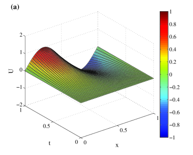
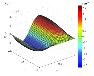
on [0,1]01[0,1]. The ture solution is u(x,t)=t2sin(2πx)𝑢𝑥𝑡superscript𝑡22𝜋𝑥u(x,t)=t^{2}\sin(2\pi x). The algorithm is first run with α=0.8𝛼0.8\alpha=0.8, τ=2.0×10²𝜏2.0superscript102\tau=2.0\times 10^{-2} and M=50𝑀50M=50. In Fig. 3, we plot the approximate solution and a point to point error distribution at t=1𝑡1t=1, where good accuracy is observed. In Table 3, we then report a comparison of e2(M)subscript𝑒2𝑀e_{2}(M), e(M)subscript𝑒𝑀e_{\infty}(M) at t=1𝑡1t=1 between MCTB-DQM and CBCM ref23 , when α=0.3𝛼0.3\alpha=0.3. Here, MCTB-DQM uses τ=5.0×10³𝜏5.0superscript103\tau=5.0\times 10^{-3} while CBCM chooses τ=1.25×10³𝜏1.25superscript103\tau=1.25\times 10^{-3}. As expected, our approach generates the approximate solutions with a better accuracy than those obtained by CBCM.
Refer to caption
Refer to caption
Figure 3: The approximate solution and error distribution at t=1𝑡1t=1 with α=0.8𝛼0.8\alpha=0.8 for Example 6.3
Table 3: A comparison of e2(M)subscript𝑒2𝑀e_{2}(M), e(M)subscript𝑒𝑀e_{\infty}(M) at t=1𝑡1t=1 with α=0.3𝛼0.3\alpha=0.3 for Example 6.3
M𝑀M CBCM ref23 MCTB-DQM
e2(M)subscript𝑒2𝑀e_{2}(M) e(M)subscript𝑒𝑀e_{\infty}(M) e2(M)subscript𝑒2𝑀e_{2}(M) e(M)subscript𝑒𝑀e_{\infty}(M)
8 3.4134e-02 4.8273e-02 9.4300e-03 1.5762e-02
16 8.7334e-03 1.2351e-02 1.1924e-03 2.1670e-03
32 2.1955e-03 3.1048e-03 1.5040e-04 2.8541e-04
64 5.4957e-04 7.7721e-04 1.8925e-05 3.6701e-05
128 1.3739e-04 1.9430e-04 2.3752e-06 4.6559e-06

Example 6.4. We consider a 2D diffusion equation on [1,1]×[1,1]1111[-1,1]\times[-1,1] with εx=εy=1subscript𝜀𝑥subscript𝜀𝑦1\varepsilon_{x}=\varepsilon_{y}=1, which is referred to by Zhai and Feng as a test of a block-centered finite difference method (BCFDM) on nonuniform grids 31 . The forcing function is specified to enforce

u(x,y,t)=(1+t2)tanh(20x)tanh(20y).𝑢𝑥𝑦𝑡1superscript𝑡220𝑥20𝑦u(x,y,t)=(1+t^{2})\tanh(20x)\tanh(20y).

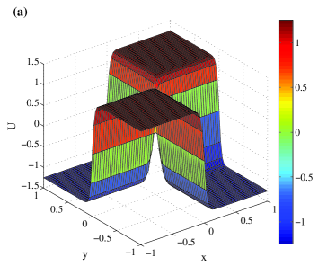
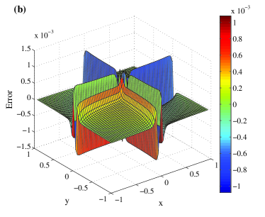
Under τ=1.0×10²𝜏1.0superscript102\tau=1.0\times 10^{-2}, Mx=My=60subscript𝑀𝑥subscript𝑀𝑦60M_{x}=M_{y}=60 and α=0.5𝛼0.5\alpha=0.5, we first plot the approximate solution and a point to point error distribution at t=0.5𝑡0.5t=0.5 in Fig. 4. Then, we compare MCTB-DQM and BCFDM in term of e(Mx,My)subscript𝑒subscript𝑀𝑥subscript𝑀𝑦e_{\infty}(M_{x},M_{y}) at t=0.5𝑡0.5t=0.5 in Table 4. It is obvious that MCTB-DQM produces significantly smaller errors than BCFDM as the grid number increases despite a smaller time stepsize τ=2.5×10³𝜏2.5superscript103\tau=2.5\times 10^{-3} and the nonuniform girds BCFDM adopts; moreover, MCTB-DQM provides more than quadratic rate of convergence for this problem.
Refer to caption
Refer to caption
Figure 4: The approximate solution and error distribution at t=0.5𝑡0.5t=0.5 with α=0.5𝛼0.5\alpha=0.5 for Example 6.4
Table 4: A comparison of e(Mx,My)subscript𝑒subscript𝑀𝑥subscript𝑀𝑦e_{\infty}(M_{x},M_{y}) at t=0.5𝑡0.5t=0.5 with α=0.5𝛼0.5\alpha=0.5 for Example 6.4
Mx,Mysubscript𝑀𝑥subscript𝑀𝑦M_{x},M_{y} BCFDM 31 MCTB-DQM
e(Mx,My)subscript𝑒subscript𝑀𝑥subscript𝑀𝑦e_{\infty}(M_{x},M_{y}) Cov. rate e(Mx,My)subscript𝑒subscript𝑀𝑥subscript𝑀𝑦e_{\infty}(M_{x},M_{y}) Cov. rate
12 8.75e-02 - 3.3376e-01 -
24 2.73e-02 1.68 4.6331e-03 6.1707
48 8.26e-03 1.73 3.4566e-04 3.7446
96 2.24e-03 1.88 1.8605e-05 4.2156
Table 5: The numerical results in term of e2(M)subscript𝑒2𝑀e_{2}(M) at t=0.1𝑡0.1t=0.1 for Example 6.5
α𝛼\alpha Method Real part Imaginary part CPU time
0.2 scheme (LABEL:eq22) 7.4588e-04 7.3396e-04 10.355 (s)
0.5 scheme (LABEL:eq22) 3.9328e-03 3.7620e-03 10.819 (s)
0.8 scheme (LABEL:eq22) 4.5245e-03 4.6714e-03 10.775 (s)
1.0 scheme (LABEL:eq22) 2.2229e-03 2.2153e-03 1.7436 (s)
scheme (24) 8.0954e-04 8.1843e-04 0.1521 (s)
Refer to caption
Refer to caption
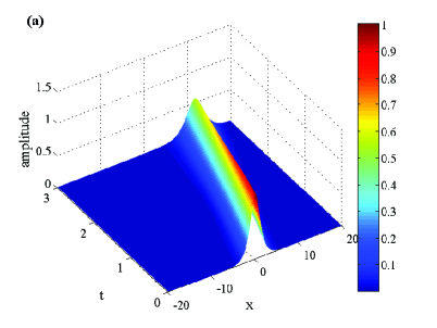
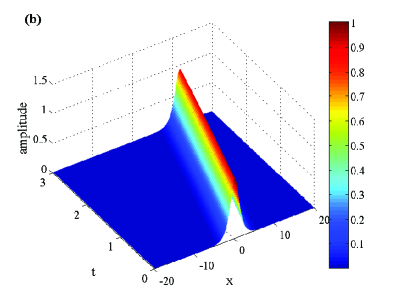
Figure 5: The single soliton propagation for α=0.98𝛼0.98\alpha=0.98, 1.01.01.0 with τ=2.0×10³𝜏2.0superscript103\tau=2.0\times 10^{-3} and M=200𝑀200M=200.

Example 6.5. In this test, we simulate the solitons propagation and collision governed by the following time-fractional nonlinear Schrödinger equation (NLS):

iαutα+2ux2+β|u|2u=0,x(,+),formulae-sequenceisuperscript𝛼𝑢superscript𝑡𝛼superscript2𝑢superscript𝑥2𝛽superscript𝑢2𝑢0𝑥\displaystyle\textrm{i}\frac{\partial^{\alpha}u}{\partial t^{\alpha}}+\frac{\partial^{2}u}{\partial x^{2}}+\beta|u|^{2}u=0,\ \ x\in(-\infty,+\infty),

with i=1i1\textrm{i}=\sqrt{-1} and β𝛽\beta being a real constant, subjected to the initial values of two Gaussian types:

  • (i)

    mobile soliton

    ψ(x)=sech(x)exp(2ix);𝜓𝑥sech𝑥2i𝑥\psi(x)=\textrm{sech}(x)\exp(2\textrm{i}x); (36)
  • (ii)

    double solitons collision

    ψ(x)=j=12sech(xxj)exp(ip(xxj)).𝜓𝑥superscriptsubscript𝑗12sech𝑥subscript𝑥𝑗i𝑝𝑥subscript𝑥𝑗\psi(x)=\sum_{j=1}^{2}\textrm{sech}(x-x_{j})\exp(\textrm{i}p(x-x_{j})). (37)

When α=1𝛼1\alpha=1 and β=2𝛽2\beta=2, the NLS with Eq. (36) has the soliton solution u(x,t)=sech(x4t)exp(i(2x3t))𝑢𝑥𝑡sech𝑥4𝑡i2𝑥3𝑡u(x,t)=\textrm{sech}(x-4t)\exp(\textrm{i}(2x-3t)). As the solutions would generally decay to zero as |x|𝑥|x|\rightarrow\infty, we truncate the system into a bounded interval Ω=[a,b]Ω𝑎𝑏\Omega=[a,b] with a0much-less-than𝑎0a\ll 0 and b0much-greater-than𝑏0b\gg 0, and enforce periodic or homogeneous Dirichlet boundary conditions. Letting u(x,t)=U(x,t)+iV(x,t)𝑢𝑥𝑡𝑈𝑥𝑡i𝑉𝑥𝑡u(x,t)=U(x,t)+\textrm{i}V(x,t). Then, the original equation can be recast as a coupled diffusion system

αUtα+2Vx2+β(U2+V2)V=0,superscript𝛼𝑈superscript𝑡𝛼superscript2𝑉superscript𝑥2𝛽superscript𝑈2superscript𝑉2𝑉0\displaystyle\frac{\partial^{\alpha}U}{\partial t^{\alpha}}+\frac{\partial^{2}V}{\partial x^{2}}+\beta(U^{2}+V^{2})V=0,
αVtα2Ux2β(U2+V2)U=0.superscript𝛼𝑉superscript𝑡𝛼superscript2𝑈superscript𝑥2𝛽superscript𝑈2superscript𝑉2𝑈0\displaystyle\frac{\partial^{\alpha}V}{\partial t^{\alpha}}-\frac{\partial^{2}U}{\partial x^{2}}-\beta(U^{2}+V^{2})U=0.

After applying the scheme (LABEL:eq22), nevertheless, a nonlinear system has to be solved at each time step. In such a case, the Newton’s iteration is utilized to treat it and terminated by reaching a solution with tolerant error 1.0×10121.0superscript10121.0\times 10^{-12} if α=1𝛼1\alpha=1, for which, the Jacobian matrix is

J=(2UVU2+3V23U2V22UV).J2𝑈𝑉superscript𝑈23superscript𝑉23superscript𝑈2superscript𝑉22𝑈𝑉\displaystyle\textbf{J}=\left(\begin{array}[]{cc}2UV&U^{2}+3V^{2}\\ -3U^{2}-V^{2}&-2UV\end{array}\right).

When α1𝛼1\alpha\neq 1, because the analytic solutions still remain unknown and the Newton’s procedure relies heavily on its initial values, we instead employ the trust-region-dogleg algorithm built into Matlab to improve the convergence of iteration. At first, taking τ=2.0×10³𝜏2.0superscript103\tau=2.0\times 10^{-3}, M=100𝑀100M=100, β=2𝛽2\beta=2, and Ω=[10,10]Ω1010\Omega=[-10,10], the mean square errors at t=0.1𝑡0.1t=0.1 with the initial condition (36) for various α𝛼\alpha are reported in Table 5, where the solutions computed by using the coefficients (12) on a very fine time-space lattice, i.e., τ=2.5×10⁴𝜏2.5superscript104\tau=2.5\times 10^{-4}, M=400𝑀400M=400, are adopted as reference solutions (α1𝛼1\alpha\neq 1). As seen from Table 5, our methods are convergent and applicable to nonlinear coupled problems; besides, the scheme (24) is clearly more efficient than (LABEL:eq22) since an extra Newton’s outer loop is avoided. Then, retaking M=200𝑀200M=200 and Ω=[20,20]Ω2020\Omega=[-20,20], we display the evolution of the amplitude of the mobile soliton created by (LABEL:eq22) for α=0.98𝛼0.98\alpha=0.98 and 1.01.01.0 in Fig. 5, respectively. Using the same discrete parameters, we consider the double solitons collision for α=0.96𝛼0.96\alpha=0.96 and 1.01.01.0 with x1=6subscript𝑥16x_{1}=-6, x2=6subscript𝑥26x_{2}=6, and p=±2𝑝plus-or-minus2p=\pm 2 in Fig. 6. It is easily drawn from these figures that the width and height of the solitons have been significantly changed by the fractional derivative. In particular, when α=1𝛼1\alpha=1, a collision of double solitons without any reflection, transmission, trapping and creation of new solitary waves is exhibited, which says that it is elastic, while in fractional cases, the shapes of the solitons may not be retained after they intersect each other.
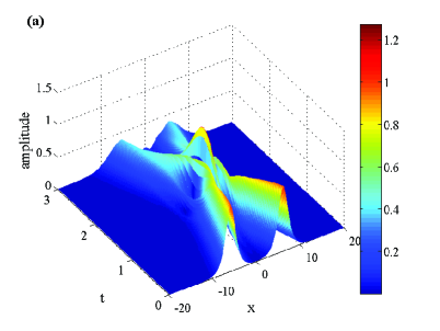
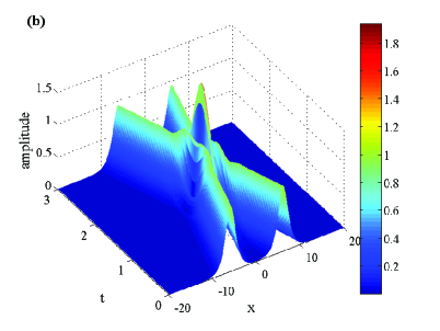
Refer to caption
Refer to caption
Figure 6: The interaction of double solitons for α=0.96𝛼0.96\alpha=0.96, 1.01.01.0 with τ=2.0×10³𝜏2.0superscript103\tau=2.0\times 10^{-3} and M=200𝑀200M=200.

Example 6.6. In this test, we simulate an unsteady propagation of a Gaussian pulse governed by a classical 2D advection-dominated diffusion equation on a square domain [0,2]×[0,2]0202[0,2]\times[0,2] by using the scheme (24), which has been extensively studied ninep02 ; 32 ; 33 ; cirbf00 . The Gaussian pulse solution is expressed as

u(x,y,t)=11+4texp((xκxt0.5)2εx(1+4t)(yκyt0.5)2εy(1+4t)),𝑢𝑥𝑦𝑡114𝑡superscript𝑥subscript𝜅𝑥𝑡0.52subscript𝜀𝑥14𝑡superscript𝑦subscript𝜅𝑦𝑡0.52subscript𝜀𝑦14𝑡u(x,y,t)\!=\!\frac{1}{1+4t}\exp\Bigg{(}-\frac{(x-\!\kappa_{x}t-\!0.5)^{2}}{\varepsilon_{x}(1+4t)}-\frac{(y-\!\kappa_{y}t-\!0.5)^{2}}{\varepsilon_{y}(1+4t)}\Bigg{)},

and the initial Gaussian pulse and boundary values are taken from the pulse solution. Letting κx=κy=0.8subscript𝜅𝑥subscript𝜅𝑦0.8\kappa_{x}=\kappa_{y}=0.8, εx=εy=0.01subscript𝜀𝑥subscript𝜀𝑦0.01\varepsilon_{x}=\varepsilon_{y}=0.01, we display its true solution at t=1.25𝑡1.25t=1.25 with Mx=My=50subscript𝑀𝑥subscript𝑀𝑦50M_{x}=M_{y}=50 and the used lattice points on problem domain in Fig. 7, which describe a pulse centred at (1.5,1.5)1.51.5(1.5,1.5) with a pulse height of 1/6161/6. Using the same grid number together with τ=5.0×10³𝜏5.0superscript103\tau=5.0\times 10^{-3}, we present the contour plots of the approximate solutions at t=0𝑡0t=0, 0.250.250.25, 0.750.750.75, 1.251.251.25 created by MCTB-DQM in Fig. 6. As the graph shows, the pulse is initially centred at (0.5,0.5)0.50.5(0.5,0.5) with a pulse height of 111, then it moves towards a position centred at (1.5,1.5)1.51.5(1.5,1.5); during this process, its width and height appear to be continuously varying as the time goes by. Besides, the last contour plot in Fig. 6 coincides with the true solution plotted in Fig. 7. Retaking τ=6.25×10³𝜏6.25superscript103\tau=6.25\times 10^{-3} and Mx=My=80subscript𝑀𝑥subscript𝑀𝑦80M_{x}=M_{y}=80, we compare our results with those obtained by some previous algorithms as nine-point high-order compact (HOC) schemes ninep02 ; 33 , Peaceman-Rachford ADI scheme (PR-ADI) pr08 , HOC-ADI scheme hoc03 , exponential HOC-ADI scheme (EHOC-ADI) ehoc05 , HOC boundary value method (HOC-BVM) bvm06 , compact integrated RBF ADI method (CIRBF-ADI) cirbf00 , coupled compact integrated RBF ADI method (CCIRBF-ADI) cirbf01 , and the Galerkin FEM combined with the method of characteristics (CGFEM) cgfem07 , at t=1.25𝑡1.25t=1.25 in Table 6. We implement CGFEM on a quasi-uniform triangular mesh with the meshsize 2.5×1022.5superscript1022.5\times 10^{-2} by using both Lagrangian P1 and P2 elements. Also, average absolute errors are added as supplements to evaluate and compare their accuracy. As seen from Table 6, all of these methods are illustrated to be very accurate to capture the Gaussian pulse except the PR-ADI scheme; besides, our method reaches a better accuracy than the others and even shows promise in treating the advection-diffusion equations in the high Péclet number regime.
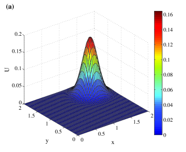
Refer to caption
Refer to caption
Figure 7: The true solution at t=1.25𝑡1.25t=1.25 and spatial lattice points for Example 6.6
[Uncaptioned image]
[Uncaptioned image]
[Uncaptioned image]
Figure 8: The contour plots of Gaussian pulse at t=0𝑡0t=0, 0.250.250.25, 0.750.750.75, 1.251.251.25 with τ=5.0×10³𝜏5.0superscript103\tau=5.0\times 10^{-3} and Mx=My=50subscript𝑀𝑥subscript𝑀𝑦50M_{x}=M_{y}=50.
Table 6: A comparison of global errors at t=1.25𝑡1.25t=1.25 with τ=6.25×10³𝜏6.25superscript103\tau=6.25\times 10^{-3} and Mx=My=80subscript𝑀𝑥subscript𝑀𝑦80M_{x}=M_{y}=80 for Example 6.6.
Method Average Error e2(Mx,My)subscript𝑒2subscript𝑀𝑥subscript𝑀𝑦e_{2}(M_{x},M_{y}) e(Mx,My)subscript𝑒subscript𝑀𝑥subscript𝑀𝑦e_{\infty}(M_{x},M_{y})
CIRBF-ADI cirbf00 6.742e-06 2.197e-05 1.703e-04
CCIRBF-ADI cirbf01 5.989e-06 1.904e-05 1.427e-04
Noye and Tan 33 1.971e-05 1.280e-04 6.509e-04
Kalita et al. ninep02 1.597e-05 1.024e-04 4.477e-04
PR-ADI pr08 3.109e-04 2.025e-03 7.778e-03
HOC-ADI hoc03 9.218e-06 5.931e-05 2.500e-04
EHOC-ADI ehoc05 9.663e-06 6.194e-05 2.664e-04
HOC-BVM bvm06 9.4931e-06 - 2.4766e-04
CGFEM P1 6.3746e-05 1.8849e-04 1.5731e-03
CGFEM P2 1.5667e-05 5.4061e-05 5.8044e-04
MCTB-DQM 9.1512e-07 5.6996e-06 2.2830e-05

Example 6.7. In the last test, we consider the 2D space-fractional equations (LABEL:xz01)-(9) on [0,1]×[0,1]0101[0,1]\times[0,1] with εx=εy=1subscript𝜀𝑥subscript𝜀𝑦1\varepsilon_{x}=\varepsilon_{y}=1, ψ(x,y)=x2(1x)2y2(1y)2𝜓𝑥𝑦superscript𝑥2superscript1𝑥2superscript𝑦2superscript1𝑦2\psi(x,y)=x^{2}(1-x)^{2}y^{2}(1-y)^{2}, and homogeneous boundary values. The source term is manufactured as

f(x,y,t)=etx2(1x)2y2(1y)2𝑓𝑥𝑦𝑡superscript𝑒𝑡superscript𝑥2superscript1𝑥2superscript𝑦2superscript1𝑦2\displaystyle f(x,y,t)=-e^{-t}x^{2}(1-x)^{2}y^{2}(1-y)^{2}
2etx2β1y2(1y)2Γ(3β1)(16x3β1+12x2(3β1)(4β1))2superscript𝑒𝑡superscript𝑥2subscript𝛽1superscript𝑦2superscript1𝑦2Γ3subscript𝛽116𝑥3subscript𝛽112superscript𝑥23subscript𝛽14subscript𝛽1\displaystyle\ -\frac{2e^{-t}x^{2-\beta_{1}}y^{2}(1-y)^{2}}{\Gamma(3-\beta_{1})}\Bigg{(}1-\frac{6x}{3-\beta_{1}}+\frac{12x^{2}}{(3-\beta_{1})(4-\beta_{1})}\Bigg{)}
2etx2(1x)2y2β2Γ(3β2)(16y3β2+12y2(3β2)(4β2))2superscript𝑒𝑡superscript𝑥2superscript1𝑥2superscript𝑦2subscript𝛽2Γ3subscript𝛽216𝑦3subscript𝛽212superscript𝑦23subscript𝛽24subscript𝛽2\displaystyle\ -\frac{2e^{-t}x^{2}(1-x)^{2}y^{2-\beta_{2}}}{\Gamma(3-\beta_{2})}\Bigg{(}1-\frac{6y}{3-\beta_{2}}+\frac{12y^{2}}{(3-\beta_{2})(4-\beta_{2})}\Bigg{)}

to enforce the analytic solution u(x,y,t)=etx2(1x)2y2(1y)2𝑢𝑥𝑦𝑡superscript𝑒𝑡superscript𝑥2superscript1𝑥2superscript𝑦2superscript1𝑦2u(x,y,t)=e^{-t}x^{2}(1-x)^{2}y^{2}(1-y)^{2}. Letting β1=1.1subscript𝛽11.1\beta_{1}=1.1, β2=1.3subscript𝛽21.3\beta_{2}=1.3, and τ=2.5×10⁴𝜏2.5superscript104\tau=2.5\times 10^{-4}, we solve the problem via the FEM proposed by wx05 and MCB-DQM, and compare their numerical results at t=0.2𝑡0.2t=0.2 in Table 7, where the P1 element and structured meshes are adopted. The data indicate that DQ method converges towards the analytic solution as the grid numbers increase and admits slightly better results than FEM. More importantly, the implemental CPU times of MCB-DQM are less than those of FEM, which confirm its computing efficiency.

7 Conclusion

The ADEs are the subjects of active interest in mathematical physics and the related areas of research. In this work, we have proposed an effective DQ method for such equations involving the derivatives of fractional orders in time and space. Its weighted coefficients are calculated by making use of modified CTBs and cubic B-splines as test functions. The stability of DQ method for the time-fractional ADEs in the context of L2subscript𝐿2L_{2}-norm is performed. The theoretical condition required for the stable analysis is numerically surveyed at length. We test the codes on several benchmark problems and the outcomes have demonstrated that it outperforms some of the previously reported algorithms such as BCFDM and FEM in term of overall accuracy and efficiency.

In a linear space, spanned by a set of proper basis functions as B-splines, any function can be represented by a weighted combination of these basis functions. While all basis functions are defined, the function remains unknown because the coefficients on the front of basis functions are still unknown. However, when all basis functions satisfy Eqs. (32)-(33), by virtue of linearity, it can be examined that the objective function satisfies Eqs. (32)-(33) as well. This is the essence of DQ methods, which guarantees their convergence.

Despite the error bounds are difficult to determine, the numerical results illustrate that the spline-based DQ method admits the convergent results for the fractional ADEs. The presented approach can be generalized to the higher-dimensional and other complex model problems arising in material science, structural and fluid mechanics, heat conduction, biomedicine, differential dynamics, and so forth. High computing efficiency, low memory requirement, and the ease of programming are its main advantages.

Acknowledgements.
The authors are very grateful to the reviewers for their valuable comments and suggestions. This research was supported by National Natural Science Foundations of China (Nos.11471262 and 11501450).
Table 7: A comparison of global errors at t=0.2𝑡0.2t=0.2 with τ=2.5×10⁴𝜏2.5superscript104\tau=2.5\times 10^{-4}, β1=1.1subscript𝛽11.1\beta_{1}=1.1, and β2=1.3subscript𝛽21.3\beta_{2}=1.3 for Example 6.7.
Method Mx,Mysubscript𝑀𝑥subscript𝑀𝑦M_{x},\ M_{y} e2(Mx,My)subscript𝑒2subscript𝑀𝑥subscript𝑀𝑦e_{2}(M_{x},M_{y}) Cov. rate e(Mx,My)subscript𝑒subscript𝑀𝑥subscript𝑀𝑦e_{\infty}(M_{x},M_{y}) Cov. rate CPU time
FEM wx05 10 6.5781e-05 - 1.5632e-04 - 63.750(s)
15 3.0082e-05 1.9296 7.2433e-05 1.8972 199.37(s)
20 1.7376e-05 1.9079 4.1321e-05 1.9511 494.98(s)
25 1.1404e-05 1.8872 2.6599e-05 1.9741 1062.7(s)
MCB-DQM​​ 10 5.4217e-05 - 1.4763e-04 - 0.3726(s)
15 2.6606e-05 1.7556 6.9553e-05 1.8562 1.1785(s)
20 1.5559e-05 1.8650 4.0088e-05 1.9153 4.0598(s)
25 1.0207e-05 1.8892 2.6163e-05 1.9124 11.267(s)
{strip}

Appendix: The explicit formulas of the fractional derivatives of cubic B-splines

The fractional derivatives center at x1subscript𝑥1x_{-1}, x0subscript𝑥0x_{0}, and x1subscript𝑥1x_{1}:

Dxβx0RLB1(x)={(1β)(xx0)βΓ(2β)3(xx0)1βΓ(2β)h+6(xx0)2βΓ(3β)h26(xx0)3βΓ(4β)h3,x[x0,x1)(1β)(xx0)βΓ(2β)3(xx0)1βΓ(2β)h+6(xx0)2βΓ(3β)h26(xx0)3βΓ(4β)h3+6(xx1)3βΓ(4β)h3,x[x1,xM]superscriptsubscriptsubscriptsuperscript𝐷𝛽𝑥subscript𝑥0𝑅𝐿subscript𝐵1𝑥cases1𝛽superscript𝑥subscript𝑥0𝛽Γ2𝛽3superscript𝑥subscript𝑥01𝛽Γ2𝛽6superscript𝑥subscript𝑥02𝛽Γ3𝛽superscript26superscript𝑥subscript𝑥03𝛽Γ4𝛽superscript3𝑥subscript𝑥0subscript𝑥11𝛽superscript𝑥subscript𝑥0𝛽Γ2𝛽3superscript𝑥subscript𝑥01𝛽Γ2𝛽6superscript𝑥subscript𝑥02𝛽Γ3𝛽superscript26superscript𝑥subscript𝑥03𝛽Γ4𝛽superscript36superscript𝑥subscript𝑥13𝛽Γ4𝛽superscript3𝑥subscript𝑥1subscript𝑥𝑀\displaystyle{{}^{RL}_{x_{0}}}D^{\beta}_{x}B_{-1}(x)\!=\!\left\{\begin{array}[]{l}\frac{(1-\beta)(x-x_{0})^{-\beta}}{\Gamma(2-\beta)}-\frac{3(x-x_{0})^{1-\beta}}{\Gamma(2-\beta)h}+\frac{6(x-x_{0})^{2-\beta}}{\Gamma(3-\beta)h^{2}}-\frac{6(x-x_{0})^{3-\beta}}{\Gamma(4-\beta)h^{3}},\quad x\in[x_{0},x_{1})\\ \frac{(1-\beta)(x-x_{0})^{-\beta}}{\Gamma(2-\beta)}-\frac{3(x-x_{0})^{1-\beta}}{\Gamma(2-\beta)h}+\frac{6(x-x_{0})^{2-\beta}}{\Gamma(3-\beta)h^{2}}-\frac{6(x-x_{0})^{3-\beta}}{\Gamma(4-\beta)h^{3}}+\frac{6(x-x_{1})^{3-\beta}}{\Gamma(4-\beta)h^{3}},\quad x\in[x_{1},x_{M}]\end{array}\right.
Dxβx0RLB0(x)={4(1β)(xx0)βΓ(2β)12(xx0)2βΓ(3β)h2+18(xx0)3βΓ(4β)h3,x[x0,x1)4(1β)(xx0)βΓ(2β)12(xx0)2βΓ(3β)h2+18(xx0)3βΓ(4β)h324(xx1)3βΓ(4β)h3,x[x1,x2)4(1β)(xx0)βΓ(2β)12(xx0)2βΓ(3β)h2+18(xx0)3βΓ(4β)h324(xx1)3βΓ(4β)h3+6(xx2)3βΓ(4β)h3,x[x2,xM]superscriptsubscriptsubscriptsuperscript𝐷𝛽𝑥subscript𝑥0𝑅𝐿subscript𝐵0𝑥cases41𝛽superscript𝑥subscript𝑥0𝛽Γ2𝛽12superscript𝑥subscript𝑥02𝛽Γ3𝛽superscript218superscript𝑥subscript𝑥03𝛽Γ4𝛽superscript3𝑥subscript𝑥0subscript𝑥141𝛽superscript𝑥subscript𝑥0𝛽Γ2𝛽12superscript𝑥subscript𝑥02𝛽Γ3𝛽superscript218superscript𝑥subscript𝑥03𝛽Γ4𝛽superscript324superscript𝑥subscript𝑥13𝛽Γ4𝛽superscript3𝑥subscript𝑥1subscript𝑥241𝛽superscript𝑥subscript𝑥0𝛽Γ2𝛽12superscript𝑥subscript𝑥02𝛽Γ3𝛽superscript218superscript𝑥subscript𝑥03𝛽Γ4𝛽superscript324superscript𝑥subscript𝑥13𝛽Γ4𝛽superscript36superscript𝑥subscript𝑥23𝛽Γ4𝛽superscript3𝑥subscript𝑥2subscript𝑥𝑀\displaystyle{{}^{RL}_{x_{0}}}D^{\beta}_{x}B_{0}(x)\!=\!\left\{\begin{array}[]{l}\frac{4(1-\beta)(x-x_{0})^{-\beta}}{\Gamma(2-\beta)}-\frac{12(x-x_{0})^{2-\beta}}{\Gamma(3-\beta)h^{2}}+\frac{18(x-x_{0})^{3-\beta}}{\Gamma(4-\beta)h^{3}},\quad x\in[x_{0},x_{1})\\ \frac{4(1-\beta)(x-x_{0})^{-\beta}}{\Gamma(2-\beta)}-\frac{12(x-x_{0})^{2-\beta}}{\Gamma(3-\beta)h^{2}}+\frac{18(x-x_{0})^{3-\beta}}{\Gamma(4-\beta)h^{3}}-\frac{24(x-x_{1})^{3-\beta}}{\Gamma(4-\beta)h^{3}},\quad x\in[x_{1},x_{2})\\ \frac{4(1-\beta)(x-x_{0})^{-\beta}}{\Gamma(2-\beta)}-\frac{12(x-x_{0})^{2-\beta}}{\Gamma(3-\beta)h^{2}}+\frac{18(x-x_{0})^{3-\beta}}{\Gamma(4-\beta)h^{3}}-\frac{24(x-x_{1})^{3-\beta}}{\Gamma(4-\beta)h^{3}}+\frac{6(x-x_{2})^{3-\beta}}{\Gamma(4-\beta)h^{3}},\quad x\in[x_{2},x_{M}]\end{array}\right.
Dxβx0RLB1(x)={(1β)(xx0)βΓ(2β)+3(xx0)1βΓ(2β)h+6(xx0)2βΓ(3β)h218(xx0)3βΓ(4β)h3,x[x0,x1)(1β)(xx0)βΓ(2β)+3(xx0)1βΓ(2β)h+6(xx0)2βΓ(3β)h218(xx0)3βΓ(4β)h3+36(xx1)3βΓ(4β)h3,x[x1,x2)(1β)(xx0)βΓ(2β)+3(xx0)1βΓ(2β)h+6(xx0)2βΓ(3β)h218(xx0)3βΓ(4β)h3+36(xx1)3βΓ(4β)h324(xx2)3βΓ(4β)h3,x[x2,x3)(1β)(xx0)βΓ(2β)+3(xx0)1βΓ(2β)h+6(xx0)2βΓ(3β)h218(xx0)3βΓ(4β)h3+36(xx1)3βΓ(4β)h324(xx2)3βΓ(4β)h3+6(xx3)3βΓ(4β)h3.x[x3,xM]\displaystyle{{}^{RL}_{x_{0}}}D^{\beta}_{x}B_{1}(x)\!=\!\left\{\begin{array}[]{l}\frac{(1-\beta)(x-x_{0})^{-\beta}}{\Gamma(2-\beta)}+\frac{3(x-x_{0})^{1-\beta}}{\Gamma(2-\beta)h}+\frac{6(x-x_{0})^{2-\beta}}{\Gamma(3-\beta)h^{2}}-\frac{18(x-x_{0})^{3-\beta}}{\Gamma(4-\beta)h^{3}},\quad x\in[x_{0},x_{1})\\ \frac{(1-\beta)(x-x_{0})^{-\beta}}{\Gamma(2-\beta)}+\frac{3(x-x_{0})^{1-\beta}}{\Gamma(2-\beta)h}+\frac{6(x-x_{0})^{2-\beta}}{\Gamma(3-\beta)h^{2}}-\frac{18(x-x_{0})^{3-\beta}}{\Gamma(4-\beta)h^{3}}+\frac{36(x-x_{1})^{3-\beta}}{\Gamma(4-\beta)h^{3}},\quad x\in[x_{1},x_{2})\\ \frac{(1-\beta)(x-x_{0})^{-\beta}}{\Gamma(2-\beta)}+\frac{3(x-x_{0})^{1-\beta}}{\Gamma(2-\beta)h}+\frac{6(x-x_{0})^{2-\beta}}{\Gamma(3-\beta)h^{2}}-\frac{18(x-x_{0})^{3-\beta}}{\Gamma(4-\beta)h^{3}}+\frac{36(x-x_{1})^{3-\beta}}{\Gamma(4-\beta)h^{3}}-\frac{24(x-x_{2})^{3-\beta}}{\Gamma(4-\beta)h^{3}},\quad x\in[x_{2},x_{3})\\ \frac{(1-\beta)(x-x_{0})^{-\beta}}{\Gamma(2-\beta)}+\frac{3(x-x_{0})^{1-\beta}}{\Gamma(2-\beta)h}+\frac{6(x-x_{0})^{2-\beta}}{\Gamma(3-\beta)h^{2}}-\frac{18(x-x_{0})^{3-\beta}}{\Gamma(4-\beta)h^{3}}+\frac{36(x-x_{1})^{3-\beta}}{\Gamma(4-\beta)h^{3}}-\frac{24(x-x_{2})^{3-\beta}}{\Gamma(4-\beta)h^{3}}+\frac{6(x-x_{3})^{3-\beta}}{\Gamma(4-\beta)h^{3}}.\quad x\in[x_{3},x_{M}]\end{array}\right.

The fractional derivatives center at xmsubscript𝑥𝑚x_{m} with 2mM+12𝑚𝑀12\leq m\leq M+1:

Dxβx0RLBm(x)={0,x[x0,xm2)6(xxm2)3βΓ(4β)h3,x[xm2,xm1)6(xxm2)3βΓ(4β)h324(xxm1)3βΓ(4β)h3,x[xm1,xm)6(xxm2)3βΓ(4β)h324(xxm1)3βΓ(4β)h3+36(xxm)3βΓ(4β)h3,x[xm,xm+1)6(xxm2)3βΓ(4β)h324(xxm1)3βΓ(4β)h3+36(xxm)3βΓ(4β)h324(xxm+1)3βΓ(4β)h3,x[xm+1,xm+2)6(xxm2)3βΓ(4β)h324(xxm1)3βΓ(4β)h3+36(xxm)3βΓ(4β)h324(xxm+1)3βΓ(4β)h3+6(xxm+2)3βΓ(4β)h3,x[xm+2,xM]superscriptsubscriptsubscriptsuperscript𝐷𝛽𝑥subscript𝑥0𝑅𝐿subscript𝐵𝑚𝑥cases0𝑥subscript𝑥0subscript𝑥𝑚26superscript𝑥subscript𝑥𝑚23𝛽Γ4𝛽superscript3𝑥subscript𝑥𝑚2subscript𝑥𝑚16superscript𝑥subscript𝑥𝑚23𝛽Γ4𝛽superscript324superscript𝑥subscript𝑥𝑚13𝛽Γ4𝛽superscript3𝑥subscript𝑥𝑚1subscript𝑥𝑚6superscript𝑥subscript𝑥𝑚23𝛽Γ4𝛽superscript324superscript𝑥subscript𝑥𝑚13𝛽Γ4𝛽superscript336superscript𝑥subscript𝑥𝑚3𝛽Γ4𝛽superscript3𝑥subscript𝑥𝑚subscript𝑥𝑚16superscript𝑥subscript𝑥𝑚23𝛽Γ4𝛽superscript324superscript𝑥subscript𝑥𝑚13𝛽Γ4𝛽superscript336superscript𝑥subscript𝑥𝑚3𝛽Γ4𝛽superscript324superscript𝑥subscript𝑥𝑚13𝛽Γ4𝛽superscript3𝑥subscript𝑥𝑚1subscript𝑥𝑚26superscript𝑥subscript𝑥𝑚23𝛽Γ4𝛽superscript324superscript𝑥subscript𝑥𝑚13𝛽Γ4𝛽superscript336superscript𝑥subscript𝑥𝑚3𝛽Γ4𝛽superscript324superscript𝑥subscript𝑥𝑚13𝛽Γ4𝛽superscript36superscript𝑥subscript𝑥𝑚23𝛽Γ4𝛽superscript3𝑥subscript𝑥𝑚2subscript𝑥𝑀\displaystyle{{}^{RL}_{x_{0}}}D^{\beta}_{x}B_{m}(x)\!=\!\left\{\begin{array}[]{l}0,\qquad\qquad\qquad\,x\in[x_{0},x_{m-2})\\ \frac{6(x-x_{m-2})^{3-\beta}}{\Gamma(4-\beta)h^{3}},\quad x\in[{x_{m-2}},{x_{m-1}})\\ \frac{6(x-x_{m-2})^{3-\beta}}{\Gamma(4-\beta)h^{3}}-\frac{24(x-x_{m-1})^{3-\beta}}{\Gamma(4-\beta)h^{3}},\quad x\in[{x_{m-1}},{x_{m}})\\ \frac{6(x-x_{m-2})^{3-\beta}}{\Gamma(4-\beta)h^{3}}-\frac{24(x-x_{m-1})^{3-\beta}}{\Gamma(4-\beta)h^{3}}+\frac{36(x-x_{m})^{3-\beta}}{\Gamma(4-\beta)h^{3}},\quad x\in[{x_{m}},{x_{m+1}})\\ \frac{6(x-x_{m-2})^{3-\beta}}{\Gamma(4-\beta)h^{3}}-\frac{24(x-x_{m-1})^{3-\beta}}{\Gamma(4-\beta)h^{3}}+\frac{36(x-x_{m})^{3-\beta}}{\Gamma(4-\beta)h^{3}}-\frac{24(x-x_{m+1})^{3-\beta}}{\Gamma(4-\beta)h^{3}},\quad x\in[{x_{m+1}},{x_{m+2}})\\ \frac{6(x-x_{m-2})^{3-\beta}}{\Gamma(4-\beta)h^{3}}-\frac{24(x-x_{m-1})^{3-\beta}}{\Gamma(4-\beta)h^{3}}+\frac{36(x-x_{m})^{3-\beta}}{\Gamma(4-\beta)h^{3}}-\frac{24(x-x_{m+1})^{3-\beta}}{\Gamma(4-\beta)h^{3}}+\frac{6(x-x_{m+2})^{3-\beta}}{\Gamma(4-\beta)h^{3}},\quad x\in[x_{m+2},x_{M}]\end{array}\right.

which contain Dxβx0RLBM1(x)superscriptsubscriptsubscriptsuperscript𝐷𝛽𝑥subscript𝑥0𝑅𝐿subscript𝐵𝑀1𝑥{{}^{RL}_{x_{0}}}D^{\beta}_{x}B_{M-1}(x), Dxβx0RLBM(x)superscriptsubscriptsubscriptsuperscript𝐷𝛽𝑥subscript𝑥0𝑅𝐿subscript𝐵𝑀𝑥{{}^{RL}_{x_{0}}}D^{\beta}_{x}B_{M}(x), and Dxβx0RLBM+1(x)superscriptsubscriptsubscriptsuperscript𝐷𝛽𝑥subscript𝑥0𝑅𝐿subscript𝐵𝑀1𝑥{{}^{RL}_{x_{0}}}D^{\beta}_{x}B_{M+1}(x) as special cases:

Dxβx0RLBM1(x)={0,x[x0,xM3)6(xxM3)3βΓ(4β)h3,x[xM3,xM2)6(xxM3)3βΓ(4β)h324(xxM2)3βΓ(4β)h3,x[xM2,xM1)6(xxM3)3βΓ(4β)h324(xxM2)3βΓ(4β)h3+36(xxM1)3βΓ(4β)h3,x[xM1,xM]superscriptsubscriptsubscriptsuperscript𝐷𝛽𝑥subscript𝑥0𝑅𝐿subscript𝐵𝑀1𝑥cases0𝑥subscript𝑥0subscript𝑥𝑀36superscript𝑥subscript𝑥𝑀33𝛽Γ4𝛽superscript3𝑥subscript𝑥𝑀3subscript𝑥𝑀26superscript𝑥subscript𝑥𝑀33𝛽Γ4𝛽superscript324superscript𝑥subscript𝑥𝑀23𝛽Γ4𝛽superscript3𝑥subscript𝑥𝑀2subscript𝑥𝑀16superscript𝑥subscript𝑥𝑀33𝛽Γ4𝛽superscript324superscript𝑥subscript𝑥𝑀23𝛽Γ4𝛽superscript336superscript𝑥subscript𝑥𝑀13𝛽Γ4𝛽superscript3𝑥subscript𝑥𝑀1subscript𝑥𝑀\displaystyle{{}^{RL}_{x_{0}}}D^{\beta}_{x}B_{M-1}(x)\!=\!\left\{\begin{array}[]{l}0,\qquad\qquad\qquad\,x\in[x_{0},x_{M-3})\\ \frac{6(x-x_{M-3})^{3-\beta}}{\Gamma(4-\beta)h^{3}},\quad x\in[x_{M-3},x_{M-2})\\ \frac{6(x-x_{M-3})^{3-\beta}}{\Gamma(4-\beta)h^{3}}-\frac{24(x-x_{M-2})^{3-\beta}}{\Gamma(4-\beta)h^{3}},\quad x\in[{x_{M-2}},x_{M-1})\\ \frac{6(x-x_{M-3})^{3-\beta}}{\Gamma(4-\beta)h^{3}}-\frac{24(x-x_{M-2})^{3-\beta}}{\Gamma(4-\beta)h^{3}}+\frac{36(x-x_{M-1})^{3-\beta}}{\Gamma(4-\beta)h^{3}},\quad x\in[x_{M-1},x_{M}]\end{array}\right.
Dxβx0RLBM(x)={0,x[x0,xM2)6(xxM2)3βΓ(4β)h3,x[xM2,xM1)6(xxM2)3βΓ(4β)h324(xxM1)3βΓ(4β)h3,x[xM1,xM]superscriptsubscriptsubscriptsuperscript𝐷𝛽𝑥subscript𝑥0𝑅𝐿subscript𝐵𝑀𝑥cases0𝑥subscript𝑥0subscript𝑥𝑀26superscript𝑥subscript𝑥𝑀23𝛽Γ4𝛽superscript3𝑥subscript𝑥𝑀2subscript𝑥𝑀16superscript𝑥subscript𝑥𝑀23𝛽Γ4𝛽superscript324superscript𝑥subscript𝑥𝑀13𝛽Γ4𝛽superscript3𝑥subscript𝑥𝑀1subscript𝑥𝑀\displaystyle{{}^{RL}_{x_{0}}}D^{\beta}_{x}B_{M}(x)\!=\!\left\{\begin{array}[]{l}0,\quad x\in[x_{0},x_{M-2})\\ \frac{6(x-x_{M-2})^{3-\beta}}{\Gamma(4-\beta)h^{3}},\quad x\in[x_{M-2},x_{M-1})\\ \frac{6(x-x_{M-2})^{3-\beta}}{\Gamma(4-\beta)h^{3}}-\frac{24(x-x_{M-1})^{3-\beta}}{\Gamma(4-\beta)h^{3}},\quad x\in[x_{M-1},x_{M}]\end{array}\right.
Dxβx0RLBM+1(x)={0,x[x0,xM1)6(xxM1)3βΓ(4β)h3.x[xM1,xM]\displaystyle{{}^{RL}_{x_{0}}}D^{\beta}_{x}B_{M+1}(x)\!=\!\left\{\begin{array}[]{l}0,\quad x\in[x_{0},x_{M-1})\\ \frac{6(x-x_{M-1})^{3-\beta}}{\Gamma(4-\beta)h^{3}}.\quad x\in[x_{M-1},x_{M}]\end{array}\right.

References

  • (1) Abbas, M., Majid, A.A., Ismail, A.I.M., Rashid, A.: The application of cubic trigonometric B-spline to the numerical solution of the hyperbolic problems. Appl. Math. Comput. 239, 74–88 (2014)
  • (2) Bellman, R., Casti, J.: Differential quadrature and long-term integration. J. Math. Anal. Appl. 34(2), 235–238 (1971)
  • (3) Bhrawy, A., Zaky, M.: A fractional-order Jacobi Tau method for a class of time-fractional PDEs with variable coefficients. Math. Method Appl. Sci. 39(7), 1765–1779 (2016)
  • (4) Chen, M.H., Deng, W.H.: Fourth order difference approximations for space Riemann-Liouville derivatives based on weighted and shifted Lubich difference operators. Commun. Comput. Phys. 16(2), 516–540 (2014)
  • (5) Chen, Y.M., Wu, Y.B., Cui, Y.H., Wang, Z.Z., Jin, D.M.: Wavelet method for a class of fractional convection-diffusion equation with variable coefficients. J. Comput. Sci. 1(3), 146–149 (2010)
  • (6) Cui, M.R.: A high-order compact exponential scheme for the fractional convection-diffusion equation. J. Comput. Appl. Math. 255, 404–416 (2014)
  • (7) Dehghan, M., Mohebbi, A.: High-order compact boundary value method for the solution of unsteady convection–diffusion problems. Math. Comput. Simulat. 79(3), 683–699 (2008)
  • (8) Douglas, Jr., J., Russell, T.F.: Numerical methods for convection-dominated diffusion problems based on combining the method of characteristics with finite element or finite difference procedures. SIAM J. Numer. Anal. 19(5), 871–885 (1982)
  • (9) Esmaeili, S., Garrappa, R.: A pseudo-spectral scheme for the approximate solution of a time-fractional diffusion equation. Int. J. Comput. Math. 92(5), 980–994 (2015)
  • (10) Gao, G.H., Sun, H.W.: Three-point combined compact alternating direction implicit difference schemes for two-dimensional time-fractional advection-diffusion equations. Commun. Comput. Phys. 17(2), 487–509 (2015)
  • (11) Heydari, M.H.: Wavelets Galerkin method for the fractional subdiffusion equation. J. Comput. Nonlinear Dynam. 11(6), 061,014 (2016)
  • (12) Hosseini, S.M., Ghaffari, R.: Polynomial and nonpolynomial spline methods for fractional sub-diffusion equations. Appl. Math. Model. 38(14), 3554–3566 (2014)
  • (13) Huang, C.B., Yu, X.J., Wang, C., Li, Z.Z., An, N.: A numerical method based on fully discrete direct discontinuous Galerkin method for the time fractional diffusion equation. Appl. Math. Comput. 264, 483–492 (2015)
  • (14) Izadkhah, M.M., Saberi-Nadjafi, J.: Gegenbauer spectral method for time-fractional convection-diffusion equations with variable coefficients. Math. Method Appl. Sci. 38(15), 3183–3194 (2015)
  • (15) Jia, J.H., Wang, H.: A fast finite volume method for conservative space-fractional diffusion equations in convex domains. J. Comput. Phys. 310, 63–84 (2016)
  • (16) Ji, C.C., Sun, Z.Z.: A high-order compact finite difference scheme for the fractional sub-diffusion equation. J. Sci. Comput. 64(3), 959–985 (2015)
  • (17) Jiang, Y.J., Ma, J.T.: High-order finite element methods for time-fractional partial differential equations. J. Comput. Appl. Math. 235(11), 3285–3290 (2011)
  • (18) Jin, B.T., Lazarov, R., Zhou, Z.: Error estimates for a semidiscrete finite element method for fractional order parabolic equations. SIAM J. Numer. Anal. 51(1), 445–466 (2013)
  • (19) Kalita, J.C., Dalal, D.C., Dass, A.K.: A class of higher order compact schemes for the unsteady two-dimensional convection–diffusion equation with variable convection coefficients. Int. J. Numer. Meth. Fluids 38(12), 1111–1131 (2002)
  • (20) Karaa, S., Zhang, J.: High order ADI method for solving unsteady convection–diffusion problems. J. Comput. Phys. 198(1), 1–9 (2004)
  • (21) Kilbas, A.A., Srivastava, H.M., Trujillo, J.J.: Theory and Applications of Fractional Differential Equations. Elsevier B. V., Amsterdam (2006)
  • (22) Laub, A.J.: Matrix Analysis For Scientists & Engineers. Society for Industrial and Applied Mathematics, Philadelphia, PA (2005)
  • (23) Lin, Y.M., Xu, C.J.: Finite difference/spectral approximations for the time-fractional diffusion equation. J. Comput. Phys. 225(2), 1533–1552 (2007)
  • (24) Liu, Q., Gu, Y.T., Zhuang, P., Liu, F., Nie, Y.F.: An implicit RBF meshless approach for time fractional diffusion equations. Comput. Mech. 48(1), 1–12 (2011)
  • (25) Luo, W.H., Huang, T.Z., Wu, G.C., Gu, X.M.: Quadratic spline collocation method for the time fractional subdiffusion equation. Appl. Math. Comput. 276, 252–265 (2016)
  • (26) Mittal, R.C., Jain, R.K.: Numerical solutions of nonlinear Burgers’ equation with modified cubic B-splines collocation method. Appl. Math. Comput. 218(15), 7839-7855 (2012)
  • (27) Ma, Y.B., Sun, C.P., Haake, D.A., Churchill, B.M., Ho, C.M.: A high-order alternating direction implicit method for the unsteady convection-dominated diffusion problem. Int. J. Numer. Meth. Fluids 70(6), 703–712 (2012)
  • (28) Meerschaert, M.M., Scheffler, H.P., Tadjeran, C.: Finite difference methods for two-dimensional fractional dispersion equation. J. Comput. Phys. 211(1), 249–261 (2006)
  • (29) Mainardi, F.: Fractals and Fractional Calculus Continuum Mechanics. Springer, Verlag (1997)
  • (30) Nazir, T., Abbas, M., Ismail, A.I.M., Majid, A.A., Rashid, A.: The numerical solution of advection-diffusion problems using new cubic trigonometric B-splines approach. Appl. Math. Model. 40(7-8), 4586–4611 (2016)
  • (31) Noye, B.J., Tan, H.H.: Finite difference methods for solving the two-dimensional advection-diffusion equation. Int. J. Numer. Meth. Fluids 9(1), 75–98 (1989)
  • (32) Peaceman, D.W., Rachford, Jr., H.H.: The numerical solution of parabolic and elliptic differential equations. J. Soc. Indust. Appl. Math. 3(1), 28–41 (1955)
  • (33) Pirkhedri, A., Javadi, H.H.S.: Solving the time-fractional diffusion equation via Sinc-Haar collocation method. Appl. Math. Comput. 257, 317–326 (2015)
  • (34) Podlubny, I.: Fractional Differential Equations. Academic Press, San Diego, CA (1999)
  • (35) Razminia, K., Razminia, A., Baleanu, D.: Investigation of the fractional diffusion equation based on generalized integral quadrature technique. Appl. Math. Model. 39(1), 86–98 (2015)
  • (36) Roop, J.P.: Computational aspects of FEM approximation of fractional advection dispersion equations onbounded domains in 2superscript2\mathbb{R}^{2}. J. Comput. Appl. Math. 193(1), 243–268 (2006)
  • (37) Saadatmandi, A., Dehghan, M., Azizi, M.R.: The Sinc-Legendre collocation method for a class of fractional convection-diffusion equations with variable coefficients. Commun. Nonlinear Sci. Numer. Simul. 17(11), 4125–4136 (2012)
  • (38) Sayevand, K., Yazdani, A., Arjang, F.: Cubic B-spline collocation method and its application for anomalous fractional diffusion equations in transport dynamic systems. J. Vib. Control 22(9), 2173–2186 (2016)
  • (39) Shirzadi, A., Ling, L., Abbasbandy, S.: Meshless simulations of the two-dimensional fractional-time convection-diffusion-reaction equations. Eng. Anal. Bound. Elem. 36(11), 1522–1527 (2012)
  • (40) Shlesinger, M.F., West, B.J., Klafter, J.: Lévy dynamics of enhanced diffusion: Application to turbulence. Phys. Rev. Lett. 58(11), 1100–1103 (1987)
  • (41) Shu, C., Richards, B.E.: Application of generalized differential quadrature to solve two-dimensional incompressible Navier-Stokes equations. Int. J. Numer. Meth. Fluids 15(7), 791–798 (1992)
  • (42) Tomasiello, S.: Stability and accuracy of the iterative differential quadrature method. Int. J. Numer. Methods Eng. 58(9), 1277-1296 (2003)
  • (43) Tomasiello, S.: Numerical stability of DQ solutions of wave problems. Numer. Algor. 57(3), 289-312 (2011)
  • (44) Tian, W.Y., Zhou, H., Deng, W.H.: A class of second order difference approximations for solving space fractional diffusion equations. Math. Comp. 84(294), 1703-1727 (2015)
  • (45) Thai-Quang, N., Mai-Duy, N., Tran, C.-D., Tran-Cong, T.: High-order alternating direction implicit method based on compact integrated-RBF approximations for unsteady/steady convection-diffusion equations. CMES Comput. Model. Eng. Sci. 89(3), 189–220 (2012)
  • (46) Tian, Z.F., Ge, Y.B.: A fourth-order compact ADI method for solving two-dimensional unsteady convection–diffusion problems. J. Comput. Appl. Math. 198(1), 268–286 (2007)
  • (47) Tien, C.M.T., Thai-Quang, N., Mai-Duy, N., Tran, C.-D., Tran-Cong, T.: A three-point coupled compact integrated RBF scheme for second-order differential problems. CMES Comput. Model. Eng. Sci. 104(6), 425–469 (2015)
  • (48) Uddin, M., Haq, S.: RBFs approximation method for time fractional partial differential equations. Commun. Nonlinear Sci. Numer. Simul. 16(11), 4208–4214 (2011)
  • (49) Walz, G.: Identities for trigonometric B-splines with an application to curve design. BIT 37(1), 189–201 (1997)
  • (50) Yang, X.H., Zhang, H.X., Xu, D.: Orthogonal spline collocation method for the two-dimensional fractional sub-diffusion equation. J. Comput. Phys. 256, 824–837 (2014)
  • (51) Zaslavsky, G.M., Stevens, D., Weitzner, H.: Self-similar transport in incomplete chaos. Phys. Rev. E. 48(3), 1683–1694 (1993)
  • (52) Zhu, X.G., Nie, Y.F., Wang, J.G., Yuan, Z.B.: A numerical approach for the Riesz space-fractional Fisher’ equation in two-dimensions. Int. J. Comput. Math. 94(2), 296-315 (2017)
  • (53) Zeng, F.H., Li, C.P., Liu, F.W., Turner, I.: The use of finite difference/element approaches for solving the time-fractional subdiffusion equation. SIAM J. Sci. Comput. 35(6), A2976–A3000 (2013)
  • (54) Zeng, F.H., Liu, F.W., Li, C.P., Burrage, K., Turner, I., Anh, V.: A Crank-Nicolson ADI spectral method for a two-dimensional Riesz space fractional nonlinear reaction-diffusion equation. SIAM J. Numer. Anal. 52(6), 2599-2622 (2014)
  • (55) Zhai, S.Y., Feng, X.L.: A block-centered finite-difference method for the time-fractional diffusion equation on nonuniform grids. Numer. Heat Transf., Part B Fundam. 69(3), 217–233 (2016)
  • (56) Zhou, F.Y., Xu, X.Y.: The third kind Chebyshev wavelets collocation method for solving the time-fractional convection diffusion equations with variable coefficients. Appl. Math. Comput. 280, 11–29 (2016)
  • (57) Zhuang, P.H., Liu, F.W.: Implicit difference approximation for the time fractional diffusion equation. J. Appl. Math. & Computing 22(3), 87–99 (2006)