Efficient Branching Cascaded Regression
for Face Alignment under Significant Head Rotation

Abstract

Despite much interest in face alignment in recent years, the large majority of work has focused on near-frontal faces. Algorithms typically break down on profile faces, or are too slow for real-time applications. In this work we propose an efficient approach to face alignment that can handle $180$ degrees of head rotation in a unified way (e.g., without resorting to view-based models) using 2D training data. The foundation of our approach is cascaded shape regression (CSR), which has emerged recently as the leading strategy. We propose a generalization of conventional CSRs that we call branching cascaded regression (BCR). Conventional CSRs are single-track; that is, they progress from one cascade level to the next in a straight line, with each regressor attempting to fit the entire dataset. We instead split the regression problem into two or more simpler ones after each cascade level. Intuitively, each regressor can then operate on a simpler objective function (i.e., with fewer conflicting gradient directions). Within the BCR framework, we model and infer pose-related landmark visibility and face shape simultaneously using Structured Point Distribution Models (SPDMs). We propose to learn task-specific feature mapping functions that are adaptive to landmark visibility, and that use SPDM parameters as regression targets instead of 2D landmark coordinates. Additionally, we introduce a new in-the-wild dataset of profile faces to validate our approach.

1 Introduction

There has been significant research interest in face alignment in recent years, which has resulted in impressive advances in speed and robustness on challenging in-the-wild faces. However, relatively little work (with the exception of a few, e.g. [32]) has been done to handle the full range of head poses encountered in the real world. The large majority of face alignment algorithms focus on near fronto-parallel faces, and break down on profile faces. Handling the full range of head poses is challenging because:

• The 2D shapes of profile faces and frontal faces are significantly different.

• Many landmarks become self-occluded on profile faces.

• Algorithms must contend with greater background noise on profile faces, as most conventional landmarks (e.g., nose tip, lip corners) are not surrounded by the face.

A straightforward approach to large head pose variation is to employ view-based models and choose the result that achieves the best match [8, 40]. However, because head pose is continuous, problems arise at the transition points between models (e.g., $45$ degrees), and employing many view-specific models is inefficient. Nonlinear statistical models (e.g., kernel methods [29] or mixture models [9, 19, 38]) have been proposed to deal with large head pose variation. However, these methods are too slow for real-time applications. Another strategy is to employ a full 3D model of the face [1, 5, 6, 15, 25], but publicly available training data are limited, and algorithms still tend to focus on near fronto-parallel faces [5, 6].

Figure 1: Our branching cascaded regression (BCR) algorithm can handle faces with a wide variety of poses, including full profile.

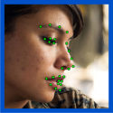We propose an approach to face alignment that can handle $180$ degrees of head rotation angle in a unified way (e.g., without resorting to view-based models) using 2D training data and linear shape models. The foundation of our approach is cascaded shape regression, which has emerged recently as the leading strategy [4, 7, 12, 20, 27, 31, 32, 33, 34, 37]. Cascaded shape regressors (CSRs) are computationally efficient and the core idea is elegant. CSRs are purely discriminative, which means they can capitalize on large and diverse training datasets to perform robust face alignment in the wild. However, we observe two key limitations with the conventional formulation of CSRs:

Limitation 1:

They assume that all landmarks are visible, which is problematic for profile faces.

Limitation 2:

They are local algorithms, and they are likely to average conflicting gradient directions [34], which is especially problematic when they are applied to face collections with large head pose variation.

We address the first limitation by incorporating visibility into the regression. Specifically, we use global structured point distribution models (SPDM) [28] to represent both shape variation and landmark visibility in a unified way, and we train regressors to predict SPDM parameters. SPDMs extend traditional point distribution models (PDMs) [10] by appending a “structure” vector (indicating whether each landmark is visible or not) to the set of shape parameters, and then constructing a combined linear model of shape and landmark visibility. This strategy separates us from the recent trend in face alignment of modeling shape nonparametrically (e.g., [4, 7, 20, 27, 32, 33, 34, 37]). We argue that PDMs have several desirable qualities:

• There are far fewer parameters to optimize, which results in a smaller (and faster to apply) set of regression coefficients.

• All landmarks are optimized simultaneously.

• When learned via PCA, they generalize well to unfamiliar faces.

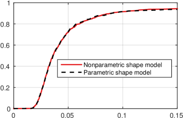
In fact, we show empirically in Figure 4 that there are no significant differences in accuracy and robustness between parametric and nonparametric shape models when used within otherwise identical systems.

We address the second limitation by introducing a branching cascaded regression framework for face alignment. Conventional CSRs are single-track; that is, they progress from one cascade level to the next in a straight line, with each regressor attempting to fit the entire dataset. We instead split the regression problem into two or more simpler ones after each cascade level. Intuitively, each regressor can then operate on a simpler objective function (i.e., with fewer conflicting gradient directions). Our approach is inspired by Xiong and De la Torre [34] who introduced the concept of “domains of homogeneous descent” to define their Global Supervised Descent Method (GSDM). Their algorithm selects a single-path CSR from a library of CSRs, each trained on a different region of the objective function domain, based on the result from the previous frame in a video. In contrast, at runtime our algorithm chooses which branch to take, and thus which sequence of regressors to apply, based on the current test image. Note that the method in [34] reverts to a conventional CSR on single images.

Most CSRs use off-the-shelf feature mapping functions (most commonly SIFT [23]) to produce feature descriptors from the image. Instead, we are inspired by the work of Ren et al. [27] who showed that learned feature mapping functions can be both extremely computationally efficient at runtime, and produce features that are task-specific. In [27], they used regression random forests [3, 11] to induce local binary features that predict landmark updates. We propose to instead use regression random forests to induce local binary features that predict ideal SPDM parameter updates (i.e., for predicting both face shape and landmark visibility simultaneously) and to produce feature descriptors that are adaptive to landmark visibility.

To summarize, we make the following contributions:

1. Branching cascaded regression: We propose to divide the objective function domain after each cascaded regression level, which results in simpler regression problem at each subsequent cascade level.

2. Profile-to-profile faces: The proposed algorithm retains the state-of-the-art speed and accuracy of recent algorithms while handling a much wider range of head poses, including full profile faces with significant self-occlusion.

3. Self-occlusion prediction: To the best of our knowledge, we are the first to employ SPDMs to predict both shape and landmark visibility within a cascaded shape regression framework.

4. Nonparametric vs. parametric: We show empirically (Figure 4) that there is virtually no difference in accuracy between parametric and nonparametric shape models when used within otherwise identical systems on challenging faces.

5. Competitive results on challenging datasets: The proposed approach is competitive with recent state-of-the-art methods on challenging frontal and near-frontal in-the-wild faces, and it produces excellent results on faces with significant non-frontal head pose.

6. New in-the-wild dataset: We have assembled and annotated a challenging dataset of in-the-wild profile faces from the Web to validate different parts of our algorithm and to promote future research in this area.

2 Related Work

Face alignment has a rich history in computer vision. We forgo an extensive overview here due to space limitations and focus on the most relevant work.

Shape regression approaches have recently come to dominate the face alignment landscape [4, 7, 5, 12, 18, 20, 22, 27, 31, 32, 33, 35]. Due to the complex relationships between image appearance and face shape updates, finding the true face shape in one step is difficult. Different strategies have been proposed for this problem, including trying multiple initializations and choosing the best result [4, 7], and performing a coarse-to-fine search [39]. Another strategy, which we employ, is to split the regression problem into multiple iterations (i.e., a cascaded shape regressor (CSR)) and re-compute “shape-indexed” features [7, 12] at each stage. This latter approach is perhaps best exemplified by the Supervised Descent Method (SDM) [33].

Conventional CSRs are single-track; that is, they progress from one cascade level to the next in a straight line, with each regressor attempting to fit the entire dataset. The problem with this strategy is that the objective function includes many conflicting gradient directions, especially when faces with a wide range of poses are included in the dataset. Xiong and De la Torre [34] proposed the Global Supervised Descent Method (GSDM) to address this problem. GSDM splits the objective function into regions of similar gradient directions and constructs a separate single-track CSR for each region. This results in a set of parallel, independent CSRs. When used for face alignment, GSDM is restricted to video because it uses the result from the previous frame to select which CSR to use for the current frame. GSDM reverts to conventional CSR (e.g., SDM [33]) on single images. Instead, we introduce branching into the cascaded shape regression, which works on single images. During training, we split the regression problem into two or more simpler ones after each cascade level, as described in Section 3. This creates a tree-like cascade of shape regressors. At runtime our algorithm adaptively chooses which branch to take, and thus which sequence of regressors to apply, based on the current test image.

CSR-based methods can be divided into two categories: those that use off-the-shelf feature mapping functions like SIFT [23] (e.g., [31, 33, 34]), and those that learn feature mapping functions (e.g., using ensembles of regression trees [20, 22, 27]). Learned feature mapping functions are task-specific, and are extremely computationally efficient at runtime when operating on simple pixel-differences [20, 27]. We use ensembles of regression trees in our approach to induce pixel-difference features correlated with our regression targets. Unlike [27], we novelly construct random regression forests with SPDM coefficients as targets (Section 3) instead of 2D offsets.

Recent work [33, 34, 32], including those that learn feature mapping functions [7, 20, 27], have primarily used the 2D landmark coordinates directly as the regression targets. Instead we employ a PCA-based shape model and use the ideal shape parameter updates as regression targets. Parametric PCA-based models have several desirable qualities: they are very well studied, they require far fewer parameters than nonparametric shape models, they allow all landmarks to be optimized simultaneously, and they generalize well to unfamiliar faces. Tzimiropoulos showed that PCA-based 2D shape models are very competitive with nonparametric ones [31]. We show in Figure 4 that, empirically, there are no significant differences in accuracy and robustness between parametric and nonparametric shape models when used within otherwise identical systems.

Work that addresses significant head pose variation includes view-based models [8, 40], nonlinear statistical models (e.g., kernel methods [29] or mixture models [9, 19, 38]), and 3D shape models [1, 5, 6, 15, 18, 25, 36]. View-based models are straightforward, but require a separate model for each viewpoint, which is inefficient, and problems can arise at midpoints between models. A key trait of our method is that it generates smoothly varying results across a wide range of viewpoints and facial expressions. View-based methods, including tree-structured face detectors [16], generally partition the training set in a discontinuous ad hoc way. In contrast, we partition training faces into overlapping sets in a principled way using PCA. Our method is much faster than view-based methods, which typically compute and score multiple candidate results for each face.

Nonlinear statistical models tend to be too slow for real-time applications. One practical problem with 3D models is that publicly available training data are limited, and most 3D algorithms focus on either easier in-the-lab face datasets [1, 5, 6, 25] and/or near fronto-parallel faces [5, 6, 36]. Another interesting approach is dense 3D face alignment and reconstruction (e.g., [17] and its predecessors), although results suggest that test faces must still be near-frontal.

Until very recently, most research on landmark occlusion has focused on near-frontal faces [4, 37]. The only cue is appearance (face shape is generally uncorrelated), and the presence of occluders is arbitrary. We instead focus on the more tractable problem of estimating occlusion due solely to head pose, which is highly correlated with 2D face shape. We capitalize on this fact by modeling shape and visibility simultaneously using SPDMs [28], as described in Section 3. Note that the original SPDM authors did not propose using SPDMs in this way.

Very recently, researchers have considered the problem of locating landmarks in faces with significant head rotation and occlusion within the CSR framework. Wu and Ji [32] proposed an approach for estimating arbitrary landmark visibility. Inference of landmark visibility with their model is nontrivial, and they used Monte Carlo approximation, which is relatively slow. Instead, we estimate pose-related landmark visibility in a simpler and much faster way. Like our approach, their shape regressors take landmark visibility into account.

Jourabloo and Liu [18] proposed learning a cascaded coupled regressor where, at each cascade level, they learn two regressors: one to estimate parametric 3D shape updates and one to estimate the parameters of a weak perspective model. They estimate landmark visibility indirectly by first estimating the surface normal of each landmark, and then labeling landmarks with negative $z$ coordinates as invisible. In this work, we incorporate pose-related landmark visibility into our model in a unified way, which allows our algorithm to estimate shape and landmark visibility simultaneously. Like previous CSRs, [18] and [32] are single-path, whereas our algorithm chooses the cascade path at runtime.

3 Our Approach

We beginning with a brief overview of Structured Point Distribution Models (SPDMs) [28], followed by a description of our approach.

3.1 Modeling Landmark Visibility with SPDMs

To build an SPDM we first build a Point Distribution Model (PDM) [10]. PDMs model a set of $n$ shapes $\mathbf{S}=[\mathbf{s}_{1},\cdots,\mathbf{s}_{n}]$ using a linear combination of shape bases $\mathbf{B}_{\mathbf{s}}$ plus the mean shape $\mathbf{\mu}_{\mathbf{s}}$:

$$\hat{\mathbf{S}}=\mathbf{\mu}_{\mathbf{s}}+\mathbf{B}_{\mathbf{s}}\mathbf{p}_{\mathbf{s}},\ \ \ \ \ \mathbf{S}\approx\hat{\mathbf{S}},$$ (1)

where $\mathbf{p}_{\mathbf{s}}$ contains the reconstruction parameters; $\mathbf{\mu}_{\mathbf{s}}$, $\mathbf{B}_{\mathbf{s}}$, and $\mathbf{p}_{\mathbf{s}}$ are computed from $\mathbf{S}$ via PCA.

Missing landmarks in $\mathbf{S}$ must be imputed in order to compute $\mathbf{B}_{\mathbf{s}}$ and $\mathbf{p}_{\mathbf{s}}$. Several imputation strategies exist, but we employ Iterated PCA as described in [28]. The missing landmarks in $\mathbf{S}$ are initialized using mean value imputation, i.e., $s_{i}=\hat{s}_{i}=\mu_{i}$, where $i$ indexes missing landmarks. We then set the number of bases to $m=1$ and cycle between computing $\{\mathbf{\mu}_{\mathbf{S}}$, $\mathbf{B}_{\mathbf{s},m}$, $\mathbf{p}_{\mathbf{s},m}\}$ and setting $s_{i}=\hat{s}_{i}$ for all $i$ until convergence. $m$ is then incremented by $1$ and the process is repeated starting with the previous result. We inspect the imputed results after each loop and continue incrementing $m$ until we see no further improvement. We note that imputed landmarks need not be perfect since their visibility will be set to zero later. Once imputation is complete, we can compute $\mathbf{p}_{\mathbf{s}}$ in the usual way.

Prior to PCA, the shapes in $\mathbf{S}$ are aligned using Procrustes Analysis to remove variations due to global face rotation, translation, and scale. To incorporate these variations back into the model, we append four additional basis vectors to $\mathbf{B}_{\mathbf{s},m}$, one for rotation, one for x-translation, one for y-translation, and one for scale, as described in Section 4.2.1 of [24], and re-orthonormalize.

We augment each shape with a binary “structure” vector $\mathbf{v}$ that indicates whether each landmark is visible ($1$) or not ($0$). PCA on $\mathbf{V}=[\mathbf{v}_{1},\cdots,\mathbf{v}_{n}]$ gives a matrix $\mathbf{B}_{\mathbf{v}}$ of visibility bases and a matrix $\mathbf{p}_{\mathbf{v}}$ of continuous landmark visibility parameters. The training shapes can then be represented by a combined set of parameters:

$$\mathbf{p}=\left[\begin{array}[]{c}\mathbf{p}_{\mathbf{s}}\\ \mathbf{p}_{\mathbf{v}}\end{array}\right].$$ (2)

Finally, a combined model of shape and visibility is constructed by performing PCA once more on the combined parameters: $\mathbf{p}=\mathbf{C}\mathbf{q}$, where $\mathbf{C}$ expresses correlations between shape and visibility, and $\mathbf{q}$ is a new parameter space. Note that it is important to first shift and scale $\mathbf{p}_{\mathbf{s}}$ so that its elements lie in the same range as $\mathbf{p}_{\mathbf{v}}$. See [28] for more details.

3.2 Overview

We first give a brief overview of our approach and then present the technical details of each step. Our branching cascaded regressor (BCR) is a binary tree that takes a face image $I$ and a rough initial shape estimate $\mathbf{s}^{0}$ as input, and produces a final shape estimate $\mathbf{s}^{T}$ as output. Initially, all landmarks are assumed to be visible (i.e., $\mathbf{v}=\mathbf{1}$). $\mathbf{s}$ and $\mathbf{v}$ are progressively updated as the input face traverses the tree. At runtime, each BCR node performs two tasks: (1) a shape and landmark visibility update followed by (2) a binary classification of the input face. Depending on the classifier’s output, the face is sent to either the left child or the right child for the next cascade level. Each child node represents a different mode of regression targets. The classifier aims to send the input face to the child node that will best predict its shape.

3.3 Shape and Landmark Visibility Regression

The shape and visibility update at cascade level $t$ in BCR node $k$ is performed by $\mathbf{R}^{t,k}$. We omit $k$ below for simplicity, but it is important to note that each BCR node has its own shape regressor and SPDM. Each BCR node models a subset of similar training faces, which allows each shape regressor and SPDM to be much simpler (fewer parameters) than a single global model. The input to regressor $t$ is a feature descriptor $\mathbf{d}(I,\mathbf{s})$ that captures the local appearance in image $I$ relative to shape $\mathbf{s}$. The output is an updated shape and visibility estimate:

$$\Delta\mathbf{q}^{t} = \mathbf{R}^{t}\mathbf{d}^{t}(I,\mathbf{s}^{t-1})$$ (3)

$$\mathbf{q}^{t} = \mathbf{q}^{t-1}+\Delta\mathbf{q}^{t}$$ (4)

$$\left[\begin{array}[]{c}\mathbf{p}_{\mathbf{s}}^{t}\\ \mathbf{p}_{\mathbf{v}}^{t}\end{array}\right] = \mathbf{C}^{t}\mathbf{q}^{t}$$ (7)

$$\mathbf{s}^{t} = \mathbf{\mu}_{\mathbf{s}}^{t}+\mathbf{B}_{\mathbf{s}}^{t}\mathbf{p}_{\mathbf{s}}^{t}$$ (8)

$$\mathbf{v}^{t} = \mathbf{\mu}_{\mathbf{v}}^{t}+\mathbf{B}_{\mathbf{v}}^{t}\mathbf{p}_{\mathbf{v}}^{t}$$ (9)

Note that $\mathbf{C}$, $\mathbf{B}_{\mathbf{s}}$, and $\mathbf{B}_{\mathbf{v}}$ are specific to each $\{t,k\}$, and so we recompute $\mathbf{q}^{t-1}$ from $\mathbf{s}^{t-1}$ and $\mathbf{v}^{t-1}$ at each level before computing $\mathbf{q}^{t}$:

$$\mathbf{p}_{\mathbf{s}}^{t-1} = {\mathbf{B}_{\mathbf{s}}^{t}}^{\mathsf{T}}(\mathbf{s}^{t-1}-\mathbf{\mu}_{\mathbf{s}}^{t})$$ (10)

$$\mathbf{p}_{\mathbf{v}}^{t-1} = {\mathbf{B}_{\mathbf{v}}^{t}}^{\mathsf{T}}(\mathbf{v}^{t-1}-\mathbf{\mu}_{\mathbf{v}}^{t})$$ (11)

$$\mathbf{q}^{t-1} = {\mathbf{C}^{t}}^{\mathsf{T}}\left[\begin{array}[]{c}\mathbf{p}_{\mathbf{s}}^{t-1}\\ \mathbf{p}_{\mathbf{v}}^{t-1}\end{array}\right]$$ (14)

Each $\mathbf{R}^{t}$ is computed offline by solving the following ridge regression problem:

$$\operatornamewithlimits{argmin}_{\mathbf{R}^{t}}\sum_{i\in N_{t}}\|\Delta\hat{\mathbf{q}}_{i}^{t}-\mathbf{R}^{t}\mathbf{d}^{t}(I_{i},\mathbf{s}^{t-1})\|_{2}^{2}+\lambda\|\mathbf{R}^{t}\|_{2}^{2},$$ (15)

where $\Delta\hat{\mathbf{q}}_{i}^{t}$ is the ideal parameter update for face $i$ and $N_{t}$ are the training faces that belong to the current BCR node. Ridge regression (i.e., the second regularization term) is necessary because $\mathbf{d}^{t}(I,\mathbf{s})$ is very high dimensional (see Section 3.5) and substantial overfitting would result without it [27].

3.4 Branching

Figure 2: Two faces generated by varying the first dimension of our combined shape and landmark visibility model in the first level of the cascade. Note that yaw head rotation is naturally encoded, and the visibility of landmarks shifts smoothly as they rotate toward being occluded.

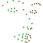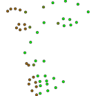
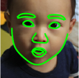
During training, the training examples traverse the BCR much like test faces do. After learning $\mathbf{R}^{t,k}$ in each node, the training examples are partitioned into two overlapping sets, one for each child. The goal is to cluster the training examples into the two most significant modes of regression targets. Intuitively, this gives each child node a regression problem with a simpler objective function. Specifically, we perform dimensionality reduction on the ideal shape and landmark visibility updates via PCA, project the data onto the first (most dominant) subspace dimension, and partition the training set along that dimension. This is equivalent to partitioning along the first dimension of $\Delta\hat{\mathbf{q}}_{i}^{t}$ in Eq. (15). Figure 2 shows two shapes generated by varying this first mode, which naturally encodes both yaw head rotation and pose-related landmark visibility.

We train an L2-regularized linear SVM [13] to predict partition labels from feature descriptors $\mathbf{d}(I,\mathbf{s}^{t-1})$. At test time, our algorithm determines which direction to branch based on the SVM output:

$$y^{t}={\mathbf{w^{t}}}^{\mathsf{T}}\mathbf{d}^{t}(I,\mathbf{s}^{t-1})+b^{t},$$ (16)

(e.g., $y<0$ results in a left child traversal).

Due to image noise, poor initialization, etc., mistakes are inevitable, especially near the decision boundary. Therefore, we retain a sizable fraction of the most difficult-to-classify training faces in each child node that belong to the other branch. This way, if test faces branch incorrectly, subsequent regressors will be general enough to handle them. In our implementation we simply send all training examples down both branches, and throw away the easiest-to-classify $1/3$ that belong to the other branch. In the first node, for example, this results in a $99.5\%$ recall rate for training instances.

3.5 Learning Feature Mapping Functions

In training, each $\mathbf{d}^{t}(I,\mathbf{s})$ is learned separately for each BCR node prior to learning each $\mathbf{R}^{t}$. $\mathbf{d}^{t}$ is composed of many local independent feature mapping functions: $\mathbf{d}^{t}=[d_{1}^{t},\cdots,d_{M}^{t}]$.

We use an ensemble of regression trees [3] to learn each $d_{m}^{t}$ according to [27], with several key differences. First, instead of using the 2D landmark coordinates as regression targets, we use SPDM parameters. Second, instead of allocating trees uniformly across landmarks, we allocate them proportionally to the mean visibility of each landmark in the training data associated with each BCR node. For BCR nodes in which profile faces dominate, for example, the result is an ensemble of trees that emphasize visible landmarks. Third, we train the split nodes of each tree in a different way.

To train each split node, our algorithm first chooses one dimension of $\Delta\hat{\mathbf{q}}_{i}^{t}$. The choice is random, but weighted, where the weight is proportional to the amount of variance that each dimension of $\Delta\hat{\mathbf{q}}_{i}^{t}$ encodes. This emphasizes the most significant modes of variation in the SPDM. We then test $F=500$ random pixel-difference features [27] and select the one that gives rise to maximum variance reduction in the chosen dimension of $\Delta\hat{\mathbf{q}}_{i}^{t}$.

Figure 3: Selected qualitative results on Helen (columns 1 & 2), IBUG (columns 3 & 4), 300-W Fullset (columns 5 & 6), and our new Flickr-Profile dataset (columns 7 & 8). Columns 5 - 8 were generated using our full model and include pose-related landmark visibility estimation. Notice that the red landmarks are correctly labeled as occluded in columns 7 & 8. Please see our supplementary material for additional results. Best viewed electronically in color.

4 Results and Discussion

4.1 Datasets

Multi-PIE [14] is an extensive in-the-lab dataset that includes annotations on profile faces. We use it to train our most general model, which can handle both frontal and profile faces. Additional annotations on Multi-PIE profile faces were provided by [40]. One limitation of Multi-PIE is that all profile landmark annotations are on neutral-expression faces.

Helen (194 landmarks) [21] is a dataset of 2330 high-resolution in-the-wild face images. Most faces are near-frontal, but other challenges are significant, including exaggerated facial expressions, and diversity of subjects.

300 Faces in-the-wild Challenge (300-W) (68 landmarks) [30] is a collection of in-the-wild datasets that were re-annotated with landmarks consistent with Multi-PIE. We closely followed the training and testing procedures described in previous work [39] and used the prescribed face detector results provided by 300-W for initialization. “Common Subset” includes LFPW [2] and Helen, “Challenging Subset” is the iBUG subset, and “Fullset” is the union of the three. We note that “inter-ocular distance” is defined by 300-W as the distance between the outer eye corners.

FERET [26] is an older dataset that includes neutral-expression profile faces against uniform backgrounds. Wu and Ji [32] recently added landmark annotations to $465$ of the profile faces, which allows us to quantitatively compare our results with theirs.

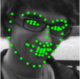
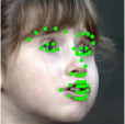
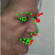
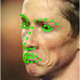
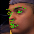
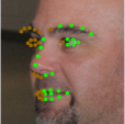
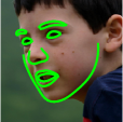
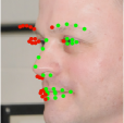
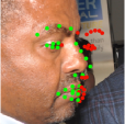
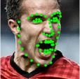
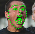
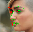
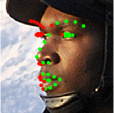
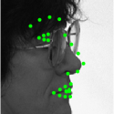
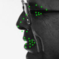
Flickr-Profile is a new in-the-wild dataset that we assembled to validate our approach. Specifically, we collected public domain images from Flickr depicting 170 unique profile faces. We annotated the visible portion of the non-jawline landmarks according to the Multi-PIE mark-up. Images in Flickr-Profile include a variety of challenging illumination conditions, resolutions, noise levels, etc., as shown in Figure 3.

4.2 Comparison on Popular in-the-wild Datasets

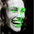
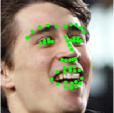
Few recent methods handle both frontal and profile faces with the same model, which limits our ability to evaluate the most general version of our algorithm with recent work. Therefore, we first demonstrate that our method is competitive in a more conventional setting (e.g., with no pose-related landmark occlusion). Specifically, we report averaged errors on Helen and 300-W datasets in Table 1. Note that, during training, we assume that all landmarks are visible for these datasets. Our method performs favorably compared to state-of-the-art methods, achieving the lowest errors in both datasets.

4.3 Comparison on Images with Large Head Rotation

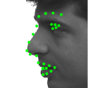
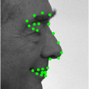
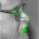
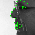
In Figure 6 we compare our results on FERET with [32], [40], and [36]. The curves for [32], [40], and [36] were taken directly from [32]. Like [32], we use Multi-PIE, LFPW, and Helen to train our model for testing on FERET, and we similarly use half the distance between the eye and mouth corner points to normalize each mean error. We see that our results compare favorably.

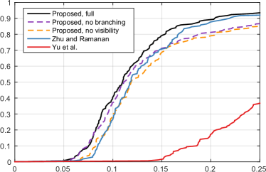
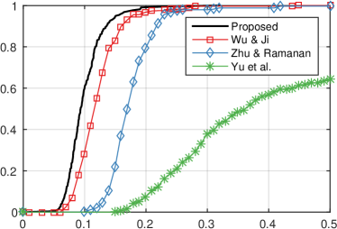
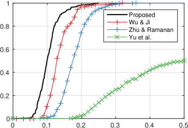
In Figure 5 we validate our algorithm on Flickr-Profile and compare with two other baseline algorithms. We ran the executables from [40] and [36] to generate the plots in Figure 5. Our full algorithm performs well compared to both. To initialize [36], we scaled, translated, and rotated a mean face shape on top of the ground truth points. We ran the code from [40] using their slowest (seconds to minutes per frame), but most accurate model. In Figure 5 we also compare the accuracy of our full model with our model without landmark visibility estimation, and our model without branching. We see that both are required to achieve the best performance on profile faces using general models.

4.4 Implementation Details and Runtime

For all experiments, we use $600$ regression trees with a maximum depth of $6$ for our feature mapping functions, and all of our BCRs have $4$ cascade levels. Like previous work, we augment the training datasets by sampling multiple initializations for each image. Like [20, 27], our algorithm is very fast, although our experimental MATLAB implementation is not. It runs at about $15$ FPS.

Fraction of test faces
	Average normalized error

Figure 4: Comparison between two simplified version of our algorithm, identical except for the shape models used. The nonparametric version updates 2D landmark coordinates directly, while the parametric version updates PDM shape parameters. We see that accuracy is almost identical.

Fraction of test faces
	Average normalized error

Figure 5: Results on Flickr-Profile faces. We see that our proposed algorithm produces more accurate results when branching and landmark visibility estimation are included.

(a) Our five worst-fitting results on FERET					(b) Result from [32]

Fraction of test faces		Fraction of test faces
	Average normalized error		Average normalized error
	(c) Left profile		(d) Right profile

Figure 6: Results on profile faces from the FERET database [26]. (a) The five worst-fitting results from our proposed algorithm. (b) The single worse-fitting result as reported by Wu and Ji [32]. (c)-(d) Cumulative error distribution (CED) curves on profile faces. The CED curves of Wu & Ji [32], Zhu & Ramanan [40], and Yu et al. [36] are reproduced here directly from [32] for comparison. We see that the results from our proposed algorithm are significantly more accurate than recent state-of-the-art methods.

	Helen	300-W Dataset
	(194 landmarks)	(68 landmarks)
Method		Common	Challenging	Fullset
		Subset	Subset
Zhu & Ramanan [40]	-	8.22	18.33	10.20
DRMF [1]	-	6.65	19.79	9.22
ESR [8]	5.70	5.28	17.00	7.58
RCPR [5]	6.50	6.18	17.26	8.35
SDM [33]	5.85	5.60	15.40	7.52
ERT [20]	-	-	-	6.40
LBF [27]	5.41	4.95	11.98	6.32
LBF fast [27]	5.80	5.38	15.50	7.37
CFSS [39]	4.74	4.73	9.98	5.76
CFSS practical [39]	4.84	4.79	10.92	5.99
Lee et al. [22]	-	-	-	5.71
Wu & Ji [32]	-	-	11.52	-
Ours	5.74	5.18	13.26	6.76

Table 1: Averaged normalized error values on popular near-frontal face datasets as reported in the literature. Note that our results are comparable to LBF (on which our approach is based), which is competative with the state of the art. In conjunction with Figures 5 and 6, these results demonstrate that our approach can handle profile faces without sacrificing accuracy on near-frontal faces.

5 Conclusion and Future Work

In this work, we have proposed a novel way to augment cascaded shape regression. Specifically, we proposed branching cascaded regressors for face alignment, in which the algorithm chooses which sequences of regressors to apply adaptively. To deal with pose-related landmark visibility, we incorporated SPDMs into the cascaded regression framework, and showed empirically that nonparametric shape models are no better than parametric ones. Using our approach, we demonstrated state-of-the-art accuracy on challenging datasets, including those with full-profile faces. We hope our work inspires others to address the problem of face alignment on faces in-the-wild with arbitrary head rotation. In particular, additional public datasets are needed for training and testing.

6 Acknowlegements

This work was supported in part by the U.S. Department of Transportation Federal Highway Administration DTFH61-14-C-00011.

References

- [1] T. Baltrusaitis, P. Robinson, and L. Morency. 3D constrained local model for rigid and non-rigid facial tracking. In CVPR, 2012.
- [2] P. N. Belhumeur, D. W. Jacobs, D. J. Kriegman, and N. Kumar. Localizing parts of faces using a consensus of exemplars. In The 24th IEEE Conference on Computer Vision and Pattern Recognition (CVPR), June 2011.
- [3] L. Breiman. Random forests. Machine learning, 45:5–32, 2001.
- [4] X. P. Burgos-Artizzu, P. Perona, and P. Dollár. Robust face landmark estimation under occlusion. In ICCV, 2013.
- [5] C. Cao, Y. Weng, S. Lin, and K. Zhou. 3D shape regression for real-time facial animation. ACM Transactions on Graphics (TOG), 32(4):41:1–41:10, July 2013.
- [6] X. Cao, Q. Hou, and K. Zhou. Displacing dynamic expression regression for real-time facial tracking and animation. ACM Transactions on Graphics (TOG), 33(4), 2014.
- [7] X. Cao, Y. Wei, F. Wen, and J. Sun. Face alignment by explicit shape regression. In CVPR, 2012.
- [8] T. Cootes, K. Walker, and C. Taylor. View-based active appearance models. In IEEE FG, 2015.
- [9] T. F. Cootes and C. Taylor. A mixture model for representing shape variation. In BMVC, 1999.
- [10] T. F. Cootes, C. J. Taylor, D. H. Cooper, and J. Graham. Active shape models – their training and application. Computer Vision and Image Understanding, 61(1):38–59, 1995.
- [11] A. Criminisi and J. Shotton. Regression forests. In A. Criminisi and J. Shotton, editors, Decision Forests for Computer Vision and Medical Image Analysis, Advances in Computer Vision and Pattern Recognition, pages 47–58. Springer London, 2013.
- [12] P. Dollár, P. Welinder, and P. Perona. Cascaded pose regression. In CVPR, 2010.
- [13] R.-E. Fan, K.-W. Chang, C.-J. Hsieh, X.-R. Wang, and C.-J. Lin. LIBLINEAR: A library for large linear classification. Journal of Machine Learning Research, 9:1871–1874, 2008.
- [14] R. Gross, I. Matthews, J. Cohn, T. Kanade, and S. Baker. Multi-PIE. Image and Vision Computing, 28(5):807–813, May 2010.
- [15] L. Gu and T. Kanade. 3D alignment of face in a single image. In CVPR, 2006.
- [16] C. Huang, H. Ai, Y. Li, and S. Lao. High-performance rotation invariant multiview face detection. PAMI, 2007.
- [17] L. A. Jeni, J. F. Cohn, and T. Kanade. Dense 3D face alignment from 2d videos in real-time. In FG, 2015.
- [18] A. Jourabloo and X. Liu. Pose-invariant 3d face alignment. In ICCV, 2015.
- [19] A. Kanaujia, Y. Huang, and D. Metaxas. Tracking facial features using mixture of point distribution models. In Computer Vision, Graphics and Image Processing, volume 4338 of Lecture Notes in Computer Science, pages 492–503. Springer Berlin Heidelberg, 2006.
- [20] V. Kazemi and J. Sullivan. One millisecond face alignment with an ensemble of regression trees. In CVPR, 2014.
- [21] V. Le, J. Brandt, Z. Lin, L. D. Bourdev, and T. S. Huang. Interactive facial feature localization. In ECCV, 2012.
- [22] D. Lee, H. Park, and C. D. Yoo. Face alignment using cascade gaussian process regression trees. In CVPR, 2015.
- [23] D. G. Lowe. Distinctive image features from scale-invariant keypoints. International Journal of Computer Vision (IJCV), 60(2):91–110, 2004.
- [24] I. Matthews and S. Baker. Active Appearance Models revisited. International Journal of Computer Vision, 60(2):135 – 164, November 2004.
- [25] I. Matthews, J. Xiao, and S. Baker. 2D vs. 3D deformable face models: Representational power, construction, and real-time fitting. International Journal of Computer Vision, 75(1):93–113, 2007.
- [26] P. J. Phillips, H. Moon, P. Rauss, and S. A. Rizvi. The FERET evaluation methodology for face-recognition algorithms. In CVPR, 1997.
- [27] S. Ren, X. Cao, Y. Wei, and J. Sun. Face alignment at 3000 fps via regressing local binary features. In CVPR, 2014.
- [28] M. Rogers and J. Graham. Structured point distribution models: Modelling intermittently present features. In BMVA, 2001.
- [29] S. Romdhani, S. Gong, and A. Psarrou. A multi-view nonlinear active shape model using kernel PCA. In BMVC, 1999.
- [30] C. Sagonas, G. Tzimiropoulos, S. Zafeiriou, and M. Pantic. A semi-automatic methodology for facial landmark annotation. In CVPR-W, 2013.
- [31] G. Tzimiropoulos. Project-out cascaded regression with an application to face alignment. In CVPR, 2015.
- [32] Y. Wu and Q. Ji. Robust facial landmark detection under significant head poses and occlusion. In ICCV, 2014.
- [33] X. Xiong and F. De la Torre. Supervised descent method and its applications to face alignment. In CVPR, 2013.
- [34] X. Xiong and F. De la Torre. Global supervised descent method. In CVPR, 2015.
- [35] H. Yang and I. Patras. Mirror, mirror on the wall, tell me, is the error small? In CVPR, 2015.
- [36] X. Yu, J. Huang, S. Zhang, W. Yan, and D. Metaxas. Pose-free facial landmark fitting via optimized part mixtures and cascaded deformable shape model. In ICCV, 2013.
- [37] X. Yu, Z. Lin, J. Brandt, and D. N. Metaxas. Consensus of regression for occlusion-robust facial feature localization. In ECCV, 2014.
- [38] Y. Zhou, W. Zhang, X. Tang, and H. Shum. A bayesian mixture model for multi-view face alignment. In CVPR, 2005.
- [39] S. Zhu, C. Li, C. C. Loy, and X. Tang. Face alignment by coarse-to-fine shape searching. In CVPR, 2015.
- [40] X. Zhu and D. Ramanan. Face detection, pose estimation, and landmark localization in the wild. In Computer Vision and Pattern Recognition (CVPR), 2012 IEEE Conference on, 2012.