Updated fit to three neutrino mixing: exploring the accelerator–reactor complementarity
Abstract
We perform a combined fit to global neutrino oscillation data available as of fall 2016 in the scenario of three-neutrino oscillations and present updated allowed ranges of the six oscillation parameters. We discuss the differences arising between the consistent combination of the data samples from accelerator and reactor experiments compared to partial combinations. We quantify the confidence in the determination of the less precisely known parameters , , and the neutrino mass ordering by performing a Monte Carlo study of the long baseline accelerator and reactor data. We find that the sensitivity to the mass ordering and the octant is below . Maximal mixing is allowed at slightly more than 90% CL. The best fit for the CP violating phase is around , CP conservation is allowed at slightly above , and values of are disfavored at around 99% CL for normal ordering and higher CL for inverted ordering.
Keywords:
neutrino oscillations, solar and atmospheric neutrinos1 Introduction
Experiments measuring the flavor composition of solar neutrinos, atmospheric neutrinos, neutrinos produced in nuclear reactors and in accelerators have established that lepton flavor is not conserved in neutrino propagation, but it oscillates with a wavelength depending on distance and energy, because neutrinos are massive and the mass states are admixtures of the flavor states Pontecorvo:1967fh ; Gribov:1968kq , see Ref. GonzalezGarcia:2007ib for an overview.
With the exception of a set of unconfirmed “hints” of possible eV scale mass states (see Ref. Giunti:2015wnd for a recent review), all the oscillation signatures can be explained with the three flavor neutrinos (, , ), which can be expressed as quantum superpositions of three massive states () with masses . This implies the presence of a leptonic mixing matrix in the weak charged current interactions Maki:1962mu ; Kobayashi:1973fv which can be parametrized as:
| (1) |
where and . The angles can be taken without loss of generality to lie in the first quadrant, , and the phase . Here is a diagonal matrix which is the identity if neutrinos are Dirac fermions and it contains two additional phases if they are Majorana fermions, and plays no role in neutrino oscillations Bilenky:1980cx ; Langacker:1986jv . In this convention there are two non-equivalent orderings for the neutrino masses which can be chosen to be: normal ordering (NO) with , and inverted ordering (IO) with . Furthermore the data shows a relatively large hierarchy between the mass splittings, with . In this work we follow the convention introduced in Ref. Gonzalez-Garcia:2014bfa and present our results in terms of the variable , with for NO and for IO. Hence, for NO and for IO, i.e., it corresponds to the mass splitting with the largest absolute value.
In this article, we present an up-to-date (as of fall 2016) global analysis of neutrino data in the framework of three-neutrino oscillations. Alternative recent global fits have been presented in Refs. Capozzi:2016rtj ; Forero:2014bxa . With current data from the accelerator long-baseline experiments MINOS, T2K, NOA and modern reactor experiments like Daya-Bay, RENO, and Double-Chooz, their complementarity anticipated more than a decade ago Minakata:2002jv ; Huber:2003pm ; Huber:2004ug has become a reality, and the combined analysis starts to show some sensitivity to subtle effects like the octant or the phase (though still at low statistical significance).
The outline of the paper is as follows: In Sec. 2.1 we describe the data samples included in our analysis (see also Appendix A for a schematic list). The presently allowed ranges of the six oscillation parameters are given in Sec. 2.2 assuming that follows a -distribution, while Sec. 2.3 contains the corresponding measures of CP violation in terms of the leptonic Jarlskog invariant and the leptonic unitarity triangle. Deviations from the Gaussian approximation of the confidence intervals for and and the confidence level for the mass ordering determination are quantified in Sec. 4. Several issues appearing in the present analysis are discussed in Sec. 3, in particular about the consistent combination of results from long baseline accelerator experiments with reactors results, now that both provide comparable precision in the determination of the relevant mass-squared difference. We also give the updated status on the ongoing tension in the determination from solar experiments versus KamLAND, and comment on the stand-by in the analysis of the Super-Kamiokande atmospheric data. Sec. 5 contains the summary of our results.
2 Global analysis: determination of oscillation parameters
2.1 Data samples analyzed
In the analysis of solar neutrino data we consider the total rates from the radiochemical experiments Chlorine Cleveland:1998nv , Gallex/GNO Kaether:2010ag and SAGE Abdurashitov:2009tn , the results for the four phases of Super-Kamiokande Hosaka:2005um ; Cravens:2008aa ; Abe:2010hy ; sksol:nakano2016 ; sksol:ichep2016 , the data of the three phases of SNO included in the form of the parametrization presented in Aharmim:2011vm , and the results of both Phase-I and Phase-II of Borexino Bellini:2011rx ; Bellini:2008mr ; Bellini:2014uqa .
Results from long baseline (LBL) accelerator experiments include the final energy distribution of events from MINOS Adamson:2013whj ; Adamson:2013ue in and disappearance and and appearance channels, as well as the latest energy spectrum for T2K in the same four channels t2k:ichep2016 ; t2k:susy2016 and for NOA on the disappearance and appearance neutrino modes nova:nu2016 .
Data samples on disappearance from reactor include the full results of the long baseline reactor data in KamLAND Gando:2010aa , as well as the results from medium baseline reactor experiments from CHOOZ Apollonio:1999ae and Palo Verde Piepke:2002ju . Concerning running experiments we include the latest spectral data from Double-Chooz dc:moriond2016 and Daya-Bay db:nu2016 , while for RENO we use the total rates obtained with their largest data sample corresponding to 800 days of data-taking reno:nu2014 .
In the analysis of the reactor data, the unoscillated reactor flux is determined as described in Kopp:2013vaa by including in the fit the results from short baseline reactor data (RSBL) from ILL Kwon:1981ua , Gösgen Zacek:1986cu , Krasnoyarsk Vidyakin:1987ue ; Vidyakin:1994ut , ROVNO88 Afonin:1988gx , ROVNO4 Kuvshinnikov:1990ry , Bugey3 Declais:1994su , Bugey4 Declais:1994ma , and SRP Greenwood:1996pb .
For the analysis of atmospheric neutrinos we include the results from IceCube/DeepCore 3-year data Aartsen:2014yll .
2.2 Results: oscillation parameters
The results of our standard analysis are presented in Figs. 1 and 2 where we show projections of the allowed six-dimensional parameter space.111 tables from the global analysis corresponding to all 1-dimensional and 2-dimensional projections are available for download at the NuFIT website nufit . In all cases when including reactor experiments we leave the normalization of reactor fluxes free and include data from short-baseline (less than 100 m) reactor experiments. In our previous analysis Gonzalez-Garcia:2014bfa ; GonzalezGarcia:2012sz we studied the impact of this choice versus that of fixing the reactor fluxes to the prediction of the latest calculations Mueller:2011nm ; Huber:2011wv ; Mention:2011rk . As expected, the overall description is better when the flux normalization is fitted against the data. We find which is just another way to quantify the well-known short baseline reactor anomaly to be . However, the difference in the resulting parameter determination (in particular for ) between these two reactor flux normalization choices has become marginal, since data from the reactor experiments with near detectors such as Daya-Bay, RENO and Double-Chooz (for which the near-far comparison allows for flux-normalization independent analysis) is now dominant. Consequently, in what follows we show only the projections for our standard choice with fitted reactor flux normalization.
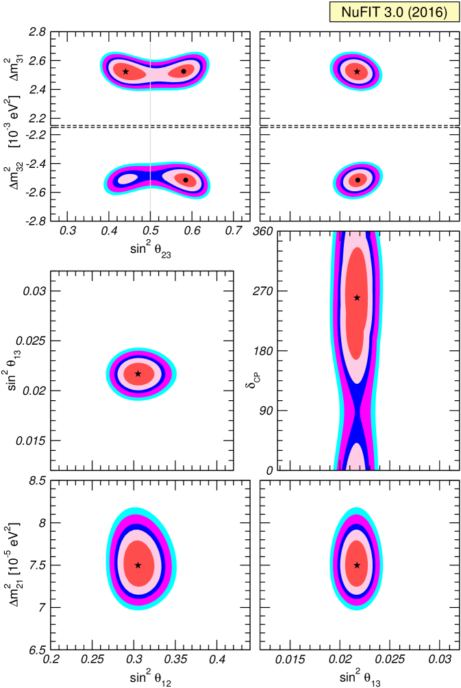
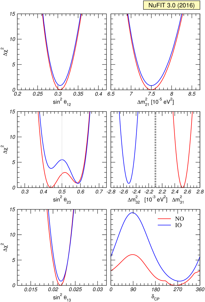
The best fit values and the derived ranges for the six parameters at the () level are given in Tab. 1. For each parameter the ranges are obtained after marginalizing with respect to the other parameters222In this paper we use the term “marginalization” over a given parameter as synonym for minimizing the function with respect to that parameter. and under the assumption that follows a distribution. Hence the () ranges are given by the condition (9). It is known that because of its periodic nature and the presence of parameter degeneracies the statistical distribution of the marginalized for and (and consequently the corresponding CL intervals) may be modified Schwetz:2006md ; Blennow:2014sja . In Sec. 4 we will discuss and quantify these effects.
In Tab. 1 we list the results for three scenarios. In the first and second columns we assume that the ordering of the neutrino mass states is known a priori to be Normal or Inverted, respectively, so the ranges of all parameters are defined with respect to the minimum in the given scenario. In the third column we make no assumptions on the ordering, so in this case the ranges of the parameters are defined with respect to the global minimum (which corresponds to Normal Ordering) and are obtained marginalizing also over the ordering. For this third case we only give the ranges. In this case the range of is composed of two disconnected intervals, one containing the absolute minimum (NO) and the other the secondary local minimum (IO).
| Normal Ordering (best fit) | Inverted Ordering () | Any Ordering | |||
|---|---|---|---|---|---|
| bfp | range | bfp | range | range | |
Defining the relative precision of a parameter by , where () is the upper (lower) bound on a parameter at the level, we read relative precision of 14% (), 32% (), 11% (), 14% () and 9% () for the various oscillation parameters.
2.3 Results: leptonic mixing matrix and CP violation
From the global analysis described in the previous section and following the procedure outlined in Ref. GonzalezGarcia:2003qf one can derive the ranges on the magnitude of the elements of the leptonic mixing matrix:
| (2) |
Note that there are strong correlations between the elements due to the unitary constraint.
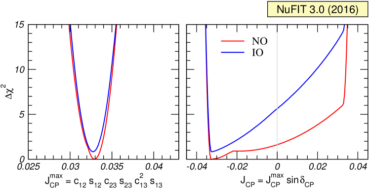
The present status of the determination of leptonic CP violation is illustrated in Fig. 3. In the left panel we show the dependence of of the global analysis on the Jarlskog invariant which gives a convention-independent measure of CP violation Jarlskog:1985ht , defined as usual by:
| (3) |
where we have used the parametrization in Eq. (1). Thus the determination of the mixing angles yields at present a maximum allowed CP violation
| (4) |
at () for both orderings. The preference of the present data for non-zero implies a best fit value , which is favored over CP conservation with . These numbers can be compared with the size of the Jarlskog invariant in the quark sector, which is determined to be PDG .
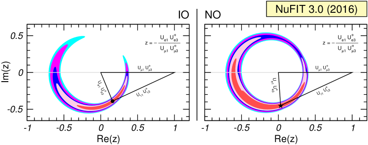
In Fig. 4 we recast the allowed regions for the leptonic mixing matrix in terms of one leptonic unitarity triangle. Since in the analysis is unitary by construction, any given pair of rows or columns can be used to define a triangle in the complex plane. In the figure we show the triangle corresponding to the unitarity conditions on the first and third columns which is the equivalent to the one usually shown for the quark sector. In this figure the absence of CP violation implies a flat triangle, i.e., . As can be seen, for NO the horizontal axis crosses the allowed region, which for 2 dof corresponds to . This is consistent with the present preference for CP violation, mentioned above. We will comment on the statistical interpretation of this number in Sec. 4.
3 Issues in present analysis
The fit results in the previous section provide a statistically satisfactory description of all the neutrino oscillation data considered. There are however some issues in the determination of some of the parameters which, although not of statistical significance at present, deserve some attention.
3.1 Status of in solar experiments versus KamLAND
The analyses of the solar experiments and of KamLAND give the dominant contribution to the determination of and . It has been a result of global analyses for several years already, that the value of preferred by KamLAND is somewhat higher than the one from solar experiments. This tension arises from a combination of two effects which have not changed significantly over the last lustrum: a) the well-known fact that none of the 8B measurements performed by SNO, SK and Borexino shows any evidence of the low energy spectrum turn-up expected in the standard LMA-MSW Wolfenstein:1977ue ; Mikheev:1986gs solution for the value of favored by KamLAND; b) the observation of a non-vanishing day-night asymmetry in SK, whose size is larger than the one predicted for the value indicated of KamLAND (for which Earth matter effects are very small). In Ref. Gonzalez-Garcia:2014bfa we discussed the differences in the physics entering in the analyses of solar and KamLAND data which are relevant to this tension, and to which we refer the reader for details. Here for sake of completeness we show in Fig. 5 the quantification of this tension in our present global analysis. As seen in the figure, the best fit value of of KamLAND lays at the boundary of the allowed range of the solar neutrino analysis.
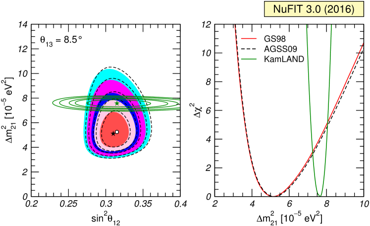
Also for illustration of the independence of these results with respect to the solar modeling, the solar neutrino regions are shown for two latest versions of the Standard Solar Model, namely the GS98 and the AGSS09 models Bergstrom:2016cbh obtained with two different determinations of the solar abundances Vinyoles:2016djt .
3.2 determination in LBL accelerator experiments versus reactors
Figure 6 illustrates the contribution to the present determination of from the different data sets. In the left panels we focus on the determination from long baseline experiments, which is mainly from disappearance data. We plot the and allowed regions (2 dof) in the dominant parameters and . As seen in the figure, although the agreement between the different experiments is reasonable, some “tension” starts to appear in the determination of both parameters among the LBL accelerator experiments. In particular we see that the recent results from NOA, unlike those from T2K, favor a non-maximal value of . It is important to notice that in the context of mixing the relevant oscillation probabilities for the LBL accelerator experiments also depend on (and on the and parameters which are independently well constrained by solar and KamLAND data). To construct the regions plotted in the left panels of Fig. 6, we adopt the procedure currently followed by the LBL accelerator experiments: we marginalize with respect to , taking into account the information from reactor data by adding a Gaussian penalty term to the corresponding . This is not the same as making a combined analysis of LBL and reactor data as we will quantify in Sec. 3.2.1.
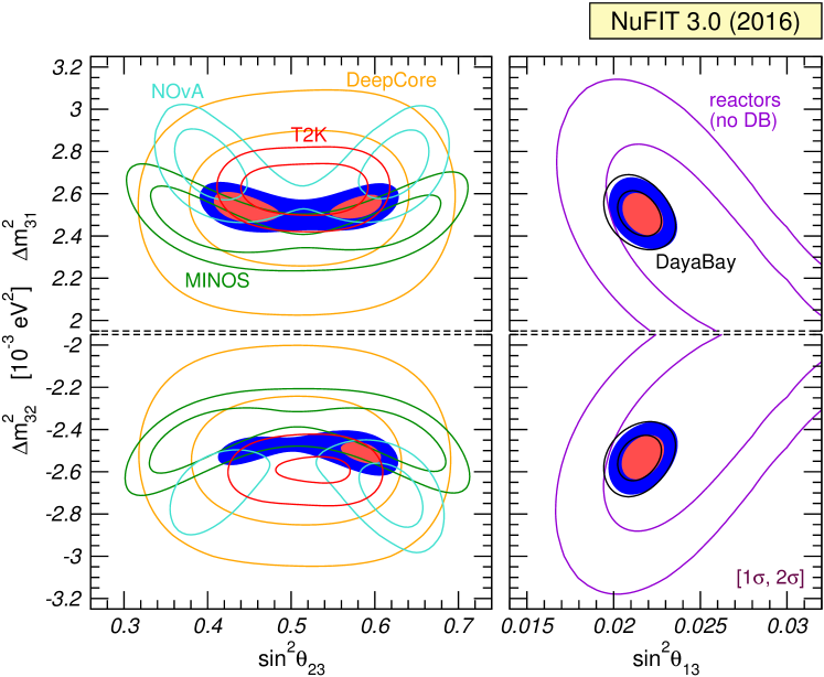
Concerning disappearance data, the total rates observed in reactor experiments at different baselines can provide an independent determination of Bezerra:2012at ; GonzalezGarcia:2012sz . On top of this, the observation of the energy-dependent oscillation effect due to now allows to further strengthen such measurement. In the right panels of Fig. 6 we show therefore the allowed regions in the plane based on global data on disappearance. The violet contours are obtained from all the medium-baselines reactor experiments with the exception of Daya-Bay; these regions emerge from the baseline effect mentioned above plus spectral information from Double-Chooz.333Recently, RENO has presented a spectral analysis based on an exposure of 500 days Seo:2016uom . Here we prefer to include from RENO only the total rate measurement, based on the larger exposure of 800 days reno:nu2014 . The black contours are based on the energy spectrum in Daya-Bay, whereas the colored regions show the combination.
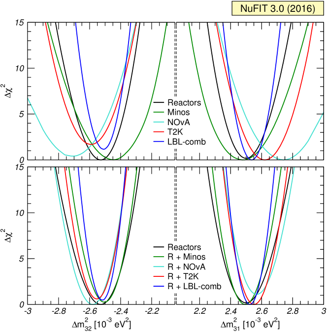
By comparing the left and right panels of Fig. 6 we observe that the combined and disappearance experiments provide a consistent determination of with similar precision. However when comparing the region for each LBL experiment with that of the reactor experiments we find some dispersion in the best fit values and allowed ranges. This is more clearly illustrated in the upper panels of Fig. 7, where we plot the one dimensional projection of the regions in Fig. 6 as a function of after marginalization over for each of the LBL experiments and for their combination, together with that from reactor data after marginalization over . The projections are shown for NO(right) and IO(left). Let us stress that the curves corresponding to LBL experiments in the upper panels of Fig. 7 (as well as those in the upper panels of Figs. 8 and 9) have been obtained by a partial combination of the information on the shown parameter ( or or ) from LBL with that of from reactors, because in these plots only the constraint from reactors is imposed while the dependence on is neglected. This corresponds to the 1-dim projections of the function:
| (5) |
However, since reactor data also depends on the full combination of reactor and LBL results implies that one must add consistently the functions of the LBL experiment with that of reactors evaluated the same value of , this is
| (6) |
We discuss next the effect of combining consistently the information from LBL and reactor experiments in the present determination of , and the ordering.
3.2.1 Impact on the determination of , mass ordering, and
We plot in the lower panels of Figs. 7–9 the one dimensional projections of for each of the parameters , , (marginalized with respect to the two undisplayed parameters) for the consistent LBL+REA combinations with both the information on and from reactors included, Eq. (6). As mentioned before, the curves in the upper panels for these figures show the corresponding 1-dimensional projections for the partial combination, in which only the constraint from reactors is used, Eq. (5). For each experiment the curves in these figures are defined with respect to the global minimum of the two orderings, so the relative height of the minimum in one ordering vs the other gives a measure of the ordering favored by each of the experiments.
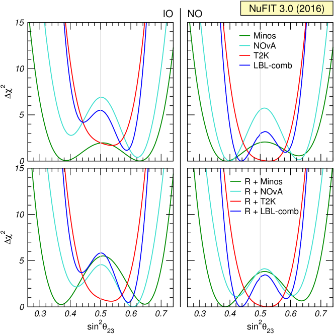
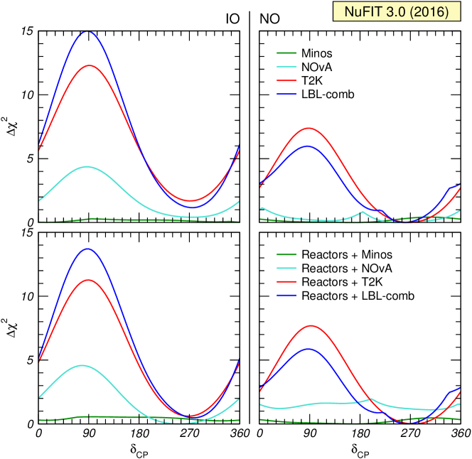
Comparing the upper and lower panels in Figs. 7, 8 and 9 one sees how the contribution to the determination of the mass ordering, the octant and non-maximality of , and the presence of leptonic CP violation of each LBL experiment in the full LBL+REA combination (Eq. 6) can differ from those derived from the LBL results imposing only the constraint from reactors (Eq. 5). This is due to the additional information on from reactors, which is missing in this last case. In particular:
-
•
When only combining the results of the accelerator LBL experiments with the reactor bound of , both NOA and T2K favor NO by () for (T2K). This is in agreement with the analyses shown by the collaborations for example in Refs. nova:nu2016 ; t2k:ichep2016 . However, when consistently combining with the reactor data, we find that the preference for NO by T2K+REA is reduced, and NOA+REA actually favors IO. This is due to the slightly lower value of favored by the reactor data, in particular in comparison with NOA for both orderings, and also with T2K for NO. Altogether we find that for the full combination of LBL accelerator experiments with reactors the “hint” towards NO is below .
-
•
Figure 8 illustrates how both NOA and MINOS favor non-maximal . From this figure we see that while the significance of non-maximality in NOA seems more evident than in MINOS when only the information of is included (upper panels), the opposite holds for the full combination with the reactor data (lower panels). In particular,
(7) for LBL = NOA (MINOS). On the other hand T2K results are compatible with for any ordering. Altogether we find that for NO the full combination of LBL accelerator experiments and reactors disfavor maximal mixing by .
-
•
Regarding the octant of , for IO all LBL accelerator experiments are better described with , adding up to a preference for that octant. Conversely, for NO is favored at .
-
•
From Fig. 9 we see that the “hint” for a CP phase around is mostly driven by T2K data, with some extra contribution from NOA in the case of IO. Within the present precision the favored ranges of in each ordering by the combination of LBL accelerator experiments are pretty independent on the inclusion of the information from reactors.
3.3 Analysis of Super-Kamiokande atmospheric data
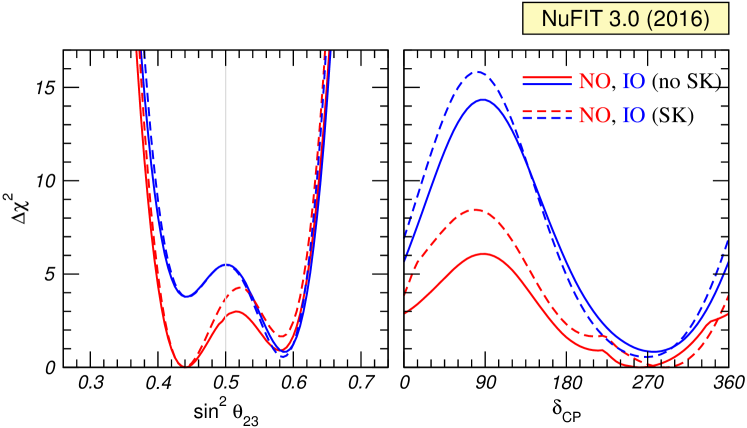
In all the results discussed so far we have not included information from Super-Kamiokande atmospheric data. The reason is that our oscillation analysis cannot reproduce that of the collaboration presented in their talks in the last two years (see for example Ref. skatm:nufact2016 for their latest unpublished results).
| Normal Ordering (best fit) | Inverted Ordering () | Any Ordering | |||
|---|---|---|---|---|---|
| bfp | range | bfp | range | range | |
Already since SK2 the Super-Kamiokande collaboration has been presenting its experimental results in terms of a growing number of data samples. The rates for some of those samples cannot be predicted (and therefore included in a statistical analysis) without a detailed simulation of the detector, which can only be made by the experimental collaboration itself. Our analysis of Super-Kamiokande data has been always based on the “classical” set of samples for which our simulations were reliable enough: sub-GeV and multi-GeV -like and -like fully contained events, as well as partially contained, stopping and through-going muon data, each divided into 10 angular bins for a total of 70 energy and zenith angle bins (details on our simulation of the data samples and the statistical analysis are given in the Appendix of Ref. GonzalezGarcia:2007ib ). Despite the limitations, until recently our results represented the most up-to-date analysis of the atmospheric neutrino data which could be performed outside the collaboration, and we were able to reproduce with reasonable precision the oscillation results of the full analysis presented by SK – both for what concerns the determination of the dominant parameters and , as well as their rather marginal sensitivity to the subdominant appearance effects driven by (and consequently to and the ordering). Thus we confidently included our own implementation of the Super-Kamiokande in our global fit.
However, in the last two years Super-Kamiokande has developed a new analysis method in which a set of neural network based selections are introduced, some of them with the aim of constructing enriched samples which are then further classified into -like and -like subsamples, thus increasing the sensitivity to subleading parameters such as the mass ordering and Wendell:2014dka ; skatm:thesis . The selection criteria are constructed to exploit the expected differences in the number of charged pions and transverse momentum in the interaction of versus . With this new analysis method Super-Kamiokande has been reporting in talks an increasing sensitivity to the ordering and to : for example, the preliminary results of the analysis of SK1–4 (including 2520 days of SK4) skatm:nufact2016 in combination with the reactor constraint of show a preference for NO with a and variation of with the CP phase at the level of .
Unfortunately, with publicly available information this analysis is not reproducible outside the collaboration. Conversely our “traditional” analysis based on their reproducible data samples continues to show only marginal dependence on these effects. This is illustrated in Fig. 10 and Tab. 2 where we show the impact of inclusion of our last re-analysis of SK atmospheric data using the above mentioned 70 bins in energy and zenith angle.444We use the same data and statistical treatment as in our previous global fit NuFIT 2.0 Gonzalez-Garcia:2014bfa as well as in versions 2.1 and 2.2 nufit which is based on 4581 days of data from SK1–4 Wendell:2014dka (corresponding to 1775 days of SK4). We only show the impact on the determination of , , and the mass ordering as the effect on all other parameters is negligible. We observe that for maximal mixing and the second octant receive an additional contribution of about 1 unit in the case of NO, whereas the result for IO is practically unchanged. Values of are slightly more disfavoured, whereas there is basically no effect on the mass ordering discrimination.
In summary, with the information at hand we are not able to reproduce the elements driving the main dependence on the subdominant effects of the official (though preliminary and unpublished) Super-Kamiokande results, while the dominant parameters are currently well determined by LBL experiments. For these reasons we have decided not to include our re-analysis of Super-Kamiokande data in our preferred global fit presented in the previous section. Needless to say that when enough quantitative information becomes available to allow a reliable simulation of the subdominant -driven effects, we will proceed to include it in our global analysis.
4 Monte Carlo evaluation of confidence levels for , and ordering
At present the three least known neutrino oscillation parameters are the Dirac CP violating phase , the octant of and the mass ordering (which in what follows we will denote by “O”). In order to study the information from data on these parameters one can use two test statistics Elevant:2015ska ; Blennow:2014sja :
| (8) | ||||
| (9) |
where the minimization in the first equation is performed with respect to all oscillation parameters except and the ordering (), while in the second equation the minimization is over all oscillation parameters except and the ordering (). Here indicates the minimum with respect to all oscillation parameters including the mass ordering.
We have plotted the values of these test statistics in the lower right and central left panels in Fig. 2. We can use them not only for the determination of and , respectively, but also of the mass ordering. For instance, using Eq. (8) we can determine a confidence interval for at a given CL for both orderings. However, below a certain CL no interval will appear for the less favored ordering. In this sense we can exclude that ordering at the CL at which the corresponding interval for disappears. Note that a similar prescription to test the mass ordering can be built for any other parameter as well, e.g., for using Eq. (9).555Let us mention that this method to determine the mass ordering is different from the one based on the test statistics discussed in Ref. Blennow:2013oma .
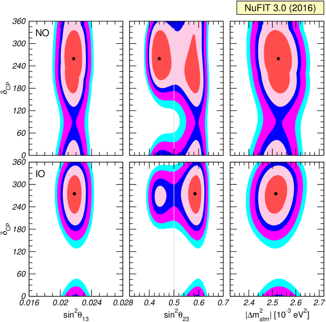
In Sec. 2 we have presented confidence intervals assuming that the test statistics follow a -distribution with 1 dof, relying on Wilks theorem to hold Wilks:1938dza (this is what we call the Gaussian limit). However, the test statistics in Eqs. (8) and (9) are expected not to follow Wilks’ theorem because of several reasons Elevant:2015ska :
-
•
Sensitivity of current data to is still limited, as can be seen in Fig. 2: all values of have , and for NO not even is attained.
-
•
Regarding , its precision is dominated by disappearance experiments. Since the relevant survival probability depends dominantly on , there is both a physical boundary of their parameter space at (because ), as well as a degeneracy related to the octant.
-
•
The mass ordering is a discrete parameter.
-
•
The dependence of the theoretical predictions on is significantly non-linear, even more considering the periodic nature of this parameter. Furthermore, there are complicated correlations and degeneracies between , , and the mass ordering (see Fig. 11 for illustration).
Therefore, one may expect deviations from the Gaussian limit of the distributions, and confidence levels for these parameters should be cross checked through a Monte Carlo simulation of the relevant experiments. We consider in the following the combination of the T2K, NOA, MINOS and Daya-Bay experiments, which are most relevant for the parameters we are interested in this section. For a given point of assumed true values for the parameters we generate a large number () of pseudo-data samples for each of the experiments. For each pseudo-data sample we compute the two statistics given in Eqs. (8) and (9) to determine their distributions numerically. In Ref. Elevant:2015ska it has been shown that the distribution of test statistics for 2-dimensional parameter region (such as for instance the middle panels of Fig. 11) are more close to Gaussianity than 1-dimensional ones such as Eqs. (8) and (9). Therefore we focus here on the 1-dimensional cases.
First, let us note that in order to keep calculation time manageable one can fix all parameters which are known to be uncorrelated with the three we are interested in (i.e., , , O). This is certainly the case for and which are determined independently by solar and KamLAND data. As for , presently the most precise information arises from reactor data whose results are insensitive to and . Consequently, marginalizing over within reactor uncertainties or fixing it to the best fit value gives a negligible difference in the simulations. Concerning we observe that there are no strong correlations or degeneracies with (see Fig. 11), and we assume that the distributions of the test statistics do not significantly depend on the assumed true value. Therefore we consider only the global best fit values for each ordering as true values for to generate pseudo-data. However, since the relevant observables do depend non-trivially on its value, it is important to keep as a free parameter in the fit and to minimize the for each pseudo-data sample with respect to it. Hence, we approximate the test statistics in Eqs. (8) and (9) by using
| (10) | ||||
| (11) |
with the other oscillation parameters kept fixed at their best fit points: , , and .
4.1 and the mass ordering
The value of the test statistics (8) is shown in Fig. 12 for the combination of T2K, NOA, MINOS and Daya-Bay as a function of for both mass orderings. In the generation of the pseudo-data we have assumed three representative values of as shown in the plots. The broken curves show, for each set of true values, the values of which are larger than 68%, 95%, and 99% of all generated data samples.
From the figure we read that if the from real data (solid curve, identical in the three panels) for a given ordering is above the CL lines for that ordering for a given value of , that value of and the mass ordering can be rejected with confidence. So if the minimum of the curve for one of the orderings (in this case IO is the one with non-zero minimum) is above the CL line one infers that that ordering is rejected at that CL.
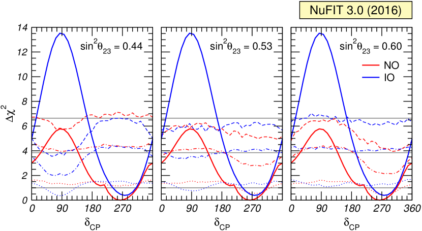
For the sake of comparison we also show in Fig. 12 the corresponding 68%, 95% and 99% Gaussian confidence levels as horizontal lines. There are some qualitative deviations from Gaussianity that have already been reported Elevant:2015ska :
-
•
For , , and IO as well as for , and NO, the confidence levels decrease. This effect arises because at those points in parameter space the oscillation probability has a minimum or a maximum, respectively. Therefore, statistical fluctuations leading to less (or more) events than predicted cannot be accommodated by adjusting the parameters. is small more often and the confidence levels decrease. This is an effect always present at boundaries in parameter space, usually referred to as an effective decrease in the number of degrees of freedom in the model.
-
•
Conversely for for , and for , the confidence levels increase. This is associated with the prominent presence of the octant degeneracy. Degeneracies imply that statistical fluctuations can drive you away from the true value, increases, and the confidence levels increase. This is usually referred to as an effective increase in the number of degrees of freedom in the model due to degeneracies.
-
•
Overall we find that with present data confidence levels are clearly closer to Gaussianity than found in Refs. Gonzalez-Garcia:2014bfa ; Elevant:2015ska , where similar simulations have been performed with less data available. For those data sets confidence levels were consistently below their Gaussian limit. This was mainly a consequence of the limited statistics and the cyclic nature of which lead to an effective decrease in the number of degrees of freedom. We now find that when the full combination of data currently available is included this effect is reduced, as expected if experiments become more sensitive.
-
•
For all true values considered, IO is not rejected even at . In particular we find IO disfavored at for .
| Ordering | CP cons. | 90% CL range | 95% CL range | |
| 0.44 | NO | 70% | ||
| IO | 98% | |||
| 0.53 | NO | 70% | ||
| IO | 98% | |||
| 0.60 | NO | 70% | ||
| IO | 97% | |||
| Gaussian | NO | 80% | ||
| IO | 97% |
Quantitatively we show in Tab. 3 the CL at which CP conservation () is disfavored as well as the 90% and 95% confidence intervals for . We find that the CL of rejection of CP conservation as well as the allowed ranges do not depend very significantly on . This can be understood from Fig. 12: the dependence on occur mostly for and IO, a region discarded with a large CL, and for and NO, a region around the best fit.
Note that in the table the intervals for are defined for both orderings with respect to the global minimum (which happens for NO). Hence the intervals for IO include the effect that IO is slightly disfavored with respect to NO. They cannot be directly compared to the intervals given in Tab. 1, where we defined intervals relative to the local best fit point for each ordering.
A similar comment applies also to the CL quoted in the table to reject CP conservation. For IO this is defined relative to the best fit point in NO. We find that for NO, CP conservation is allowed at 70% CL, i.e., slightly above (with some deviations from the Gaussian result of 80% CL), while for IO the CL for CP conservation is above . Note that values of are disfavored at around 99% CL for NO, while for IO the rejection is at even higher CL: the with respect to the global minimum is around 14, which would correspond to in the Gaussian limit. Our Monte Carlo sample of pseudo-data sets is not large enough to confirm such a high confidence level.
4.2 and the mass ordering
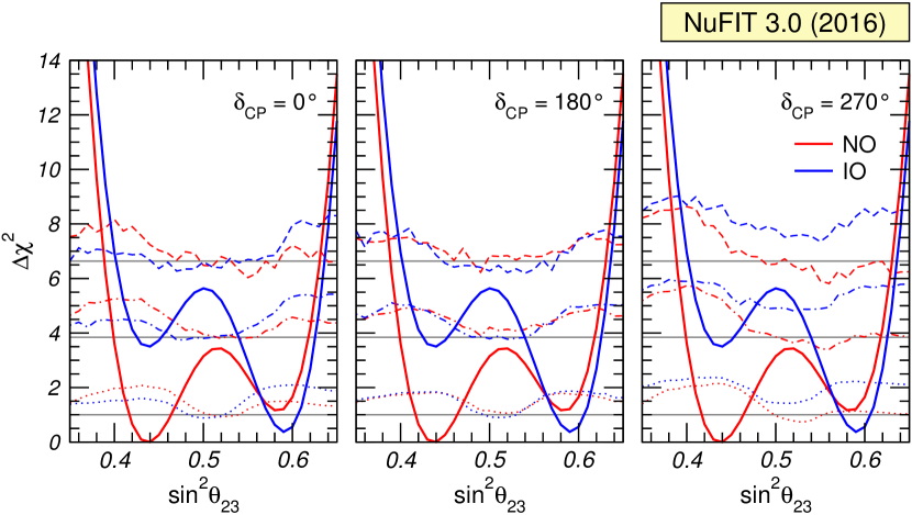
Moving now to the discussion of , we show the value of the test statistics (9) in Fig. 13 for the combination of T2K, NOA, MINOS and Daya-Bay experiments as a function of , for both mass orderings. For the generation of the pseudo-data we have assumed three example values . We do not show results for , since this value is already quite disfavored by data, especially for IO.666We are aware of the fact that this choice is somewhat arbitrary and implicitly resembles Bayesian reasoning. In the strict frequentist sense we cannot a priori exclude any true value of the parameters. The broken curves show for each set of true values, the values of which are larger than 68%, 95%, and 99% of all generated data samples. From the figure we see that the deviations from Gaussianity are not very prominent and can be understood as follows:
-
•
The confidence levels decrease around maximal mixing because of the boundary on the parameter space present at maximal mixing for disappearance data.
-
•
There is some increase and decrease in the confidence levels for , in the same parameter region as the corresponding ones in Fig. 12.
| Ordering | 90% CL range | 95% CL range | ||
| NO | 92% | |||
| IO | 98% | |||
| NO | 91% | |||
| IO | 98% | |||
| NO | 92% | |||
| IO | 97% | |||
| Gaussian | NO | 92% | ||
| IO | 98% |
In Tab. 4 we show the CL at which the combination of LBL and reactor experiments can disfavor maximal mixing () as well as the 90% and 95% confidence intervals for for both orderings with respect to the global best fit. We observe from the table that the Gaussian approximation is quite good for both, the CL of maximal mixing as well as for the confidence intervals. We conclude that present data excludes maximal mixing at slightly more than 90% CL. Again we note that the intervals for for IO cannot be directly compared with the ones from Tab. 1, where they are defined with respect to the local minimum in each ordering.
| NO/2nd Oct. | IO/1st Oct. | IO/2nd Oct. | |
|---|---|---|---|
| 62% | 91% | 28% | |
| 56% | 89% | 32% | |
| 70% | 83% | 27% | |
| Gaussian | 72% | 94% | 46% |
In Tab. 5 we show the CL at which a certain combination of mass ordering and octant can be excluded with respect to the global minimum in the NO and 1st octant. We observe that the CL of the second octant for NO shows relatively large deviations from Gaussianity and dependence on the true value of . In any case, the sensitivity is very low and the 2nd octant can be reject at most at 70% CL () for all values of . The first octant for IO can be excluded at between 83% and 91% CL, depending on . As discussed above, the exclusion of the IO/2nd octant case corresponds also to the exclusion of the IO, since at that point the confidence interval in IO would vanish. Also in this case we observe deviations from the Gaussian approximation and the CL of at best 32% is clearly less than (consistent with the results discussed in the previous subsection), showing that the considered data set has essentially no sensitivity to the mass ordering.
5 Conclusions
We have presented the results of the updated (as of fall 2016) analysis of relevant neutrino data in the framework of mixing among three massive neutrinos. Quantitatively the present determination of the two mass differences, three mixing angles and the relevant CP violating phase obtained under the assumption that their log-likelihood follows a distribution is listed in Table 1, and the corresponding leptonic mixing matrix is given in Eq. (2). We have found that the maximum allowed CP violation in the leptonic sector parametrized by the Jarlskog determinant is at ().
We have studied in detail how the sensitivity to the least-determined parameters , and the mass ordering depends on the proper combination of the different data samples (Sec. 3.2). Furthermore we have quantified deviations from the Gaussian approximation in the evaluation of the confidence intervals for and by performing a Monte Carlo study of the long baseline accelerator and reactor results (Sec. 4). We can summarize the main conclusions in these sections as follows:
-
•
At present the precision on the determination of from disappearance in LBL accelerator experiments NOA, T2K and MINOS is comparable to that from disappearance in reactor experiments, in particular with the spectral information from Daya-Bay. When comparing the region for each LBL experiment with that of the reactor experiments we find some dispersion in the best fit values and allowed ranges.
-
•
The interpretation of the data from accelerator LBL experiments in the framework of mixing requires using information from the reactor experiments, in particular about the mixing angle . But since, as mentioned above, reactor data also constrain , the resulting CL of presently low confidence effects (in particular the non-maximality of and the mass ordering) is affected by the inclusion of this information in the combination.
-
•
We find that the mass ordering favored by NOA changes from NO to IO when the information on from reactor experiments is correctly included in the LBL+REA combination, and the of NO in T2K is reduced from around 2 to 0.5 (see Fig. 7). Our MC study of the combination of LBL and reactor data shows that for all cases generated, NO is favored but with a CL of less than .
-
•
About the non-maximality of , we find that when the information on from reactor experiments is correctly included in the LBL+REA combination, it is not NOA but actually MINOS which contributes most to the preference for non-maximal (see Fig. 8). Quantitatively our MC study of the combination of LBL and reactor data shows that for all the cases generated the CL for rejection of maximal is about 92% for NO. As seen in Fig. 13 and Tab. 4, the CL of maximal mixing as well as confidence intervals for derived with MC simulations are not very different from the corresponding Gaussian approximation.
-
•
The same study shows that for NO (IO) the favored octant is (). The CL for rejection of the disfavored octant depends on the true value of assumed in the MC study and it is generically lower than the one obtained in the Gaussian limit (see Tab. 5). For example, for NO the second octant is disfavored at a confidence level between and depending on the assumed true value of .
-
•
The present sensitivity to is driven by T2K with a minor contribution from NOA for IO (see Fig. 9). The dependence of the combined CL of the “hint” towards leptonic CP violation and in particular for on the true value of is shown in Fig. 12, from which we read that for all cases generated CP conservation is disfavored only at 70% () for NO. Values of are disfavored at around 99% CL for NO, while for IO the rejection is at higher CL ( with respect to the global minimum).
Finally we comment that the increased statistics in SK4 and Borexino has had no major impact in the long-standing tension between the best fit values of as determined from the analysis of KamLAND and solar data, which remains an unresolved effect.
Future updates of this analysis will be provided at the NuFIT website quoted in Ref. nufit .
Acknowledgments
This work is supported by USA-NSF grant PHY-1620628, by EU Networks FP10 ITN ELUSIVES (H2020-MSCA-ITN-2015-674896) and INVISIBLES-PLUS (H2020-MSCA-RISE-2015-690575), by MINECO grants FPA2013-46570, FPA2012-31880 and MINECO/FEDER-UE grant FPA2015-65929-P, by Maria de Maetzu program grant MDM-2014-0367 of ICCUB, and the “Severo Ochoa” program grant SEV-2012-0249 of IFT. I.E. acknowledges support from the FPU program fellowship FPU15/03697.
Appendix A List of data used in the analysis
Solar experiments
-
•
Chlorine total rate Cleveland:1998nv , 1 data point.
-
•
Gallex & GNO total rates Kaether:2010ag , 2 data points.
-
•
SAGE total rate Abdurashitov:2009tn , 1 data point.
-
•
SK1 full energy and zenith spectrum Hosaka:2005um , 44 data points.
-
•
SK2 full energy and day/night spectrum Cravens:2008aa , 33 data points.
-
•
SK3 full energy and day/night spectrum Abe:2010hy , 42 data points.
-
•
SK4 2055-day day-night asymmetry sksol:nakano2016 and 2365-day energy spectrum sksol:ichep2016 , 24 data points.
-
•
SNO combined analysis Aharmim:2011vm , 7 data points.
-
•
Borexino Phase-I 740.7-day low-energy data Bellini:2011rx , 33 data points.
-
•
Borexino Phase-I 246-day high-energy data Bellini:2008mr , 6 data points.
-
•
Borexino Phase-II 408-day low-energy data Bellini:2014uqa , 42 data points.
Atmospheric experiments
-
•
IceCube/DeepCore 3-year data Aartsen:2014yll ; deepcore:2016 , 64 data points.
Reactor experiments
-
•
KamLAND combined DS1 & DS2 spectrum Gando:2010aa , 17 data points.
-
•
CHOOZ energy spectrum Apollonio:1999ae , 14 data points.
-
•
Palo-Verde total rate Piepke:2002ju , 1 data point.
-
•
Double-Chooz FD-I (461 days) and FD-II (212 days) spectra dc:moriond2016 , 54 data points.
-
•
Daya-Bay 1230-day spectrum db:nu2016 , 34 data points.
-
•
Reno 800-day near & far total rates reno:nu2014 , 2 data points (with free normalization).
-
•
SBL reactor data (including Daya-Bay total flux at near detector), 77 data points Kopp:2013vaa ; db:nu2014 .
Accelerator experiments
-
•
MINOS pot -disappearance data Adamson:2013whj , 39 data points.
-
•
MINOS pot -disappearance data Adamson:2013whj , 14 data points.
-
•
MINOS pot -appearance data Adamson:2013ue , 5 data points.
-
•
MINOS pot -appearance data Adamson:2013ue , 5 data points.
-
•
T2K pot -disappearance data t2k:ichep2016 ; t2k:susy2016 , 28 data points.
-
•
T2K pot -appearance data t2k:ichep2016 ; t2k:susy2016 , 5 data points.
-
•
T2K pot -disappearance data t2k:ichep2016 ; t2k:susy2016 , 63 data points.
-
•
T2K pot -appearance data t2k:ichep2016 ; t2k:susy2016 , 1 data point.
-
•
NOA pot -disappearance data nova:nu2016 , 18 data points.
-
•
NOA pot -appearance data nova:nu2016 , 10 data points.
References
- (1) B. Pontecorvo, Neutrino experiments and the question of leptonic-charge conservation, Sov. Phys. JETP 26 (1968) 984–988.
- (2) V. N. Gribov and B. Pontecorvo, Neutrino astronomy and lepton charge, Phys. Lett. B28 (1969) 493.
- (3) M. C. Gonzalez-Garcia and M. Maltoni, Phenomenology with Massive Neutrinos, Phys. Rept. 460 (2008) 1–129, [0704.1800].
- (4) C. Giunti, Light Sterile Neutrinos: Status and Perspectives, Nucl. Phys. B908 (2016) 336–353, [1512.04758].
- (5) Z. Maki, M. Nakagawa and S. Sakata, Remarks on the unified model of elementary particles, Prog. Theor. Phys. 28 (1962) 870–880.
- (6) M. Kobayashi and T. Maskawa, CP Violation in the Renormalizable Theory of Weak Interaction, Prog. Theor. Phys. 49 (1973) 652–657.
- (7) S. M. Bilenky, J. Hosek and S. T. Petcov, On Oscillations of Neutrinos with Dirac and Majorana Masses, Phys. Lett. B94 (1980) 495.
- (8) P. Langacker, S. T. Petcov, G. Steigman and S. Toshev, On the Mikheev-Smirnov-Wolfenstein (MSW) Mechanism of Amplification of Neutrino Oscillations in Matter, Nucl. Phys. B282 (1987) 589.
- (9) M. C. Gonzalez-Garcia, M. Maltoni and T. Schwetz, Updated fit to three neutrino mixing: status of leptonic CP violation, JHEP 11 (2014) 052, [1409.5439].
- (10) F. Capozzi, E. Lisi, A. Marrone, D. Montanino and A. Palazzo, Neutrino masses and mixings: Status of known and unknown parameters, Nucl. Phys. B908 (2016) 218–234, [1601.07777].
- (11) D. V. Forero, M. Tortola and J. W. F. Valle, Neutrino oscillations refitted, Phys. Rev. D90 (2014) 093006, [1405.7540].
- (12) H. Minakata, H. Sugiyama, O. Yasuda, K. Inoue and F. Suekane, Reactor measurement of theta(13) and its complementarity to long baseline experiments, Phys. Rev. D68 (2003) 033017, [hep-ph/0211111]. [Erratum: Phys. Rev.D70,059901(2004)].
- (13) P. Huber, M. Lindner, T. Schwetz and W. Winter, Reactor neutrino experiments compared to superbeams, Nucl. Phys. B665 (2003) 487–519, [hep-ph/0303232].
- (14) P. Huber, M. Lindner, M. Rolinec, T. Schwetz and W. Winter, Prospects of accelerator and reactor neutrino oscillation experiments for the coming ten years, Phys. Rev. D70 (2004) 073014, [hep-ph/0403068].
- (15) B. T. Cleveland et al., Measurement of the solar electron neutrino flux with the Homestake chlorine detector, Astrophys. J. 496 (1998) 505–526.
- (16) F. Kaether, W. Hampel, G. Heusser, J. Kiko and T. Kirsten, Reanalysis of the GALLEX solar neutrino flux and source experiments, Phys. Lett. B685 (2010) 47–54, [1001.2731].
- (17) SAGE collaboration, J. N. Abdurashitov et al., Measurement of the solar neutrino capture rate with gallium metal. III: Results for the 2002–2007 data-taking period, Phys. Rev. C80 (2009) 015807, [0901.2200].
- (18) Super-Kamiokande collaboration, J. Hosaka et al., Solar neutrino measurements in Super-Kamiokande-I, Phys. Rev. D73 (2006) 112001, [hep-ex/0508053].
- (19) Super-Kamiokande collaboration, J. Cravens et al., Solar neutrino measurements in Super-Kamiokande-II, Phys. Rev. D78 (2008) 032002, [0803.4312].
- (20) Super-Kamiokande collaboration, K. Abe et al., Solar neutrino results in Super-Kamiokande-III, Phys. Rev. D83 (2011) 052010, [1010.0118].
- (21) Y. Nakano, 8B solar neutrino spectrum measurement using Super-Kamiokande IV. PhD thesis, Tokyo U., 2016-02.
- (22) Y. Nakano, “Solar neutrino results from Super-Kamiokande.” Talk given at the 38th International Conference on High Energy Physics, Chicago, USA, August 3–10, 2016.
- (23) SNO collaboration, B. Aharmim et al., Combined Analysis of all Three Phases of Solar Neutrino Data from the Sudbury Neutrino Observatory, Phys. Rev. C88 (2013) 025501, [1109.0763].
- (24) Borexino collaboration, G. Bellini et al., Precision measurement of the 7Be solar neutrino interaction rate in Borexino, Phys. Rev. Lett. 107 (2011) 141302, [1104.1816].
- (25) Borexino collaboration, G. Bellini et al., Measurement of the solar 8B neutrino rate with a liquid scintillator target and 3 MeV energy threshold in the Borexino detector, Phys. Rev. D82 (2010) 033006, [0808.2868].
- (26) BOREXINO collaboration, G. Bellini et al., Neutrinos from the primary proton–proton fusion process in the Sun, Nature 512 (2014) 383–386.
- (27) MINOS collaboration, P. Adamson et al., Measurement of Neutrino and Antineutrino Oscillations Using Beam and Atmospheric Data in MINOS, Phys. Rev. Lett. 110 (2013) 251801, [1304.6335].
- (28) MINOS collaboration, P. Adamson et al., Electron neutrino and antineutrino appearance in the full MINOS data sample, Phys. Rev. Lett. (2013) , [1301.4581].
- (29) K. Iwamoto, “Recent Results from T2K and Future Prospects.” Talk given at the 38th International Conference on High Energy Physics, Chicago, USA, August 3–10, 2016.
- (30) A. Cervera, “Latest Results from Neutrino Oscillation Experiments.” Talk given at the SUSY 2016 Conference, Melbourne, Australia, July 3–8, 2016.
- (31) P. Vahle, “New results from NOvA.” Talk given at the XXVII International Conference on Neutrino Physics and Astrophysics, London, UK, July 4–9, 2016.
- (32) KamLAND collaboration, A. Gando et al., Constraints on from A Three-Flavor Oscillation Analysis of Reactor Antineutrinos at KamLAND, Phys. Rev. D83 (2011) 052002, [1009.4771].
- (33) CHOOZ collaboration, M. Apollonio et al., Limits on Neutrino Oscillations from the CHOOZ Experiment, Phys. Lett. B466 (1999) 415–430, [hep-ex/9907037].
- (34) Palo Verde collaboration, A. Piepke, Final results from the Palo Verde neutrino oscillation experiment, Prog. Part. Nucl. Phys. 48 (2002) 113–121.
- (35) M. Ishitsuka, “New results of Double Chooz.” Talk given at the Conference Rencontres de Moriond EW 2016, La Thuile, Italy, March 12–19, 2016.
- (36) Z. Yu, “Recent Results from the Daya Bay Experiment.” Talk given at the XXVII International Conference on Neutrino Physics and Astrophysics, London, UK, July 4–9, 2016.
- (37) S.-H. Seo, “New Results from RENO.” Talk given at the XXVI International Conference on Neutrino Physics and Astrophysics, Boston, USA, June 2–7, 2014.
- (38) J. Kopp, P. A. N. Machado, M. Maltoni and T. Schwetz, Sterile Neutrino Oscillations: The Global Picture, JHEP 1305 (2013) 050, [1303.3011].
- (39) H. Kwon, F. Boehm, A. Hahn, H. Henrikson, J. Vuilleumier et al., Search for neutrino oscillations at a fission reactor, Phys.Rev. D24 (1981) 1097–1111.
- (40) CALTECH-SIN-TUM collaboration, G. Zacek et al., Neutrino Oscillation Experiments at the Gosgen Nuclear Power Reactor, Phys.Rev. D34 (1986) 2621–2636.
- (41) G. Vidyakin, V. Vyrodov, I. Gurevich, Y. Kozlov, V. Martemyanov et al., Detection of anti-neutrinos in the flux from two reactors, Sov.Phys.JETP 66 (1987) 243–247.
- (42) G. Vidyakin, V. Vyrodov, Y. Kozlov, A. Martemyanov, V. Martemyanov et al., Limitations on the characteristics of neutrino oscillations, JETP Lett. 59 (1994) 390–393.
- (43) A. Afonin, S. Ketov, V. Kopeikin, L. Mikaelyan, M. Skorokhvatov et al., A study of the reaction on a nuclear reactor, Sov.Phys.JETP 67 (1988) 213–221.
- (44) A. Kuvshinnikov, L. Mikaelyan, S. Nikolaev, M. Skorokhvatov and A. Etenko, Measuring the cross-section and beta decay axial constant in a new experiment at Rovno NPP reactor. (In Russian), JETP Lett. 54 (1991) 253–257.
- (45) Y. Declais, J. Favier, A. Metref, H. Pessard, B. Achkar et al., Search for neutrino oscillations at 15-meters, 40-meters, and 95-meters from a nuclear power reactor at Bugey, Nucl.Phys. B434 (1995) 503–534.
- (46) Y. Declais, H. de Kerret, B. Lefievre, M. Obolensky, A. Etenko et al., Study of reactor anti-neutrino interaction with proton at Bugey nuclear power plant, Phys.Lett. B338 (1994) 383–389.
- (47) Z. D. Greenwood et al., Results of a two position reactor neutrino oscillation experiment, Phys. Rev. D53 (1996) 6054–6064.
- (48) IceCube collaboration, M. Aartsen et al., Determining neutrino oscillation parameters from atmospheric muon neutrino disappearance with three years of IceCube DeepCore data, Phys. Rev. D91 (2015) 072004, [1410.7227].
- (49) NuFIT webpage, http://www.nu-fit.org.
- (50) M. Gonzalez-Garcia, M. Maltoni, J. Salvado and T. Schwetz, Global fit to three neutrino mixing: critical look at present precision, JHEP 1212 (2012) 123, [1209.3023].
- (51) T. Mueller, D. Lhuillier, M. Fallot, A. Letourneau, S. Cormon et al., Improved Predictions of Reactor Antineutrino Spectra, Phys.Rev. C83 (2011) 054615, [1101.2663].
- (52) P. Huber, On the determination of anti-neutrino spectra from nuclear reactors, Phys.Rev. C84 (2011) 024617, [1106.0687].
- (53) G. Mention, M. Fechner, T. Lasserre, T. Mueller, D. Lhuillier et al., The Reactor Antineutrino Anomaly, Phys.Rev. D83 (2011) 073006, [1101.2755].
- (54) T. Schwetz, What is the probability that theta(13) and CP violation will be discovered in future neutrino oscillation experiments?, Phys. Lett. B648 (2007) 54--59, [hep-ph/0612223].
- (55) M. Blennow, P. Coloma and E. Fernandez-Martinez, Reassessing the sensitivity to leptonic CP violation, JHEP 03 (2015) 005, [1407.3274].
- (56) M. C. Gonzalez-Garcia and C. Pena-Garay, Three neutrino mixing after the first results from K2K and KamLAND, Phys. Rev. D68 (2003) 093003, [hep-ph/0306001].
- (57) C. Jarlskog, Commutator of the Quark Mass Matrices in the Standard Electroweak Model and a Measure of Maximal CP Violation, Phys.Rev.Lett. 55 (1985) 1039.
- (58) K. A. Olive, Review of Particle Physics, Chin. Phys. C40 (2016) 100001.
- (59) L. Wolfenstein, Neutrino oscillations in matter, Phys. Rev. D17 (1978) 2369--2374.
- (60) S. P. Mikheev and A. Y. Smirnov, Resonance enhancement of oscillations in matter and solar neutrino spectroscopy, Sov. J. Nucl. Phys. 42 (1985) 913--917.
- (61) J. Bergstrom, M. C. Gonzalez-Garcia, M. Maltoni, C. Pena-Garay, A. M. Serenelli and N. Song, Updated determination of the solar neutrino fluxes from solar neutrino data, JHEP 03 (2016) 132, [1601.00972].
- (62) N. Vinyoles, A. M. Serenelli, F. L. Villante, S. Basu, J. Bergström, M. C. Gonzalez-Garcia et al., A new Generation of Standard Solar Models, 1611.09867.
- (63) T. J. C. Bezerra, H. Furuta and F. Suekane, Measurement of Effective using Baseline Differences of Daya Bay, RENO and Double Chooz Reactor Neutrino Experiments, 1206.6017.
- (64) H. Seo et al., Spectral Measurement of the Electron Antineutrino Oscillation Amplitude and Frequency using 500 Live Days of RENO Data, 1610.04326.
- (65) Super-Kamiokande collaboration, R. Wendell, Atmospheric Results from Super-Kamiokande, AIP Conf. Proc. 1666 (2015) 100001, [1412.5234].
- (66) J. Kameda, ‘‘Recent results from Super-Kamokande on atmospheric neutrinos and next project: Hyper-Kamioande.’’ Talk given at the XII Rencontres de Vietnam: NuFact 2016, Qui Nhon, Vietnam, August 21--27, 2016.
- (67) K. P. Lee, ‘‘Study of the neutrino mass hierarchy with the atmospheric neutrino data observed in SuperKamiokande.’’ Ph.D. thesis, The University of Tokyo, 2012.
- (68) J. Elevant and T. Schwetz, On the determination of the leptonic CP phase, JHEP 09 (2015) 016, [1506.07685].
- (69) M. Blennow, P. Coloma, P. Huber and T. Schwetz, Quantifying the sensitivity of oscillation experiments to the neutrino mass ordering, JHEP 03 (2014) 028, [1311.1822].
- (70) S. S. Wilks, The Large-Sample Distribution of the Likelihood Ratio for Testing Composite Hypotheses, Annals Math. Statist. 9 (1938) 60--62.
- (71) IceCube collaboration, J. P. Yañez et al., ‘‘IceCube Oscillations: 3 years muon neutrino disappearance data.’’ http://icecube.wisc.edu/science/data/nu_osc.
- (72) C. Zhang, ‘‘Recent Results From Daya Bay.’’ Talk given at the XXVI International Conference on Neutrino Physics and Astrophysics, Boston, USA, June 2--7, 2014.