Deep Information Propagation

Samuel S. Schoenholz
Google Brain &Justin Gilmer
Google Brain &Surya Ganguli
Stanford University &Jascha Sohl-Dickstein
Google Brain
Work done as a member of the Google Brain Residency program (g.co/brainresidency)
Abstract

We study the behavior of untrained neural networks whose weights and biases are randomly distributed using mean field theory. We show the existence of depth scales that naturally limit the maximum depth of signal propagation through these random networks. Our main practical result is to show that random networks may be trained precisely when information can travel through them. Thus, the depth scales that we identify provide bounds on how deep a network may be trained for a specific choice of hyperparameters. As a corollary to this, we argue that in networks at the edge of chaos, one of these depth scales diverges. Thus arbitrarily deep networks may be trained only sufficiently close to criticality. We show that the presence of dropout destroys the order-to-chaos critical point and therefore strongly limits the maximum trainable depth for random networks. Finally, we develop a mean field theory for backpropagation and we show that the ordered and chaotic phases correspond to regions of vanishing and exploding gradient respectively.

1 Introduction

Deep neural network architectures have become ubiquitous in machine learning. The success of deep networks is due to the fact that they are highly expressive (Montufar et al., 2014) while simultaneously being relatively easy to optimize (Choromanska et al., 2015; Goodfellow et al., 2014) with strong generalization properties (Recht et al., 2015). Consequently, developments in machine learning often accompany improvements in our ability to train increasingly deep networks. Despite this, designing novel network architectures is frequently equal parts art and science. This is, in part, because a general theory for neural networks that might inform design decisions has lagged behind the feverish pace of design.

A pair of recent papers (Poole et al., 2016; Raghu et al., 2016) demonstrated that random neural networks are exponentially expressive in their depth. Central to their approach was the consideration of networks after random initialization, whose weights and biases were i.i.d. Gaussian distributed. In particular the paper by Poole et al. (2016) developed a “mean field” formalism for treating wide, untrained, neural networks. They showed that these mean field networks exhibit an order-to-chaos transition as a function of the weight and bias variances. Notably the mean field formalism is not closely tied to a specific choice of activation function or loss.

In this paper, we demonstrate the existence of several characteristic “depth” scales that emerge naturally and control signal propagation in these random networks. We then show that one of these depth scales, ξcsubscript𝜉𝑐\xi_{c}, diverges at the boundary between order and chaos. This result is insensitive to many architectural decisions (such as choice of activation function) and will generically be true at any order-to-chaos transition. We then extend these results to include dropout and we show that even small amounts of dropout destroys the order-to-chaos critical point and consequently removes the divergence in ξcsubscript𝜉𝑐\xi_{c}. Together these results bound the depth to which signal may propagate through random neural networks.

We then develop a corresponding mean field model for gradients and we show that a duality exists between the forward propagation of signals and the backpropagation of gradients. The ordered and chaotic phases that Poole et al. (2016) identified correspond to regions of vanishing and exploding gradients, respectively. We demonstrate the validity of this mean field theory by computing gradients of random networks on MNIST. This provides a formal explanation of the ‘vanishing gradients’ phenomenon that has long been observed in neural networks (Bengio et al., 1993). We continue to show that the covariance between two gradients is controlled by the same depth scale that limits correlated signal propagation in the forward direction.

Finally, we hypothesize that a necessary condition for a random neural network to be trainable is that information should be able to pass through it. Thus, the depth-scales identified here bound the set of hyperparameters that will lead to successful training. To test this ansatz we train ensembles of deep, fully connected, feed-forward neural networks of varying depth on MNIST and CIFAR10, with and without dropout. Our results confirm that neural networks are trainable precisely when their depth is not much larger than ξcsubscript𝜉𝑐\xi_{c}. This result is dataset independent and is, therefore, a universal function of network architecture.

A corollary of these result is that asymptotically deep neural networks should be trainable provided they are initialized sufficiently close to the order-to-chaos transition. The notion of “edge of chaos” initialization has been explored previously. Such investigations have been both direct as in Bertschinger et al. (2005); Glorot & Bengio (2010) or indirect, through initialization schemes that favor deep signal propagation such as batch normalization (Ioffe & Szegedy, 2015), orthogonal matrix initialization (Saxe et al., 2014), random walk initialization (Sussillo & Abbott, 2014), composition kernels (Daniely et al., 2016), or residual network architectures (He et al., 2015). The novelty of the work presented here is two-fold. First, our framework predicts the depth at which networks may be trained even far from the order-to-chaos transition. While a skeptic might ask when it would be profitable to initialize a network far from criticality, we respond by noting that there are architectures (such as neural networks with dropout) where no critical point exists and so this more general framework is needed. Second, our work provides a formal, as opposed to intuitive, explanation for why very deep networks can only be trained near the edge of chaos.

2 Background

We begin by recapitulating the mean-field formalism developed in Poole et al. (2016). Consider a fully-connected, untrained, feed-forward, neural network of depth L𝐿L with layer width Nlsubscript𝑁𝑙N_{l} and some nonlinearity ϕ::italic-ϕ\phi:\mathbb{R}\to\mathbb{R}. Since this is an untrained neural network we suppose that its weights and biases are respectively i.i.d. as WijlN(0,σw2/Nl)similar-tosuperscriptsubscript𝑊𝑖𝑗𝑙𝑁0superscriptsubscript𝜎𝑤2subscript𝑁𝑙W_{ij}^{l}\sim N(0,\sigma_{w}^{2}/N_{l}) and bilN(0,σb2)similar-tosuperscriptsubscript𝑏𝑖𝑙𝑁0superscriptsubscript𝜎𝑏2b_{i}^{l}\sim N(0,\sigma_{b}^{2}). Notationally we set zilsubscriptsuperscript𝑧𝑙𝑖z^{l}_{i} to be the pre-activations of the l𝑙lth layer and yil+1superscriptsubscript𝑦𝑖𝑙1y_{i}^{l+1} to be the activations of that layer. Finally, we take the input to the network to be yi0=xisuperscriptsubscript𝑦𝑖0subscript𝑥𝑖y_{i}^{0}=x_{i}. The propagation of a signal through the network is described by the pair of equations,

zil=jWijlyjl+bilyil+1=ϕ(zil).formulae-sequencesuperscriptsubscript𝑧𝑖𝑙subscript𝑗subscriptsuperscript𝑊𝑙𝑖𝑗superscriptsubscript𝑦𝑗𝑙superscriptsubscript𝑏𝑖𝑙subscriptsuperscript𝑦𝑙1𝑖italic-ϕsuperscriptsubscript𝑧𝑖𝑙z_{i}^{l}=\sum_{j}W^{l}_{ij}y_{j}^{l}+b_{i}^{l}\hskip 48.0pty^{l+1}_{i}=\phi(z_{i}^{l}). (1)

Since the weights and biases are randomly distributed, these equations define a probability distribution on the activations and pre-activations over an ensemble of untrained neural networks. The “mean-field” approximation is then to replace zilsuperscriptsubscript𝑧𝑖𝑙z_{i}^{l} by a Gaussian whose first two moments match those of zilsuperscriptsubscript𝑧𝑖𝑙z_{i}^{l}. For the remainder of the paper we will take the mean field approximation as given.

Consider first the evolution of a single input, xi;asubscript𝑥𝑖𝑎x_{i;a}, as it evolves through the network (as quantified by yi;alsuperscriptsubscript𝑦𝑖𝑎𝑙y_{i;a}^{l} and zi;alsuperscriptsubscript𝑧𝑖𝑎𝑙z_{i;a}^{l}). Since the weights and biases are independent with zero mean, the first two moments of the pre-activations in the same layer will be,

𝔼[zi;al]=0𝔼[zi;alzj;al]=qaalδijformulae-sequence𝔼delimited-[]superscriptsubscript𝑧𝑖𝑎𝑙0𝔼delimited-[]superscriptsubscript𝑧𝑖𝑎𝑙superscriptsubscript𝑧𝑗𝑎𝑙superscriptsubscript𝑞𝑎𝑎𝑙subscript𝛿𝑖𝑗\displaystyle\mathbb{E}[z_{i;a}^{l}]=0\hskip 48.0pt\mathbb{E}[z_{i;a}^{l}z_{j;a}^{l}]=q_{aa}^{l}\delta_{ij} (2)

where δijsubscript𝛿𝑖𝑗\delta_{ij} is the Kronecker delta. Here qaalsuperscriptsubscript𝑞𝑎𝑎𝑙q_{aa}^{l} is the variance of the pre-activations in the l𝑙lth layer due to an input xi;asubscript𝑥𝑖𝑎x_{i;a} and it is described by the recursion relation,

qaal=σw2𝒟zϕ2(qaal1z)+σb2superscriptsubscript𝑞𝑎𝑎𝑙superscriptsubscript𝜎𝑤2𝒟𝑧superscriptitalic-ϕ2superscriptsubscript𝑞𝑎𝑎𝑙1𝑧superscriptsubscript𝜎𝑏2q_{aa}^{l}=\sigma_{w}^{2}\int\mathcal{D}z\phi^{2}\left(\sqrt{q_{aa}^{l-1}}z\right)+\sigma_{b}^{2} (3)

where 𝒟z=12π𝑑ze12z2𝒟𝑧12𝜋differential-d𝑧superscript𝑒12superscript𝑧2\int\mathcal{D}z=\frac{1}{\sqrt{2\pi}}\int dze^{-\frac{1}{2}z^{2}} is the measure for a standard Gaussian distribution. Together these equations completely describe the evolution of a single input through a mean field neural network. For any choice of σw2superscriptsubscript𝜎𝑤2\sigma_{w}^{2} and σb2superscriptsubscript𝜎𝑏2\sigma_{b}^{2} with bounded ϕitalic-ϕ\phi, eq. 3 has a fixed point at q=limlqaalsuperscript𝑞subscript𝑙superscriptsubscript𝑞𝑎𝑎𝑙q^{*}=\lim_{l\to\infty}q_{aa}^{l}.

The propagation of a pair of signals, xi;a0subscriptsuperscript𝑥0𝑖𝑎x^{0}_{i;a} and xi;b0subscriptsuperscript𝑥0𝑖𝑏x^{0}_{i;b}, through this network can be understood similarly. Here the mean pre-activations are trivially the same as in the single-input case. The independence of the weights and biases implies that the covariance between different pre-activations in the same layer will be given by, 𝔼[zi;alzj;bl]=qablδij𝔼delimited-[]superscriptsubscript𝑧𝑖𝑎𝑙superscriptsubscript𝑧𝑗𝑏𝑙superscriptsubscript𝑞𝑎𝑏𝑙subscript𝛿𝑖𝑗\mathbb{E}[z_{i;a}^{l}z_{j;b}^{l}]=q_{ab}^{l}\delta_{ij}. The covariance, qablsuperscriptsubscript𝑞𝑎𝑏𝑙q_{ab}^{l}, will be given by the recurrence relation,

qabl=σw2𝒟z1𝒟z2ϕ(u1)ϕ(u2)+σb2superscriptsubscript𝑞𝑎𝑏𝑙superscriptsubscript𝜎𝑤2𝒟subscript𝑧1𝒟subscript𝑧2italic-ϕsubscript𝑢1italic-ϕsubscript𝑢2superscriptsubscript𝜎𝑏2q_{ab}^{l}=\sigma_{w}^{2}\int\mathcal{D}z_{1}\mathcal{D}z_{2}\phi(u_{1})\phi(u_{2})+\sigma_{b}^{2} (4)

where u1=qaal1z1subscript𝑢1superscriptsubscript𝑞𝑎𝑎𝑙1subscript𝑧1u_{1}=\sqrt{q_{aa}^{l-1}}z_{1} and u2=qbbl1(cabl1z1+1(cabl1)2z2)subscript𝑢2superscriptsubscript𝑞𝑏𝑏𝑙1superscriptsubscript𝑐𝑎𝑏𝑙1subscript𝑧11superscriptsubscriptsuperscript𝑐𝑙1𝑎𝑏2subscript𝑧2u_{2}=\sqrt{q_{bb}^{l-1}}\left(c_{ab}^{l-1}z_{1}+\sqrt{1-(c^{l-1}_{ab})^{2}}z_{2}\right), with cabl=qabl/qaalqbblsuperscriptsubscript𝑐𝑎𝑏𝑙superscriptsubscript𝑞𝑎𝑏𝑙superscriptsubscript𝑞𝑎𝑎𝑙superscriptsubscript𝑞𝑏𝑏𝑙c_{ab}^{l}=q_{ab}^{l}/\sqrt{q_{aa}^{l}q_{bb}^{l}}, are Gaussian approximations to the pre-activations in the preceding layer with the correct covariance matrix. Moreover cablsubscriptsuperscript𝑐𝑙𝑎𝑏c^{l}_{ab} is the correlation between the two inputs after l𝑙l layers.

Refer to caption
Figure 1: Mean field criticality. (a) The mean field phase diagram showing the boundary between ordered and chaotic phases as a function of σw2superscriptsubscript𝜎𝑤2\sigma_{w}^{2} and σb2superscriptsubscript𝜎𝑏2\sigma_{b}^{2}. (b) The residual |qqaal|superscript𝑞superscriptsubscript𝑞𝑎𝑎𝑙|q^{*}-q_{aa}^{l}| as a function of depth on a log-scale with σb2=0.05superscriptsubscript𝜎𝑏20.05\sigma_{b}^{2}=0.05 and σw2superscriptsubscript𝜎𝑤2\sigma_{w}^{2} from 0.01 (red) to 1.7 (purple). Clear exponential behavior is observed. (c) The residual |ccabl|superscript𝑐superscriptsubscript𝑐𝑎𝑏𝑙|c^{*}-c_{ab}^{l}| as a function of depth on a log-scale. Again, the exponential behavior is clear. The same color scheme is used here as in (b).

Examining eq. 4 it is clear that c=1superscript𝑐1c^{*}=1 is a fixed point of the recurrence relation. To determine whether or not the c=1superscript𝑐1c^{*}=1 is an attractive fixed point the quantity,

χ1=cablcabl1=σw2𝒟z[ϕ(qz)]2subscript𝜒1superscriptsubscript𝑐𝑎𝑏𝑙superscriptsubscript𝑐𝑎𝑏𝑙1superscriptsubscript𝜎𝑤2𝒟𝑧superscriptdelimited-[]superscriptitalic-ϕsuperscript𝑞𝑧2\chi_{1}=\frac{\partial c_{ab}^{l}}{\partial c_{ab}^{l-1}}=\sigma_{w}^{2}\int\mathcal{D}z\left[\phi^{\prime}\left(\sqrt{q^{*}}z\right)\right]^{2} (5)

is introduced. Poole et al. (2016) note that the c=1superscript𝑐1c^{*}=1 fixed point is stable if χ1<1subscript𝜒11\chi_{1}<1 and is unstable otherwise. Thus, χ1=1subscript𝜒11\chi_{1}=1 represents a critical line separating an ordered phase (in which c=1superscript𝑐1c^{*}=1 and all inputs end up asymptotically correlated) and a chaotic phase (in which c<1superscript𝑐1c^{*}<1 and all inputs end up asymptotically decorrelated). For the case of ϕ=tanhitalic-ϕ\phi=\tanh, the phase diagram in fig. 1 (a) is observed.

3 Asymptotic Expansions and Depth Scales

Our first contribution is to demonstrate the existence of two depth-scales that arise naturally within the framework of mean field neural networks. Motivating the existence of these depth-scales, we iterate eq. 3 and 4 until convergence for many values of σw2superscriptsubscript𝜎𝑤2\sigma_{w}^{2} between 0.1 and 3.0 and with σb2=0.05superscriptsubscript𝜎𝑏20.05\sigma_{b}^{2}=0.05 starting with qaa0=qbb0=0.8superscriptsubscript𝑞𝑎𝑎0superscriptsubscript𝑞𝑏𝑏00.8q_{aa}^{0}=q_{bb}^{0}=0.8 and cab0=0.6superscriptsubscript𝑐𝑎𝑏00.6c_{ab}^{0}=0.6. We see, in fig. 1 (b) and (c), that the manner in which both qaalsuperscriptsubscript𝑞𝑎𝑎𝑙q_{aa}^{l} approaches qsuperscript𝑞q^{*} and cablsuperscriptsubscript𝑐𝑎𝑏𝑙c_{ab}^{l} approaches csuperscript𝑐c^{*} is exponential over many orders of magnitude. We therefore anticipate that asymptotically |qaalq|el/ξqsimilar-tosubscriptsuperscript𝑞𝑙𝑎𝑎superscript𝑞superscript𝑒𝑙subscript𝜉𝑞|q^{l}_{aa}-q^{*}|\sim e^{-l/\xi_{q}} and |cablc|el/ξcsimilar-tosubscriptsuperscript𝑐𝑙𝑎𝑏superscript𝑐superscript𝑒𝑙subscript𝜉𝑐|c^{l}_{ab}-c^{*}|\sim e^{-l/\xi_{c}} for sufficiently large l𝑙l. Here, ξqsubscript𝜉𝑞\xi_{q} and ξcsubscript𝜉𝑐\xi_{c} define depth-scales over which information may propagate about the magnitude of a single input and the correlation between two inputs respectively.

We will presently prove that qaalsuperscriptsubscript𝑞𝑎𝑎𝑙q_{aa}^{l} and cablsuperscriptsubscript𝑐𝑎𝑏𝑙c_{ab}^{l} are asymptotically exponential. In both cases we will use the same fundamental strategy wherein we expand one of the recurrence relations (either eq. 3 or eq. 4) about its fixed point to get an approximate “asymptotic” recurrence relation. We find that this asymptotic recurrence relation in turn implies exponential decay towards the fixed point over a depth-scale, ξxsubscript𝜉𝑥\xi_{x}.

We first analyze eq. 3 and identify a depth-scale at which information about a single input may propagate. Let qaal=q+ϵlsubscriptsuperscript𝑞𝑙𝑎𝑎superscript𝑞superscriptitalic-ϵ𝑙q^{l}_{aa}=q^{*}+\epsilon^{l}. By construction so long as limlqaal=qsubscript𝑙subscriptsuperscript𝑞𝑙𝑎𝑎superscript𝑞\lim_{l\to\infty}q^{l}_{aa}=q^{*} exists it follows that ϵl0superscriptitalic-ϵ𝑙0\epsilon^{l}\to 0 as l𝑙l\to\infty. Eq. 3 may be expanded to lowest order in ϵlsuperscriptitalic-ϵ𝑙\epsilon^{l} to arrive at an asymptotic recurrence relation (see Appendix 7.1),

ϵl+1=ϵl[χ1+σw2𝒟zϕ′′(qz)ϕ(qz)]+𝒪((ϵl)2).superscriptitalic-ϵ𝑙1superscriptitalic-ϵ𝑙delimited-[]subscript𝜒1superscriptsubscript𝜎𝑤2𝒟𝑧superscriptitalic-ϕ′′superscript𝑞𝑧italic-ϕsuperscript𝑞𝑧𝒪superscriptsuperscriptitalic-ϵ𝑙2\epsilon^{l+1}=\epsilon^{l}\left[\chi_{1}+\sigma_{w}^{2}\int\mathcal{D}z\phi^{\prime\prime}\left(\sqrt{q^{*}}z\right)\phi\left(\sqrt{q^{*}}z\right)\right]+\mathcal{O}\left((\epsilon^{l})^{2}\right). (6)

Notably, the term multiplying ϵlsuperscriptitalic-ϵ𝑙\epsilon^{l} is a constant. It follows that for large l𝑙l the asymptotic recurrence relation has an exponential solution, ϵlel/ξqsimilar-tosuperscriptitalic-ϵ𝑙superscript𝑒𝑙subscript𝜉𝑞\epsilon^{l}\sim e^{-l/\xi_{q}}, with ξqsubscript𝜉𝑞\xi_{q} given by

ξq1=log[χ1+σw2𝒟zϕ′′(qz)ϕ(qz)].superscriptsubscript𝜉𝑞1subscript𝜒1superscriptsubscript𝜎𝑤2𝒟𝑧superscriptitalic-ϕ′′superscript𝑞𝑧italic-ϕsuperscript𝑞𝑧\xi_{q}^{-1}=-\log\left[\chi_{1}+\sigma_{w}^{2}\int\mathcal{D}z\phi^{\prime\prime}\left(\sqrt{q^{*}}z\right)\phi\left(\sqrt{q^{*}}z\right)\right]. (7)

This establishes ξqsubscript𝜉𝑞\xi_{q} as a depth scale that controls how deep information from a single input may penetrate into a random neural network.

Next, we consider eq. 4. Using a similar argument (detailed in Appendix 7.2) we can expand about cabl=c+ϵlsubscriptsuperscript𝑐𝑙𝑎𝑏superscript𝑐superscriptitalic-ϵ𝑙c^{l}_{ab}=c^{*}+\epsilon^{l} to find an asymptotic recurrence relation,

ϵl+1=ϵl[σw2𝒟z1𝒟z2ϕ(u1)ϕ(u2)]+𝒪((ϵl)2).superscriptitalic-ϵ𝑙1superscriptitalic-ϵ𝑙delimited-[]superscriptsubscript𝜎𝑤2𝒟subscript𝑧1𝒟subscript𝑧2superscriptitalic-ϕsuperscriptsubscript𝑢1superscriptitalic-ϕsuperscriptsubscript𝑢2𝒪superscriptsuperscriptitalic-ϵ𝑙2\epsilon^{l+1}=\epsilon^{l}\left[\sigma_{w}^{2}\int\mathcal{D}z_{1}\mathcal{D}z_{2}\phi^{\prime}(u_{1}^{*})\phi^{\prime}(u_{2}^{*})\right]+\mathcal{O}((\epsilon^{l})^{2}). (8)

Here u1=qz1superscriptsubscript𝑢1superscript𝑞subscript𝑧1u_{1}^{*}=\sqrt{q^{*}}z_{1} and u2=q(cz1+1(c)2z2)superscriptsubscript𝑢2superscript𝑞superscript𝑐subscript𝑧11superscriptsuperscript𝑐2subscript𝑧2u_{2}^{*}=\sqrt{q^{*}}(c^{*}z_{1}+\sqrt{1-(c^{*})^{2}}z_{2}). Thus, once again, we expect that for large l𝑙l this recurrence will have an exponential solution, ϵlel/ξcsimilar-tosuperscriptitalic-ϵ𝑙superscript𝑒𝑙subscript𝜉𝑐\epsilon^{l}\sim e^{-l/\xi_{c}}, with ξcsubscript𝜉𝑐\xi_{c} given by

ξc1=log[σw2𝒟z1𝒟z2ϕ(u1)ϕ(u2)].superscriptsubscript𝜉𝑐1superscriptsubscript𝜎𝑤2𝒟subscript𝑧1𝒟subscript𝑧2superscriptitalic-ϕsuperscriptsubscript𝑢1superscriptitalic-ϕsuperscriptsubscript𝑢2\xi_{c}^{-1}=-\log\left[\sigma_{w}^{2}\int\mathcal{D}z_{1}\mathcal{D}z_{2}\phi^{\prime}(u_{1}^{*})\phi^{\prime}(u_{2}^{*})\right]. (9)

In the ordered phase c=1superscript𝑐1c^{*}=1 and so ξc1=logχ1superscriptsubscript𝜉𝑐1subscript𝜒1\xi_{c}^{-1}=-\log\chi_{1}. Since the transition between order and chaos occurs when χ1=1subscript𝜒11\chi_{1}=1 it follows that ξcsubscript𝜉𝑐\xi_{c} diverges at any order-to-chaos transition so long as qsuperscript𝑞q^{*} and csuperscript𝑐c^{*} exist.

Refer to caption
Figure 2: Depth scales. (a) The iterative correlation map showing cabl+1subscriptsuperscript𝑐𝑙1𝑎𝑏c^{l+1}_{ab} as a function of cablsubscriptsuperscript𝑐𝑙𝑎𝑏c^{l}_{ab} for three different values of σw2superscriptsubscript𝜎𝑤2\sigma_{w}^{2}. Green inset lines show the linearization of the iterative map about the critical point, e1/ξcsuperscript𝑒1subscript𝜉𝑐e^{-1/\xi_{c}}. The three curves show networks far in the ordered regime (red), at the edge of chaos (purple), and deep in the chaotic regime (blue). (b) The depth scale for information propagated in a single input, ξqsubscript𝜉𝑞\xi_{q} as a function of σw2superscriptsubscript𝜎𝑤2\sigma_{w}^{2} for σb2=0.01superscriptsubscript𝜎𝑏20.01\sigma_{b}^{2}=0.01 (black) to σb2=0.3superscriptsubscript𝜎𝑏20.3\sigma_{b}^{2}=0.3 (green). Dashed lines show theoretical predictions while solid lines show measurements. (c) The depth scale for correlations between inputs, ξcsubscript𝜉𝑐\xi_{c} for the same values of σb2superscriptsubscript𝜎𝑏2\sigma_{b}^{2}. Again dashed lines are the theoretical predictions while solid lines show measurements. Here a clear divergence is observed at the order-to-chaos transition.

These results can be investigated intuitively by plotting cabl+1subscriptsuperscript𝑐𝑙1𝑎𝑏c^{l+1}_{ab} vs cablsubscriptsuperscript𝑐𝑙𝑎𝑏c^{l}_{ab} in fig. 2 (a). In the ordered phase there is only a single fixed point, cabl=1subscriptsuperscript𝑐𝑙𝑎𝑏1c^{l}_{ab}=1. In the chaotic regime we see that a second fixed point develops and the cabl=1subscriptsuperscript𝑐𝑙𝑎𝑏1c^{l}_{ab}=1 point becomes unstable. We see that the linearization about the fixed points becomes significantly closer to the trivial map near the order-to-chaos transition.

To test these claims we measure ξqsubscript𝜉𝑞\xi_{q} and ξcsubscript𝜉𝑐\xi_{c} directly by iterating the recurrence relations for qaalsuperscriptsubscript𝑞𝑎𝑎𝑙q_{aa}^{l} and cablsuperscriptsubscript𝑐𝑎𝑏𝑙c_{ab}^{l} as before with qaa0=qbb0=0.8superscriptsubscript𝑞𝑎𝑎0superscriptsubscript𝑞𝑏𝑏00.8q_{aa}^{0}=q_{bb}^{0}=0.8 and cab0=0.6superscriptsubscript𝑐𝑎𝑏00.6c_{ab}^{0}=0.6. In this case we consider values of σw2superscriptsubscript𝜎𝑤2\sigma_{w}^{2} between 0.10.10.1 and 3.03.03.0 and σb2superscriptsubscript𝜎𝑏2\sigma_{b}^{2} between 0.010.010.01 and 0.30.30.3. For each hyperparameter settings we fit the resulting residuals, |qaalq|superscriptsubscript𝑞𝑎𝑎𝑙superscript𝑞|q_{aa}^{l}-q^{*}| and |cablc|superscriptsubscript𝑐𝑎𝑏𝑙superscript𝑐|c_{ab}^{l}-c^{*}|, to exponential functions and infer the depth-scale. We then compare this measured depth-scale to that predicted by the asymptotic expansion. The result of this measurement is shown in fig. 2. In general we see that the agreement is quite good. As expected we see that ξcsubscript𝜉𝑐\xi_{c} diverges at the critical point.

As observed in Poole et al. (2016) we see that the depth scale for the propagation of information in a single input, ξqsubscript𝜉𝑞\xi_{q}, is consistently finite and significantly shorter than ξcsubscript𝜉𝑐\xi_{c}. To understand why this is the case consider eq. 6 and note that for tanh\tanh nonlinearities the second term is always negative. Thus, even as χ1subscript𝜒1\chi_{1} approaches 1 we expect χ1+σw2𝒟zϕ′′(qz)ϕ(qz)subscript𝜒1superscriptsubscript𝜎𝑤2𝒟𝑧superscriptitalic-ϕ′′superscript𝑞𝑧italic-ϕsuperscript𝑞𝑧\chi_{1}+\sigma_{w}^{2}\int\mathcal{D}z\phi^{\prime\prime}(\sqrt{q^{*}}z)\phi(\sqrt{q^{*}}z) to be substantially smaller than 1.

3.1 Dropout

The mean field formalism can be extended to include dropout. The main contribution here will be to argue that even infinitesimal amounts of dropout destroys the mean field critical point, and therefore limits the trainable network depth. In the presence of dropout the propagation equation, eq. 1, becomes,

zil=1ρjWijlpjlyjl+bilsuperscriptsubscript𝑧𝑖𝑙1𝜌subscript𝑗subscriptsuperscript𝑊𝑙𝑖𝑗superscriptsubscript𝑝𝑗𝑙superscriptsubscript𝑦𝑗𝑙superscriptsubscript𝑏𝑖𝑙z_{i}^{l}=\frac{1}{\rho}\sum_{j}W^{l}_{ij}p_{j}^{l}y_{j}^{l}+b_{i}^{l} (10)

where pjBernoulli(ρ)similar-tosubscript𝑝𝑗Bernoulli𝜌p_{j}\sim\text{Bernoulli}(\rho) and ρ𝜌\rho is the dropout rate. As is typically the case we have re-scaled the sum by ρ1superscript𝜌1\rho^{-1} so that the mean of the pre-activation is invariant with respect to our choice of dropout rate.

Following a similar procedure to the original mean field calculation consider the fate of two inputs, xi;a0subscriptsuperscript𝑥0𝑖𝑎x^{0}_{i;a} and xi;b0subscriptsuperscript𝑥0𝑖𝑏x^{0}_{i;b}, as they are propagated through such a random network. We take the dropout masks to be chosen independently for the two inputs mimicking the manner in which dropout is employed in practice. With dropout the diagonal term in the covariance matrix will be (see Appendix 7.3),

q¯aal=σw2ρ𝒟zϕ2(q¯aal1z)+σb2.superscriptsubscript¯𝑞𝑎𝑎𝑙superscriptsubscript𝜎𝑤2𝜌𝒟𝑧superscriptitalic-ϕ2superscriptsubscript¯𝑞𝑎𝑎𝑙1𝑧superscriptsubscript𝜎𝑏2\bar{q}_{aa}^{l}=\frac{\sigma_{w}^{2}}{\rho}\int\mathcal{D}z\phi^{2}\left(\sqrt{\bar{q}_{aa}^{l-1}}z\right)+\sigma_{b}^{2}. (11)

The variance of a single input with dropout will therefore propagate in an identical fashion to the vanilla case with a re-scaling σw2σw2/ρsuperscriptsubscript𝜎𝑤2superscriptsubscript𝜎𝑤2𝜌\sigma_{w}^{2}\to\sigma_{w}^{2}/\rho. Intuitively, this result implies that, for the case of a single input, the presence of dropout simply increases the effective variance of the weights.

Computing the off-diagonal term of the covariance matrix similarly (see Appendix 7.4),

q¯abl=σw2𝒟z1𝒟z2ϕ(u¯1)ϕ(u¯2)+σb2superscriptsubscript¯𝑞𝑎𝑏𝑙superscriptsubscript𝜎𝑤2𝒟subscript𝑧1𝒟subscript𝑧2italic-ϕsubscript¯𝑢1italic-ϕsubscript¯𝑢2superscriptsubscript𝜎𝑏2\bar{q}_{ab}^{l}=\sigma_{w}^{2}\int\mathcal{D}z_{1}\mathcal{D}z_{2}\phi(\bar{u}_{1})\phi(\bar{u}_{2})+\sigma_{b}^{2} (12)

with u¯1subscript¯𝑢1\bar{u}_{1}, u¯2subscript¯𝑢2\bar{u}_{2}, and c¯ablsuperscriptsubscript¯𝑐𝑎𝑏𝑙\bar{c}_{ab}^{l} defined by analogy to the mean field equations without dropout. Here, unlike in the case of a single input, the recurrence relation is identical to the recurrence relation without dropout. To see that c¯=1superscript¯𝑐1\bar{c}^{*}=1 is no longer a fixed point of these dynamics consider what happens to eq. 12 when we input c¯l=1superscript¯𝑐𝑙1\bar{c}^{l}=1. For simplicity, we leverage the short range of ξqsubscript𝜉𝑞\xi_{q} to replace q¯aal=q¯bbl=q¯superscriptsubscript¯𝑞𝑎𝑎𝑙superscriptsubscript¯𝑞𝑏𝑏𝑙superscript¯𝑞\bar{q}_{aa}^{l}=\bar{q}_{bb}^{l}=\bar{q}^{*}. We find (see Appendix 7.5),

c¯abl+1=11ρρq¯σw2𝒟zϕ2(q¯z).subscriptsuperscript¯𝑐𝑙1𝑎𝑏11𝜌𝜌superscript¯𝑞superscriptsubscript𝜎𝑤2𝒟𝑧superscriptitalic-ϕ2superscript¯𝑞𝑧\bar{c}^{l+1}_{ab}=1-\frac{1-\rho}{\rho\bar{q}^{*}}\sigma_{w}^{2}\int\mathcal{D}z\phi^{2}\left(\sqrt{\bar{q}^{*}}z\right). (13)

The second term is positive for any ρ<1𝜌1\rho<1. This implies that if c¯abl=1subscriptsuperscript¯𝑐𝑙𝑎𝑏1\bar{c}^{l}_{ab}=1 for any l𝑙l then c¯abl+1<1subscriptsuperscript¯𝑐𝑙1𝑎𝑏1\bar{c}^{l+1}_{ab}<1. Thus, c=1superscript𝑐1c^{*}=1 is not a fixed point of eq. 12 for any ρ<1𝜌1\rho<1. Since eq. 12 is identical in form to eq. 4 it follows that the depth scale for signal propagation with dropout will likewise be given by eq. 9 with the substitutions qq¯superscript𝑞superscript¯𝑞q^{*}\to\bar{q}^{*} and cc¯superscript𝑐superscript¯𝑐c^{*}\to\bar{c}^{*} computed using eq. 11 and eq. 12 respectively. Importantly, since there is no longer a sharp critical point with dropout we do not expect a diverging depth scale.
Refer to caption
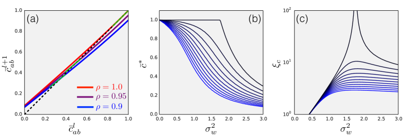
Figure 3: Dropout destroys the critical point, and limits the depth to which information can propagate in a deep network. (a) The iterative correlation map showing c¯abl+1subscriptsuperscript¯𝑐𝑙1𝑎𝑏\bar{c}^{l+1}_{ab} as a function of c¯ablsubscriptsuperscript¯𝑐𝑙𝑎𝑏\bar{c}^{l}_{ab} for three different values of the dropout rate ρ𝜌\rho for networks tuned close to their critical point. Green inset lines show the linearization of the iterative map about the critical point, e1/ξcsuperscript𝑒1subscript𝜉𝑐e^{-1/\xi_{c}}. (b) The asymptotic value of the correlation map, csuperscript𝑐c^{*}, as a function of σw2superscriptsubscript𝜎𝑤2\sigma_{w}^{2} for different values of dropout from ρ=1𝜌1\rho=1 (black) to ρ=0.8𝜌0.8\rho=0.8 (blue). We see that for all values of dropout except for ρ=1𝜌1\rho=1, csuperscript𝑐c^{*} does not show a sharp transition between an ordered phase and a chaotic phase. (c) The correlation depth scale ξcsubscript𝜉𝑐\xi_{c} as a function of σw2superscriptsubscript𝜎𝑤2\sigma_{w}^{2} for the same values of dropout as in (b). We see here that for all values of ρ𝜌\rho except for ρ=1𝜌1\rho=1 there is no divergence in ξcsubscript𝜉𝑐\xi_{c}.

As in networks without dropout we plot, in fig. 3 (a), the iterative map c¯abl+1subscriptsuperscript¯𝑐𝑙1𝑎𝑏\bar{c}^{l+1}_{ab} as a function of c¯ablsubscriptsuperscript¯𝑐𝑙𝑎𝑏\bar{c}^{l}_{ab}. Most significantly, we see that the c¯abl=1subscriptsuperscript¯𝑐𝑙𝑎𝑏1\bar{c}^{l}_{ab}=1 is no longer a fixed point of the dynamics. Instead, as the dropout rate increases c¯ablsubscriptsuperscript¯𝑐𝑙𝑎𝑏\bar{c}^{l}_{ab} gets mapped to decreasing values and the fixed point monotonically decreases.

To test these results we plot in fig. 3 (b) the asymptotic correlation, csuperscript𝑐c^{*}, as a function of σw2superscriptsubscript𝜎𝑤2\sigma_{w}^{2} for different values of dropout from ρ=0.8𝜌0.8\rho=0.8 to ρ=1.0𝜌1.0\rho=1.0. As expected, we see that for all ρ<1𝜌1\rho<1 there is no sharp transition between c=1superscript𝑐1c^{*}=1 and c<1superscript𝑐1c^{*}<1. Moreover as the dropout rate increases the correlation csuperscript𝑐c^{*} monotonically decreases. Intuitively this makes sense. Identical inputs passed through two different dropout masks will become increasingly dissimilar as the dropout rate increases. In fig. 3 (c) we show the depth scale, ξcsubscript𝜉𝑐\xi_{c}, as a function of σw2superscriptsubscript𝜎𝑤2\sigma_{w}^{2} for the same range of dropout probabilities. We find that, as predicted, the depth of signal propagation with dropout is drastically reduced and, importantly, there is no longer a divergence in ξcsubscript𝜉𝑐\xi_{c}. Increasing the dropout rate continues to decrease the correlation depth for constant σw2superscriptsubscript𝜎𝑤2\sigma_{w}^{2}.

4 Gradient Backpropagation

There is a duality between the forward propagation of signals and the backpropagation of gradients. To elucidate this connection consider the backpropagation equations given a loss E𝐸E,

EWijl=δilϕ(zjl1)δil=ϕ(zil)jδjl+1Wjil+1formulae-sequence𝐸superscriptsubscript𝑊𝑖𝑗𝑙superscriptsubscript𝛿𝑖𝑙italic-ϕsuperscriptsubscript𝑧𝑗𝑙1superscriptsubscript𝛿𝑖𝑙superscriptitalic-ϕsuperscriptsubscript𝑧𝑖𝑙subscript𝑗superscriptsubscript𝛿𝑗𝑙1superscriptsubscript𝑊𝑗𝑖𝑙1\frac{\partial E}{\partial W_{ij}^{l}}=\delta_{i}^{l}\phi(z_{j}^{l-1})\hskip 60.0pt\delta_{i}^{l}=\phi^{\prime}(z_{i}^{l})\sum_{j}\delta_{j}^{l+1}W_{ji}^{l+1} (14)

with the identification δil=E/zilsubscriptsuperscript𝛿𝑙𝑖𝐸superscriptsubscript𝑧𝑖𝑙\delta^{l}_{i}=\partial E/\partial z_{i}^{l}. Within mean field theory, it is clear that the scale of fluctuations of the gradient of weights in a layer will be proportional to 𝔼[(δil)2]𝔼delimited-[]superscriptsubscriptsuperscript𝛿𝑙𝑖2\mathbb{E}[(\delta^{l}_{i})^{2}] (see appendix 7.6). In contrast to the pre-activations in forward propagation (eq. 1), the δilsubscriptsuperscript𝛿𝑙𝑖\delta^{l}_{i} will typically not be Gaussian distributed even in the large layer width limit.

Nonetheless, we can work out a recurrence relation for the variance of the error, q~aal=𝔼[(δil)2]superscriptsubscript~𝑞𝑎𝑎𝑙𝔼delimited-[]superscriptsubscriptsuperscript𝛿𝑙𝑖2\tilde{q}_{aa}^{\ l}=\mathbb{E}[(\delta^{l}_{i})^{2}], leveraging the Gaussian ansatz on the pre-activations. In order to do this, however, we must first make an additional approximation that the weights used during forward propagation are drawn independently from the weights used in backpropagation. This approximation is similar in spirit to the vanilla mean field approximation and is reminiscent of work on feedback alignment (Lillicrap et al., 2014). With this in mind we arrive at the recurrence (see appendix 7.7),

q~aal=q~aal+1Nl+1Nlχ1.superscriptsubscript~𝑞𝑎𝑎𝑙superscriptsubscript~𝑞𝑎𝑎𝑙1subscript𝑁𝑙1subscript𝑁𝑙subscript𝜒1\tilde{q}_{aa}^{\ l}=\tilde{q}_{aa}^{\ l+1}\frac{N_{l+1}}{N_{l}}\chi_{1}. (15)

The presence of χ1subscript𝜒1\chi_{1} in the above equation should perhaps not be surprising. In Poole et al. (2016) they show that χ1subscript𝜒1\chi_{1} is intimately related to the tangent space of a given layer in mean field neural networks. We note that the backpropagation recurrence features an explicit dependence on the ratio of widths of adjacent layers of the network, Nl+1/Nlsubscript𝑁𝑙1subscript𝑁𝑙N_{l+1}/N_{l}. Here we will consider exclusively constant width networks where this factor is unity. For a discussion of the case of unequal layer widths see Glorot & Bengio (2010).

Since χ1subscript𝜒1\chi_{1} depends only on the asymptotic qsuperscript𝑞q^{*} it follows that for constant width networks we expect eq. 15 to again have an exponential solution with,

q~aal=q~aaLe(Ll)/ξξ1=logχ1.formulae-sequencesuperscriptsubscript~𝑞𝑎𝑎𝑙superscriptsubscript~𝑞𝑎𝑎𝐿superscript𝑒𝐿𝑙subscript𝜉superscriptsubscript𝜉1subscript𝜒1\tilde{q}_{aa}^{\ l}=\tilde{q}_{aa}^{\ L}e^{-(L-l)/\xi_{{}_{\nabla}}}\hskip 48.0pt\xi_{{}_{\nabla}}^{-1}=-\log\chi_{1}. (16)

Note that here ξ1=logχ1superscriptsubscript𝜉1subscript𝜒1\xi_{{}_{\nabla}}^{-1}=-\log\chi_{1} both above and below the transition. It follows that ξsubscript𝜉\xi_{{}_{\nabla}} can be both positive and negative. We conclude that there should be three distinct regimes for the gradients.

  1. 1.

    In the ordered phase, χ1<1subscript𝜒11\chi_{1}<1 and so ξ>0subscript𝜉0\xi_{{}_{\nabla}}>0. We therefore expect gradients to vanish over a depth |ξ|subscript𝜉|\xi_{{}_{\nabla}}|.

  2. 2.

    At criticality, χ11subscript𝜒11\chi_{1}\to 1 and so ξsubscript𝜉\xi_{{}_{\nabla}}\to\infty. Here gradients should be stable regardless of depth.

  3. 3.

    In the chaotic phase, χ1>1subscript𝜒11\chi_{1}>1 and so ξ<0subscript𝜉0\xi_{{}_{\nabla}}<0. It follows that in this regime gradients should explode over a depth |ξ|subscript𝜉|\xi_{{}_{\nabla}}|.

Intuitively these three regimes make sense. To see this, recall that perturbations to a weight in layer l𝑙l can alternatively be viewed as perturbations to the pre-activations in the same layer. In the ordered phase both the perturbed signal and the unperturbed signal will be asymptotically mapped to the same point and the derivative will be small. In the chaotic phase the perturbed and unperturbed signals will become asymptotically decorrelated and the gradient will be large.
Refer to caption
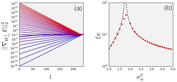
Figure 4: Gradient backpropagation behaves similarly to signal forward propagation. (a) The 2-norm, WablE22superscriptsubscriptnormsubscriptsuperscriptsubscript𝑊𝑎𝑏𝑙𝐸22||\nabla_{W_{ab}^{l}}E||_{2}^{2} as a function of layer, l𝑙l, for a 240 layer random network with a cross-entropy loss on MNIST. Different values of σw2superscriptsubscript𝜎𝑤2\sigma_{w}^{2} from 1.0 (blue) to 4.0 (red) are shown. Clear exponential vanishing / explosion is observed over many orders of magnitude. (b) The depth scale for gradients predicted by theory (dashed line) compared with measurements from experiment (red dots). Similarity between theory and experiment is clear. Deviations near the critical point are primarily due to finite size effects.

To investigate these predictions we construct deep random networks of depth L=240𝐿240L=240 and layer-width Nl=300subscript𝑁𝑙300N_{l}=300. We then consider the cross-entropy loss of these networks on MNIST. In fig. 4 (a) we plot the layer-by-layer 2-norm of the gradient, WablE22superscriptsubscriptnormsubscriptsuperscriptsubscript𝑊𝑎𝑏𝑙𝐸22||\nabla_{W_{ab}^{l}}E||_{2}^{2}, as a function of layer, l𝑙l, for different values of σw2superscriptsubscript𝜎𝑤2\sigma_{w}^{2}. We see that WablE22superscriptsubscriptnormsubscriptsuperscriptsubscript𝑊𝑎𝑏𝑙𝐸22||\nabla_{W_{ab}^{l}}E||_{2}^{2} behaves exponentially over many orders of magnitude. Moreover, we see that the gradient vanishes in the ordered phase and explodes in the chaotic phase. We test the quantitative predictions of eq. 16 in fig. 4 (b) where we compare |ξ|subscript𝜉|\xi_{{}_{\nabla}}| as predicted from theory with the measured depth-scale constructed from exponential fits to the gradient data. Here we see good quantitative agreement between the theoretical predictions from mean field random networks and experimentally realized networks. Together these results suggest that the approximations on the backpropagation equations were representative of deep, wide, random networks.

Finally, we show that the depth scale for correlated signal propagation likewise controls the depth at which information stored in the covariance between gradients can survive. The existence of consistent gradients across similar samples from a training set ought to be especially important for determining whether or not a given neural network architecture can be trained. To establish this depth-scale first note (see Appendix 7.8) that the covariance between gradients of two different inputs, xi;1subscript𝑥𝑖1x_{i;1} and xi;2subscript𝑥𝑖2x_{i;2}, will be proportional to (WijlEa)(WijlEb)𝔼[δi;alδi;bl]=q~ablsimilar-tosubscriptsuperscriptsubscript𝑊𝑖𝑗𝑙subscript𝐸𝑎subscriptsuperscriptsubscript𝑊𝑖𝑗𝑙subscript𝐸𝑏𝔼delimited-[]superscriptsubscript𝛿𝑖𝑎𝑙superscriptsubscript𝛿𝑖𝑏𝑙superscriptsubscript~𝑞𝑎𝑏𝑙(\nabla_{W_{ij}^{l}}E_{a})\cdot(\nabla_{W_{ij}^{l}}E_{b})\sim\mathbb{E}[\delta_{i;a}^{l}\delta_{i;b}^{l}]=\tilde{q}_{ab}^{\ l} where Easubscript𝐸𝑎E_{a} is the loss evaluated on xi;asubscript𝑥𝑖𝑎x_{i;a} and δi;a=Ea/zi;alsubscript𝛿𝑖𝑎subscript𝐸𝑎superscriptsubscript𝑧𝑖𝑎𝑙\delta_{i;a}=\partial E_{a}/\partial z_{i;a}^{l} are appropriately defined errors.

It can be shown (see Appendix 7.9) that q~ablsuperscriptsubscript~𝑞𝑎𝑏𝑙\tilde{q}_{ab}^{\ l} features the recurrence relation,

q~abl=q~abl+1Nl+1Nl+2σw2𝒟z1𝒟z2ϕ(u1)ϕ(u2)superscriptsubscript~𝑞𝑎𝑏𝑙superscriptsubscript~𝑞𝑎𝑏𝑙1subscript𝑁𝑙1subscript𝑁𝑙2superscriptsubscript𝜎𝑤2𝒟subscript𝑧1𝒟subscript𝑧2superscriptitalic-ϕsubscript𝑢1superscriptitalic-ϕsubscript𝑢2\tilde{q}_{ab}^{\ l}=\tilde{q}_{ab}^{\ l+1}\frac{N_{l+1}}{N_{l+2}}\sigma_{w}^{2}\int\mathcal{D}z_{1}\mathcal{D}z_{2}\phi^{\prime}(u_{1})\phi^{\prime}(u_{2}) (17)

where u1subscript𝑢1u_{1} and u2subscript𝑢2u_{2} are defined similarly as for the forward pass. Expanding asymptotically it is clear that to zeroth order in ϵlsuperscriptitalic-ϵ𝑙\epsilon^{l}, q~ablsuperscriptsubscript~𝑞𝑎𝑏𝑙\tilde{q}_{ab}^{l} will have an exponential solution with q~abl=q~abLe(Ll)/ξcsuperscriptsubscript~𝑞𝑎𝑏𝑙superscriptsubscript~𝑞𝑎𝑏𝐿superscript𝑒𝐿𝑙subscript𝜉𝑐\tilde{q}_{ab}^{\ l}=\tilde{q}_{ab}^{\ L}e^{-(L-l)/\xi_{c}} with ξcsubscript𝜉𝑐\xi_{c} as defined in the forward pass.

5 Experimental Results

Taken together, the results of this paper lead us to the following hypothesis: a necessary condition for a random network to be trained is that information about the inputs should be able to propagate forward through the network, and information about the gradients should be able to propagate backwards through the network. The preceding analysis shows that networks will have this property precisely when the network depth, L𝐿L, is not much larger than the depth-scale ξcsubscript𝜉𝑐\xi_{c}. This criterion is data independent and therefore offers a “universal” constraint on the hyperparameters that depends on network architecture alone. We now explore this relationship between depth of signal propagation and network trainability empirically.
Refer to caption
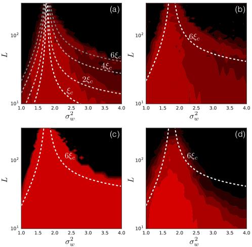
Figure 5: Mean field depth scales control trainable hyperparameters. The training accuracy for neural networks as a function of their depth and initial weight variance, σw2superscriptsubscript𝜎𝑤2\sigma_{w}^{2} from a high accuracy (red) to low accuracy (black). In (a) we plot the training accuracy after 200 training steps on MNIST using SGD. Here overlayed in grey dashed lines are different multiples of the depth scale for correlated signal propagation, nξc𝑛subscript𝜉𝑐n\xi_{c}. We plot the accuracy in (b) after 2000 training steps on CIFAR10 using SGD, in (c) after 14000 training steps on MNIST using SGD, and in (d) after 300 training steps on MNIST using RMSPROP. Here we overlay in white dashed lines 6ξc6subscript𝜉𝑐6\xi_{c}.

To investigate this prediction, we consider random networks of depth 10L30010𝐿30010\leq L\leq 300 and 1σw241superscriptsubscript𝜎𝑤241\leq\sigma_{w}^{2}\leq 4 with σb2=0.05superscriptsubscript𝜎𝑏20.05\sigma_{b}^{2}=0.05. We train these networks using Stochastic Gradient Descent (SGD) and RMSProp on MNIST and CIFAR10. We use a learning rate of 103superscript10310^{-3} for SGD when L200less-than-or-similar-to𝐿200L\lesssim 200, 104superscript10410^{-4} for larger L𝐿L, and 105superscript10510^{-5} for RMSProp. These learning rates were selected by grid search between 106superscript10610^{-6} and 102superscript10210^{-2} in exponentially spaced steps of size 101010. We note that the depth dependence of learning rate was explored in detail in Saxe et al. (2014). In fig. 5 (a)-(d) we color in red the training accuracy that neural networks achieved as a function of σw2superscriptsubscript𝜎𝑤2\sigma_{w}^{2} and L𝐿L for different datasets, training time, and choice of minimizer (see Appendix 7.10 for more comparisons). In all cases the neural networks over-fit the data to give a training accuracy of 100%percent100100\% and test accuracies of 98%percent9898\% on MNIST and 55%percent5555\% on CIFAR10. We emphasize that the purpose of this study is to demonstrate trainability as opposed to optimizing test accuracy.

We now make the connection between the depth scale, ξcsubscript𝜉𝑐\xi_{c}, and the maximum trainable depth more precise. Given the arguments in the preceding sections we note that if L=nξc𝐿𝑛subscript𝜉𝑐L=n\xi_{c} then signal through the network will be attenuated by a factor of ensuperscript𝑒𝑛e^{n}. To understand how much signal can be lost while still allowing for training, we overlay in fig. 5 (a) curves corresponding to nξc𝑛subscript𝜉𝑐n\xi_{c} from n=1𝑛1n=1 to 666. We find that networks appear to be trainable when L6ξcless-than-or-similar-to𝐿6subscript𝜉𝑐L\lesssim 6\xi_{c}. It would be interesting to understand why this is the case.

Motivated by this argument in fig. 5 (b)-(d) in white, dashed, overlay we plot twice the predicted depth scale, 6ξc6subscript𝜉𝑐6\xi_{c}. There is clearly a relationship between the depth of correlated signal propagation and whether or not these networks are trainable. Networks closer to their critical point appear to train more quickly than those further away. Moreover, this relationship has no obvious dependence on dataset, duration of training, or minimizer. We therefore conclude that these bounds on trainable hyperparameters are universal. This in turn implies that to train increasingly deep networks, one must generically be ever closer to criticality.
Refer to caption
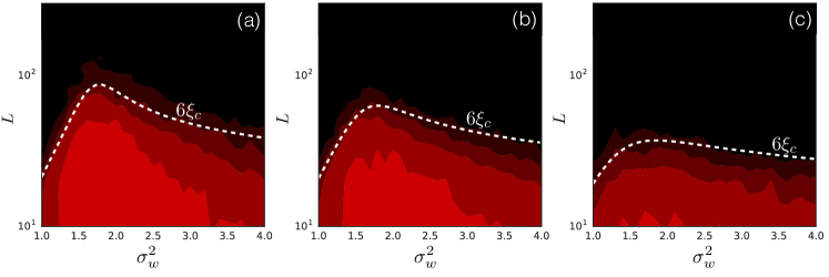
Figure 6: The effect of dropout on trainability. The same scheme as in fig. 5 but with dropout rates of (a) ρ=0.99𝜌0.99\rho=0.99, (b) ρ=0.98𝜌0.98\rho=0.98, and (c) ρ=0.94𝜌0.94\rho=0.94. Even for modest amounts of dropout we see an upper bound on the maximum trainable depth for neural networks. We continue to see good agreement between the prediction of our theory and our experimental training accuracy.

Next we consider the effect of dropout. As we showed earlier, even infinitesimal amounts of dropout disrupt the order-to-chaos phase transition and cause the depth scale to become finite. However, since the effect of a single dropout mask is to simply re-scale the weight variance by σw2σw2/ρsuperscriptsubscript𝜎𝑤2superscriptsubscript𝜎𝑤2𝜌\sigma_{w}^{2}\to\sigma_{w}^{2}/\rho, the gradient magnitude will be stable near criticality, while the input and gradient correlations will not be. This therefore offers a unique opportunity to test whether the relevant depth-scale is |1/logχ1|1subscript𝜒1|1/\log\chi_{1}| or ξcsubscript𝜉𝑐\xi_{c}.

In fig. 6 we repeat the same experimental setup as above on MNIST with dropout rates ρ=0.99,0.98,𝜌0.990.98\rho=0.99,0.98, and 0.94. We observe, first and foremost, that even extremely modest amounts of dropout limit the maximum trainable depth to about L=100𝐿100L=100. We additionally notice that the depth-scale, ξcsubscript𝜉𝑐\xi_{c}, predicts the trainable region accurately for varying amounts of dropout.

6 Discussion

In this paper we have elucidated the existence of several depth-scales that control signal propagation in random neural networks. Furthermore, we have shown that the degree to which a neural network can be trained depends crucially on its ability to propagate information about inputs and gradients through its full depth. At the transition between order and chaos, information stored in the correlation between inputs can propagate infinitely far through these random networks. This in turn implies that extremely deep neural networks may be trained sufficiently close to criticality. However, our contribution goes beyond advocating for hyperparameter selection that brings random networks to be nearly critical. Instead, we offer a general purpose framework that predicts, at the level of mean field theory, which hyperparameters should allow a network to be trained. This is especially relevant when analyzing schemes like dropout where there is no critical point and which therefore imply an upper bound on trainable network depth.

An alternative perspective as to why information stored in the covariance between inputs is crucial for training can be understood by appealing to the correspondence between infinitely wide Bayesian neural networks and Gaussian Processes (Neal, 2012). In particular the covariance, qablsuperscriptsubscript𝑞𝑎𝑏𝑙q_{ab}^{l}, is intimately related to the kernel of the induced Gaussian Process. It follows that cases in which signal stored in the covariance between inputs may propagate through the network correspond precisely to situations in which the associated Gaussian Process is well defined.

Our work suggests that it may be fruitful to investigate pre-training schemes that attempt to perturb the weights of a neural network to favor information flow through the network. In principle this could be accomplished through a layer-by-layer local criterion for information flow or by selecting the mean and variance in schemes like batch normalization to maximize the covariance depth-scale.

These results suggest that theoretical work on random neural networks can be used to inform practical architectural decisions. However, there is still much work to be done. For instance, the framework developed here does not apply to unbounded activations, such as rectified linear units, where it can be shown that there are phases in which eq. 3 does not have a fixed point. Additionally, the analysis here applies directly only to fully connected feed-forward networks, and will need to be extended to architectures with structured weight matrices such as convolutional networks.

We close by noting that in physics it has long been known that, through renormalization, the behavior of systems near critical points can control their behavior even far from the idealized critical case. We therefore make the somewhat bold hypothesis that a broad class of neural network topologies will be controlled by the fully-connected mean field critical point.

Acknowledgments

We thank Ben Poole, Jeffrey Pennington, Maithra Raghu, and George Dahl for useful discussions. We are additionally grateful to RocketAI for introducing us to Temporally Recurrent Online Learning and two-dimensional time.

References

  • Bengio et al. (1993) Y Bengio, Paolo Frasconi, and P Simard. The problem of learning long-term dependencies in recurrent networks. In Neural Networks, 1993., IEEE International Conference on, pp.  1183–1188. IEEE, 1993.
  • Bertschinger et al. (2005) Nils Bertschinger, Thomas Natschläger, and Robert A. Legenstein. At the edge of chaos: Real-time computations and self-organized criticality in recurrent neural networks. In L. K. Saul, Y. Weiss, and L. Bottou (eds.), Advances in Neural Information Processing Systems 17, pp.  145–152. MIT Press, 2005.
  • Choromanska et al. (2015) Anna Choromanska, Mikael Henaff, Michael Mathieu, Gérard Ben Arous, and Yann LeCun. The loss surfaces of multilayer networks. In AISTATS, 2015.
  • Daniely et al. (2016) A. Daniely, R. Frostig, and Y. Singer. Toward Deeper Understanding of Neural Networks: The Power of Initialization and a Dual View on Expressivity. arXiv:1602.05897, 2016.
  • Glorot & Bengio (2010) Xavier Glorot and Yoshua Bengio. Understanding the difficulty of training deep feedforward neural networks. In Aistats, volume 9, pp.  249–256, 2010.
  • Goodfellow et al. (2014) Ian J Goodfellow, Oriol Vinyals, and Andrew M Saxe. Qualitatively characterizing neural network optimization problems. arXiv:1412.6544, 2014.
  • He et al. (2015) K. He, X. Zhang, S. Ren, and J. Sun. Deep Residual Learning for Image Recognition. ArXiv e-prints, December 2015.
  • Ioffe & Szegedy (2015) Sergey Ioffe and Christian Szegedy. Batch normalization: Accelerating deep network training by reducing internal covariate shift. In Proceedings of The 32nd International Conference on Machine Learning, pp.  448–456, 2015.
  • Lillicrap et al. (2014) Timothy P Lillicrap, Daniel Cownden, Douglas B Tweed, and Colin J Akerman. Random feedback weights support learning in deep neural networks. arXiv:1411.0247, 2014.
  • Montufar et al. (2014) Guido F Montufar, Razvan Pascanu, Kyunghyun Cho, and Yoshua Bengio. On the number of linear regions of deep neural networks. In Z. Ghahramani, M. Welling, C. Cortes, N. D. Lawrence, and K. Q. Weinberger (eds.), Advances in Neural Information Processing Systems 27, pp.  2924–2932. Curran Associates, Inc., 2014.
  • Neal (2012) Radford M Neal. Bayesian learning for neural networks, volume 118. Springer Science & Business Media, 2012.
  • Poole et al. (2016) B. Poole, S. Lahiri, M. Raghu, J. Sohl-Dickstein, and S. Ganguli. Exponential expressivity in deep neural networks through transient chaos. arXiv:1606.05340, June 2016.
  • Raghu et al. (2016) M. Raghu, B. Poole, J. Kleinberg, S. Ganguli, and J. Sohl-Dickstein. On the expressive power of deep neural networks. arXiv:1606.05336, June 2016.
  • Recht et al. (2015) Benjamin Recht, Moritz Hardt, and Yoram Singer. Train faster, generalize better: Stability of stochastic gradient descent. arXiv:1509.01240, 2015.
  • Saxe et al. (2014) A. M. Saxe, J. L. McClelland, and S. Ganguli. Exact solutions to the nonlinear dynamics of learning in deep linear neural networks. International Conference on Learning Representations, 2014.
  • Sussillo & Abbott (2014) David Sussillo and LF Abbott. Random walks: Training very deep nonlinear feed-forward networks with smart initialization. CoRR, vol. abs/1412.6558, 2014.

7 Appendix

Here we present derivations of results from throughout the paper.

7.1 Single input depth-scale

Result:

Consider the recurrence relation for the variance of a single input,

qaal=σw2𝒟zϕ2(qaal1z)+σb2superscriptsubscript𝑞𝑎𝑎𝑙superscriptsubscript𝜎𝑤2𝒟𝑧superscriptitalic-ϕ2superscriptsubscript𝑞𝑎𝑎𝑙1𝑧superscriptsubscript𝜎𝑏2q_{aa}^{l}=\sigma_{w}^{2}\int\mathcal{D}z\phi^{2}\left(\sqrt{q_{aa}^{l-1}}z\right)+\sigma_{b}^{2} (18)

and a fixed point of the dynamics, qsuperscript𝑞q^{*}. qaalsubscriptsuperscript𝑞𝑙𝑎𝑎q^{l}_{aa} can be expanded about the fixed point to yield the asymptotic recurrence relation,

ϵl+1=ϵl[χ1+σw2𝒟zϕ′′(qz)ϕ(qz)]+𝒪((ϵl)2).superscriptitalic-ϵ𝑙1superscriptitalic-ϵ𝑙delimited-[]subscript𝜒1superscriptsubscript𝜎𝑤2𝒟𝑧superscriptitalic-ϕ′′superscript𝑞𝑧italic-ϕsuperscript𝑞𝑧𝒪superscriptsuperscriptitalic-ϵ𝑙2\epsilon^{l+1}=\epsilon^{l}\left[\chi_{1}+\sigma_{w}^{2}\int\mathcal{D}z\phi^{\prime\prime}\left(\sqrt{q^{*}}z\right)\phi\left(\sqrt{q^{*}}z\right)\right]+\mathcal{O}\left((\epsilon^{l})^{2}\right). (19)

Derivation:

We begin by first expanding to order ϵlsuperscriptitalic-ϵ𝑙\epsilon^{l},

q+ϵl+1superscript𝑞superscriptitalic-ϵ𝑙1\displaystyle q^{*}+\epsilon^{l+1} =σw2𝒟z[ϕ(q+ϵlz)]2+σb2absentsuperscriptsubscript𝜎𝑤2𝒟𝑧superscriptdelimited-[]italic-ϕsuperscript𝑞superscriptitalic-ϵ𝑙𝑧2superscriptsubscript𝜎𝑏2\displaystyle=\sigma_{w}^{2}\int\mathcal{D}z\left[\phi\left(\sqrt{q^{*}+\epsilon^{l}}z\right)\right]^{2}+\sigma_{b}^{2} (20)
σw2𝒟z[ϕ(qz+12ϵlzq)]2+σb2absentsuperscriptsubscript𝜎𝑤2𝒟𝑧superscriptdelimited-[]italic-ϕsuperscript𝑞𝑧12superscriptitalic-ϵ𝑙𝑧superscript𝑞2superscriptsubscript𝜎𝑏2\displaystyle\approx\sigma_{w}^{2}\int\mathcal{D}z\left[\phi\left(\sqrt{q^{*}}z+\frac{1}{2}\frac{\epsilon^{l}z}{\sqrt{q^{*}}}\right)\right]^{2}+\sigma_{b}^{2} (21)
σw2𝒟z[ϕ(qz)+12ϵlzqϕ(qz)]2+σb2+𝒪((ϵl)2)absentsuperscriptsubscript𝜎𝑤2𝒟𝑧superscriptdelimited-[]italic-ϕsuperscript𝑞𝑧12superscriptitalic-ϵ𝑙𝑧superscript𝑞superscriptitalic-ϕsuperscript𝑞𝑧2superscriptsubscript𝜎𝑏2𝒪superscriptsuperscriptitalic-ϵ𝑙2\displaystyle\approx\sigma_{w}^{2}\int\mathcal{D}z\left[\phi\left(\sqrt{q^{*}}z\right)+\frac{1}{2}\frac{\epsilon^{l}z}{\sqrt{q^{*}}}\phi^{\prime}\left(\sqrt{q^{*}}z\right)\right]^{2}+\sigma_{b}^{2}+\mathcal{O}((\epsilon^{l})^{2}) (22)
σw2𝒟zϕ2(qz)+σb2+ϵlσw2q𝒟zzϕ(qz)ϕ(qz)+𝒪((ϵl)2)absentsuperscriptsubscript𝜎𝑤2𝒟𝑧superscriptitalic-ϕ2superscript𝑞𝑧superscriptsubscript𝜎𝑏2superscriptitalic-ϵ𝑙superscriptsubscript𝜎𝑤2superscript𝑞𝒟𝑧𝑧italic-ϕsuperscript𝑞𝑧superscriptitalic-ϕsuperscript𝑞𝑧𝒪superscriptsuperscriptitalic-ϵ𝑙2\displaystyle\approx\sigma_{w}^{2}\int\mathcal{D}z\phi^{2}\left(\sqrt{q^{*}}z\right)+\sigma_{b}^{2}+\epsilon^{l}\frac{\sigma_{w}^{2}}{\sqrt{q^{*}}}\int\mathcal{D}zz\phi\left(\sqrt{q^{*}}z\right)\phi^{\prime}\left(\sqrt{q^{*}}z\right)+\mathcal{O}((\epsilon^{l})^{2}) (23)
q+ϵlσw2q𝒟zzϕ(qz)ϕ(qz)+𝒪((ϵl)2).absentsuperscript𝑞superscriptitalic-ϵ𝑙superscriptsubscript𝜎𝑤2superscript𝑞𝒟𝑧𝑧italic-ϕsuperscript𝑞𝑧superscriptitalic-ϕsuperscript𝑞𝑧𝒪superscriptsuperscriptitalic-ϵ𝑙2\displaystyle\approx q^{*}+\epsilon^{l}\frac{\sigma_{w}^{2}}{\sqrt{q^{*}}}\int\mathcal{D}zz\phi(\sqrt{q^{*}}z)\phi^{\prime}\left(\sqrt{q^{*}}z\right)+\mathcal{O}((\epsilon^{l})^{2}). (24)

We therefore arrive at the approximate reccurence relation,

ϵl+1=ϵlσw2q𝒟zzϕ(qz)ϕ(qz)+𝒪((ϵl)2).superscriptitalic-ϵ𝑙1superscriptitalic-ϵ𝑙superscriptsubscript𝜎𝑤2superscript𝑞𝒟𝑧𝑧italic-ϕsuperscript𝑞𝑧superscriptitalic-ϕsuperscript𝑞𝑧𝒪superscriptsuperscriptitalic-ϵ𝑙2\epsilon^{l+1}=\epsilon^{l}\frac{\sigma_{w}^{2}}{\sqrt{q^{*}}}\int\mathcal{D}zz\phi(\sqrt{q^{*}}z)\phi^{\prime}\left(\sqrt{q^{*}}z\right)+\mathcal{O}((\epsilon^{l})^{2}). (25)

Using the identity, 𝒟zzf(z)=𝒟zf(z)𝒟𝑧𝑧𝑓𝑧𝒟𝑧superscript𝑓𝑧\int\mathcal{D}zzf(z)=\int\mathcal{D}zf^{\prime}(z) we can rewrite this asymptotic recurrence relation as,

ϵl+1superscriptitalic-ϵ𝑙1\displaystyle\epsilon^{l+1} =ϵl[σw2𝒟z[ϕ(qz)]2+σw2𝒟zϕ′′(qz)ϕ(qz)]+𝒪((ϵl)2)absentsuperscriptitalic-ϵ𝑙delimited-[]superscriptsubscript𝜎𝑤2𝒟𝑧superscriptdelimited-[]superscriptitalic-ϕsuperscript𝑞𝑧2superscriptsubscript𝜎𝑤2𝒟𝑧superscriptitalic-ϕ′′superscript𝑞𝑧italic-ϕsuperscript𝑞𝑧𝒪superscriptsuperscriptitalic-ϵ𝑙2\displaystyle=\epsilon^{l}\left[\sigma_{w}^{2}\int\mathcal{D}z\left[\phi^{\prime}\left(\sqrt{q^{*}}z\right)\right]^{2}+\sigma_{w}^{2}\int\mathcal{D}z\phi^{\prime\prime}\left(\sqrt{q^{*}}z\right)\phi\left(\sqrt{q^{*}}z\right)\right]+\mathcal{O}((\epsilon^{l})^{2}) (26)
=ϵl[χ1+σw2𝒟zϕ′′(qz)ϕ(qz)]+𝒪((ϵl)2)absentsuperscriptitalic-ϵ𝑙delimited-[]subscript𝜒1superscriptsubscript𝜎𝑤2𝒟𝑧superscriptitalic-ϕ′′superscript𝑞𝑧italic-ϕsuperscript𝑞𝑧𝒪superscriptsuperscriptitalic-ϵ𝑙2\displaystyle=\epsilon^{l}\left[\chi_{1}+\sigma_{w}^{2}\int\mathcal{D}z\phi^{\prime\prime}\left(\sqrt{q^{*}}z\right)\phi\left(\sqrt{q^{*}}z\right)\right]+\mathcal{O}((\epsilon^{l})^{2}) (27)

as required.

7.2 Two input depth-scale

Result:

Consider the recurrence relation for the co-variance of two input,

qabl=σw2𝒟z1𝒟z2ϕ(u1)ϕ(u2)+σb2,superscriptsubscript𝑞𝑎𝑏𝑙superscriptsubscript𝜎𝑤2𝒟subscript𝑧1𝒟subscript𝑧2italic-ϕsubscript𝑢1italic-ϕsubscript𝑢2superscriptsubscript𝜎𝑏2q_{ab}^{l}=\sigma_{w}^{2}\int\mathcal{D}z_{1}\mathcal{D}z_{2}\phi(u_{1})\phi(u_{2})+\sigma_{b}^{2}, (28)

a correlation between the inputs, cabl=qabl/qaalqbblsuperscriptsubscript𝑐𝑎𝑏𝑙superscriptsubscript𝑞𝑎𝑏𝑙superscriptsubscript𝑞𝑎𝑎𝑙superscriptsubscript𝑞𝑏𝑏𝑙c_{ab}^{l}=q_{ab}^{l}/\sqrt{q_{aa}^{l}q_{bb}^{l}}, and a fixed point of the dynamics, csuperscript𝑐c^{*}. cablsubscriptsuperscript𝑐𝑙𝑎𝑏c^{l}_{ab} can be expanded about the fixed point to yield the asymptotic recurrence relation,

ϵl+1=ϵl[σw2𝒟z1𝒟z2ϕ(u1)ϕ(u2)]+𝒪((ϵl)2).superscriptitalic-ϵ𝑙1superscriptitalic-ϵ𝑙delimited-[]superscriptsubscript𝜎𝑤2𝒟subscript𝑧1𝒟subscript𝑧2superscriptitalic-ϕsubscript𝑢1superscriptitalic-ϕsubscript𝑢2𝒪superscriptsuperscriptitalic-ϵ𝑙2\epsilon^{l+1}=\epsilon^{l}\left[\sigma_{w}^{2}\int\mathcal{D}z_{1}\mathcal{D}z_{2}\phi^{\prime}(u_{1})\phi^{\prime}(u_{2})\right]+\mathcal{O}\left((\epsilon^{l})^{2}\right). (29)

Derivation:

Since the relaxation of qaalsubscriptsuperscript𝑞𝑙𝑎𝑎q^{l}_{aa} and qbblsubscriptsuperscript𝑞𝑙𝑏𝑏q^{l}_{bb} to qsuperscript𝑞q^{*} occurs much more quickly than the convergence of qablsuperscriptsubscript𝑞𝑎𝑏𝑙q_{ab}^{l} we approximate qaal=qbbl=qsubscriptsuperscript𝑞𝑙𝑎𝑎subscriptsuperscript𝑞𝑙𝑏𝑏superscript𝑞q^{l}_{aa}=q^{l}_{bb}=q^{*} as in Poole et al. (2016). We therefore consider the perturbation qabl/q=cabl=c+ϵlsuperscriptsubscript𝑞𝑎𝑏𝑙superscript𝑞superscriptsubscript𝑐𝑎𝑏𝑙superscript𝑐superscriptitalic-ϵ𝑙q_{ab}^{l}/q^{*}=c_{ab}^{l}=c^{*}+\epsilon^{l}. It follows that we may make the approximation,

u2lsuperscriptsubscript𝑢2𝑙\displaystyle u_{2}^{l} =q(cablz1+1(cabl)2z2)absentsuperscript𝑞superscriptsubscript𝑐𝑎𝑏𝑙subscript𝑧11superscriptsuperscriptsubscript𝑐𝑎𝑏𝑙2subscript𝑧2\displaystyle=\sqrt{q^{*}}\left(c_{ab}^{l}z_{1}+\sqrt{1-(c_{ab}^{l})^{2}}z_{2}\right) (30)
q(cz1+1(c)22cϵlz2)+qϵlz1+𝒪(ϵ2)absentsuperscript𝑞superscript𝑐subscript𝑧11superscriptsuperscript𝑐22superscript𝑐superscriptitalic-ϵ𝑙subscript𝑧2superscript𝑞superscriptitalic-ϵ𝑙subscript𝑧1𝒪superscriptitalic-ϵ2\displaystyle\approx\sqrt{q^{*}}\left(c^{*}z_{1}+\sqrt{1-(c^{*})^{2}-2c^{*}\epsilon^{l}}z_{2}\right)+\sqrt{q^{*}}\epsilon^{l}z_{1}+\mathcal{O}(\epsilon^{2}) (31)

We now consider the case where c<1superscript𝑐1c^{*}<1 and c=1superscript𝑐1c^{*}=1 separately; we will later show that these two results agree with one another. First we consider the case where c<1superscript𝑐1c^{*}<1 in which case we may safely expand the above equation to get,

u2l=q(cz1+1(c)2z2)+qϵl(z1c1(c)2z2)+𝒪(ϵ2).superscriptsubscript𝑢2𝑙superscript𝑞superscript𝑐subscript𝑧11superscriptsuperscript𝑐2subscript𝑧2superscript𝑞superscriptitalic-ϵ𝑙subscript𝑧1superscript𝑐1superscriptsuperscript𝑐2subscript𝑧2𝒪superscriptitalic-ϵ2u_{2}^{l}=\sqrt{q^{*}}\left(c^{*}z_{1}+\sqrt{1-(c^{*})^{2}}z_{2}\right)+\sqrt{q^{*}}\epsilon^{l}\left(z_{1}-\frac{c^{*}}{\sqrt{1-(c^{*})^{2}}}z_{2}\right)+\mathcal{O}(\epsilon^{2}). (33)

This allows us to in turn approximate the recurrence relation,

cabl+1superscriptsubscript𝑐𝑎𝑏𝑙1\displaystyle c_{ab}^{l+1} =σw2q𝒟z1𝒟z2ϕ(u1)ϕ(u2l)+σb2absentsuperscriptsubscript𝜎𝑤2superscript𝑞𝒟subscript𝑧1𝒟subscript𝑧2italic-ϕsuperscriptsubscript𝑢1italic-ϕsuperscriptsubscript𝑢2𝑙superscriptsubscript𝜎𝑏2\displaystyle=\frac{\sigma_{w}^{2}}{q^{*}}\int\mathcal{D}z_{1}\mathcal{D}z_{2}\phi(u_{1}^{*})\phi(u_{2}^{l})+\sigma_{b}^{2} (34)
σw2q𝒟z1𝒟z2ϕ(u1)[ϕ(u2)+qϵl(z1c1(c)2z2)ϕ(u2)]+σb2+𝒪(ϵ2)absentsuperscriptsubscript𝜎𝑤2superscript𝑞𝒟subscript𝑧1𝒟subscript𝑧2italic-ϕsuperscriptsubscript𝑢1delimited-[]italic-ϕsuperscriptsubscript𝑢2superscript𝑞superscriptitalic-ϵ𝑙subscript𝑧1superscript𝑐1superscriptsuperscript𝑐2subscript𝑧2superscriptitalic-ϕsuperscriptsubscript𝑢2superscriptsubscript𝜎𝑏2𝒪superscriptitalic-ϵ2\displaystyle\approx\frac{\sigma_{w}^{2}}{q^{*}}\int\mathcal{D}z_{1}\mathcal{D}z_{2}\phi(u_{1}^{*})\left[\phi(u_{2}^{*})+\sqrt{q^{*}}\epsilon^{l}\left(z_{1}-\frac{c^{*}}{\sqrt{1-(c^{*})^{2}}}z_{2}\right)\phi^{\prime}(u_{2}^{*})\right]+\sigma_{b}^{2}+\mathcal{O}(\epsilon^{2}) (35)
=c+σw2qϵl𝒟z1𝒟z2(z1c1(c)2z2)ϕ(u1)ϕ(u2)absentsuperscript𝑐superscriptsubscript𝜎𝑤2superscript𝑞superscriptitalic-ϵ𝑙𝒟subscript𝑧1𝒟subscript𝑧2subscript𝑧1superscript𝑐1superscriptsuperscript𝑐2subscript𝑧2italic-ϕsuperscriptsubscript𝑢1superscriptitalic-ϕsuperscriptsubscript𝑢2\displaystyle=c^{*}+\frac{\sigma_{w}^{2}}{\sqrt{q^{*}}}\epsilon^{l}\int\mathcal{D}z_{1}\mathcal{D}z_{2}\left(z_{1}-\frac{c^{*}}{\sqrt{1-(c^{*})^{2}}}z_{2}\right)\phi(u_{1}^{*})\phi^{\prime}(u_{2}^{*}) (36)
=c+σw2qϵl[𝒟z1𝒟z2z1ϕ(u1)ϕ(u2)c1(c)2𝒟z1𝒟z2z2ϕ(u1)ϕ(u2)]absentsuperscript𝑐superscriptsubscript𝜎𝑤2superscript𝑞superscriptitalic-ϵ𝑙delimited-[]𝒟subscript𝑧1𝒟subscript𝑧2subscript𝑧1italic-ϕsuperscriptsubscript𝑢1superscriptitalic-ϕsuperscriptsubscript𝑢2superscript𝑐1superscriptsuperscript𝑐2𝒟subscript𝑧1𝒟subscript𝑧2subscript𝑧2italic-ϕsuperscriptsubscript𝑢1superscriptitalic-ϕsuperscriptsubscript𝑢2\displaystyle=c^{*}+\frac{\sigma_{w}^{2}}{\sqrt{q^{*}}}\epsilon^{l}\left[\int\mathcal{D}z_{1}\mathcal{D}z_{2}z_{1}\phi(u_{1}^{*})\phi^{\prime}(u_{2}^{*})-\frac{c^{*}}{\sqrt{1-(c^{*})^{2}}}\int\mathcal{D}z_{1}\mathcal{D}z_{2}z_{2}\phi(u_{1}^{*})\phi^{\prime}(u_{2}^{*})\right] (37)
=c+σw2ϵl[𝒟z1𝒟z2(ϕ(u1)ϕ(u2)+cϕ(u1)ϕ′′(u2))c𝒟z1𝒟z2ϕ(u1)ϕ′′(u2)]absentsuperscript𝑐superscriptsubscript𝜎𝑤2superscriptitalic-ϵ𝑙delimited-[]𝒟subscript𝑧1𝒟subscript𝑧2superscriptitalic-ϕsuperscriptsubscript𝑢1superscriptitalic-ϕsuperscriptsubscript𝑢2superscript𝑐italic-ϕsuperscriptsubscript𝑢1superscriptitalic-ϕ′′superscriptsubscript𝑢2superscript𝑐𝒟subscript𝑧1𝒟subscript𝑧2italic-ϕsuperscriptsubscript𝑢1superscriptitalic-ϕ′′superscriptsubscript𝑢2\displaystyle=c^{*}+\sigma_{w}^{2}\epsilon^{l}\left[\int\mathcal{D}z_{1}\mathcal{D}z_{2}(\phi^{\prime}(u_{1}^{*})\phi^{\prime}(u_{2}^{*})+c^{*}\phi(u_{1}^{*})\phi^{\prime\prime}(u_{2}^{*}))-c^{*}\int\mathcal{D}z_{1}\mathcal{D}z_{2}\phi(u_{1}^{*})\phi^{\prime\prime}(u_{2}^{*})\right] (38)
=c+σw2ϵl𝒟z1𝒟z2ϕ(u1)ϕ(u2).absentsuperscript𝑐superscriptsubscript𝜎𝑤2superscriptitalic-ϵ𝑙𝒟subscript𝑧1𝒟subscript𝑧2superscriptitalic-ϕsuperscriptsubscript𝑢1superscriptitalic-ϕsuperscriptsubscript𝑢2\displaystyle=c^{*}+\sigma_{w}^{2}\epsilon^{l}\int\mathcal{D}z_{1}\mathcal{D}z_{2}\phi^{\prime}(u_{1}^{*})\phi^{\prime}(u_{2}^{*}). (39)

where u1superscriptsubscript𝑢1u_{1}^{*} and u2superscriptsubscript𝑢2u_{2}^{*} are appropriately defined asymptotic random variables. This leads to the asymptotic recurrence relation,

ϵl+1=σw2ϵl𝒟z1𝒟z2ϕ(u1)ϕ(u2)superscriptitalic-ϵ𝑙1superscriptsubscript𝜎𝑤2superscriptitalic-ϵ𝑙𝒟subscript𝑧1𝒟subscript𝑧2superscriptitalic-ϕsuperscriptsubscript𝑢1superscriptitalic-ϕsuperscriptsubscript𝑢2\epsilon^{l+1}=\sigma_{w}^{2}\epsilon^{l}\int\mathcal{D}z_{1}\mathcal{D}z_{2}\phi^{\prime}(u_{1}^{*})\phi^{\prime}(u_{2}^{*}) (40)

as required.

We now consider the case where c=1superscript𝑐1c^{*}=1 and cabl=1ϵlsubscriptsuperscript𝑐𝑙𝑎𝑏1superscriptitalic-ϵ𝑙c^{l}_{ab}=1-\epsilon^{l}. In this case the expansion of u2lsuperscriptsubscript𝑢2𝑙u_{2}^{l} will become,

u2l=qz1+2qϵlz2qϵlz1+𝒪(ϵ3/2)superscriptsubscript𝑢2𝑙superscript𝑞subscript𝑧12superscript𝑞superscriptitalic-ϵ𝑙subscript𝑧2superscript𝑞superscriptitalic-ϵ𝑙subscript𝑧1𝒪superscriptitalic-ϵ32u_{2}^{l}=\sqrt{q^{*}}z_{1}+\sqrt{2q^{*}\epsilon^{l}}z_{2}-\sqrt{q^{*}}\epsilon^{l}z_{1}+\mathcal{O}(\epsilon^{3/2}) (41)

and so the lowest order correction is of order 𝒪(ϵl)𝒪superscriptitalic-ϵ𝑙\mathcal{O}(\sqrt{\epsilon^{l}}) as opposed to 𝒪(ϵl)𝒪superscriptitalic-ϵ𝑙\mathcal{O}(\epsilon^{l}). As usual we now expand the recurrence relation, noting that u2=u1superscriptsubscript𝑢2superscriptsubscript𝑢1u_{2}^{*}=u_{1}^{*} is independent of z2subscript𝑧2z_{2} when c=1superscript𝑐1c^{*}=1 to find,

cabl+1superscriptsubscript𝑐𝑎𝑏𝑙1\displaystyle c_{ab}^{l+1} =σw2q𝒟z1𝒟z2ϕ(u1)ϕ(u2l)+σb2absentsuperscriptsubscript𝜎𝑤2superscript𝑞𝒟subscript𝑧1𝒟subscript𝑧2italic-ϕsuperscriptsubscript𝑢1italic-ϕsuperscriptsubscript𝑢2𝑙superscriptsubscript𝜎𝑏2\displaystyle=\frac{\sigma_{w}^{2}}{q^{*}}\int\mathcal{D}z_{1}\mathcal{D}z_{2}\phi(u_{1}^{*})\phi(u_{2}^{l})+\sigma_{b}^{2} (42)
σw2q𝒟z1𝒟z2ϕ(u1)[ϕ(u2)+(2qϵlz2qϵlz1)ϕ(u2)+qϵlz22ϕ′′(u2)]+σb2absentsuperscriptsubscript𝜎𝑤2superscript𝑞𝒟subscript𝑧1𝒟subscript𝑧2italic-ϕsuperscriptsubscript𝑢1delimited-[]italic-ϕsuperscriptsubscript𝑢22superscript𝑞superscriptitalic-ϵ𝑙subscript𝑧2superscript𝑞superscriptitalic-ϵ𝑙subscript𝑧1superscriptitalic-ϕsuperscriptsubscript𝑢2superscript𝑞superscriptitalic-ϵ𝑙superscriptsubscript𝑧22superscriptitalic-ϕ′′superscriptsubscript𝑢2superscriptsubscript𝜎𝑏2\displaystyle\approx\frac{\sigma_{w}^{2}}{q^{*}}\int\mathcal{D}z_{1}\mathcal{D}z_{2}\phi(u_{1}^{*})\left[\phi(u_{2}^{*})+\left(\sqrt{2q^{*}\epsilon^{l}}z_{2}-\sqrt{q^{*}}\epsilon^{l}z_{1}\right)\phi^{\prime}(u_{2}^{*})+q^{*}\epsilon^{l}z_{2}^{2}\phi^{\prime\prime}(u_{2}^{*})\right]+\sigma_{b}^{2} (43)
=c+σw2ϵl𝒟zϕ(qz)[ϕ′′(qz)1qzϕ(qz)]absentsuperscript𝑐superscriptsubscript𝜎𝑤2superscriptitalic-ϵ𝑙𝒟𝑧italic-ϕsuperscript𝑞𝑧delimited-[]superscriptitalic-ϕ′′superscript𝑞𝑧1superscript𝑞𝑧superscriptitalic-ϕsuperscript𝑞𝑧\displaystyle=c^{*}+\sigma_{w}^{2}\epsilon^{l}\int\mathcal{D}z\phi(\sqrt{q^{*}}z)\left[\phi^{\prime\prime}(\sqrt{q^{*}}z)-\frac{1}{\sqrt{q^{*}}}z\phi^{\prime}(\sqrt{q^{*}}z)\right] (44)
=c+σw2ϵl[𝒟zϕ(qz)ϕ′′(qz)1q𝒟zzϕ(qz)ϕ(qz)]absentsuperscript𝑐superscriptsubscript𝜎𝑤2superscriptitalic-ϵ𝑙delimited-[]𝒟𝑧italic-ϕsuperscript𝑞𝑧superscriptitalic-ϕ′′superscript𝑞𝑧1superscript𝑞𝒟𝑧𝑧italic-ϕsuperscript𝑞𝑧superscriptitalic-ϕsuperscript𝑞𝑧\displaystyle=c^{*}+\sigma_{w}^{2}\epsilon^{l}\left[\int\mathcal{D}z\phi(\sqrt{q^{*}}z)\phi^{\prime\prime}(\sqrt{q^{*}}z)-\frac{1}{\sqrt{q^{*}}}\int\mathcal{D}zz\phi(\sqrt{q^{*}}z)\phi^{\prime}(\sqrt{q^{*}}z)\right] (45)
=cσw2ϵl𝒟z[ϕ(qz)]2absentsuperscript𝑐superscriptsubscript𝜎𝑤2superscriptitalic-ϵ𝑙𝒟𝑧superscriptdelimited-[]superscriptitalic-ϕsuperscript𝑞𝑧2\displaystyle=c^{*}-\sigma_{w}^{2}\epsilon^{l}\int\mathcal{D}z\left[\phi^{\prime}(\sqrt{q^{*}}z)\right]^{2} (46)

It follows that the asymptotic recurrence relation in this case will be,

ϵl+1=ϵlσw2𝒟z[ϕ(qz)]2=ϵlχ1.superscriptitalic-ϵ𝑙1superscriptitalic-ϵ𝑙superscriptsubscript𝜎𝑤2𝒟𝑧superscriptdelimited-[]superscriptitalic-ϕsuperscript𝑞𝑧2superscriptitalic-ϵ𝑙subscript𝜒1\epsilon^{l+1}=-\epsilon^{l}\sigma_{w}^{2}\int\mathcal{D}z\left[\phi^{\prime}(\sqrt{q^{*}}z)\right]^{2}=-\epsilon^{l}\chi_{1}. (47)

where χ1subscript𝜒1\chi_{1} is the stability condition for the ordered phase. We note that although the approximations were somewhat different the asymptotic recurrence relation for c<1superscript𝑐1c^{*}<1 reduces eq. 47 result for c=1superscript𝑐1c^{*}=1. We may therefore use 4 for all csuperscript𝑐c^{*}.

7.3 Variance of an input with dropout

Result:

In the presence of dropout with rate ρ𝜌\rho, the variance of a single input as it is passed through the network is described by the recurrence relation,

q¯aal=σw2ρ𝒟zϕ2(q¯aal1z)+σb2.superscriptsubscript¯𝑞𝑎𝑎𝑙superscriptsubscript𝜎𝑤2𝜌𝒟𝑧superscriptitalic-ϕ2subscriptsuperscript¯𝑞𝑙1𝑎𝑎𝑧superscriptsubscript𝜎𝑏2\bar{q}_{aa}^{l}=\frac{\sigma_{w}^{2}}{\rho}\int\mathcal{D}z\phi^{2}\left(\sqrt{\bar{q}^{l-1}_{aa}}z\right)+\sigma_{b}^{2}. (48)

Derivation:

Recall that the recurrence relation for the pre-activations is given by,

zil=1ρjWijlpjlyjl+bilsuperscriptsubscript𝑧𝑖𝑙1𝜌subscript𝑗superscriptsubscript𝑊𝑖𝑗𝑙superscriptsubscript𝑝𝑗𝑙superscriptsubscript𝑦𝑗𝑙superscriptsubscript𝑏𝑖𝑙z_{i}^{l}=\frac{1}{\rho}\sum_{j}W_{ij}^{l}p_{j}^{l}y_{j}^{l}+b_{i}^{l} (49)

where pjlBernoulli(ρ)similar-tosuperscriptsubscript𝑝𝑗𝑙Bernoulli𝜌p_{j}^{l}\sim\text{Bernoulli}(\rho). It follows that the variance will be given by,

q¯aalsubscriptsuperscript¯𝑞𝑙𝑎𝑎\displaystyle\bar{q}^{l}_{aa} =𝔼[(zil)2]absent𝔼delimited-[]superscriptsuperscriptsubscript𝑧𝑖𝑙2\displaystyle=\mathbb{E}[(z_{i}^{l})^{2}] (50)
=1ρ2j𝔼[(Wijl)2]𝔼[(ρjl)2]𝔼[(yjl)2]+𝔼[(bil)2]absent1superscript𝜌2subscript𝑗𝔼delimited-[]superscriptsuperscriptsubscript𝑊𝑖𝑗𝑙2𝔼delimited-[]superscriptsuperscriptsubscript𝜌𝑗𝑙2𝔼delimited-[]superscriptsuperscriptsubscript𝑦𝑗𝑙2𝔼delimited-[]superscriptsuperscriptsubscript𝑏𝑖𝑙2\displaystyle=\frac{1}{\rho^{2}}\sum_{j}\mathbb{E}[(W_{ij}^{l})^{2}]\mathbb{E}[(\rho_{j}^{l})^{2}]\mathbb{E}[(y_{j}^{l})^{2}]+\mathbb{E}[(b_{i}^{l})^{2}] (51)
=σw2ρ𝒟zϕ2(q¯aal1z)+σb2.absentsuperscriptsubscript𝜎𝑤2𝜌𝒟𝑧superscriptitalic-ϕ2subscriptsuperscript¯𝑞𝑙1𝑎𝑎𝑧superscriptsubscript𝜎𝑏2\displaystyle=\frac{\sigma_{w}^{2}}{\rho}\int\mathcal{D}z\phi^{2}\left(\sqrt{\bar{q}^{l-1}_{aa}}z\right)+\sigma_{b}^{2}. (52)

where we have used the fact that 𝔼[(pjl)2]=ρ𝔼delimited-[]superscriptsuperscriptsubscript𝑝𝑗𝑙2𝜌\mathbb{E}[(p_{j}^{l})^{2}]=\rho.

7.4 Covariance of two inputs with dropout

Result:

The co-variance between two signals, zi;alsuperscriptsubscript𝑧𝑖𝑎𝑙z_{i;a}^{l} and zi;blsuperscriptsubscript𝑧𝑖𝑏𝑙z_{i;b}^{l}, with separate i.i.d. dropout masks pi;alsuperscriptsubscript𝑝𝑖𝑎𝑙p_{i;a}^{l} and pi;blsuperscriptsubscript𝑝𝑖𝑏𝑙p_{i;b}^{l} is given by,

q¯abl=σw2𝒟z1𝒟z2ϕ(u¯1)ϕ(u¯2)+σb2.superscriptsubscript¯𝑞𝑎𝑏𝑙superscriptsubscript𝜎𝑤2𝒟subscript𝑧1𝒟subscript𝑧2italic-ϕsubscript¯𝑢1italic-ϕsubscript¯𝑢2superscriptsubscript𝜎𝑏2\bar{q}_{ab}^{l}=\sigma_{w}^{2}\int\mathcal{D}z_{1}\mathcal{D}z_{2}\phi(\bar{u}_{1})\phi(\bar{u}_{2})+\sigma_{b}^{2}. (53)

where, in analogy to eq. 4, u¯1=q¯aalz1subscript¯𝑢1subscriptsuperscript¯𝑞𝑙𝑎𝑎subscript𝑧1\bar{u}_{1}=\sqrt{\bar{q}^{l}_{aa}}z_{1} and u¯2=q¯bbl(c¯ablz1+1(c¯abl)2z2)subscript¯𝑢2subscriptsuperscript¯𝑞𝑙𝑏𝑏superscriptsubscript¯𝑐𝑎𝑏𝑙subscript𝑧11superscriptsuperscriptsubscript¯𝑐𝑎𝑏𝑙2subscript𝑧2\bar{u}_{2}=\sqrt{\bar{q}^{l}_{bb}}\left(\bar{c}_{ab}^{l}z_{1}+\sqrt{1-(\bar{c}_{ab}^{l})^{2}}z_{2}\right).

Derivation:

Proceeding directly we find that,

𝔼[zi;alzi;bl]𝔼delimited-[]superscriptsubscript𝑧𝑖𝑎𝑙superscriptsubscript𝑧𝑖𝑏𝑙\displaystyle\mathbb{E}[z_{i;a}^{l}z_{i;b}^{l}] =1ρ2j𝔼[(Wijl)2]𝔼[pj;al]𝔼[pj;bl]𝔼[yj;alyj;bl]+𝔼[bil]absent1superscript𝜌2subscript𝑗𝔼delimited-[]superscriptsuperscriptsubscript𝑊𝑖𝑗𝑙2𝔼delimited-[]superscriptsubscript𝑝𝑗𝑎𝑙𝔼delimited-[]superscriptsubscript𝑝𝑗𝑏𝑙𝔼delimited-[]superscriptsubscript𝑦𝑗𝑎𝑙superscriptsubscript𝑦𝑗𝑏𝑙𝔼delimited-[]superscriptsubscript𝑏𝑖𝑙\displaystyle=\frac{1}{\rho^{2}}\sum_{j}\mathbb{E}[(W_{ij}^{l})^{2}]\mathbb{E}[p_{j;a}^{l}]\mathbb{E}[p_{j;b}^{l}]\mathbb{E}[y_{j;a}^{l}y_{j;b}^{l}]+\mathbb{E}[b_{i}^{l}] (54)
=σw2𝒟z1𝒟z2ϕ(u¯1)ϕ(u¯2)+σb2absentsuperscriptsubscript𝜎𝑤2𝒟subscript𝑧1𝒟subscript𝑧2italic-ϕsubscript¯𝑢1italic-ϕsubscript¯𝑢2superscriptsubscript𝜎𝑏2\displaystyle=\sigma_{w}^{2}\int\mathcal{D}z_{1}\mathcal{D}z_{2}\phi(\bar{u}_{1})\phi(\bar{u}_{2})+\sigma_{b}^{2} (55)

where we have used the fact that 𝔼[pi;al]=𝔼[pi;bl]=ρ.𝔼delimited-[]superscriptsubscript𝑝𝑖𝑎𝑙𝔼delimited-[]superscriptsubscript𝑝𝑖𝑏𝑙𝜌\mathbb{E}[p_{i;a}^{l}]=\mathbb{E}[p_{i;b}^{l}]=\rho. We have also used the same substitution for 𝔼[yj;alyj;bl]𝔼delimited-[]superscriptsubscript𝑦𝑗𝑎𝑙superscriptsubscript𝑦𝑗𝑏𝑙\mathbb{E}[y_{j;a}^{l}y_{j;b}^{l}] used in the original mean field calculation with the appropriate substitution.

7.5 The lack of a c=1superscript𝑐1c^{*}=1 fixed point with dropout

Result:

If cabl=1subscriptsuperscript𝑐𝑙𝑎𝑏1c^{l}_{ab}=1 then it follows that,

c¯abl+1=11ρρq¯σw2𝒟zϕ2(q¯z)subscriptsuperscript¯𝑐𝑙1𝑎𝑏11𝜌𝜌superscript¯𝑞superscriptsubscript𝜎𝑤2𝒟𝑧superscriptitalic-ϕ2superscript¯𝑞𝑧\bar{c}^{l+1}_{ab}=1-\frac{1-\rho}{\rho\bar{q}^{*}}\sigma_{w}^{2}\int\mathcal{D}z\phi^{2}\left(\sqrt{\bar{q}^{*}}z\right) (56)

subject to the approximation, qaalqbblqsuperscriptsubscript𝑞𝑎𝑎𝑙superscriptsubscript𝑞𝑏𝑏𝑙superscript𝑞q_{aa}^{l}\approx q_{bb}^{l}\approx q^{*}. This implies that cabl+1<1.subscriptsuperscript𝑐𝑙1𝑎𝑏1c^{l+1}_{ab}<1.

Derivation:

Plugging in cabl=1subscriptsuperscript𝑐𝑙𝑎𝑏1c^{l}_{ab}=1 with qaalqbblqsuperscriptsubscript𝑞𝑎𝑎𝑙superscriptsubscript𝑞𝑏𝑏𝑙superscript𝑞q_{aa}^{l}\approx q_{bb}^{l}\approx q^{*} we find that u¯1=u¯2=qz1subscript¯𝑢1subscript¯𝑢2superscript𝑞subscript𝑧1\bar{u}_{1}=\bar{u}_{2}=\sqrt{q^{*}}z_{1}. It follows that,

cabl+1superscriptsubscript𝑐𝑎𝑏𝑙1\displaystyle c_{ab}^{l+1} =qabl+1qabsentsuperscriptsubscript𝑞𝑎𝑏𝑙1superscript𝑞\displaystyle=\frac{q_{ab}^{l+1}}{q^{*}} (57)
=1q[σw2𝒟zϕ2(qz)+σb2]absent1superscript𝑞delimited-[]superscriptsubscript𝜎𝑤2𝒟𝑧superscriptitalic-ϕ2superscript𝑞𝑧superscriptsubscript𝜎𝑏2\displaystyle=\frac{1}{q^{*}}\left[\sigma_{w}^{2}\int\mathcal{D}z\phi^{2}\left(\sqrt{q^{*}}z\right)+\sigma_{b}^{2}\right] (58)
=1q[σw2(1ρ1+ρ1)𝒟zϕ2(qz)+σb2]absent1superscript𝑞delimited-[]superscriptsubscript𝜎𝑤21superscript𝜌1superscript𝜌1𝒟𝑧superscriptitalic-ϕ2superscript𝑞𝑧superscriptsubscript𝜎𝑏2\displaystyle=\frac{1}{q^{*}}\left[\sigma_{w}^{2}(1-\rho^{-1}+\rho^{-1})\int\mathcal{D}z\phi^{2}\left(\sqrt{q^{*}}z\right)+\sigma_{b}^{2}\right] (59)
=1q[σw2ρ𝒟zϕ2(qz)+σb2]+σw2q(1ρ1)𝒟zϕ2(qz)absent1superscript𝑞delimited-[]superscriptsubscript𝜎𝑤2𝜌𝒟𝑧superscriptitalic-ϕ2superscript𝑞𝑧superscriptsubscript𝜎𝑏2superscriptsubscript𝜎𝑤2superscript𝑞1superscript𝜌1𝒟𝑧superscriptitalic-ϕ2superscript𝑞𝑧\displaystyle=\frac{1}{q^{*}}\left[\frac{\sigma_{w}^{2}}{\rho}\int\mathcal{D}z\phi^{2}\left(\sqrt{q^{*}}z\right)+\sigma_{b}^{2}\right]+\frac{\sigma_{w}^{2}}{q^{*}}(1-\rho^{-1})\int\mathcal{D}z\phi^{2}\left(\sqrt{q^{*}}z\right) (60)
=11ρρq¯σw2𝒟zϕ2(q¯z)absent11𝜌𝜌superscript¯𝑞superscriptsubscript𝜎𝑤2𝒟𝑧superscriptitalic-ϕ2superscript¯𝑞𝑧\displaystyle=1-\frac{1-\rho}{\rho\bar{q}^{*}}\sigma_{w}^{2}\int\mathcal{D}z\phi^{2}\left(\sqrt{\bar{q}^{*}}z\right) (61)

as required. Here we have integrated out z2subscript𝑧2z_{2} since nether u¯1subscript¯𝑢1\bar{u}_{1} nor u¯2subscript¯𝑢2\bar{u}_{2} depend on it.

7.6 Mean field gradient scaling

Result:

In mean field theory the expected magnitude of the gradient WijlE2superscriptnormsubscriptsuperscriptsubscript𝑊𝑖𝑗𝑙𝐸2||\nabla_{W_{ij}^{l}}E||^{2} will be proportional to 𝔼[(δil)2]𝔼delimited-[]superscriptsubscriptsuperscript𝛿𝑙𝑖2\mathbb{E}[(\delta^{l}_{i})^{2}].

Derivation:

We first note that since the Wijlsuperscriptsubscript𝑊𝑖𝑗𝑙W_{ij}^{l} are i.i.d. it follows that,

WijlE2superscriptnormsubscriptsuperscriptsubscript𝑊𝑖𝑗𝑙𝐸2\displaystyle||\nabla_{W_{ij}^{l}}E||^{2} =ij(EWijl)2absentsubscript𝑖𝑗superscript𝐸superscriptsubscript𝑊𝑖𝑗𝑙2\displaystyle=\sum_{ij}\left(\frac{\partial E}{\partial W_{ij}^{l}}\right)^{2} (62)
NlNl+1𝔼[(EWijl)2]absentsubscript𝑁𝑙subscript𝑁𝑙1𝔼delimited-[]superscript𝐸superscriptsubscript𝑊𝑖𝑗𝑙2\displaystyle\approx N_{l}N_{l+1}\mathbb{E}\left[\left(\frac{\partial E}{\partial W_{ij}^{l}}\right)^{2}\right] (63)

where we have used the fact that the first line is related to the sample expectation over the different realizations of the Wijlsuperscriptsubscript𝑊𝑖𝑗𝑙W_{ij}^{l} to approximate it by the analytic expectation in the second line. In mean field theory since the pre-activations in each layer are assumed to be i.i.d. Gaussian it follows that,

𝔼[(EWijl)2]=𝔼[(δil)2]𝔼[ϕ2(zjl1)]𝔼delimited-[]superscript𝐸superscriptsubscript𝑊𝑖𝑗𝑙2𝔼delimited-[]superscriptsuperscriptsubscript𝛿𝑖𝑙2𝔼delimited-[]superscriptitalic-ϕ2superscriptsubscript𝑧𝑗𝑙1\mathbb{E}\left[\left(\frac{\partial E}{\partial W_{ij}^{l}}\right)^{2}\right]=\mathbb{E}[(\delta_{i}^{l})^{2}]\mathbb{E}[\phi^{2}(z_{j}^{l-1})] (64)

and the result follows.

7.7 Mean field backpropagation

Result:

In mean field theory the recursion relation for the variance of the errors, q~l=𝔼[(δil)2]superscript~𝑞𝑙𝔼delimited-[]superscriptsubscriptsuperscript𝛿𝑙𝑖2\tilde{q}^{\ l}=\mathbb{E}[(\delta^{l}_{i})^{2}] is given by,

q~aal=q~aal+1Nl+1Nl+2χ1(qaal).subscriptsuperscript~𝑞𝑙𝑎𝑎subscriptsuperscript~𝑞𝑙1𝑎𝑎subscript𝑁𝑙1subscript𝑁𝑙2subscript𝜒1superscriptsubscript𝑞𝑎𝑎𝑙\tilde{q}^{\ l}_{aa}=\tilde{q}^{\ l+1}_{aa}\frac{N_{l+1}}{N_{l+2}}\chi_{1}(q_{aa}^{l}). (65)

Derivation:

Computing the variance directly and using mean field approximation,

q~aal=𝔼[(δi;al)2]subscriptsuperscript~𝑞𝑙𝑎𝑎𝔼delimited-[]superscriptsuperscriptsubscript𝛿𝑖𝑎𝑙2\displaystyle\tilde{q}^{\ l}_{aa}=\mathbb{E}[(\delta_{i;a}^{l})^{2}] =𝔼[(ϕ(zi;al))2]j𝔼[(δj;al+1)2]𝔼[(Wjil+1)2]absent𝔼delimited-[]superscriptsuperscriptitalic-ϕsuperscriptsubscript𝑧𝑖𝑎𝑙2subscript𝑗𝔼delimited-[]superscriptsubscriptsuperscript𝛿𝑙1𝑗𝑎2𝔼delimited-[]superscriptsuperscriptsubscript𝑊𝑗𝑖𝑙12\displaystyle=\mathbb{E}[(\phi^{\prime}(z_{i;a}^{l}))^{2}]\sum_{j}\mathbb{E}[(\delta^{l+1}_{j;a})^{2}]\mathbb{E}[(W_{ji}^{l+1})^{2}] (66)
=𝔼[(ϕ(zi;al))2]σw2Nl+1j𝔼[(δj;al+1)2]absent𝔼delimited-[]superscriptsuperscriptitalic-ϕsuperscriptsubscript𝑧𝑖𝑎𝑙2superscriptsubscript𝜎𝑤2subscript𝑁𝑙1subscript𝑗𝔼delimited-[]superscriptsubscriptsuperscript𝛿𝑙1𝑗𝑎2\displaystyle=\mathbb{E}[(\phi^{\prime}(z_{i;a}^{l}))^{2}]\frac{\sigma_{w}^{2}}{N_{l+1}}\sum_{j}\mathbb{E}[(\delta^{l+1}_{j;a})^{2}] (67)
=𝔼[(ϕ(zi;al))2]Nl+1Nl+2σw2q~aal+1absent𝔼delimited-[]superscriptsuperscriptitalic-ϕsuperscriptsubscript𝑧𝑖𝑎𝑙2subscript𝑁𝑙1subscript𝑁𝑙2superscriptsubscript𝜎𝑤2subscriptsuperscript~𝑞𝑙1𝑎𝑎\displaystyle=\mathbb{E}[(\phi^{\prime}(z_{i;a}^{l}))^{2}]\frac{N_{l+1}}{N_{l+2}}\sigma_{w}^{2}\tilde{q}^{\ l+1}_{aa} (68)
=σw2q~aal+1Nl+1Nl+2𝒟z[ϕ(qaalz)]2absentsuperscriptsubscript𝜎𝑤2subscriptsuperscript~𝑞𝑙1𝑎𝑎subscript𝑁𝑙1subscript𝑁𝑙2𝒟𝑧superscriptdelimited-[]superscriptitalic-ϕsuperscriptsubscript𝑞𝑎𝑎𝑙𝑧2\displaystyle=\sigma_{w}^{2}\tilde{q}^{\ l+1}_{aa}\frac{N_{l+1}}{N_{l+2}}\int\mathcal{D}z\left[\phi^{\prime}\left(\sqrt{q_{aa}^{l}}z\right)\right]^{2} (69)
q~aal+1Nl+1Nl+2χ1absentsubscriptsuperscript~𝑞𝑙1𝑎𝑎subscript𝑁𝑙1subscript𝑁𝑙2subscript𝜒1\displaystyle\approx\tilde{q}^{\ l+1}_{aa}\frac{N_{l+1}}{N_{l+2}}\chi_{1} (70)

as required. In the last step we have made the approximation that qaalqsubscriptsuperscript𝑞𝑙𝑎𝑎superscript𝑞q^{l}_{aa}\approx q^{*} since the depth scale for the variance is short ranged.

7.8 Mean field gradient covariance scaling

Result:

In mean field theory we expect the covariance between the gradients of two different inputs to scale as,

(WijlEa)(WijlEb)𝔼[δi;aδi;b].similar-tosubscriptsuperscriptsubscript𝑊𝑖𝑗𝑙subscript𝐸𝑎subscriptsuperscriptsubscript𝑊𝑖𝑗𝑙subscript𝐸𝑏𝔼delimited-[]subscript𝛿𝑖𝑎subscript𝛿𝑖𝑏(\nabla_{W_{ij}^{l}}E_{a})\cdot(\nabla_{W_{ij}^{l}}E_{b})\sim\mathbb{E}[\delta_{i;a}\delta_{i;b}]. (71)

Derivation:

We proceed in a manner analogous to Appendix 7.6. Note that in mean field theory since the weights are i.i.d. it follows that

(WijlEa)(WijlEb)subscriptsuperscriptsubscript𝑊𝑖𝑗𝑙subscript𝐸𝑎subscriptsuperscriptsubscript𝑊𝑖𝑗𝑙subscript𝐸𝑏\displaystyle(\nabla_{W_{ij}^{l}}E_{a})\cdot(\nabla_{W_{ij}^{l}}E_{b}) =ijEaWijlEbWijlabsentsubscript𝑖𝑗subscript𝐸𝑎superscriptsubscript𝑊𝑖𝑗𝑙subscript𝐸𝑏superscriptsubscript𝑊𝑖𝑗𝑙\displaystyle=\sum_{ij}\frac{\partial E_{a}}{\partial W_{ij}^{l}}\frac{\partial E_{b}}{\partial W_{ij}^{l}} (72)
NlNl+1𝔼[EaWijlEbWijl]absentsubscript𝑁𝑙subscript𝑁𝑙1𝔼delimited-[]subscript𝐸𝑎superscriptsubscript𝑊𝑖𝑗𝑙subscript𝐸𝑏superscriptsubscript𝑊𝑖𝑗𝑙\displaystyle\approx N_{l}N_{l+1}\mathbb{E}\left[\frac{\partial E_{a}}{\partial W_{ij}^{l}}\frac{\partial E_{b}}{\partial W_{ij}^{l}}\right] (73)

where, as before, the final term is approximating the sample expectation. Since the weights in the forward and backwards passes are chosen independently it follows that we can factor the expectation as,

𝔼[EaWijlEbWijl]=𝔼[δi;alδi;bl]𝔼[ϕ(zi;al)ϕ(zi;bl)]𝔼delimited-[]subscript𝐸𝑎superscriptsubscript𝑊𝑖𝑗𝑙subscript𝐸𝑏superscriptsubscript𝑊𝑖𝑗𝑙𝔼delimited-[]superscriptsubscript𝛿𝑖𝑎𝑙superscriptsubscript𝛿𝑖𝑏𝑙𝔼delimited-[]italic-ϕsuperscriptsubscript𝑧𝑖𝑎𝑙italic-ϕsuperscriptsubscript𝑧𝑖𝑏𝑙\mathbb{E}\left[\frac{\partial E_{a}}{\partial W_{ij}^{l}}\frac{\partial E_{b}}{\partial W_{ij}^{l}}\right]=\mathbb{E}[\delta_{i;a}^{l}\delta_{i;b}^{l}]\mathbb{E}[\phi(z_{i;a}^{l})\phi(z_{i;b}^{l})] (74)

and the result follows.

7.9 Mean field backpropagation of covariance

Result:

The covariance between the gradients due to two inputs scales as,

q~abl=q~abl+1Nl+1Nl+2σw2𝒟z1𝒟z2ϕ(u1)ϕ(u2)superscriptsubscript~𝑞𝑎𝑏𝑙superscriptsubscript~𝑞𝑎𝑏𝑙1subscript𝑁𝑙1subscript𝑁𝑙2superscriptsubscript𝜎𝑤2𝒟subscript𝑧1𝒟subscript𝑧2superscriptitalic-ϕsubscript𝑢1superscriptitalic-ϕsubscript𝑢2\tilde{q}_{ab}^{\ l}=\tilde{q}_{ab}^{\ l+1}\frac{N_{l+1}}{N_{l+2}}\sigma_{w}^{2}\int\mathcal{D}z_{1}\mathcal{D}z_{2}\phi^{\prime}(u_{1})\phi^{\prime}(u_{2}) (75)

under backpropagation.

Derivation

As in the analogous derivation for the variance, we compute directly,

q~abl=𝔼[δi;alδi;bl]subscriptsuperscript~𝑞𝑙𝑎𝑏𝔼delimited-[]superscriptsubscript𝛿𝑖𝑎𝑙superscriptsubscript𝛿𝑖𝑏𝑙\displaystyle\tilde{q}^{\ l}_{ab}=\mathbb{E}[\delta_{i;a}^{l}\delta_{i;b}^{l}] =𝔼[ϕ(zi;a)ϕ(zi;b)]j𝔼[δj;al+1δj;bl+1]𝔼[(Wjil+1)2]absent𝔼delimited-[]superscriptitalic-ϕsubscript𝑧𝑖𝑎superscriptitalic-ϕsubscript𝑧𝑖𝑏subscript𝑗𝔼delimited-[]subscriptsuperscript𝛿𝑙1𝑗𝑎subscriptsuperscript𝛿𝑙1𝑗𝑏𝔼delimited-[]superscriptsuperscriptsubscript𝑊𝑗𝑖𝑙12\displaystyle=\mathbb{E}\left[\phi^{\prime}(z_{i;a})\phi^{\prime}(z_{i;b})\right]\sum_{j}\mathbb{E}[\delta^{l+1}_{j;a}\delta^{l+1}_{j;b}]\mathbb{E}[(W_{ji}^{l+1})^{2}] (76)
=q~abl+1Nl+1Nl+2σw2𝒟z1𝒟z2ϕ(u1)ϕ(u2)absentsuperscriptsubscript~𝑞𝑎𝑏𝑙1subscript𝑁𝑙1subscript𝑁𝑙2superscriptsubscript𝜎𝑤2𝒟subscript𝑧1𝒟subscript𝑧2superscriptitalic-ϕsubscript𝑢1superscriptitalic-ϕsubscript𝑢2\displaystyle=\tilde{q}_{ab}^{\ l+1}\frac{N_{l+1}}{N_{l+2}}\sigma_{w}^{2}\int\mathcal{D}z_{1}\mathcal{D}z_{2}\phi^{\prime}(u_{1})\phi^{\prime}(u_{2}) (77)

as required.

7.10 Further experimental results

Here we include some more experimental figures that investigate the effects of training time, minimizer, and dataset more closely.
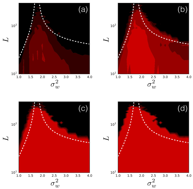
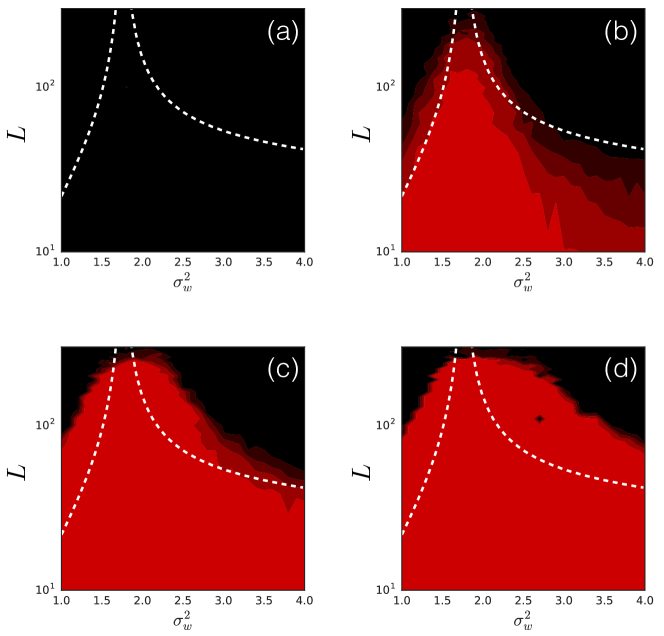
Refer to caption
Figure 7: Training accuracy on MNIST after (a) 45 (b) 304 (c) 2048 and (d) 13780 steps of SGD with learning rate 103superscript10310^{-3}.
Refer to caption
Figure 8: Training accuracy on MNIST after (a) 45 (b) 304 (c) 2048 and (d) 13780 steps of RMSProp with learning rate 105superscript10510^{-5}.