Bayesian and Variational Bayesian approaches for flows in heterogenous random media

Abstract

In this paper, we study porous media flows in heterogeneous stochastic media. We propose an efficient forward simulation technique that is tailored for variational Bayesian inversion. As a starting point, the proposed forward simulation technique decomposes the solution into the sum of separable functions (with respect to randomness and the space), where each term is calculated based on a variational approach. This is similar to Proper Generalized Decomposition (PGD). Next, we apply a multiscale technique to solve for each term (as in [1]) and, further, decompose the random function into 1D fields. As a result, our proposed method provides an approximation hierarchy for the solution as we increase the number of terms in the expansion and, also, increase the spatial resolution of each term. We use the hierarchical solution distributions in a variational Bayesian approximation to perform uncertainty quantification in the inverse problem. We conduct a detailed numerical study to explore the performance of the proposed uncertainty quantification technique and show the theoretical posterior concentration.

1 Introduction

In a physical system governed by differential equations, studying the uncertainty of the underlying system is of great interest. Given the observation from the system (possibly contaminated with errors) inferencing on the underlying parameter and its uncertainty constitutes the uncertainty quantification of the inverse problem [2, 3, 4]. Bayesian methodology provides a natural framework for such problems, through specification of a prior distribution on the underlying parameter and the known likelihood function [5, 6, 7, 8]. The Bayesian inference uses Markov chain Monte Carlo (MCMC) or related methodologies. For MCMC, at each sampling step, for each proposed value of the parameter, we need to solve the underlying equation i.e., the forward problem. The forward solution may not be closed form and we need to apply a numerical technique such as finite element or finite difference methods for that purpose, which can be computationally expensive. The objective of this paper is to combine an efficient forward solution technique with an uncertainty quantification technique in an inverse problem. For that purpose, we use a separation of variable based model reduction technique in combination with a variational Bayesian approach for the inverse problem.

Our current development lies at the interface of forward and inverse problems. Estimating subsurface properties plays an important role in many porous media applications, such as reservoir characterization, groundwater modeling, vadose zone characterization, and so on. In this paper, we consider a model problem of reconstructing permeability field $\kappa(x)$ in the following single-phase flow equation

$$-\nabla\cdot(\kappa(x,\mu)\nabla u(x,\mu)) =f\textrm{ in }\Omega_{x},$$

$$u|_{\partial\Omega_{x}} =0,$$ (1)

for given observations $y$ on pressure field $u$, where $\mu$ is the parameters associated with the permeability field $\kappa$, and $f$ is the known force term.

Uncertainty quantification in an inverse problem can be a daunting task, particularly, for multiscale problems due to scale disparity. These problems require efficient forward simulation techniques that can reduce the degrees of freedom in a systematic way.

The first step in the estimation involves a parameterization of the media properties using some prior information. Typical approaches include Karhunen-Loève type expansion (KLE), where the underlying random field is assumed to be Gaussian. More complex parameterization involves channelized fields [9, 10]. These prior distributions can contain additional random parameters, which require additional prior information and may involve techniques like reversible jump MCMC [9].

For a forward solution technique used in a stochastic inversion, we explore approaches that are based on separation of variables, where we separate uncertainties and the spatial variables. These separation approaches differ from Monte Carlo methods. They allow a fast computation of the solution space over the entire parameter range at a cost of computing each term in the separable expansion. In many cases, these separable expansions converge very fast and requires only a few terms. In our approaches, the solution is sought as a linear combination of separable functions (see e.g., [11, 12, 13] and applications to inverse problems in [14, 15]).

In this paper, we consider an approach proposed in [16] with an overarching goal to do Bayesian inversion. We show that these approaches based on separation of variables can be effectively used within a variational Bayesian framework and, in return, variational Bayesian approaches provide an effective framework for applying separable solution approximation in inverse problems.

Variational Bayesian techniques [17] offer an efficient method of posterior computation, where we approximate the posterior distribution by a closed form recursive estimate, without going into MCMC simulation. Variational Bayesian methods provide fast deterministic posterior computation and can be helpful for uncertainty quantification in inverse problem (cf., [18, 19]). In variational Bayesian methods, we assume that the conditional posterior of different parts of the parameter are independent. To estimate each such part, the full separability assumption , i.e., the separability of the parametric and spatial part and separation of the parametric part over dimension is necessary. Therefore, the full separability gives us a natural framework for a variational algorithm.

For the prior distribution, we use KLE to parametrize the log permeability field assuming Gaussian distribution. For coefficients representing the separable solution form, we also use Gaussian process priors.

Further, we decompose the posterior solution into conditional independent parts and derive a more efficient variational solution. We show the posterior consistency of the proposed method that is the estimated value of the spatial field should be close to the true field under some appropriate metric if some conditions hold. We also show that the forward solution converges to the true solution.

We summarize the main contributions of this work as: 1) Proposing a fully separable representation for forward and inverse problem for the flow equation (1); 2) Proposing a fast UQ technique based on the separable representation; 3) Proposing a novel variational method, based on full separability and achieving further computational efficiency; and 4) Showing the convergence of both the forward solution and the posterior distribution under the proposed method.

In the next section, we provide a detailed description of the model and data generating mechanism and a brief outline of the paper. First, we solve the forward problem under full separability and then, based on the forward solution, we proceed to the inverse problem and uncertainty quantification.

2 Outline of the paper

We consider the flow equation (1). If $\kappa$ is given, solving $u$ is called a forward problem. Given $u$, finding corresponding $\kappa$ constitutes the corresponding inverse problem. Given observed data $y$, we would like to estimate the underlying field $\kappa$. Here, $y$ is the quantity associated with (1) such as fractional flow or pressure data. We further assume an error $\epsilon_{f}$ in the observation in the following form,

$$y =F(\kappa)+\epsilon_{f},$$

$$\epsilon_{f} \sim{{\mathcal{N}}}(0,\sigma^{2}_{f}).$$ (2)

Let $\pi(\kappa)$ be the prior on $\kappa$ and the posterior $\Pi$ is therefore

$$\Pi(\kappa|y)\propto\underbrace{p(y|\kappa)}_{\text{Likelihood}}\underbrace{\pi(\kappa)}_{\text{Prior}}.$$ (3)

The likelihood computation part in each iteration involves a forward solve and therefore can be computationally expensive. The following separable representation can allow a fast likelihood computation.

Separating the spatial and parametric part, we can write, $u=\sum^{N_{1}}_{i=1}a_{i}(\mu)v_{i}(x)$, where $a_{i}(\mu)$ depends on the parametric part of $\kappa$, and $v_{i}(x)$ depends on the spatial variable ([16]). If $\kappa$ is parameterized by finite dimensional $\mu=\{\theta_{1},\dots,\theta_{N_{2}}\}$, we impose another separability condition $a_{i}(\mu)=\prod_{j=1}^{N_{2}}a_{i,j}(\theta_{j})$. With this complete separable representation, we can avoid estimating $a_{i}(\mu)$ in higher dimension and instead estimate low dimensional function $a_{i,j}$. Hence, we have the following fully separable approximation of $u$,

$$\tilde{u}=\sum^{N_{1}}_{i=1}\left(\prod^{N_{2}}_{j=1}a_{i,j}(\theta_{j})\right)v_{i}(x).$$ (4)

Under (4), the solution of $u$ can be expressed as a function depending on parameter $\mu\in\Omega_{\mu}$. To solve the inverse problem and quantify the uncertainty, we explicitly solve the $a_{i,j}$’s over a grid of $\theta_{j}$’s and using a Gaussian process prior on the $a_{i,j}$s, the posterior distribution of $\theta_{j}$’s can be computed. For the parametrization of $\kappa$, we use KL expansion with $N_{2}$ terms, which we discuss later. Before describing the priors and the complete hierarchical model for the inverse problem, the solution for $a_{i,j}$’s for the forward problem is given in the next section.

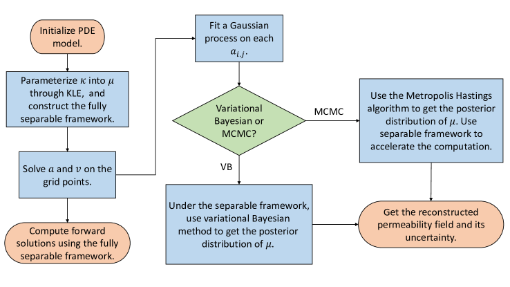
In Section 3, we present a forward solution approach. In Section 4, we write down the priors and hierarchical models for the inverse problem. In Section 5, we describe the MCMC and variational steps explicitly. Later, we introduce the notion of the consistency in Section 6. In Section 7, we conduct numerical studies. We present a simple flowchart in Figure 1 to help understanding the outline of the paper.

Figure 1: A simple flowchart showing the outline of the paper.

3 Forward Solution in Separable Method

For PDE model (1) under the boundary condition a solution can be achieved by solving the variational form,

$$u=\operatorname*{arg\,min}_{u^{*}}\int_{\Omega_{\mu}}\int_{\Omega_{x}}(\frac{1}{2}\kappa|{\nabla}u^{*}|^{2}-fv)dxd\mu.$$

Using this form, we can solve for $a_{i}$ and $v_{i}$ numerically over a grid in $\Omega_{\mu}$. When the dimension of $\Omega_{\mu}$ is bigger then number of required grid over the product space increases exponentially.

To tackle this problem, we further separate the parametric coefficient part as a product of coefficient functions for each individual parameter. Next, we formulate the fully separable method. Inspired by the idea of Proper Generalized Decomposition, we can introduce following approximation of $u$ in (4). Let $a=\{a_{i,j}(\cdot)\},\ v=\{v_{i}(\cdot)\}$, now we try to solve $a$ and $v$ under the variational form.

3.1 Solving $a$ and $v$

For derivation of $a_{i,j}$ and $v_{i}$, let us consider the first term, which contains $a_{1,j}$ and $v_{1}$. Using pure greedy optimization, we want to find $a_{1,j}$ and $v_{1}$ that satisfy

$$(a_{1,j},v_{1})=\operatorname*{arg\,min}_{a_{i,j},v_{1}}\int_{\Omega_{x}}\int_{\Omega_{\mu}}\left(\frac{1}{2}\kappa\left|\nabla\prod^{N_{2}}_{j=1}a_{1,j}v_{1}\right|^{2}-f\prod^{N_{2}}_{j=1}a_{1,j}v_{1}\right)d\mu dx.$$

Set $a_{1}=\prod^{N_{2}}_{j=1}a_{1,j}$. Then, $v_{1}$ solves the following equation

$$-\nabla\cdot\left(\int_{\Omega_{\mu}}\kappa\prod^{N_{2}}_{j=1}a_{1,j}^{2}d\mu\ \nabla v_{1}\right)dx=\int_{\Omega_{\mu}}f\prod^{N_{2}}_{j=1}a_{1,j}\ d\mu.$$ (5)

Similarly, for $a_{1,j}$, we have:

$$a_{1,j}=\frac{\int_{\Omega_{x}}\int_{\Omega_{\mu}\setminus\Omega_{j}}f\prod_{k\neq j}a_{1,k}v_{1}d\mu^{\prime}dx}{\int_{\Omega_{x}}\int_{\Omega_{\mu}\setminus\Omega_{j}}\kappa\prod_{k\neq j}a_{1,k}^{2}d\mu^{\prime}\ |\nabla v_{1}|^{2}dx},$$ (6)

where $\theta_{j}\in\Omega_{j},\ \Omega_{\mu}=\Omega_{1}\bigoplus\Omega_{2}\bigoplus\cdots\bigoplus\Omega_{N_{2}}$ and $\mu^{\prime}\in\Omega_{\mu}\setminus\Omega_{j}.$ In the previous derivation, we notice that we need to calculate the integration on $\Omega_{\mu}$. Although $\Omega_{\mu}$ itself is a high dimensional space, we could compute the integration simply by separating it into $N_{2}$ subspaces:

$$\int_{\Omega_{\mu}}\kappa\prod^{N_{2}}_{j=1}a_{1,j}^{2}d\mu =p\int_{\Omega_{1}}\cdots\int_{\Omega_{N_{2}}}e^{\sum^{N_{2}}_{j}\theta_{j}\phi_{j}}\prod^{N_{2}}_{j=1}a_{1,j}^{2}d\theta_{1}\cdots d\theta_{N_{2}}$$

$$=\prod^{N_{2}}_{j=1}\int_{\Omega_{j}}e^{\theta_{j}\phi_{j}}a^{2}_{1,j}d\theta_{j}$$

and

$$\int_{\Omega_{\mu}\setminus\Omega_{j}}\kappa\prod_{k\neq j}a_{1,k}^{2}d\mu^{\prime}=\prod_{k\neq j}\int_{\Omega_{k}}e^{\theta_{k}\phi_{k}}a^{2}_{1,k}d\theta_{k}.$$

Here, we use $\kappa=e^{\sum_{j=1}^{N_{2}}\theta_{j}\phi_{j}}$, the form we have for KLE parametrization. We discuss the parametrization in details in next section.

Once $a_{1,j}$ and $v_{1}$ are computed, we update $f$ by

$$f_{1}=f+\nabla\cdot(\kappa\nabla\prod^{N_{2}}_{j=1}a_{1,j}v_{1}).$$

We state the whole iteration in Algorithm 1.

Algorithm 1 Find $a_{i,j}$ and $v_{i}$.

1:for $i=1,2,\ldots,N_{1}$ do

2:     $a_{i,j}=1,v_{i}=1.$

3:     $\delta a_{i}=1,\delta v_{i}=1.$

4:     while $\delta a_{i}>tol_{a}$ and $\delta v_{i}>tol_{v}$ do

5:         Let $a^{\prime}_{i,j}=a_{i,j},v^{\prime}_{i}=v_{i}.$

6:         Solve equation (5) for $v_{i}$.

7:         for $j=1,2,\ldots,N_{2}$ do

8:              Using equation (6) to update $a_{i,j}$

9:         end for

10:         Update $\delta v_{i}=||v_{i}-v^{\prime}_{i}||^{2}_{2}$ and $\delta a_{i}=\sum_{j}||a_{i,j}-a^{\prime}_{i,j}||^{2}$

11:     end while

12:     Update $f=f+\nabla\cdot(\kappa\nabla\prod^{N_{2}}_{j=1}a_{i,j}v_{i})$

13:     if $\|f\|<tol_{f}$ then

14:         Stop for loop.

15:     end if

16:end for

3.2 GMsFEM framework for forward problem

In our calculations, we need to solve the PDE for different permeability fields multiple times. For this reason, we use the GMsFEM to reduce computational cost. We use the offline-online procedure to construct GMsFEM coarse spaces. In the offline stage, we first generate the snapshot spaces based on different parameters, then get a low dimensional offline space via model reduction. In the online stage, we use the previous offline basis function to solve a coarse-grid problem for given $\kappa$. For details, we refer to [1, 16, 20, 21, 22]. Note that the GMsFEM becomes particularly important when there are multiple scales and the problem can be reduced over each coarse block.

4 Priors and the inverse problem formulation

Given observations on $y$, to estimate and to quantify the uncertainty of $\kappa$ parameterized by $\mu=\{\theta_{1},\dots,\theta_{N_{2}}\}$, we specify the priors and the steps of MCMC. We can solve $a_{i,j}$ ’s over a grid of points and to capture the approximate nature of the representation (4), we fit a Gaussian process over different values of $\mu$. Under the separation of $a_{i}$’s over $\theta_{i}$’s which results to a product of Gaussian processes.

4.1 Fitting a Gaussian Process on function $a_{i,j}$

Suppose we want to estimate the value of $a_{i,j}$ based on $n_{grid}$ current grid points. For the function $a_{i,j}(\theta_{j})$, from the numerical solution we have the function value $z^{(j)}=(z^{(j)}_{1},z^{(j)}_{2},\cdots,z^{(j)}_{n_{grid}})$ on $\alpha=(\alpha_{1},\alpha_{2},\cdots,\alpha_{n_{grid}})$ which are the grids of $\theta_{j}$. We assume $z_{i}$ are observed with Gaussian white noise ${\mathcal{N}}(0,\sigma_{1}^{2})$. We set the covariance matrix $K$ using squared exponential covariance:

$$K(\alpha^{*},\alpha^{**})=\sigma_{a}^{2}\exp\left[-\frac{1}{2}\left(\frac{\alpha^{*}-\alpha^{**}}{\lambda}\right)^{2}\right]$$

and

$$a_{i,j}(\cdot)\sim\mathscr{GP}(0,K),$$ (7)

where $\lambda$ is the length scale and $\sigma_{a}$ is the variance. Then, for a new single input $\alpha_{*}$, define $\mu_{*}$ as the mean estimation of $a_{i,j}(\alpha_{*})$, and $\sigma_{*}^{2}$ as the variance estimation of $a_{i,j}(\alpha_{*})$, we have $a_{i,j}(\alpha_{*})\sim\mathcal{N}(\mu_{*},\sigma_{*})$ and

$$\mu_{*} =K_{*n_{grid}}(K_{n_{grid}}+\sigma_{1}^{2}I)^{-1}z^{(j)}$$

$$\sigma_{*}^{2} =K_{*}-K_{*n_{grid}}p(K_{n_{grid}}+\sigma_{1}^{2}I)^{-1}K_{*n_{grid}}^{\top}+\sigma_{1}^{2},$$ (8)

where $K_{*n_{grid}}$ is the covariance vector between $\alpha_{*}$ and $(\alpha_{1},\alpha_{2},\cdots,\alpha_{n_{grid}})$, $K_{n_{grid}}$ is the covariance matrix of vector $(\alpha_{1},\alpha_{2},\cdots,\alpha_{n_{grid}})$, and $K_{*}=\sigma_{a}^{2}$. The computational cost for each input point is $\mathcal{O}(N)$ for mean and $\mathcal{O}(N^{3})$ for the variance, with $N=n_{grid}$.

4.2 Permeability parametrization

To obtain a permeability field in terms of an optimal $L^{2}$ basis, we use the KLE. Considering the random field $\mathscr{Y}({x},\tilde{\omega})=\log[k({x},\tilde{\omega})]$, where $\tilde{\omega}$ represents randomness. We assume a zero mean $E[\mathscr{Y}({x},\tilde{\omega})]=0$, with a known covariance operator $R({x},{y})=E\left[\mathscr{Y}({x})\mathscr{Y}({y})\right]$. Then, $\mathscr{Y}(x,\tilde{\omega})$ has following Reproducing Kernel Hilbert Space (RKHS) representation

$$\mathscr{Y}({x},\tilde{\omega})=\sum_{k=1}^{\infty}\mathscr{Y}_{k}(\tilde{\omega})\Phi_{k}({x}),\qquad$$

with

$$\mathscr{Y}_{k}(\tilde{\omega})=\int_{\Omega}\mathscr{Y}(x,\tilde{\omega})\Phi_{k}(x)dx.$$

The functions $\{\Phi_{k}(x)\}$ are eigenvectors of the covariance operator $R(x,y)$, and form a complete orthonormal basis in $L^{2}(\Omega)$,that is

$$\int_{\Omega}R({x},{y})\Phi_{k}({y})d{y}=\lambda_{k}\Phi_{k}({x}),\qquad k=1,2,\ldots,$$ (9)

where $\lambda_{k}=E[\mathscr{Y}_{k}^{2}]>0$, $E[\mathscr{Y}_{i}\mathscr{Y}_{j}]=0$ for all $i\neq j$. Let $\theta_{k}=\mathscr{Y}_{k}/\sqrt{\lambda_{k}}$. Hence, $E[\theta_{k}]=0$ and $E[\theta_{i}\theta_{j}]=\delta_{ij}$ and we have

$$\mathscr{Y}({x},\tilde{\omega})=\sum_{k=1}^{\infty}\sqrt{\lambda_{k}}\theta_{k}(\tilde{\omega})\Phi_{k}({x}),$$ (10)

where $\Phi_{k}$ and $\lambda_{k}$ satisfy (9). We truncate the KLE (10) to a finite number of terms and keep the leading-order terms (quantified by the magnitude of $\lambda_{k}$), and capture most of the energy of the stochastic process $\mathscr{Y}(x,\tilde{\omega})$. For an $N$-term KLE approximation

$$\mathscr{Y}^{N}=\sum_{k=1}^{N}\sqrt{\lambda_{k}}\theta_{k}\Phi_{k},$$

the energy ratio of the approximation is defined by

$$e(N):=\frac{E\|\mathscr{Y}^{N}\|^{2}}{E\|\mathscr{Y}\|^{2}}=\frac{\sum_{k=1}^{N}\lambda_{k}}{\sum_{k=1}^{\infty}\lambda_{k}}.$$

If the eigenvalues $\{\lambda_{k}\}$ decay very fast, then the truncated KLE with the first few terms would be a good approximation of the stochastic process $\mathscr{Y}(x,\omega)$ in the $L^{2}$ sense. In our simulations, we use the prior $\theta_{k}\sim{\mathcal{N}}(0,1)$.

4.3 Hierarchical Model

From the likelihood equation (2) and the priors in (10) and (7), the full hierarchical model can be written. Writing $\tilde{u}=\sum^{N_{1}}_{i=1}\left(\prod^{N_{2}}_{j=1}a_{i,j}(\theta_{j})\right)v_{i}(x)$, as in the fully separable representation given in (4), we have

$$y =F(\kappa)+\epsilon_{f},$$

$$\epsilon_{f} \sim{\mathcal{N}}(0,\sigma^{2}_{f}),$$

$$a_{i,j}(\cdot) \sim\mathscr{GP}(0,K),$$

$$log(\kappa({x},\tilde{\omega})) =\sum_{k=1}^{\infty}\sqrt{\lambda_{k}}\theta_{k}(\tilde{\omega})\Phi_{k}({x}),$$

$$\theta_{k} \sim{\mathcal{N}}(0,1).$$ (11)

5 Posterior Calculation

Suppose we have $M$ observations $y_{1},y_{2},\cdots,y_{M}\in R$ of $u$ at the locations $x_{1},x_{2},\cdots,x_{M}\in\Omega_{x}$. Then, we define vector $V_{i}=\left(v_{i}(x_{1}),v_{i}(x_{2}),\cdots,v_{i}(x_{M})\right)^{\intercal}$, where $v_{i}$ is the solution of (5), and let $y=(y_{1},y_{2},\cdots,y_{M})^{\intercal}$. We also assume that each observation contains Gaussian white noise ${\mathcal{N}}(0,\sigma_{y}^{2})$. Based on the separated method and Bayes framework the posterior is given by:

$$\Pi(\mu,a|y)\varpropto p(y|a)\cdot\pi(a|\mu)\cdot\pi(\mu).$$ (12)

5.1 Variational Bayesian Method

We present a brief overview of the variational Bayesian method. For the observation $Y$, parameter ${\bf\Theta}$ and prior $\Pi({\bf\Theta})$ on it, let the joint distribution and posterior be ${p(Y,\Theta)}$ and ${\Pi({\bf\Theta}|Y)}$, respectively. Then

$$\log p(Y)=\int\log\frac{p(Y,\Theta)}{q({\bf\Theta})}q({\bf\Theta})d({\bf\Theta})+KL(q({\bf\Theta}),\Pi({\bf\Theta}|Y)),$$

for any density $q({\bf\Theta})$. Here $KL(p,q)=E_{p}(\log\frac{p}{q})$, the Kullback-Leibler distance between $p$ and $q$. Thus,

$$KL(Q({\bf\Theta}),p(Y,{\bf\Theta}))=KL(Q({\bf\Theta}),\Pi({\bf\Theta}|Y))-\log p(Y).$$ (13)

Given $Y$, we minimize $KL(Q({\bf\Theta}),p(Y,{\bf\Theta}))$ under separability. Minimization of the L.H.S of (13) analytically may not be possible in general and therefore, to simplify the problem, it is assumed that the parts of ${\bf\Theta}$ are conditionally independent given $Y$. That is

$$Q({\bf\Theta})=\prod_{i=1}^{s}q(\eta_{i})$$

and $\cup_{i=1}^{s}\eta_{i}={\bf\Theta}$ is a partition of the set of parameters ${\bf\Theta}$. Minimizing under the separability assumption, an approximation of the posterior distribution is computed. Under this assumption of minimizing L.H.S of (13) with respect to $q(\eta_{i})$, and keeping the other $q(\eta_{j}),j\neq i$ fixed, we develop the following mean field approximation equation:

$$q(\eta_{i})\propto\exp(E_{-i}\log(p(Y,{\bf\Theta})),$$ (14)

where the subscript $E_{-i}$ stands for expectation with respect to variables other than those included in $\eta_{i}$. The variational solution is exact and converges to the KL minimizer in the proposed class rapidly.

Finally for our case, the posterior distribution of parameter $\mu$ and $a$ given observations $y$ is approximated by a variational distribution:

$$P(\mu,a|y)=Q(\mu,a).$$

For a fixed index $j$, $\theta_{j}$ and $a_{i,j}$ can be highly correlated due to Gaussian process fitting. We have the following from equation (8)

$$E(a_{i,j}) =K_{\theta_{j}n}(K_{n}+\sigma_{1}^{2}I)^{-1}z^{(j)}$$

$$Var(a_{i,j}) =K_{\theta_{j}}-K_{{}_{\theta_{j}}n}(K_{n}+\sigma_{1}^{2}I)^{-1}K_{\theta_{j}n}^{\intercal}+\sigma_{1}^{2}.$$

We group these variables based on index $j$:

$$\mathcal{G}_{j}=\{\theta_{j},a_{1,j},a_{2,j},\cdots,a_{N_{1},j}\}\text{ for }j=1,2,\cdots,N_{2}$$

and then we factorize the variational distribution into these groups,

$$Q(\mu,a)=\prod_{j=1}^{N_{2}}q(\theta_{j},a_{1,j},\cdots,a_{N_{1},j}).$$ (15)

Minimizing the Kullback-Leibler divergence of $P$ from $Q$, the best approximation of each $q_{j}$ is

$$\ln q(\mathcal{G}_{j})=E_{\theta_{k},a_{i,k},k\neq j}\left[\ln P(\mu,a,y)\right]+\text{constant}.$$ (16)

In the following part we write $E_{\theta_{k},a_{i,k},k\neq j}$ as $E_{-j}$ in abbreviation.

Next, our goal is to give a complete form of Equation (16). For this, we suppose we have $M$ observations $y_{1},y_{2},\cdots,y_{M}\in R$ on $x_{1},x_{2},\cdots,x_{M}\in\Omega_{x}$, then we shrink $v_{i}(x)$ into an $M$ dimension vector

$$V_{i}=\left(v_{i}(x_{1}),v_{i}(x_{2}),\cdots,v_{i}(x_{M})\right)^{\intercal}$$

and let $y=(y_{1},y_{2},\cdots,y_{M})^{\intercal}$. We also assume that each observation contains Gaussian white noise ${\mathcal{N}}(0,\sigma_{y}^{2})$.

Furthermore, we use Gaussian distribution as prior distribution for $\theta_{j}$,

$$\theta_{j}\sim{\mathcal{N}}(\theta_{0},\sigma_{0}^{2}).$$

Then, we have

$$\ln q(\mathcal{G}_{k})={} E_{-k}\left[\ln P(\mu,a,y)\right]+\text{constant}$$

$$={} E_{-k}\left[\ln P(y|a)+\ln P(a|\mu)+\ln P(\mu)\right]+\text{constant}$$

$$={} E_{-k}\left[-\frac{\left\lVert y-\sum^{N_{1}}_{i=1}\left(\prod^{N_{2}}_{j=1}a_{i,j}\right)V_{i}\right\rVert_{2}^{2}}{2\sigma_{y}^{2}}\right]$$

$$+E_{-k}\left[\sum_{i=1}^{N_{1}}\sum_{j=1}^{N_{2}}\ln\frac{\exp\left(-\frac{1}{2\sigma_{i,j}^{2}(\theta_{j})}|a_{i,j}-\mu_{i,j}(\theta_{j})|^{2}\right)}{\sqrt{2\pi}\sigma_{i,j}(\theta_{j})}\right]$$

$$+E_{-k}\left[\sum_{j=1}^{N_{2}}\ln\frac{\exp\left(-\frac{1}{2\sigma_{0}^{2}}(\theta_{j}-\theta_{0})^{2}\right)}{\sqrt{2\pi}\sigma_{0}}\right]+C.$$

Define $R_{i}=\prod_{j\neq k}{a_{i,j}}$ and re-write the above equality as

$$\ln q(\mathcal{G}_{k})={} E_{-k}\left[-\frac{1}{2\sigma_{y}^{2}}\left\lVert y-\sum^{N_{1}}_{i=1}a_{i,k}R_{i}V_{i}\right\rVert_{2}^{2}\right]$$

$$-\sum_{i=1}^{N_{1}}\frac{1}{2\sigma_{i,k}^{2}(\theta_{k})}|a_{i,k}-\mu_{i,k}(\theta_{k})|^{2}-\ln\prod_{i=1}^{N_{1}}\sigma_{i,k}(\theta_{k})$$

$$-\frac{1}{2\sigma_{0}^{2}}(\theta_{k}-\theta_{0})^{2}+C.$$

We need to calculate the marginal distribution of $\theta_{j}$. Let $A_{k}=(a_{1,k},\cdots,a_{N_{1},k})^{\intercal}\in\mathbb{R}^{N_{1}}$. Then

$$q(\theta_{k}) =\int_{R^{N_{1}}}\ q(\theta_{k},A_{k})\ dA_{k}$$

$$=\int_{R^{N_{1}}}e^{-A_{k}^{\intercal}\Sigma(\theta_{k})A_{k}+\beta^{\intercal}(\theta_{j})A_{k}}\ dA_{k}\cdot\frac{1}{\prod_{i}\sigma_{i,k}(\theta_{k})}\cdot e^{-\sum_{i=1}^{N_{1}}\frac{\mu_{i,k}^{2}(\theta_{k})}{2\sigma_{i,k}^{2}(\theta_{k})}-\frac{(\theta_{k}-\theta_{0})^{2}}{2\sigma^{2}_{0}}}\cdot C,$$

where

$$\Sigma_{m,m}(\theta_{k}) =\frac{1}{2\sigma^{2}_{y}}E(R_{m}^{2})V_{m}^{\intercal}V_{m}+\frac{1}{2\sigma_{m,k}^{2}(\theta_{k})}\quad\text{for}\quad m=1,2,\cdots,N_{1},$$

$$\Sigma_{m,n}(\theta_{k}) =\frac{1}{2\sigma^{2}_{y}}E(R_{m}R_{n})V_{m}^{\intercal}V_{n}\quad\text{for}\quad m\neq n,$$

$$\beta_{m}(\theta_{k}) =\frac{1}{\sigma_{y}^{2}}E(R_{m})V_{m}^{\intercal}y+\frac{\mu_{m,k}(\theta_{k})}{\sigma_{m,k}^{2}(\theta_{k})}\quad\text{for}\quad m=1,2,\cdots,N_{1}.$$

Note that

$$\int_{R^{N_{1}}}e^{-A_{k}^{\intercal}\Sigma A_{k}+\beta^{\intercal}A_{k}}\ dA_{k}=\sqrt{\frac{\pi^{N_{1}}}{\det\Sigma}}\exp(\frac{1}{4}\beta^{\intercal}\Sigma^{-1}\beta).$$

Therefore,

$$q(\theta_{k})\propto q^{*}(\theta_{k})=\frac{1}{\sqrt{\det\Sigma}\cdot\prod_{i}\sigma_{i,k}(\theta_{k})}\exp\left(\frac{1}{4}\beta^{\intercal}\Sigma^{-1}\beta-\frac{1}{2\sigma_{0}^{2}}(\theta_{k}-\theta_{0})^{2}-\sum_{i=1}^{N_{1}}\frac{\mu_{i,k}^{2}(\theta_{k})}{2\sigma_{i,k}^{2}(\theta_{k})}\right).$$ (17)

We can compute the joint for $\theta_{k},a_{p,k}$,

$$q^{*}(\theta_{k},a_{p,k})=\frac{1}{\sqrt{\det\Sigma}\cdot\prod_{i}\sigma_{i,k}(\theta_{k})}\\ e^{\left(\frac{1}{4}\beta^{\intercal}\Sigma^{-1}\beta-c_{p}(\theta_{k})-\frac{(\theta_{k}-\theta_{0})^{2}}{2\sigma^{2}_{0}}-\frac{1}{2\sigma_{y}^{2}}\left(a_{p,k}^{2}E(R_{p}^{2})v_{p}^{\intercal}v_{p}\right)\right)},$$ (18)

where

$$\Sigma_{m,m} =\frac{1}{2\sigma^{2}_{y}}E(R_{m}^{2})V_{m}^{\intercal}V_{m}+\frac{1}{2\sigma_{m,k}^{2}(\theta_{k})}\quad\text{for}\quad m\neq p,$$

$$\Sigma_{m,n} =\frac{1}{2\sigma^{2}_{y}}E(R_{m}R_{n})V_{m}^{\intercal}V_{n}\quad\text{for}\quad m\neq n,m\neq p,n\neq p,$$

$$\beta_{m} =p\frac{1}{\sigma_{y}^{2}}E(R_{m})V_{m}^{\intercal}y+\frac{\mu_{m,k}(\theta_{k})}{\sigma_{m,k}^{2}(\theta_{k})}+\frac{1}{\sigma_{y}^{2}}a_{p,k}E(R_{p}R_{m})V_{p}^{\intercal}V_{m},$$

$$c_{p}(\theta_{k}) =\sum_{i=1}^{N_{1}}\frac{\mu_{i,k}^{2}(\theta_{k})}{2\sigma_{i,k}^{2}(\theta_{k})}+\frac{(a_{p,k}-\mu_{p,k})^{2}}{2\sigma_{p,k}^{2}(\theta_{k})}-\frac{1}{\sigma_{y}^{2}}a_{p,k}E(R_{p})v_{p}^{\intercal}y.$$

The details of the expansions are given in Appendix A1. Next, we write down the algorithm for Variational Bayesian method in Algorithm 2.

Algorithm 2 Variational Bayesian Method.

1:Set initial value $\theta_{j}=0$ for all $j$.

2:Calculate $E(a_{i,j})$ from (8) for all $i,j$.

3:Calculate $E(R_{m}),\ E(R_{m}^{2})$ and $E(R_{m}R_{n})$ by (30).

4:Set $\delta\theta=1,\delta a=1.$

5:while $\delta a>tol_{a}$ and $\delta\theta>tol_{\theta}$ do

6:     Let $E(a^{\prime})=E(a),E(\theta^{\prime})=E(\theta).$

7:     for $j=1,2,\cdots,N_{2}$ do

8:         Use equations (27) to update $E(\theta_{j})$ and $\sigma_{\theta_{j}}$.

9:         for $i=1,2,\cdots,N_{1}$ do

10:              Use equations (29) to update $E(a_{i,j})$ and $\sigma_{a_{i,j}}$.

11:         end for

12:         Update $E(R_{m}),\ E(R_{m}^{2})$ and $E(R_{m}R_{n})$ by (30).

13:     end for

14:     Update $\delta\theta=\sum_{j}||E(\theta_{j})-E(\theta_{j}^{\prime})||^{2}_{2}$ and $\delta a=\sum_{i,j}||E(a_{i,j})-E(a^{\prime}_{i,j})||^{2}$

15:end while

16:Use equations (28) to get $E(\kappa)$ and $\sigma(\kappa)$.

5.2 MCMC method

From the posterior density given in (12), we use the Metropolis-Hastings Gibbs sampling algorithm from the following set up:

$$p(y|a) \varpropto\exp\left(-\frac{1}{\sigma_{y}^{2}}\left\lVert y-\sum^{N_{1}}_{i=1}\left(\prod^{N_{2}}_{j=1}a_{i,j}\right)V_{i}\right\rVert^{2}\right)$$

$$\pi(a|\mu) \varpropto\prod^{N_{1}}_{i=1}\prod^{N_{2}}_{j=1}\ \exp\left(-\frac{1}{\sigma_{\theta_{j}}^{2}}|a_{i,j}-\mu_{\theta_{j}}|^{2}\right)$$

$$\pi(\mu) \varpropto\prod^{N_{2}}_{j=1}\pi(\theta_{j}),$$

where $y$ are observations, $a=\{a_{i,j}\},\ \mu=(\theta_{1},\cdots,\theta_{N_{2}}),\ \mu_{\theta_{j}}$ and $\sigma_{\theta_{j}}^{2}$ are mean and variance estimation from the Appendix.

6 Some convergence analysis

To show the convergence of the proposed method, we need to show the convergence of the forward and the inverse problems. For the forward problem, we show that the proposed separable representation can adequately approximate $u$. The greedy algorithm for the variational form converges and the solution converges to $u$ in some appropriate metric. For the inverse problem solution, given the observed values, under some conditions, the posterior distribution of $\kappa$ (or $\mu$) converges to the true parameter value in distributional sense.

6.1 Convergence of the forward problem

In Section 3, we introduced fully separated framework for parameter-dependent elliptic partial differential equations and provided an iterative algorithm. Next, we state some convergence results following [13] for this algorithm. We restrict ourselves to the simplest case. Find $a_{i}$ in $L^{2}(\Omega_{\mu})$ and $v_{i}$ in $H^{1}_{0}(\Omega_{x})$ , such that $u=\sum_{i\geq 1}a_{i}(\mu)v_{i}(x)$ is the solution of

$$-\nabla\cdot(\kappa(x,\mu)\nabla u(x,\mu)) =f\textrm{ in }\Omega_{x},$$

$$u|_{\partial\Omega_{x}} =0,$$ (19)

given $0<c_{1}\leq\kappa(x,\mu)\leq c_{2}<\infty$ in the bounded space $\Omega$, where $\mu\in\Omega_{\mu},\ x\in\Omega_{x}$, and $\Omega=\Omega_{\mu}\times\Omega_{x},\ \Omega_{\mu}\in R^{N_{2}},\ \Omega_{x}\in R^{2}$. Following [13], we introduce the tensor product Hilbert space

$$\Gamma(\Omega)=L^{2}(\Omega_{\mu})\bigotimes H^{1}_{0}(\Omega_{x})$$ (20)

with inner product:

$$\langle u,v\rangle=\int_{\Omega}\kappa(x,\mu)\nabla u(x,\mu)\cdot\nabla v(x,\mu)\quad u,v\in\Gamma$$

and the associated norm

$$\|u\|^{2}=\int_{\Omega}\kappa(x,\mu)|\nabla u(x,\mu)|^{2}.$$

Note that

$$(a_{n},v_{n})=\operatorname*{arg\,min}_{(a,v)\in L^{2}(\Omega_{\mu})\times H^{1}_{0}(\Omega_{x})}\int_{\Omega}\frac{1}{2}\kappa|\nabla(a\otimes v)|^{2}-\int_{\Omega}f_{n-1}\cdot(a\otimes v).$$ (21)

Now we introduce $u_{n}$ satisfying

$$-\nabla\cdot(\kappa\nabla u_{n}) =f_{n}\textrm{ in }\Omega_{x},$$

$$u_{n}|_{\partial\Omega_{x}} =0,$$ (22)

then we have

$$u_{n}=u_{n-1}-a_{n}\otimes v_{n}$$ (23)

therefore $u_{n}=u_{0}-\sum^{n}_{i=1}a_{i}\otimes v_{i}$. We denote the tensor product $a\otimes v$ as

$$a\otimes v(\mu,x):=a(\mu)\cdot v(x).$$

Following [13], we can prove the following lemma.

Theorem 1.

Assume that $(a_{n},v_{n})$ satisfies (21). Denote the energy at iteration $n$ as

$$E_{n}=\frac{1}{2}\int_{\Omega}\kappa|\nabla(a_{n}\otimes v_{n})|^{2}-\int_{\Omega}f_{n-1}\ a_{n}\otimes v_{n},$$

then we have

$$\lim_{n\rightarrow\infty}E_{n}=\lim_{n\rightarrow\infty}\|a_{n}\otimes v_{n}\|=0.$$ (24)

Moreover,

$$\lim_{n\rightarrow\infty}u_{n}=0\text{ in }\Gamma,$$ (25)

where $\Gamma$ is defined in (20), and

$$\lim_{n\rightarrow\infty}f_{n}=0\text{ in }\Gamma^{*}.$$ (26)

where $\Gamma^{*}$ is the dual space of $\Gamma$.

Proof.

Given in Appendix A2. ∎

Based on this convergence, one can estimate the difference between the posterior that uses truncated series and the posterior that uses all the terms in appropriate norms and show that this difference is small independent of the dimension of the problem [7, 23, 6].

6.2 Consistency of Bayesian Method

In this section, we discuss and derive the consistency of Bayesian methodology. The main idea is that if we have more and more observations, the posterior distribution will concentrate around true data generating distribution (see e.g., [24]). Even though, we have observations on finitely many grids, posterior consistency is a desirable property for an estimator to have. If the proposed model is true and if we have enough prior mass around the true parameter then the likelihood will pull the posterior distribution around the true parameter value. Here, we assume the data generating model, is given in (2), posterior in (3) and the priors are (7) and (10). We also restrict $\theta_{j}$’s to a compact set. In this setting, we suppose, $f_{\kappa}$ is the density for the $\kappa$ in (2) and $\kappa^{*}$ is the true permeability field. Furthermore, let $f^{*}_{x}(y)$ be the true data generating density at $x\in\Omega_{x}$, where $y\in\Omega_{y}$, a subset of Euclidean space. We assume we have observation in $x_{1},\dots,x_{M}$ under the measure $H(x)$ on $\Omega_{x}$. For a fixed design point, we denote the empirical measure $H_{M}$. Then, we have the following consistency theorem (cf. [24]).

Theorem 2.

For the model and prior setting given in equation (11), for any neighborhood $U_{\epsilon}$ of $f^{*}_{x}(y)$ given as $\int_{\Omega_{x}}\int_{\Omega_{y}}(\sqrt{f_{x}(y)}-\sqrt{f^{*}_{x}(y)})^{2}dydH(x)<\epsilon$, we have $\Pi(U_{\epsilon}|data)\rightarrow 1$ with probability 1 as $M\rightarrow\infty$.

The details are given in Appendix A2. The proof uses our separation argument and additional conditions on the priors. Under the given prior, we have positive probability around any $L_{\infty}$ neighborhood of $a_{i}(\{\theta\})$. This condition ensures positive probability in any Kullback-Leibler neighborhood of $f^{*}$. Then, given the ratio of the likelihood under true density and any other density incerases to infinity exponentially with $M$, the result follows.

If the observations points are fixed design points given by an empirical measure $H_{M}$, then we will have posterior concentration on $U_{\epsilon}$, that is the set given by, $\int_{\Omega_{x}}\int_{\Omega_{y}}(\sqrt{f_{x}(y)}-\sqrt{f^{*}_{x}(y)})^{2}dydH_{M}(x)<\epsilon$. For the convenience, here we assume that the design points are coming from underlying $H$ on $\Omega_{x}$, with density $h(x)$.

7 Numerical Results

In this section, we first apply our fully separated method for the forward problem. Then under the structure of fully separated method, we use MCMC method and Variational Bayesian Method on inverse problem and Uncertainty Quantification.

7.1 Results for Forward Problem

In order to calculate $a_{i,j}$ and $v_{i}$, we first need to define a range on our parameter $\theta_{j}$. Based on our prior information $\theta_{j}\sim{\mathcal{N}}(0,1)$, we simply let $\theta_{j}\in[\theta_{\min},\theta_{\max}]$ and $\theta_{\min}=-5,\ \theta_{\max}=5.$ When $N_{2}\leq 200$, this range will cover more than $99.99\%$ of $\theta$ according to our standard Gaussian prior. We choose $21$ grid points evenly located in interval $[\theta_{\min},\theta_{\max}]$, which are the grid points of our discrete function $a_{i,j}$.

We test our model for $10$ and $30$ KL basis separately. For $N_{2}=10$, we choose $N_{1}=10$. For $N_{2}=30$, we choose $N_{1}=50$. We use fully separated method to get $a$ and $v$, thus given parameters we have $u_{fs}$. The calculation is performed on $50\times 50$ grid. To test the result, we randomly sample $100$ samples of $\mu=(\theta_{1},\cdots,\theta_{N_{2}})$ on grid points based on the prior, then use FEM method to calculate $u_{fem}$ as the accurate result. Finally, we compute relative $L^{2}$ error and relative energy error between $u_{fem}$ and $u_{fs}$,

Error	$N_{2}=10$	$N_{2}=30$
mean relative $L^{2}$ error	0.0260%	0.0840%
mean relative energy error	0.4728%	0.4828%
max relative $L^{2}$ error	0.0882%	0.1942%
max relative energy error	0.7256%	0.8772%

Table 1: Error in forward model.

We can see that all the relative errors are under $1\%$ (see Table 1). Therefore, our fully separated method performs well for the forward problem.

7.2 Results for Inverse Problem

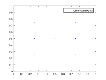
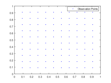
Given $M$ observations of $u$, we would like to estimate and to quantify the uncertainty of $\kappa$ parameterized by $\mu=(\theta_{1},\dots,\theta_{N_{2}})$. Let $y=(y_{1},\cdots,y_{M})$ be observations. We assume the locations of these observations are evenly distributed on $\Omega_{x}$ as Figure 2 shows. The number of observations could be small (9 points) or large (100 points) in our model. Note that on our $50\times 50$ grid, even 100 observation points only contains 4% of total output data, which leads to ill-posedness of the inverse problem. We use Markov Chain Monte Carlo and Variational Bayesian Method separately to reconstruct $\kappa$. We use KL expansion to generate the reference field $\kappa_{ref}$ based on our prior. In this example, we choose isotropic random Gaussian field with correlation function $C(\alpha,\beta)$ given by $C(\alpha,\beta)=\sigma_{gf}^{2}\exp(-\frac{|\alpha-\beta|^{2}}{2l_{0}^{2}})$, where $l_{0}$ is the correlation lengths in both direction and $\sigma_{gf}$ determines the variation of the field. Here we let $\sigma_{gf}=0.2,\ l_{0}=0.1$.

(a) Fewer observations.

(b) More observations.

Figure 2: Locations of fewer and more observation points.

We set our Gaussian process parameters as $\sigma_{a}=1$, $\sigma_{1}=10^{-3}$, $\lambda=1$. We let $\sigma_{y}$ be 1% of the mean observed value. For MCMC, we use $10^{7}$ iterations and $10^{5}$ burn-in. For variational Bayesian Method, we use trapezoidal method to do numerical integration and split the domain into 50 intervals, and assume independence between different $a_{i,j}$ to ease our computational complexity. All our examples are performed by Matlab on a 16-Core CPU.

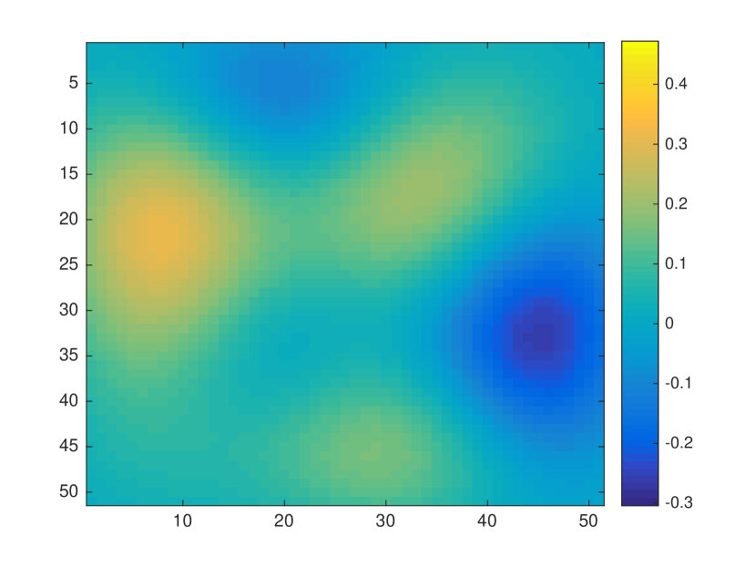
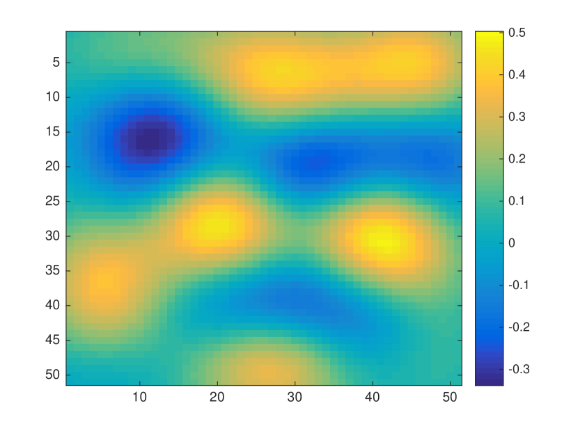
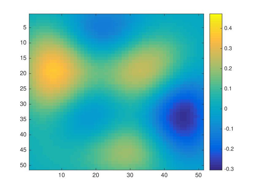
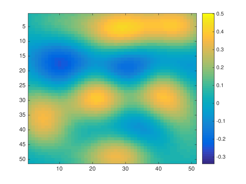
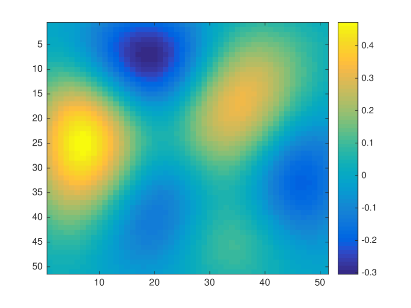
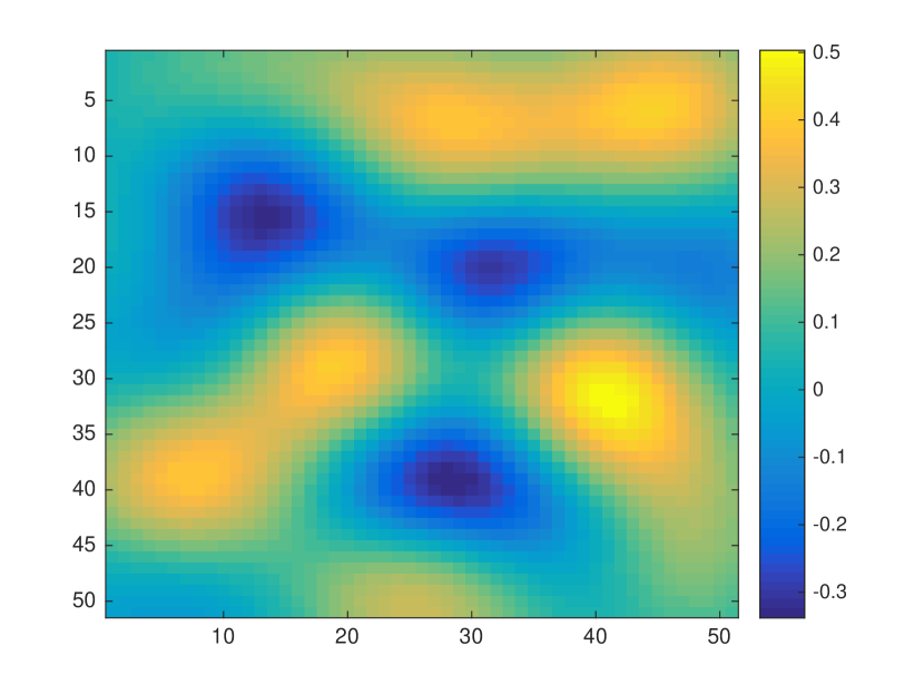
In the case of fewer (9 points, 0.36% of total output) observations, due to the lack of observations, the problem become very ill-posed, which makes it difficult to reconstruct complicated field, thus we use a rather smooth field as reference field. In the case of more (100 points, 4% of total output) observations, we try to reconstruct more complicated field. For the smooth case, we use $(a,v)$ of $N_{2}=10$, and for we use $(a,v)$ of $N_{2}=30$, as in the forward problem example. The result is shown in Figure 3. We can see that both the VB and MCMC methods give good reconstructions on the reference log permeability fields. Due to the lack of observation points in the left column, some details of the field cannot be reconstructed well, while the results in the right column with more observations have shown more details of the reference field. Moreover, from (b), (d) and (f) of Figure 3, it’s clear that the variational Bayesian method gives a smoother and more accurate result over the reconstructed field than the result from MCMC method, thus performs better in this case.

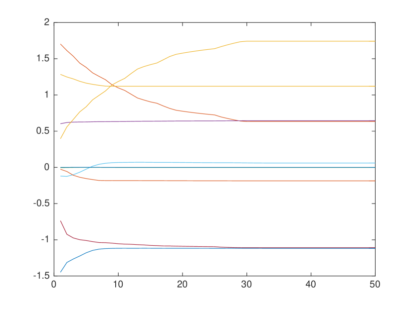
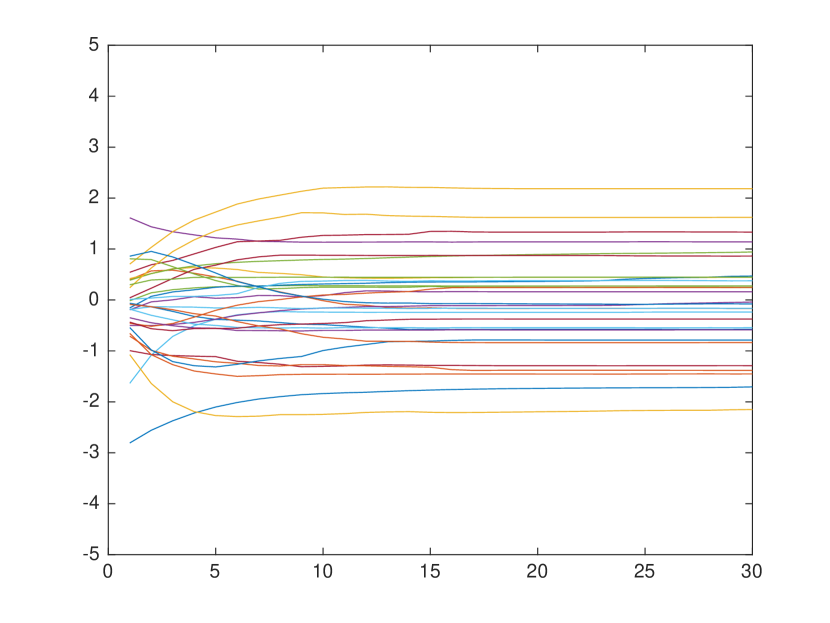
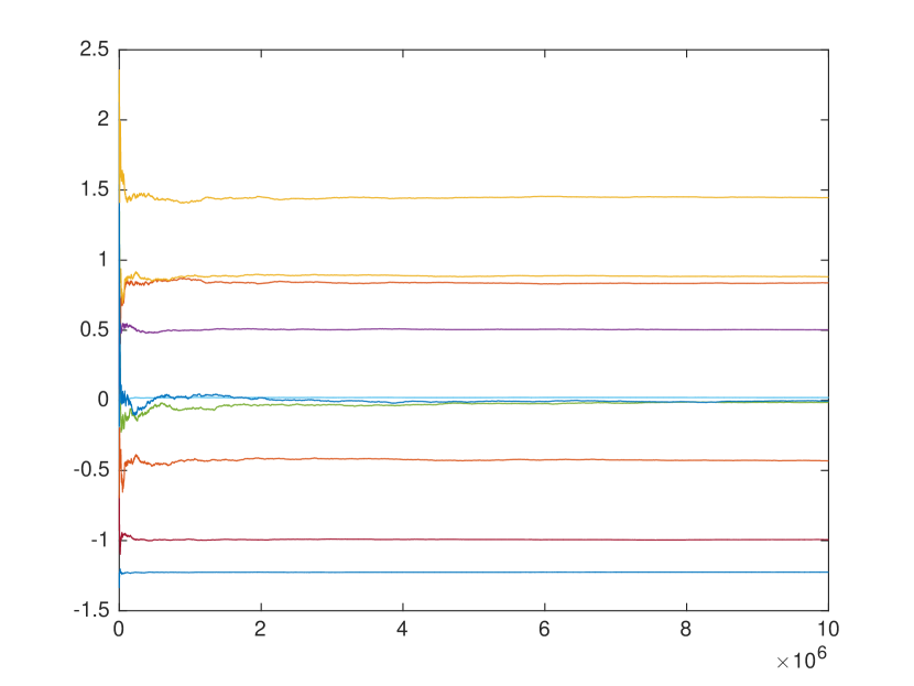
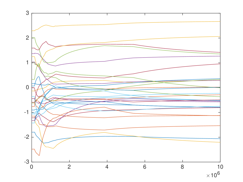
Define $E\mu$ as the posterior mean of $\mu$ in each iteration such that $E\mu=(E\theta_{1},E\theta_{2},\dots,E\theta_{N_{2}})$, we compare the trace of all $E\theta_{j}$ from MCMC and variational Bayesian method in Figure 4 for both fewer and more observations. Variational Bayes converges over a smooth path over first few iterations. With the increase in the dimensions of $\mu$ won’t increase the steps VB method need to converge, while the number of steps that MCMC needs clearly depends largely on the dimensions of $\mu$, which makes variational Bayesian method a preferred choice when dealing with high-dimensional problems. Finally, we show the distributions of parameters in the complicated case as we draw the posterior and prior of first 8 $\theta_{j}$ from KLE in Figure 6.

About the computational cost for variational method, we can use parallel processing for $i=1,2,\cdots,N_{1}$ inside each iterations (line 9 to 11 in Algorithm 2), but for MCMC we could not do parallel processing on a single chain since it is a Markov process. We do a runtime comparison between variational Bayesian method and MCMC method in Table 2. Similarly, we could perform parallel processing in line 8-10 of Algorithm 1 on the fully separated forward problem framework. Moreover, when we use MCMC method, computational time inside each iteration with fully separated framework is much faster than the one without our framework (eg. 0.0025s compare to 0.022s for complicated case here), which makes a significant difference when the number of iterations is very large in most cases.

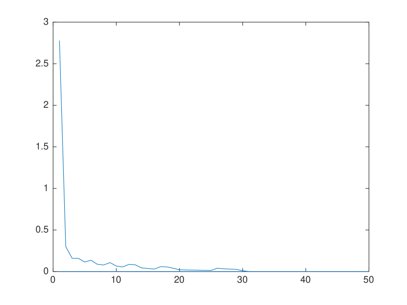
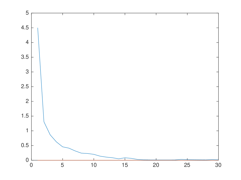
The variational Bayes estimator provides an adequate posterior approximation, while converging very fast, even in complicated cases. We define $\delta\mu$ as the $L^{2}$ norm of the differences of $E\mu$ between adjacent variational Bayesian iterations. A convergence diagnostic can be found in Figure 5, where the fast convergence can be noticed.

8 Discussion

In this paper, we study the uncertainty quantification in inverse problems. We consider a multiscale diffusion problem and use separation of stochastic and spatial variables. A new separation technique is introduced. Under separable representation, proposed Bayesian approaches provide an accurate and fast solution of the inverse problem and provide measure of uncertainty of the parameters given the data. A fast variational Bayes based posterior approximation algorithm has been introduced which produces further computational efficiency and an accurate estimation of the underlying field.

(a) Reference log permeability field (smooth case).

(b) Reference log permeability field (complicated case).

(c) Mean log permeability field by VB method (smooth case).

(d) Mean log permeability field by VB method (complicated case).

(e) Mean log permeability field by MCMC method (smooth case).

(f) Mean log permeability field by MCMC method (complicated case).

Figure 3: Inverse problem result. From top to bottom: reference log permeability, Mean log permeability field by Variational Bayesian method and Mean log permeability field by MCMC method. From left to right: fewer observations (9 points) with smooth reference field to more observations (100 points) with complicate reference field.

(a) Trace of $E\theta_{j}$ in Variational Bayesian method (smooth case).

(b) Trace of $E\theta_{j}$ in Variational Bayesian method (complicated case.

(c) Trace of $E\theta_{j}$ in MCMC method (smooth case).

(d) Trace of $E\theta_{j}$ in MCMC method (complicated case).

Figure 4: Trace of $E\theta_{j}$. Horizontal axis indicates the number of iterations, and vertical axis indicates the value of $E\theta_{j}$’s.

(a) Plot of $\delta\mu$ (smooth case).

(b) Plot of $\delta\mu$ (complicated case).

Figure 5: Convergence Plot of Variational Bayesian Method. Horizontal axis indicates the number of iterations, and vertical axis indicates the value of $\delta\mu$.

ıin 1,…,8

(a) $\theta_{\i}$.

Figure 6: Posterior and prior distribution of first 8 terms of $\theta_{j}$.

Time(sec)	smooth case	complicated case
single iteration in VB method	4.12	93.32
single iteration in MCMC method	0.0001	0.0025
total time of VB till converge	123.6	1866
total time of MCMC ($10^{7}$ steps)	978	24316

Table 2: Run time comparison between Variational Bayesian method and MCMC method.

Appendix

Appendix A Variational Approximation

A.1 Calculation for $\theta_{k}$

The expectation and variance of $\theta_{k}$ namely $E(\theta_{k})$ and $\sigma^{2}(\theta_{k})$ are

$$E(\theta_{k}) =\frac{\int_{\Omega_{k}}\theta_{k}q^{*}(\theta_{k})\ d\theta_{k}}{\int_{\Omega_{k}}q^{*}(\theta_{k})\ d\theta_{k}}$$

$$\sigma^{2}(\theta_{k}) =\frac{\int_{\Omega_{k}}\left(\theta_{k}-E(\theta_{k})\right)^{2}q^{*}(\theta_{k})\ d\theta_{k}}{\int_{\Omega_{k}}q^{*}(\theta_{k})\ d\theta_{k}}$$ (27)

After we have the expectation and variance for all $\theta_{k}$, based on equation (10), let $\phi_{k}=\sqrt{\lambda_{k}}\Phi_{k}$ we could get the expectation and variance of $\ln\kappa$ by

$$E(\ln\kappa) =\sum_{k}E(\theta_{k})\phi_{k}$$

$$Var(\ln\kappa) =\sum_{k}\sigma^{2}(\theta_{k})\phi_{k}^{2}.$$ (28)

A.2 Calculation for $a_{p,k}$

From the variational formulation,

$$q(\theta_{k},a_{p,k})=\frac{C}{\prod_{i}\sigma_{i,k}(\theta_{k})}\cdot e^{-\frac{(\theta_{k}-\theta_{0})^{2}}{2\sigma^{2}_{0}}-\frac{1}{2\sigma_{y}^{2}}\left(a_{p,k}^{2}E(R_{p}^{2})v_{p}^{\intercal}v_{p}\right)}-c_{p}(\theta_{k})\\ \cdot\int_{R^{N_{1}-1}}e^{-A_{-p,k}^{\intercal}\Sigma A_{-p,k}+\beta^{\intercal}A_{-p,k}}\ dA_{-p,k}$$

and integrating we have

$$q^{*}(\theta_{k},a_{p,k})=\frac{1}{\sqrt{\det\Sigma}\cdot\prod_{i}\sigma_{i,k}(\theta_{k})}e^{\left(\frac{1}{4}\beta^{\intercal}\Sigma^{-1}\beta-c_{p}(\theta_{k})-\frac{(\theta_{k}-\theta_{0})^{2}}{2\sigma^{2}_{0}}-\frac{1}{2\sigma_{y}^{2}}\left(a_{p,k}^{2}E(R_{p}^{2})v_{p}^{\intercal}v_{p}\right)\right)}.$$

Then we could get the marginal, expectation and variance of $a_{p,k}$ by numerically integrating over $\theta_{k}$.

$$E(a_{p,k}) =\frac{\int_{R}\int_{\Omega_{k}}a_{p,k}q^{*}(\theta_{k},a_{p,k})\ d\theta_{k}\ da_{p,k}}{\int_{R}\int_{\Omega_{k}}q^{*}(\theta_{k},a_{p,k})\ d\theta_{k}\ da_{p,k}}$$

$$\sigma^{2}(a_{p,k}) =\frac{\int_{R}\int_{\Omega_{k}}\left(a_{p,k}-E(a_{p,k})\right)^{2}q^{*}(\theta_{k},a_{p,k})\ d\theta_{k}\ da_{p,k}}{\int_{R}\int_{\Omega_{k}}q^{*}(\theta_{k},a_{p,k})\ d\theta_{k}\ da_{p,k}}.$$ (29)

We then introduce our calculation on $E(R_{m}),\ E(R_{m}^{2})$ and $E(R_{m}R_{n})$. Using our independence assumption between different $i$ and $j$, we have

$$E(R_{m}) =E_{-k}(\prod_{j\neq k}a_{m,j}) = \prod_{j\neq k}E(a_{m,j})$$

$$E(R_{m}^{2}) =\ \ \prod_{j\neq k}E(a_{m,j}^{2}) = \prod_{j\neq k}\left[E^{2}(a_{m,j})+\sigma^{2}(a_{m,j})\right]$$

$$E(R_{m}R_{n}) =\prod_{j\neq k}E(a_{m,j}a_{n,j}) = \prod_{j\neq k}\left[E(a_{m,j})E(a_{n,j})+\mathrm{Cov}(a_{m,j},a_{n,j})\right].$$ (30)

Appendix B Proof of convergence

First we give the proof for convergence in the forward model. Then we prove the posterior consistency result.

Forward Model

We use the following proposition to prove the main result.

Proposition 1.

The solution $(a_{n},v_{n})$ of problem (21) satisfies that for any functions $(a,v)\in L^{2}(\Omega_{\mu})\times H^{1}_{0}(\Omega_{x})$:

$$\int_{\Omega}\kappa\nabla(a_{n}\otimes v_{n})\cdot\nabla(a_{n}\otimes v+a\otimes v_{n})=\int_{\Omega}f_{n-1}(a_{n}\otimes v+a\otimes v_{n})$$ (31)

and

$$\langle u_{n},(a_{n}\otimes v+a\otimes v_{n})\rangle=0,$$ (32)

as $u_{n}$ is defined by (6.1).

Proof of Theorem 1

Because $(a_{n},v_{n})$ satisfies (21), then from Proposition 1

$$\|u_{n-1}\|^{2} =\|u_{n}\|^{2}+\|a_{n}\otimes v_{n}\|^{2}$$

$$\geq\|u_{n}\|^{2}$$

Thus $\|u_{n-1}\|$ converges and $\sum_{n}\int_{\Omega}\kappa|\nabla(a_{n}\otimes v_{n})|^{2}<\infty$, which implies that $\|a_{n}\otimes v_{n}\|=\int_{\Omega}\kappa|\nabla(a_{n}\otimes v_{n})|^{2}\rightarrow 0$ while $n\rightarrow\infty$. Furthermore,

$$E_{n} =\frac{1}{2}\int_{\Omega}\kappa|\nabla(a_{n}\otimes v_{n})|^{2}-\int_{\Omega}f_{n-1}\ a_{n}\otimes v_{n}$$

$$=\frac{1}{2}\int_{\Omega}\kappa|\nabla(a_{n}\otimes v_{n})|^{2}-\int_{\Omega}\kappa\nabla u_{n-1}\cdot\nabla(a_{n}\otimes v_{n})$$

$$=\frac{1}{2}\int_{\Omega}\kappa|\nabla(a_{n}\otimes v_{n})|^{2}-\int_{\Omega}\kappa\nabla(u_{n}+a_{n}\otimes v_{n})\cdot\nabla(a_{n}\otimes v_{n})$$

$$=-\langle u_{n},\ a_{n}\otimes v_{n}\rangle-\frac{1}{2}\int_{\Omega}\kappa|\nabla(a_{n}\otimes v_{n})|^{2}$$

$$=-\frac{1}{2}\int_{\Omega}\kappa|\nabla(a_{n}\otimes v_{n})|^{2}.$$

Therefore $\lim_{n\rightarrow\infty}E_{n}=0$.
Because $\|u_{n}\|$ is bounded, then up to the extraction of a subsequence we could assume that $u_{n}$ converges weakly to $u_{\infty}$ in $\Gamma$. Since $(a_{n},v_{n})$ is the minimizer of problem (21), for any $n$ and $(a,v)\in L^{2}(\Omega_{\mu})\times H^{1}_{0}(\Omega_{x})$,

$$\int_{\Omega}\frac{1}{2}\kappa|\nabla(a\otimes v)|^{2}-\int_{\Omega}\kappa\nabla u_{n}\cdot\nabla a\otimes v\geq E_{n}.$$

By taking $n\rightarrow\infty$ and combine $\lim_{n\rightarrow\infty}E_{n}=0$ we have

$$\int_{\Omega}\frac{1}{2}\kappa|\nabla(a\otimes v)|^{2}-\int_{\Omega}\kappa\nabla u_{\infty}\cdot\nabla a\otimes v\geq 0.$$

Proof of Proposition 1

Use techniques similar to Proposition 2 from [13], for any $(a,v)\in L^{2}(\Omega_{\mu})\times H^{1}_{0}(\Omega_{x})$ and $\forall\varepsilon\in\mathbb{R}$, we have

$$\int_{\Omega}\frac{1}{2}\kappa|\nabla(a_{n}+\varepsilon a)\otimes(v_{n}+\varepsilon v)|^{2}-\int_{\Omega}f_{n-1}(a_{n}+\varepsilon a)\otimes(v_{n}+\varepsilon v)\\ \geq\int_{\Omega}\frac{1}{2}\kappa|\nabla(a_{n}\otimes v_{n})|^{2}-\int_{\Omega}f_{n-1}(a_{n}\otimes v_{n}).$$

Then using similar argument as in [13] the result follows.

Use techniques similar to Proposition 2 from [13], for any $(a,v)\in L^{2}(\Omega_{\mu})\times H^{1}_{0}(\Omega_{x})$ and $\forall\varepsilon\in\mathbb{R}$, we have

$$\int_{\Omega}\frac{1}{2}\kappa|\nabla(a_{n}+\varepsilon a)\otimes(v_{n}+\varepsilon v)|^{2}-\int_{\Omega}f_{n-1}(a_{n}+\varepsilon a)\otimes(v_{n}+\varepsilon v)\\ \geq\int_{\Omega}\frac{1}{2}\kappa|\nabla(a_{n}\otimes v_{n})|^{2}-\int_{\Omega}f_{n-1}(a_{n}\otimes v_{n}).$$

Then using similar argument as in [13] the result follows.

Appendix C Proof of Theorem 2

We will use a general technique used in [24] (Chapter 4.4) and, also in [25]. For our case, we start with defining the following quantities.

Let $Z_{i}=(y_{i},x_{i})$ be the observed value at point $x_{i}$ and $x_{i}\sim H$. Let $u^{*}=\sum_{i=1}^{N_{1}}\prod_{j=1}^{N_{2}}{a}_{i,j}^{*}v_{i}(x)$ be the true mean, where $a_{i,j}^{*}$ are the true values of the coefficients. Also, we assume $|v_{i}(x)|<C_{0}$ for $x\in\Omega$. We let $D(p,q)$ be the Kullback-Leibler KL and $H^{2}(p,q)$ be the Hellinger distance between two densities $p$ and $q$. Let $f^{*}(Z)=f^{*}(y|x)h(x)$ be the true data generating density, where $f^{*}(y|x)$ denotes the density corresponding to true mean $u^{*}(x,\kappa^{*})$.

Let $\psi$ be the prior parameters $\{a_{i,j}(\theta_{j})\}_{i,j}$ and $\Pi(\psi)$ be the prior distribution. Define $v_{\epsilon}=\{\psi:\int(\sqrt{f(Z)}-\sqrt{f^{*}(Z)})^{2}dxdy<\epsilon\}$. Then

$$\Pi(v_{\epsilon}^{c}|data) = \Phi_{M}\Pi(v_{\epsilon}^{c}\cap\mathscr{K}|data)+(1-\Phi_{M})\Pi(v_{\epsilon}^{c}\cap\mathscr{K}|data)+\Pi(v_{\epsilon}^{c}\cap\mathscr{K}^{c}|data)$$ (33)

$$\leq \Phi_{M}\Pi(v_{\epsilon}^{c}\cap\mathscr{K}|data)+\frac{(1-\Phi_{M})\int_{v_{\epsilon}^{c}\cap\mathscr{K}}\prod_{i=1}^{M}\frac{f(Z_{i}|\psi)}{f^{*}(Z_{i}|\psi)}\Pi(\psi)d\psi}{\int_{K_{\epsilon_{2}}}\prod_{i=1}^{M}\frac{f(Z_{i}|\psi)}{f^{*}(Z_{i}|\psi)}\Pi(\psi)d\psi}$$

$$+\frac{\int_{v_{\epsilon}^{c}\cap\mathscr{K}^{c}}\prod_{i=1}^{M}\frac{f(Z_{i}|\psi)}{f^{*}(Z_{i}|\psi)}\Pi(\psi)d\psi}{\int_{K_{\epsilon_{2}}}\prod_{i=1}^{M}\frac{f(Z_{i}|\psi)}{f^{*}(Z_{i}|\psi)}\Pi(\psi)d\psi}$$

$$= \Phi_{M}\Pi(v_{\epsilon}^{c}\cap\mathscr{K}|data)+(1-\Phi_{M})\frac{{\bf I_{1n}}}{{\bf I_{1d}}}+\frac{{\bf I_{2n}}}{{\bf I_{2d}}},$$

where $K_{\epsilon_{2}}$ is some $\epsilon_{2}$ KL neighborhood around $f^{*}$ and $\mathscr{K}$ is a compact set. Here, $\mathscr{K}$ is a compact sieve, the prior probability of $\mathscr{K}^{c}$ decreases exponentially with increasing $M$. Here, $\Phi_{M}$ is a test function, which we introduce later.

Next we derive the set $\mathscr{K}$ and cover $\mathscr{K}$ with ’relatively small’ number of Hellinger balls and as the result holds for each of the balls, combining them gives us the proof. The last part is done by constructing exponentially powerful test statistics between two non-intersecting Hellinger balls ([24]-Chapter 4.4.1).

Derivation of the set $\mathscr{K}$

We use a well known result for Gaussian process (GP). Given that $a_{i,j}()$’s are supported in a compact subset of the real line $\mathscr{R}$, for each of the GP path, we have $P(\sup|a_{i,j}|>d_{M})\leq e^{-\alpha d_{M}^{2}};\alpha>0$; see [26]. Choosing $d_{M}=\sqrt{M}$, we have $P(\sup_{i,j}|a_{i,j}|>d_{M})\leq e^{-\beta M}$, for some $\beta>0$. Hence, $\mathscr{K}=\{|a_{i,j}|\leq d_{M}\}_{i,j}$ and $\Pi(\mathscr{K}^{c})\leq e^{-\beta M}$.

Covering number of $\mathscr{K}$

On $\mathscr{K}$, $|a_{i}(\mu)|\leq M^{.5N_{2}}$, we can have at most $\mathscr{N}(\epsilon^{\prime},\mathscr{K})=$ $(\frac{C_{0}N_{1}2M^{.5N_{2}}}{\beta_{1}\epsilon^{\prime}})^{N_{1}}$ many grids of $a_{i,j}$’s, such that for any point in $\mathscr{K}$ with corresponding mean function value $u(x)$, we have a grid point $\psi$ and corresponding value $\hat{u}$ such that $\sup|u-\hat{u}|<\beta_{1}\epsilon^{\prime}$, $\beta_{1}>0$. Hence, choosing $\beta_{1}$ appropriately, we have $D(f(u),f(\hat{u}))<\epsilon^{\prime 2}$ and $H^{2}(f(u),f(\hat{u}))<\epsilon^{\prime 2}$ (as KL distance dominates Hellinger distance). Therefore, we have the log Hellinger covering number of $\mathscr{K}$,

$$log(\mathscr{N}(\epsilon^{\prime 2},\mathscr{K},H))=o(M).$$

Sufficient prior mass around $f^{*}(Z)$

Let, $A_{c,\delta}=\{\psi:sup_{i,j}|a_{i,j}-a_{i,j}^{*}|<c\sqrt{\delta}\}$ and then Also, $\Pi(A_{c,\delta})>0$ for any $c,\delta>0$. We can choose $c$ small enough such that KL distance between $f^{*}(Z)$ and $f(Z,\psi)$ is less than $\delta$ for $\psi\in A_{c,\delta}$. Hence $\Pi(K_{\delta})>0$ for any $\delta$ KL neighborhood of $f^{*}(Z)$.

Combining all the parts

Let, $4\epsilon_{2}<\text{min}\{\beta\epsilon,\epsilon\}$ and $\epsilon^{\prime 2}=\epsilon_{2}>\delta$, then from (33) as $M\rightarrow\infty$, $e^{M\epsilon_{2}}{\bf I_{2d}}>1$ and $e^{M\epsilon_{2}}{\bf I_{2n}}\rightarrow 0$ with probability 1 (see [26]). Hence, $\frac{{\bf I_{2n}}}{{\bf I_{2d}}}\rightarrow 0$ with probability 1.

Let $H(\epsilon)$ be the Hellinger ball around $f^{*}(Z)$ with distance $\sqrt{\epsilon}$; (i.e $H^{2}\leq\epsilon$). For, ${\bf I_{1}}=\frac{{\bf I_{1n}}}{{\bf I_{1d}}}$, we can show there exists test between $f^{*}$ and $H(\epsilon)^{c}\cap\mathscr{K}$ ([26];[25]–Theorem 2.1 proof, [25]–Section 7: existence of tests) $\Phi_{M}$, such that

$$E_{f^{*}}(\Phi_{M})\leq e^{-\alpha_{1}M}\text{ and }sup_{\mathscr{K}\cap H({\epsilon})^{c}}E_{f(Z,\psi)}(1-\Phi_{M})\leq e^{-\alpha_{1}M}$$

where $\alpha_{1}=.5\epsilon$. We use this $\Phi_{M}$ in equation (33).

From equation (33),

$$E_{f^{*}}(\Phi_{M}\Pi(v_{\epsilon}^{c}\cap\mathscr{K}|data))\leq E_{f^{*}}(\Phi_{M})\leq e^{-\alpha_{1}M}.$$

Then using Markov inequality and Borel-Cantelli lemma ([24]–chapter 4.4) $\Phi_{M}\Pi(v_{\epsilon}^{c}\cap\mathscr{K}|data)$ converges to zero almost surely.

Also, $e^{M\epsilon_{2}}{\bf I_{1d}}>1$ with probability one for large $M$ and $E_{f}^{*}(1-\Phi_{M})\frac{{\bf I_{1n}}}{{\bf I_{1d}}}\leq\text{sup}E_{f\in\mathscr{K}\cap H(\epsilon)^{c}}(1-\Phi_{M})e^{M\epsilon_{2}}<e^{-M\epsilon_{2}}$. Hence, following the argument of Markov inequality and Borel-Cantelli lemma (see [24]), $\frac{{\bf I_{1n}}}{{\bf I_{1d}}}\rightarrow 0$ with probability one, as $M\rightarrow\infty$.

As a result, we have $\Pi(v_{\epsilon}|data)\rightarrow 1$, with probability 1 as the number of observations $M$ goes to infinity.

References

• [1] Yalchin Efendiev, Juan Galvis, and ThomasΒ Y Hou. Generalized multiscale finite element methods. Journal of Computational Physics, 251:116–135, 2013.
• [2] Jari Kaipio and Erkki Somersalo. Statistical and computational inverse problems, volume 160. Springer Science & Business Media, 2006.
• [3] Jari Kaipio and Erkki Somersalo. Statistical inverse problems: discretization, model reduction and inverse crimes. Journal of computational and applied mathematics, 198(2):493–504, 2007.
• [4] Albert Tarantola. Inverse problem theory and methods for model parameter estimation. siam, 2005.
• [5] Daniela Calvetti and Erkki Somersalo. An Introduction to Bayesian Scientific Computing: Ten Lectures on Subjective Computing, volumeΒ 2. Springer Science & Business Media, 2007.
• [6] AndrewΒ M Stuart. Inverse problems: a bayesian perspective. Acta Numerica, 19:451–559, 2010.
• [7] AΒ Mondal, YΒ Efendiev, BΒ Mallick, and AΒ Datta-Gupta. Bayesian uncertainty quantification for flows in heterogeneous porous media using reversible jump markov chain monte carlo methods. Advances in Water Resources, 33(3):241–256, 2010.
• [8] Xiaolei Xun, Jiguo Cao, Bani Mallick, Arnab Maity, and RaymondΒ J Carroll. Parameter estimation of partial differential equation models. Journal of the American Statistical Association, 108(503):1009–1020, 2013.
• [9] Anirban Mondal, Bani Mallick, Yalchin Efendiev, and Akhil Datta-Gupta. Bayesian uncertainty quantification for subsurface inversion using a multiscale hierarchical model. Technometrics, 56(3):381–392, 2014.
• [10] MarcoΒ A Iglesias, Kui Lin, and AndrewΒ M Stuart. Well-posed bayesian geometric inverse problems arising in subsurface flow. inverse problems, 30(11):114001, 2014.
• [11] Amine Ammar, BΒ Mokdad, Francisco Chinesta, and Roland Keunings. A new family of solvers for some classes of multidimensional partial differential equations encountered in kinetic theory modeling of complex fluids. Journal of Non-Newtonian Fluid Mechanics, 139(3):153–176, 2006.
• [12] Amine Ammar, BΒ Mokdad, Francisco Chinesta, and Roland Keunings. A new family of solvers for some classes of multidimensional partial differential equations encountered in kinetic theory modelling of complex fluids: Part ii: Transient simulation using space-time separated representations. Journal of Non-Newtonian Fluid Mechanics, 144(2):98–121, 2007.
• [13] Claude LeΒ Bris, Tony Lelievre, and Yvon Maday. Results and questions on a nonlinear approximation approach for solving high-dimensional partial differential equations. Constructive Approximation, 30(3):621–651, 2009.
• [14] Marianna Signorini, Sergio Zlotnik, and Pedro Diez. Proper generalized decomposition solution of the parameterized helmholtz problem: application to inverse geophysical problems. International Journal for Numerical Methods in Engineering, 2016.
• [15] Julien Berger, HelcioΒ RB Orlande, and Nathan Mendes. Proper generalized decomposition model reduction in the bayesian framework for solving inverse heat transfer problems. Inverse Problems in Science and Engineering, pages 1–19, 2016.
• [16] Longfei Gao, Xiaosi Tan, and EricΒ T Chung. Application of the generalized multiscale finite element method in parameter-dependent pde simulations with a variable-separation technique. Journal of Computational and Applied Mathematics, 300:183–191, 2016.
• [17] MatthewΒ James Beal. Variational algorithms for approximate Bayesian inference. University of London London, 2003.
• [18] Bangti Jin and Jun Zou. Hierarchical bayesian inference for ill-posed problems via variational method. Journal of Computational Physics, 229(19):7317–7343, 2010.
• [19] Nilabja Guha, Xiaoqing Wu, Yalchin Efendiev, Bangti Jin, and BaniΒ K Mallick. A variational bayesian approach for inverse problems with skew-t error distributions. Journal of Computational Physics, 301:377–393, 2015.
• [20] Eric Chung, Yalchin Efendiev, and ThomasΒ Y Hou. Adaptive multiscale model reduction with generalized multiscale finite element methods. Journal of Computational Physics, 320:69–95, 2016.
• [21] Yalchin Efendiev, Bangti Jin, Michael Presho, and Xiaosi Tan. Multilevel markov chain monte carlo method for high-contrast single-phase flow problems. arXiv preprint arXiv:1402.5068, 2014.
• [22] Yalchin Efendiev and Michael Presho. Multiscale model reduction with generalized multiscale finite element methods in geomathematics. Handbook of Geomathematics, pages 679–701, 2015.
• [23] Jia Wei. Reduced Order Model and Uncertainty Quantification for Stochastic Porous Media Flows. PhD thesis, Texas A&M University, 2012.
• [24] JayantaΒ K Ghosh and RVΒ Ramamoorthi. Bayesian nonparametrics. Springer Series in Statistics. Springer-Verlag, New York, 16:37, 2003.
• [25] Subhashis Ghosal, JayantaΒ K Ghosh, and AadΒ W Van DerΒ Vaart. Convergence rates of posterior distributions. Annals of Statistics, pages 500–531, 2000.
• [26] SuryaΒ T Tokdar and JayantaΒ K Ghosh. Posterior consistency of logistic gaussian process priors in density estimation. Journal of Statistical Planning and Inference, 137(1):34–42, 2007.