Combating Reinforcement Learning’s Sisyphean Curse
with Intrinsic Fear

Abstract

Many practical environments contain catastrophic states that an optimal agent would visit infrequently or never. Even on toy problems, Deep Reinforcement Learning (DRL) agents tend to periodically revisit these states upon forgetting their existence under a new policy. We introduce intrinsic fear (IF), a learned reward shaping that guards DRL agents against periodic catastrophes. IF agents possess a fear model trained to predict the probability of imminent catastrophe. This score is then used to penalize the Q-learning objective. Our theoretical analysis bounds the reduction in average return due to learning on the perturbed objective. We also prove robustness to classification errors. As a bonus, IF models tend to learn faster, owing to reward shaping. Experiments demonstrate that intrinsic-fear DQNs solve otherwise pathological environments and improve on several Atari games.

1 Introduction

Following the success of deep reinforcement learning (DRL) on Atari games [22] and the board game of Go [29], researchers are increasingly exploring practical applications. Some investigated applications include robotics [17], dialogue systems [9, 19], energy management [25], and self-driving cars [27]. Amid this push to apply DRL, we might ask, can we trust these agents in the wild? Agents acting society may cause harm. A self-driving car might hit pedestrians and a domestic robot might injure a child. Agents might also cause self-injury, and while Atari lives lost are inconsequential, robots are expensive.

Unfortunately, it may not be feasible to prevent all catastrophes without requiring extensive prior knowledge [10]. Moreover, for typical DQNs, providing large negative rewards does not solve the problem: as soon as the catastrophic trajectories are flushed from the replay buffer, the updated Q-function ceases to discourage revisiting these states.

In this paper, we define avoidable catastrophes as states that prior knowledge dictates an optimal policy should visit rarely or never. Additionally, we define danger states—those from which a catastrophic state can be reached in a small number of steps, and assume that the optimal policy does visit the danger states rarely or never. The notion of a danger state might seem odd absent any assumptions about the transition function. With a fully-connected transition matrix, all states are danger states. However, physical environments are not fully connected. A car cannot be parked this second, underwater one second later.

This work primarily addresses how we might prevent DRL agents from perpetually making the same mistakes. As a bonus, we show that the prior knowledge knowledge that catastrophic states should be avoided accelerates learning. Our experiments show that even on simple toy problems, the classic deep Q-network (DQN) algorithm fails badly, repeatedly visiting catastrophic states so long as they continue to learn. This poses a formidable obstacle to using DQNs in the real world. How can we trust a DRL-based agent that was doomed to periodically experience catastrophes, just to remember that they exist? Imagine a self-driving car that had to periodically hit a few pedestrians to remember that it is undesirable.

In the tabular setting, an RL agent never forgets the learned dynamics of its environment, even as its policy evolves. Moreover, when the Markovian assumption holds, convergence to a globally optimal policy is guaranteed. However, the tabular approach becomes infeasible in high-dimensional, continuous state spaces. The trouble for DQNs owes to the use of function approximation [24]. When training a DQN, we successively update a neural network based on experiences. These experiences might be sampled in an online fashion, from a trailing window (experience replay buffer), or uniformly from all past experiences. Regardless of which mode we use to train the network, eventually, states that a learned policy never encounters will come to form an infinitesimally small region of the training distribution. At such times, our networks suffer the well-known problem of catastrophic forgetting [21, 20]. Nothing prevents the DQN’s policy from drifting back towards one that revisits forgotten catastrophic mistakes.

We illustrate the brittleness of modern DRL algorithms with a simple pathological problem called Adventure Seeker. This problem consists of a one-dimensional continuous state, two actions, simple dynamics, and admits an analytic solution. Nevertheless, the DQN fails. We then show that similar dynamics exist in the classic RL environment Cart-Pole.

To combat these problems, we propose the intrinsic fear (IF) algorithm. In this approach, we train a supervised fear model that predicts which states are likely to lead to a catastrophe within $k_{r}$ steps. The output of the fear model (a probability), scaled by a fear factor penalizes the $Q$-learning target. Crucially, the fear model maintains buffers of both safe and danger states. This model never forgets danger states, which is possible due to the infrequency of catastrophes.

We validate the approach both empirically and theoretically. Our experiments address Adventure Seeker, Cartpole, and several Atari games. In these environments, we label every lost life as a catastrophe. On the toy environments, IF agents learns to avoid catastrophe indefinitely. In Seaquest experiments, the IF agent achieves higher reward and in Asteroids, the IF agent achieves both higher reward and fewer catastrophes. The improvement on Freeway is most dramatic.

We also make the following theoretical contributions: First, we prove that when the reward is bounded and the optimal policy rarely visits the danger states, an optimal policy learned on the perturbed reward function has approximately the same return as the optimal policy learned on the original value function. Second, we prove that our method is robust to noise in the danger model.

2 Intrinsic fear

An agent interacts with its environment via a Markov decision process, or MDP, $(\mathcal{S},\mathcal{A},\mathcal{T},\mathcal{R},\gamma)$. At each step $t$, the agent observes a state $s\in\mathcal{S}$ and then chooses an action $a\in\mathcal{A}$ according to its policy $\pi$. The environment then transitions to state $s_{t+1}\in\mathcal{S}$ according to transition dynamics $\mathcal{T}(s_{t+1}|s_{t},a_{t})$ and generates a reward $r_{t}$ with expectation $\mathcal{R}(s,a)$. This cycle continues until each episode terminates.

An agent seeks to maximize the cumulative discounted return $\sum_{t=0}^{T}\gamma^{t}r_{t}$. Temporal-differences methods [31] like Q-learning [33] model the Q-function, which gives the optimal discounted total reward of a state-action pair. Problems of practical interest tend to have large state spaces, thus the Q-function is typically approximated by parametric models such as neural networks.

In Q-learning with function approximation, an agent collects experiences by acting greedily with respect to $Q(s,a;\theta_{Q})$ and updates its parameters $\theta_{Q}$. Updates proceed as follows. For a given experience $(s_{t},a_{t},r_{t},s_{t+1})$, we minimize the squared Bellman error:

$$\mathcal{L}=(Q(s_{t},a_{t};\theta_{Q})-y_{t})^{2}$$ (1)

for $y_{t}=r_{t}+\gamma\cdot\max_{a^{\prime}}Q(s_{t+1},a^{\prime};\theta_{Q})$. Traditionally, the parameterised $Q(s,a;\theta)$ is trained by stochastic approximation, estimating the loss on each experience as it is encountered, yielding the update:

$$\begin{split}\theta_{t+1}\leftarrow&\theta_{t}+\alpha(y_{t}-Q(s_{t},a_{t};\theta_{t}))\nabla Q(s_{t},a_{t};\theta_{t})\,.\end{split}$$ (2)

Q-learning methods also require an exploration strategy for action selection. For simplicity, we consider only the $\epsilon$-greedy heuristic. A few tricks help to stabilize Q-learning with function approximation. Notably, with experience replay [18], the RL agent maintains a buffer of experiences, of experience to update the Q-function.

We propose a new formulation: Suppose there exists a subset $\mathcal{C}\subset\mathcal{S}$ of known catastrophe states/ And assume that for a given environment, the optimal policy rarely enters from which catastrophe states are reachable in a short number of steps. We define the distance $d(s_{i},s_{j})$ to be length $N$ of the smallest sequence of transitions $\{(s_{t},a_{t},r_{t},s_{t+1})\}_{t=1}^{N}$ that traverses state space from $s_{i}$ to $s_{j}$.

Definition 2.1.

Suppose a priori knowledge that acting according to the optimal policy $\pi^{*}$, an agent rarely encounters states $s\in S$ that lie within distance $d(s,c)<k_{\tau}$ for any catastrophe state $c\in\mathcal{C}$. Then each state $s$ for which $\exists c\in\mathcal{C}\text{ s.t. }d(s,c)<k_{\tau}$ is a danger state.

Algorithm 1 Training DQN with Intrinsic Fear

1:Input: $Q$ (DQN), $F$ (fear model), fear factor $\lambda$, fear phase-in length $k_{\lambda}$, fear radius $k_{r}$

2:Output: Learned parameters $\theta_{Q}$ and $\theta_{F}$

3:Initialize parameters $\theta_{Q}$ and $\theta_{F}$ randomly

4:Initialize replay buffer $\mathcal{D}$, danger state buffer $\mathcal{D}_{D}$, and safe state buffer $\mathcal{D}_{S}$

5:Start per-episode turn counter $n_{e}$

6:for $t$ in 1:$T$ do

7:     With probability $\epsilon$ select random action $a_{t}$

8:     Otherwise, select a greedy action $a_{t}=\arg\max_{a}Q(s_{t},a;\theta_{Q})$

9:     Execute action $a_{t}$ in environment, observing reward $r_{t}$ and successor state $s_{t+1}$

10:     Store transition $(s_{t},a_{t},r_{t},s_{t+1})$ in $\mathcal{D}$

11:     if $s_{t+1}$ is a catastrophe state then

12:         Add states $s_{t-k_{r}}$ through $s_{t}$ to $\mathcal{D}_{D}$

13:     else

14:         Add states $s_{t-n_{e}}$ through $s_{t-k_{r}-1}$ to $\mathcal{D}_{S}$      

15:     Sample a random mini-batch of transitions ($s_{\tau}$ , $a_{\tau}$, $r_{\tau}$, $s_{\tau+1}$) from $\mathcal{D}$

16:     $\lambda_{\tau}\leftarrow\min(\lambda,\frac{\lambda\cdot t}{k_{\lambda}})$

17:     $y_{\tau}\leftarrow\left\{\begin{array}[]{ll}\text{for terminal }s_{\tau+1}:&\\ \qquad r_{\tau}-\lambda_{\tau}\\ \text{for non-terminal }s_{\tau+1}:&\\ \qquad r_{\tau}+\max_{a^{\prime}}Q(s_{\tau+1},a^{\prime};\theta_{Q})-\\ \qquad\qquad\qquad\qquad\quad\lambda\cdot F(s_{\tau+1};\theta_{F})\\ \end{array}\right\}$

18:     $\theta_{Q}\leftarrow\theta_{Q}-\eta\cdot\nabla_{\theta_{Q}}(y_{\tau}-Q(s_{\tau},a_{\tau};\theta_{Q}))^{2}$

19:     Sample random mini-batch $s_{j}$ with $50\%$ of examples from $\mathcal{D}_{D}$ and $50\%$ from $\mathcal{D}_{S}$

20:     $y_{j}\leftarrow\left\{\begin{array}[]{ll}1,&\text{for }s_{j}\in\mathcal{D}_{D}\\ 0,&\text{for }s_{j}\in\mathcal{D}_{S}\\ \end{array}\right\}$

21:     $\theta_{F}\leftarrow\theta_{F}-\eta\cdot\nabla_{\theta_{F}}\text{loss}_{F}(y_{j},F(s_{j};\theta_{F}))$

In Algorithm 1, the agent maintains both a DQN and a separate, supervised fear model $F:\mathcal{S}\mapsto[0,1]$. $F$ provides an auxiliary source of reward, penalizing the Q-learner for entering likely danger states. In our case, we use a neural network of the same architecture as the DQN (but for the output layer). While one could sharing weights between the two networks, such tricks are not relevant to this paper’s contribution.

We train the fear model to predict the probability that any state will lead to catastrophe within $k$ moves. Over the course of training, our agent adds each experience $(s,a,r,s^{\prime})$ to its experience replay buffer. Whenever a catastrophe is reached at, say, the $n_{th}$ turn of an episode, we add the preceding $k_{r}$ (fear radius) states to a danger buffer. We add the first $n-k_{r}$ states of that episode to a safe buffer. When $n<k_{r}$, all states for that episode are added to the list of danger states. Then after each turn, in addition to updating the Q-network, we update the fear model, sampling $50\%$ of states from the danger buffer, assigning them label $1$, and the remaining $50\%$ from the safe buffer, assigning them label $0$.

For each update to the DQN, we perturb the TD target $y_{t}$. Instead of updating $Q(s_{t},a_{t};\theta_{Q})$ towards $r_{t}+\max_{a^{\prime}}Q(s_{t+1},a^{\prime};\theta_{Q})$, we modify the target by subtracting the intrinsic fear:

$$y_{t}^{IF}=r_{t}+\max_{a^{\prime}}Q(s_{t+1},a^{\prime};\theta_{Q})-\lambda\cdot F(s_{t+1};\theta_{F})$$ (3)

where $F(s;\theta_{F})$ is the fear model and $\lambda$ is a fear factor determining the scale of the impact of intrinsic fear on the Q-function update.

3 Analysis

Note that IF perturbs the objective function. Thus, one might be concerned that the perturbed reward might lead to a sub-optimal policy. Fortunately, as we will show formally, if the labeled catastrophe states and danger zone do not violate our assumptions, and if the fear model reaches arbitrarily high accuracy, then this will not happen.

For an MDP, $M=\langle\mathcal{S},\mathcal{A},\mathcal{T},\mathcal{R},\gamma\rangle$, with $0\leq\gamma\leq 1$, the average reward return is as follows:

$$\eta_{M}(\pi):=\begin{cases}\lim_{T\rightarrow\infty}\frac{1}{T}\mathbb{E}_{M}\Big{[}\sum_{t}^{T}r_{t}|\pi\Big{]}\leavevmode\nobreak\ \leavevmode\nobreak\ \leavevmode\nobreak\ &\textit{if}\leavevmode\nobreak\ \leavevmode\nobreak\ \leavevmode\nobreak\ \gamma=1\\[7.0pt] (1-\gamma)\mathbb{E}_{M}\Big{[}\sum_{t}^{\infty}\gamma^{t}r_{t}|\pi\Big{]}&\textit{if}\leavevmode\nobreak\ \leavevmode\nobreak\ \leavevmode\nobreak\ 0\leq\gamma<1\end{cases}$$

The optimal policy $\pi^{*}$ of the model $M$ is the policy which maximizes the average reward return, $\pi^{*}=\max_{\pi\in\mathcal{P}}\eta(\pi)$ where $\mathcal{P}$ is a set of stationary polices.

Theorem 1.

For a given MDP, $M$, with $\gamma\in[0,1]$ and a catastrophe detector $f$, let $\pi^{*}$ denote any optimal policy of $M$, and $\tilde{\pi}$ denote an optimal policy of $M$ equipped with fear model $F$, and $\lambda$, environment $(M,F)$. If the probability $\pi^{*}$ visits the states in the danger zone is at most $\epsilon$, and $0\leq\mathcal{R}(s,a)\leq 1$, then

$$\eta_{M}(\pi^{*})\geq\eta_{M}(\tilde{\pi})\geq\eta_{M,F}(\tilde{\pi})\geq\eta_{M}(\pi^{*})-\lambda\epsilon\,.$$ (4)

In other words, $\tilde{\pi}$ is $\lambda\epsilon$-optimal in the original MDP.

Proof.

The policy $\pi^{*}$ visits the fear zone with probability at most $\epsilon$. Therefore, applying $\pi^{*}$ on the environment with intrinsic fear $(M,F)$, provides a expected return of at least $\eta_{M}(\pi^{*})-\epsilon\lambda$. Since there exists a policy with this expected return on $(M,F)$, therefore, the optimal policy of $(M,F)$, must result in an expected return of at least $\eta_{M}(\pi^{*})-\epsilon\lambda$ on $(M,F)$, i.e. $\eta_{M,F}(\tilde{\pi})\geq\eta_{M}(\pi^{*})-\epsilon\lambda$. The expected return $\eta_{M,F}(\tilde{\pi})$ decomposes into two parts: $(i)$ the expected return from original environment $M$, $\eta_{M}(\tilde{\pi})$, $(ii)$ the expected return from the fear model. If $\tilde{\pi}$ visits the fear zone with probability at most $\tilde{\epsilon}$, then $\eta_{M,F}(\tilde{\pi})\geq\eta_{M}(\tilde{\pi})-\lambda\tilde{\epsilon}$. Therefore, applying $\tilde{\pi}$ on $M$ promises an expected return of at least $\eta_{M}(\pi^{*})-\epsilon\lambda+\tilde{\epsilon}\lambda$, lower bounded by $\eta_{M}(\pi^{*})-\epsilon\lambda$. ∎

It is worth noting that the theorem holds for any optimal policy of $M$. If one of them does not visit the fear zone at all (i.e., $\epsilon=0$), then $\eta_{M}(\pi^{*})=\eta_{M,F}(\tilde{\pi})$ and the fear signal can boost up the process of learning the optimal policy.

Since we empirically learn the fear model $F$ using collected data of some finite sample size $N$, our RL agent has access to an imperfect fear model $\hat{F}$, and therefore, computes the optimal policy based on $\hat{F}$. In this case, the RL agent trains with intrinsic fear generated by $\hat{F}$, learning a different value function than the RL agent with perfect $F$. To show the robustness against errors in $\hat{F}$, we are interested in the average deviation in the value functions of the two agents.

Our second main theoretical result, given in Theorem 2, allows the RL agent to use a smaller discount factor, denoted $\gamma_{plan}$, than the actual one ($\gamma_{plan}\leq\gamma$), to reduce the planning horizon and computation cost. Moreover, when an estimated model of the environment is used, Jiang et al. [2015] shows that using a smaller discount factor for planning may prevent over-fitting to the estimated model. Our result demonstrates that using a smaller discount factor for planning can reduce reduction of expected return when an estimated fear model is used.

Specifically, for a given environment, with fear model $F_{1}$ and discount factor $\gamma_{1}$, let $V_{F_{1},\gamma_{1}}^{\pi^{*}_{F_{2},\gamma_{2}}}(s),\leavevmode\nobreak\ s\in\mathcal{S},$ denote the state value function under the optimal policy of an environment with fear model $F_{2}$ and the discount factor $\gamma_{2}$. In the same environment, let $\omega^{\pi}(s)$ denote the visitation distribution over states under policy $\pi$. We are interested in the average reduction on expected return caused by an imperfect classifier; this reduction, denoted $\mathcal{L}(F,\widehat{F},\gamma,\gamma_{plan})$, is defined as

$$(1-\gamma)\int_{s\in\mathcal{S}}\omega^{\pi^{*}_{\widehat{F},\gamma_{plan}}}(s)\left(V_{F,\gamma}^{\pi^{*}_{F,\gamma}}(s)-V_{F,\gamma}^{\pi^{*}_{\widehat{F},\gamma_{plan}}}(s)\right)ds\,.$$

Theorem 2.

Suppose $\gamma_{plan}\leq\gamma$, and $\delta\in(0,1)$. Let $\hat{F}$ be the fear model in $\mathcal{F}$ with minimum empirical risk on $N$ samples. For a given MDP model, the average reduction on expected return, $\mathcal{L}(F,\widehat{F},\gamma,\gamma_{plan})$, vanishes as $N$ increase: with probability at least $1-\delta$,

$$\mathcal{L}=\mathcal{O}\left(\lambda\frac{1-\gamma}{1-\gamma_{plan}}\frac{\mathcal{VC}(\mathcal{F})+\log{\frac{1}{\delta}}}{N}+\frac{(\gamma-\gamma_{plan})}{1-\gamma_{plan}}\right)\,,$$ (5)

where $\mathcal{VC}(\mathcal{F})$ is the $\mathcal{VC}$ dimension of the hypothesis class $\mathcal{F}$.

Proof.

In order to analyze $\left(V_{F,\gamma}^{\pi^{*}_{F,\gamma}}(s)-V_{F,\gamma}^{\pi^{*}_{\widehat{F},\gamma_{plan}}}(s)\right)$, which is always non-negative, we decompose it as follows:

$$\!\!\!\!\!\!\!\!\!\!\!\!\!\left(V_{F,\gamma}^{\pi^{*}_{F,\gamma}}(s)-V_{F,\gamma_{plan}}^{\pi^{*}_{F,\gamma}}(s)\right)+\left(V_{F,\gamma_{plan}}^{\pi^{*}_{F,\gamma}}(s)-V_{F,\gamma}^{\pi^{*}_{\widehat{F},\gamma_{plan}}}(s)\right)$$ (6)

The first term is the difference in the expected returns of $\pi^{*}_{F,\gamma}$ under two different discount factors, starting from $s$:

$$\mathbb{E}\left[\sum_{t=0}^{\infty}(\gamma^{t}-\gamma^{t}_{plan})r_{t}|s_{0}=s,\pi^{*}_{F,\gamma},F,M\right]\,.$$ (7)

Since $r_{t}\leq 1,\leavevmode\nobreak\ \forall t$, using the geometric series, Eq. 7 is upper bounded by $\frac{1}{1-\gamma}-\frac{1}{1-\gamma_{plan}}=\frac{\gamma-\gamma_{plan}}{(1-\gamma_{plan})(1-\gamma)}$.

The second term is upper bounded by $V_{F,\gamma_{plan}}^{\pi^{*}_{F,\gamma_{plan}}}(s)-V_{F,\gamma}^{\pi^{*}_{\widehat{F},\gamma_{plan}}}(s)$ since $\pi^{*}_{F,\gamma_{plan}}$ is an optimal policy of an environment equipped with $(F,\gamma_{plan})$. Furthermore, as $\gamma_{plan}\leq\gamma$ and $r_{t}\geq 0$, we have $V_{F,\gamma}^{\pi^{*}_{\widehat{F},\gamma_{plan}}}(s)\geq V_{F,\gamma_{plan}}^{\pi^{*}_{\widehat{F},\gamma_{plan}}}(s)$. Therefore, the second term of Eq. 6 is upper bounded by $V_{F,\gamma_{plan}}^{\pi^{*}_{F,\gamma_{plan}}}(s)-V_{F,\gamma_{plan}}^{\pi^{*}_{\widehat{F},\gamma_{plan}}}(s)$, which is the deviation of the value function under two different close policies. Since $F$ and $\widehat{F}$ are close, we expect that this deviation to be small. With one more decomposition step

$$\!\!\!\!\!V_{F,\gamma_{plan}}^{\pi^{*}_{F,\gamma_{plan}}}(s)-V_{F,\gamma_{plan}}^{\pi^{*}_{\widehat{F},\gamma_{plan}}}(s)=\left(V_{F,\gamma_{plan}}^{\pi^{*}_{F,\gamma_{plan}}}(s)-V_{\widehat{F},\gamma_{plan}}^{\pi^{*}_{F,\gamma_{plan}}}(s)\right)$$

$$\!\!\!\!\!\!\!\!\!\!\!\!\!\!\!+\left(V_{\widehat{F},\gamma_{plan}}^{\pi^{*}_{F,\gamma_{plan}}}(s)-V_{\widehat{F},\gamma_{plan}}^{\pi^{*}_{\widehat{F},\gamma_{plan}}}(s)\right)+\left(V_{\widehat{F},\gamma_{plan}}^{\pi^{*}_{\widehat{F},\gamma_{plan}}}(s)-V_{F,\gamma_{plan}}^{\pi^{*}_{\widehat{F},\gamma_{plan}}}(s)\right)\,.$$

Since the middle term in this equation is non-positive, we can ignore it for the purpose of upper-bounding the left-hand side. The upper bound is sum of the remaining two terms which is also upper bounded by 2 times of the maximum of them;

$$2\max_{\pi\in\{\pi^{*}_{F,\gamma_{plan}},\pi^{*}_{\widehat{F},\gamma_{plan}}\}}\left|V_{\widehat{F},\gamma_{plan}}^{\pi}(s)-V_{F,\gamma_{plan}}^{\pi}(s)\right|\,,$$

which is the deviation in values of different domains. The value functions satisfy the Bellman equation for any $\pi$:

$$V_{{F},\gamma_{plan}}^{\pi}(s)= \mathcal{R}(s,\pi(s))+\lambda F(s)$$

$$+\gamma_{plan} \int_{s^{\prime}\in\mathcal{S}}\!\!\!\!\!\!\!\!\mathcal{T}(s^{\prime}|s,\pi(s))V_{{F},\gamma_{plan}}^{\pi}(s^{\prime})ds$$

$$V_{\widehat{F},\gamma_{plan}}^{\pi}(s)= \mathcal{R}(s,\pi(s))+\lambda\widehat{F}(s)$$ (8)

$$+\gamma_{plan} \int_{s^{\prime}\in\mathcal{S}}\!\!\!\!\!\!\!\!\mathcal{T}(s^{\prime}|s,\pi(s))V_{\widehat{F},\gamma_{plan}}^{\pi}(s^{\prime})ds$$ (9)

which can be solved using iterative updates of dynamic programing. Let $V^{\pi}_{i}(s)$ and $\widehat{V}^{\pi}_{i}(s)$ respectably denote the $i$’th iteration of the dynamic programmings corresponding to the first and second equalities in Eq. 3. Therefore, for any state

$$V^{\pi}_{i}(s)- \widehat{V}^{\pi}_{i}(s)=\lambda^{\prime}{F}(s)-\lambda^{\prime}\widehat{F}(s)$$

$$+ \gamma_{plan}\int_{s^{\prime}\in\mathcal{S}}\!\!\!\!\!\!\!\!\mathcal{T}(s^{\prime}|s,\pi(s))\left({V}_{i-1}(s^{\prime})-\widehat{V}_{i-1}(s^{\prime})\right)ds$$

$$\leq \lambda\sum_{i^{\prime}=0}^{i}\left(\gamma_{plan}\mathcal{T}^{\pi}\right)^{i^{\prime}}\left({F}-\widehat{{F}}\right)(s)\,,$$ (10)

where $(\mathcal{T}^{\pi})^{i}$ is a kernel and denotes the transition operator applied $i$ times to itself. The classification error $\left|{F}(s)-\widehat{F}(s)\right|$ is the zero-one loss of binary classifier, therefore, its expectation $\int_{s\in\mathcal{S}}\omega^{\pi^{*}_{\widehat{F},\gamma_{plan}}}(s)\left|{F}(s)-\widehat{F}(s)\right|ds$ is bounded by $3200\frac{\mathcal{VC}(\mathcal{F})+\log{\frac{1}{\delta}}}{N}$ with probability at least $1-\delta$ [32, 12]. As long as the operator $(\mathcal{T}^{\pi})^{i}$ is a linear operator,

$$\int_{s\in\mathcal{S}}\!\!\!\!\!\!\!\!\omega^{\pi^{*}_{\widehat{F},\gamma_{plan}}}(s)\left|V^{\pi}_{i}(s)-\widehat{V}^{\pi}_{i}(s)\right|ds\leq\lambda\frac{3200}{1-\gamma_{plan}}\frac{\mathcal{VC}(\mathcal{F})+\log{\frac{1}{\delta}}}{N}\,.$$ (11)

Therefore, $\mathcal{L}(F,\widehat{F},\gamma,\gamma_{plan})$ is bounded by $(1-\gamma)$ times of sum of Eq. 11 and $\frac{1-\gamma}{1-\gamma_{plan}}$, with probability at least $1-\delta$. ∎

Theorem 2 holds for both finite and continuous state-action MDPs. Over the course of our experiments, we discovered the following pattern: Intrinsic fear models are more effective when the fear radius $k_{r}$ is large enough that the model can experience danger states at a safe distance and correct the policy, without experiencing many catastrophes. When the fear radius is too small, the danger probability is only nonzero at states from which catastrophes are inevitable anyway and intrinsic fear seems not to help. We also found that wider fear factors train more stably when phased in over the course of many episodes. So, in all of our experiments we gradually phase in the fear factor from $0$ to $\lambda$ reaching full strength at predetermined time step $k_{\lambda}$.

4 Environments

We demonstrate our algorithms on the following environments: (i) Adventure Seeker, a toy pathological environment that we designed to demonstrate catastrophic forgetting; (ii) Cartpole, a classic RL environment; and (ii) the Atari games Seaquest, Asteroids, and Freeway [3].

Adventure Seeker

We imagine a player placed on a hill, sloping upward to the right (Figure 1(a)). At each turn, the player can move to the right (up the hill) or left (down the hill). The environment adjusts the player’s position accordingly, adding some random noise. Between the left and right edges of the hill, the player gets more reward for spending time higher on the hill. But if the player goes too far to the right, she will fall off, terminating the episode (catastrophe). Formally, the state is single continuous variable $s\in[0,1.0]$, denoting the player’s position. The starting position for each episode is chosen uniformly at random in the interval $[.25,.75]$. The available actions consist only of $\{-1,+1\}$ (left and right). Given an action $a_{t}$ in state $s_{t}$, $\mathcal{T}(s_{t+1}|s_{t},a_{t})$ the successor state is produced $s_{t+1}\leftarrow s_{t}+.01\cdot a_{t}+\eta$ where $\eta\sim\mathcal{N}(0,.01^{2})$. The reward at each turn is $s_{t}$ (proportional to height). The player falls off the hill, entering the catastrophic terminating state, whenever $s_{t+1}>1.0$ or $s_{t+1}<0.0$.

(a) Adventure Seeker

(b) Cart-Pole

(c) Seaquest

(d) Asteroids

(e) Freeway

Figure 1: In experiments, we consider two toy environments (a,b) and the Atari games Seaquest (c), Asteroids (d), and Freeway (e)

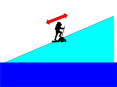
This game should be easy to solve. There exists a threshold above which the agent should always choose to go left and below which it should always go right. And yet a DQN agent will periodically die. Initially, the DQN quickly learns a good policy and avoids the catastrophe, but over the course of continued training, the agent, owing to the shape of the reward function, collapses to a policy which always moves right, regardless of the state. We might critically ask in what real-world scenario, we could depend upon a system that cannot solve Adventure Seeker.

Cart-Pole

In this classic RL environment, an agent balances a pole atop a cart (Figure 1(b)). Qualitatively, the game exhibits four distinct catastrophe modes. The pole could fall down to the right or fall down to the left. Additionally, the cart could run off the right boundary of the screen or run off the left. Formally, at each time, the agent observes a four-dimensional state vector $(x,v,\theta,\omega)$ consisting respectively of the cart position, cart velocity, pole angle, and the pole’s angular velocity. At each time step, the agent chooses an action, applying a force of either $-1$ or $+1$. For every time step that the pole remains upright and the cart remains on the screen, the agent receives a reward of $1$. If the pole falls, the episode terminates, giving a return of $0$ from the penultimate state. In experiments, we use the implementation CartPole-v0 contained in the openAI gym [6]. Like Adventure Seeker, this problem admits an analytic solution. A perfect policy should never drop the pole. But, as with Adventure Seeker, a DQN converges to a constant rate of catastrophes per turn.

Atari games

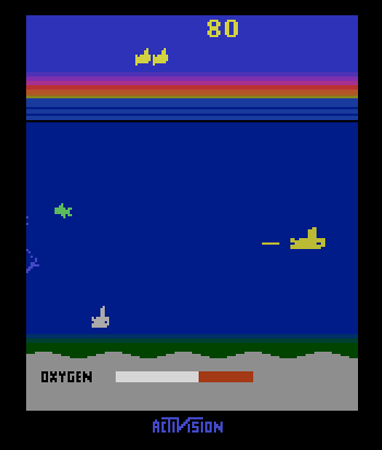
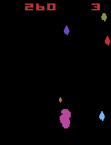
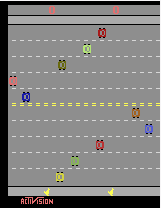
In addition to these pathological cases, we address Freeway, Asteroids, and Seaquest, games from the Atari Learning Environment. In Freeway, the agent controls a chicken with a goal of crossing the road while dodging traffic. The chicken loses a life and starts from the original location if hit by a car. Points are only rewarded for successfully crossing the road. In Asteroids, the agent pilots a ship and gains points from shooting the asteroids. She must avoid colliding with asteroids which cost it lives. In Seaquest, a player swims under water. Periodically, as the oxygen gets low, she must rise to the surface for oxygen. Additionally, fishes swim across the screen. The player gains points each time she shoots a fish. Colliding with a fish or running out of oxygen result in death. In all three games, the agent has 3 lives, and the final death is a terminal state. We label each loss of a life as a catastrophe state.

5 Experiments

First, on the toy examples, We evaluate standard DQNs and intrinsic fear DQNs using multilayer perceptrons (MLPs) with a single hidden layer and $128$ hidden nodes. We train all MLPs by stochastic gradient descent using the Adam optimizer [16].

In Adventure Seeker, an agent can escape from danger with only a few time steps of notice, so we set the fear radius $k_{r}$ to $5$. We phase in the fear factor quickly, reaching full strength in just $1000$ steps. On this problem we set the fear factor $\lambda$ to $40$. For Cart-Pole, we set a wider fear radius of $k_{r}=20$. We initially tried training this model with a short fear radius but made the following observation: One some runs, IF-DQN would surviving for millions of experiences, while on other runs, it might experience many catastrophes. Manually examining fear model output on successful vs unsuccessful runs, we noticed that on the bad runs, the fear model outputs non-zero probability of danger for precisely the $5$ moves before a catastrophe. In Cart-Pole, by that time, it is too to correct course. On the more successful runs, the fear model often outputs predictions in the range $.1-.5$. We suspect that the gradation between mildly dangerous states and those with certain danger provides a richer reward signal to the DQN.

On both the Adventure Seeker and Cart-Pole environments, DQNs augmented by intrinsic fear far outperform their otherwise identical counterparts. We also compared IF to some traditional approaches for mitigating catastrophic forgetting. For example, we tried a memory-based method in which we preferentially sample the catastrophic states for updating the model, but they did not improve over the DQN. It seems that the notion of a danger zone is necessary here.

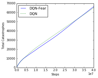
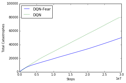
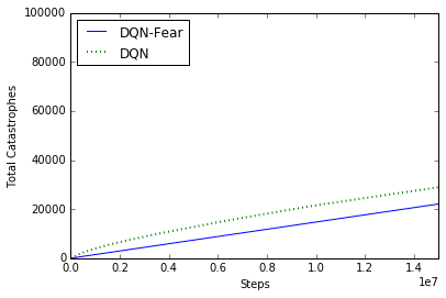
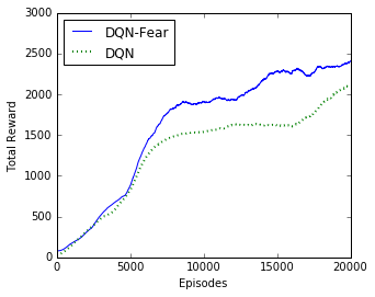
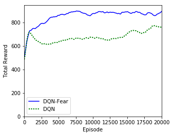
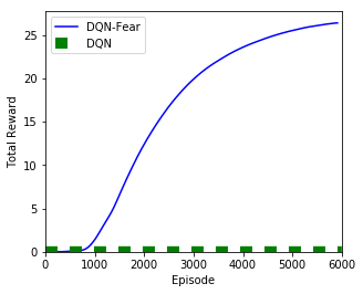
For Seaquest, Asteroids, and Freeway, we use a fear radius of $5$ and a fear factor of $.5$. For all Atari games, the IF models outperform their DQN counterparts. Interestingly while for all games, the IF models achieve higher reward, on Seaquest, IF-DQNs have similar catastrophe rates (Figure 2). Perhaps the IF-DQN enters a region of policy space with a strong incentives to exchange catastrophes for higher reward. This result suggests an interplay between the various reward signals that warrants further exploration. For Asteroids and Freeway, the improvements are more dramatic. Over just a few thousand episodes of Freeway, a randomly exploring DQN achieves zero reward. However, the reward shaping of intrinsic fear leads to rapid improvement.

(a) Seaquest

(b) Asteroids

(c) Freeway

(d) Seaquest

(e) Asteroids

(f) Freeway

Figure 2: Catastrophes (first row) and reward/episode (second row) for DQNs and Intrinsic Fear. On Adventure Seeker, all Intrinsic Fear models cease to “die” within $14$ runs, giving unbounded (unplottable) reward thereafter. On Seaquest, the IF model achieves a similar catastrophe rate but significantly higher total reward. On Asteroids, the IF model outperforms DQN. For Freeway, a randomly exploring DQN (under our time limit) never gets reward but IF model learns successfully.

6 Related work

The paper studies safety in RL, intrinsically motivated RL, and the stability of Q-learning with function approximation under distributional shift. Our work also has some connection to reward shaping. We attempt to highlight the most relevant papers here. Several papers address safety in RL. Garcıa and Fernández [2015] provide a thorough review on the topic, identifying two main classes of methods: those that perturb the objective function and those that use external knowledge to improve the safety of exploration.

While a typical reinforcement learner optimizes expected return, some papers suggest that a safely acting agent should also minimize risk. Hans et al. [2008] defines a fatality as any return below some threshold $\tau$. They propose a solution comprised of a safety function, which identifies unsafe states, and a backup model, which navigates away from those states. Their work, which only addresses the tabular setting, suggests that an agent should minimize the probability of fatality instead of maximizing the expected return. Heger [1994] suggests an alternative Q-learning objective concerned with the minimum (vs. expected) return. Other papers suggest modifying the objective to penalize policies with high-variance returns [10, 8]. Maximizing expected returns while minimizing their variance is a classic problem in finance, where a common objective is the ratio of expected return to its standard deviation [28]. Moreover, Azizzadenesheli et al. [2018] suggests to learn the variance over the returns in order to make safe decisions at each decision step. Moldovan and Abbeel [2012] give a definition of safety based on ergodicity. They consider a fatality to be a state from which one cannot return to the start state. Shalev-Shwartz et al. [2016] theoretically analyzes how strong a penalty should be to discourage accidents. They also consider hard constraints to ensure safety. None of the above works address the case where distributional shift dooms an agent to perpetually revisit known catastrophic failure modes. Other papers incorporate external knowledge into the exploration process. Typically, this requires access to an oracle or extensive prior knowledge of the environment. In the extreme case, some papers suggest confining the policy search to a known subset of safe policies. For reasonably complex environments or classes of policies, this seems infeasible.

The potential oscillatory or divergent behavior of Q-learners with function approximation has been previously identified [5, 2, 11]. Outside of RL, the problem of covariate shift has been extensively studied [30]. Murata and Ozawa [2005] addresses the problem of catastrophic forgetting owing to distributional shift in RL with function approximation, proposing a memory-based solution. Many papers address intrinsic rewards, which are internally assigned, vs the standard (extrinsic) reward. Typically, intrinsic rewards are used to encourage exploration [26, 4] and to acquire a modular set of skills [7]. Some papers refer to the intrinsic reward for discovery as curiosity. Like classic work on intrinsic motivation, our methods perturb the reward function. But instead of assigning bonuses to encourage discovery of novel transitions, we assign penalties to discourage catastrophic transitions.

Key differences

In this paper, we undertake a novel treatment of safe reinforcement learning, While the literature offers several notions of safety in reinforcement learning, we see the following problem: Existing safety research that perturbs the reward function requires little foreknowledge, but fundamentally changes the objective globally. On the other hand, processes relying on expert knowledge may presume an unreasonable level of foreknowledge. Moreover, little of the prior work on safe reinforcement learning, to the best of our knowledge, specifically addresses the problem of catastrophic forgetting. This paper proposes a new class of algorithms for avoiding catastrophic states and a theoretical analysis supporting its robustness.

7 Conclusions

Our experiments demonstrate that DQNs are susceptible to periodically repeating mistakes, however bad, raising questions about their real-world utility when harm can come of actions. While it is easy to visualize these problems on toy examples, similar dynamics are embedded in more complex domains. Consider a domestic robot acting as a barber. The robot might receive positive feedback for giving a closer shave. This reward encourages closer contact at a steeper angle. Of course, the shape of this reward function belies the catastrophe lurking just past the optimal shave. Similar dynamics might be imagines in a vehicle that is rewarded for traveling faster but could risk an accident with excessive speed. Our results with the intrinsic fear model suggest that with only a small amount of prior knowledge (the ability to recognize catastrophe states after the fact), we can simultaneously accelerate learning and avoid catastrophic states. This work is a step towards combating DRL’s tendency to revisit catastrophic states due to catastrophic forgetting.

An extension to the Theorem 2

In practice, we gradually learn and improve $\widehat{F}$ where the difference between learned $\widehat{F}$ after two consecrative updates, $\widehat{F}_{t}$ and $\widehat{F}_{t+1}$, consequently, $\omega^{\pi^{*}_{\widehat{F}_{t},\gamma_{plan}}}$ and $\omega^{\pi^{*}_{\widehat{F}_{t+1},\gamma_{plan}}}$ decrease. While $\widehat{F}_{t+1}$ is learned through using the samples drawn from $\omega^{\pi^{*}_{\widehat{F}_{t},\gamma_{plan}}}$, with high probability

$$\int_{s\in\mathcal{S}}\omega^{\pi^{*}_{\widehat{F}_{t},\gamma_{plan}}}(s)\left|{F}(s)-\widehat{F}_{t+1}(s)\right|ds\leq 3200\frac{\mathcal{VC}(\mathcal{F})+\log{\frac{1}{\delta}}}{N}$$

But in the final bound in Theorem 2, we interested in $\int_{s\in\mathcal{S}}\omega^{\pi^{*}_{\widehat{F}_{t+1},\gamma_{plan}}}(s)\left|{F}(s)-\widehat{F}_{t+1}(s)\right|ds$. Via decomposing in into two terms

$$\int_{s\in\mathcal{S}}\omega^{\pi^{*}_{\widehat{F}_{t},\gamma_{plan}}}(s)\left|{F}(s)-\widehat{F}_{t+1}(s)\right|ds+\int_{s\in\mathcal{S}}|\omega^{\pi^{*}_{\widehat{F}_{t+1},\gamma_{plan}}}(s)-\omega^{\pi^{*}_{\widehat{F}_{t},\gamma_{plan}}}(s)|ds$$

Therefore, an extra term of $\lambda\frac{1}{1-\gamma_{plan}}\int_{s\in\mathcal{S}}|\omega^{\pi^{*}_{\widehat{F}_{t+1},\gamma_{plan}}}(s)-\omega^{\pi^{*}_{\widehat{F}_{t},\gamma_{plan}}}(s)|ds$ appears in the final bound of Theorem 2.

Regarding the choice of $\gamma_{plan}$, if $\lambda\frac{\mathcal{VC}(\mathcal{F})+\log{\frac{1}{\delta}}}{N}$ is less than one, then the best choice of $\gamma_{plan}$ is $\gamma$. Other wise, if $\frac{\mathcal{VC}(\mathcal{F})+\log{\frac{1}{\delta}}}{N}$ is equal to exact error in the model estimation, and is greater than $1$, then the best $\gamma_{plan}$ is 0. Since, $\frac{\mathcal{VC}(\mathcal{F})+\log{\frac{1}{\delta}}}{N}$ is an upper bound, not an exact error, on the model estimation, the choice of zero for $\gamma_{plan}$ is not recommended, and a choice of $\gamma_{plan}\leq\gamma$ is preferred.

References

- Azizzadenesheli et al. [2018] Kamyar Azizzadenesheli, Emma Brunskill, and Animashree Anandkumar. Efficient exploration through bayesian deep q-networks. arXiv preprint arXiv:1802.04412, 2018.
- Baird [1995] Leemon Baird. Residual algorithms: Reinforcement learning with function approximation. 1995.
- Bellemare et al. [2013] Marc G Bellemare, Yavar Naddaf, Joel Veness, and Michael Bowling. The arcade learning environment: An evaluation platform for general agents. J. Artif. Intell. Res.(JAIR), 2013.
- Bellemare et al. [2016] Marc G Bellemare, Sriram Srinivasan, Georg Ostrovski, Tom Schaul, David Saxton, and Remi Munos. Unifying count-based exploration and intrinsic motivation. In NIPS, 2016.
- Boyan and Moore [1995] Justin Boyan and Andrew W Moore. Generalization in reinforcement learning: Safely approximating the value function. In NIPS, 1995.
- Brockman et al. [2016] Greg Brockman, Vicki Cheung, Ludwig Pettersson, Jonas Schneider, John Schulman, Jie Tang, and Wojciech Zaremba. OpenAI gym, 2016. arxiv.org/abs/1606.01540.
- Chentanez et al. [2004] Nuttapong Chentanez, Andrew G Barto, and Satinder P Singh. Intrinsically motivated reinforcement learning. In NIPS, 2004.
- Chow et al. [2015] Yinlam Chow, Aviv Tamar, Shie Mannor, and Marco Pavone. Risk-sensitive and robust decision-making: A CVaR optimization approach. In NIPS, 2015.
- Fatemi et al. [2016] Mehdi Fatemi, Layla El Asri, Hannes Schulz, Jing He, and Kaheer Suleman. Policy networks with two-stage training for dialogue systems. In SIGDIAL, 2016.
- Garcıa and Fernández [2015] Javier Garcıa and Fernando Fernández. A comprehensive survey on safe reinforcement learning. JMLR, 2015.
- Gordon [1996] Geoffrey J Gordon. Chattering in SARSA(). Technical report, CMU, 1996.
- Hanneke [2016] Steve Hanneke. The optimal sample complexity of PAC learning. JMLR, 2016.
- Hans et al. [2008] Alexander Hans, Daniel Schneegaß, Anton Maximilian Schäfer, and Steffen Udluft. Safe exploration for reinforcement learning. In ESANN, 2008.
- Heger [1994] Matthias Heger. Consideration of risk in reinforcement learning. In Machine Learning, 1994.
- Jiang et al. [2015] Nan Jiang, Alex Kulesza, Satinder Singh, and Richard Lewis. The dependence of effective planning horizon on model accuracy. In International Conference on Autonomous Agents and Multiagent Systems, 2015.
- Kingma and Ba [2015] Diederik Kingma and Jimmy Ba. Adam: A method for stochastic optimization. In ICLR, 2015.
- Levine et al. [2016] Sergey Levine, Chelsea Finn, Trevor Darrell, and Pieter Abbeel. End-to-end training of deep visuomotor policies. JMLR, 2016.
- Lin [1992] Long-Ji Lin. Self-improving reactive agents based on reinforcement learning, planning and teaching. Machine learning, 1992.
- Lipton et al. [2018] Zachary C Lipton, Jianfeng Gao, Lihong Li, Xiujun Li, Faisal Ahmed, and Li Deng. Efficient exploration for dialogue policy learning with bbq networks & replay buffer spiking. In AAAI, 2018.
- McClelland et al. [1995] James L McClelland, Bruce L McNaughton, and Randall C O’Reilly. Why there are complementary learning systems in the hippocampus and neocortex: Insights from the successes and failures of connectionist models of learning and memory. Psychological Review, 1995.
- McCloskey and Cohen [1989] Michael McCloskey and Neal J Cohen. Catastrophic interference in connectionist networks: The sequential learning problem. Psychology of learning and motivation, 1989.
- Mnih et al. [2015] Volodymyr Mnih et al. Human-level control through deep reinforcement learning. Nature, 2015.
- Moldovan and Abbeel [2012] Teodor Mihai Moldovan and Pieter Abbeel. Safe exploration in Markov decision processes. In ICML, 2012.
- Murata and Ozawa [2005] Makoto Murata and Seiichi Ozawa. A memory-based reinforcement learning model utilizing macro-actions. In Adaptive and Natural Computing Algorithms. 2005.
- Night [2016] Will Night. The AI that cut google’s energy bill could soon help you. MIT Tech Review, 2016.
- Schmidhuber [1991] Jurgen Schmidhuber. A possibility for implementing curiosity and boredom in model-building neural controllers. In From animals to animats: SAB90, 1991.
- Shalev-Shwartz et al. [2016] Shai Shalev-Shwartz, Shaked Shammah, and Amnon Shashua. Safe, multi-agent, reinforcement learning for autonomous driving. 2016.
- Sharpe [1966] William F Sharpe. Mutual fund performance. The Journal of Business, 1966.
- Silver et al. [2016] David Silver et al. Mastering the game of go with deep neural networks and tree search. Nature, 2016.
- Sugiyama and Kawanabe [2012] Masashi Sugiyama and Motoaki Kawanabe. Machine learning in non-stationary environments: Introduction to covariate shift adaptation. MIT Press, 2012.
- Sutton [1988] Richard S. Sutton. Learning to predict by the methods of temporal differences. Machine Learning, 1988.
- Vapnik [2013] Vladimir Vapnik. The nature of statistical learning theory. Springer science & business media, 2013.
- Watkins and Dayan [1992] Christopher J.C.H. Watkins and Peter Dayan. -learning. Machine Learning, 1992.