Demystifying ResNet
Abstract
The Residual Network (ResNet), proposed in He et al. (2015a), utilized shortcut connections to significantly reduce the difficulty of training, which resulted in great performance boosts in terms of both training and generalization error.
It was empirically observed in He et al. (2015a) that stacking more layers of residual blocks with shortcut results in smaller training error, while it is not true for shortcut of length or . We provide a theoretical explanation for the uniqueness of shortcut .
We show that with or without nonlinearities, by adding shortcuts that have depth two, the condition number of the Hessian of the loss function at the zero initial point is depth-invariant, which makes training very deep models no more difficult than shallow ones. Shortcuts of higher depth result in an extremely flat (high-order) stationary point initially, from which the optimization algorithm is hard to escape. The shortcut , however, is essentially equivalent to no shortcuts, which has a condition number exploding to infinity as the number of layers grows. We further argue that as the number of layers tends to infinity, it suffices to only look at the loss function at the zero initial point.
Extensive experiments are provided accompanying our theoretical results. We show that initializing the network to small weights with shortcut achieves significantly better results than random Gaussian (Xavier) initialization, orthogonal initialization, and shortcuts of deeper depth, from various perspectives ranging from final loss, learning dynamics and stability, to the behavior of the Hessian along the learning process.
1 Introduction
Residual network (ResNet) was first proposed in He et al. (2015a) and extended in He et al. (2016). It followed a principled approach to add shortcut connections every two layers to a VGG-style network (Simonyan and Zisserman, 2014). The new network becomes easier to train, and achieves both lower training and test errors. Using the new structure, He et al. (2015a) managed to train a network with 1001 layers, which was virtually impossible before. Unlike Highway Network (Srivastava et al., 2015a, b) which not only has shortcut paths but also borrows the idea of gates from LSTM (Sainath et al., 2015), ResNet does not have gates. Later He et al. (2016) found that by keeping a clean shortcut path, residual networks will perform even better.
Many attempts have been made to improve ResNet to a further extent. “ResNet in ResNet” (Targ et al., 2016) adds more convolution layers and data paths to each layer, making it capable of representing several types of residual units. “ResNets of ResNets” (Zhang et al., 2016) construct multi-level shortcut connections, which means there exist shortcuts that skip multiple residual units. Wide Residual Networks (Zagoruyko and Komodakis, 2016) makes the residual network shorter but wider, and achieves state of the art results on several datasets while using a shallower network. Moreover, some existing models are also reported to be improved by shortcut connections, including Inception-v4 (Szegedy et al., 2016), in which shortcut connections make the deep network easier to train.
Understanding why the shortcut connections in ResNet could help reduce the training difficulty is an important question. Indeed, He et al. (2015a) suggests that layers in residual networks are learning residual mappings, making them easier to represent identity mappings, which prevents the networks from degradation when the depths of the networks increase. However, Veit et al. (2016) claims that ResNets are actually ensembles of shallow networks, which means they do not solve the problem of training deep networks completely. In Hardt and Ma (2016), they showed that for deep linear residual networks with shortcut does not have spurious local minimum, and analyzed and experimented with a new ResNet architecture with shortcut .
We would like to emphasize that it is not true that every type of identity mapping and shortcut works. Quoting He et al. (2015a):
“But if has only a single layer, Eqn.(1) is similar to a linear layer: , for which we have not observed advantages.”
“Deeper non-bottleneck ResNets (e.g., Fig. 5 left) also gain accuracy from increased depth (as shown on CIFAR-10), but are not as economical as the bottleneck ResNets. So the usage of bottleneck designs is mainly due to practical considerations. We further note that the degradation problem of plain nets is also witnessed for the bottleneck designs. ”
Their empirical observations are inspiring. First, the shortcut mentioned in the first paragraph do not work. It clearly contradicts the theory in Hardt and Ma (2016), which forces us to conclude that the nonlinear network behaves essentially in a different manner from the linear network. Second, noting that the non-bottleneck ResNets have shortcut , but the bottleneck ResNets use shortcut , one sees that shortcuts with depth three also do not ease the optimization difficulties.
In light of these empirical observations, it is sensible to say that a reasonable theoretical explanation must be able to distinguish shortcut from shortcuts of other depths, and clearly demonstrate why shortcut is special and is able to ease the optimization process so significantly for deep models, while shortcuts of other depths may not do the job. Moreover, analyzing deep linear models may not be able to provide the right intuitions.
2 Main results
We provide a theoretical explanation for the unique role of shortcut of length . Our arguments can be decomposed into two parts.
-
1.
For very deep (general) ResNet, it suffices to initialize the weights at zero and search locally: in other words, there exist a global minimum whose weight functions for each layer have vanishing norm as the number of layers tends to infinity.
-
2.
For very deep (general) ResNet, the loss function at the zero initial point exhibits radically different behavior for shortcuts of different lengths. In particular, the Hessian at the zero initial point for the -shortcut network has condition number growing unboundedly when the number of layers grows, while the -shortcut network enjoys a depth-invariant condition number. ResNet with shortcut length larger than has the zero initial point as a high order saddle point (with Hessian a zero matrix), which may be difficult to escape from in general.
We provide extensive experiments validating our theoretical arguments. It is mathematically surprising to us that although the deep linear residual networks with shortcut has no spurious local minimum (Hardt and Ma, 2016), this result does not generalize to the nonlinear case and the training difficulty is not reduced. Deep residual network of shortcut length admits spurious local minimum in general (such as the zero initial point), but proves to work in practice.
As a side product, our experiments reveal that orthogonal initialization (Saxe et al., 2013) is suboptimal. Although better than Xavier initialization (Glorot and Bengio, 2010), the initial condition numbers of the networks still explode as the networks become deeper, which means the networks are still initialized on “bad” submanifolds that are hard to optimize using gradient descent.
3 Model
We first generalize a linear network by adding shortcuts to it to make it a linear residual network. We organize the network into residual units. The -th residual unit consists of layers whose weights are , denoted as the transformation path, as well as a shortcut connecting from the first layer to the last one, denoted as the shortcut path. The input-output mapping can be written as
| (1) |
where . Here if , denotes , otherwise it denotes an identity mapping. The matrix represents the combination of all the linear transformations in the network. Note that by setting all the shortcuts to zeros, the network will go back to a -layer plain linear network.
Instead of analyzing the general form, we concentrate on a special kind of linear residual networks, where all the residual units are the same.
Definition 1.
A linear residual network is called an -shortcut linear network if
-
1.
its layers have the same dimension (so that );
-
2.
its shortcuts are identity matrices;
-
3.
its shortcuts have the same depth .
The input-output mapping for such a network becomes
| (2) |
where .
Then we add some activation functions to the networks. We concentrate on the case where activation functions are on the transformation paths, which is also the case in the latest ResNet (He et al., 2016).
Definition 2.
An -shortcut linear network becomes an -shortcut network if element-wise activation functions are added at the transformation paths, where on a transformation path, is added before the first weight matrix, is added between two weight matrices and is added after the last weight matrix.

Note that -shortcut linear networks are special cases of -shortcut networks, where all the activation functions are identity mappings.
4 Theoretical study
4.1 Small weights property of (near) global minimum
ResNet uses MSRA initialization (He et al., 2015b). It is a kind of scaled Gaussian initialization that tries to keep the variances of signals along a transformation path, which is also the idea behind Xavier initialization (Glorot and Bengio, 2010). However, because of the shortcut paths, the output variance of the entire network will actually explode as the network becomes deeper. Batch normalization units partly solved this problem in ResNet, but still they cannot prevent the large output variance in a deep network.
A simple idea is to zero initialize all the weights, so that the output variances of residual units stay the same along the network. It is worth noting that as found in He et al. (2015a), the deeper ResNet has smaller magnitudes of layer responses. This phenomenon has been confirmed in our experiments. As illustrated in Figure 2 and Figure 3, the deeper a residual network is, the small its average Frobenius norm of weight matrices is, both during the training process and when the training ends. Also, Hardt and Ma (2016) proves that if all the weight matrices have small norms, a linear residual network with shortcut of length will have no critical points other than the global optimum.
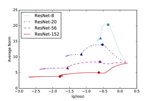
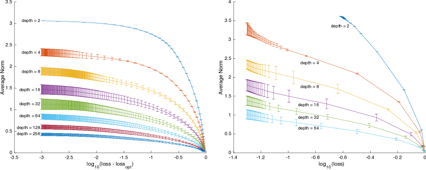
All these evidences indicate that zero is special in a residual network: as the network becomes deeper, the training tends to end up around it. Thus, we are looking into the Hessian at zero. As the zero is a saddle point, in our experiments we use zero initialization with small random perturbations to escape from it. We first Xavier initialize the weight matrices, and then multiply a small constant () to them.
Now we present a simplified ResNet structure with shortcut of length , and prove that as the residual network becomes deeper, there exists a solution whose weight functions have vanishing norm, which is observed in ResNet as we mentioned. This argument is motivated by Hardt and Ma (2016).
We concentrate on a special kind of network whose overall transformation can be written as
| (3) |
where is the bias term. It can seen as a simplified version of ResNet (He et al., 2016). Note that although this network is not a -shortcut network, its Hessian still follow the form of Theorem 2, thus its condition number is still depth-invariant.
We will also make some assumptions on the training samples.
Assumption 1.
Assume , for every , where are standard basis vectors in .
The formats of training samples describe above are common in practice, where the input data are whitened and the labels are one-hot encoded. Furthermore, we borrow an mild assumption from Hardt and Ma (2016) that there exists a minimum distance between every two data points.
Definition 3.
The minimum distance of a group of vectors is defined as
| (4) |
where .
Assumption 2.
There exists a minimum distance between all the sample points and all the labels, i.e.
| (5) |
As pointed out in Hardt and Ma (2016), this assumption can be satisfied by adding a small noise to the dataset. Given the model and the assumptions, we are ready to present our theorem whose proof can be found in Appendix A.1.
Theorem 1.
For a specific dataset, are fixed, so the above equation can be simplified to
| (7) |
This indicates that as the network become deeper, there exists a solution that is closer to the zero. As a result, it is possible that in a zero initialized deep residual network, the weights are not far from the initial point throughout the training process, where the condition number is small, making it easy for gradient decent to optimize the network.
4.2 Special properties of shortcut at zero initial point
We begin with the definition of -th order stationary point.
Definition 4.
Suppose function admits -th order Taylor expansion at point . We say that the point is a -th order stationary point of if the corresponding -th order Taylor expansion of at is a constant: .
Then we make some assumptions on the activation functions.
Assumption 3.
and all of exist.
The assumptions hold for most activation functions including tanh, symmetric sigmoid and ReLU (Nair and Hinton, 2010). Note that although ReLU does not have derivatives at zero, one may do a local polynomial approximation to yield .
Now we state our main theorem, whose proof can be found in Appendix A.2.
Theorem 2.
Suppose all the activation functions satisfy Assumption 3. For the loss function of an -shortcut network, at point zero,
-
1.
if , it is an th-order stationary point. In particular, if , the Hessian is a zero matrix;
-
2.
if , the Hessian can be written as
(8) whose condition number is
(9) where only depends on the training set and the activation functions. Except for degenerate cases, it is a strict saddle point (Ge et al., 2015).
-
3.
if , the Hessian can be written as
(10) where only depend on the training set and the activation functions.
Theorem 2 shows that the condition numbers of -shortcut networks are depth-invariant with a nice structure of eigenvalues. Indeed, the eigenvalues of the Hessian at the zero initial point are multiple copies of , and the number of copies is equal to the number of shortcut connections.
The Hessian at zero initial point for the -shortcut network follows block Toeplitz structure, which has been well studied in the literature. In particular, its condition number tends to explode as the number of layers increase (Gray, 2006).
To get intuitive explanations of the theorem, imagine changing parameters in an -shortcut network. One has to change at least parameters to make any difference in the loss. So zero is an th-order stationary point. Notice that the higher the order of a stationary point, the more difficult for a first order method to escape from it.
On the other hand, if , one will have to change two parameters in the same residual unit but different weight matrices to affect the loss, leading to a clear block diagonal Hessian.
5 Experiments
We compare networks with Xavier initialization (Glorot and Bengio, 2010), networks with orthogonal initialization (Saxe et al., 2013) and -shortcut networks with zero initialization. The training dynamics of -shortcut networks are similar to that of linear networks with orthogonal initialization in our experiments. Setup details can be found in Appendix B.
5.1 Initial point
We first compute the initial condition numbers for different kinds of linear networks with different depths.
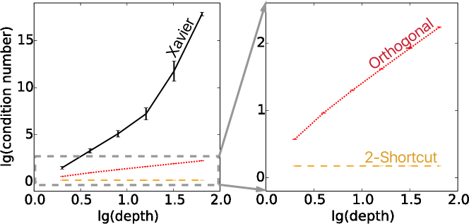
As can be seen in Figure 4, -shortcut linear networks have constant condition numbers as expected. On the other hand, when using Xavier or orthogonal initialization in linear networks, the initial condition numbers will go to infinity as the depths become infinity, making the networks hard to train. This also explains why orthogonal initialization is helpful for a linear network, as its initial condition number grows slower than the Xavier initialization.
5.2 Learning dynamics
Having a good beginning does not guarantee an easy trip on the loss surface. In order to depict the loss surfaces encountered from different initial points, we plot the maxima and 10th percentiles (instead of minima, as they are very unstable) of the absolute values of Hessian’s eigenvalues at different losses.
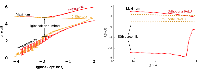
As shown in Figure 5, the condition numbers of -shortcut networks at different losses are always smaller, especially when the loss is large. Also, notice that the condition numbers roughly evolved to the same value for both orthogonal and -shortcut linear networks. This may be explained by the fact that the minimizers, as well as any point near them, have similar condition numbers.
Another observation is the changes of negative eigenvalues ratios. Index (ratio of negative eigenvalues) is an important characteristic of a critical point. Usually for the critical points of a neural network, the larger the loss the larger the index (Dauphin et al., 2014). In our experiments, the index of a -shortcut network is always smaller, and drops dramatically at the beginning, as shown in Figure 6, left. This might make the networks tend to stop at low critical points.
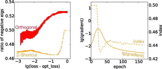
This is because the initial point is near a saddle point, thus it tends to go towards negative curvature directions, eliminating some negative eigenvalues at the beginning. This phenomenon matches the observation that the gradient reaches its maximum when the index drops dramatically, as shown in Figure 6, right.
5.3 Learning results
5.3.1 MNIST dataset
We run different networks for 1000 epochs using different learning rates at log scale, and compare the average final losses corresponding to the optimal learning rates.
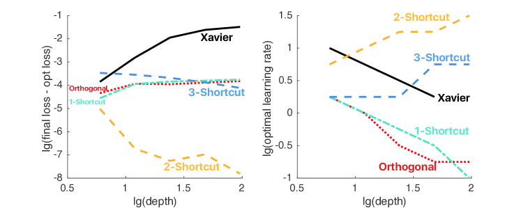
Figure 7 shows the results for linear networks. Just like their depth-invariant initial condition numbers, the final losses of -shortcut linear networks stay close to optimal as the networks become deeper. Higher learning rates can also be applied, resulting in fast learning in deep networks.
Then we add ReLUs to the mid positions of the networks. To make a fair comparison, the numbers of ReLU units in different networks are the same when the depths are the same, so -shortcut and -shortcut networks are omitted. The result is shown in Figure 8.
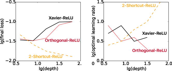
Note that because of the nonlinearities, the optimal losses vary for different networks with different depths. It is usually thought that deeper networks can represent more complex models, leading to smaller optimal losses. However, our experiments show that linear networks with Xavier or orthogonal initialization have difficulties finding these optimal points, while -shortcut networks find these optimal points easily as they did without nonlinear units.
5.3.2 CIFAR-10 dataset
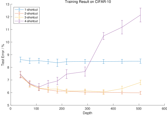
To show the effect of shortcut depth on a larger dataset, we modify the pre-ResNet implementation in https://github.com/facebook/fb.resnet.torch to make it possible to change shortcut depth while keeping the total number of parameters fixed. The default stopping criteria are used. The result is shown in Figure 9. As shown in the figure, when the network becomes extremely deep (), only ResNets with shortcut gain advantages from the growth of depth, where other networks suffer from degradation as the network becomes deeper.
References
- Bishop (1992) Chris Bishop. Exact calculation of the hessian matrix for the multilayer perceptron, 1992.
- Dauphin et al. (2014) Yann N Dauphin, Razvan Pascanu, Caglar Gulcehre, Kyunghyun Cho, Surya Ganguli, and Yoshua Bengio. Identifying and attacking the saddle point problem in high-dimensional non-convex optimization. In Advances in neural information processing systems, pages 2933–2941, 2014.
- Ge et al. (2015) Rong Ge, Furong Huang, Chi Jin, and Yang Yuan. Escaping from saddle points—online stochastic gradient for tensor decomposition. In Proceedings of The 28th Conference on Learning Theory, pages 797–842, 2015.
- Glorot and Bengio (2010) Xavier Glorot and Yoshua Bengio. Understanding the difficulty of training deep feedforward neural networks. In Aistats, volume 9, pages 249–256, 2010.
- Gray (2006) Robert M Gray. Toeplitz and circulant matrices: A review. now publishers inc, 2006.
- Hardt and Ma (2016) Moritz Hardt and Tengyu Ma. Identity matters in deep learning. arXiv preprint arXiv:1611.04231, 2016.
- He et al. (2015a) Kaiming He, Xiangyu Zhang, Shaoqing Ren, and Jian Sun. Deep residual learning for image recognition. arXiv preprint arXiv:1512.03385, 2015a.
- He et al. (2015b) Kaiming He, Xiangyu Zhang, Shaoqing Ren, and Jian Sun. Delving deep into rectifiers: Surpassing human-level performance on imagenet classification. In Proceedings of the IEEE International Conference on Computer Vision, pages 1026–1034, 2015b.
- He et al. (2016) Kaiming He, Xiangyu Zhang, Shaoqing Ren, and Jian Sun. Identity mappings in deep residual networks. arXiv preprint arXiv:1603.05027, 2016.
- Nair and Hinton (2010) Vinod Nair and Geoffrey E Hinton. Rectified linear units improve restricted boltzmann machines. In Proceedings of the 27th International Conference on Machine Learning (ICML-10), pages 807–814, 2010.
- Sainath et al. (2015) Tara N Sainath, Oriol Vinyals, Andrew Senior, and Haşim Sak. Convolutional, long short-term memory, fully connected deep neural networks. In Acoustics, Speech and Signal Processing (ICASSP), 2015 IEEE International Conference on, pages 4580–4584. IEEE, 2015.
- Saxe et al. (2013) Andrew M Saxe, James L McClelland, and Surya Ganguli. Exact solutions to the nonlinear dynamics of learning in deep linear neural networks. arXiv preprint arXiv:1312.6120, 2013.
- Simonyan and Zisserman (2014) Karen Simonyan and Andrew Zisserman. Very deep convolutional networks for large-scale image recognition. arXiv preprint arXiv:1409.1556, 2014.
- Srivastava et al. (2015a) Rupesh K Srivastava, Klaus Greff, and Jürgen Schmidhuber. Training very deep networks. In Advances in neural information processing systems, pages 2377–2385, 2015a.
- Srivastava et al. (2015b) Rupesh Kumar Srivastava, Klaus Greff, and Jürgen Schmidhuber. Highway networks. arXiv preprint arXiv:1505.00387, 2015b.
- Szegedy et al. (2016) Christian Szegedy, Sergey Ioffe, Vincent Vanhoucke, and Alex Alemi. Inception-v4, inception-resnet and the impact of residual connections on learning. arXiv preprint arXiv:1602.07261, 2016.
- Targ et al. (2016) Sasha Targ, Diogo Almeida, and Kevin Lyman. Resnet in resnet: Generalizing residual architectures. arXiv preprint arXiv:1603.08029, 2016.
- Veit et al. (2016) Andreas Veit, Michael Wilber, and Serge Belongie. Residual networks are exponential ensembles of relatively shallow networks. arXiv preprint arXiv:1605.06431, 2016.
- Zagoruyko and Komodakis (2016) Sergey Zagoruyko and Nikos Komodakis. Wide residual networks. arXiv preprint arXiv:1605.07146, 2016.
- Zhang et al. (2016) Ke Zhang, Miao Sun, Tony X Han, Xingfang Yuan, Liru Guo, and Tao Liu. Residual networks of residual networks: Multilevel residual networks. arXiv preprint arXiv:1608.02908, 2016.
Appendix A Proofs of theorems
A.1 Proof of Theorem 1
Lemma 1.
Given matrix such that
| (11) | ||||
| (12) |
where and are unit vectors in , , . There exists such that
| (13) |
| (14) |
Lemma 1 constructs a residual unit that change one column of its input by . Now we are going to proof that by repeating this step, the input matrix can be transfered into the output matrix .
Lemma 2.
Given that , there exists a sequence of matrix where
| (18) |
| (19) |
such that for every , and conform to Lemma 1 with a distance smaller than .
Proof.
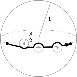
In order to complete the transformation, we can modify column by column. For each column vector, in order to move it while preserving a minimum distance, we can draw a minor arc on the unit sphere connecting the starting and the ending point, bypassing each obstacle by a minor arc with a radius of if needed, as shown in Figure 10. The length of the path is smaller than , thus steps are sufficient to keep each step shorter than . Repeating the process for times will give us a legal construction. ∎
Now we can prove Theorem 1 with the all these lemmas above.
A.2 Proof of Theorem 2
Definition 5.
The elements in Hessian of an -shortcut network is defined as
| (21) |
where is the loss function, and the indices is ordered lexicographically following the four indices of the weight variable . In other words, the priority decreases along the index of shortcuts, index of weight matrix inside shortcuts, index of column, and index of row.
Note that the collection of all the weight variables in the -shortcut network is denoted as . We study the behavior of the loss function in the vicinity of .
Lemma 3.
Assume that are parameters of an -shortcut network. If is nonzero, there exists and such that and for .
Proof.
Assume there does not exist such and , then for all the shortcut units , there exists a weight matrix such that none of is in , so all the transformation paths are zero, which means . Then , leading to a contradiction. ∎
Lemma 4.
Assume that . Let denotes the loss function with all the parameters except and set to 0, . Then .
Proof.
As all the residual units expect unit and are identity transformations, reordering residual units while preserving the order of units and will not affect the overall transformation, i.e. . So . ∎
Proof of Theorem 2.
Now we can prove Theorem 2 with the help of the previously established lemmas.
-
1.
Using Lemma 3, for an -shortcut network, at zero, all the -th order partial derivatives of the loss function are zero, where ranges from to . Hence, the initial point zero is a th-order stationary point of the loss function.
-
2.
Consider the Hessian in case. Using Lemma 3 and Lemma 4, the form of Hessian can be directly written as Equation (8), as illustrated in Figure 11.
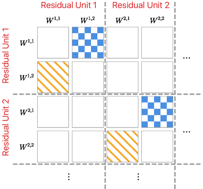
Figure 11: The Hessian in case. It follows from Lemma 3 that only off-diagonal subblocks in each diagonal block, i.e., the blocks marked in orange (slash) and blue (chessboard), are non-zero. From Lemma 4, we conclude the translation invariance and that all blocks marked in orange (slash) (resp. blue (chessboard)) are the same. Given that the Hessian is symmetric, the blocks marked in blue and orange are transposes of each other, and thus it can be directly written as Equation (8). So we have
(22) Thus , which is depth-invariant. Note that the dimension of is .
To get the expression of , consider two parameters that are in the same residual unit but different weight matrices, i.e. .
If , we have
(23) Else, we have .
Noting that in fact only depends on the two indices (with a small difference depending on whether ), we make a matrix with rows indexed by and columns indexed by , and the entry at equal to . Apparently, this matrix is equal to when , and equal to the zero matrix when .
To simplify the expression of , we rearrange the columns of by a permutation matrix, i.e.
(24) where if and only if . Basically it permutes the -th column of to the -th column.
Then we have
(25) So the eigenvalues of becomes
(26) which leads to Equation (9).
-
3.
Now consider the Hessian in the case. Using Lemma 4, the form of Hessian can be directly written as Equation (10).
To get the expressions of and in case, consider two parameters that are in the same residual units, i.e. .
We have
(27) (28) Rearrange the order of variables using , we have
(29) Then consider two parameters that are in different residual units, i.e. .
We have
(30) (31) In the same way, we can rewrite as
(32)
∎
Appendix B Experiment setup on MNIST
We took the experiments on whitened versions of MNIST. Ten greatest principal components are kept for the dataset inputs. The dataset outputs are represented using one-hot encoding. The network was trained using gradient descent. For every epoch, the Hessians of the networks were calculated using the method proposed in Bishop (1992). As the of Hessian is usually very unstable, we calculated to represent condition number instead, where is the 10th percentile of the absolute values of eigenvalues.
As pre, mid or post positions are not defined in linear networks without shortcuts, when comparing Xavier or orthogonal initialized linear networks to -shortcut networks, we added ReLUs at the same positions in linear networks as in -shortcuts networks.