Variational Inference via
$\chi$ Upper Bound Minimization

Abstract

Variational inference (vi) is widely used as an efficient alternative to Markov chain Monte Carlo. It posits a family of approximating distributions $q$ and finds the closest member to the exact posterior $p$. Closeness is usually measured via a divergence $D(q||p)$ from $q$ to $p$. While successful, this approach also has problems. Notably, it typically leads to underestimation of the posterior variance. In this paper we propose chivi, a black-box variational inference algorithm that minimizes $D_{\chi}(p||q)$, the $\chi$-divergence from $p$ to $q$. chivi minimizes an upper bound of the model evidence, which we term the $\chi$ upper bound (cubo). Minimizing the cubo leads to improved posterior uncertainty, and it can also be used with the classical vi lower bound (elbo) to provide a sandwich estimate of the model evidence. We study chivi on three models: probit regression, Gaussian process classification, and a Cox process model of basketball plays. When compared to expectation propagation and classical vi, chivi produces better error rates and more accurate estimates of posterior variance.

1 Introduction

Bayesian analysis provides a foundation for reasoning with probabilistic models. We first set a joint distribution $p(\boldsymbol{\mathbf{x}},\boldsymbol{\mathbf{z}})$ of latent variables $\boldsymbol{\mathbf{z}}$ and observed variables $\boldsymbol{\mathbf{x}}$. We then analyze data through the posterior, $p(\boldsymbol{\mathbf{z}}\,|\,\boldsymbol{\mathbf{x}})$. In most applications, the posterior is difficult to compute because the marginal likelihood $p(\boldsymbol{\mathbf{x}})$ is intractable. We must use approximate posterior inference methods such as Monte Carlo [1] and variational inference [2]. This paper focuses on variational inference.

Variational inference approximates the posterior using optimization. The idea is to posit a family of approximating distributions and then to find the member of the family that is closest to the posterior. Typically, closeness is defined by the Kullback-Leibler (kl) divergence $\operatorname{KL}(q\,\|\,p)$, where $q(\boldsymbol{\mathbf{z}};\boldsymbol{\mathbf{\lambda}})$ is a variational family indexed by parameters $\boldsymbol{\mathbf{\lambda}}$. This approach, which we call klvi, also provides the evidence lower bound (elbo), a convenient lower bound of the model evidence $\log p(\boldsymbol{\mathbf{x}})$.

klvi scales well and is suited to applications that use complex models to analyze large data sets [3]. But it has drawbacks. For one, it tends to favor underdispersed approximations relative to the exact posterior [4, 5]. This produces difficulties with light-tailed posteriors when the variational distribution has heavier tails. For example, klvi for Gaussian process classification typically uses a Gaussian approximation; this leads to unstable optimization and a poor approximation [6].

One alternative to klvi is expectation propagation (ep), which enjoys good empirical performance on models with light-tailed posteriors [7, 8]. Procedurally, ep reverses the arguments in the kl divergence and performs local minimizations of $\operatorname{KL}(p\,\|\,q)$; this corresponds to iterative moment matching on partitions of the data. Relative to klvi, ep produces overdispersed approximations. But ep also has drawbacks. It is not guaranteed to converge [7, Figure $3.6$]; it does not provide an easy estimate of the marginal likelihood; and it does not optimize a well-defined global objective [9].

In this paper we develop a new algorithm for approximate posterior inference, chivi. chivi minimizes the $\chi$-divergence from the posterior to the variational family,

$$\vspace{-0.25ex}D_{\chi^{2}}(p\,\|\,q)=\mathbb{E}_{q(\boldsymbol{\mathbf{z}};\boldsymbol{\mathbf{\lambda}})}\Big{[}\Big{(}\frac{p(\boldsymbol{\mathbf{z}}\,|\,\boldsymbol{\mathbf{x}})}{q(\boldsymbol{\mathbf{z}};\boldsymbol{\mathbf{\lambda}})}\Big{)}^{2}-1\Big{]}.\vspace{0.75ex}$$ (1)

chivi enjoys advantages of both ep and klvi. Like ep, it produces overdispersed approximations; like klvi, it optimizes a well-defined objective and estimates the model evidence.

As we mentioned, klvi optimizes a lower bound on the model evidence. The idea behind chivi is to optimize an upper bound, which we call the cubo. Minimizing the cubo is equivalent to minimizing the $\chi$-divergence. In providing an upper bound, chivi can be used (in concert with klvi) to sandwich estimate the model evidence. Sandwich estimates are useful for tasks like model selection [10]. Existing work on sandwich estimation relies on MCMC and only evaluates simulated data [11]. We derive a sandwich theorem (Section 2) that relates cubo and elbo. Section 3 demonstrates sandwich estimation on real data.

Aside from providing an upper bound, there are two additional benefits to chivi. First, it is a black-box inference algorithm [12] in that it does not need model-specific derivations and it is easy to apply to a wide class of models. It minimizes an upper bound in a principled way using unbiased reparameterization gradients [13, 14] of the exponentiated cubo.

Second, it is a viable alternative to ep. The $\chi$-divergence enjoys the same “zero-avoiding” behavior of ep, which seeks to place positive mass everywhere, and so chivi is useful when the kl divergence is not a good objective (such as for light-tailed posteriors). Unlike ep, chivi is guaranteed to converge; provides an easy estimate of the marginal likelihood; and optimizes a well-defined global objective. Section 3 shows that chivi outperforms klvi and ep for Gaussian process classification.

The rest of this paper is organized as follows. Section 2 derives the cubo, develops chivi, and expands on its zero-avoiding property that finds overdispersed posterior approximations. Section 3 applies chivi to Bayesian probit regression, Gaussian process classification, and a Cox process model of basketball plays. On Bayesian probit regression and Gaussian process classification, it yielded lower classification error than klvi and ep. When modeling basketball data with a Cox process, it gave more accurate estimates of posterior variance than klvi.

Related work.  The most widely studied variational objective is $\operatorname{KL}(q\,\|\,p)$. The main alternative is ep [15, 7], which locally minimizes $\operatorname{KL}(p\,\|\,q)$. Recent work revisits ep from the perspective of distributed computing [16, 17, 18] and also revisits [19], which studies local minimizations with the general family of $\alpha$-divergences [20, 21]. chivi relates to ep and its extensions in that it leads to overdispersed approximations relative to klvi. However, unlike [19, 20], chivi does not rely on tying local factors; it optimizes a well-defined global objective. In this sense, chivi relates to the recent work on alternative divergence measures for variational inference [21, 22].

A closely related work is [21]. They perform black-box variational inference using the reverse $\alpha$-divergence $D_{\alpha}(q\,\|\,p)$, which is a valid divergence when $\alpha>0$. Their work shows that minimizing $D_{\alpha}(q\,\|\,p)$ is equivalent to maximizing a lower bound of the model evidence. No positive value of $\alpha$ in $D_{\alpha}(q\,\|\,p)$ leads to the $\chi$-divergence. Even though taking $\alpha\leq 0$ leads to cubo, it does not correspond to a valid divergence in $D_{\alpha}(q\,\|\,p)$. The algorithm in [21] also cannot minimize the upper bound we study in this paper. In this sense, our work complements [21].

An exciting concurrent work by [23] also studies the $\chi$-divergence. Their work focuses on upper bounding the partition function in undirected graphical models. This is a complementary application: Bayesian inference and undirected models both involve an intractable normalizing constant.

2 $\chi$-Divergence Variational Inference

We present the $\chi$-divergence for variational inference. We describe some of its properties and develop chivi, a black box algorithm that minimizes the $\chi$-divergence for a large class of models.

Vi casts Bayesian inference as optimization [24]. vi posits a family of approximating distributions and finds the closest member to the posterior. In its typical formulation, vi minimizes the Kullback-Leibler divergence from $q(\boldsymbol{\mathbf{z}};\boldsymbol{\mathbf{\lambda}})$ to $p(\boldsymbol{\mathbf{z}}\,|\,\boldsymbol{\mathbf{x}})$. Minimizing the KL divergence is equivalent to maximizing the elbo, a lower bound to the model evidence $\log p(\boldsymbol{\mathbf{x}})$.

2.1 The $\chi$-divergence

Maximizing the elbo imposes properties on the resulting approximation such as underestimation of the posterior’s support [4, 5]. These properties may be undesirable, especially when dealing with light-tailed posteriors such as in Gaussian process classification [6].

We consider the $\chi$-divergence (Equation 1). Minimizing the $\chi$-divergence induces alternative properties on the resulting approximation. (See Appendix E for more details on all these properties.) Below we describe a key property which leads to overestimation of the posterior’s support.

Zero-avoiding behavior:

Optimizing the $\chi$-divergence leads to a variational distribution with a zero-avoiding behavior, which is similar to EP [25]. Namely, the $\chi$-divergence is infinite whenever $q(\boldsymbol{\mathbf{z}};\boldsymbol{\mathbf{\lambda}})=0$ and $p(\boldsymbol{\mathbf{z}}\,|\,\boldsymbol{\mathbf{x}})>0$. Thus when minimizing it, setting $p(\boldsymbol{\mathbf{z}}\,|\,\boldsymbol{\mathbf{x}})>0$ forces $q(\boldsymbol{\mathbf{z}};\boldsymbol{\mathbf{\lambda}})>0$. This means $q$ avoids having zero mass at locations where $p$ has nonzero mass.

The classical objective $\operatorname{KL}(q\,\|\,p)$ leads to approximate posteriors with the opposite behavior, called zero-forcing. Namely, $\operatorname{KL}(q\,\|\,p)$ is infinite when $p(\boldsymbol{\mathbf{z}}\,|\,\boldsymbol{\mathbf{x}})=0$ and $q(\boldsymbol{\mathbf{z}};\boldsymbol{\mathbf{\lambda}})>0$. Therefore the optimal variational distribution $q$ will be $0$ when $p(\boldsymbol{\mathbf{z}}\,|\,\boldsymbol{\mathbf{x}})=0$. This zero-forcing behavior leads to degenerate solutions during optimization, and is the source of “pruning” often reported in the literature (e.g., [26, 27]). For example, if the approximating family $q$ has heavier tails than the target posterior $p$, the variational distributions must be overconfident enough that the heavier tail does not allocate mass outside the lighter tail’s support.

2.2 CUBO: the $\chi$ Upper Bound

We derive a tractable objective for variational inference with the $\chi^{2}$-divergence and also generalize it to the $\chi^{n}$-divergence for $n>1$. Consider the optimization problem of minimizing Equation 1. We seek to find a relationship between the $\chi^{2}$-divergence and $\log p(\boldsymbol{\mathbf{x}})$. Consider

$$\mathbb{E}_{q(\boldsymbol{\mathbf{z}};\boldsymbol{\mathbf{\lambda}})}\Big{[}\Big{(}\frac{p(\boldsymbol{\mathbf{x}},\boldsymbol{\mathbf{z}})}{q(\boldsymbol{\mathbf{z}};\boldsymbol{\mathbf{\lambda}})}\Big{)}^{2}\Big{]} =1+D_{\chi^{2}}(p(\boldsymbol{\mathbf{z}}|\boldsymbol{\mathbf{x}})\,\|\,q(\boldsymbol{\mathbf{z}};\boldsymbol{\mathbf{\lambda}}))=p(\boldsymbol{\mathbf{x}})^{2}[1+D_{\chi^{2}}(p(\boldsymbol{\mathbf{z}}|\boldsymbol{\mathbf{x}})\,\|\,q(\boldsymbol{\mathbf{z}};\boldsymbol{\mathbf{\lambda}}))].$$

Taking logarithms on both sides, we find a relationship analogous to how $\operatorname{KL}(q\,\|\,p)$ relates to the elbo. Namely, the $\chi^{2}$-divergence satisfies

$$\frac{1}{2} \log(1+D_{\chi^{2}}(p(\boldsymbol{\mathbf{z}}|\boldsymbol{\mathbf{x}})\,\|\,q(\boldsymbol{\mathbf{z}};\boldsymbol{\mathbf{\lambda}})))=-\log p(\boldsymbol{\mathbf{x}})+\frac{1}{2}\log\mathbb{E}_{q(\boldsymbol{\mathbf{z}};\boldsymbol{\mathbf{\lambda}})}\Big{[}\Big{(}\frac{p(\boldsymbol{\mathbf{x}},\boldsymbol{\mathbf{z}})}{q(\boldsymbol{\mathbf{z}};\boldsymbol{\mathbf{\lambda}})}\Big{)}^{2}\Big{]}.$$

By monotonicity of $\log$, and because $\log p(\boldsymbol{\mathbf{x}})$ is constant, minimizing the $\chi^{2}$-divergence is equivalent to minimizing

$$\mathcal{L}_{\chi^{2}}(\boldsymbol{\mathbf{\lambda}})=\frac{1}{2}\log\mathbb{E}_{q(\boldsymbol{\mathbf{z}};\boldsymbol{\mathbf{\lambda}})}\Big{[}\Big{(}\frac{p(\boldsymbol{\mathbf{x}},\boldsymbol{\mathbf{z}})}{q(\boldsymbol{\mathbf{z}};\boldsymbol{\mathbf{\lambda}})}\Big{)}^{2}\Big{]}.$$

Furthermore, by nonnegativity of the $\chi^{2}$-divergence, this quantity is an upper bound to the model evidence. We call this objective the $\chi$ upper bound (cubo).

A general upper bound.  The derivation extends to upper bound the general $\chi^{n}$-divergence,

$$\mathcal{L}_{\chi^{n}}(\boldsymbol{\mathbf{\lambda}})=\frac{1}{n}\log\mathbb{E}_{q(\boldsymbol{\mathbf{z}};\boldsymbol{\mathbf{\lambda}})}\Big{[}\Big{(}\frac{p(\boldsymbol{\mathbf{x}},\boldsymbol{\mathbf{z}})}{q(\boldsymbol{\mathbf{z}};\boldsymbol{\mathbf{\lambda}})}\Big{)}^{n}\Big{]}=\lx@glossaries@gls@link{acronym}{CUBO}{\leavevmode\textsc{cubo}}_{n}.$$ (2)

This produces a family of bounds. When $n<1$, cubo _n is a lower bound, and minimizing it for these values of $n$ does not minimize the $\chi$-divergence (rather, when $n<1$, we recover the reverse $\alpha$-divergence and the VR-bound [21]). When $n=1$, the bound is tight where cubo ${}_{1}=\log p(\boldsymbol{\mathbf{x}})$. For $n\geq 1$, cubo _n is an upper bound to the model evidence. In this paper we focus on $n=2$. Other values of $n$ are possible depending on the application and dataset. We chose $n=2$ because it is the most standard, and is equivalent to finding the optimal proposal in importance sampling. See Appendix D for more details.

Sandwiching the model evidence.  Equation 2 has practical value. We can minimize the cubo _n and maximize the elbo. This produces a sandwich on the model evidence. (See Appendix H for a simulated illustration.) The following sandwich theorem states that the gap induced by cubo _n and elbo increases with $n$. This suggests that letting $n$ as close to $1$ as possible enables approximating $\log p(\boldsymbol{\mathbf{x}})$ with higher precision. When we further decrease $n$ to $0$, cubo _n becomes a lower bound and tends to the elbo.

Theorem 1

(Sandwich Theorem): Define $\lx@glossaries@gls@link{acronym}{CUBO}{\leavevmode\textsc{cubo}}_{n}$ as in Equation 2. Then the following holds:

• $\forall n\geq 1$ $\lx@glossaries@gls@link{acronym}{ELBO}{\leavevmode\textsc{elbo}}\leq\log p(\boldsymbol{\mathbf{x}})\leq\lx@glossaries@gls@link{acronym}{CUBO}{\leavevmode\textsc{cubo}}_{n}$.

• $\forall n\geq 1$ $\lx@glossaries@gls@link{acronym}{CUBO}{\leavevmode\textsc{cubo}}_{n}$ is a non-decreasing function of the order $n$ of the $\chi$-divergence.

• $\lim_{n\to 0}\lx@glossaries@gls@link{acronym}{CUBO}{\leavevmode\textsc{cubo}}_{n}=\lx@glossaries@gls@link{acronym}{ELBO}{\leavevmode\textsc{elbo}}$.

See proof in Appendix A. Theorem 1 can be utilized for estimating $\log p(\boldsymbol{\mathbf{x}})$, which is important for many applications such as the evidence framework [28], where the marginal likelihood is argued to embody an Occam’s razor. Model selection based solely on the elbo is inappropriate because of the possible variation in the tightness of this bound. With an accompanying upper bound, one can perform what we call maximum entropy model selection in which each model evidence values are chosen to be that which maximizes the entropy of the resulting distribution on models. We leave this as future work. Theorem 1 can also help estimate Bayes factors [29]. In general, this technique is important as there is little existing work: for example, Ref. [11] proposes an mcmc approach and evaluates simulated data. We illustrate sandwich estimation in Section 3 on UCI datasets.

2.3 Optimizing the cubo

We derived the cubo _n, a general upper bound to the model evidence that can be used to minimize the $\chi$-divergence. We now develop chivi, a black box algorithm that minimizes cubo _n.

The goal in chivi is to minimize the cubo _n with respect to variational parameters,

$$\lx@glossaries@gls@link{acronym}{CUBO}{\leavevmode\textsc{cubo}}_{n}(\boldsymbol{\mathbf{\lambda}})=\frac{1}{n}\log\mathbb{E}_{q(\boldsymbol{\mathbf{z}};\boldsymbol{\mathbf{\lambda}})}\Big{[}\Big{(}\frac{p(\boldsymbol{\mathbf{x}},\boldsymbol{\mathbf{z}})}{q(\boldsymbol{\mathbf{z}};\boldsymbol{\mathbf{\lambda}})}\Big{)}^{n}\Big{]}.$$

The expectation in the cubo _n is usually intractable. Thus we use Monte Carlo to construct an estimate. One approach is to naively perform Monte Carlo on this objective,

$$\lx@glossaries@gls@link{acronym}{CUBO}{\leavevmode\textsc{cubo}}_{n}(\boldsymbol{\mathbf{\lambda}})\approx\frac{1}{n}\log\frac{1}{S}\sum_{s=1}^{S}\Big{[}\Big{(}\frac{p(\boldsymbol{\mathbf{x}},\boldsymbol{\mathbf{z}}^{(s)})}{q(\boldsymbol{\mathbf{z}}^{(s)};\boldsymbol{\mathbf{\lambda}})}\Big{)}^{n}\Big{]},$$

for $S$ samples $\boldsymbol{\mathbf{z}}^{(1)},...,\boldsymbol{\mathbf{z}}^{(S)}\sim q(\boldsymbol{\mathbf{z}};\boldsymbol{\mathbf{\lambda}})$. However, by Jensen’s inequality, the $\log$ transform of the expectation implies that this is a biased estimate of $\lx@glossaries@gls@link{acronym}{CUBO}{\leavevmode\textsc{cubo}}_{n}(\boldsymbol{\mathbf{\lambda}})$:

$$\mathbb{E}_{q}\Bigg{[}\frac{1}{n}\log\frac{1}{S}\sum_{s=1}^{S}\Big{[}\Big{(}\frac{p(\boldsymbol{\mathbf{x}},\boldsymbol{\mathbf{z}}^{(s)})}{q(\boldsymbol{\mathbf{z}}^{(s)};\boldsymbol{\mathbf{\lambda}})}\Big{)}^{n}\Big{]}\Bigg{]}\neq\lx@glossaries@gls@link{acronym}{CUBO}{\leavevmode\textsc{cubo}}_{n}.$$

In fact this expectation changes during optimization and depends on the sample size $S$. The objective is not guaranteed to be an upper bound if $S$ is not chosen appropriately from the beginning. This problem does not exist for lower bounds because the Monte Carlo approximation is still a lower bound; this is why the approach in [21] works for lower bounds but not for upper bounds. Furthermore, gradients of this biased Monte Carlo objective are also biased.

We propose a way to minimize upper bounds which also can be used for lower bounds. The approach keeps the upper bounding property intact. It does so by minimizing a Monte Carlo approximation of the exponentiated upper bound,

$$\boldsymbol{\mathbf{L}}=\exp\{n\cdot\lx@glossaries@gls@link{acronym}{CUBO}{\leavevmode\textsc{cubo}}_{n}(\boldsymbol{\mathbf{\lambda}})\}.$$

By monotonicity of $\exp$, this objective admits the same optima as $\lx@glossaries@gls@link{acronym}{CUBO}{\leavevmode\textsc{cubo}}_{n}(\boldsymbol{\mathbf{\lambda}})$. Monte Carlo produces an unbiased estimate, and the number of samples only affects the variance of the gradients. We minimize it using reparameterization gradients [13, 14]. These gradients apply to models with differentiable latent variables. Formally, assume we can rewrite the generative process as $\boldsymbol{\mathbf{z}}=g(\boldsymbol{\mathbf{\lambda}},\epsilon)$ where $\epsilon\sim p(\epsilon)$ and for some deterministic function $g$. Then

$$\hat{\boldsymbol{\mathbf{L}}}=\frac{1}{B}\sum_{b=1}^{B}\Big{(}\frac{p(\boldsymbol{\mathbf{x}},g(\boldsymbol{\mathbf{\lambda}},\epsilon^{(b)}))}{q(g(\boldsymbol{\mathbf{\lambda}},\epsilon^{(b)});\boldsymbol{\mathbf{\lambda}})}\Big{)}^{n}$$

is an unbiased estimator of $\boldsymbol{\mathbf{L}}$ and its gradient is

$$\nabla_{\boldsymbol{\mathbf{\lambda}}}\hat{\boldsymbol{\mathbf{L}}} =\frac{n}{B}\sum_{b=1}^{B}\Big{(}\frac{p(\boldsymbol{\mathbf{x}},g(\boldsymbol{\mathbf{\lambda}},\epsilon^{(b)}))}{q(g(\boldsymbol{\mathbf{\lambda}},\epsilon^{(b)});\boldsymbol{\mathbf{\lambda}})}\Big{)}^{n}\nabla_{\boldsymbol{\mathbf{\lambda}}}\log\Big{(}\frac{p(\boldsymbol{\mathbf{x}},g(\boldsymbol{\mathbf{\lambda}},\epsilon^{(b)}))}{q(g(\boldsymbol{\mathbf{\lambda}},\epsilon^{(b)});\boldsymbol{\mathbf{\lambda}})}\Big{)}.$$ (3)

(See Appendix C for a more detailed derivation and also a more general alternative with score function gradients [30].)

Computing Equation 3 requires the full dataset $\boldsymbol{\mathbf{x}}$. We can apply the “average likelihood” technique from ep [18, 31]. Consider data $\{\boldsymbol{\mathbf{x}}_{1},\ldots,\boldsymbol{\mathbf{x}}_{N}\}$ and a subsample $\{\boldsymbol{\mathbf{x}}_{i_{1}},...,\boldsymbol{\mathbf{x}}_{i_{M}}\}$.. We approximate the full log-likelihood by

$$\log p(\boldsymbol{\mathbf{x}}\,|\,\boldsymbol{\mathbf{z}})\approx\frac{N}{M}\sum_{j=1}^{M}\log p(\boldsymbol{\mathbf{x}}_{i_{j}}\,|\,\boldsymbol{\mathbf{z}}).$$

Using this proxy to the full dataset we derive chivi, an algorithm in which each iteration depends on only a mini-batch of data. chivi is a black box algorithm for performing approximate inference with the $\chi^{n}$-divergence. Algorithm 1 summarizes the procedure. In practice, we subtract the maximum of the logarithm of the importance weights, defined as

$$\log\boldsymbol{\mathbf{w}}=\log p(\boldsymbol{\mathbf{x}},\boldsymbol{\mathbf{z}})-\log q(\boldsymbol{\mathbf{z}};\boldsymbol{\mathbf{\lambda}}).$$

to avoid underflow. Stochastic optimization theory still gives us convergence with this approach [32].

Input: Data $\boldsymbol{\mathbf{x}}$, Model $p(\boldsymbol{\mathbf{x}},\boldsymbol{\mathbf{z}})$, Variational family $q(\boldsymbol{\mathbf{z}};\boldsymbol{\mathbf{\lambda}})$.

Output: Variational parameters $\boldsymbol{\mathbf{\lambda}}$.

Initialize $\boldsymbol{\mathbf{\lambda}}$ randomly. while not converged do

       Draw $S$ samples $\boldsymbol{\mathbf{z}}^{(1)},...,\boldsymbol{\mathbf{z}}^{(S)}$ from $q(\boldsymbol{\mathbf{z}};\boldsymbol{\mathbf{\lambda}})$ and a data subsample $\{x_{i_{1}},...,x_{i_{M}}\}$. Set $\rho_{t}$ according to a learning rate schedule. Set $\log\boldsymbol{\mathbf{w}}^{(s)}=\log p(\boldsymbol{\mathbf{z}}^{(s)})+\frac{N}{M}\sum_{j=1}^{M}p(\boldsymbol{\mathbf{x}}_{i_{j}}\,|\,\boldsymbol{\mathbf{z}})-\log q(\boldsymbol{\mathbf{z}}^{(s)};\boldsymbol{\mathbf{\lambda}}_{t})$, $s\in\{1,...,S\}$. Set $\boldsymbol{\mathbf{w}}^{(s)}=\exp(\log\boldsymbol{\mathbf{w}}^{(s)}-\displaystyle\max_{s}\log\boldsymbol{\mathbf{w}}^{(s)}),s\in\{1,...,S\}$. Update $\boldsymbol{\mathbf{\lambda}}_{t+1}=\boldsymbol{\mathbf{\lambda}}_{t}-\frac{(1-n)\cdot\rho_{t}}{S}\sum_{s=1}^{S}\Big{[}\Big{(}\boldsymbol{\mathbf{w}}^{(s)}\Big{)}^{n}\nabla_{\boldsymbol{\mathbf{\lambda}}}\log q(\boldsymbol{\mathbf{z}}^{(s)};\boldsymbol{\mathbf{\lambda}}_{t})\Big{]}$.

end while

Algorithm 1 $\chi$-divergence variational inference (chivi)

3 Empirical Study

We developed chivi, a black box variational inference algorithm for minimizing the $\chi$-divergence. We now study chivi with several models: probit regression, Gaussian process (gp) classification, and Cox processes. With probit regression, we demonstrate the sandwich estimator on real and synthetic data. chivi provides a useful tool to estimate the marginal likelihood. We also show that for this model where elbo is applicable chivi works well and yields good test error rates.

Second, we compare chivi to Laplace and ep on GP classification, a model class for which klvi fails (because the typical chosen variational distribution has heavier tails than the posterior). In these settings, ep has been the method of choice. chivi outperforms both of these methods.

Third, we show that chivi does not suffer from the posterior support underestimation problem resulting from maximizing the elbo. For that we analyze Cox processes, a type of spatial point process, to compare profiles of different NBA basketball players. We find chivi yields better posterior uncertainty estimates (using HMC as the ground truth).

3.1 Bayesian Probit Regression

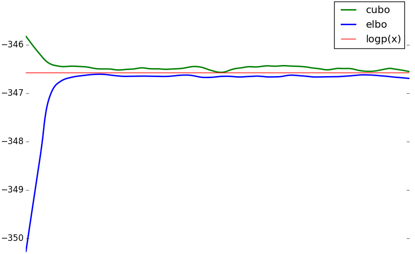
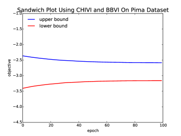
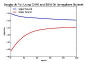
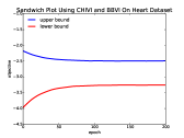
We analyze inference for Bayesian probit regression. First, we illustrate sandwich estimation on UCI datasets. Figure 1 illustrates the bounds of the log marginal likelihood given by the elbo and the cubo. Using both quantities provides a reliable approximation of the model evidence. In addition, these figures show convergence for chivi, which ep does not always satisfy.

We also compared the predictive performance of chivi, ep, and klvi. We used a minibatch size of $64$ and $2000$ iterations for each batch. We computed the average classification error rate and the standard deviation using $50$ random splits of the data. We split all the datasets with $90\%$ of the data for training and $10\%$ for testing. For the Covertype dataset, we implemented Bayesian probit regression to discriminate the class $1$ against all other classes. Table 1 shows the average error rate for klvi, ep, and chivi. chivi performs better for all but one dataset.

Figure 1: Sandwich gap via chivi and bbvi on different datasets. The first two plots correspond to sandwich plots for the two UCI datasets Ionosphere and Heart respectively. The last plot corresponds to a sandwich for generated data where we know the log marginal likelihood of the data. There the gap is tight after only few iterations. More sandwich plots can be found in the appendix.

Table 1: Test error for Bayesian probit regression. The lower the better. chivi (this paper) yields lower test error rates when compared to bbvi [12], and ep on most datasets.

Dataset	bbvi	ep	chivi
Pima	0.235 $\pm$ 0.006	0.234 $\pm$ 0.006	0.222 $\pm$ 0.048
Ionos	0.123 $\pm$ 0.008	0.124 $\pm$ 0.008	0.116 $\pm$ 0.05
Madelon	0.457 $\pm$ 0.005	0.445 $\pm$ 0.005	0.453 $\pm$ 0.029
Covertype	0.157 $\pm$ 0.01	0.155 $\pm$ 0.018	0.154 $\pm$ 0.014

3.2 Gaussian Process Classification

Table 2: Test error for Gaussian process classification. The lower the better. chivi (this paper) yields lower test error rates when compared to Laplace and ep on most datasets.

Dataset	Laplace	ep	chivi
Crabs	0.02	0.02	0.03 $\pm$ 0.03
Sonar	0.154	0.139	0.055 $\pm$ 0.035
Ionos	0.084	0.08 $\pm$ 0.04	0.069 $\pm$ 0.034

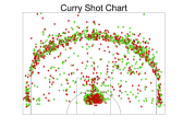
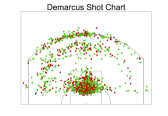
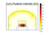
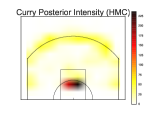
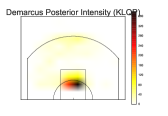
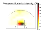
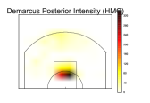
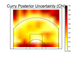
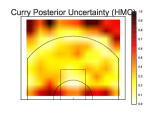
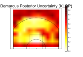
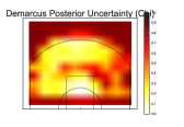
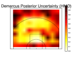
Figure 2: Basketball players shooting profiles as inferred by bbvi [12], chivi (this paper), and hmc. The top row displays the raw data, consisting of made shots (green) and missed shots (red). The second and third rows display the posterior intensities inferred by bbvi, chivi, and hmc for Stephen Curry and Demarcus Cousins respectively. Both bbvi and chivi capture the shooting behavior of both players in terms of the posterior mean. The last two rows display the posterior uncertainty inferred by bbvi, chivi, and hmc for Stephen Curry and Demarcus Cousins respectively. chivi tends to get higher posterior uncertainty for both players in areas where data is scarce compared to bbvi. This illustrates the variance underestimation problem of klvi, which is not the case for chivi. More player profiles with posterior mean and uncertainty estimates can be found in the appendix.

gp classification is an alternative to probit regression. The posterior is analytically intractable because the likelihood is not conjugate to the prior. Moreover, the posterior tends to be skewed. ep has been the method of choice for approximating the posterior [8]. We choose a factorized Gaussian for the variational distribution $q$ and fit its mean and $\log$ variance parameters.

With UCI benchmark datasets, we compared the predictive performance of chivi to ep and Laplace. Table 2 summarizes the results. The error rates for chivi correspond to the average of $10$ error rates obtained by dividing the data into $10$ folds, applying chivi to $9$ folds to learn the variational parameters and performing prediction on the remainder. The kernel hyperparameters were chosen using grid search. The error rates for the other methods correspond to the best results reported in [8] and [34]. On all the datasets chivi performs as well or better than ep and Laplace.

3.3 Cox Processes

Finally we study Cox processes. They are Poisson processes with stochastic rate functions. They capture dependence between the frequency of points in different regions of a space. We apply Cox processes to model the spatial locations of shots (made and missed) from the 2015-2016 NBA season [35]. The data are from $308$ NBA players who took more than $150,000$ shots in total. The $n^{th}$ player’s set of $M_{n}$ shot attempts are $\boldsymbol{\mathbf{x}}_{n}=\{\boldsymbol{\mathbf{x}}_{n,1},...,\boldsymbol{\mathbf{x}}_{n,M_{n}}\}$, and the location of the $m^{th}$ shot by the $n^{th}$ player in the basketball court is $\boldsymbol{\mathbf{x}}_{n,m}\in[-25,25]\times[0,40]$. Let $\mathcal{PP}(\boldsymbol{\mathbf{\lambda}})$ denote a Poisson process with intensity function $\boldsymbol{\mathbf{\lambda}}$, and $\boldsymbol{\mathbf{K}}$ be a covariance matrix resulting from a kernel applied to every location of the court. The generative process for the $n^{th}$ player’s shot is

$$\boldsymbol{\mathbf{K}}_{i,j} =k(\boldsymbol{\mathbf{x}}_{i},\boldsymbol{\mathbf{x}}_{j})=\sigma^{2}\exp(-\frac{1}{2\phi^{2}}||\boldsymbol{\mathbf{x}}_{i}-\boldsymbol{\mathbf{x}}_{j}||^{2})$$

f $$\sim\mathcal{GP}(0,k(\cdot,\cdot))\text{ ; }\boldsymbol{\mathbf{\lambda}}=\exp(\textbf{f})\text{ ; }\boldsymbol{\mathbf{x}}_{n,k}\sim\mathcal{PP}(\boldsymbol{\mathbf{\lambda}})\text{ for }k\in\{1,...,M_{n}\}.$$

The kernel of the Gaussian process encodes the spatial correlation between different areas of the basketball court. The model treats the $N$ players as independent. But the kernel $\boldsymbol{\mathbf{K}}$ introduces correlation between the shots attempted by a given player.

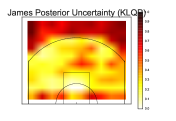
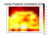
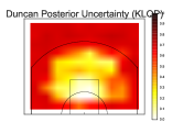
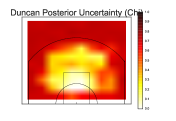
Our goal is to infer the intensity functions $\lambda(.)$ for each player. We compare the shooting profiles of different players using these inferred intensity surfaces. The results are shown in Figure 2. The shooting profiles of Demarcus Cousins and Stephen Curry are captured by both bbvi and chivi. bbvi has lower posterior uncertainty while chivi provides more overdispersed solutions. We plot the profiles for two more players, LeBron James and Tim Duncan, in the appendix.

Table 3: Average $L_{1}$ error for posterior uncertainty estimates (ground truth from hmc). We find that chivi is similar to or better than bbvi at capturing posterior uncertainties. Demarcus Cousins, who plays center, stands out in particular. His shots are concentrated near the basket, so the posterior is uncertain over a large part of the court Figure 2.

	Curry	Demarcus	Lebron	Duncan
chivi	0.060	0.073	0.0825	0.0849
bbvi	0.066	0.082	0.0812	0.0871

In Table 3, we compare the posterior uncertainty estimates of chivi and bbvi to that of hmc, a computationally expensive Markov chain Monte Carlo procedure that we treat as exact. We use the average $L_{1}$ distance from hmc as error measure. We do this on four different players: Stephen Curry, Demarcus Cousins, LeBron James, and Tim Duncan. We find that chivi is similar or better than bbvi, especially on players like Demarcus Cousins who shoot in a limited part of the court.

4 Discussion

We described chivi, a black box algorithm that minimizes the $\chi$-divergence by minimizing the cubo. We motivated chivi as a useful alternative to ep. We justified how the approach used in chivi enables upper bound minimization contrary to existing $\alpha$-divergence minimization techniques. This enables sandwich estimation using variational inference instead of Markov chain Monte Carlo. We illustrated this by showing how to use chivi in concert with klvi to sandwich-estimate the model evidence. Finally, we showed that chivi is an effective algorithm for Bayesian probit regression, Gaussian process classification, and Cox processes.

Performing vi via upper bound minimization, and hence enabling overdispersed posterior approximations, sandwich estimation, and model selection, comes with a cost. Exponentiating the original cubo bound leads to high variance during optimization even with reparameterization gradients. Developing variance reduction schemes for these types of objectives (expectations of likelihood ratios) is an open research problem; solutions will benefit this paper and related approaches.

Appendix A Proof of Sandwich Theorem

We denote by $\boldsymbol{\mathbf{z}}$ the latent variable and $\boldsymbol{\mathbf{x}}$ the data. Assume $\boldsymbol{\mathbf{z}}\in R^{D}$.

We first show that cubo _n is a nondecreasing function of the order $n$ of the $\chi$-divergence. Denote by the triplet $(\Omega,\mathcal{F},Q)$ the probability space induced by the variational distribution $q$ where $\Omega$ is a subspace of $R^{D}$, $\mathcal{F}$ is the corresponding Borel sigma algebra, and $Q$ is absolutely continuous with respect to the Lebesgue measure $\mu$ and is such that $dQ(\boldsymbol{\mathbf{z}})=q(\boldsymbol{\mathbf{z}})dz$. Define $w=\frac{p(\boldsymbol{\mathbf{x}},\boldsymbol{\mathbf{z}})}{q(\boldsymbol{\mathbf{z}})}$. We can rewrite $\lx@glossaries@gls@link{acronym}{CUBO}{\leavevmode\textsc{cubo}}_{n}$ as:

$$\lx@glossaries@gls@link{acronym}{CUBO}{\leavevmode\textsc{cubo}}_{n} =\frac{1}{n}\log E_{q}[w^{n}]=\log\Big{(}(E_{q}[w^{n}])^{\frac{1}{n}}\Big{)}$$

Since $\log$ is nondecreasing, it is enough to show
$n\mapsto(E_{q}[w^{n}])^{\frac{1}{n}}$ is nondecreasing. This function is the $L_{n}$ norm in the space defined above:

$$(E_{q}[w^{n}])^{\frac{1}{n}} =\Big{(}\int_{\Omega}|w|^{n}dQ\Big{)}^{\frac{1}{n}}=\Big{(}\int_{\Omega}|w|^{n}q(\boldsymbol{\mathbf{z}})d\boldsymbol{\mathbf{z}}\Big{)}^{\frac{1}{n}}$$

This is a nondecreasing function of $n$ by virtue of the Lyapunov inequality.

We now show the second claim in the sandwich theorem, namely that the limit when $n\rightarrow 0$ of $\lx@glossaries@gls@link{acronym}{CUBO}{\leavevmode\textsc{cubo}}_{n}$ is the elbo. Since $\lx@glossaries@gls@link{acronym}{CUBO}{\leavevmode\textsc{cubo}}_{n}$ is a monotonic function of $n$ and is bounded from below by elbo, it admits a limit when $n\rightarrow 0$. Call this limit $L$. We show $L=\lx@glossaries@gls@link{acronym}{ELBO}{\leavevmode\textsc{elbo}}$. On the one hand, since $\lx@glossaries@gls@link{acronym}{CUBO}{\leavevmode\textsc{cubo}}_{n}\geq\lx@glossaries@gls@link{acronym}{ELBO}{\leavevmode\textsc{elbo}}$ for all $n>0$, we have $L\geq\lx@glossaries@gls@link{acronym}{ELBO}{\leavevmode\textsc{elbo}}$. On the other hand, since $\log t\leq t-1$; $\forall t>0$ we have

$$\lx@glossaries@gls@link{acronym}{CUBO}{\leavevmode\textsc{cubo}}_{n} =\frac{1}{n}\log E_{q}[w^{n}]\leq\frac{1}{n}\Big{[}E_{q}[w^{n}]-1\Big{]}=E_{q}\Big{[}\frac{w^{n}-1}{n}\Big{]}$$

$f:n\mapsto w^{n}$ is differentiable and furthermore
$f^{\prime}(0)=\lim_{n\to 0}\Big{[}\frac{w^{n}-1}{n}\Big{]}=\log w$. Therefore $\exists n_{0}>0$ such that $|\frac{w^{n}-1}{n}-\log w|<1$ $\forall n<n_{0}$.
Since $||\frac{w^{n}-1}{n}|-\log w|<|\frac{w^{n}-1}{n}-\log w|$, we have
$|\frac{w^{n}-1}{n}|<1+\log w$ which is $E_{q}$-integrable. Therefore by Lebesgue’s dominated convergence theorem: $\lim_{n\to 0}E_{q}\Big{[}\frac{w^{n}-1}{n}\Big{]}=E_{q}\Big{[}\lim_{n\to 0}\frac{w^{n}-1}{n}\Big{]}=E_{q}[\log w]=\lx@glossaries@gls@link{acronym}{ELBO}{\leavevmode\textsc{elbo}}$. Since $\lx@glossaries@gls@link{acronym}{CUBO}{\leavevmode\textsc{cubo}}_{n}$ converges when $n\rightarrow 0$ and $\lx@glossaries@gls@link{acronym}{CUBO}{\leavevmode\textsc{cubo}}_{n}\leq E_{q}\Big{[}\frac{w^{n}-1}{n}\Big{]}$ $\forall n$, we establish $L\leq\lim_{n\to 0}E_{q}\Big{[}\frac{w^{n}-1}{n}\Big{]}=\lx@glossaries@gls@link{acronym}{ELBO}{\leavevmode\textsc{elbo}}$. The conclusion follows.

Appendix B The chivi algorithm for small datasets

In the main text we derived a subsampling version of chivi. For very small datasets, the average likelihood technique is not needed. The algorithm then uses all the data at each iteration and is summarized in Algorithm 2.

Input: Data $\boldsymbol{\mathbf{x}}$, Model $p(\boldsymbol{\mathbf{x}},\boldsymbol{\mathbf{z}})$, Variational family $q(\boldsymbol{\mathbf{z}};\boldsymbol{\mathbf{\lambda}})$.

Output: Variational parameters $\boldsymbol{\mathbf{\lambda}}$.

Initialize $\boldsymbol{\mathbf{\lambda}}$ randomly. while not converged do

       Draw $S$ samples $\boldsymbol{\mathbf{z}}^{(1)},...,\boldsymbol{\mathbf{z}}^{(S)}$ from $q(\boldsymbol{\mathbf{z}};\boldsymbol{\mathbf{\lambda}})$. Set $\rho_{t}$ from a Robbins-Monro sequence. Set $\log\boldsymbol{\mathbf{w}}^{(s)}=\log p(\boldsymbol{\mathbf{x}},\boldsymbol{\mathbf{z}}^{(s)})-\log q(\boldsymbol{\mathbf{z}}^{(s)};\boldsymbol{\mathbf{\lambda}}_{t})$, $s\in\{1,...,S\}$. Set $c=\displaystyle\max_{s}\log\boldsymbol{\mathbf{w}}^{(s)}$. Set $\boldsymbol{\mathbf{w}}^{(s)}=\exp(\log\boldsymbol{\mathbf{w}}^{(s)}-c),s\in\{1,...,S\}$. Update $\boldsymbol{\mathbf{\lambda}}_{t+1}=\boldsymbol{\mathbf{\lambda}}_{t}-\frac{(1-n)\cdot\rho_{t}}{S}\sum_{s=1}^{S}\Big{[}\Big{(}\boldsymbol{\mathbf{w}}^{(s)}\Big{)}^{n}\nabla_{\boldsymbol{\mathbf{\lambda}}}\log q(\boldsymbol{\mathbf{z}}^{(s)};\boldsymbol{\mathbf{\lambda}}_{t})\Big{]}$.

end while

Algorithm 2 chivi without average likelihoods

Appendix C Approximately minimizing an $f$-divergence with chivi

In this section we provide a proof that minimizing an $f$-divergence can be done by minimizing a sum of $\chi$-divergencesThese individual $\chi$-divergences can then be optimized via chivi. Consider

$$D_{f}(p\,\|\,q)=\int f\Big{(}\frac{p(x)}{q(x)}\Big{)}q(x)dx$$

Without loss of generality assume $f$ is analytic. The Taylor expansion of $f$ around a given point $x_{0}$ is

$$f(x)=f(x_{0})+f^{\prime}(x_{0})(x-x_{0})+\sum_{i=2}^{\infty}f^{(i)}(x_{0})\frac{(x-x_{0})^{i}}{i!}$$

Therefore

$$D_{f}(p\,\|\,q) =f(x_{0})+f^{\prime}(x_{0})\Big{(}\mathbb{E}_{q(\boldsymbol{\mathbf{z}}\,|\,\boldsymbol{\mathbf{\lambda}})}\Big{[}\frac{p(x)}{q(x)}\Big{]}-x_{0}\Big{)}+\mathbb{E}_{q(\boldsymbol{\mathbf{z}}\,|\,\boldsymbol{\mathbf{\lambda}})}\Big{[}\sum_{i=2}^{\infty}\frac{f^{(i)}(x_{0})}{i!}\Big{(}\frac{p(x)}{q(x)}-x_{0}\Big{)}^{i}\Big{]}$$

$$=f(x_{0})+f^{\prime}(x_{0})(1-x_{0})+\sum_{i=2}^{\infty}\frac{f^{(i)}(1)}{i!}\mathbb{E}_{q(\boldsymbol{\mathbf{z}}\,|\,\boldsymbol{\mathbf{\lambda}})}\Big{[}\Big{(}\frac{p(x)}{q(x)}-1\Big{)}^{i}\Big{]}$$

where we switch summation and expectation by invoking Fubini’s theorem. In particular if we take $x_{0}=1$ the linear terms are zero and we end up with:

$$D_{f}(p\,\|\,q) =\sum_{i=2}^{\infty}\frac{f^{(i)}(1)}{i!}\mathbb{E}_{q(\boldsymbol{\mathbf{z}}\,|\,\boldsymbol{\mathbf{\lambda}})}\Big{[}\Big{(}\frac{p(x)}{q(x)}-1\Big{)}^{i}\Big{]}=\sum_{i=2}^{\infty}\frac{f^{(i)}(1)}{i!}D_{\chi^{i}}(p\,\|\,q)$$

If $f$ is not analytic but $k$ times differentiable for some $k$ then the proof still holds considering the Taylor expansion of $f$ up to the order $k$.

Appendix D Importance sampling

In this section we establish the relationship between $\chi^{2}$-divergence minimization and importance sampling. Consider estimating the marginal likelihood $I$ with importance sampling:

$$I =p(\boldsymbol{\mathbf{x}})=\int p(\boldsymbol{\mathbf{x}},\boldsymbol{\mathbf{z}})d\boldsymbol{\mathbf{z}}=\int\frac{p(\boldsymbol{\mathbf{x}},\boldsymbol{\mathbf{z}})}{q(\boldsymbol{\mathbf{z}};\boldsymbol{\mathbf{\lambda}})}q(\boldsymbol{\mathbf{z}};\boldsymbol{\mathbf{\lambda}})d\boldsymbol{\mathbf{z}}=\int w(\boldsymbol{\mathbf{z}})q(\boldsymbol{\mathbf{z}};\boldsymbol{\mathbf{\lambda}})d\boldsymbol{\mathbf{z}}$$

The Monte Carlo estimate of $I$ is

$$\hat{I}=\frac{1}{B}\sum_{b=1}^{B}w(\boldsymbol{\mathbf{z}}^{(b)})$$

where $\boldsymbol{\mathbf{z}}^{(1)},...,\boldsymbol{\mathbf{z}}^{(B)}\sim q(\boldsymbol{\mathbf{z}};\boldsymbol{\mathbf{\lambda}})$. The variance of $\hat{I}$ is

$$\operatorname{Var}(\hat{I}) =\frac{1}{B}[\mathbb{E}_{q(\boldsymbol{\mathbf{z}};\boldsymbol{\mathbf{\lambda}})}(w(\boldsymbol{\mathbf{z}}^{(b)})^{2})-(\mathbb{E}_{q(\boldsymbol{\mathbf{z}};\boldsymbol{\mathbf{\lambda}})}(w(\boldsymbol{\mathbf{z}}^{(b)})))^{2}]=\frac{1}{B}\Big{[}\mathbb{E}_{q(\boldsymbol{\mathbf{z}};\boldsymbol{\mathbf{\lambda}})}\Big{(}\Big{(}\frac{p(\boldsymbol{\mathbf{x}},\boldsymbol{\mathbf{z}}^{(1)})}{q(\boldsymbol{\mathbf{z}}^{(1)};\boldsymbol{\mathbf{\lambda}})}\Big{)}^{2}\Big{)}-p(\boldsymbol{\mathbf{x}})^{2}\Big{]}$$

Therefore minimizing this variance is equivalent to minimizing the quantity

$$\mathbb{E}_{q(\boldsymbol{\mathbf{z}};\boldsymbol{\mathbf{\lambda}})}\Big{(}\Big{(}\frac{p(\boldsymbol{\mathbf{x}},\boldsymbol{\mathbf{z}}^{(1)})}{q(\boldsymbol{\mathbf{z}}^{(1)};\boldsymbol{\mathbf{\lambda}})}\Big{)}^{2}\Big{)}$$

which is equivalent to minimizing the $\chi^{2}$-divergence.

Appendix E General properties of the $\chi$-divergence

In this section we outline several properties of the $\chi$-divergence.

Conjugate symmetry  Define

$$f^{*}(u)=uf(\frac{1}{u})$$

to be the conjugate of $f$. $f^{*}$ is also convex and satisfies $f^{*}(1)=0$. Therefore $D_{f}^{*}(p\,\|\,q)$ is a valid divergence in the $f$-divergence family and:

$$D_{f}(q\,\|\,p) =\int f\Big{(}\frac{q(x)}{p(x)}\Big{)}p(x)dx=\int\frac{q(x)}{p(x)}f^{*}\Big{(}\frac{p(x)}{q(x)}\Big{)}p(x)dx=D_{f^{*}}(p\,\|\,q)$$

$D_{f}(q\,\|\,p)$ is symmetric if and only if $f=f^{*}$ which is not the case here. To symmetrize the divergence one can use

$$D(p\,\|\,q)=D_{f}(p\,\|\,q)+D_{f}^{*}(p\,\|\,q)$$

Invariance under parameter transformation.  Let $y=u(x)$ for some function $u$. Then by Jacobi $p(x)dx=p(y)dy$ and $q(x)dx=q(y)dy$.

$$D_{\chi^{n}}(p(x)\,\|\,q(x)) =\int_{x_{0}}^{x_{1}}\Big{(}\frac{p(x)}{q(x)}\Big{)}^{n}q(x)dx-1=\int_{y_{0}}^{y_{1}}\Big{(}\frac{p(y)\frac{dy}{dx}}{q(y)\frac{dy}{dx}}\Big{)}^{n}q(y)dy-1$$

$$=\int_{y_{0}}^{y_{1}}\Big{(}\frac{p(y)}{q(y)}\Big{)}^{n}q(y)dy-1=D_{\chi^{n}}(p(y)\,\|\,q(y))$$

Factorization for independent distributions.  Consider taking $p(x,y)=p_{1}(x)p_{2}(y)$ and $q(x,y)=q_{1}(x)q_{2}(y)$.

$$D_{\chi^{n}}(p(x,y)\,\|\,q(x,y)) =\int\frac{p(x,y)^{n}}{q(x,y)^{n-1}}dxdy=\int\frac{p_{1}(x)^{n}p_{2}(y)^{n}}{q_{1}(x)^{n-1}q_{2}(y)^{n-1}}dxdy$$

$$=\Big{(}\int\frac{p_{1}(x)^{n}}{q_{1}(x)^{n-1}}dx\Big{)}\cdot\Big{(}\int\frac{p_{2}(y)^{n}}{q_{2}(y)^{n-1}}dy\Big{)}$$

$$=D_{\chi^{n}}(p_{1}(x)\,\|\,q_{1}(x))\cdot D_{\chi^{n}}(p_{2}(y)\,\|\,q_{2}(y))$$

Therefore $\chi$-divergence is multiplicative under independent distributions while KL is additive.

Other properties.  The $\chi$-divergence enjoys some other properties that it shares with all members of the $f$-divergence family namely monotonicity with respect to the distributions and joint convexity.

Appendix F Derivation of the $\lx@glossaries@gls@link{acronym}{CUBO}{\leavevmode\textsc{cubo}}_{n}$

In this section we outline the derivation of $\lx@glossaries@gls@link{acronym}{CUBO}{\leavevmode\textsc{cubo}}_{n}$, the upper bound to the marginal likelihood induced by the minimization of the $\chi$-divergence.
By definition:

$$D_{\chi^{n}}(p(\boldsymbol{\mathbf{z}}\,|\,\boldsymbol{\mathbf{x}})\,\|\,q(\boldsymbol{\mathbf{z}};\boldsymbol{\mathbf{\lambda}})) =\mathbb{E}_{q(\boldsymbol{\mathbf{z}};\boldsymbol{\mathbf{\lambda}})}\Big{[}\Big{(}\frac{p(\boldsymbol{\mathbf{z}}|\boldsymbol{\mathbf{x}})}{q(\boldsymbol{\mathbf{z}};\boldsymbol{\mathbf{\lambda}})}\Big{)}^{n}-1\Big{]}$$

Following the derivation of elbo, we seek an expression of $\log(p(\boldsymbol{\mathbf{x}}))$ involving this divergence. We achieve that as follows:

$$\mathbb{E}_{q(\boldsymbol{\mathbf{z}};\boldsymbol{\mathbf{\lambda}})}\Big{[}\Big{(}\frac{p(\boldsymbol{\mathbf{z}}\,|\,\boldsymbol{\mathbf{x}})}{q(\boldsymbol{\mathbf{z}};\boldsymbol{\mathbf{\lambda}})}\Big{)}^{n}\Big{]} =1+D_{\chi^{n}}(p(\boldsymbol{\mathbf{z}}\,|\,\boldsymbol{\mathbf{x}})\,\|\,q(\boldsymbol{\mathbf{z}};\boldsymbol{\mathbf{\lambda}}))\mathbb{E}_{q(\boldsymbol{\mathbf{z}};\boldsymbol{\mathbf{\lambda}})}\Big{[}\Big{(}\frac{p(\boldsymbol{\mathbf{x}},\boldsymbol{\mathbf{z}})}{q(\boldsymbol{\mathbf{z}};\boldsymbol{\mathbf{\lambda}})}\Big{)}^{n}\Big{]}$$

$$=p(\boldsymbol{\mathbf{x}})^{n}[1+D_{\chi^{n}}(p(\boldsymbol{\mathbf{z}}\,|\,\boldsymbol{\mathbf{x}})\,\|\,q(\boldsymbol{\mathbf{z}};\boldsymbol{\mathbf{\lambda}}))]$$

This gives the relationship

$$\log p(\boldsymbol{\mathbf{x}}) =\frac{1}{n}\log\mathbb{E}_{q(\boldsymbol{\mathbf{z}};\boldsymbol{\mathbf{\lambda}})}\Big{[}\Big{(}\frac{p(\boldsymbol{\mathbf{x}},\boldsymbol{\mathbf{z}})}{q(\boldsymbol{\mathbf{z}};\boldsymbol{\mathbf{\lambda}})}\Big{)}^{n}\Big{]}-\frac{1}{n}\log(1+D_{\chi^{n}}(p(\boldsymbol{\mathbf{z}}\,|\,\boldsymbol{\mathbf{x}})\,\|\,q(\boldsymbol{\mathbf{z}};\boldsymbol{\mathbf{\lambda}})))$$

$$\log p(\boldsymbol{\mathbf{x}}) =\lx@glossaries@gls@link{acronym}{CUBO}{\leavevmode\textsc{cubo}}_{n}-\frac{1}{n}\log(1+D_{\chi^{n}}(p(\boldsymbol{\mathbf{z}}|\boldsymbol{\mathbf{x}})\,\|\,q(\boldsymbol{\mathbf{z}};\boldsymbol{\mathbf{\lambda}})))$$

By nonnegativity of the divergence this last equation establishes the upper bound:

$$\log p(\boldsymbol{\mathbf{x}})\leq\lx@glossaries@gls@link{acronym}{CUBO}{\leavevmode\textsc{cubo}}_{n}$$

Appendix G Black Box Inference

In this section we derive the score gradient and the reparameterization gradient for doing black box inference with the $\chi$-divergence.

$$\lx@glossaries@gls@link{acronym}{CUBO}{\leavevmode\textsc{cubo}}_{n}(\boldsymbol{\mathbf{\lambda}})=\frac{1}{n}\log\mathbb{E}_{q(\boldsymbol{\mathbf{z}};\boldsymbol{\mathbf{\lambda}})}\Big{[}\Big{(}\frac{p(\boldsymbol{\mathbf{x}},\boldsymbol{\mathbf{z}})}{q(\boldsymbol{\mathbf{z}};\boldsymbol{\mathbf{\lambda}})}\Big{)}^{n}\Big{]}$$

where $\boldsymbol{\mathbf{\lambda}}$ is the set of variational parameters. To minimize $\lx@glossaries@gls@link{acronym}{CUBO}{\leavevmode\textsc{cubo}}_{n}(\boldsymbol{\mathbf{\lambda}})$ with respect to $\boldsymbol{\mathbf{\lambda}}$ we need to resort to Monte Carlo. To minimize $\lx@glossaries@gls@link{acronym}{CUBO}{\leavevmode\textsc{cubo}}_{n}(\boldsymbol{\mathbf{\lambda}})$ we consider the equivalent minimization of $\exp\{n\cdot\lx@glossaries@gls@link{acronym}{CUBO}{\leavevmode\textsc{cubo}}(\boldsymbol{\mathbf{\lambda}})\}$. This enables unbiased estimation of the noisy gradient used to perform black box inference with the $\chi$-divergence.

The score gradient  The score gradient of our objective function

$$\boldsymbol{\mathbf{L}}=\exp\{n\cdot\lx@glossaries@gls@link{acronym}{CUBO}{\leavevmode\textsc{cubo}}(\boldsymbol{\mathbf{\lambda}})\}$$

is derived below:

$$\nabla_{\boldsymbol{\mathbf{\lambda}}}\boldsymbol{\mathbf{L}} =\nabla_{\boldsymbol{\mathbf{\lambda}}}\int p(\boldsymbol{\mathbf{x}},\boldsymbol{\mathbf{z}})^{n}q(\boldsymbol{\mathbf{z}};\boldsymbol{\mathbf{\lambda}})^{1-n}d\boldsymbol{\mathbf{z}}=\int p(\boldsymbol{\mathbf{x}},\boldsymbol{\mathbf{z}})^{n}\nabla_{\boldsymbol{\mathbf{\lambda}}}q(\boldsymbol{\mathbf{z}};\boldsymbol{\mathbf{\lambda}})^{1-n}d\boldsymbol{\mathbf{z}}$$

$$=\int p(\boldsymbol{\mathbf{x}},\boldsymbol{\mathbf{z}})^{n}(1-n)q(\boldsymbol{\mathbf{z}};\boldsymbol{\mathbf{\lambda}})^{-n}\nabla_{\boldsymbol{\mathbf{\lambda}}}q(\boldsymbol{\mathbf{z}};\boldsymbol{\mathbf{\lambda}})d\boldsymbol{\mathbf{z}}=(1-n)\int(\frac{p(\boldsymbol{\mathbf{x}},\boldsymbol{\mathbf{z}})}{q(\boldsymbol{\mathbf{z}};\boldsymbol{\mathbf{\lambda}})})^{n}\nabla_{\boldsymbol{\mathbf{\lambda}}}q(\boldsymbol{\mathbf{z}};\boldsymbol{\mathbf{\lambda}})d\boldsymbol{\mathbf{z}}$$

$$=(1-n)\int(\frac{p(\boldsymbol{\mathbf{x}},\boldsymbol{\mathbf{z}})}{q(\boldsymbol{\mathbf{z}};\boldsymbol{\mathbf{\lambda}})})^{n}\nabla_{\boldsymbol{\mathbf{\lambda}}}\log q(\boldsymbol{\mathbf{z}};\boldsymbol{\mathbf{\lambda}})q(\boldsymbol{\mathbf{z}};\boldsymbol{\mathbf{\lambda}})d\boldsymbol{\mathbf{z}}=(1-n)\mathbb{E}_{q(\boldsymbol{\mathbf{z}};\boldsymbol{\mathbf{\lambda}})}\Big{[}\Big{(}\frac{p(\boldsymbol{\mathbf{x}},\boldsymbol{\mathbf{z}})}{q(\boldsymbol{\mathbf{z}};\boldsymbol{\mathbf{\lambda}})}\Big{)}^{n}\nabla_{\boldsymbol{\mathbf{\lambda}}}\log q(\boldsymbol{\mathbf{z}};\boldsymbol{\mathbf{\lambda}})\Big{]}$$

where we switched differentiation and integration by invoking Lebesgue’s dominated convergence theorem. We estimate this gradient with the unbiased estimator:

$$\frac{(1-n)}{B}\sum_{b=1}^{B}\Big{[}\Big{(}\frac{p(\boldsymbol{\mathbf{x}},\boldsymbol{\mathbf{z}}^{(b)})}{q(\boldsymbol{\mathbf{z}}^{(b)};\boldsymbol{\mathbf{\lambda}})}\Big{)}^{n}\nabla_{\boldsymbol{\mathbf{\lambda}}}\log q(\boldsymbol{\mathbf{z}}^{(b)};\boldsymbol{\mathbf{\lambda}})\Big{]}$$

Reparameterization gradient  The reparameterization gradient empirically has lower variance than the score gradient. We used it in our experiments. Denote by $L$ the quantity $\exp\{n\cdot\lx@glossaries@gls@link{acronym}{CUBO}{\leavevmode\textsc{cubo}}\}$. Assume $\boldsymbol{\mathbf{z}}=g(\boldsymbol{\mathbf{\lambda}},\epsilon)$ where $\epsilon\sim p(\epsilon)$. Then

$$\hat{L}=\frac{1}{B}\sum_{b=1}^{B}\Big{(}\frac{p(\boldsymbol{\mathbf{x}},g(\boldsymbol{\mathbf{\lambda}},\epsilon^{(b)}))}{q(g(\boldsymbol{\mathbf{\lambda}},\epsilon^{(b)});\boldsymbol{\mathbf{\lambda}})}\Big{)}^{n}$$

is an unbiased estimator of $L$ and its gradient is given by

$$\nabla_{\boldsymbol{\mathbf{\lambda}}}\hat{L} =\frac{n}{B}\sum_{b=1}^{B}\Big{(}\frac{p(\boldsymbol{\mathbf{x}},g(\boldsymbol{\mathbf{\lambda}},\epsilon^{(b)}))}{q(g(\boldsymbol{\mathbf{\lambda}},\epsilon^{(b)});\boldsymbol{\mathbf{\lambda}})}\Big{)}^{n}\nabla_{\boldsymbol{\mathbf{\lambda}}}\log\Big{(}\frac{p(\boldsymbol{\mathbf{x}},g(\boldsymbol{\mathbf{\lambda}},\epsilon^{(b)}))}{q(g(\boldsymbol{\mathbf{\lambda}},\epsilon^{(b)});\boldsymbol{\mathbf{\lambda}})}\Big{)}.$$

Appendix H More illustrations

The following figures are results of various experimentations with the cubo.

Figure 3:

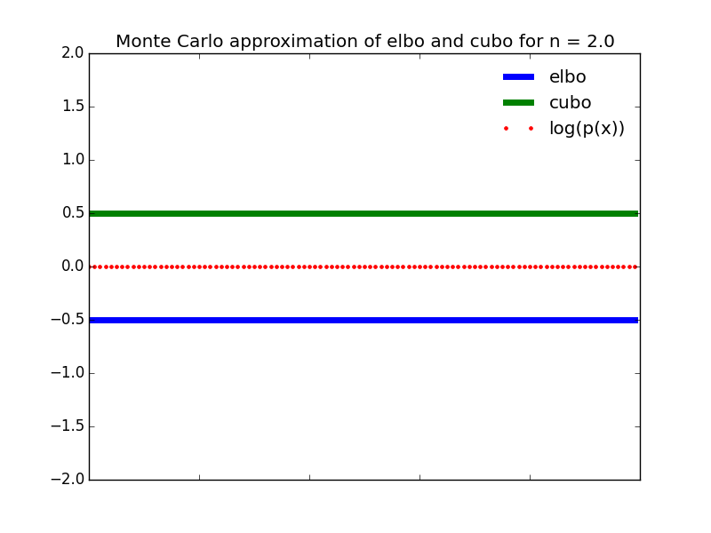
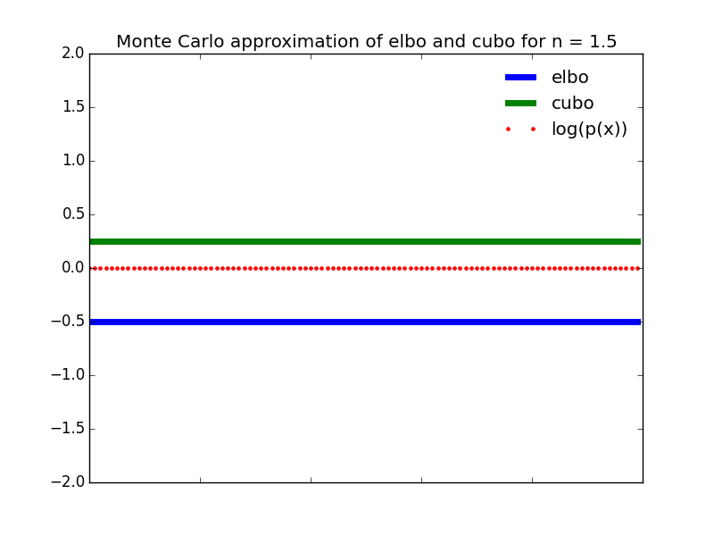
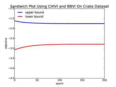
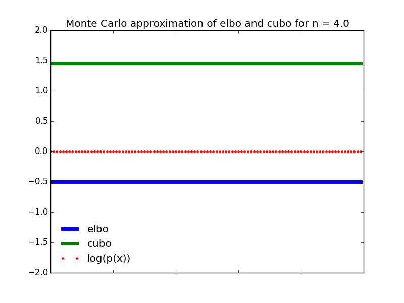
Figure 4: More sandwich plots via chivi and bbvi. The first three plots show simulated sandwich gaps when the order of the $\chi$-divergence is $n=4$, $n=2$, and $n=1.5$ respectively. As we demonstrated theoretically, the gap closes as $n$ decreases. The fourth plot is a sandwich on synthetic data where we know the log marginal likelihood of the data. Here the gap tightens after only $100$ iterations. The final two plots are sandwiches on real UCI datasets.

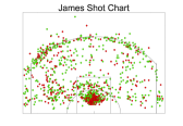
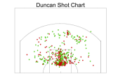
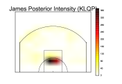
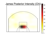
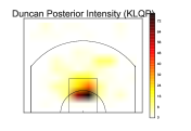
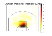
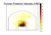
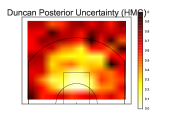
Figure 5: More player profiles. Basketball players shooting profiles as inferred by bbvi [12], chivi (this paper) and hmc. The top row displays the raw data, consisting of made shots (green) and missed shots (red). The second and third rows display the posterior intensities inferred by bbvi, chivi and hmc for Lebron James and Tim Duncan respectively. Both bbvi and chivi nicely capture the shooting behavior of both players in terms of their posterior mean.The fourth and fifth rows display the posterior uncertainty inferred by bbvi, chivi and hmc for Lebron James and Tim Duncan respectively. Here chivi and bbvi tend to get similar posterior uncertainty for Lebron James. chivi has better uncertainty for Tim Duncan.

References

• [1] C.Β Robert and G.Β Casella. Monte Carlo Statistical Methods. Springer-Verlag, 2004.
• [2] M.Β Jordan, Z.Β Ghahramani, T.Β Jaakkola, and L.Β Saul. Introduction to variational methods for graphical models. Machine Learning, 37:183–233, 1999.
• [3] M.Β D. Hoffman, D.Β M. Blei, C.Β Wang, and J.Β Paisley. Stochastic variational inference. JMLR, 2013.
• [4] K.Β P. Murphy. Machine Learning: A Probabilistic Perspective. MIT press, 2012.
• [5] C.Β M. Bishop. Pattern recognition. Machine Learning, 128, 2006.
• [6] J.Β Hensman, M.Β Zwießele, and N.Β D. Lawrence. Tilted variational Bayes. JMLR, 2014.
• [7] T.Β Minka. A family of algorithms for approximate Bayesian inference. PhD thesis, MIT, 2001.
• [8] M.Β Kuss and C.Β E. Rasmussen. Assessing approximate inference for binary Gaussian process classification. JMLR, 6:1679–1704, 2005.
• [9] M.Β J. Beal. Variational algorithms for approximate Bayesian inference. University of London, 2003.
• [10] D.Β J.Β C. MacKay. Bayesian interpolation. Neural Computation, 4(3):415–447, 1992.
• [11] R.Β B. Grosse, Z.Β Ghahramani, and R.Β P. Adams. Sandwiching the marginal likelihood using bidirectional monte carlo. arXiv preprint arXiv:1511.02543, 2015.
• [12] R.Β Ranganath, S.Β Gerrish, and D.Β M. Blei. Black box variational inference. In AISTATS, 2014.
• [13] D.Β P. Kingma and M.Β Welling. Auto-encoding variational Bayes. In ICLR, 2014.
• [14] D.Β J. Rezende, S.Β Mohamed, and D.Β Wierstra. Stochastic Backpropagation and Approximate Inference in Deep Generative Models. In ICML, 2014.
• [15] M.Β Opper and O.Β Winther. Gaussian processes for classification: Mean-field algorithms. Neural Computation, 12(11):2655–2684, 2000.
• [16] Andrew Gelman, Aki Vehtari, Pasi JylΓ€nki, Tuomas Sivula, Dustin Tran, Swupnil Sahai, Paul Blomstedt, JohnΒ P Cunningham, David Schiminovich, and Christian Robert. Expectation propagation as a way of life: A framework for Bayesian inference on partitioned data. arXiv preprint arXiv:1412.4869, 2017.
• [17] Y.Β W. Teh, L.Β Hasenclever, T.Β Lienart, S.Β Vollmer, S.Β Webb, B.Β Lakshminarayanan, and C.Β Blundell. Distributed Bayesian learning with stochastic natural-gradient expectation propagation and the posterior server. arXiv preprint arXiv:1512.09327, 2015.
• [18] Y.Β Li, J.Β M. HernΓ‘ndez-Lobato, and R.Β E. Turner. Stochastic Expectation Propagation. In NIPS, 2015.
• [19] T.Β Minka. Power EP. Technical report, Microsoft Research, 2004.
• [20] J.Β M. HernΓ‘ndez-Lobato, Y.Β Li, D.Β HernΓ‘ndez-Lobato, T.Β Bui, and R.Β E. Turner. Black-box α𝛼\alpha-divergence minimization. ICML, 2016.
• [21] Y.Β Li and R.Β E. Turner. Variational inference with RΓ©nyi divergence. In NIPS, 2016.
• [22] Rajesh Ranganath, Jaan Altosaar, Dustin Tran, and DavidΒ M. Blei. Operator variational inference. In NIPS, 2016.
• [23] Volodymyr Kuleshov and Stefano Ermon. Neural variational inference and learning in undirected graphical models. In NIPS, 2017.
• [24] M.Β I. Jordan, Z.Β Ghahramani, T.Β S. Jaakkola, and L.Β K. Saul. An introduction to variational methods for graphical models. Machine Learning, 37(2):183–233, 1999.
• [25] T.Β Minka. Divergence measures and message passing. Technical report, Microsoft Research, 2005.
• [26] Yuri Burda, Roger Grosse, and Ruslan Salakhutdinov. Importance Weighted Autoencoders. In International Conference on Learning Representations, 2016.
• [27] MatthewΒ D Hoffman. Learning Deep Latent Gaussian Models with Markov Chain Monte Carlo. In International Conference on Machine Learning, 2017.
• [28] D.Β J.Β C. MacKay. Information Theory, Inference, and Learning Algorithms. Cambridge Univ. Press, 2003.
• [29] A.Β E. Raftery. Bayesian model selection in social research. Sociological methodology, 25:111–164, 1995.
• [30] J.Β Paisley, D.Β Blei, and M.Β Jordan. Variational Bayesian inference with stochastic search. In ICML, 2012.
• [31] G.Β Dehaene and S.Β BarthelmΓ©. Expectation propagation in the large-data limit. In NIPS, 2015.
• [32] Peter Sunehag, Jochen Trumpf, SVN Vishwanathan, NicolΒ N Schraudolph, etΒ al. Variable metric stochastic approximation theory. In AISTATS, pages 560–566, 2009.
• [33] Dustin Tran, Alp Kucukelbir, AdjiΒ B Dieng, Maja Rudolph, Dawen Liang, and DavidΒ M Blei. Edward: A library for probabilistic modeling, inference, and criticism. arXiv preprint arXiv:1610.09787, 2016.
• [34] H.Β Kim and Z.Β Ghahramani. The em-ep algorithm for gaussian process classification. In Proceedings of the Workshop on Probabilistic Graphical Models for Classification (ECML), pages 37–48, 2003.
• [35] A.Β Miller, L.Β Bornn, R.Β Adams, and K.Β Goldsberry. Factorized point process intensities: A spatial analysis of professional basketball. In ICML, 2014.