Submodular Maximization over Sliding Windows

Abstract

In this paper we study the extraction of representative elements in the data stream model in the form of submodular maximization. Different from the previous work on streaming submodular maximization, we are interested only in the recent data, and study the maximization problem over sliding windows. We provide a general reduction from the sliding window model to the standard streaming model, and thus our approach works for general constraints as long as there is a corresponding streaming algorithm in the standard streaming model. As a consequence, we obtain the first algorithms in the sliding window model for maximizing a monotone/non-monotone submodular function under cardinality and matroid constraints. We also propose several heuristics and show their efficiency in real-world datasets.

1 Introduction

The last few decades have witnessed an explosion in the amount of data involved in machine learning tasks. In many cases, the data volume exceeds our storage capacity and demands new techniques that can effectively learn while operating within stringent storage and computation limits. Streaming algorithms [15] have emerged as a powerful approach to cope with massive data volume. In this model, the learning algorithm processes the dataset one element at a time by a linear scan and keeps only a small summary of the dataset in the memory; it is then able to compute the objective function on the processed elements using the summary. Various popular techniques in machine learning operate in this model, such as stochastic gradient descent, perceptron, etc. This model is particularly useful when the dataset is too large to fit in the memory or if the data is generated in real time (e.g., in online learning).

A common issue in online learning/streaming data mining is that the underlying distribution that generates the data may change over time. Therefore we had better consider only the most recently data in the stream. Streaming algorithms over sliding windows have already been designed for several problems, including $k$-median clustering [3], kernel least square regression [21], $k$-means and coreset construction [6], etc.

The window size can again be very large and does not fit the main memory. The problem becomes more severe in the case when kernel method is applied to deal with the nonlinear system – the resulting kernel matrix may need $O(W^{2})$ memory where $W$ is the window size. A natural idea to resolve this issue is to select representative data items from the window for computing the objective function.

Submodular functions, an abstract and broad class of functions, have recently become an attractive candidate for modeling a variety of scenarios in machine learning, from exemplar-based clustering [12], summarization [20] to determinantal point processes [11]. In recent years there have been quite some work on designing streaming algorithm for optimizing submodular functions [12, 13, 4, 8, 9]. However, we are not aware of any previous work dealing with streaming data over sliding windows in the context of submodular optimization.

In this work, we present a general reduction from the sliding window model to the standard streaming model. As a consequence, we immediately obtain algorithms in the sliding window model by combining with previous works in the standard streaming model for cardinality constraints [12, 13, 4], matroid and matching constraints [8], and non-monotone functions [9]. We also propose a few heuristics and compare their performance on real-world datasets.

2 Preliminaries

Let $V$ be the finite ground set (possibly multiset). Let $f:2^{V}\rightarrow\mathbb{R}$ be a function mapping subsets of $V$ to numbers. We say $f$ is submodular if $f(A\cup\{v\})-f(A)\geq f(B\cup\{v\})-f(B)$ for any $A\subseteq B\subset V$, and $v\in V\backslash B$. We define $f(v|A)=f(A\cup\{v\})-f(A)$ as the marginal gain of $v$ given $A$. If further we have $f(A)\leq f(B)$ for any $A\subseteq B\subseteq V$, we say $f$ is monotone.

In the general form of constrained submodular maximization problem, we consider solving

$$\operatorname*{argmax}_{S\in\mathcal{I}}f(S),$$ (1)

where $\mathcal{I}$ is a collection of subsets of $V$ which we call the constraint. In particular, when $\mathcal{I}=\{S\subseteq V~{}|~{}|S|\leq k\}$, Expression (1) is known as the cardinality constrained submodular maximization problem. Definitions for other constraints can be found in e.g. [5]. We say constraint $\mathcal{I}$ hereditary if $A\in\mathcal{I}$ implies that any subset of $A$ is also in $\mathcal{I}$.

For a constrained submodular maximization problem, we use $\mathtt{OPT}$ to represent the solution of (1). W.l.o.g. we assume $1\leq f(\mathtt{OPT})\leq M$ for a parameter $M$.

In the streaming model, we consider the ground set $V$ as an ordered sequence of items $e_{1},e_{2},\ldots,e_{n}$, each consumes one word of space. Each index is called a time step. In the sliding window model, we specify the window size $W$. At any time step, we are only interested in the most recent $W$ items which defines the ground set $V$ at that moment. Note that when $W\rightarrow\infty$, $V$ becomes the set of all received items; we thus also call the standard streaming model the infinite window model. For two streams/sequences $S_{1}$ and $S_{2}$, let $S_{1}\circ S_{2}$ be their concatenation, which is $S_{1}$ followed by $S_{2}$.

Let $\mathcal{A}$ be an algorithm solving the constrained submodular maximization problem. We use $\mathcal{A}(V)$ to represent the function value of the solution returned by $\mathcal{A}$ operating on the ground set $V$.

3 Algorithms

3.1 A Reduction to the Infinite Window Case

In this section we design sliding window algorithms by a generic reduction to standard infinite window streaming algorithms. Our reduction can work with any standard streaming algorithms that satisfy some natural properties. Throughout this section, we assume that the constraint in the submodular maximization problem is hereditary (see the preliminaries for definition).

Definition 1

Let $\mathcal{A}$ be an algorithm operating on a stream of elements, and $\mathcal{A}(S)$ be the value of the solution found by $\mathcal{A}$ on the stream $S$. We say $\mathcal{A}$ is $c$-compliant if it satisfies the following conditions:

• (Monotonicity) If $S_{1}$ is a prefix of $S_{2}$ then $\mathcal{A}(S_{1})\leq\mathcal{A}(S_{2})$.

• ($c$-Approximation) For any stream $S$, let $\mathtt{OPT}$ be the optimal solution. Then $\mathcal{A}(S)\geq c\cdot f(\mathtt{OPT})$.

The following lemma is similar to the smooth histogram technique introduced in [7]. However, smooth histogram only works for problems with good approximations. More precisely, it is assumed that there is an algorithm with $(1-\epsilon)$ approximation where $\epsilon<1/4$, which does not hold for many submodular problems. Our algorithm (Algorithm 1) also works for streaming algorithms without the monotonicity property, though monotonicity allows us to get a better approximation. Any streaming algorithm can be modified to satisfy the monotonicity property at the cost of increased update time: after every update, the algorithm calculates a solution and it keeps track of the best solution over time.

Lemma 1

Let stream $S_{1}\circ S_{2}\circ S_{3}$ be the concatenation of three (sub)streams $S_{1},S_{2},S_{3}$. Given a $c$-compliant algorithm $\mathcal{A}$, if $\mathcal{A}(S_{1}\circ S_{2})\leq(1+\epsilon)\mathcal{A}(S_{2})$, then $\mathcal{A}(S_{2}\circ S_{3})\geq\frac{c}{2+\epsilon}\cdot f(\mathtt{OPT}_{123})$ where $\mathtt{OPT}_{123}$ is the optimal solution for the stream $S_{1}\circ S_{2}\circ S_{3}$.

Proof.

Let $\mathtt{OPT}_{123},\mathtt{OPT}_{23},\mathtt{OPT}_{12}$ be the optimal solution for the streams $S_{1}\circ S_{2}\circ S_{3},S_{2}\circ S_{3},S_{1}\circ S_{2}$, respectively. We have

$$\textstyle\frac{1}{c}\cdot\mathcal{A}(S_{2}\circ S_{3})\geq f(\mathtt{OPT}_{23}).$$ (2)

We also have

$$\textstyle f(\mathtt{OPT}_{12})\leq\frac{1}{c}\cdot\mathcal{A}(S_{1}\circ S_{2})\leq\frac{1+\epsilon}{c}\cdot\mathcal{A}(S_{2})\leq\frac{1+\epsilon}{c}\cdot\mathcal{A}(S_{2}\circ S_{3}).$$ (3)

Combining (2) and (3), we obtain

$$\textstyle\frac{2+\epsilon}{c}\cdot\mathcal{A}(S_{2}\circ S_{3}) \geq f(\mathtt{OPT}_{12})+f(\mathtt{OPT}_{23})$$

$$\geq f(\mathtt{OPT}_{123}\cap S_{1})$$

$$+f(\mathtt{OPT}_{123}\cap(S_{2}\circ S_{3}))$$

$$\geq f(\mathtt{OPT}_{123}).$$

∎

We can also show a similar lemma for algorithms satisfying the $c$-approximation property but not monotonicity.

Lemma 2

Let stream $S_{1}\circ S_{2}\circ S_{3}$ be the concatenation of three (sub)streams $S_{1},S_{2},S_{3}$. Given an algorithm $\mathcal{A}$ with $c$-approximation property, if $\mathcal{A}(S_{1}\circ S_{2})\leq(1+\epsilon)\mathcal{A}(S_{2})$, then $\mathcal{A}(S_{2}\circ S_{3})\geq\frac{c^{2}}{c+1+\epsilon}\cdot f(\mathtt{OPT}_{123})$ where $\mathtt{OPT}_{123}$ is the optimal solution for the stream $S_{1}\circ S_{2}\circ S_{3}$.

The proof is similar to that of Lemma 2. The major modification is to use the following inequality, which does not require the monotonicity property, as a replacement of (3),

$$f(\mathtt{OPT}_{12}) \leq \frac{1}{c}\cdot\mathcal{A}(S_{1}\circ S_{2})\leq\frac{1+\epsilon}{c}\cdot\mathcal{A}(S_{2})$$

$$\leq \frac{(1+\epsilon)}{c}f(\mathtt{OPT}_{23})\leq\frac{1+\epsilon}{c^{2}}\mathcal{A}(S_{2}\circ S_{3}).$$

We have the following theorem.

Theorem 1

There is an algorithm for constrained submodular maximization over sliding windows that achieves a $c/(2+\epsilon)$-approximation using $O(s/\epsilon\cdot\log M)$ space and $O(t/\epsilon\cdot\log M)$ update time per item, provided that there is a corresponding $c$-compliant streaming algorithm using $s$ space and $t$ update time per item.

Input: $M$: an upper bound of $f(\mathtt{OPT})$ over sliding windows. $W$: the size of the window. $\mathcal{A}$ is an infinite window streaming algorithm which we use as a blackbox.

1 foreach new incoming element $e_{i}$ do

2       start a new instance $\mathcal{A}^{(i)}$

3       drop all maintained instances $\mathcal{A}^{(y)}$ where $y\leq i-W$

4       update all the remaining instances, denoted by $\mathcal{A}^{(t_{1})},\ldots,\mathcal{A}^{(t_{u})}$, with $e_{i}$

5       $j\leftarrow 1$

6       while $j<u$ do

7             $x\leftarrow u$

8             while  $(1+\epsilon)\mathcal{A}^{(t_{x})}(e_{t_{x}},\ldots,e_{i})<\mathcal{A}^{(t_{j})}(e_{t_{j}},\ldots,e_{i})$ do

9                   $x\leftarrow x-1$

10            Prune all $\mathcal{A}^{(t_{v})}$ with $j<v<x$

11             if $x\leq j$ then

12                   $x\leftarrow j+1$

13            $j\leftarrow x$

14      

return (at query) $\mathcal{A}^{(t_{b})}(e_{t_{b}},\ldots,e_{\mathtt{now}})$ where $t_{b}=\min\{t_{j}\in[\mathtt{now}-W+1,\mathtt{now}]\ |\ \mathcal{A}^{(t_{j})}\text{ is maintained}\}$

Algorithm 1 SW-RD$(\mathcal{A},W,M)$: A Reduction to Infinite Window Streaming Algorithms

The pseudocode of the algorithm is described in Algorithm 1. We now explain it in words. The algorithm maintains a collection of instances of $\mathcal{A}$ starting at different times $t_{1}<t_{2}<\ldots<t_{u}$, which we will denote by $\mathcal{A}^{(t_{1})},\mathcal{A}^{(t_{2})},\ldots,\mathcal{A}^{(t_{u})}$. Upon receiving a new element $e_{i}$, we perform the following operations. We first create a new instance $\mathcal{A}^{(i)}$. Next, we drop those instances of $\mathcal{A}$ that are expired, and update all the remaining instances with the new element $e_{i}$. Finally we perform a pruning procedure: We start with $t_{1}$. Let $t_{x}$ be the maximum time step among all the maintained instances of $\mathcal{A}$ such that $(1+\epsilon)\mathcal{A}^{(t_{x})}\geq\mathcal{A}^{(t_{1})}$. We prune all the instances $\mathcal{A}^{(t_{v})}$ where $1<v<x$ (Line 1-1). We repeat this pruning procedure with (the next unpruned time step) $t_{x}$ and continue until we reach $t_{u}$. Note that the purpose of the pruning step is to make the remaining data stream satisfy $\mathcal{A}(S_{1}\circ S_{2})\leq(1+\epsilon)\mathcal{A}(S_{2})$, so that Lemma 1 or Lemma 2 applies.

The space usage of the algorithm is again easy to bound. Note that after the pruning (we rename the remaining instances as $\mathcal{A}^{t_{1}},\mathcal{A}^{t_{2}},\ldots,\mathcal{A}^{t_{u}}$), for each $j=1,\ldots,u-2$, we have $\mathcal{A}^{(t_{j})}>(1+\epsilon)\mathcal{A}^{(t_{j+2})}$. Thus the number of instances of $\mathcal{A}$ is bounded by $O(1/\epsilon\cdot\log M)$ at all time steps. When doing the pruning, we only need to calculate the value of each instance once, so the processing time per item is $O(t/\epsilon\cdot\log M)$.

We next give the proof of the correctness. Let us consider a window $[i-W+1,i]$, and let $t_{b}=\min\{t_{j}\in[i-W+1,i]\ |\ j=1,\ldots,u\}$. For this window we will report whatever $\mathcal{A}^{(t_{b})}$ reports. It is easy to see that if $t_{b}=i-W+1$, then the algorithm is obviously correct since $\mathcal{A}^{(t_{b})}$ is a streaming algorithm starting from time $t_{b}$. We next consider the case when $t_{b}>i-W+1$. Let $t_{c}$ be the time step when the last $\mathcal{A}^{(t)}$ in $\{\mathcal{A}^{(i-W+1)}\ldots,\mathcal{A}^{(t_{b}-1)}\}$ was pruned, and let $t_{a}<i-W+1$ be the largest time step before $i-W+1$ such that $\mathcal{A}^{(t_{a})}$ is active after the pruning step at time $t_{c}$. Note that $t_{a}$ must exist because pruning always happens between two active instances (at Line 9 of the algorithm, we prune between $j$ and $x$ exclusively). It is clear that $t_{a}<t_{b}\leq t_{c}$. Let $S_{1}=(e_{t_{a}},\ldots,e_{t_{b}-1})$, $S_{2}=(e_{t_{b}},\ldots,e_{t_{c}})$, and $S_{3}=(e_{t_{c}+1},\ldots,e_{i})$. By the pruning rule, we have $(1+\epsilon)\mathcal{A}(S_{2})\geq\mathcal{A}(S_{1}\circ S_{2})$. Plugging in Lemma 1, we have

$$\textstyle\mathcal{A}(S_{2}\circ S_{3})\geq\frac{c}{2+\epsilon}\cdot f(\mathtt{OPT}_{123}),$$ (4)

where $\mathtt{OPT}_{123}$ is the optimal solution for the stream $S_{1}\circ S_{2}\circ S_{3}$, which includes the window $[i-W+1,i]$.

In [4] the authors gave a $(1/2-\epsilon)$-compliant algorithm in the standard streaming model for monotone submodular maximization subject to cardinality constraint $k$, using $O(k\log k/\epsilon)$ space and $O(\log k/\epsilon)$ update time per item. We thus have the following corollary.

Corollary 1

There is an algorithm for monotone submodular maximization with a cardinality constraint over sliding windows that achieves a $(1/4-\epsilon)$-approximation using $O(k\log k/\epsilon^{2}\cdot\log M)$ words of space and $O(\log k/\epsilon^{2}\cdot\log M)$ update time per item, where $k$ is the cardinality constraint.

If we drop the requirement of monotonicity, we have the following result. The proof is the same as that for Theorem 1, but uses Lemma 2 instead of Lemma 1 in (4).

Theorem 2

There is an algorithm for constrained submodular maximization over sliding windows that achieves a $c^{2}/(c+1+\epsilon)$-approximation using $O(s/\epsilon\cdot\log M)$ space and $O(t/\epsilon\cdot\log M)$ update time per item, provided that there is a corresponding $c$-approximation streaming algorithm that uses $s$ space and $t$ update time per item.

In [8], the authors gave a $1/(4p)$-approximation algorithm in the standard streaming model for monotone submodular maximization subject to $p$-matroid constraints using $O(k)$ space, where $k$ is the maximum rank of the $p$-matroids. We thus have:

Corollary 2

There is an algorithm for monotone submodular maximization subject to $p$-matroid constraints over sliding windows that achieves a $1/(4p+(1+\epsilon)16p^{2})$-approximation using $O(k/\epsilon\cdot\log M)$ words of space, where $k$ is the maximum rank of the $p$-matroids.

A similar result can be obtained by plugging the deterministic approximation algorithm in [9].

3.2 Heuristic Algorithms

In this section, we introduce two heuristic algorithms based on SieveStream proposed by [4]. SieveStream achieves a $(1/2-\epsilon)$-approximation for cardinality constrained monotone submodular maximization in the standard streaming model.

We briefly review how SieveStream works. To simplify the description, we assume an upper bound of $f(\mathtt{OPT})$ (denote as $M$) is given. [4] also shows how one can get rid of this assumption by estimating $f(\mathtt{OPT})$ on the fly. The algorithm works as follows: we guess in parallel the thresholds $T=(1+\epsilon)^{0},(1+\epsilon)^{1},\ldots,(1+\epsilon)^{L}$ where $L=\log_{1+\epsilon}M=O(\frac{\log M}{\epsilon})$. For each fixed $T$ we maintain a buffer $S$ as the solution over the data stream. Upon receiving a new item $e_{i}$, we add it to the buffer if the cardinality constraint has not yet been violated (i.e. $|S|<k$) and the marginal gain $f(e_{i}|S)>(T/2-f(S))/(k-|S|)$. [4] shows that as long as $(1-\epsilon)f(\mathtt{OPT})\leq T\leq f(\mathtt{OPT})$, the corresponding $S$ satisfies $f(S)\geq(1-\epsilon)f(\mathtt{OPT})/2$. So we simply return the best among all buffers.

The first heuristic algorithm SieveNaive is very simple. For each threshold $T$ and its associated $S$ in SieveStream, upon receiving a new item $e_{i}$, we first drop the expired item (if any). All other steps are exactly the same as SieveStream.

The second heuristic SieveGreedy is a hybrid of SieveStream and the standard greedy algorithm Greedy [16]. Let $c>0$ be a parameter and $W$ be the window size. We maintain $B$ as a buffer of samples over the sliding window. Upon receiving a new item $e_{i}$, we add $e_{i}$ to $B$ with probability $c/W$, and drop expired item (if any) from $B$. On the other hand, we maintain an instance of SieveStream with the following modification: whenever an item $e$ in a buffer $S$ (associated with a certain $T$) expired, we update $S$ by using Greedy to choose a solution of size $(|S|-1)$ from $B\cup S\backslash\{e\}$.

The pseudocodes of the two heuristics are presented in Algorithm 2 and Algorithm 3 respectively.

Input: $k$ the cardinality constraint; $W$: the size of the window; $M$ an upper bound of

1 $L\leftarrow\log_{1+\epsilon}M$

2 foreach $T=(1+\epsilon)^{0},(1+\epsilon)^{1},\ldots,(1+\epsilon)^{L}$ do

3       $S_{T}\leftarrow\emptyset$

4foreach new incoming element $e_{i}$ do

5       foreach $T=(1+\epsilon)^{0},(1+\epsilon)^{1},\ldots,(1+\epsilon)^{L}$ do

6             Drop expired item (if any) from $S_{T}$

7             if $|S_{T}|<k$ and $f(e_{i}|S_{t})>(T/2-f(S_{T}))/(k-|S_{T}|)$ then

8                   $S_{T}\leftarrow S_{T}\cup\{e_{i}\}$

9            

10      

11

return (at query) $\operatorname*{argmax}_{S_{T}}f(S_{T})$

Algorithm 2 SieveNaive($k,W,M$)

Input: $k$ the cardinality constraint; $W$: the size of the window; $M$ an upper bound of $f(\mathtt{OPT})$; $c$ parameter to control the sample probability

1 $L\leftarrow\log_{1+\epsilon}M$

2 foreach $T=(1+\epsilon)^{0},(1+\epsilon)^{1},\ldots,(1+\epsilon)^{L}$ do

3       $S_{T}\leftarrow\emptyset$

4$B\leftarrow\emptyset$

5 foreach new incoming element $e_{i}$ do

6       Add $e_{i}$ to $B$ with probability $\frac{c}{W}$

7       Drop expired item (if any) from $B$

8       foreach $T=(1+\epsilon)^{0},(1+\epsilon)^{1},\ldots,(1+\epsilon)^{L}$ do

9             if there exists an expired item $e$ in $S_{T}$ then

10                   $S_{T}\leftarrow$ output of running Greedy on $B\cup S_{T}\backslash\{e\}$ with cardinality constraint $(|S_{T}|-1)$

11                  

12            

13            if $|S_{T}|<k$ and $f(e_{i}|S_{T})>(T/2-f(S_{T}))/(k-|S_{T}|)$ then

14                   $S_{T}\leftarrow S_{T}\cup\{e_{i}\}$

15            

16      

17

return (at query) $\operatorname*{argmax}_{S_{T}}f(S_{T})$

Algorithm 3 SieveGreedy($k,W,c,M$)

4 Applications

The class of submodular functions contains a broad range of useful functions. Here we discuss two examples that have been used extensively in operations research, machine learning, and data mining. The performance of our algorithms in these settings is discussed in the experiments section.

4.1 Maximum Coverage

Let $\mathcal{S}=\{S_{1},S_{2},\ldots,S_{n}\}$ be a collection of subsets of $[M]=\{1,2,\ldots,M\}$. In the Maximum Coverage problem, we want to find at most $k$ sets from $\mathcal{S}$ such that the cardinality of their union can be maximized. More precisely, we define the utility function as $f(\mathcal{S}^{\prime})=|\cup_{S\in\mathcal{S}^{\prime}}S|$, where $\mathcal{S}^{\prime}$ is a subset of $\mathcal{S}$. It is straightforward to verify that the utility function defined is monotone submodular. The Maximum Coverage problem is a classical optimization problem and it is NP-Hard. We can formulate it using our notations as $\operatorname*{argmax}_{\mathcal{S}^{\prime}\subseteq\mathcal{S},~{}|\mathcal{S}^{\prime}|\leq k}f(\mathcal{S}^{\prime}).$

4.2 Active Set Selection in Kernel Machines

Kernel machines [19] are powerful non-parametric learning techniques. They use kernels to reduce non-linear problems to linear tasks that have been well studied. The data set $V=\{x_{1},x_{2},\ldots,x_{n}\}$ is represented in a transformed space via the $n\times n$ kernel matrix $K_{V}$ whose $(i,j)$-th cell is $\mathcal{K}(x_{i},x_{j})$ where $\mathcal{K}:V\times V\rightarrow\mathbb{R}$ is the kernel function which is symmetric and positive definite.

For large-scale problems, even representing the matrix $K_{V}$, which requires $O(n^{2})$ space, is prohibited. The common practice is to select a small representative subset $S\subseteq V$ and only work with $K_{S}$. One popular way to measure the quality of selected set $S$ is to use Informative Vector Machine (IVM) introduced by Laurence et al. [14]. Formally, we define $f:2^{V}\rightarrow\mathbb{R}$ with $f(S)=\frac{1}{2}\log\det\left(\mathbf{I}+\sigma^{-2}K_{S}\right)$, where $\mathbf{I}$ is the identity matrix and $\sigma>0$ is a parameter. IVM has a close connection to the entropy of muti-variable Gaussian distribution [5]. It has been shown that $f$ is a monotone submodular function (see, e.g., [5]). We can then select the set $S\subset V$ by solving $\operatorname*{argmax}_{S:|S|\leq k}f(S)$.

5 Experiments

In this section, we compare the following algorithms experimentally. We use the objective functions introduced in the previous section, and the dataset is fed as a data stream. We try to continuously maximize the objective functions on the most recent $W$ data points.

• Greedy: the standard greedy algorithm (c.f. [16]); does not apply to sliding windows.

• SieveStream: the Sieve Streaming algorithm in [4]; does not apply to sliding windows.

• SieveNaive: Algorithm 2 in this paper.

• SieveGreedy: Algorithm 3 in this paper.

• Random: random sampling over sliding windows [2] (i.e. maintain a random $k$ samples of elements in the sliding window at any time).

• SW-RD: Algorithm 1 in this paper, using SieveStream as the $c$-compliant algorithm.

Note that neither Greedy nor SieveStream can be used for submodular maximization over sliding windows. We thus have to run them in each selected window individually. If we want to continuously (i.e. for all sliding windows) report the solutions, then we need to initialize one instance of SieveStream or Greedy for each window, which is space and time prohibitive.

We run Greedy as it provides a benchmark of the qualities of solutions. We run SieveStream in selected windows since SW-RD uses it as a subroutine and we want to see how good the solutions of SW-RD is compared with the original SieveStream in practice.

We have implemented all algorithms in C++ with the support of the C++ linear algebra library Armadillo [18]. All experiments are conducted on a laptop equipped with an Intel Core i5 1.7GHz x 2 processor and 4GB RAM. The operating system is Linux Mint 17.2.

Datasets

We use three time-series datasets.

• Eyes[17]: this dataset is from one continuous EEG measurement with the Emotiv EEG Neuroheadset. The duration of the measurement is 117 seconds. The dataset contains $14,980$ instances, each of which can be considered as a vector of dimension $15$.

• GasSensor[10]: this dataset contains the acquired time series from 16 chemical sensors exposed to gas mixtures at varying concentration levels. Together with $3$ other features, each record can be considered as a vector of dimension $19$. There are $4,178,504$ records in total. We normalize the dataset first by column, and then by row.

• WorldCup[1]: this dataset contains all the requests made to the 1998 World Cup Web site on June 7, 1998. There are $5,734,309$ requests made on that day and we consider the requested resource URLs in each second as a set. This results in $24\times 3600=86,400$ sets.

$\begin{array}[]{cc}\includegraphics[width=151.76964pt]{eye-5-2000-02}&\includegraphics[width=151.76964pt]{eye-20-2000-02}\end{array}$

Figure 1: Eyes dataset for active set selection; $k=5$ in the left figure, $k=20$ in the right; $W=2000$; $c=20$ in SieveGreedy; $x$-axis specifies the windows; $y$-axis is the utility

$\begin{array}[]{cc}\includegraphics[width=151.76964pt]{ethy-5-2000-02}&\includegraphics[width=151.76964pt]{ethy-20-2000-02}\end{array}$

Figure 2: GasSensor dataset for active set selection; $k=5$ in the left figure, $k=20$ in the right; $W=10000$; $c=20$ in SieveGreedy

(a)

(b)

(c)

Figure 3: WorldCup dataset for maximum coverage; $W=2000$; $c=20$ in SieveGreedy except (3c)

(a)

(b)

(c)

(d)

Figure 4: Eyes dataset for active set selection; # function calls normalized by SieveStream

(a)

(b)

(c)

(d)

Figure 5: Eyes dataset for active set selection; space usages measured by the peak number of items kept in the buffer; (b), (c), and (d) are normalized by the space usages of SieveStream

Discussion on the Results

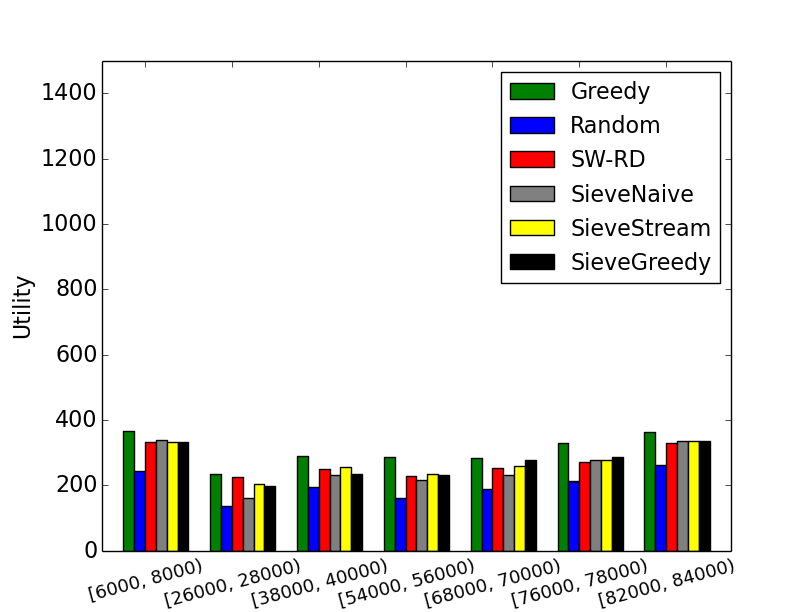
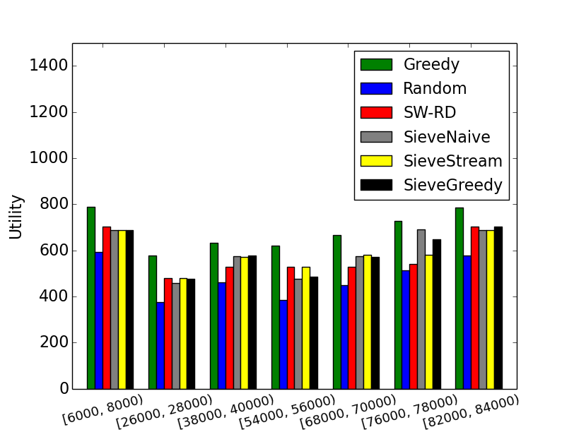
For the application of active set selection, we run experiments on both Eyes and GasSensor datasets. We choose the squared exponential kernel as the kernel function: $\mathcal{K}(x_{i},x_{j})=\exp(-\|x_{i}-x_{j}\|_{2}^{2}/h^{2})$; we set $\sigma=1$ and $h=0.75$. For the application of maximum coverage problem, we run experiments on the WorldCup dataset. For all algorithms, we set $\epsilon=0.2$.

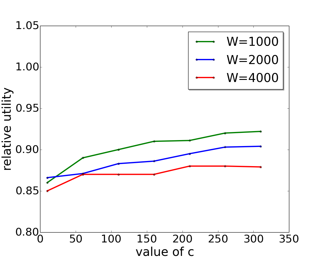
It can be observed from Figure 1, Figure 2 and Figure 3 that the maximum utility given by the standard greedy changes when we slide the window over the data stream. In Figure 1, SieveStream, SW-RD, SieveGreedy and SieveNaive generate results of almost the same quality as the one given by Greedy, and Random gives the worst results in all selected windows. In both Figure 2 and Figure 3, results generated by SW-RD, SieveNaive, SieveGreedy and SieveStream are slightly worse than the one given by Greedy. In most windows, SieveGreedy is as good as SieveStream. SieveNaive also performs well in most windows, but it is worse than Random in some windows. In theory, SW-RD can be worse than SieveStream by a factor of $2$, but our experiments show that solutions returned by the two algorithms have similar utilities. Figure 3c shows in SieveGreedy, increasing $c$ will slightly increase the utility.

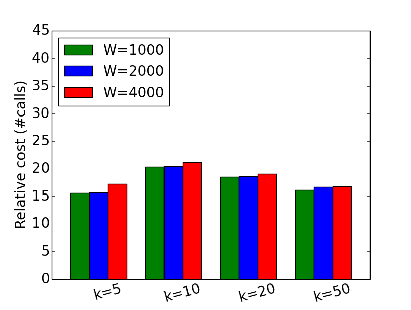
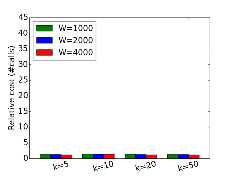
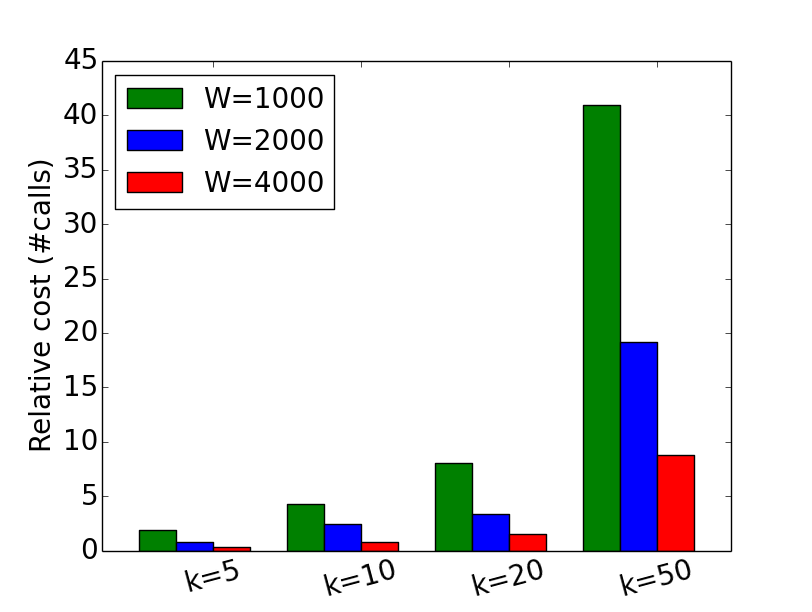
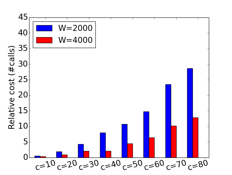
For the comparisons of space/time costs, we only include the results of Eyes dataset due to the space constraints. Similar results can observed on other datasets as well. Figure 4 compares the time costs on Eyes dataset. We measure the time costs by the numbers of function calls (of the submodular function). All results are normalized by the corresponding costs of SieveStream. By Theorem 1 the time cost of SW-RD is independent of $k$ and $W$ once it is normalized by the corresponding cost of SieveStream. This result has been confirmed by Figure 4a. Figure 4b shows that SieveNaive is as fast as SieveStream. Figure 4c shows that increasing $k$ will increase the cost of SieveGreedy, while increasing $W$ will decrease the cost. This is because items in the solution buffers are less likely to expire for small $k$ and large $W$. Figure 4d shows how the time costs of SieveGreedy are affected by the values of $c$.

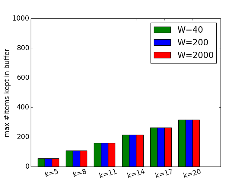
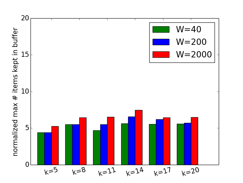
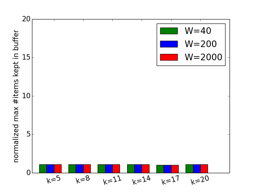
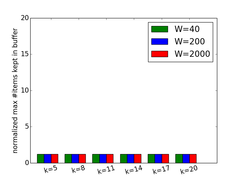
Figure 5 compares the space costs on Eyes dataset. To be consistent with the theorems, we measure the space usages by the maximum numbers of items kept in memory. To compare with the costs of SieveStream, we also normalize the costs of SW-RD, SieveNaive and SieveGreedy by the corresponding costs of SieveStream. Figure 5c and Figure 5d show that the space usages of SieveNaive and SieveGreedy are almost the same as SieveStream.

Summary

We conclude from our experiments that (1) the distribution of data stream changes over sliding windows in our tested datasets; (2) in terms of solution quality, SW-RD, SieveNaive and SieveGreedy generate comparable results as SieveStream, and Random is clearly the worst. SieveNaive can sometimes perform very badly, while SW-RD (the only algorithm with theoretical guarantees) and SieveGreedy are relatively stable; and (3) SieveNaive is the most time and space efficient algorithm among SW-RD, SieveNaive and SieveGreedy, and the performance of SieveGreedy is close for large window size and small $k$. For large window size and small $k$, SieveGreedy runs very fast and the only extra space it uses compared with SieveStream is the buffer of samples (i.e. $B$). Depending on the value of $\epsilon^{-1}\log M$, SW-RD typically uses $10$-$20$x processing time and $10$-$20$x space compared to SieveStream.

References

- [1] M. Arlitt and T. Jin. 1998 world cup web site access logs. http://ita.ee.lbl.gov/html/contrib/WorldCup.html, 1998.
- [2] B. Babcock, M. Datar, and R. Motwani. Sampling from a moving window over streaming data. In SODA, pages 633–634. Society for Industrial and Applied Mathematics, 2002.
- [3] B. Babcock, M. Datar, R. Motwani, and L. O’Callaghan. Maintaining variance and k-medians over data stream windows. In PODS, pages 234–243. ACM, 2003.
- [4] A. Badanidiyuru, B. Mirzasoleiman, A. Karbasi, and A. Krause. Streaming submodular maximization: Massive data summarization on the fly. In SIGKDD, pages 671–680. ACM, 2014.
- [5] J. Bilmes. Lecture notes on submodular optimization. http://j.ee.washington.edu/~bilmes/classes/ee596b_spring_2014/, 2014.
- [6] V. Braverman, H. Lang, K. Levin, and M. Monemizadeh. A unified approach for clustering problems on sliding windows. arXiv preprint arXiv:1504.05553, 2015.
- [7] V. Braverman and R. Ostrovsky. Smooth histograms for sliding windows. In FOCS, pages 283–293, 2007.
- [8] A. Chakrabarti and S. Kale. Submodular maximization meets streaming: matchings, matroids, and more. Math. Program., 154(1-2):225–247, 2015.
- [9] C. Chekuri, S. Gupta, and K. Quanrud. Streaming algorithms for submodular function maximization. In ICALP, pages 318–330, 2015.
- [10] J. Fonollosa, S. Sheik, R. Huerta, and S. Marco. Reservoir computing compensates slow response of chemosensor arrays exposed to fast varying gas concentrations in continuous monitoring. Sensors and Actuators B: Chemical, 215:618–629, 2015.
- [11] J. Gillenwater, A. Kulesza, and B. Taskar. Near-optimal map inference for determinantal point processes. In NIPS, pages 2735–2743, 2012.
- [12] A. Krause and R. G. Gomes. Budgeted nonparametric learning from data streams. In ICML, pages 391–398, 2010.
- [13] R. Kumar, B. Moseley, S. Vassilvitskii, and A. Vattani. Fast greedy algorithms in mapreduce and streaming. ACM Transactions on Parallel Computing, 2(3):14, 2015.
- [14] N. Lawrence, M. Seeger, and R. Herbrich. Fast sparse gaussian process methods: The informative vector machine. In NIPS, number EPFL-CONF-161319, pages 609–616, 2003.
- [15] S. Muthukrishnan. Data streams: Algorithms and applications. Now Publishers Inc, 2005.
- [16] G. L. Nemhauser, L. A. Wolsey, and M. L. Fisher. An analysis of approximations for maximizing submodular set functions—i. Mathematical Programming, 14(1):265–294, 1978.
- [17] O. Roesler. Eeg eye state data set. http://archive.ics.uci.edu/ml/machine-learning-databases/00264/, 2013.
- [18] C. Sanderson. Armadillo: An open source c++ linear algebra library for fast prototyping and computationally intensive experiments. 2010.
- [19] B. Schölkopf and A. J. Smola. Learning with kernels: support vector machines, regularization, optimization, and beyond. MIT press, 2002.
- [20] R. Sipos, A. Swaminathan, P. Shivaswamy, and T. Joachims. Temporal corpus summarization using submodular word coverage. In CIKM, CIKM ’12, pages 754–763, 2012.
- [21] S. Van Vaerenbergh, J. Via, and I. Santamaría. A sliding-window kernel rls algorithm and its application to nonlinear channel identification. In ICASSP, volume 5, pages 789–792. IEEE, 2006.