The Multi-fidelity Multi-armed Bandit

Abstract

We study a variant of the classical stochastic $K$-armed bandit where observing the outcome of each arm is expensive, but cheap approximations to this outcome are available. For example, in online advertising the performance of an ad can be approximated by displaying it for shorter time periods or to narrower audiences. We formalise this task as a multi-fidelity bandit, where, at each time step, the forecaster may choose to play an arm at any one of $M$ fidelities. The highest fidelity (desired outcome) expends cost $\lambda^{(M)}$. The $m$${}^{\textrm{th}}$ fidelity (an approximation) expends $\lambda^{(m)}<\lambda^{(M)}$ and returns a biased estimate of the highest fidelity. We develop MF-UCB, a novel upper confidence bound procedure for this setting and prove that it naturally adapts to the sequence of available approximations and costs thus attaining better regret than naive strategies which ignore the approximations. For instance, in the above online advertising example, MF-UCB would use the lower fidelities to quickly eliminate suboptimal ads and reserve the larger expensive experiments on a small set of promising candidates. We complement this result with a lower bound and show that MF-UCB is nearly optimal under certain conditions.

1 Introduction

Since the seminal work of Robbins [11], the multi-armed bandit has become an attractive framework for studying exploration-exploitation trade-offs inherent to tasks arising in online advertising, finance and other fields. In the most basic form of the $K$-armed bandit [12, 9], we have a set $\mathcal{K}=\{1,\dots,K\}$ of $K$ arms (e.g. $K$ ads in online advertising). At each time step $t=1,2,\dots$, an arm is played and a corresponding reward is realised. The goal is to design a strategy of plays that minimises the regret after $n$ plays. The regret is the comparison, in expectation, of the realised reward against an oracle that always plays the best arm. The well known Upper Confidence Bound (UCB) algorithm [3], achieves regret $\mathcal{O}(K\log(n))$ after $n$ plays (ignoring mean rewards) and is minimax optimal [9].

In this paper, we propose a new take on this important problem. In many practical scenarios of interest, one can associate a cost to playing each arm. Furthermore, in many of these scenarios, one might have access to cheaper approximations to the outcome of the arms. For instance, in online advertising the goal is to maximise the cumulative number of clicks over a given time period. Conventionally, an arm pull maybe thought of as the display of an ad for a specific time, say one hour. However, we may approximate its hourly performance by displaying the ad for shorter periods. This estimate is biased (and possibly noisy), as displaying an ad for longer intervals changes user behaviour. It can nonetheless be useful in gauging the long run click through rate. We can also obtain biased estimates of an ad by displaying it only to certain geographic regions or age groups. Similarly one might consider algorithm selection for machine learning problems [4], where the goal is to be competitive with the best among a set of learning algorithms for a task. Here, one might obtain cheaper approximate estimates of the performance of algorithm by cheaper versions using less data or computation. In this paper, we will refer to such approximations as fidelities. Consider a $2$-fidelity problem where the cost at the low fidelity is $\lambda^{(1)}$ and the cost at the high fidelity is $\lambda^{(2)}$. We will present a cost weighted notion of regret for this setting for a strategy that expends a capital of $\Lambda$ units. A classical $K$-armed bandit strategy such as UCB, which only uses the highest fidelity, can obtain at best $\mathcal{O}(\lambda^{(2)}K\log(\Lambda/\lambda^{(2)}))$ regret [9]. In contrast, this paper will present multi-fidelity strategies that achieve $\mathcal{O}\left((\lambda^{(1)}K+\lambda^{(2)}|\mathcal{K}_{g}|)\log(\Lambda/\lambda^{(2)})\right)$ regret. Here $\mathcal{K}_{g}$ is a (typically) small subset of arms with high expected reward that can be identified using plays at the (cheaper) low fidelity. When $|\mathcal{K}_{g}|<K$ and $\lambda^{(1)}<\lambda^{(2)}$, such a strategy will outperform the more standard UCB algorithms. Intuitively, this is achieved by using the lower fidelities to eliminate several of “bad” arms and reserving expensive higher fidelity plays for a small subset of the most promising arms. We formalise the above intuitions in the sequel. Our main contributions are,

1. A novel formalism for studying bandit tasks when one has access to multiple fidelities for each arm, with each successive fidelity providing a better approximation to the most expensive one.

2. A new algorithm that we call Multi-Fidelity Upper Confidence Bound (MF-UCB) that adapts the classical Upper Confidence Bound (UCB) strategies to our multi-fidelity setting. Empirically, we demonstrate that our algorithm outperforms naive UCB on simulations.

3. A theoretical characterisation of the performance of MF-UCB that shows that the algorithm (a) uses the lower fidelities to explore all arms and eliminates arms with low expected reward, and (b) reserves the higher fidelity plays for arms with rewards close to the optimal value. We derive a lower bound on the regret and demonstrate that MF-UCB is near-optimal on this problem.

Related Work

The $K$-armed bandit has been studied extensively in the past [11, 1, 9]. There has been a flurry of work on upper confidence bound (UCB) methods [2, 3], which adopt the optimism in the face of uncertainty principle for bandits. For readers unfamiliar with UCB methods, we recommend Chapter 2 of Bubeck and Cesa-Bianchi [5]. Our work in this paper builds on UCB ideas, but the multi-fidelity framework poses significantly new algorithmic and theoretical challenges.

There has been some interest in multi-fidelity methods for optimisation in many applied domains of research [7, 10]. However, these works do not formalise or analyse notions of regret in the multi-fidelity setting. Multi-fidelity methods are used in the robotics community for reinforcement learning tasks by modeling each fidelity as a Markov decision process [6]. Zhang and Chaudhuri [16] study active learning with a cheap weak labeler and an expensive strong labeler. The objective of these papers however is not to handle the exploration-exploitation trade-off inherent to the bandit setting. A line of work on budgeted multi-armed bandits [15, 13] study a variant of the $K$-armed bandit where each arm has a random reward and cost and the goal is to play the arm with the highest reward/cost ratio as much as possible. This is different from our setting where each arm has multiple fidelities which serve as an approximation. Recently, in Kandasamy et al. [8] we extended ideas in this work to analyse multi-fidelity bandits with Gaussian process payoffs.

2 The Stochastic $K$-armed Multi-fidelity Bandit

In the classical $K$-armed bandit, each arm $k\in\mathcal{K}=\{1,\dots,K\}$ is associated with a real valued distribution $\theta_{k}$ with mean $\mu_{k}$. Let $\mathcal{K}_{\star}=\mathop{\mathrm{argmax}}_{k\in\mathcal{K}}\mu_{k}$ be the set of optimal arms, $k_{\star}\in\mathcal{K}_{\star}$ be an optimal arm and $\mu_{\star}=\mu_{k_{\star}}$ denote the optimal mean value. A bandit strategy would play an arm $I_{t}\in\mathcal{K}$ at each time step $t$ and observe a sample from $\theta_{I_{t}}$. Its goal is to maximise the sum of expected rewards after $n$ time steps $\sum_{t=1}^{n}\mu_{I_{t}}$, or equivalently minimise the cumulative pseudo-regret $\sum_{t=1}^{n}\mu_{\star}-\mu_{I_{t}}$ for all values of $n$. In other words, the objective is to be competitive, in expectation, against an oracle that plays an optimal arm all the time.

In this work we differ from the usual bandit setting in the following aspect. For each arm $k$, we have access to $M-1$ successively approximate distributions $\theta_{k}^{(1)},\theta_{k}^{(2)},\dots,\theta_{k}^{(M-1)}$ to the desired distribution $\theta_{k}^{(M)}=\theta_{k}$. We will refer to these approximations as fidelities. Clearly, these approximations are meaningful only if they give us some information about $\theta_{k}^{(M)}$. In what follows, we will assume that the $m$${}^{\textrm{th}}$ fidelity mean of an arm is within $\zeta^{(m)}$, a known quantity, of its highest fidelity mean, where $\zeta^{(m)}$, decreasing with $m$, characterise the successive approximations. That is, $|\mu_{k}^{(M)}-\mu_{k}^{(m)}|\leq\zeta^{(m)}$ for all $k\in\mathcal{K}$ and $m=1,\dots,M$, where $\zeta^{(1)}>\zeta^{(2)}>\dots>\zeta^{(M)}=0$ and the $\zeta^{(m)}$’s are known. It is possible for the lower fidelities to be misleading under this assumption: there could exist an arm $k$ with $\mu_{k}^{(M)}<\mu_{\star}=\mu_{k_{\star}}^{(M)}$ but with $\mu_{k}^{(m)}>\mu_{\star}$ and/or $\mu_{k}^{(m)}>\mu_{k_{\star}}^{(m)}$ for any $m<M$. In other words, we wish to explicitly account for the biases introduced by the lower fidelities, and not treat them as just a higher variance observation of an expensive experiment. This problem of course becomes interesting only when lower fidelities are more attractive than higher fidelities in terms of some notion of cost. Towards this end, we will assign a cost $\lambda^{(m)}$ (such as advertising time, money etc.) to playing an arm at fidelity $m$ where $\lambda^{(1)}<\lambda^{(2)}\dots<\lambda^{(M)}$.

Notation: $T^{(m)}_{k,t}$ denotes the number of plays at arm $k$, at fidelity $m$ until $t$ time steps. $T^{(>m)}_{k,t}$ is the number of plays at fidelities greater than $m$. $Q^{(m)}_{t}=\sum_{k\in\mathcal{K}}T^{(m)}_{k,t}$ is the number of fidelity $m$ plays at all arms until time $t$. $\overline{X}^{(m)}_{k,s}$ denotes the mean of $s$ samples drawn from $\theta_{k}^{(m)}$. Denote $\Delta^{(m)}_{k}=\mu_{\star}-\mu_{k}^{(m)}-\zeta^{(m)}$. When $s$ refers to the number of plays of an arm, we will take $1/s=\infty$ if $s=0$. $\overline{A}$ denotes the complement of a set $A\subset\mathcal{K}$. While discussing the intuitions in our proofs and theorems we will use $\asymp,\lesssim,\gtrsim$ to denote equality and inequalities ignoring constants.

Regret in the multi-fidelity setting: A strategy for a multi-fidelity bandit problem, at time $t$, produces an arm-fidelity pair $(I_{t},m_{t})$, where $I_{t}\in\mathcal{K}$ and $m_{t}\in\{1,\dots,M\}$, and observes a sample $X_{t}$ drawn (independently of everything else) from the distribution $\theta_{I_{t}}^{(m_{t})}$. The choice of $(I_{t},m_{t})$ could depend on previous arm-observation-fidelity tuples $\{(I_{i},X_{i},m_{i})\}_{i=1}^{t-1}$. The multi-fidelity setting calls for a new notion of regret. For any strategy $\mathcal{A}$ that expends $\Lambda$ units of the resource, we will define the pseudo-regret $R(\Lambda,\mathcal{A})$ as follows. Let $q_{t}$ denote the instantaneous pseudo-reward at time $t$ and $r_{t}=\mu_{\star}-q_{t}$ denote the instantaneous pseudo-regret. We will discuss choices for $q_{t}$ shortly. Any notion of regret in the multi-fidelity setting needs to account for this instantaneous regret along with the cost of the fidelity at which we played at time $t$, i.e. $\lambda^{(m_{t})}$. Moreover, we should receive no reward (maximum regret) for any unused capital. These observations lead to the following definition,

$$R(\Lambda,\mathcal{A})\;=\;\Lambda\mu_{\star}-\sum_{t=1}^{N}\lambda^{(m_{t})}q_{t}\;=\;\underbrace{\left(\Lambda-\sum_{t=1}^{N}\lambda^{(m_{t})}\right)\mu_{\star}}_{\tilde{r}(\Lambda,\mathcal{A})}\;\;+\;\;\underbrace{\sum_{t=1}^{N}\lambda^{(m_{t})}r_{t}}_{\tilde{R}(\Lambda,\mathcal{A})}.$$ (1)

Above, $N$ is the (random) number of plays within capital $\Lambda$ by $\mathcal{A}$, i.e. the largest $n$ such that $\sum_{t=1}^{n}\lambda^{(m_{t})}\leq\Lambda$. To motivate our choice of $q_{t}$ we consider an online advertising example where $\lambda^{(m)}$ is the advertising time at fidelity $m$ and $\mu_{k}^{(m)}$ is the expected number of clicks per unit time. While we observe from $\theta_{I_{t}}^{(m_{t})}$ at time $t$, we wish to reward the strategy according to its highest fidelity distribution $\theta_{I_{t}}^{(M)}$. Therefore regardless of which fidelity we play we set $q_{t}=\mu_{I_{t}}^{(M)}$. Here, we are competing against an oracle which plays an optimal arm at any fidelity all the time. Note that we might have chosen $q_{t}$ to be $\mu_{I_{t}}^{(m_{t})}$. However, this does not reflect the motivating applications for the multi-fidelity setting that we consider. For instance, a clickbait ad might receive a high number of clicks in the short run, but its long term performance might be poor. Furthermore, for such a choice, we may as well ignore the rich structure inherent to the multi-fidelity setting and simply play the arm $\mathop{\mathrm{argmax}}_{m,k}\mu_{k}^{(m)}$ at each time. There are of course other choices for $q_{t}$ that result in very different notions of regret; we discuss this briefly at the end of Section 7.

The distributions $\theta_{k}^{(m)}$ need to be well behaved for the problem to be tractable. We will assume that they satisfy concentration inequalities of the following form. For all $\epsilon>0$,

$$\forall\,m,\,k,\hskip 21.68121pt\mathbb{P}\big{(}\overline{X}^{(m)}_{k,s}-\mu_{k}^{(m)}>\epsilon\big{)}\;<\;\nu e^{-s\psi(\epsilon)},\hskip 21.68121pt\mathbb{P}\big{(}\overline{X}^{(m)}_{k,s}-\mu_{k}^{(m)}<-\epsilon\big{)}\;<\;\nu e^{-s\psi(\epsilon)}.$$ (2)

Here $\nu>0$ and $\psi$ is an increasing function with $\psi(0)=0$ and is at least increasing linearly $\psi(x)\in\Omega(x)$. For example, if the distributions are sub-Gaussian, then $\psi(x)\in\Theta(x^{2})$.

The performance of a multi-fidelity strategy which switches from low to high fidelities can be worsened by artificially inserting fidelities. Consider a scenario where $\lambda^{(m+1)}$ is only slightly larger than $\lambda^{(m)}$ and $\zeta^{(m+1)}$ is only slightly smaller than $\zeta^{(m)}$. This situation is unfavourable since there isn’t much that can be inferred from the $(m+1)$${}^{\textrm{th}}$ fidelity that cannot already be inferred from the $m$${}^{\textrm{th}}$ by expending the same cost. We impose the following regularity condition to avoid such situations.

Assumption 1.

The $\zeta^{(m)}$’s decay fast enough such that $\sum_{i=1}^{m}\frac{1}{\psi(\zeta^{(i)})}\leq\frac{1}{\psi(\zeta^{(m+1)})}$ for all $m<M$.

Assumption 1 is not necessary to analyse our algorithm, however, the performance of MF-UCB when compared to UCB is most appealing when the above holds. In cases where $M$ is small enough and can be treated as a constant, the assumption is not necessary. For sub-Gaussian distributions, the condition is satisfied for an exponentially decaying $(\zeta^{(1)},\zeta^{(2)},\dots)$ such as $(1/\sqrt{2},1/2,1/2\sqrt{2}\dots)$.

Our goal is to design a strategy $\mathcal{A}_{0}$ that has low expected pseudo-regret $\mathbb{E}[R(\Lambda,\mathcal{A}_{0})]$ for all values of (sufficiently large) $\Lambda$, i.e. the equivalent of an anytime strategy, as opposed to a fixed time horizon strategy, in the usual bandit setting. The expectation is over the observed rewards which also dictates the number of plays $N$. From now on, for simplicity we will write $R(\Lambda)$ when $\mathcal{A}$ is clear from context and refer to it just as regret.

3 The Multi-Fidelity Upper Confidence Bound (MF-UCB) Algorithm

As the name suggests, the MF-UCB algorithm maintains an upper confidence bound corresponding to $\mu_{k}^{(m)}$ for each $m\in\{1,\dots,M\}$ and $k\in\mathcal{K}$ based on its previous plays. Following UCB strategies [3, 2], we define the following set of upper confidence bounds,

$$\mathcal{B}^{(m)}_{k,t}(s)\; =\;\;\overline{X}^{(m)}_{k,s}\,+\,\psi^{-1}\Big{(}\frac{\rho\log t}{s}\Big{)}+\zeta^{(m)},\hskip 14.45377pt\textrm{for all }\;m\in\left\{1,\ldots,M\right\},\;k\in\mathcal{K}$$

$$\mathcal{B}_{k,t}\; =\;\min_{m=1,\dots,M}\mathcal{B}^{(m)}_{k,t}(T^{(m)}_{k,t-1}).$$ (3)

Here $\rho$ is a parameter in our algorithm and $\psi$ is from (2). Each $\mathcal{B}^{(m)}_{k,t}(T^{(m)}_{k,t-1})$ provides a high probability upper bound on $\mu_{k}^{(M)}$ with their minimum $\mathcal{B}_{k,t}$ giving the tightest bound (See Appendix A). Similar to UCB, at time $t$ we play the arm $I_{t}$ with the highest upper bound $I_{t}=\mathop{\mathrm{argmax}}_{k\in\mathcal{K}}\mathcal{B}_{k,t}$.

Since our setup has multiple fidelities associated with each arm, the algorithm needs to determine at each time $t$ which fidelity ($m_{t}$) to play the chosen arm ($I_{t}$). For this consider an arbitrary fidelity $m<M$. The $\zeta^{(m)}$ conditions on $\mu_{k}^{(m)}$ imply a constraint on the value of $\mu_{k}^{(M)}$. If, at fidelity $m$, the uncertainty interval $\psi^{-1}(\rho\log(t)/T^{(m)}_{I_{t},t-1})$ is large, then we have not constrained $\mu_{I_{t}}^{(M)}$ sufficiently well yet. There is more information to be gleaned about $\mu_{I_{t}}^{(M)}$ from playing the arm $I_{t}$ at fidelity $m$. On the other hand, playing at fidelity $m$ indefinitely will not help us much since the $\zeta^{(m)}$ elongation of the confidence band caps off how much we can learn about $\mu_{I_{t}}^{(M)}$ from fidelity $m$; i.e. even if we knew $\mu_{I_{t}}^{(m)}$, we will have only constrained $\mu_{I_{t}}^{(M)}$ to within a $\pm\zeta^{(m)}$ interval. Our algorithm captures this natural intuition. Having selected $I_{t}$, we begin checking at the first fidelity. If $\psi^{-1}(\rho\log(t)/T^{(1)}_{I_{t},t-1})$ is smaller than a threshold $\gamma^{(1)}$ we proceed to check the second fidelity, continuing in a similar fashion. If at any point $\psi^{-1}(\rho\log(t)/T^{(m)}_{I_{t},t-1})\geq\gamma^{(m)}$, we play $I_{t}$ at fidelity $m_{t}=m$. If we go all the way to fidelity $M$, we play at $m_{t}=M$. The resulting procedure is summarised below in Algorithm 1.

• for $t=1,2,\dots$

  1. Choose $I_{t}\in\mathop{\mathrm{argmax}}_{k\in\mathcal{K}}\,\mathcal{B}_{k,t}$.       (See equation (3).)

  2. $m_{t}=\min_{m}\;\{\,m\;|\;\psi^{-1}(\rho\log t/T^{(m)}_{I_{t},t-1})\geq\gamma^{(m)}\;\;\vee\;\;m=M\}$       (See equation (4).)

  3. Play $X\sim\theta_{I_{t}}^{(m_{t})}$.

Algorithm 1  MF-UCB

Choice of $\gamma^{(m)}$: In our algorithm, we choose

$$\gamma^{(m)}=\psi^{-1}\left(\frac{\lambda^{(m)}}{\lambda^{(m+1)}}\psi\big{(}\zeta^{(m)}\big{)}\right)$$ (4)

To motivate this choice, note that if $\Delta^{(m)}_{k}=\mu_{\star}-\mu_{k}^{(m)}-\zeta^{(m)}>0$ then we can conclude that arm $k$ is not optimal. Step 2 of the algorithm attempts to eliminate arms for which $\Delta^{(m)}_{k}\gtrsim\gamma^{(m)}$ from plays above the $m$${}^{\textrm{th}}$ fidelity. If $\gamma^{(m)}$ is too large, then we would not eliminate a sufficient number of arms whereas if it was too small we could end up playing a suboptimal arm $k$ (for which $\mu_{k}^{(m)}>\mu_{\star}$) too many times at fidelity $m$. As will be revealed by our analysis, the given choice represents an optimal tradeoff under the given assumptions.

4 Analysis

We will be primarily concerned with the term $\tilde{R}(\Lambda,\mathcal{A})=\tilde{R}(\Lambda)$ from (1). $\tilde{r}(\Lambda,\mathcal{A})$ is a residual term; it is an artefact of the fact that after the $N+1$${}^{\textrm{th}}$ play, the spent capital would have exceeded $\Lambda$. For any algorithm that operates oblivious to a fixed capital, it can be bounded by $\lambda^{(M)}\mu_{\star}$ which is negligible compared to $\tilde{R}(\Lambda)$. According to the above, we have the following expressions for $\tilde{R}(\Lambda)$:

$$\tilde{R}(\Lambda)\;=\;\sum_{k\in\mathcal{K}}\Delta^{(M)}_{k}\left(\sum_{m=1}^{M}\lambda^{(m)}T^{(m)}_{k,N}\right),$$ (5)

Central to our analysis will be the following partitioning of $\mathcal{K}$. First denote the set of arms whose fidelity $m$ mean is within $\eta$ of $\mu_{\star}$ to be $\mathcal{J}^{(m)}_{\eta}=\{k\in\mathcal{K};\,\mu_{\star}-\mu_{k}^{(m)}\leq\eta\}$. Define $\mathcal{K}^{(1)}\triangleq\overline{\mathcal{J}}^{(1)}_{\zeta^{(1)}+2\gamma^{(1)}}=\{k\in\mathcal{K};\,\Delta^{(1)}_{k}>2\gamma^{(1)}\}$ to be the arms whose first fidelity mean $\mu_{k}^{(1)}$ is at least $\zeta^{(1)}+2\gamma^{(1)}$ below the optimum $\mu_{\star}$. Then we recursively define,

$$\mathcal{K}^{(m)}\triangleq\overline{\mathcal{J}}^{(m)}_{\zeta^{(m)}+2\gamma^{(m)}}\cap\bigg{(}\bigcap_{\ell=1}^{m-1}\mathcal{J}^{(\ell)}_{\zeta^{(\ell)}+2\gamma^{(\ell)}}\bigg{)},\,\forall m\leq M-1,\hskip 13.00806pt\mathcal{K}^{(M)}\triangleq\overline{\mathcal{K}_{\star}}\cap\bigg{(}\bigcap_{\ell=1}^{M-1}\mathcal{J}^{(\ell)}_{\zeta^{(\ell)}+2\gamma^{(\ell)}}\bigg{)}.$$

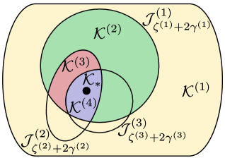
Observe that for all $k\in\mathcal{K}^{(m)}$, $\Delta^{(m)}_{k}>2\gamma^{(m)}$ and $\Delta^{(\ell)}_{k}\leq 2\gamma^{(\ell)}$ for all $\ell<m$. For what follows, for any $k\in\mathcal{K}$, $\llbracket k\rrbracket$ will denote the partition $k$ belongs to, i.e. $\llbracket k\rrbracket=m$ s.t. $k\in\mathcal{K}^{(m)}$. We will see that $\mathcal{K}^{(m)}$ are the arms that will be played at the $m$${}^{\textrm{th}}$ fidelity but can be excluded from fidelities higher than $m$ using information at fidelity $m$. See Fig. 1 for an illustration of these partitions.

Figure 1: Illustration of the partition $\mathcal{K}^{(m)}$’s for a $M=4$ fidelity problem. The sets $\mathcal{J}^{(m)}_{\zeta^{(m)}+2\gamma^{(m)}}$ are indicated next to their boundaries. $\mathcal{K}^{(1)},\mathcal{K}^{(2)},\mathcal{K}^{(3)},\mathcal{K}^{(4)}$ are shown in yellow, green, red and purple respectively. The optimal arms $\mathcal{K}_{\star}$ are shown as a black circle.

4.1 Regret Bound for MF-UCB

Recall that $N=\sum_{m=1}^{M}Q^{(m)}_{N}$ is the total (random) number of plays by a multi-fidelity strategy within capital $\Lambda$. Let $n_{\Lambda}=\lfloor\Lambda/\lambda^{(M)}\rfloor$ be the (non-random) number of plays by any strategy that operates only on the highest fidelity. Since $\lambda^{(m)}<\lambda^{(M)}$ for all $m<M$, $N$ could be large for an arbitrary multi-fidelity method. However, our analysis reveals that for MF-UCB, $N\lesssim n_{\Lambda}$ with high probability. The following theorem bounds $R$ for MF-UCB. The proof is given in Appendix A. For clarity, we ignore the constants but they are fleshed out in the proofs.

Theorem 2 (Regret Bound for MF-UCB).

Let $\rho>4$. There exists $\Lambda_{0}$ depending on $\lambda^{(m)}$’s such that for all $\Lambda>\Lambda_{0}$, MF-UCB satisfies,

$$\frac{\mathbb{E}[R(\Lambda)]}{\log(n_{\Lambda})}\;\lesssim\quad\sum_{k\notin\mathcal{K}_{\star}}\Delta^{(M)}_{k}\cdot\frac{\lambda^{(\llbracket k\rrbracket)}}{\psi(\Delta^{(\llbracket k\rrbracket)}_{k})}\quad\asymp\quad\sum_{m=1}^{M}\sum_{k\in\mathcal{K}^{(m)}}\Delta^{(M)}_{k}\frac{\lambda^{(m)}}{\psi(\Delta^{(m)}_{k})}$$

Let us compare the above bound to UCB whose regret is $\frac{\mathbb{E}[R(\Lambda)]}{\log(n_{\Lambda})}\asymp\sum_{k\notin\mathcal{K}_{\star}}\Delta^{(M)}_{k}\frac{\lambda^{(M)}}{\psi(\Delta^{(M)}_{k})}$. We will first argue that MF-UCB does not do significantly worse than UCB in the worst case. Modulo the $\Delta^{(M)}_{k}\log(n_{\Lambda})$ terms, regret for MF-UCB due to arm $k$ is $R_{k,\textrm{{{MF-UCB}}}}\asymp\lambda^{(\llbracket k\rrbracket)}/\psi(\Delta^{(\llbracket k\rrbracket)}_{k})$. Consider any $k\in\mathcal{K}^{(m)}$, $m<M$ for which $\Delta^{(m)}_{k}>2\gamma^{(m)}$. Since

$$\Delta^{(M)}_{k}\leq\;\Delta^{(\llbracket k\rrbracket)}_{k}+2\zeta^{(\llbracket k\rrbracket)}\;\lesssim\;\psi^{-1}\Big{(}\frac{\lambda^{(\llbracket k\rrbracket+1)}}{\lambda^{(\llbracket k\rrbracket)}}\psi(\Delta^{(\llbracket k\rrbracket)}_{k})\Big{)},$$

a (loose) lower bound for UCB for the same quantity is $R_{k,\textrm{{{UCB}}}}\asymp\lambda^{(M)}/\psi(\Delta^{(M)}_{k})\gtrsim\frac{\lambda^{(M)}}{\lambda^{(\llbracket k\rrbracket+1)}}R_{k,\textrm{{{MF-UCB}}}}$. Therefore for any $k\in\mathcal{K}^{(m)},m<M$, MF-UCB is at most a constant times worse than UCB. However, whenever $\Delta^{(\llbracket k\rrbracket)}_{k}$ is comparable to or larger than $\Delta^{(M)}_{k}$, MF-UCB outperforms UCB by a factor of $\lambda^{(\llbracket k\rrbracket)}/\lambda^{(M)}$ on arm $k$. As can be inferred from the theorem, most of the cost invested by MF-UCB on arm $k$ is at the $\llbracket k\rrbracket$${}^{\textrm{th}}$ fidelity. For example, in Fig. 1, MF-UCB would not play the yellow arms $\mathcal{K}^{(1)}$ beyond the first fidelity (more than a constant number of times). Similarly all green and red arms are played mostly at the second and third fidelities respectively. Only the blue arms are played at the fourth (most expensive) fidelity. On the other hand UCB plays all arms at the fourth fidelity. Since lower fidelities are cheaper MF-UCB achieves better regret than UCB.

It is essential to note here that $\Delta^{(M)}_{k}$ is small for arms in in $\mathcal{K}^{(M)}$. These arms are close to the optimum and require more effort to distinguish than arms that are far away. MF-UCB, like UCB , invests $\log(n_{\Lambda})\lambda^{(M)}/\psi(\Delta^{(M)}_{k})$ capital in those arms. That is, the multi-fidelity setting does not help us significantly with the “hard-to-distinguish” arms. That said, in cases where $K$ is very large and the sets $\mathcal{K}^{(M)}$ is small the bound for MF-UCB can be appreciably better than UCB.

4.2 Lower Bound

Since, $N\geq n_{\Lambda}=\lfloor\Lambda/\lambda^{(M)}\rfloor$, any multi-fidelity strategy which plays a suboptimal arm a polynomial number of times at any fidelity after $n$ time steps, will have worse regret than MF-UCB (and UCB). Therefore, in our lower bound we will only consider strategies which satisfy the following condition.

Assumption 3.

Consider the strategy after $n$ plays at any fidelity. For any arm with $\Delta^{(M)}_{k}>0$, we have $\mathbb{E}[\sum_{m=1}^{M}T^{(m)}_{k,n}]\in o(n^{a})$ for any $a>0$ .

For our lower bound we will consider a set of Bernoulli distributions $\theta_{k}^{(m)}$ for each fidelity $m$ and each arm $k$ with mean $\mu_{k}^{(m)}$. It is known that for Bernoulli distributions $\psi(\epsilon)\in\Theta(\epsilon^{2})$ [14]. To state our lower bound we will further partition the set $\mathcal{K}^{(m)}$ into two sets $\mathcal{K}_{\text{\char 51}}^{(m)},\mathcal{K}_{\text{\char 55}}^{(m)}$ as follows,

$$\mathcal{K}_{\text{\char 51}}^{(m)}=\{k\in\mathcal{K}^{(m)}\;:\Delta^{(\ell)}_{k}\leq 0\;\forall\ell<m\},\hskip 21.68121pt\mathcal{K}_{\text{\char 55}}^{(m)}=\{k\in\mathcal{K}^{(m)}\;:\exists\,\ell<m\,\;\mathrm{s.t.}\;\Delta^{(\ell)}_{k}>0\}.$$

For any $k\in\mathcal{K}^{(m)}$ our lower bound, given below, is different depending on which set $k$ belongs to.

Theorem 4 (Lower bound for $R(\Lambda)$).

Consider any set of Bernoulli reward distributions with $\mu_{\star}\in(1/2,1)$ and $\zeta^{(1)}<1/2$. Then, for any strategy satisfying Assumption 3 the following holds.

$$\liminf_{\Lambda\rightarrow\infty}\frac{\mathbb{E}[R(\Lambda)]}{\log(n_{\Lambda})}\;\geq\;\;\;c\cdot\,\sum_{m=1}^{M}\left[\sum_{k\in\mathcal{K}_{\text{\char 51}}^{(m)}}\Delta^{(M)}_{k}\frac{\lambda^{(m)}}{{\Delta^{(m)}_{k}}^{2}}\;+\;\sum_{k\in\mathcal{K}_{\text{\char 55}}^{(m)}}\Delta^{(M)}_{k}\min_{\ell\in\mathcal{L}_{m}(k)}\frac{\lambda^{(\ell)}}{{\Delta^{(\ell)}_{k}}^{2}}\right]$$ (6)

Here $c$ is a problem dependent constant. $\mathcal{L}_{m}(k)=\{\ell<m:\Delta^{(\ell)}_{k}>0\}\cup\{m\}$ is the union of the $m$${}^{\textrm{th}}$ fidelity and all fidelities smaller than $m$ for which $\Delta^{(\ell)}_{k}>0$.

Comparing this with Theorem 2 we find that MF-UCB meets the lower bound on all arms $k\in\mathcal{K}_{\text{\char 51}}^{(m)},\;\forall m$. However, it may be loose on any $k\in\mathcal{K}_{\text{\char 55}}^{(m)}$. The gap can be explained as follows. For $k\in\mathcal{K}_{\text{\char 55}}^{(m)}$, there exists some $\ell<m$ such that $0<\Delta^{(\ell)}_{k}<2\gamma^{(\ell)}$. As explained previously, the switching criterion of MF-UCB ensures that we do not invest too much effort trying to distinguish whether $\Delta^{(\ell)}_{k}<0$ since $\Delta^{(\ell)}_{k}$ could be very small. That is, we proceed to the next fidelity only if we cannot conclude $\Delta^{(\ell)}_{k}\lesssim\gamma^{(\ell)}$. However, since $\lambda^{(m)}>\lambda^{(\ell)}$ it might be the case that $\lambda^{(\ell)}/{\Delta^{(\ell)}_{k}}^{2}<\lambda^{(m)}/{\Delta^{(m)}_{k}}^{2}$ even though $\Delta^{(m)}_{k}>2\gamma^{(m)}$. Consider for example a two fidelity problem where $\Delta=\Delta^{(1)}_{k}={\Delta^{(2)}_{k}}<2\sqrt{\lambda^{(1)}/\lambda^{(2)}}\zeta^{(1)}$. Here it makes sense to distinguish the arm as being suboptimal at the first fidelity with $\lambda^{(1)}\log(n_{\Lambda})/\Delta^{2}$ capital instead of $\lambda^{(2)}\log(n_{\Lambda})/\Delta^{2}$ at the second fidelity. However, MF-UCB distinguishes this arm at the higher fidelity as $\Delta<2\gamma^{(m)}$ and therefore does not meet the lower bound on this arm. While it might seem tempting to switch based on estimates for $\Delta^{(1)}_{k},{\Delta^{(2)}_{k}}$, this idea is not desirable as estimating ${\Delta^{(2)}_{k}}$ for an arm requires $\log(n_{\Lambda})/\psi({\Delta^{(2)}_{k}})$ samples at the second fidelity; this is is exactly what we are trying to avoid for the majority of the arms via the multi-fidelity setting. We leave it as an open problem to resolve this gap.

5 Proof Sketches

5.1 Theorem 2

First we analyse MF-UCB after $n$ plays (at any fidelity) and control the number of plays of an arm at various fidelities depending on which $\mathcal{K}^{(m)}$ it belongs to. To that end we prove the following.

Lemma 5.

(Bounding $\mathbb{E}[T^{(m)}_{k,n}]$ – Informal) After $n$ time steps of MF-UCB for any $k\in\mathcal{K}$,

$$T^{(\ell)}_{k,n}\lesssim\frac{\log(n)}{\psi(\gamma^{(m)})},\;\;\forall\,\ell<\llbracket k\rrbracket,\hskip 28.90755pt\mathbb{E}[T^{(\llbracket k\rrbracket)}_{k,n}]\lesssim\frac{\log(n)}{\psi(\Delta^{(\llbracket k\rrbracket)}_{k}/2)},\hskip 28.90755pt\mathbb{E}[T^{(>\llbracket k\rrbracket)}_{k,n}]\leq\mathcal{O}(1).$$

The bounds above are illustrated in Table 1. Let $\tilde{R}_{k}(\Lambda)=\sum_{m=1}^{M}\lambda^{(m)}\Delta^{(M)}_{k}T^{(m)}_{k,N}$ be the regret incurred due to arm $k$ and $\tilde{R}_{kn}=\mathbb{E}[\tilde{R}_{k}(\Lambda)|N=n]$. Using Lemma 5 we have,

$$\frac{\tilde{R}_{kn}}{\Delta^{(M)}_{k}\log(n)}\;\lesssim\;\sum_{\ell=1}^{\llbracket k\rrbracket-1}\frac{\lambda^{(\ell)}}{\psi(\gamma^{(m)})}\;\;+\;\;\frac{\lambda^{(\llbracket k\rrbracket)}}{\psi(\Delta^{(\llbracket k\rrbracket)}_{k}/2)}\;+\;o(1)$$ (7)

The next step will be to control the number of plays $N$ within capital $\Lambda$ which will bound $\mathbb{E}[\log(N)]$. While $\Lambda/\lambda^{(1)}$ is an easy bound, we will see that for MF-UCB, $N$ will be on the order of $n_{\Lambda}=\Lambda/\lambda^{(M)}$. For this we will use the following high probability bounds on $T^{(m)}_{k,n}$.

	$\mathcal{K}^{(1)}$	$\mathcal{K}^{(2)}$		$\mathcal{K}^{(m)}$		$\mathcal{K}^{(M)}$	$\mathcal{K}_{\star}$
$\mathbb{E}[T^{(1)}_{k,n}]$	${\color[rgb]{0,0,0}\frac{\log(n)}{\psi(\Delta^{(1)}_{k})}}$	$\frac{\log(n)}{\psi(\gamma^{(1)})}$	…	$\frac{\log(n)}{\psi(\gamma^{(1)})}$	…	$\frac{\log(n)}{\psi(\gamma^{(1)})}$	$\frac{\log(n)}{\psi(\gamma^{(1)})}$
$\mathbb{E}[T^{(2)}_{k,n}]$	$\mathcal{O}(1)$	${\color[rgb]{0,0,0}\frac{\log(n)}{\psi({\Delta^{(2)}_{k}})}}$	…	$\frac{\log(n)}{\psi(\gamma^{(2)})}$	…	$\frac{\log(n)}{\psi(\gamma^{(2)})}$	$\frac{\log(n)}{\psi(\gamma^{(2)})}$
$\vdots$
$\mathbb{E}[T^{(m)}_{k,n}]$		$\mathcal{O}(1)$	…	${\color[rgb]{0,0,0}\frac{\log(n)}{\psi(\Delta^{(m)}_{k})}}$	…	$\frac{\log(n)}{\psi(\gamma^{(m)})}$	$\frac{\log(n)}{\psi(\gamma^{(m)})}$
$\vdots$
$\mathbb{E}[T^{(M)}_{k,n}]$				$\mathcal{O}(1)$		${\color[rgb]{0,0,0}\frac{\log(n)}{\psi(\Delta^{(M)}_{k})}}$	$\Omega(n)$

Table 1: Bounds on the expected number of plays for each $k\in\mathcal{K}^{(m)}$ (columns) at each fidelity (rows) after $n$ time steps (i.e. $n$ plays at any fidelity) in MF-UCB.

Lemma 6.

(Bounding $\mathbb{P}(T^{(m)}_{k,n}>\cdot\;)$ – Informal) After $n$ time steps of MF-UCB for any $k\in\mathcal{K}$,

$$\mathbb{P}\left(T^{(\llbracket k\rrbracket)}_{k,n}\;\gtrsim\;x\cdot\frac{\log(n)}{\psi(\Delta^{(\llbracket k\rrbracket)}_{k}/2)}\right)\;\lesssim\;\frac{1}{n^{x\rho-1}}\,,\hskip 28.90755pt\mathbb{P}\left(T^{(>\llbracket k\rrbracket)}_{k,n}>x\right)\;\lesssim\;\frac{1}{x^{\rho-2}}.$$

We bound the number of plays at fidelities less than $M$ via Lemma 6 and obtain $n/2>\sum_{m=1}^{M-1}Q^{(m)}_{n}$ with probability greater than, say $\delta$, for all $n\geq n_{0}$. By setting $\delta=1/\log(\Lambda/\lambda^{(1)})$, we get $\mathbb{E}[\log(N)]\lesssim\log(n_{\Lambda})$. The actual argument is somewhat delicate since $\delta$ depends on $\Lambda$.

This gives as an expression for the regret due to arm $k$ to be of the form (7) where $n$ is replaced by $n_{\Lambda}$. Then we we argue that the regret incurred by an arm $k$ at fidelities less than $\llbracket k\rrbracket$ (first term in the RHS of (7)) is dominated by $\lambda^{(\llbracket k\rrbracket)}/\psi(\Delta^{(\llbracket k\rrbracket)}_{k})$ (second term). This is possible due to the design of the sets $\mathcal{K}^{(m)}$ and Assumption 1. While Lemmas 5, 6 require only $\rho>2$, we need $\rho>4$ to ensure that $\sum_{m=1}^{M-1}Q^{(m)}_{n}$ remains sublinear when we plug-in the probabilities from Lemma 6. $\rho>2$ is attainable with a more careful design of the sets $\mathcal{K}^{(m)}$. The $\Lambda>\Lambda_{0}$ condition is needed because initially MF-UCB is playing at lower fidelities and for small $\Lambda$, $N$ could be much larger than $n_{\Lambda}$.

5.2 Theorem 4

First we show that for an arm $k$ with $\Delta^{(p)}_{k}>0$ and $\Delta^{(\ell)}_{k}\leq 0$ for all $\ell<p$, any strategy should satisfy

$$R_{k}(\Lambda)\;\gtrsim\;\;\log(n_{\Lambda})\,\Delta^{(M)}_{k}\bigg{[}\min_{\ell\geq p,\Delta^{(\ell)}_{k}>0}\,\frac{\lambda^{(\ell)}}{{\Delta^{(\ell)}_{k}}^{2}}\bigg{]}$$

where $R_{k}$ is the regret incurred due to arm $k$. The proof uses a change of measure argument. The modification has Bernoulli distributions with mean $\tilde{\mu}_{k}^{(\ell)},\ell=1,\dots,M$ where $\tilde{\mu}_{k}^{(\ell)}=\mu_{k}^{(\ell)}$ for all $\ell<m$. Then we push $\tilde{\mu}_{k}^{(\ell)}$ slightly above $\mu_{\star}-\zeta^{(\ell)}$ from $\ell=m$ all the way to $M$ where $\tilde{\mu}_{k}^{(M)}>\mu_{\star}$. To control the probabilities after changing to $\tilde{\mu}_{k}^{(\ell)}$ we use the conditions in Assumption 3. Then for $k\in\mathcal{K}^{(m)}$ we argue that $\lambda^{(\ell)}{\Delta^{(\ell)}_{k}}^{2}\gtrsim\lambda^{(m)}/{\Delta^{(m)}_{k}}^{2}$ using, once again the design of the sets $\mathcal{K}^{(m)}$. This yields the separate results for $k\in\mathcal{K}_{\text{\char 51}}^{(m)},\mathcal{K}_{\text{\char 55}}^{(m)}$.

6 Some Simulations on Synthetic Problems

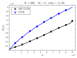
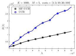
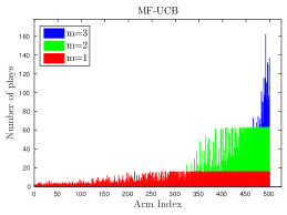
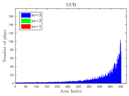
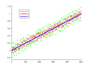
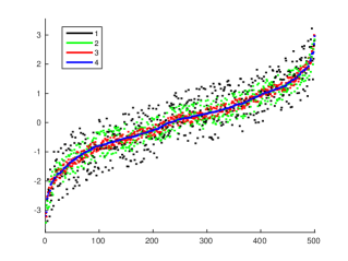
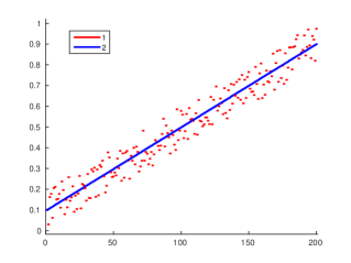
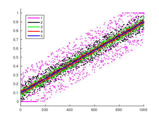
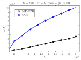
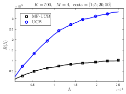
We compare UCB against MF-UCB on a series of synthetic problems. The results are given in Figure 2. Due to space constraints, the details on these experiments are given in Appendix C. Note that MF-UCB outperforms UCB on all these problems. Critically, note that the gradient of the curve is also smaller than that for UCB – corroborating our theoretical insights. We have also illustrated the number of plays by MF-UCB and UCB at each fidelity for one of these problems. The arms are arranged in increasing order of $\mu_{k}^{(M)}$ values. As predicted by our analysis, most of the very suboptimal arms are only played at the lower fidelities. As lower fidelities are cheaper, MF-UCB is able to use more higher fidelity plays at arms close to the optimum than UCB.

Figure 2: Simulations results on the synthetic problems. The first four figures compares UCB against MF-UCB on four synthetic problems. The title states $K,M$ and the costs $\lambda^{(1)},\dots,\lambda^{(M)}$. The first two used Gaussian rewards and the last two used Bernoulli rewards. The last two figures show the number of plays by UCB and MF-UCB on a $K=500,M=3$ problem with Gaussian observations (corresponding to the first figure).

7 Conclusion

We studied a novel framework for studying exploration exploitation trade-offs when cheaper approximations to a desired experiment are available. We propose an algorithm for this setting, MF-UCB, based on upper confidence bound techniques. It uses the cheap lower fidelity plays to eliminate several bad arms and reserves the expensive high fidelity queries for a small set of arms with high expected reward, hence achieving better regret than strategies which ignore multi-fidelity information. We complement this result with a lower bound which demonstrates that MF-UCB is near optimal.

Other settings for bandit problems with multi-fidelity evaluations might warrant different definitions for the regret. For example, consider a gold mining robot where each high fidelity play is a real world experiment of the robot and incurs cost $\lambda^{(2)}$. However, a vastly cheaper computer simulation which incurs $\lambda^{(1)}$ approximate a robot’s real world behaviour. In applications like this $\lambda^{(1)}\ll\lambda^{(2)}$. However, unlike our setting lower fidelity plays may not have any rewards (as simulations do not yield actual gold). Similarly, in clinical trials the regret due to a bad treatment at the high fidelity, would be, say, a dead patient. However, a bad treatment at a lower fidelity may not warrant a large penalty. These settings are quite challenging and we wish to work on them going forward.

Acknowledgements

We would like to thank anonymous reviewers from COLT 2016 and NIPS 2016 for the helpful comments on the content, structure and presentation. This research is partly funded by DOE grant DESC0011114.

Appendix A Upper Bound

We provide the proof in the following three subsections. We will repeatedly use the following result.

Lemma 7.

For all $u>0$, $\sum_{t=u+1}^{\infty}\mathbb{P}(\mathcal{B}_{k_{\star},t}<\mu_{\star})\leq\frac{M\nu}{\rho-2}\frac{1}{u^{\rho-2}}$.

Proof.

The proof is straightforward using a union bound.

$$\mathbb{P}(\mathcal{B}_{k_{\star},t}<\mu_{\star})=\mathbb{P}(\exists m\in\{1,\dots,M\},\;\exists\,1\leq s\leq t-1,\;\;\mathcal{B}^{(m)}_{k_{\star},t}(s)\leq\mu_{\star})$$ (8)

$$\hskip 14.45377pt=\sum_{m=1}^{M}\sum_{s=1}^{t-1}\mathbb{P}\bigg{(}\overline{X}^{(m)}_{k_{\star},s}-\mu_{k_{\star}}^{(m)}<\mu_{\star}-\mu_{k_{\star}}^{(m)}-\zeta^{(m)}-\psi^{-1}\bigg{(}\frac{\rho\log(t)}{s}\bigg{)}\bigg{)}$$

$$\hskip 14.45377pt\leq\;\sum_{m=1}^{M}\sum_{s=1}^{t-1}\nu t^{-\rho}\leq\;M\nu t^{1-\rho}$$

In the third step we have used $\mu_{\star}-\mu_{k}^{(m)}\leq\zeta^{(m)}$. The result follows by bounding the sum with the integral $\sum_{t=u+1}^{\infty}t^{1-\rho}\leq\int_{u}^{\infty}t^{1-\rho}=u^{2-\rho}/(\rho-2)$. ∎

A.1 Proof of Lemma 5

We first provide a formal statement of Lemma 5.

Lemma 8.

Let $m\leq M$ and consider any arm $k\in\mathcal{K}^{(m)}$. After $n$ time steps of $(\gamma,\rho)$-MF-UCB with $\rho>2$ and $\gamma>0$, we have the following bounds on $\mathbb{E}[T^{(\ell)}_{k,n}]\;$ for $\ell=1,\dots,M$.

$$T^{(\ell)}_{k,n}\leq\frac{\rho\log(n)}{\psi(\gamma^{(m)})}+1,\;\;\forall\,\ell<m,\hskip 28.90755pt\mathbb{E}[T^{(m)}_{k,n}]\leq\frac{\rho\log(n)}{\psi(\Delta^{(m)}_{k}/2)}+\kappa_{\rho},\hskip 28.90755pt\mathbb{E}[T^{(>m)}_{k,n}]\leq\kappa_{\rho}.$$

Here, $\kappa_{\rho}=1+\frac{\nu}{2}+\frac{M\nu}{\rho-2}$ is a constant.

Proof.

As $n$ is fixed in this proof, we will write $\mathbb{E}[\cdot],\mathbb{P}(\cdot)$ for $\mathbb{E}[\cdot|N=n],\mathbb{P}(\cdot|N=n)$. Let $\phi^{(m)}_{t}=\lfloor\frac{\rho\log(t)}{\psi(\gamma^{(m)})}\rfloor$. By design of the algorithm we won’t play any arm more than $\phi^{(m)}_{n}+1$ times at any $m<M$. To see this, assume we have already played $\phi^{(m)}_{n}+1$ times at any $t<n$. Then,

$$\psi^{-1}\bigg{(}\frac{\rho\log(t)}{T^{(m)}_{k,t-1}}\bigg{)}<\psi^{-1}\left(\frac{\rho\log(t)}{\rho\log(n)}\psi(\gamma^{(m)})\right)\leq\gamma^{(m)},$$

and we will proceed to the $(m+1)$${}^{\textrm{th}}$ fidelity in step 2 of Algorithm 1. This gives the first part of the theorem. For any $\ell\geq m$ we can avoid the $\frac{1}{\psi(\gamma^{(m)})}$ dependence to obtain tighter bounds.

For the case $\ell=m$, our analysis follows usual multi-armed bandit analyses [5, 2]. For any $u\leq n$, we can bound $T^{(m)}_{k,n}$ via $T^{(m)}_{k,n}\leq u+\sum_{t=u+1}^{n}Z^{(m)}_{k,t,u}$ where $Z^{(m)}_{k,t,u}=\mathbbm{1}{\bf\big{\{}}m_{t}=m\,\wedge\,I_{t}=k\,\wedge\,T^{(m)}_{k,t-1}\geq u{\bf\big{\}}}$. We relax $Z^{(m)}_{k,t,u}$ further via,

$$Z^{(m)}_{k,t,u} \leq\mathbbm{1}{\bf\big{\{}}T^{(\ell)}_{k,t-1}>\phi^{(\ell)}_{t}\;\forall\ell\leq m-1\;\;\;\wedge\;\;\;u\leq T^{(m)}_{k,t-1}\leq\phi^{(m)}_{t}\;\;\;\wedge\;\;\;\mathcal{B}_{k,t}>\mathcal{B}_{k_{\star},t}{\bf\big{\}}}$$

$$\leq\mathbbm{1}{\bf\big{\{}}T^{(m)}_{k,t-1}\geq u\;\;\;\wedge\;\;\;\mathcal{B}^{(m)}_{k,t}(T^{(m)}_{k,t-1})\geq\mu_{\star}{\bf\big{\}}}\;+\;\mathbbm{1}{\bf\big{\{}}\mathcal{B}_{k_{\star},t}<\mu_{\star}{\bf\big{\}}}$$

$$\leq\mathbbm{1}{\bf\big{\{}}\exists\,u\leq s\leq t-1:\;\mathcal{B}^{(m)}_{k,t}(s)>\mu_{\star}{\bf\big{\}}}\;+\;\mathbbm{1}{\bf\big{\{}}\mathcal{B}_{k_{\star},t}<\mu_{\star}{\bf\big{\}}}.$$

This yields, $\mathbb{E}[T^{(m)}_{k,n}]\leq u+\sum_{t=u+1}^{n}\sum_{s=u}^{t-1}\mathbb{P}(\mathcal{B}^{(m)}_{k,t}(s)>\mu_{\star})+\sum_{t=u+1}^{n}\mathbb{P}(\mathcal{B}_{k_{\star},t}<\mu_{\star})$. The third term in this summation is bounded by $M\nu/(\rho-2)$ using Lemma 7. To bound the second, choose $u=\lceil\rho\log(n)/\psi(\Delta^{(m)}_{k}/2)\rceil$. Then,

$$\mathbb{P}(\mathcal{B}^{(m)}_{k,t}(s)>\mu_{\star}) =\mathbb{P}\bigg{(}\overline{X}^{(m)}_{k,s}-\mu_{k}^{(m)}>\mu_{\star}-\mu_{k}^{(m)}-\zeta^{(m)}-\psi^{-1}\Big{(}\frac{\rho\log(t)}{s}\Big{)}\bigg{)}$$

$$\leq\mathbb{P}(\overline{X}^{(m)}_{k,s}-\mu_{k}^{(m)}>\Delta^{(m)}_{k}/2)\leq\nu\exp\bigg{(}-s\psi\Big{(}\frac{\Delta^{(m)}_{k}}{2}\Big{)}\bigg{)}\leq\nu n^{-\rho}$$ (9)

In the second and last steps we have used $\psi^{-1}(\rho\log(t)/s)<\psi^{-1}(\rho\log(t)/u)\leq\Delta^{(m)}_{k}/2$ since $\psi^{-1}$ is increasing and $u>\rho\log(n)/\psi(\Delta^{(m)}_{k}/2)$. Since there are at most $n^{2}$ terms in the summation, the second term is bounded by $\nu n^{2-\rho}/2\leq\nu/2$. Collecting the terms gives the bound on $\mathbb{E}[T^{(m)}_{k,n}]$.

To bound $T^{(>m)}_{k,n}$ we write $T^{(>m)}_{k,n}\leq u+\sum_{t=u+1}^{n}Z^{(>m)}_{k,t,u}$ where

$$Z^{(>m)}_{k,t,u} =\mathbbm{1}{\bf\big{\{}}m_{t}>m\;\;\;\wedge\;\;\;I_{t}=k\;\;\;\wedge\;\;\;T^{(>m)}_{k,t-1}\geq u{\bf\big{\}}}$$

$$\leq\mathbbm{1}{\bf\big{\{}}T^{(\ell)}_{k,t-1}>\phi^{(\ell)}_{t}\,\forall\ell\leq m\;\;\;\wedge\;\;\;\mathcal{B}_{k,t}>\mathcal{B}_{k_{\star},t}\;\;\;\wedge\;\;\;T^{(>m)}_{k,t-1}\geq u{\bf\big{\}}}$$

$$\leq\mathbbm{1}{\bf\big{\{}}T^{(m)}_{k,t-1}>\phi^{(m)}_{t}\;\;\;\wedge\;\;\;\mathcal{B}^{(m)}_{k,t}(T^{(m)}_{k,t-1})>\mu_{\star}{\bf\big{\}}}+\mathbbm{1}{\bf\big{\{}}\mathcal{B}_{k_{\star},t}<\mu_{\star}{\bf\big{\}}}$$

$$\leq\mathbbm{1}{\bf\big{\{}}\exists\,\phi^{(m)}_{t}+1\leq s\leq t-1:\;\mathcal{B}^{(m)}_{k,t}(s)>\mu_{\star}{\bf\big{\}}}+\mathbbm{1}{\bf\big{\{}}\mathcal{B}_{k_{\star},t}<\mu_{\star}{\bf\big{\}}}$$

This yields, $\mathbb{E}[T^{(>m)}_{k,n}]\leq u+\sum_{t=u+1}^{n}\sum_{s=\phi^{(m)}_{t}+1}^{t-1}\mathbb{P}(\mathcal{B}^{(m)}_{k,t}(s)>\mu_{\star})\;+\;\sum_{t=u+1}^{n}\mathbb{P}(\mathcal{B}_{k_{\star},t}<\mu_{\star})$. The inner term inside the double summation can be bounded via,

$$\mathbb{P}(\mathcal{B}^{(m)}_{k,t}(s)>\mu_{\star}) =\mathbb{P}\left(\overline{X}^{(m)}_{k,s}-\mu_{k}^{(m)}>\mu_{\star}-\mu_{k}^{(m)}-\zeta^{(m)}-\psi^{-1}\Big{(}\frac{\rho\log(t)}{s}\Big{)}\right)$$

$$\leq\mathbb{P}(\overline{X}^{(m)}_{k,s}-\mu_{k}^{(m)}>\Delta^{(m)}_{k}-\gamma^{(m)})\leq\nu\exp(-s\psi(\Delta^{(m)}_{k}-\gamma^{(m)}))$$

$$\leq\nu\exp\left(-\frac{\psi(\Delta^{(m)}_{k}-\gamma^{(m)})}{\psi(\gamma^{(m)})}\rho\log(t)\right)\leq\nu t^{-\rho}$$ (10)

The second step follows from $s>\phi^{(m)}_{t}>\rho\log(t)/\psi(\gamma^{(m)})$ and the last step uses $\psi(\Delta^{(m)}_{k}-\gamma^{(m)})>\psi(\gamma^{(m)})$ when $\Delta^{(m)}_{k}>2\gamma^{(m)}$. To bound the summation, we use $u=1$ and bound it by an integral: $\sum_{t=u+1}^{n}t^{-\rho+1}\leq 1/(2u^{\rho-2})\leq 1/2$. Collecting the terms gives the bound on $\mathbb{E}[T^{(>m)}_{k,n}]$. ∎

A.2 Proof of Lemma 6

We first provide a formal statement of Lemma 6.

Lemma 9.

Consider any arm $k\in\mathcal{K}^{(m)}$. For $(\gamma,\rho)$-MF-UCB with $\rho>2$ and $\gamma>0$, we have the following concentration results for $\ell=1,\dots,M$ for any $x\geq 1$.

$$\mathbb{P}\left(T^{(m)}_{k,n}>x\bigg{(}1+\frac{\rho\log(n)}{\psi(\Delta^{(m)}_{k}/2)}\bigg{)}\right)\; \leq\;\frac{\nu\tilde{\kappa}^{(m)}_{k,\rho}}{(x\cdot\log(n))^{\rho-1}}+\frac{\nu}{n^{x\rho-1}}.$$

$$\mathbb{P}\left(T^{(>m)}_{k,n}>x\right)\; \leq\;\frac{M\nu}{\rho-1}\frac{1}{x^{\rho-1}}+\frac{1}{(\rho-2)x^{\rho-2}}$$

Here, $\tilde{\kappa}^{(m)}_{k,\rho}=\frac{M}{\rho-1}\left(\frac{\psi(\Delta^{(m)}_{k}/2)}{\rho}\right)^{\rho-1}$.

Proof.

For the first inequality, we modify the analysis in Audibert et al. [2] to the multi-fidelity setting. We begin with the following observation for all $u\in\mathbb{N}$.

$$\{\forall\,t:\,u+1\leq t\leq n,\mathcal{B}^{(m)}_{k,t}(u)\leq\mu_{\star}\}\;\cap$$ (11)

$$\hskip 14.45377pt\bigcap_{m=1}^{M}\{\forall\,1\leq s\leq n-u:\mathcal{B}^{(m)}_{k_{\star},u+s}(s)>\mu_{\star}\}\;\;\implies\;\;T^{(m)}_{k,n}\leq u$$

To prove this, consider $s^{(m)},m=1,\dots,M$ such that $s^{(1)}\geq 1$, $s^{(m)}\geq 0,\forall m\neq 1$. For all $u+\sum_{m=1}^{M}s^{(m)}\leq t\leq n$ and for all $\ell=1,\dots,M$ we have

$$\mathcal{B}^{(\ell)}_{k_{\star},t}(s^{(\ell)})\geq\mathcal{B}^{(\ell)}_{k_{\star},u+s}(s^{(\ell)})\;>\;\mu_{\star}\geq\mathcal{B}^{(m)}_{k,t}(u)\geq\mathcal{B}^{(m)}_{k,t}(T^{(m)}_{k,t-1}).$$

This means that arm $k$ will not be the $\mathcal{B}_{k,t}$ maximiser at any time $u<t<n$ and consequently it won’t be played more than $u+1$ times at the $m$${}^{\textrm{th}}$ fidelity. Via the union bound we have,

$$\mathbb{P}(T^{(m)}_{k,n}>u) \leq\sum_{t=u+1}^{n}\mathbb{P}(\mathcal{B}^{(m)}_{k,t}(u)>\mu_{\star})+\sum_{m=1}^{M}\sum_{s=1}^{n-u}\mathbb{P}(\mathcal{B}^{(m)}_{k_{\star},u+s}(s)<\mu_{\star}).$$

We will use $u=\lceil x(1+\rho\log(n)/\psi(\Delta^{(m)}_{k}/2))\rceil$. Bounding the inner term of the second double summation closely mimics the calculations in (8) via which it can be shown $\mathbb{P}(\mathcal{B}^{(m)}_{k_{\star},u+s}(s)<\mu_{\star})\leq\nu(u+s)^{-\rho}$. The second term is then bounded by an integral as follows,

$$\sum_{m=1}^{M}\sum_{s=1}^{n-u}\mathbb{P}(\mathcal{B}^{(m)}_{k_{\star},u+s}(s)<\mu_{\star})\leq M\sum_{s=1}^{n-u}\nu(u+s)^{-\rho}\leq M\nu\int_{u}^{n}t^{-\rho}\leq\frac{M\nu u^{1-\rho}}{\rho-1}\leq\frac{\nu\tilde{\kappa}^{(m)}_{k,\rho}}{(x\cdot\log(n))^{\rho-1}}$$

The inner term of the first summation mimics the calculations in (9). Noting that $s>x\rho\log(n)/\psi(\Delta^{(m)}_{k}/2)$ it can be shown $\mathbb{P}(\mathcal{B}^{(m)}_{k,t}(u)>\mu_{\star})\leq\nu n^{-\rho x}$ which bounds the outer summation by $\nu n^{-\rho x+1}$. This proves the first concentration result.

For the second, we begin with the following observation for all $u\in\mathbb{N}$.

$$\{\forall\,t:\,u+1\leq t\leq n,\;\;\mathcal{B}^{(m)}_{k,t}(T^{(m)}_{k,t-1})\leq\mu_{\star}\;\;\;\vee\;\;\;T^{(m)}_{k,t-1}\leq\phi^{(m)}_{t}\}\;\cap$$ (12)

$$\hskip 86.72377pt\bigcap_{m=1}^{M}\{\forall\,1\leq s\leq n-u:\mathcal{B}^{(m)}_{k_{\star},u+s}(s)>\mu_{\star}\}\;\;\implies\;\;T^{(>m)}_{k,n}\leq u$$

To prove this first note that when $T^{(m)}_{k,t-1}\leq\phi^{(m)}_{t}$ we will play at the $m$${}^{\textrm{th}}$ fidelity or lower. Otherwise, consider $s^{(m)},m=1,\dots,M$ such that $s^{(1)}\geq 1$ and $s^{(m)}\geq 0,\forall m$. For all $u+\sum_{m=1}^{M}s^{(m)}\leq t\leq n$ and for all $\ell=1,\dots,M$ we have

$$\mathcal{B}^{(\ell)}_{k_{\star},t}(s^{(\ell)})\geq\mathcal{B}^{(\ell)}_{k_{\star},u+s}(s^{(\ell)})\;>\;\mu_{\star}\geq\mathcal{B}^{(m)}_{k,t}(T^{(m)}_{k,t-1}).$$

This means that arm $k$ will not be played at time $t$ and consequently for any $t>u$. After a further relaxation we get,

$$\mathbb{P}(T^{(>m)}_{k,n}>u) \leq\sum_{t=u+1}^{n}\sum_{s=\phi^{(m)}_{t}+1}^{t-1}\mathbb{P}(\mathcal{B}^{(m)}_{k,t}(s)>\mu_{\star})+\sum_{m=1}^{M}\sum_{s=1}^{n-u}\mathbb{P}(\mathcal{B}^{(m)}_{k_{\star},u+s}(s)<\mu_{\star})$$

The second summation is bounded via $\frac{M\nu}{(\rho-1)u^{\rho-1}}$. Following an analysis similar to (10), the inner term of the first summation can be bounded by $\nu t^{-\rho}$ which bounds the first term by $u^{2-\rho}/(\rho-2)$. The result follows by using $u=x$ in (12). ∎

A.3 Proof of Theorem 2

We first establish the following Lemma.

Lemma 10 (Regret of MF-UCB).

Let $\rho>4$. There exists $\Lambda_{0}$ depending on $\lambda^{(1)},\lambda^{(M)}$ such that for all $\Lambda>\Lambda_{0}$, $(\gamma,\rho)$-MF-UCB satisfies,

$$\mathbb{E}[R(\Lambda)]\leq\mu_{\star}\lambda^{(M)}\,+\,\sum_{k=1}^{K}\Delta^{(M)}_{k}\left(\sum_{\ell=1}^{[k]-1}\lambda^{(\ell)}\frac{\rho(\log(n_{\Lambda})+c)}{\psi(\gamma^{(\ell)})}\,+\,\lambda^{(\llbracket k\rrbracket)}\frac{\rho(\log(n_{\Lambda})+c)}{\psi(\Delta^{(\llbracket k\rrbracket)}_{k}/2)}\,+\mu_{\star}\kappa_{\rho}\lambda^{(M)}\right)$$

Here $c=1+\log(2)$ and $\kappa_{\rho}=1+\frac{\nu}{\rho-2}+\frac{M\nu}{\rho-2}$ are constants.

Denote the set of arms “above" $\mathcal{K}^{(m)}$ by $\widehat{\mathcal{K}}^{(m)}=\bigcup_{\ell=m+1}^{M}\mathcal{K}^{(\ell)}$ and those “below" $\mathcal{K}^{(m)}$ by ${\mathchoice{{\ooalign{\hbox{\raise 7.09259pt\hbox{\scalebox{1.0}[-1.0]{\lower 7.09259pt\hbox{$\displaystyle\widehat{\vrule width=0.0pt,height=6.83331pt\vrule height=0.0pt,width=7.7778pt}$}}}}\cr\hbox{$\displaystyle\mathcal{K}$}}}}{{\ooalign{\hbox{\raise 7.09259pt\hbox{\scalebox{1.0}[-1.0]{\lower 7.09259pt\hbox{$\textstyle\widehat{\vrule width=0.0pt,height=6.83331pt\vrule height=0.0pt,width=7.7778pt}$}}}}\cr\hbox{$\textstyle\mathcal{K}$}}}}{{\ooalign{\hbox{\raise 6.40926pt\hbox{\scalebox{1.0}[-1.0]{\lower 6.40926pt\hbox{$\scriptstyle\widehat{\vrule width=0.0pt,height=4.78333pt\vrule height=0.0pt,width=5.44446pt}$}}}}\cr\hbox{$\scriptstyle\mathcal{K}$}}}}{{\ooalign{\hbox{\raise 5.9537pt\hbox{\scalebox{1.0}[-1.0]{\lower 5.9537pt\hbox{$\scriptscriptstyle\widehat{\vrule width=0.0pt,height=3.41666pt\vrule height=0.0pt,width=3.8889pt}$}}}}\cr\hbox{$\scriptscriptstyle\mathcal{K}$}}}}}\vphantom{\mathcal{K}}^{(m)}=\bigcup_{\ell=1}^{m-1}\mathcal{K}^{(\ell)}$. We first observe,

$$\bigg{(}\forall\,m\leq M-1,\;\forall k\in\mathcal{K}^{(m)},\;\;T^{(m)}_{k,n}\leq x\bigg{(}1+\frac{\rho\log(n)}{\psi(\Delta^{(m)}_{k}/2)}\bigg{)}\;\;\;\wedge\;\;\;T^{(>m)}_{k,n}\leq y\bigg{)}$$ (13)

$$\implies\sum_{m=1}^{M-1}Q^{(m)}_{n}\;\leq\;Ky\;+\;\sum_{m=1}^{M-1}\sum_{k\in\mathcal{K}^{(m)}}x\bigg{(}1+\frac{\rho\log(n)}{\psi(\Delta^{(m)}_{k}/2)}\bigg{)}+\sum_{m=1}^{M-1}|\widehat{\mathcal{K}}^{(m)}|\left(1+\frac{\rho\log(n)}{\psi(\gamma^{(m)})}\right)$$

To prove this we first note that the LHS of (13) is reducible to,

$$\forall\,m\leq M-1,\;\;Q^{(m)}_{n}\leq\sum_{k\in{\mathchoice{{\ooalign{\hbox{\raise 6.40926pt\hbox{\scalebox{1.0}[-1.0]{\lower 6.40926pt\hbox{$\displaystyle\widehat{\vrule width=0.0pt,height=4.78333pt\vrule height=0.0pt,width=5.44446pt}$}}}}\cr\hbox{$\displaystyle\mathcal{K}$}}}}{{\ooalign{\hbox{\raise 6.40926pt\hbox{\scalebox{1.0}[-1.0]{\lower 6.40926pt\hbox{$\textstyle\widehat{\vrule width=0.0pt,height=4.78333pt\vrule height=0.0pt,width=5.44446pt}$}}}}\cr\hbox{$\textstyle\mathcal{K}$}}}}{{\ooalign{\hbox{\raise 5.93092pt\hbox{\scalebox{1.0}[-1.0]{\lower 5.93092pt\hbox{$\scriptstyle\widehat{\vrule width=0.0pt,height=3.34833pt\vrule height=0.0pt,width=3.81111pt}$}}}}\cr\hbox{$\scriptstyle\mathcal{K}$}}}}{{\ooalign{\hbox{\raise 5.61203pt\hbox{\scalebox{1.0}[-1.0]{\lower 5.61203pt\hbox{$\scriptscriptstyle\widehat{\vrule width=0.0pt,height=2.39166pt\vrule height=0.0pt,width=2.72223pt}$}}}}\cr\hbox{$\scriptscriptstyle\mathcal{K}$}}}}}\vphantom{\mathcal{K}}^{(m)}}T^{(m)}_{k,n}\;+\;\sum_{k\in\mathcal{K}^{(m)}}x\bigg{(}1+\frac{\rho\log(n)}{\psi(\Delta^{(m)}_{k}/2)}\bigg{)}+\sum_{k\in\widehat{\mathcal{K}}^{(m)}}\left(1+\frac{\rho\log(n)}{\psi(\gamma^{(m)})}\right)$$

The statement follows by summing the above from $m=1,\dots,M-1$ and rearranging the $T^{(>m)}_{k,n}$ terms to obtain,

$$\sum_{m=1}^{M-1}\sum_{k\in{\mathchoice{{\ooalign{\hbox{\raise 6.40926pt\hbox{\scalebox{1.0}[-1.0]{\lower 6.40926pt\hbox{$\displaystyle\widehat{\vrule width=0.0pt,height=4.78333pt\vrule height=0.0pt,width=5.44446pt}$}}}}\cr\hbox{$\displaystyle\mathcal{K}$}}}}{{\ooalign{\hbox{\raise 6.40926pt\hbox{\scalebox{1.0}[-1.0]{\lower 6.40926pt\hbox{$\textstyle\widehat{\vrule width=0.0pt,height=4.78333pt\vrule height=0.0pt,width=5.44446pt}$}}}}\cr\hbox{$\textstyle\mathcal{K}$}}}}{{\ooalign{\hbox{\raise 5.93092pt\hbox{\scalebox{1.0}[-1.0]{\lower 5.93092pt\hbox{$\scriptstyle\widehat{\vrule width=0.0pt,height=3.34833pt\vrule height=0.0pt,width=3.81111pt}$}}}}\cr\hbox{$\scriptstyle\mathcal{K}$}}}}{{\ooalign{\hbox{\raise 5.61203pt\hbox{\scalebox{1.0}[-1.0]{\lower 5.61203pt\hbox{$\scriptscriptstyle\widehat{\vrule width=0.0pt,height=2.39166pt\vrule height=0.0pt,width=2.72223pt}$}}}}\cr\hbox{$\scriptscriptstyle\mathcal{K}$}}}}}\vphantom{\mathcal{K}}^{(m)}}T^{(m)}_{k,n}=\sum_{m=1}^{M-1}\sum_{\ell=1}^{m-1}\sum_{k\in\mathcal{K}^{(\ell)}}T^{(m)}_{k,n}=\sum_{m=1}^{M-2}\sum_{k\in\mathcal{K}^{(m)}}\sum_{\ell=m+1}^{M-1}T^{(\ell)}_{k,n}\leq\;\sum_{m=1}^{M-2}\sum_{k\in\mathcal{K}^{(m)}}T^{(>m)}_{k,n}$$

$$\hskip 14.45377pt\;\leq\;(K-|\mathcal{K}^{(M-1)}\cup\mathcal{K}^{(M)}\cup\mathcal{K}_{\star}|)y\;\leq\;Ky.$$

Now for the given $\Lambda$ under consideration, define $\delta_{\Lambda}=\frac{1}{\log(\Lambda/\lambda^{(1)})}$. In addition define,

$$x_{n,\delta} =\max\left(\;\;1\;\;,\;\;\frac{1}{\rho}\left(3+\frac{\log(2\nu\pi^{2}K/(3\delta))}{\log(n)}\right)\;\;,\;\;\left(\frac{2\pi^{2}K\nu M}{3(\rho-1)\delta}\right)^{\frac{1}{\rho-1}}\frac{\psi(\Delta^{(m)}_{k}/2)}{\rho}n^{\frac{2}{\rho-1}}\right).$$

$$y_{n,\delta} =\max\left(\;\;1\;\;,\;\;\left(\frac{2\pi^{2}KM\nu}{3(\rho-1)\delta}\right)^{\frac{1}{\rho-1}}n^{\frac{2}{\rho-1}}\;\;,\;\;\left(\frac{\pi^{2}K}{3\delta}\right)^{\frac{1}{\rho-2}}n^{\frac{2}{\rho-2}}\right).$$

Now choose $n_{0,\Lambda}$ to be the smallest $n$ such that the following holds for all $n\geq n_{0,\Lambda}$.

$$\frac{n}{2}\;\geq\;Ky_{n,{\delta_{\Lambda}}}\;+\;\sum_{m=1}^{M-1}\sum_{k\in\mathcal{K}^{(m)}}x_{n,{\delta_{\Lambda}}}\bigg{(}1+\frac{\rho\log(n)}{\psi(\Delta^{(m)}_{k}/2)}\bigg{)}+\sum_{m=1}^{M-1}\sum_{k\in\widehat{\mathcal{K}}^{(m)}}1+\frac{\rho\log(n)}{\psi(\gamma)},$$ (14)

For such an $n_{0,\Lambda}$ to exist, for a given $\Lambda$, we need both $x_{n},y_{n}$ sublinear. This is true since $\rho>4$. In addition, observe that $n_{0,\Lambda}$ grows only polylogarithmically in $\Lambda$ since (14) reduces to $n^{p}\gtrsim(\log(\Lambda))^{1/2}$ where $p>0$ depends on our choice of $\rho$.

By (13), the RHS of (14) is an upper bound on the number of plays at fidelities lower than $M$. Therefore, for all $n\geq n_{0,\Lambda}$,

$$\mathbb{P}\Big{(}Q^{(M)}_{n}<\frac{n}{2}\Big{)} \leq\sum_{m=1}^{M-1}\sum_{k\in\mathcal{K}^{(m)}}\mathbb{P}\bigg{(}T^{(m)}_{k,n}>x_{n,\delta}\bigg{(}1+\frac{\rho\log(n)}{\psi(\Delta^{(m)}_{k}/2)}\bigg{)}\bigg{)}+\mathbb{P}\bigg{(}T^{(>m)}_{k,n}>y_{n,\delta}\bigg{)}$$ (15)

$$\leq\sum_{m=1}^{M-1}\sum_{k\in\mathcal{K}^{(m)}}\frac{\nu}{n^{\rho x_{n,{\delta_{\Lambda}}}-1}}+\frac{\nu\tilde{\kappa}^{(m)}_{k,\rho}}{(x_{n,{\delta_{\Lambda}}}\log(n))^{\rho-1}}+\frac{\nu M}{(\rho-1)y_{n,{\delta_{\Lambda}}}^{\rho-1}}+\frac{1}{2y_{n,{\delta_{\Lambda}}}^{\rho-2}}$$

$$\leq K\left(4\times\frac{3\delta}{2Kn^{2}\pi^{2}}\right)\leq\frac{6\delta}{n^{2}\pi^{2}}.$$

The last step follows from the fact that each of the four terms inside the summation in the second line are $\leq 3\delta/(2Kn^{2}\pi^{2})$. For the last term we have used that $(\rho-2)/2>1$ and that $3\delta/(\pi^{2}K)$ is smaller than $1$. Note that the double summation just enumerates over all arms in $\mathcal{K}$.

We can now specify the conditions on $\Lambda_{0}$. $\Lambda_{0}$ should be large enough so that for all $\Lambda\geq\Lambda_{0}$, we have $\lfloor\Lambda/\lambda^{(M)}\rfloor\geq n_{0,\Lambda}$. Such an $\Lambda_{0}$ exists since $n_{0,\Lambda}$ grows only polylogarithmically in $\Lambda$. This ensures that we have played a sufficient numer of rounds to apply the concentration result in (15).

Let the (random) expended capital after $n$ rounds of MF-UCB be $\Omega(n)$. Let $\mathcal{E}=\{\exists n\geq n_{0,\Lambda}:\Omega(n)<n\lambda^{(M)}/2\}$. Since $\Omega(n)\geq\lambda^{(M)}Q^{(M)}_{n}$, by using the union bound on (15) we have $\mathbb{P}(\mathcal{E})\leq\delta_{\Lambda}$. Therefore,

$$\mathbb{P}\bigg{(}N>\frac{2\Lambda}{\lambda^{(M)}}\bigg{)}\;=\;\mathbb{P}\left(N>\frac{2\Lambda}{\lambda^{(M)}}\Big{|}\mathcal{E}\right)\underbrace{\mathbb{P}(\mathcal{E})}_{\leq\,\delta_{\Lambda}}\;+\;\underbrace{\mathbb{P}\left(N>\frac{2\Lambda}{\lambda^{(M)}}\Big{|}\mathcal{E}^{c}\right)}_{=\,0}\mathbb{P}(\mathcal{E}^{c})\;<\;\delta_{\Lambda}$$

The last step uses the following reasoning: Conditioned on $\mathcal{E}^{c}$, $n>2\Omega(n)/\lambda^{(M)}$ is false for $n>n_{0,\Lambda}$. In particular, it is true for the random number of plays $N$ since $\Lambda>\Lambda_{0}\implies N\geq n_{0,\Lambda}$. Now, clearly $\Lambda>\Omega(N)$ and therefore $N>2\Lambda/\lambda^{(M)}$ is also false.

By noting that $n_{\Lambda}=\Lambda/\lambda^{(M)}$ and that $\log(\Lambda/\lambda^{(1)})$ is always an upper bound on $\log(N)$, we have,

$$\mathbb{E}[\log(N)]\leq\log(2n_{\Lambda})\mathbb{P}(N<2n_{\Lambda})+\log\left(\frac{\Lambda}{\lambda^{(1)}}\right)\mathbb{P}(N>2n_{\Lambda})\;\leq\;\log(n_{\Lambda})+1+\log(2)$$ (16)

Lemma 10 now follows by an application of Lemma 5. First we condition on $N=n$ to obtain,

$$\mathbb{E}[R(\Lambda)|N=n]\;\leq\;\mu_{\star}\lambda^{(M)}\;\;+\;\;\sum_{k=1}^{K}\sum_{m=1}^{M}\Delta^{(M)}_{k}\lambda^{(m)}T^{(m)}_{k,n}$$

$$\hskip 14.45377pt\leq\;\mu_{\star}\lambda^{(M)}\,+\;\sum_{k=1}^{K}\Delta^{(M)}_{k}\left(\sum_{\ell=1}^{[k]-1}\lambda^{(\ell)}\frac{\rho\log(n)}{\psi(\gamma^{(m)})}\;\;+\;\lambda^{(\llbracket k\rrbracket)}\frac{\rho\log(n)}{\psi(\Delta^{(\llbracket k\rrbracket)}_{k}/2)}\;+\kappa_{\rho}\lambda^{(M)}\right)$$

The theorem follows by plugging in the above in $\mathbb{E}[R(\Lambda)]=\mathbb{E}[\mathbb{E}[R(\Lambda)|N]]$ and using the bound for $\mathbb{E}[\log(N)]$ in (16).

We can now bound the regret for MF-UCB.

Proof of Theorem 2.

Recall that $\psi(\gamma^{(m)})=\frac{\lambda^{(m)}}{\lambda^{(m+1)}}\psi(\zeta^{(m)})$. Plugging this into Lemma 10 we get

$$\mathbb{E}[R(\Lambda)] \leq\;\mu_{\star}\lambda^{(M)}\;+\;\sum_{k=1}^{K}\Delta^{(M)}_{k}\left(\sum_{\ell=1}^{[k]-1}\lambda^{(\ell+1)}\frac{\rho(\log(n_{\Lambda})+c)}{\psi(\zeta^{(\ell)})}\;\;+\;\lambda^{(\llbracket k\rrbracket)}\frac{\rho(\log(n_{\Lambda})+c)}{\psi(\Delta^{(\llbracket k\rrbracket)}_{k}/2)}\;+\kappa_{\rho}\lambda^{(M)}\right)$$

$$\leq\;\mu_{\star}\lambda^{(M)}\;+\;\sum_{k=1}^{K}\Delta^{(M)}_{k}\cdot\lambda^{(\llbracket k\rrbracket)}\rho(\log(n_{\Lambda})+c)\left(\frac{2}{\psi(\zeta^{(\llbracket k\rrbracket-1)})}+\frac{1}{\psi(\Delta^{(\llbracket k\rrbracket)}_{k}/2)}\right)+\Delta^{(M)}_{k}\kappa_{\rho}\lambda^{(M)}$$

The second step uses Assumption 1. The theorem follows by noting that for any $k\in\mathcal{K}^{(m)}$ and $\ell<m$, $\Delta^{(m)}_{k}=\Delta^{(\ell)}_{k}+\zeta^{(\ell)}-\zeta^{(m)}+\mu_{k}^{(\ell)}-\mu_{k}^{(M)}+\mu_{k}^{(M)}-\mu_{k}^{(m)}\leq 2\gamma^{(\ell)}+2\zeta^{(\ell)}\leq 4\zeta^{(\ell)}$. Therefore $1/\psi(\Delta^{(m)}_{k})>c_{1}/\psi(\zeta^{(\ell)})$ where $c_{1}$ depends on $\psi$ (for sub-Gaussian distributions, $c_{1}=1/16$). ∎

Appendix B Lower Bound

The regret $R_{k}$ incurred by any multi-fidelity strategy after capital $\Lambda$ due to a suboptimal arm $k$ is,

$$R_{k}(\Lambda)=\Delta^{(M)}_{k}\sum_{m=1}^{M}\lambda^{(m)}T^{(m)}_{k,N},$$

here $N$ is the total number of plays. We then have, $R(\Lambda)=\sum_{k}R_{k}(\Lambda)$. For what follows, for an arm $k$ and any fidelity $m$ denote ${\rm KL}^{(m)}_{k}={\rm KL}(\mu_{k}^{(m)}\|\mu_{\star}-\zeta^{(m)})$. The following lemma provides an asymptotic lower bound on $R_{k}$.

Lemma 11.

Consider any set of Bernoulli reward distributions with $\mu_{\star}\in(1/2,1)$ and $\zeta^{(1)}<1/2$. For any $k$ with $\Delta^{(\ell)}_{k}<0$ for all $\ell<p$ and $\Delta^{(p)}_{k}>0$, there exists a problem dependent constant $c_{p}$ such that any strategy satisfying Assumption 3 must satisfy,

$$\liminf_{\Lambda\rightarrow\infty}\frac{R_{k}(\Lambda)}{\log(n_{\Lambda})}\;\geq\;c^{\prime}_{p}\,\Delta^{(M)}_{k}\min_{\ell\geq p,\Delta^{(\ell)}_{k}>0}\,\frac{\lambda^{(\ell)}}{{\Delta^{(\ell)}_{k}}^{2}}$$

Proof.

For now we will fix $N=n$ and consider any game after $n$ rounds. Our proof we will modify the reward distributions of the given arm $k$ for all $\ell\geq p$ and show that any algorithm satisfying Assumption 3 will not be able to distinguish between both problems with high probability. Since the KL divergence is continuous, for any $\epsilon>0$ we can choose $\tilde{\mu}_{k}^{(p)}\in(\mu_{\star}-\zeta^{(p)},\mu_{\star}-\zeta^{(p)}+\min_{\ell<p}-\Delta^{(\ell)}_{k})$ such that ${\rm KL}(\mu_{k}^{(p)}\|\tilde{\mu}_{k}^{(p)})<(1+\epsilon){\rm KL}(\mu_{k}^{(p)}\|\mu_{\star}-\zeta^{(p)})=(1+\epsilon){\rm KL}^{(p)}_{k}$.

The modified construction for arm $k$, will also have Bernoulli distributions with means $\tilde{\mu}_{k}^{(1)},\tilde{\mu}_{k}^{(2)},\dots,\tilde{\mu}_{k}^{(M)}$. $\tilde{\mu}_{k}^{(p)}$ will be picked to satisfy the two constraints above and for the remaining fidelities,

$$\tilde{\mu}_{k}^{(\ell)}=\mu_{k}^{(\ell)}\hskip 7.22743pt\textrm{for }\ell<p,\hskip 28.90755pt\tilde{\mu}_{k}^{(\ell)}=\tilde{\mu}_{k}^{(p)}+\zeta^{(p)}-\zeta^{(\ell)}\hskip 7.22743pt\textrm{for }\ell>p.$$

Now note that for $\ell<p$, $\tilde{\mu}_{k}^{(M)}-\tilde{\mu}_{k}^{(\ell)}=\tilde{\mu}_{k}^{(p)}+\zeta^{(p)}-\mu_{k}^{(\ell)}<\mu_{\star}-\zeta^{(p)}-\Delta^{(\ell)}_{k}+\zeta^{(p)}-\mu_{k}^{(\ell)}=\zeta^{(\ell)}$; similarly, $\tilde{\mu}_{k}^{(M)}-\tilde{\mu}_{k}^{(\ell)}=\tilde{\mu}_{k}^{(p)}+\zeta^{(p)}-\mu_{k}^{(\ell)}>\mu_{\star}-\mu_{k}^{(\ell)}>\mu_{k}^{(M)}-\mu_{k}^{(\ell)}>-\zeta^{(\ell)}$. For $\ell>p$, $\tilde{\mu}_{k}^{(M)}-\tilde{\mu}_{k}^{(\ell)}=\zeta^{(\ell)}$. Hence, the modified construction satisfies the conditions on the lower fidelities laid out in Section 2 and we can use Assumption 3. Further $\tilde{\mu}_{k}^{(M)}>\mu_{\star}$, so $k$ is the optimal arm in the modified problem. Now we use a change of measure argument.

Following Lai and Robbins [9], Bubeck and Cesa-Bianchi [5], denote the expectations, probabilities and distribution in the original problem as $\mathbb{E},\mathbb{P},P$ and in the modified problem as $\tilde{\mathbb{E}},\tilde{\mathbb{P}},\tilde{P}$. Denote a sequence of observations when playing arm $k$ at by $\{Z^{(\ell)}_{k,t}\}_{t\geq 0}$ and define,

$${L}^{(\ell)}_{k}(s)\;=\;\sum_{t=1}^{s}\log\left(\frac{\mu_{k}^{(\ell)}Z^{(\ell)}_{k,t}+(1-\mu_{k}^{(\ell)})(1-Z^{(\ell)}_{k,t})}{\tilde{\mu}_{k}^{(\ell)}Z^{(\ell)}_{k,t}+(1-\tilde{\mu}_{k}^{(\ell)})(1-Z^{(\ell)}_{k,t})}\right)\;=\sum_{t:Z^{(\ell)}_{k,t}=1}\log\frac{\mu_{k}^{(\ell)}}{\tilde{\mu}_{k}^{(\ell)}}\;+\sum_{t:Z^{(\ell)}_{k,t}=0}\log\frac{1-\mu_{k}^{(\ell)}}{1-\tilde{\mu}_{k}^{(\ell)}}.$$

Observe that $\mathbb{E}[s^{-1}{L}^{(\ell)}_{k}(s)]={\rm KL}(\mu_{k}^{(\ell)}\|\tilde{\mu}_{k}^{(\ell)})$. Let $A$ be any event in the $\sigma$-field generated by the observations in the game.

$$\tilde{\mathbb{P}}(A) =\int\mathbbm{1}(A)\mathrm{d}\tilde{P}=\int\mathbbm{1}(A)\prod_{\ell=p}^{M}\,\Bigg{(}\prod_{i=1}^{T^{(\ell)}_{k,n}}\frac{\tilde{\theta}_{k}^{(\ell)}(Z^{(\ell)}_{k,i})}{\theta_{k}^{(\ell)}(Z^{(\ell)}_{k,i})}\Bigg{)}\mathrm{d}P$$

$$=\mathbb{E}\bigg{[}\mathbbm{1}(A)\exp\bigg{(}-\sum_{\ell\geq p}{L}^{(\ell)}_{k}(T^{(\ell)}_{k,n})\bigg{)}\bigg{]}$$ (17)

Now let $f^{(\ell)}_{n}=C\log(n)$ for all $\ell$ such that $\Delta^{(\ell)}_{k}<0$ and $f^{(\ell)}_{n}=\frac{1}{M-p}\frac{1-\epsilon}{{\rm KL}(\mu_{k}^{(p)}\|\tilde{\mu}_{k}^{(p)})}\log(n)$ otherwise. (Recall that $\Delta^{(\ell)}_{k}<0$ for all $\ell<p$ and $\Delta^{(p)}_{k}>0$). $C$ is a large enough constant that we will specificy shortly. Define the following event $A_{n}$.

$$A_{n}=\left\{T^{(\ell)}_{k,n}\leq f^{(\ell)}_{n},\;\forall\ell\;\;\;\wedge\;\;\;{L}^{(\ell)}_{k}(T^{(\ell)}_{k,n})\leq\frac{1}{M-p}(1-\epsilon/2)\log(n),\;\forall\ell:\Delta^{(\ell)}_{k}>0\right\}$$

By (17) we have $\tilde{\mathbb{P}}(A_{n})\geq\mathbb{P}(A_{n})n^{-(1-\epsilon/2)}$. Since $k$ is the unique optimal arm in the modified construction, by Assumptions 3 we have $\forall\,a>0$,

$$\tilde{\mathbb{P}}(A_{n})\leq\mathbb{P}\Big{(}\sum_{m}T^{(m)}_{k,n}<\Theta(\log(n))\Big{)}\leq\frac{\mathbb{E}\big{[}n-\sum_{m}T^{(m)}_{k,n}\big{]}}{n-\Theta(\log(n))}\in o(n^{a-1})$$

By choosing $a<\epsilon/2$ we have $\mathbb{P}(A_{n})\rightarrow 0$ as $n\rightarrow\infty$. Next, we upper bound the probability of $A_{n}$ in the original problem as follows,

$$\mathbb{P}(A_{n})\geq\mathbb{P}\Bigg{(}\underbrace{T^{(\ell)}_{k,n}\leq f^{(\ell)}_{n},\;\forall\ell}_{A_{n,1}}\;\;\;\wedge\;\;\;\underbrace{\max_{s\leq f_{n}}{L}^{(\ell)}_{k}(s)\leq\frac{1}{M-p}(1-\epsilon/2)\log n,\forall\ell:\Delta^{(\ell)}_{k}>0}_{A_{n,2}}\Bigg{)}$$

We will now show that $A_{n,2}$ remains large as $n\rightarrow 0$. Writing $A_{n,2}=\bigcap_{\ell:\Delta^{(\ell)}_{k}>0}A_{n,2,\ell}$, we have

$$\mathbb{P}(A_{n,2,\ell})=\mathbb{P}\left(\frac{f^{(\ell)}_{n}(M-p)}{(1-\epsilon)\log(n)}\cdot\frac{1}{f^{(\ell)}_{n}}\max_{s\leq f^{(\ell)}_{n}}{L}^{(m)}_{k}(s)\leq\frac{1-\epsilon/2}{1-\epsilon}\right).$$

As $f^{(\ell)}_{n}\rightarrow\infty$, by the strong law of large numbers $\frac{1}{f^{(\ell)}_{n}}\max_{s\leq f^{(\ell)}_{n}}{L}^{(m)}_{k}(s)\rightarrow{\rm KL}(\mu_{k}^{(m)}\|\tilde{\mu}_{k}^{(m)})$. After substituting for $f^{(\ell)}_{n}$ and repeating for all $\ell$, we get $\lim_{n\rightarrow\infty}\mathbb{P}(A_{n,2})=1$. Therefore, $\mathbb{P}(A_{n,1})\leq o(1)$. To conclude the proof, we upper bound $\mathbb{E}[R_{k}(\Lambda)]$ as follows,

$$\frac{\mathbb{E}[R_{k}(\Lambda)]}{\Delta^{(M)}_{k}}\; \geq\;\mathbb{P}(\exists\,\ell\,\mathrm{s.t.}T^{(\ell)}_{k,N}>f^{(\ell)}_{N})\cdot\mathbb{E}[R_{k}(\Lambda)\,|\,\exists\,\ell\,\mathrm{s.t.}T^{(\ell)}_{k,N}>f^{(\ell)}_{N}]\;\geq\;\mathbb{P}(\overline{A_{n,1}})\cdot\min_{\ell}f^{(\ell)}_{n_{\Lambda}}\lambda^{(\ell)}$$

$$\geq\;(1-o(1))\min_{\ell\geq p}\frac{(1-\epsilon)\log(n_{\Lambda})\lambda^{(\ell)}}{(M-p){\rm KL}(\mu_{k}^{(\ell)}\|\tilde{\mu}_{k}^{(\ell)})}\;\;\geq\;\frac{\log(n_{\Lambda})}{M-p}(1-o(1))\frac{1-\epsilon}{1+\epsilon}\min_{\ell>m}\frac{\lambda^{(\ell)}}{{\rm KL}^{(\ell)}_{k}}$$

Above, the second step uses the fact that $N\geq n_{\Lambda}$ and $\log$ is increasing. In the third step, we have chosen $C>\max_{\ell\geq p}\lambda^{(\ell)}\Delta^{(M)}_{k}/{\rm KL}(\mu_{k}^{(\ell)}\|\tilde{\mu}_{k}^{(\ell)})$ for $\ell<p$ large enough so that the minimiser will be at $\ell\geq p$. The lemma follows by noting that the statements holds for all $\epsilon>0$ and that for Bernoulli distributions with parameters $\mu_{1},\mu_{2}$, ${\rm KL}(\mu_{1}\|\mu_{2})\leq(\mu_{1}-\mu_{2})^{2}/(\mu_{2}(1-\mu_{2}))$. The constant given in the theorem is $c^{\prime}_{p}=\frac{1}{M-p}\min_{\ell>p}(\mu_{\star}-\zeta^{(\ell)})(1-\mu_{\star}+\zeta^{(\ell)})$. ∎

We can now use the above Lemma to prove theorem 4.

Proof of Theorem 4.

Let $k\in\mathcal{K}_{\text{\char 51}}^{(m)}$. We will use Lemma 11 with $p=m$. It is sufficient to show that $\lambda^{(\ell)}/{\Delta^{(\ell)}_{k}}^{2}\gtrsim\lambda^{(m)}/{\Delta^{(m)}_{k}}^{2}$ for all $\ell>m$. First note that

$$\Delta^{(\ell)}_{k}=\mu_{\star}-\mu_{k}^{(m)}-\zeta^{(m)}+\mu_{k}^{(m)}-\mu_{\star}+\mu_{\star}-\mu_{k}^{(\ell)}+\zeta^{(m)}-\zeta^{(\ell)}\leq\Delta^{(m)}_{k}+2\zeta^{(m)}\leq 2\Delta^{(m)}_{k}\sqrt{\frac{\lambda^{(m+1)}}{\lambda^{(m)}}}$$

Here the last step uses that $\Delta^{(m)}_{k}>2\gamma^{(m)}=\sqrt{\lambda^{(m)}/\lambda^{(m+1)}}\zeta^{(m)}$. Here we have used $\psi(\epsilon)=2\epsilon^{2}$ which is just Hoeffding’s inequality. Therefore, $\frac{\lambda^{(m)}}{{\Delta^{(m)}_{k}}^{2}}\leq 4\frac{\lambda^{(m+1)}}{{\Delta^{(\ell)}_{k}}^{2}}\leq 4\frac{\lambda^{(\ell)}}{{\Delta^{(\ell)}_{k}}^{2}}$.

When $k\in\mathcal{K}_{\text{\char 55}}^{(m)}$, we use Lemma 11 with $p=\ell_{0}=\min\{\ell;\Delta^{(\ell)}_{k}>0\}$. However, by repeating the same argument as above, we can eliminate all $\ell>m$. Hence, we only need to consider $\ell$ such that $\ell_{0}\leq\ell\leq m$ and $\Delta^{(\ell)}_{k}>0$ in the minimisation of Lemma 11. This is precisely the set $\mathcal{L}_{m}(k)$ given in the theorem. The theorem follows by repeating the above argument for all arms $k\in\mathcal{K}$. The constant $c_{p}$ in Theorem 4 is $c^{\prime}_{p}/4$ where $c^{\prime}_{p}$ is from Lemma 11. ∎

Appendix C Details on the Simulations

We present the details on the simulations used in the experiment. Denote $\vec{\zeta}=(\zeta^{(1)},\zeta^{(2)},\dots,\zeta^{(M)})$ and $\vec{\lambda}=(\lambda^{(1)},\lambda^{(2)},\dots,\lambda^{(M)})$. Figure 3 illustrates the mean values of these arms.

1. Gaussian: $M=500$, $M=3$, $\vec{\zeta}=(0.2,0.1,0)$, $\vec{\lambda}=(1,10,1000)$.
   The high fidelity means were chosen to be a uniform grid in $(0,1)$. The Gaussian distributions had standard deviation $0.2$.

2. Gaussian: $M=500$, $M=4$, $\vec{\zeta}=(1,0.5,0.2,0)$, $\vec{\lambda}=(1,5,20,50)$.
   The high fidelity means were sampled from a $\mathcal{N}(0,1)$ distribution. The Gaussian distributions had standard deviation $1$.

3. Bernoulli: $M=200$, $M=2$, $\vec{\zeta}=(0.2,0)$, $\vec{\lambda}=(1,10)$.
   The high fidelity means were chosen to be a uniform grid in $(0.1,0.9)$. The Gaussian distributions had standard deviation $1$.

4. Bernoulli: $M=1000$, $M=5$, $\vec{\zeta}=(0.5,0.2,0.1,0.05,0)$, $\vec{\lambda}=(1,3,10,30,100)$.
   The high fidelity means were chosen to be a uniform grid in $(0.1,0.9)$. The Gaussian distributions had standard deviation $1$.

In all cases above, the lower fidelity means were sampled uniformly within a $\pm\zeta^{(m)}$ band around $\mu_{k}^{(M)}$. In addition, for the Gaussian distributions we modified the lower fidelity means of the optimal arm $\mu_{k_{\star}}^{(m)},m<M$ to be lower than the corresponding mean of a suboptimal arm. For the Bernoulli rewards, if $\mu_{k}^{(m)}$ fell outside of $(0,1)$ its value was truncated. Figure 3 illustrates the mean values of these arms.

For both MF-UCB and UCB we used $\rho=2$ [5].

Figure 3: An illustration of the means of the arms used the simulation probelms. The top row are the Gaussian rewards with $(K,M)$ equal to $(500,3)$, $(500,4)$ while the second row are the Bernoulli rewards with $(200,2)$, $(1000,5)$ respectively.

References

• Agrawal [1995] Rajeev Agrawal. Sample Mean Based Index Policies with O(log n) Regret for the Multi-Armed Bandit Problem. Advances in Applied Probability, 1995.
• Audibert et al. [2009] Jean-Yves Audibert, Rémi Munos, and Csaba Szepesvári. Exploration-exploitation Tradeoff Using Variance Estimates in Multi-armed Bandits. Theor. Comput. Sci., 2009.
• Auer [2003] Peter Auer. Using Confidence Bounds for Exploitation-exploration Trade-offs. J. Mach. Learn. Res., 2003.
• Baram et al. [2004] Yoram Baram, Ran El-Yaniv, and Kobi Luz. Online choice of active learning algorithms. The Journal of Machine Learning Research, 5:255–291, 2004.
• Bubeck and Cesa-Bianchi [2012] Sébastien Bubeck and Nicolò Cesa-Bianchi. Regret analysis of stochastic and nonstochastic multi-armed bandit problems. Foundations and Trends in Machine Learning, 2012.
• Cutler et al. [2014] Mark Cutler, Thomas J. Walsh, and Jonathan P. How. Reinforcement Learning with Multi-Fidelity Simulators. In IEEE International Conference on Robotics and Automation (ICRA), 2014.
• Huang et al. [2006] D. Huang, T.T. Allen, W.I. Notz, and R.A. Miller. Sequential kriging optimization using multiple-fidelity evaluations. Structural and Multidisciplinary Optimization, 2006.
• Kandasamy et al. [2016] Kirthevasan Kandasamy, Gautam Dasarathy, Junier Oliva, Jeff Schenider, and Barnabás Póczos. Gaussian Process Bandit Optimisation with Multi-fidelity Evaluations. In Advances in Neural Information Processing Systems, 2016.
• Lai and Robbins [1985] T. L. Lai and Herbert Robbins. Asymptotically Efficient Adaptive Allocation Rules. Advances in Applied Mathematics, 1985.
• Rajnarayan et al. [2008] Dev Rajnarayan, Alex Haas, and Ilan Kroo. A multifidelity gradient-free optimization method and application to aerodynamic design. In AIAA/ISSMO Multidisciplinary Analysis and Optimization Conference, Victoria, Etats-Unis, 2008.
• Robbins [1952] Herbert Robbins. Some aspects of the sequential design of experiments. Bulletin of the American Mathematical Society, 1952.
• Thompson [1933] W. R. Thompson. On the Likelihood that one Unknown Probability Exceeds Another in View of the Evidence of Two Samples. Biometrika, 1933.
• Tran-Thanh et al. [2014] Long Tran-Thanh, Lampros C. Stavrogiannis, Victor Naroditskiy, Valentin Robu, Nicholas R. Jennings, and Peter Key. Efficient Regret Bounds for Online Bid Optimisation in Budget-Limited Sponsored Search Auctions. In UAI, 2014.
• Wasserman [2010] Larry Wasserman. All of Statistics: A Concise Course in Statistical Inference. Springer Publishing Company, Incorporated, 2010.
• Xia et al. [2015] Yingce Xia, Haifang Li, Tao Qin, Nenghai Yu, and Tie-Yan Liu. Thompson Sampling for Budgeted Multi-Armed Bandits. In IJCAI, 2015.
• Zhang and Chaudhuri [2015] Chicheng Zhang and Kamalika Chaudhuri. Active Learning from Weak and Strong Labelers. In Advances in Neural Information Processing Systems, 2015.