Conditional Image Synthesis with Auxiliary Classifier GANs

Abstract

In this paper we introduce new methods for the improved training of generative adversarial networks (GANs) for image synthesis. We construct a variant of GANs employing label conditioning that results in $128\times 128$ resolution image samples exhibiting global coherence. We expand on previous work for image quality assessment to provide two new analyses for assessing the discriminability and diversity of samples from class-conditional image synthesis models. These analyses demonstrate that high resolution samples provide class information not present in low resolution samples. Across 1000 ImageNet classes, $128\times 128$ samples are more than twice as discriminable as artificially resized $32\times 32$ samples. In addition, 84.7% of the classes have samples exhibiting diversity comparable to real ImageNet data.

1 Introduction

Characterizing the structure of natural images has been a rich research endeavor. Natural images obey intrinsic invariances and exhibit multi-scale statistical structures that have historically been difficult to quantify (Simoncelli & Olshausen, 2001). Recent advances in machine learning offer an opportunity to substantially improve the quality of image models. Improved image models advance the state-of-the-art in image denoising (Ballé et al., 2015), compression (Toderici et al., 2016), in-painting (van den Oord et al., 2016a), and super-resolution (Ledig et al., 2016). Better models of natural images also improve performance in semi-supervised learning tasks (Kingma et al., 2014; Springenberg, 2015; Odena, 2016; Salimans et al., 2016) and reinforcement learning problems (Blundell et al., 2016).

One method for understanding natural image statistics is to build a system that synthesizes images de novo. There are several promising approaches for building image synthesis models. Variational autoencoders (VAEs) maximize a variational lower bound on the log-likelihood of the training data (Kingma & Welling, 2013; Rezende et al., 2014). VAEs are straightforward to train but introduce potentially restrictive assumptions about the approximate posterior distribution (but see (Rezende & Mohamed, 2015; Kingma et al., 2016)). Autoregressive models dispense with latent variables and directly model the conditional distribution over pixels (van den Oord et al., 2016a, b). These models produce convincing samples but are costly to sample from and do not provide a latent representation. Invertible density estimators transform latent variables directly using a series of parameterized functions constrained to be invertible (Dinh et al., 2016). This technique allows for exact log-likelihood computation and exact inference, but the invertibility constraint is restrictive.

Generative adversarial networks (GANs) offer a distinct and promising approach that focuses on a game-theoretic formulation for training an image synthesis model (Goodfellow et al., 2014). Recent work has shown that GANs can produce convincing image samples on datasets with low variability and low resolution (Denton et al., 2015; Radford et al., 2015). However, GANs struggle to generate globally coherent, high resolution samples - particularly from datasets with high variability. Moreover, a theoretical understanding of GANs is an on-going research topic (Uehara et al., 2016; Mohamed & Lakshminarayanan, 2016).

Figure 1: $128\times 128$ resolution samples from 5 classes taken from an AC-GAN trained on the ImageNet dataset. Note that the classes shown have been selected to highlight the success of the model and are not representative. Samples from all ImageNet classes are linked later in the text.

In this work we demonstrate that that adding more structure to the GAN latent space along with a specialized cost function results in higher quality samples. We exhibit $128\times 128$ pixel samples from all classes of the ImageNet dataset (Russakovsky et al., 2015) with increased global coherence (Figure 1). Importantly, we demonstrate quantitatively that our high resolution samples are not just naive resizings of low resolution samples. In particular, downsampling our $128\times 128$ samples to $32\times 32$ leads to a 50% decrease in visual discriminability. We also introduce a new metric for assessing the variability across image samples and employ this metric to demonstrate that our synthesized images exhibit diversity comparable to training data for a large fraction (84.7%) of ImageNet classes. In more detail, this work is the first to:

• Demonstrate an image synthesis model for all 1000 ImageNet classes at a 128x128 spatial resolution (or any spatial resolution - see Section 3).

• Measure how much an image synthesis model actually uses its output resolution (Section 4.1).

• Measure perceptual variability and ’collapsing’ behavior in a GAN with a fast, easy-to-compute metric (Section 4.2).

• Highlight that a high number of classes is what makes ImageNet synthesis difficult for GANs and provide an explicit solution (Section 4.6).

• Demonstrate experimentally that GANs that perform well perceptually are not those that memorize a small number of examples (Section 4.3).

• Achieve state of the art on the Inception score metric when trained on CIFAR-10 without using any of the techniques from (Salimans et al., 2016) (Section 4.4).

2 Background

A generative adversarial network (GAN) consists of two neural networks trained in opposition to one another. The generator $G$ takes as input a random noise vector $z$ and outputs an image $X_{fake}=G(z)$. The discriminator $D$ receives as input either a training image or a synthesized image from the generator and outputs a probability distribution $P(S~{}|~{}X)=D(X)$ over possible image sources. The discriminator is trained to maximize the log-likelihood it assigns to the correct source:

$$L=E[\log P(S=real~{}~{}|~{}X_{real})]+\\ E[\log P(S=fake~{}|~{}X_{fake})]$$$$ (1)

The generator is trained to minimize the second term in Equation 1.

The basic GAN framework can be augmented using side information. One strategy is to supply both the generator and discriminator with class labels in order to produce class conditional samples (Mirza & Osindero, 2014). Class conditional synthesis can significantly improve the quality of generated samples (van den Oord et al., 2016b). Richer side information such as image captions and bounding box localizations may improve sample quality further (Reed et al., 2016a, b).

Instead of feeding side information to the discriminator, one can task the discriminator with reconstructing side information. This is done by modifying the discriminator to contain an auxiliary decoder network that outputs the class label for the training data (Odena, 2016; Salimans et al., 2016) or a subset of the latent variables from which the samples are generated (Chen et al., 2016). Forcing a model to perform additional tasks is known to improve performance on the original task (e.g. (Sutskever et al., 2014; Szegedy et al., 2014; Ramsundar et al., 2016)). In addition, an auxiliary decoder could leverage pre-trained discriminators (e.g. image classifiers) for further improving the synthesized images (Nguyen et al., 2016). Motivated by these considerations, we introduce a model that combines both strategies for leveraging side information. That is, the model proposed below is class conditional, but with an auxiliary decoder that is tasked with reconstructing class labels.

3 AC-GANs

We propose a variant of the GAN architecture which we call an auxiliary classifier GAN (or AC-GAN). In the AC-GAN, every generated sample has a corresponding class label, $c\sim p_{c}$ in addition to the noise $z$. $G$ uses both to generate images $X_{fake}=G(c,z)$. The discriminator gives both a probability distribution over sources and a probability distribution over the class labels, $P(S~{}|~{}X),~{}P(C~{}|~{}X)=D(X)$. The objective function has two parts: the log-likelihood of the correct source, $L_{S}$, and the log-likelihood of the correct class, $L_{C}$.

$$L_{S}=E[\log P(S=real~{}~{}|~{}X_{real})]+\\ E[\log P(S=fake~{}|~{}X_{fake})]$$ (2)

$$L_{C}=E[\log P(C=c~{}~{}|~{}X_{real})]+\\ E[\log P(C=c~{}|~{}X_{fake})]$$ (3)

$D$ is trained to maximize $L_{S}+L_{C}$ while $G$ is trained to maximize $L_{C}-L_{S}$. AC-GANs learn a representation for $z$ that is independent of class label (e.g. (Kingma et al., 2014)).

Structurally, this model is not tremendously different from existing models. However, this modification to the standard GAN formulation produces excellent results and appears to stabilize training. Moreover, we consider the AC-GAN model to be only part of the technical contributions of this work, along with our proposed methods for measuring the extent to which a model makes use of its given output resolution, methods for measuring perceptual variability of samples from the model, and a thorough experimental analyis of a generative model of images that creates $128\times 128$ samples from all 1000 ImageNet classes.

Early experiments demonstrated that increasing the number of classes trained on while holding the model fixed decreased the quality of the model outputs. The structure of the AC-GAN model permits separating large datasets into subsets by class and training a generator and discriminator for each subset. All ImageNet experiments are conducted using an ensemble of 100 AC-GANs, each trained on a 10-class split.

4 Results

We train several AC-GAN models on the ImageNet data set (Russakovsky et al., 2015). Broadly speaking, the architecture of the generator $G$ is a series of ‘deconvolution’ layers that transform the noise $z$ and class $c$ into an image (Odena et al., 2016). We train two variants of the model architecture for generating images at $128\times 128$ and $64\times 64$ spatial resolutions. The discriminator $D$ is a deep convolutional neural network with a Leaky ReLU nonlinearity (Maas et al., 2013). As mentioned earlier, we find that reducing the variability introduced by all 1000 classes of ImageNet significantly improves the quality of training. We train 100 AC-GAN models – each on images from just 10 classes – for 50000 mini-batches of size 100.

Evaluating the quality of image synthesis models is challenging due to the variety of probabilistic criteria (Theis et al., 2015) and the lack of a perceptually meaningful image similarity metric. Nonetheless, in later sections we attempt to measure the quality of the AC-GAN by building several ad-hoc measures for image sample discriminability and diversity. Our hope is that this work might provide quantitative measures that may be used to aid training and subsequent development of image synthesis models.

4.1 Generating High Resolution Images Improves Discriminability

Figure 2: Generating high resolution images improves discriminability. Top: Training data and synthesized images from the zebra class resized to a lower spatial resolution (indicated above) and subsequently artificially resized to the original resolution ($128\times 128$ for the red and black lines; $64\times 64$ for the blue line). Inception accuracy is shown below the corresponding images. Bottom Left: Summary of accuracies across varying spatial resolutions for training data and image samples from $64\times 64$ and $128\times 128$ models. Error bar measures standard deviation across 10 subsets of images. Dashed lines highlight the accuracy at the output spatial resolution of the model. The training data (clipped) achieves accuracies of 24%, 54%, 81% and 81% at resolutions of 32, 64, 128, and 256 respectively. Bottom Right: Comparison of accuracy scores at $128\times 128$ and $32\times 32$ spatial resolutions ($x$ and $y$ axis, respectively). Each point represents an ImageNet class. 84.4% of the classes are below the line of equality. The green dot corresponds to the zebra class. We also artificially resized $128\times 128$ and $64\times 64$ images to $256\times 256$ as a sanity check to demonstrate that simply increasing the number of pixels will not increase discriminability.

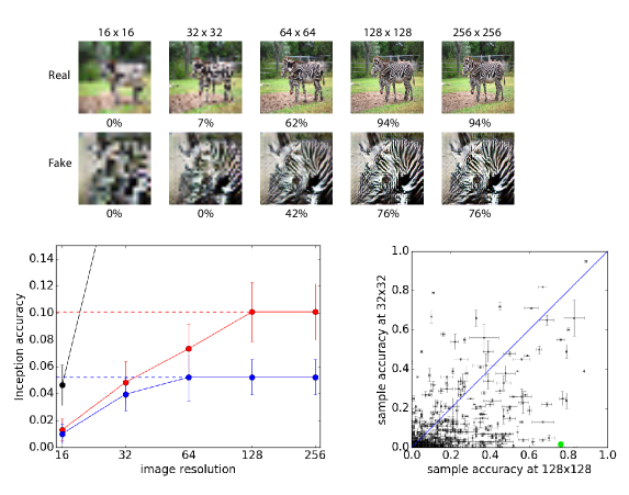
Building a class-conditional image synthesis model necessitates measuring the extent to which synthesized images appear to belong to the intended class. In particular, we would like to know that a high resolution sample is not just a naive resizing of a low resolution sample. Consider a simple experiment: pretend there exists a model that synthesizes $32\times 32$ images. One can trivially increase the resolution of synthesized images by performing bilinear interpolation. This would yield higher resolution images, but these images would just be blurry versions of the low resolution images that are not discriminable. Hence, the goal of an image synthesis model is not simply to produce high resolution images, but to produce high resolution images that are more discriminable than low resolution images.

To measure discriminability, we feed synthesized images to a pre-trained Inception network (Szegedy et al., 2015) and report the fraction of the samples for which the Inception network assigned the correct label. We calculate this accuracy measure on a series of real and synthesized images which have had their spatial resolution artificially decreased by bilinear interpolation (Figure 2, top panels). Note that as the spatial resolution is decreased, the accuracy decreases - indicating that resulting images contain less class information (Figure 2, scores below top panels). We summarized this finding across all 1000 ImageNet classes for the ImageNet training data (black), a $128\times 128$ resolution AC-GAN (red) and a $64\times 64$ resolution AC-GAN (blue) in Figure 2 (bottom, left). The black curve (clipped) provides an upper-bound on the discriminability of real images.

The goal of this analysis is to show that synthesizing higher resolution images leads to increased discriminability. The $128\times 128$ model achieves an accuracy of 10.1% $\pm$ 2.0% versus 7.0% $\pm$ 2.0% with samples resized to $64\times 64$ and 5.0% $\pm$ 2.0% with samples resized to $32\times 32$. In other words, downsizing the outputs of the AC-GAN to $32\times 32$ and $64\times 64$ decreases visual discriminability by 50% and 38% respectively. Furthermore, 84.4% of the ImageNet classes have higher accuracy at $128\times 128$ than at $32\times 32$ (Figure 2, bottom left).

We performed the same analysis on an AC-GAN trained to $64\times 64$ spatial resolution. This model achieved less discriminability than a $128\times 128$ AC-GAN model. Accuracies from the $64\times 64$ model plateau at a $64\times 64$ spatial resolution consistent with previous results. Finally, the $64\times 64$ resolution model achieves less discriminability at 64 spatial resolution than the $128\times 128$ model.

To the best of our knowledge, this work is the first that attempts to measure the extent to which an image synthesis model is ‘making use of its given output resolution’, and in fact is the first work to consider the issue at all. We consider this an important contribution, on par with proposing a model that synthesizes images from all 1000 ImageNet classes. We note that the proposed method can be applied to any image synthesis model for which a measure of ‘sample quality’ can be constructed. In fact, this method (broadly defined) can be applied to any type of synthesis model, as long as there is an easily computable notion of sample quality and some method for ‘reducing resolution’. In particular, we expect that a similar procecure can be carried out for audio synthesis.

4.2 Measuring the Diversity of Generated Images

An image synthesis model is not very interesting if it only outputs one image. Indeed, a well-known failure mode of GANs is that the generator will collapse and output a single prototype that maximally fools the discriminator (Goodfellow et al., 2014; Salimans et al., 2016). A class-conditional model of images is not very interesting if it only outputs one image per class. The Inception accuracy can not measure whether a model has collapsed. A model that simply memorized one example from each ImageNet class would do very well by this metric. Thus, we seek a complementary metric to explicitly evaluate the intra-class perceptual diversity of samples generated by the AC-GAN.

Several methods exist for quantitatively evaluating image similarity by attempting to predict human perceptual similarity judgements. The most successful of these is multi-scale structural similarity (MS-SSIM) (Wang et al., 2004b; Ma et al., 2016). MS-SSIM is a multi-scale variant of a well-characterized perceptual similarity metric that attempts to discount aspects of an image that are not important for human perception (Wang et al., 2004a). MS-SSIM values range between 0.0 and 1.0; higher MS-SSIM values correspond to perceptually more similar images.

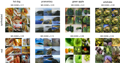
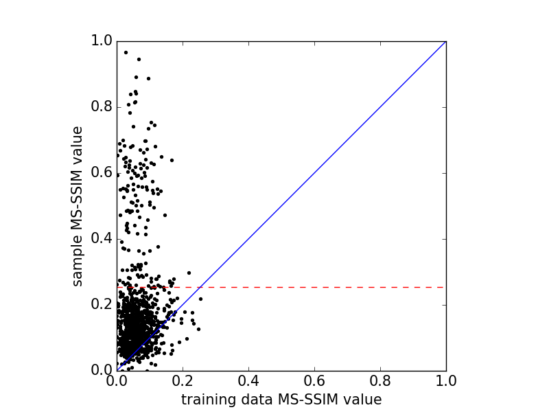
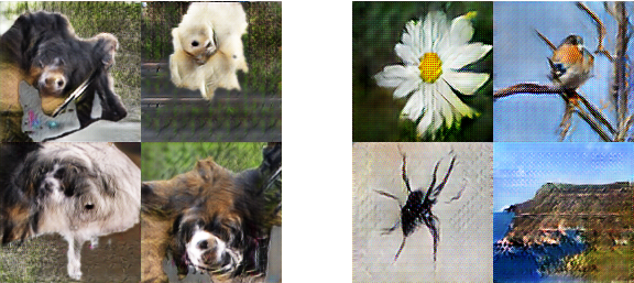
As a proxy for image diversity, we measure the MS-SSIM scores between 100 randomly chosen pairs of images within a given class. Samples from classes that have higher diversity result in lower mean MS-SSIM scores (Figure 3, left columns); samples from classes with lower diversity have higher mean MS-SSIM scores (Figure 3, right columns). Training images from the ImageNet training data contain a variety of mean MS-SSIM scores across the classes indicating the variability of image diversity in ImageNet classes (Figure 4, x-axis). Note that the highest mean MS-SSIM score (indicating the least variability) is 0.25 for the training data.

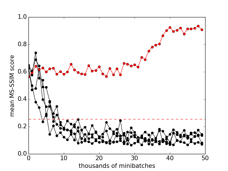
We calculate the mean MS-SSIM score for all 1000 ImageNet classes generated by the AC-GAN model. We track this value during training to identify whether the generator has collapsed (Figure 5, red curve). We also employ this metric to compare the diversity of the training images to the samples from the GAN model after training has completed. Figure 4 plots the mean MS-SSIM values for image samples and training data broken up by class. The blue line is the line of equality. Out of the 1000 classes, we find that 847 have mean sample MS-SSIM scores below that of the maximum MS-SSIM for the training data. In other words, 84.7% of classes have sample variability that exceeds that of the least variable class from the ImageNet training data.

There are two points related to the MS-SSIM metric and our use of it that merit extra attention. The first point is that we are ‘abusing’ the metric: it was originally intended to be used for measuring the quality of image compression algorithms using a reference ‘original image’. We instead use it on two potentially unrelated images. We believe that this is acceptable for the following reasons: First: visual inspection seems to indicate that the metric makes sense - pairs with higher MS-SSIM do seem more similar than pairs with lower MS-SSIM. Second: we restrict comparisons to images synthesized using the same class label. This restricts use of MS-SSIM to situations more similar to those in which it is typically used (it is not important which image is the reference). Third: the metric is not ‘saturated’ for our use-case. If most scores were around 0, then we would be more concerned about the applicability of MS-SSIM. Finally: The fact that training data achieves more variability by this metric (as expected) is itself evidence that the metric is working as intended.

The second point is that the MS-SSIM metric is not intended as a proxy for the entropy of the generator distribution in pixel space, but as a measure of perceptual diversity of the outputs. The entropy of the generator output distribution is hard to compute and pairwise MS-SSIM scores would not be a good proxy. Even if it were easy to compute, we argue that it would still be useful to have a separate measure of perceptual diversity. To see why, consider that the generator entropy will be sensitive to trivial changes in contrast as well as changes in the semantic content of the outputs. In many applications, we don’t care about this contribution to the entropy, and it is useful to consider measures that attempt to ignore changes to an image that we consider ‘perceptually meaningless’, hence the use of MS-SSIM.

Figure 3: Examples of different MS-SSIM scores. The top and bottom rows contain AC-GAN samples and training data, respectively.

Figure 4: Comparison of the mean MS-SSIM scores between pairs of images within a given class for ImageNet training data and samples from the GAN (blue line is equality). The horizontal red line marks the maximum MS-SSIM value (for training data) across all ImageNet classes. Each point is an individual class. The mean score across the training data and the samples was 0.05 and 0.18 respectively. The mean standard deviation of scores across the training data and the samples was 0.06 and 0.08 respectively. Scores below the red line (84.7% of classes) arise from classes where GAN training largely succeeded.

Figure 5: Intra-class MS-SSIM for selected ImageNet classes throughout a training run. Classes that successfully train (black lines) tend to have decreasing mean MS-SSIM scores. Classes for which the generator ‘collapses’ (red line) will have increasing mean MS-SSIM scores.

4.3 Generated Images are both Diverse and Discriminable

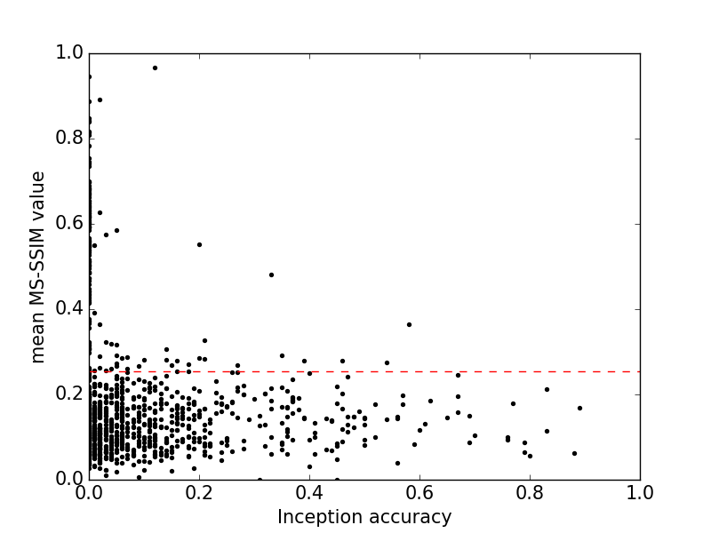
We have presented quantitative metrics demonstrating that AC-GAN samples may be diverse and discriminable but we have yet to examine how these metrics interact. Figure 6 shows the joint distribution of Inception accuracies and MS-SSIM scores across all classes. Inception accuracy and MS-SSIM are anti-correlated ($r^{2}=-0.16$). In fact, 74% of the classes with low diversity (MS-SSIM $\geq 0.25$) contain Inception accuracies $\leq 1\%$. Conversely, 78% of classes with high diversity (MS-SSIM $<0.25$) have Inception accuracies that exceed 1%. In comparison, the Inception-v3 model achieves 78.8% accuracy on average across all 1000 classes (Szegedy et al., 2015). A fraction of the classes AC-GAN samples reach this level of accuracy. This indicates opportunity for future image synthesis models.

These results suggest that GANs that drop modes are most likely to produce low quality images. This stands in contrast to a popular hypothesis about GANs, which is that they achieve high sample quality at the expense of variability. We hope that these findings can help structure further investigation into the reasons for differing sample quality between GANs and other image synthesis models.

Figure 6: Inception accuracy vs MS-SSIM for all 1000 ImageNet classes ($r^{2}=-0.16$). Each data point represents the mean MS-SSIM value for samples from one class. As in Figure 4, the red line marks the maximum MS-SSIM value (for training data) across all ImageNet classes. Samples from AC-GAN models do not achieve variability at the expense of discriminability.

4.4 Comparison to Previous Results

Previous quantitative results for image synthesis models trained on ImageNet are reported in terms of log-likelihood (van den Oord et al., 2016a, b). Log-likelihood is a coarse and potentially inaccurate measure of sample quality (Theis et al., 2015). Instead we compare with previous state-of-the-art results on CIFAR-10 using a lower spatial resolution ($32\times 32$). Following the procedure in (Salimans et al., 2016), we compute the Inception score for 50000 samples from an AC-GAN with resolution ($32\times 32$), split into 10 groups at random. We also compute the Inception score for 25000 extra samples, split into 5 groups at random. We select the best model based on the first score and report the second score. Performing a grid search across 27 hyperparameter configurations, we are able to achieve a score of 8.25 $\pm$ 0.07 compared to state of the art 8.09 $\pm$ 0.07 (Salimans et al., 2016). Moreover, we accomplish this without employing any of the new techniques introduced in that work (i.e. virtual batch normalization, minibatch discrimination, and label smoothing).

This provides additional evidence that AC-GANs are effective even without the benefit of class splitting. See Figure 7 for a qualitative comparison of samples from an AC-GAN and samples from the model in (Salimans et al., 2016).

Figure 7: Samples generated from the ImageNet dataset. (Left) Samples generated from the model in (Salimans et al., 2016). (Right) Randomly chosen samples generated from an AC-GAN. AC-GAN samples possess global coherence absent from the samples of the earlier model.

4.5 Searching for Signatures of Overfitting

One possibility that must be investigated is that the AC-GAN has overfit on the training data. As a first check that the network does not memorize the training data, we identify the nearest neighbors of image samples in the training data measured by L1 distance in pixel space (Figure 8). The nearest neighbors from the training data do not resemble the corresponding samples. This provides evidence that the AC-GAN is not merely memorizing the training data.

Figure 8: Nearest neighbor analysis. (Top) Samples from a single ImageNet class. (Bottom) Corresponding nearest neighbor (L1 distance) in training data for each sample.

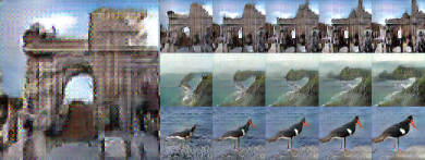
A more sophisticated method for understanding the degree of overfitting in a model is to explore that model’s latent space by interpolation. In an overfit model one might observe discrete transitions in the interpolated images and regions in latent space that do not correspond to meaningful images (Bengio et al., 2012; Radford et al., 2015; Dinh et al., 2016). Figure 9 (Top) highlights interpolations in the latent space between several image samples. Notably, the generator learned that certain combinations of dimensions correspond to semantically meaningful features (e.g. size of the arch, length of a bird’s beak) and there are no discrete transitions or ‘holes’ in the latent space.

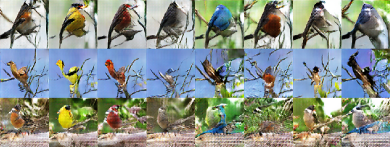
A second method for exploring the latent space of the AC-GAN is to exploit the structure of the model. The AC-GAN factorizes its representation into class information and a class-independent latent representation $z$. Sampling the AC-GAN with $z$ fixed but altering the class label corresponds to generating samples with the same ‘style’ across multiple classes (Kingma et al., 2014). Figure 9 (Bottom) shows samples from 8 bird classes. Elements of the same row have the same $z$. Although the class changes for each column, elements of the global structure (e.g. position, layout, background) are preserved, indicating that AC-GAN can represent certain types of ‘compositionality’.

Figure 9: (Top) Latent space interpolations for selected ImageNet classes. Left-most and right-columns show three pairs of image samples - each pair from a distinct class. Intermediate columns highlight linear interpolations in the latent space between these three pairs of images. (Bottom) Class-independent information contains global structure about the synthesized image. Each column is a distinct bird class while each row corresponds to a fixed latent code $z$.

4.6 Measuring the Effect of Class Splits on Image Sample Quality.

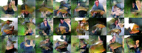
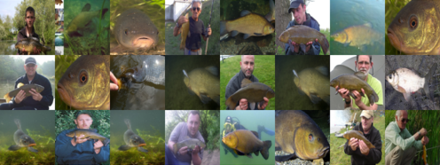
Class conditional image synthesis affords the opportunity to divide up a dataset based on image label. In our final model we divide 1000 ImageNet classes across 100 AC-GAN models. In this section we describe experiments that highlight the benefit of cutting down the diversity of classes for training an AC-GAN. We employed an ordering of the labels and divided it into contiguous groups of 10. This ordering can be seen in the following section, where we display samples from all 1000 classes. Two aspects of the split merit discussion: the number of classes per split and the intra-split diversity. We find that training a fixed model on more classes harms the model’s ability to produce compelling samples (Figure 10). Performance on larger splits can be improved by giving the model more parameters. However, using a small split is not sufficient to achieve good performance. We were unable to train a GAN (Goodfellow et al., 2014) to converge reliably even for a split size of 1. This raises the question of whether it is easier to train a model on a diverse set of classes than on a similar set of classes: We were unable to find conclusive evidence that the selection of classes in a split significantly affects sample quality.

Figure 10: Mean pairwise MS-SSIM values for 10 ImageNet classes plotted against the number of ImageNet classes used during training. We fix everything except the number of classes trained on, using values from 10 to 100. We only report the MS-SSIM values for the first 10 classes to keep the scores comparable. MS-SSIM quickly goes above 0.25 (the red line) as the class count increases. These scores were computed using 9 random restarts per class count, using the same number of training steps for each model. Since we have observed that generators do not recover from the collapse phase, the use of a fixed number of training steps seems justified in this case.

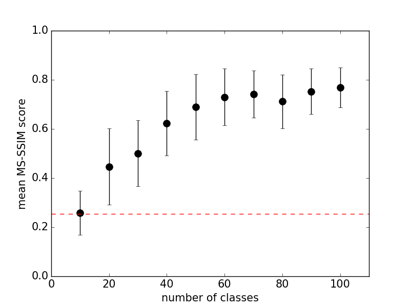
We don’t have a hypothesis about what causes this sensitivity to class count that is well-supported experimentally. We can only note that, since the failure case that occurs when the class count is increased is ‘generator collapse’, it seems plausible that general methods for addressing ‘generator collapse’ could also address this sensitivity.

4.7 Samples from all 1000 ImageNet Classes

We also generate 10 samples from each of the 1000 ImageNet classes, hosted here. As far as we are aware, no other image synthesis work has included a similar analysis.

5 Discussion

This work introduced the AC-GAN architecture and demonstrated that AC-GANs can generate globally coherent ImageNet samples. We provided a new quantitative metric for image discriminability as a function of spatial resolution. Using this metric we demonstrated that our samples are more discriminable than those from a model that generates lower resolution images and performs a naive resize operation. We also analyzed the diversity of our samples with respect to the training data and provided some evidence that the image samples from the majority of classes are comparable in diversity to ImageNet data.

Several directions exist for building upon this work. Much work needs to be done to improve the visual discriminability of the $128\times 128$ resolution model. Although some synthesized image classes exhibit high Inception accuracies, the average Inception accuracy of the model ($10.1\%\pm 2.0\%$) is still far below real training data at 81%. One immediate opportunity for addressing this is to augment the discriminator with a pre-trained model to perform additional supervised tasks (e.g. image segmentation, (Ronneberger et al., 2015)).

Improving the reliability of GAN training is an ongoing research topic. Only 84.7% of the ImageNet classes exhibited diversity comparable to real training data. Training stability was vastly aided by dividing up 1000 ImageNet classes across 100 AC-GAN models. Building a single model that could generate samples from all 1000 classes would be an important step forward.

Image synthesis models provide a unique opportunity for performing semi-supervised learning: these models build a rich prior over natural image statistics that can be leveraged by classifiers to improve predictions on datasets for which few labels exist. The AC-GAN model can perform semi-supervised learning by ignoring the component of the loss arising from class labels when a label is unavailable for a given training image. Interestingly, prior work suggests that achieving good sample quality might be independent of success in semi-supervised learning (Salimans et al., 2016).

Appendix A Hyperparameters

We summarize hyperparameters used for the ImageNet model in Table 1 and for the CIFAR-10 model in Table 2.

Operation	Kernel	Strides	Feature maps	BN?	Dropout	Nonlinearity
$G_{x}(z)$ – $110\times 1\times 1$ input
Linear	N/A	N/A	$768$	$\times$	0.0	ReLU
Transposed Convolution	$5\times 5$	$2\times 2$	$384$	$\surd$	0.0	ReLU
Transposed Convolution	$5\times 5$	$2\times 2$	$256$	$\surd$	0.0	ReLU
Transposed Convolution	$5\times 5$	$2\times 2$	$192$	$\surd$	0.0	ReLU
Transposed Convolution	$5\times 5$	$2\times 2$	$3$	$\times$	0.0	Tanh
$D(x)$ – $128\times 128\times 3$ input
Convolution	$3\times 3$	$2\times 2$	$16$	$\times$	0.5	Leaky ReLU
Convolution	$3\times 3$	$1\times 1$	$32$	$\surd$	0.5	Leaky ReLU
Convolution	$3\times 3$	$2\times 2$	$64$	$\surd$	0.5	Leaky ReLU
Convolution	$3\times 3$	$1\times 1$	$128$	$\surd$	0.5	Leaky ReLU
Convolution	$3\times 3$	$2\times 2$	$256$	$\surd$	0.5	Leaky ReLU
Convolution	$3\times 3$	$1\times 1$	$512$	$\surd$	0.5	Leaky ReLU
Linear	N/A	N/A	$11$	$\times$	0.0	Soft-Sigmoid
Optimizer	Adam ($\alpha=0.0002$, $\beta_{1}=0.5$, $\beta_{2}=0.999$)
Batch size	100
Iterations	50000
Leaky ReLU slope	0.2
Weight, bias initialization	Isotropic gaussian ($\mu=0$, $\sigma=0.02$), Constant($0$)

Table 1: ImageNet hyperparameters. A Soft-Sigmoid refers to an operation over $K+1$ output units where we apply a Softmax activation to $K$ of the units and a Sigmoid activation to the remaining unit. We also use activation noise in the discriminator as suggested in (Salimans et al., 2016).

Operation	Kernel	Strides	Feature maps	BN?	Dropout	Nonlinearity
$G_{x}(z)$ – $110\times 1\times 1$ input
Linear	N/A	N/A	$384$	$\times$	0.0	ReLU
Transposed Convolution	$5\times 5$	$2\times 2$	$192$	$\surd$	0.0	ReLU
Transposed Convolution	$5\times 5$	$2\times 2$	$96$	$\surd$	0.0	ReLU
Transposed Convolution	$5\times 5$	$2\times 2$	$3$	$\times$	0.0	Tanh
$D(x)$ – $32\times 32\times 3$ input
Convolution	$3\times 3$	$2\times 2$	$16$	$\times$	0.5	Leaky ReLU
Convolution	$3\times 3$	$1\times 1$	$32$	$\surd$	0.5	Leaky ReLU
Convolution	$3\times 3$	$2\times 2$	$64$	$\surd$	0.5	Leaky ReLU
Convolution	$3\times 3$	$1\times 1$	$128$	$\surd$	0.5	Leaky ReLU
Convolution	$3\times 3$	$2\times 2$	$256$	$\surd$	0.5	Leaky ReLU
Convolution	$3\times 3$	$1\times 1$	$512$	$\surd$	0.5	Leaky ReLU
Linear	N/A	N/A	$11$	$\times$	0.0	Soft-Sigmoid
Generator Optimizer	Adam ($\alpha=[0.0001,0.0002,0.0003]$, $\beta_{1}=0.5$, $\beta_{2}=0.999$)
Discriminator Optimizer	Adam ($\alpha=[0.0001,0.0002,0.0003]$, $\beta_{1}=0.5$, $\beta_{2}=0.999$)
Batch size	100
Iterations	50000
Leaky ReLU slope	0.2
Activation noise standard deviation	$[0,0.1,0.2]$
Weight, bias initialization	Isotropic gaussian ($\mu=0$, $\sigma=0.02$), Constant($0$)

Table 2: CIFAR-10 hyperparameters. When a list is given for a hyperparameter it means that we performed a grid search using the values in the list. For each set of hyperparameters, a single AC-GAN was trained on the whole CIFAR-10 dataset. For each AC-GAN that was trained, we split up the samples into groups so that we could give some sense of the variance of the Inception Score. To the best of our knowledge, this is identical to the analysis performed in (Salimans et al., 2016).

References

- Ballé et al. (2015) Ballé, Johannes, Laparra, Valero, and Simoncelli, Eero P. Density modeling of images using a generalized normalization transformation. CoRR, abs/1511.06281, 2015. URL http://arxiv.org/abs/1511.06281.
- Bengio et al. (2012) Bengio, Yoshua, Mesnil, Grégoire, Dauphin, Yann, and Rifai, Salah. Better mixing via deep representations. CoRR, abs/1207.4404, 2012. URL http://arxiv.org/abs/1207.4404.
- Blundell et al. (2016) Blundell, C., Uria, B., Pritzel, A., Li, Y., Ruderman, A., Leibo, J. Z, Rae, J., Wierstra, D., and Hassabis, D. Model-Free Episodic Control. ArXiv e-prints, June 2016.
- Chen et al. (2016) Chen, X., Duan, Y., Houthooft, R., Schulman, J., Sutskever, I., and Abbeel, P. InfoGAN: Interpretable Representation Learning by Information Maximizing Generative Adversarial Nets. ArXiv e-prints, June 2016.
- Denton et al. (2015) Denton, Emily L., Chintala, Soumith, Szlam, Arthur, and Fergus, Robert. Deep generative image models using a laplacian pyramid of adversarial networks. CoRR, abs/1506.05751, 2015. URL http://arxiv.org/abs/1506.05751.
- Dinh et al. (2016) Dinh, Laurent, Sohl-Dickstein, Jascha, and Bengio, Samy. Density estimation using real NVP. CoRR, abs/1605.08803, 2016. URL http://arxiv.org/abs/1605.08803.
- Donahue et al. (2016) Donahue, J., Krähenbühl, P., and Darrell, T. Adversarial Feature Learning. ArXiv e-prints, May 2016.
- Dumoulin et al. (2016) Dumoulin, V., Belghazi, I., Poole, B., Lamb, A., Arjovsky, M., Mastropietro, O., and Courville, A. Adversarially Learned Inference. ArXiv e-prints, June 2016.
- Goodfellow et al. (2014) Goodfellow, I. J., Pouget-Abadie, J., Mirza, M., Xu, B., Warde-Farley, D., Ozair, S., Courville, A., and Bengio, Y. Generative Adversarial Networks. ArXiv e-prints, June 2014.
- Kingma & Welling (2013) Kingma, D. P and Welling, M. Auto-Encoding Variational Bayes. ArXiv e-prints, December 2013.
- Kingma et al. (2014) Kingma, Diederik P., Rezende, Danilo Jimenez, Mohamed, Shakir, and Welling, Max. Semi-supervised learning with deep generative models. CoRR, abs/1406.5298, 2014. URL http://arxiv.org/abs/1406.5298.
- Kingma et al. (2016) Kingma, Diederik P., Salimans, Tim, and Welling, Max. Improving variational inference with inverse autoregressive flow. CoRR, abs/1606.04934, 2016. URL http://arxiv.org/abs/1606.04934.
- Ledig et al. (2016) Ledig, C., Theis, L., Huszar, F., Caballero, J., Aitken, A., Tejani, A., Totz, J., Wang, Z., and Shi, W. Photo-Realistic Single Image Super-Resolution Using a Generative Adversarial Network. ArXiv e-prints, September 2016.
- Ma et al. (2016) Ma, Kede, Wu, Qingbo, Wang, Zhou, Duanmu, Zhengfang, Yong, Hongwei, Li, Hongliang, and Zhang, Lei. Group mad competition - a new methodology to compare objective image quality models. In The IEEE Conference on Computer Vision and Pattern Recognition (CVPR), June 2016.
- Maas et al. (2013) Maas, Andrew, Hannun, Awni, and Ng, Andrew. Rectifier nonlinearities improve neural network acoustic models. In Proceedings of The 33rd International Conference on Machine Learning, 2013.
- Mirza & Osindero (2014) Mirza, Mehdi and Osindero, Simon. Conditional generative adversarial nets. CoRR, abs/1411.1784, 2014. URL http://arxiv.org/abs/1411.1784.
- Mohamed & Lakshminarayanan (2016) Mohamed, Shakir and Lakshminarayanan, Balaji. Learning in implicit generative models. arXiv preprint arXiv:1610.03483, 2016.
- Nguyen et al. (2016) Nguyen, Anh Mai, Dosovitskiy, Alexey, Yosinski, Jason, Brox, Thomas, and Clune, Jeff. Synthesizing the preferred inputs for neurons in neural networks via deep generator networks. CoRR, abs/1605.09304, 2016. URL http://arxiv.org/abs/1605.09304.
- Odena (2016) Odena, A. Semi-Supervised Learning with Generative Adversarial Networks. ArXiv e-prints, June 2016.
- Odena et al. (2016) Odena, Augustus, Dumoulin, Vincent, and Olah, Chris. Deconvolution and checkerboard artifacts. http://distill.pub/2016/deconv-checkerboard/, 2016.
- Radford et al. (2015) Radford, Alec, Metz, Luke, and Chintala, Soumith. Unsupervised representation learning with deep convolutional generative adversarial networks. CoRR, abs/1511.06434, 2015. URL http://arxiv.org/abs/1511.06434.
- Ramsundar et al. (2016) Ramsundar, Bharath, Kearnes, Steven, Riley, Patrick, Webster, Dale, Konerding, David, and Pande, Vijay. Massively multitask networks for drug discovery. In Proceedings of The 33rd International Conference on Machine Learning, 2016.
- Reed et al. (2016a) Reed, Scott, Akata, Zeynep, Mohan, Santosh, Tenka, Samuel, Schiele, Bernt, and Lee, Honglak. Learning what and where to draw. arXiv preprint arXiv:1610.02454, 2016a.
- Reed et al. (2016b) Reed, Scott, Akata, Zeynep, Yan, Xinchen, Logeswaran, Lajanugen, Schiele, Bernt, and Lee, Honglak. Generative adversarial text-to-image synthesis. In Proceedings of The 33rd International Conference on Machine Learning, 2016b.
- Rezende & Mohamed (2015) Rezende, D. and Mohamed, S. Variational Inference with Normalizing Flows. ArXiv e-prints, May 2015.
- Rezende et al. (2014) Rezende, D., Mohamed, S., and Wierstra, D. Stochastic Backpropagation and Approximate Inference in Deep Generative Models. ArXiv e-prints, January 2014.
- Ronneberger et al. (2015) Ronneberger, Olaf, Fischer, Philipp, and Brox, Thomas. U-net: Convolutional networks for biomedical image segmentation. CoRR, abs/1505.04597, 2015. URL http://arxiv.org/abs/1505.04597.
- Russakovsky et al. (2015) Russakovsky, Olga, Deng, Jia, Su, Hao, Krause, Jonathan, Satheesh, Sanjeev, Ma, Sean, Huang, Zhiheng, Karpathy, Andrej, Khosla, Aditya, Bernstein, Michael, Berg, Alexander C., and Fei-Fei, Li. ImageNet Large Scale Visual Recognition Challenge. International Journal of Computer Vision (IJCV), 115(3):211–252, 2015. doi: 10.1007/s11263-015-0816-y.
- Salimans et al. (2016) Salimans, T., Goodfellow, I., Zaremba, W., Cheung, V., Radford, A., and Chen, X. Improved Techniques for Training GANs. ArXiv e-prints, June 2016.
- Simoncelli & Olshausen (2001) Simoncelli, Eero and Olshausen, Bruno. Natural image statistics and neural representation. Annual Review of Neuroscience, 24:1193–1216, 2001.
- Springenberg (2015) Springenberg, J. T. Unsupervised and Semi-supervised Learning with Categorical Generative Adversarial Networks. ArXiv e-prints, November 2015.
- Sutskever et al. (2014) Sutskever, Ilya, Vinyals, Oriol, and V., Le Quoc. Sequence to sequence learning with neural networks. In Neural Information Processing Systems, 2014.
- Szegedy et al. (2014) Szegedy, Christian, Liu, Wei, Jia, Yangqing, Sermanet, Pierre, Reed, Scott E., Anguelov, Dragomir, Erhan, Dumitru, Vanhoucke, Vincent, and Rabinovich, Andrew. Going deeper with convolutions. CoRR, abs/1409.4842, 2014. URL http://arxiv.org/abs/1409.4842.
- Szegedy et al. (2015) Szegedy, Christian, Vanhoucke, Vincent, Ioffe, Sergey, Shlens, Jonathon, and Wojna, Zbigniew. Rethinking the inception architecture for computer vision. CoRR, abs/1512.00567, 2015. URL http://arxiv.org/abs/1512.00567.
- Theis et al. (2015) Theis, L., van den Oord, A., and Bethge, M. A note on the evaluation of generative models. ArXiv e-prints, November 2015.
- Toderici et al. (2016) Toderici, George, Vincent, Damien, Johnston, Nick, Hwang, Sung Jin, Minnen, David, Shor, Joel, and Covell, Michele. Full resolution image compression with recurrent neural networks. CoRR, abs/1608.05148, 2016. URL http://arxiv.org/abs/1608.05148.
- Uehara et al. (2016) Uehara, M., Sato, I., Suzuki, M., Nakayama, K., and Matsuo, Y. Generative Adversarial Nets from a Density Ratio Estimation Perspective. ArXiv e-prints, October 2016.
- van den Oord et al. (2016a) van den Oord, Aäron, Kalchbrenner, Nal, and Kavukcuoglu, Koray. Pixel recurrent neural networks. CoRR, abs/1601.06759, 2016a. URL http://arxiv.org/abs/1601.06759.
- van den Oord et al. (2016b) van den Oord, Aäron, Kalchbrenner, Nal, Vinyals, Oriol, Espeholt, Lasse, Graves, Alex, and Kavukcuoglu, Koray. Conditional image generation with pixelcnn decoders. CoRR, abs/1606.05328, 2016b. URL http://arxiv.org/abs/1606.05328.
- Wang et al. (2004a) Wang, Zhou, Bovik, Alan C, Sheikh, Hamid R, and Simoncelli, Eero P. Image quality assessment: from error visibility to structural similarity. IEEE transactions on image processing, 13(4):600–612, 2004a.
- Wang et al. (2004b) Wang, Zhou, Simoncelli, Eero P, and Bovik, Alan C. Multiscale structural similarity for image quality assessment. In Signals, Systems and Computers, 2004. Conference Record of the Thirty-Seventh Asilomar Conference on, volume 2, pp. 1398–1402. Ieee, 2004b.