Through the Haze: a Non-Convex Approach to
Blind Gain Calibration for Linear Random Sensing Models

Valerio Cambareri and Laurent Jacques VC and LJ are with Image and Signal Processing Group (ISPGroup), ICTEAM/ELEN, Université catholique de Louvain (UCL). E-mail: laurent.jacques@uclouvain.be, valerio.cambareri@uclouvain.be. The authors are funded by the Belgian F.R.S.-FNRS. Part of this study is funded by the project AlterSense (MIS-FNRS).
Abstract

Computational sensing strategies often suffer from calibration errors in the physical implementation of their ideal sensing models. Such uncertainties are typically addressed by using multiple, accurately chosen training signals to recover the missing information on the sensing model, an approach that can be resource-consuming and cumbersome. Conversely, blind calibration does not employ any training signal, but corresponds to a bilinear inverse problem whose algorithmic solution is an open issue. We here address blind calibration as a non-convex problem for linear random sensing models, in which we aim to recover an unknown signal from its projections on sub-Gaussian random vectors, each subject to an unknown positive multiplicative factor (or gain). To solve this optimisation problem we resort to projected gradient descent starting from a suitable, carefully chosen initialisation point. An analysis of this algorithm allows us to show that it converges to the exact solution provided a sample complexity requirement is met, i.e., relating convergence to the amount of information collected during the sensing process. Interestingly, we show that this requirement grows linearly (up to log\log factors) in the number of unknowns of the problem. This sample complexity is found both in absence of prior information, as well as when subspace priors are available for both the signal and gains, allowing a further reduction of the number of observations required for our recovery guarantees to hold. Moreover, in the presence of noise we show how our descent algorithm yields a solution whose accuracy degrades gracefully with the amount of noise affecting the measurements. Finally, we present some numerical experiments in an imaging context, where our algorithm allows for a simple solution to blind calibration of the gains in a sensor array.

Keywords: Blind calibration, non-convex optimisation, sample complexity, bilinear inverse problems.
2000 Math Subject Classification: 94A15, 94A20, 90C26,15A29.

1 Introduction

The problem of recovering an unknown signal measured or transmitted by means of an inaccurate sensing model is of crucial importance for modern sensing strategies relying on the solution of inverse problems. In such problems, exact prior information on the sensing model is paramount to accurately reconstruct the original signal. Compressed Sensing (CS) [1] has emerged as a powerful framework to design new sensing strategies employing sub-Gaussian random matrix ensembles given their remarkable properties (see, e.g.,  [2]). However, model errors inevitably affect its physical implementation and can significantly degrade signal recovery, as first studied by Herman and Strohmer [3]. In particular, such model errors may arise from physical causes such as unknown convolution kernels [4, 5, 6] affecting the measurements; unknown attenuations or gains on the latter coefficients, e.g., pixel response non-uniformity [7] or fixed-pattern noise in imaging systems; complex-valued (i.e., gain and phase) errors in sensor arrays [8, 9, 10].

Assuming such errors remain stationary throughout the sensing process, the use of linear random operators in CS does suggest that repeating the acquisition, i.e., taking several snapshots under new independent draws of a random sensing operator could suffice to diversify the measurements and extract the information required to learn both the unknown signal and the model error. In this paper we adopt this general principle to achieve the blind calibration of sensor gains, that is the joint recovery of an unknown signal and some unknown multiplicative factors (i.e., the gains) not accounted for in the assumed sensing model. Our method is inspired by recent results on fast, provably convergent algorithms for phase retrieval [11, 12, 13] and entails solving a non-convex problem by means of a descent algorithm that is presented below. Most importantly, this paper is concerned with finding the conditions under which the convergence of our algorithm to the exact solution is guaranteed, i.e., a bound on the number of measurements m𝑚m and snapshots p𝑝p collected during the sensing process, along with some mild requirements on the entity of the gains. Hence, our main concern will be to establish a sample complexity, i.e., a lower bound on the total amount of observations collected during the sensing process: we will see that this bound must fulfil mp=𝒪((m+n)log2(m(p+n)))𝑚𝑝𝒪𝑚𝑛superscript2𝑚𝑝𝑛mp={\mathcal{O}}\big{(}(m+n)\log^{2}(m(p+n))\big{)} with n𝑛n the dimensionality of the signal and m𝑚m that of the gains, up to a condition on n=𝒪(logmp)𝑛𝒪𝑚𝑝n={\mathcal{O}}(\log mp). This methodology allows for provably exact blind calibration under some mild hypotheses on the gains for the sensing models we describe in the next section.

1.1 Sensing Models

Our paper focuses on blind calibration for systems based on linear random sensing modalities. As described hereafter, we will assume that each observation is obtained by projection on a random vector 𝒂n𝒂superscript𝑛\boldsymbol{a}\in\mathbb{R}^{n} that is composed of n𝑛n independent and identically distributed (i.i.d.) components drawn as aji.i.d.Xsubscriptsimilar-toi.i.d.subscript𝑎𝑗𝑋a_{j}\sim_{\rm\textrm{i.i.d.}}X, j[n]𝑗delimited-[]𝑛j\in[n], where X𝑋X is a centred sub-Gaussian random variable (r.v.) having unit variance and sub-Gaussian norm α>0𝛼0\alpha>0 (for a thorough introduction to such concepts, we refer the reader to [14, Section 5.2.5]). We recall that Gaussian, Bernoulli or bounded r.v.’s all pertain to the class of sub-Gaussian r.v.’s for some finite α𝛼\alpha. In this context, the sensing models tackled by this paper are defined as follows111The notation used in this section anticipates the one that is fully explained in Sec. 1.4..

Definition 1.1 (Uncalibrated Multi-Snapshot Sensing Model).

We define uncalibrated multi-snapshot sensing model any instance of

𝒚l=diag(𝒈)𝑨l𝒙=[g1(𝒂1,l𝒙),,gm(𝒂m,l𝒙)],l[p],formulae-sequencesubscript𝒚𝑙diag𝒈subscript𝑨𝑙𝒙superscriptsubscript𝑔1superscriptsubscript𝒂1𝑙top𝒙subscript𝑔𝑚superscriptsubscript𝒂𝑚𝑙top𝒙top𝑙delimited-[]𝑝{\boldsymbol{y}}_{l}\ =\ \operatorname{{diag}}({\boldsymbol{g}}){\boldsymbol{A}}_{l}{\boldsymbol{x}}\ =\ \big{[}g_{1}(\boldsymbol{a}_{1,l}^{\top}{\boldsymbol{x}}),\ \cdots,g_{m}(\boldsymbol{a}_{m,l}^{\top}{\boldsymbol{x}})\big{]}^{\top},\quad l\in[p], (1.1)

where the m𝑚m-dimensional measurement vector 𝐲lmsubscript𝐲𝑙superscript𝑚{\boldsymbol{y}}_{l}\in\mathbb{R}^{m} is the l𝑙l-th snapshot associated to the l𝑙l-th random sensing matrix 𝐀l=(𝐚1,l,,𝐚m,l)m×nsubscript𝐀𝑙superscriptsubscript𝐚1𝑙subscript𝐚𝑚𝑙topsuperscript𝑚𝑛{\boldsymbol{A}}_{l}=(\boldsymbol{a}_{1,l},\,\cdots,\boldsymbol{a}_{m,l})^{\top}\in\mathbb{R}^{m\times n} with 𝐚i,li.i.d.𝐚subscriptsimilar-toi.i.d.subscript𝐚𝑖𝑙𝐚\boldsymbol{a}_{i,l}\sim_{\textrm{i.i.d.}}\boldsymbol{a}, i.e., all the matrices {𝐀l:l[p]}conditional-setsubscript𝐀𝑙𝑙delimited-[]𝑝\{{\boldsymbol{A}}_{l}:l\in[p]\} are i.i.d.. The vector 𝐱n𝐱superscript𝑛{\boldsymbol{x}}\in\mathbb{R}^{n} is an unknown, unstructured signal and 𝐠+m𝐠subscriptsuperscript𝑚{\boldsymbol{g}}\in\mathbb{R}^{m}_{+} are unknown, positive and bounded gains, both quantities remaining fixed throughout the p𝑝p snapshots entailed by the sensing process.

The noisy case of this model is given hereafter by considering additive and bounded disturbances, i.e.,

𝒚l=diag(𝒈)𝑨l𝒙+𝝂l,l[p],formulae-sequencesubscript𝒚𝑙diag𝒈subscript𝑨𝑙𝒙subscript𝝂𝑙𝑙delimited-[]𝑝{\boldsymbol{y}}_{l}=\operatorname{{diag}}({\boldsymbol{g}})\,{\boldsymbol{A}}_{l}{\boldsymbol{x}}+\boldsymbol{\nu}_{l},\ l\in[p], (1.2)

where the noise vectors 𝛎lmsubscript𝛎𝑙superscript𝑚\boldsymbol{\nu}_{l}\in\mathbb{R}^{m}, l[p]𝑙delimited-[]𝑝l\in[p] are collected in a matrix 𝐍m×p𝐍superscript𝑚𝑝\boldsymbol{N}\in\mathbb{R}^{m\times p} with σ1mp𝐍F<𝜎1𝑚𝑝subscriptnorm𝐍𝐹\sigma\coloneqq\textstyle\tfrac{1}{\sqrt{mp}}\|\boldsymbol{N}\|_{F}<\infty.

These bilinear sensing models are related to computational sensing applications in which unknown 𝒈𝒈{\boldsymbol{g}} are associated to positive gains in a sensor array, while p𝑝p random matrix instances can be applied on a source 𝒙𝒙{\boldsymbol{x}} by means of a suitable, typically programmable medium. In particular, the setup in (1.1) matches compressive imaging configurations [15, 16, 17, 6, 18] with an important difference in that the absence of a priori structure on (𝒙,𝒈)𝒙𝒈({\boldsymbol{x}},{\boldsymbol{g}}) in Def. 1.1 implies an over-Nyquist sampling regime with respect to n𝑛ni.e., exceeding the number of unknowns as mpn+m𝑚𝑝𝑛𝑚mp\geq n+m. When the effect of 𝒈𝒈{\boldsymbol{g}} is critical, i.e., assuming diag(𝒈)𝑰mdiag𝒈subscript𝑰𝑚\operatorname{{diag}}({\boldsymbol{g}})\approx\boldsymbol{I}_{m} would lead to an inaccurate recovery of 𝒙𝒙{\boldsymbol{x}}, finding solutions to (1.1) in (𝒙,𝒈)𝒙𝒈({\boldsymbol{x}},{\boldsymbol{g}}) justifies a possibly over-Nyquist sampling regime (that is mp>n𝑚𝑝𝑛mp>n) as long as both quantities can be recovered accurately (e.g., as an on-line calibration modality). To show that more efficient sampling regimes in mp𝑚𝑝mp are possible we now introduce known subspace priors, paving the way to actual blind calibration for CS.

Definition 1.2 (Uncalibrated Multi-Snapshot Sensing Model with Subspace Priors.).

Given two subspaces msuperscript𝑚\mathcal{B}\subset\mathbb{R}^{m} and 𝒵n𝒵superscript𝑛\mathcal{Z}\subset\mathbb{R}^{n}, of dimension hdimmdimension𝑚h\coloneqq\dim\mathcal{B}\leq m and kdim𝒵n𝑘dimension𝒵𝑛k\coloneqq\dim\mathcal{Z}\leq n, with orthonormal bases 𝐁m×h𝐁superscript𝑚\boldsymbol{B}\in\mathbb{R}^{m\times h} and 𝐙n×k𝐙superscript𝑛𝑘{\boldsymbol{Z}}\in\mathbb{R}^{n\times k}, respectively, we define uncalibrated sensing model with subspace priors any instance of (1.1) (or of (1.2), in the presence of noise) where 𝐱𝐙𝐳𝒵𝐱𝐙𝐳𝒵{\boldsymbol{x}}\coloneqq{\boldsymbol{Z}}{\boldsymbol{z}}\in\mathcal{Z} for 𝐳k𝐳superscript𝑘{\boldsymbol{z}}\in\mathbb{R}^{k}, and 𝐠𝐁𝐛𝐠𝐁𝐛{\boldsymbol{g}}\coloneqq{\boldsymbol{B}}{\boldsymbol{b}} for 𝐛h𝐛superscript\boldsymbol{b}\in\mathbb{R}^{h}.

This known subspace prior is specially relevant for the signal domain, since such models are not necessarily present in the gain domain (e.g., the gains can be fully random due to the nature of the device that captures the measurements). When compared to sparse models for the signal and gains (i.e., when either 𝒙𝒙{\boldsymbol{x}} or 𝒈𝒈{\boldsymbol{g}} lie in a union of low-dimensional canonical subspaces) Def. 1.2 amounts to knowing the support of their respective sparse representations. Thus, while enforcing actual sparsity priors in the signal domain seems numerically feasible [19] we leave its theoretical analysis for a future communication given the depth of the additional considerations required to prove it.

Note that our analysis of both previous bilinear sensing models will exploit the fact that the deviation between the gains 𝒈𝒈\boldsymbol{g} and 𝟏msubscript1𝑚\boldsymbol{1}_{m} (up to a scaling factor) is significant, but not too large and, in fact, bounded in subscript\ell_{\infty}-norm. Depending on which model is considered, this assumption is first detailed in Sec. 2, then specified in the known subspace case of Sec. 4.

It is finally worth noting that the above sensing models are strongly related and could be generalised to blind deconvolution by modifying (1.1), i.e., by letting the measurements

𝒚l=(𝑭m1𝒈)𝑨l𝒙=𝑭m1diag(𝒈)𝑭m𝑨l𝒙,l[p],formulae-sequencesubscript𝒚𝑙superscriptsubscript𝑭𝑚1𝒈subscript𝑨𝑙𝒙superscriptsubscript𝑭𝑚1diag𝒈subscript𝑭𝑚subscript𝑨𝑙𝒙𝑙delimited-[]𝑝{\boldsymbol{y}}_{l}=({\boldsymbol{F}}_{m}^{-1}{\boldsymbol{g}})\circledast{\boldsymbol{A}}_{l}{\boldsymbol{x}}={\boldsymbol{F}}_{m}^{-1}\operatorname{{diag}}({\boldsymbol{g}}){\boldsymbol{F}_{m}}\,{\boldsymbol{A}}_{l}{\boldsymbol{x}},\ l\in[p], (1.3)

with 𝑭msubscript𝑭𝑚\boldsymbol{F}_{m} being the m𝑚m-dimensional discrete Fourier transform and \circledast the circular convolution operator. However, assessing the performances of our algorithm for this case with generally complex-valued (𝒙,𝒈)𝒙𝒈({\boldsymbol{x}},{\boldsymbol{g}}) is beyond the scope of this contribution.

Before proceeding, let us state a minor working hypothesis on the interaction of the input vector 𝒙𝒙\boldsymbol{x} with the distribution X𝑋X controlling the random vectors {𝒂i,l}subscript𝒂𝑖𝑙\{\boldsymbol{a}_{i,l}\} in the very special case where 𝔼X4=1𝔼superscript𝑋41\mathbb{E}X^{4}=1, e.g., if X𝑋X is a Bernoulli r.v..

Hypothesis (Bernoulli Restriction).

If 𝔼X4=1𝔼superscript𝑋41\mathbb{E}X^{4}=1, we will additionally assume n>1𝑛1n>1 and that there exists some constant c>0𝑐0c>0 such that

𝒙^441cn,superscriptsubscriptnorm^𝒙441𝑐𝑛\|\hat{\boldsymbol{x}}\|_{4}^{4}\leq 1-\tfrac{c}{n},

with 𝐱^=𝐱𝐱2^𝐱𝐱superscriptnorm𝐱2\hat{\boldsymbol{x}}=\tfrac{\boldsymbol{x}}{\|\boldsymbol{x}\|^{2}}.

This hypothesis is purely technical and is likely an artifact of our proofs222Moreover, this restriction could be relaxed to assuming 𝒙^441cnssuperscriptsubscriptnorm^𝒙441𝑐superscript𝑛𝑠\|\hat{\boldsymbol{x}}\|_{4}^{4}\leq 1-\tfrac{c}{n^{s}} for any power s>1𝑠1s>1, as this would only change the universal constants appearing in all our results.. Its origin is actually found in the use of a matrix version of Bernstein’s concentration inequality [4, 20, 21] (see Prop. A.3 in App. A) that imposes a non-vanishing matrix variance for the concentrating sum of centred matrices. Our hypothesis is also minor as (i)𝑖(i) by Jensen’s inequality we have 𝔼X4(𝔼X2)2=1𝔼superscript𝑋4superscript𝔼superscript𝑋221\mathbb{E}X^{4}\geq(\mathbb{E}X^{2})^{2}=1, and (ii)𝑖𝑖(ii) when 𝔼X4=1𝔼superscript𝑋41\mathbb{E}X^{4}=1, this just prevents us to take (in this very specific case) vectors lying “too close” to any of the coordinate axes 𝒄𝒄\boldsymbol{c} of nsuperscript𝑛\mathbb{R}^{n}, which are the only unit vectors whose 𝒄44=𝒄4=1superscriptsubscriptnorm𝒄44superscriptnorm𝒄41\|\boldsymbol{c}\|_{4}^{4}=\|\boldsymbol{c}\|^{4}=1. A possible strategy to avoid this restriction could consist in forming a mixture X(1λ)X+λYsimilar-tosuperscript𝑋1𝜆𝑋𝜆𝑌X^{\prime}\sim(1-\lambda)X+\lambda Y of X𝑋X with another arbitrary centred distribution Y𝑌Y with 𝔼Y4>1𝔼superscript𝑌41\mathbb{E}Y^{4}>1, 𝔼Y2=1𝔼superscript𝑌21\mathbb{E}Y^{2}=1 and λ[0,1]𝜆01\lambda\in[0,1]. For instance we could take Y𝒩(0,1)similar-to𝑌𝒩01Y\sim\mathcal{N}(0,1), whose 𝔼Y4=3𝔼superscript𝑌43\mathbb{E}Y^{4}=3. Then, by linearity of the expectation operator with respect to the involved probability density measure, 𝔼X4=(1λ)+λ𝔼Y4>1𝔼superscript𝑋41𝜆𝜆𝔼superscript𝑌41\mathbb{E}X^{\prime 4}=(1-\lambda)+\lambda\mathbb{E}Y^{4}>1, so that for small λ𝜆\lambda the distribution Xsuperscript𝑋X^{\prime} is arbitrarily close to X𝑋X, yet so that the fourth-moment hypothesis above is satisfied.

1.2 Relation to Prior Works

General Literature on Blind Calibration:  Prior approaches to blind calibration of sensor gains include convex or alternating optimisation algorithms [22, 10, 23] as well as message-passing approaches [24]. In more detail, Balzano and Nowak [22] use a signal-domain subspace prior to infer sensor gains in absence of random sensing operators, i.e., in a conventional sampling scheme. This approach is extended by Lipor and Balzano [23] in the presence of errors in the prior. Bilen et al. [10] use a sparse signal model for multiple inputs and solve a convex version of blind calibration for complex-valued gains. This is numerically shown to be successful in achieving blind calibration for CS. The approach of Schülke et al. [24] is based on a generalised approximate message passing framework, therefore taking into account a probabilistic model for the signal and gains. All the former approaches are aided by multiple input signals (e.g.𝒙lsubscript𝒙𝑙{\boldsymbol{x}}_{l}l[p]𝑙delimited-[]𝑝l\in[p]) instead of taking new draws of the sensing operator itself, while there are clear assumptions on the independence of such signals. Moreover, no formal recovery guarantee is given in these works, i.e., no requirement is obtained on the number of measurements required to perform provably exact blind calibration.

We now proceed to a comparison of our setup with three prior contributions that are closer to our aims, i.e., they develop algorithms with exact recovery guarantees (and their required sample complexity) for either blind calibration or blind deconvolution. To do so, we recast our setup as follows. Let us define 𝒘𝟏pp𝒈𝒲mp𝒘tensor-productsubscript1𝑝𝑝𝒈𝒲superscript𝑚𝑝{\boldsymbol{w}}\coloneqq\tfrac{\boldsymbol{1}_{p}}{\sqrt{p}}\otimes{\boldsymbol{g}}\in\mathcal{W}\subset\mathbb{R}^{mp}, with tensor-product\otimes the Kronecker product and 𝒲𝒲\mathcal{W} a subspace, by repeating p𝑝p times the same gains 𝒈𝒈\boldsymbol{g}. Then we collect the snapshots of (1.1) in

𝒚[𝒚1𝒚p]=diag(𝒘)𝑨𝒙,𝑨[𝑨1𝑨p].formulae-sequence𝒚matrixsubscript𝒚1subscript𝒚𝑝diag𝒘𝑨𝒙𝑨matrixsubscript𝑨1subscript𝑨𝑝{\boldsymbol{y}}\coloneqq\begin{bmatrix}{\boldsymbol{y}}_{1}\\ \vdots\\ {\boldsymbol{y}}_{p}\end{bmatrix}=\operatorname{{diag}}({\boldsymbol{w}})\boldsymbol{A}\boldsymbol{x},\ \boldsymbol{A}\coloneqq\begin{bmatrix}{\boldsymbol{A}}_{1}\\ \vdots\\ {\boldsymbol{A}}_{p}\end{bmatrix}. (1.4)

Let us assume 𝒙=𝒁𝒛𝒙𝒁𝒛\boldsymbol{x}=\boldsymbol{Z}\boldsymbol{z} for some known subspace defined by a basis 𝒁n×k𝒁superscript𝑛𝑘\boldsymbol{Z}\in\mathbb{R}^{n\times k}. Depending on whether we are considering Def. 1.1 or Def. 1.2 we will then have either 𝒲{𝟏pp𝒗:𝒗m}𝒲conditional-settensor-productsubscript1𝑝𝑝𝒗𝒗superscript𝑚\mathcal{W}\coloneqq\big{\{}\tfrac{\boldsymbol{1}_{p}}{\sqrt{p}}\otimes\boldsymbol{v}:{\boldsymbol{v}}\in\mathbb{R}^{m}\big{\}} with m=dim𝒲𝑚dimension𝒲m=\dim\mathcal{W}, or 𝒲{(𝟏pp𝑩)𝒗:𝒗h}𝒲conditional-settensor-productsubscript1𝑝𝑝𝑩𝒗𝒗superscript\mathcal{W}\coloneqq\big{\{}(\tfrac{\boldsymbol{1}_{p}}{\sqrt{p}}\otimes\boldsymbol{B})\boldsymbol{v}:{\boldsymbol{v}}\in\mathbb{R}^{h}\big{\}} with h=dim𝒲dimension𝒲h=\dim\mathcal{W} since 𝒈=𝑩𝒃𝒈𝑩𝒃\boldsymbol{g}=\boldsymbol{B}\boldsymbol{b}, 𝑩m×h𝑩superscript𝑚\boldsymbol{B}\in\mathbb{R}^{m\times h}. Moreover, let us briefly introduce the definition of coherence333Note that μmax(𝟏pp𝐁)=mphmaxj[mp]1p(𝟏p𝐁)𝐜j=μmax(𝐁)subscriptμtensor-productsubscript1𝑝𝑝𝐁𝑚𝑝subscript𝑗delimited-[]𝑚𝑝1𝑝normsuperscripttensor-productsubscript1𝑝𝐁topsubscript𝐜𝑗subscriptμ𝐁\upmu_{\max}\big{(}\tfrac{\boldsymbol{1}_{p}}{\sqrt{p}}\otimes\boldsymbol{B}\big{)}=\sqrt{\tfrac{mp}{h}}\max_{j\in[mp]}\textstyle\tfrac{1}{\sqrt{p}}\|({\boldsymbol{1}_{p}}\otimes\boldsymbol{B})^{\top}\boldsymbol{c}_{j}\|=\upmu_{\max}(\boldsymbol{B}). of 𝑩𝑩\boldsymbol{B} as

μmax(𝑩)mhmaxi[m]𝑩𝒄i[1,mh],subscriptμ𝑩𝑚subscript𝑖delimited-[]𝑚normsuperscript𝑩topsubscript𝒄𝑖1𝑚\upmu_{\max}(\boldsymbol{B})\coloneqq\sqrt{\tfrac{m}{h}}\max_{i\in[m]}\|\boldsymbol{B}^{\top}\boldsymbol{c}_{i}\|\in\big{[}1,\sqrt{\tfrac{m}{h}}\big{]},

with 𝒄isubscript𝒄𝑖\boldsymbol{c}_{i} denoting the canonical basis vectors. This quantity frequently appears in related works [4, 9] and shall be explained carefully in Sec. 4. Another recurring quantity that will not return in our analysis and main results is

μpm𝒈𝒈,subscriptμp𝑚subscriptnorm𝒈norm𝒈\upmu_{\rm p}\coloneqq\sqrt{m}\tfrac{\|\boldsymbol{g}\|_{\infty}}{\|\boldsymbol{g}\|},

which measures the peak-to-energy ratio of a specific instance of 𝒈𝒈\boldsymbol{g}. In our developments this will be implicitly bounded as μp<1+ρsubscriptμp1𝜌\upmu_{\rm p}<1+\rho for a value ρ<1𝜌1\rho<1 and will be therefore considered as a constant smaller than 222.

We omit from the following comparison the recent contribution of Ahmed et al. [25], which tackles provably exact recovery for blind deconvolution in a different setup, i.e., when both the signal and gains are sparse (and, due to this assumption, both are required to have such a sparse representation on random bases verifying several conditions).

Ahmed, Recht and Romberg [4]:  The use of a lifting approach for the solution of bilinear inverse problems was first proposed in this fundamental contribution, which addressed the problem of blind deconvolution (see also [5, 6, 26]). As pointed out in (1.3) this sensing model encompasses blind calibration up to taking, in all generality, complex (𝒙,𝒈)𝒙𝒈(\boldsymbol{x},\boldsymbol{g}) due to the application of 𝑭msubscript𝑭𝑚\boldsymbol{F}_{m}. Loosely speaking, Ahmed et al. assume a deterministic, known subspace prior on 𝒈=𝑩𝒃𝒈𝑩𝒃\boldsymbol{g}=\boldsymbol{B}\boldsymbol{b} as we do. However, the random sensing matrix 𝑨𝑨\boldsymbol{A} in (1.4) is assumed i.i.d. Gaussian, whereas we consider i.i.d. sub-Gaussian 𝑨𝑨\boldsymbol{A}. Moreover, no prior is considered on the signal444In Ahmed et al. our signal 𝒙𝒙\boldsymbol{x} is the message 𝒎𝒎\boldsymbol{m} that undergoes encoding by a random matrix 𝑪𝑪\boldsymbol{C}, the latter being equivalent to 𝑨𝑨\boldsymbol{A} in (1.4). 𝒙𝒙\boldsymbol{x}.

To show provably exact recovery, the authors leverage guarantees based on constructing a dual certificate for their lifted, semidefinite (i.e., convex) problem via the so-called “golfing scheme” [27]. The sample complexity required to recover exactly (𝒙,𝒈)𝒙𝒈(\boldsymbol{x},\boldsymbol{g}) in [4, Thm. 1] is then shown to be of the order of mp=𝒪(max{μmax2h,μp2n}log3(mp))𝑚𝑝𝒪subscriptsuperscriptμ2superscriptsubscriptμp2𝑛superscript3𝑚𝑝mp=\mathcal{O}(\max\{\upmu^{2}_{\max}h,\upmu_{\rm p}^{2}\,n\}\log^{3}(mp)). This is equivalent to what we will find in our Thm. 4.1, mp=𝒪((n+μmax2(𝑩)h)log2(m(p+n)))𝑚𝑝𝒪𝑛subscriptsuperscriptμ2𝑩superscript2𝑚𝑝𝑛mp=\mathcal{O}\big{(}(n+\upmu^{2}_{\max}(\boldsymbol{B})h)\log^{2}(m(p+n))\big{)}, if no subspace prior holds on 𝒙𝒙\boldsymbol{x} (i.e.𝒁=𝑰n𝒁subscript𝑰𝑛\boldsymbol{Z}=\boldsymbol{I}_{n}). This equivalence of sample complexities (up to log\log factors), even if obtained using different algorithmic frameworks and in a setup more general than ours, suggests that this rate is somehow intrinsic to this class of bilinear inverse problems.

Ling and Strohmer [9]:  This recent contribution also proposed a lifting approach to jointly recover (𝒙,𝒈)𝒙𝒈({\boldsymbol{x}},{\boldsymbol{g}}) in (1.1), i.e., specifically for blind calibration. The setup of [9] is indeed the closest to the ones analysed in this paper. A first and foremost difference is in that, by letting 𝑨l,l[p]subscript𝑨𝑙𝑙delimited-[]𝑝{\boldsymbol{A}}_{l},l\in[p] be i.i.d. sub-Gaussian random matrices we have partitioned the sensing operator in several independent snapshots, as opposed to a single snapshot in [9]. Moreover, Ling and Strohmer assume that the signal 𝒙𝒙{\boldsymbol{x}} is complex-valued and sparse, while we tackled only known subspace priors. Their vector 𝒘𝒘{\boldsymbol{w}} in (1.4) is also complex-valued and described by a known subspace. Hence, their setup is still more general than the models we address in this paper.

The techniques used in Ling and Strohmer are similar in principle to those of Ahmed, Recht and Romberg: both contributions use lifting and obtain recovery guarantees via the aforementioned golfing scheme. In detail, [9, Thm. 3.1] shows that the solution to (1.4) for i.i.d. Gaussian 𝑨lsubscript𝑨𝑙{\boldsymbol{A}}_{l} can be found with a sample complexity given by [9, (3.15)], that is mp=𝒪(mnlog(mn)log2(mp))𝑚𝑝𝒪𝑚𝑛𝑚𝑛superscript2𝑚𝑝{mp}={\mathcal{O}}(mn\log(mn)\,\log^{2}(mp)) in absence of subspace priors. Otherwise, when such priors are given, this requirement would be mp=𝒪(μmax2(𝑩)hkloghnlog2(mp))𝑚𝑝𝒪subscriptsuperscriptμ2𝑩𝑘𝑛superscript2𝑚𝑝mp={\mathcal{O}}(\upmu^{2}_{\max}(\boldsymbol{B})hk\log hn\,\log^{2}(mp)). Our main results, while less general, will otherwise show that mp𝑚𝑝mp == 𝒪((k+μmax2(𝑩)h)\mathcal{O}\big{(}(k+\upmu^{2}_{\max}(\boldsymbol{B})h) log2(m(p+n)))\log^{2}(m(p+n))\big{)} when n=𝒪(logmp)𝑛𝒪𝑚𝑝n={\mathcal{O}}(\log mp).

From a numerical standpoint the main limitation of the lifting approach of [9] is computational, i.e., a semidefinite problem must be solved to recover a large-scale rank-one matrix 𝒙𝒈𝒙superscript𝒈top{\boldsymbol{x}}{\boldsymbol{g}}^{\top}. This approach becomes computationally inefficient and unaffordable quite rapidly as m𝑚m and n𝑛n in the uncalibrated sensing model exceed a few hundreds. This is the main reason why we have undertaken the challenge of devising a non-convex optimisation framework for blind calibration, drawing mainly from the principles and concepts presented by Candès et al. [28] in the context of phase retrieval. Just like a non-convex approach to phase retrieval based on a simple gradient descent algorithm with a careful initialisation strategy improved upon the former work of Candès et al. [29], we found that the same type of approach can lead to highly efficient blind calibration in the presence of unknown gains, that is computationally affordable for very high-dimensional signals and gains.

Li, Ling, Strohmer and Wei [20]:   Between our first short communication [30] and the finalisation of this paper a remarkable contribution from Li et al. [20] showed that a non-convex approach to blind deconvolution is indeed capable of provably exact recovery, in a framework that would be applicable to blind calibration. Both our work and Li et al. were inspired by the same non-convex approach of Candès et al. [11]. Thus, there are indeed some similarities between our paper and Li et al. since, loosely speaking, the general methodology both papers rely on is (i)𝑖(i) the definition of an initialisation for a descent algorithm, and (ii)𝑖𝑖(ii) the verification of some mild regularity conditions on the gradient of a non-convex objective in a neighbourhood defined by the initialiser, so that a suitable gradient descent algorithm converges to the exact solution. Moreover, both Li et al. and our work consider known subspace priors on the signal and the gains, so our sensing model (when suitably recast as in (1.4)) is essentially equivalent to theirs.

There are however some important differences worth pointing out. Our approach uses 𝑨𝑨\boldsymbol{A} comprised of p𝑝p independent snapshots with i.i.d. sub-Gaussian sensing matrices. Li et al. tackle the case of a complex Gaussian sensing matrix 𝑨𝑨\boldsymbol{A}. In our case, we will bound a priori the perturbation between the uncalibrated and true sensing model, i.e., we will have a condition on 𝒈𝟏msubscriptnorm𝒈subscript1𝑚\|\boldsymbol{g}-\boldsymbol{1}_{m}\|_{\infty} for 𝒈𝟏m=msuperscript𝒈topsubscript1𝑚𝑚\boldsymbol{g}^{\top}\boldsymbol{1}_{m}=m. Li et al. instead assume a prior on the aforementioned peak-to-energy ratio μpsubscriptμp\upmu_{\rm p}, as well as a small μmax(𝑩)subscriptμ𝑩\upmu_{\max}(\boldsymbol{B}). Our initialisation is a simple back-projection in the signal domain, which also uses the boundedness of 𝒈𝟏msubscriptnorm𝒈subscript1𝑚\|\boldsymbol{g}-\boldsymbol{1}_{m}\|_{\infty} and the use of p𝑝p snapshots. Li et al. use a spectral initialisation closer to what was done in [11], followed by an optimisation problem that enforces a constraint on μpsubscriptμp\upmu_{\rm p}. Given such priors, these must then be enforced by our respective algorithms: in our case, we carry out a projected gradient descent that minimises a non-convex objective with a convex constraint, with the projector affecting only the gain domain (so the gains verify the bound on 𝒈𝟏msubscriptnorm𝒈subscript1𝑚\|\boldsymbol{g}-\boldsymbol{1}_{m}\|_{\infty}). The method of Li et al. uses instead a regularised objective function without constraints, which however must enforce their condition on μpsubscriptμp\upmu_{\rm p}.

In terms of sample complexity, our results range from a worst-case setting in which no subspace model is assumed to the case of known subspace priors, where we require mp=𝒪((k+μmax2(𝑩)h)log2(m(p+n)))𝑚𝑝𝒪𝑘subscriptsuperscriptμ2𝑩superscript2𝑚𝑝𝑛mp=\mathcal{O}\big{(}(k+\upmu^{2}_{\max}(\boldsymbol{B})h)\log^{2}(m(p+n))\big{)}. In Li et al. the obtained sample complexity, by a comparison through (1.4), would be mp=𝒪(max{μmax2(𝑩)h,μp2k}log2(mp))𝑚𝑝𝒪subscriptsuperscriptμ2𝑩superscriptsubscriptμp2𝑘superscript2𝑚𝑝mp={\mathcal{O}}(\max\{\upmu^{2}_{\max}(\boldsymbol{B})h,\upmu_{\rm p}^{2}k\}\log^{2}(mp)) under a careful account of μmax(𝑩)subscriptμ𝑩\upmu_{\max}(\boldsymbol{B}). Thus, while the problem setup of Li et al. is quite general, their sample complexity obtained in [20, Thm. 3.2] is substantially the same and indeed close to that of Ahmed et al.. In fact, we stress that the sample complexities we obtain and the former ones are substantially similar and given by the intrinsic properties of this bilinear inverse problem. Hence, we conclude that our work is essentially alternative to Li et al., as it applies to sub-Gaussian sensing matrices and uses some specific conditions related to blind calibration of sensor gains, while admittedly not addressing the more general case of (1.3). Moreover, the theory we leverage to prove our main results is slightly simpler.

1.3 Main Contributions and Outline

The main contribution of this paper is in showing that for all the uncalibrated sensing models specified in Def. 1.1 and Def. 1.2 it is possible to prove that a very simple and efficient projected gradient descent algorithm promoting the Euclidean data fidelity to the measurements actually converges (under very mild hypotheses) to the exact solution, which verifies (1.1) up to an unrecoverable scaling factor. This descent algorithm strongly relies on an initialisation strategy that is, in fact, a simple back-projection of the measurements. This provides an unbiased estimate of the signal-domain solution under the hypotheses of Def. 1.1, and puts the first iteration of our descent algorithm in a neighbourhood of the global minimiser. Once this neighbourhood can be shown to be sufficiently small, and provided that the perturbations with respect to the available information on the sensing model are also small (in particular, far from the loss of information corresponding to any zero gain gi=0subscript𝑔𝑖0g_{i}=0) the behaviour of the gradients used in the iterates of our algorithms is close to its expectation as the sample complexity mp𝑚𝑝mp grows, i.e., as a consequence of the concentration of measure phenomenon. This allows us to find the conditions on mp𝑚𝑝mp that ensure convergence to the exact solution, depending on which sensing model is chosen. In particular, our substantial contribution is in showing that this sample complexity grows as mp=𝒪((n+m)log2(m(p+n)))𝑚𝑝𝒪𝑛𝑚superscript2𝑚𝑝𝑛mp=\mathcal{O}\big{(}(n+m)\log^{2}(m(p+n))\big{)}, i.e., only proportionally to the number of unknowns n+m𝑛𝑚n+m of this problem (up to log\log factors). Moreover, when this number of unknowns is reduced by the use of known subspace priors, i.e., as in Def. 1.2, we show that this complexity only needs to grow as mp=𝒪((k+μmax2h)log2(m(p+n)))𝑚𝑝𝒪𝑘subscriptsuperscriptμ2superscript2𝑚𝑝𝑛mp=\mathcal{O}\big{(}(k+\upmu^{2}_{\max}h)\log^{2}(m(p+n))\big{)}, i.e., again linearly (up to log\log factors and the effect of a coherence parameter μmax[1,mh]subscriptμ1𝑚\upmu_{\max}\in\big{[}1,\sqrt{\tfrac{m}{h}}\big{]}) in the number of unknowns k𝑘k and hh.

Note that a short communication that partially overlaps with this work was published by the authors [30]. It is here improved and expanded with revised proofs, results on the stability of the proposed approach in the presence of noise, and the possibility of introducing known subspaces to model the signal and gain domains with the aim of reducing the sample complexity of this problem, i.e., minimising the amount of required snapshots in Def. 1.2 when more information on the unknowns is available.

The rest of this paper is structured as follows. In Sec. 2 we formalise the blind calibration problem in its non-convex form and in absence of priors. We explore some of its geometric properties, both in expectation as well as for a finite number of snapshots. There, we define the main notions of distance and neighbourhood used in proving the properties of this problem, and we see that some local convexity properties do hold in expectation. Our main algorithm is then introduced in Sec. 3 and followed by its convergence guarantees in absence of priors, which actually enables a simple understanding of our main results. In Sec. 4 we discuss a modification of our algorithm in the case of known subspace priors for 𝒙𝒙{\boldsymbol{x}} and 𝒈𝒈{\boldsymbol{g}}. We show how the anticipated sample complexity improvement is achieved using such prior models and discuss the convergence of a descent algorithm that enforces them properly. Most importantly, the proofs for this case are the cornerstones of this paper, and serve to prove the somewhat simpler results we obtained in absence of priors and advocated in [30]. In Sec. 5 a noise stability analysis is then proposed to show how the accuracy of the solution is affected by the presence of bounded noise in the measurements. In Sec. 6 we provide numerical evidence on our algorithm’s empirical phase transition, highlighting the regime that grants exact recovery of the signal and gains. This is followed by an empirical discussion of the descent algorithm’s step size update, and by an assessment of the stability of our algorithm in the presence of noise. All three cases are carried out in absence of priors, i.e., in a worst-case setup.  A practical application of our method to a realistic computational sensing context, both in absence and in presence of known subspace priors, concludes the experiments carried out in this paper. The proofs of all mathematical statements and tools used in this paper are reported in the appendices.

1.4 Notation and Conventions

The notation throughout the paper is as follows: vectors and matrices are denoted by boldface lower-case and upper-case letters respectively, e.g.𝒒𝒒\boldsymbol{q} and 𝑸𝑸\boldsymbol{Q}, while scalars and constants are denoted as q𝑞q, Q𝑄Q. The vectors 𝟎qsubscript0𝑞\boldsymbol{0}_{q} and 𝟏qsubscript1𝑞\boldsymbol{1}_{q} indicate a vector of dimension q𝑞q, respectively of all zeros or ones and with size specified in the subscript. The identity matrix of dimension q𝑞q is 𝑰qsubscript𝑰𝑞\boldsymbol{I}_{q}. The rows, columns and entries of a matrix 𝑸𝑸\boldsymbol{Q} will be denoted as 𝑸j,subscript𝑸𝑗\boldsymbol{Q}_{j,\cdot}, 𝑸,jsubscript𝑸𝑗\boldsymbol{Q}_{\cdot,j} and Qijsubscript𝑄𝑖𝑗Q_{ij} respectively. An exception to this rule are the rows of the sensing matrices 𝑨lsubscript𝑨𝑙\boldsymbol{A}_{l}, denoted as 𝒂i,lsuperscriptsubscript𝒂𝑖𝑙top\boldsymbol{a}_{i,l}^{\top} (i.e., as the column vectors 𝒂i,lsubscript𝒂𝑖𝑙\boldsymbol{a}_{i,l}). Sets and operators are generally denoted with calligraphic capital letters, e.g.𝒮𝒮\mathcal{S}, 𝒜𝒜\mathcal{A}. The n𝑛n-variate Gaussian distribution is denoted as 𝒩(𝟎n,𝑰n)𝒩subscript0𝑛subscript𝑰𝑛\mathcal{N}(\boldsymbol{0}_{n},\boldsymbol{I}_{n}), the uniform distribution is 𝒰𝒞subscript𝒰𝒞\mathcal{U}_{\mathcal{C}} over a set 𝒞𝒞\mathcal{C} specified at the argument. The usual big-O notation is indicated by 𝒪𝒪\mathcal{O}. The Kronecker product between vectors of matrices is denoted by tensor-product\otimes. Collections of vectors or matrices can be indexed by single or double subscripts, e.g.𝒂isubscript𝒂𝑖\boldsymbol{a}_{i} or 𝒂i,lsubscript𝒂𝑖𝑙\boldsymbol{a}_{i,l}. For the sake of brevity, we may omit the boundaries of sums that are identical throughout the development: unless otherwise stated, isubscript𝑖\textstyle\sum_{i} denotes i=1msubscriptsuperscript𝑚𝑖1\textstyle\sum^{m}_{i=1}, lsubscript𝑙\textstyle\sum_{l} denotes l=1psubscriptsuperscript𝑝𝑙1\textstyle\sum^{p}_{l=1}, i,lsubscript𝑖𝑙\textstyle\sum_{i,l} denotes i=1ml=1psubscriptsuperscript𝑚𝑖1subscriptsuperscript𝑝𝑙1\textstyle\sum^{m}_{i=1}\textstyle\sum^{p}_{l=1}. For some integer q>0𝑞0q>0, we denote the set [q]{1,,q}delimited-[]𝑞1𝑞[q]\coloneqq\{1,\ldots,q\}. The norms in p(q)subscript𝑝superscript𝑞\ell_{p}(\mathbb{R}^{q}) are denoted as usual with p\|\cdot\|_{p} with =2\|\cdot\|=\|\cdot\|_{2}. The spectral norm of a matrix reads \|\cdot\|, while the Frobenius norm and scalar product are F\|\cdot\|_{F} and ,Fsubscript𝐹\langle\cdot,\cdot\rangle_{F}, respectively. Spheres and balls in p(q)subscript𝑝superscript𝑞\ell_{p}(\mathbb{R}^{q}) will be denoted by 𝕊pq1subscriptsuperscript𝕊𝑞1𝑝\mathbb{S}^{q-1}_{p} and 𝔹pqsubscriptsuperscript𝔹𝑞𝑝{\mathbb{B}}^{q}_{p} respectively. For matrices, we also introduce the Frobenius sphere and ball, defined respectively as 𝕊Fn×m={𝑼n×m:𝑼F=1}superscriptsubscript𝕊𝐹𝑛𝑚conditional-set𝑼superscript𝑛𝑚subscriptnorm𝑼𝐹1\mathbb{S}_{F}^{n\times m}=\{\boldsymbol{U}\in\mathbb{R}^{n\times m}:\|\boldsymbol{U}\|_{F}=1\} and 𝔹Fn×m={𝑼n×m:𝑼F1}superscriptsubscript𝔹𝐹𝑛𝑚conditional-set𝑼superscript𝑛𝑚subscriptnorm𝑼𝐹1\mathbb{B}_{F}^{n\times m}=\{\boldsymbol{U}\in\mathbb{R}^{n\times m}:\|\boldsymbol{U}\|_{F}\leq 1\}. The projection operator on a closed convex set 𝒞𝒞\mathcal{C} is 𝒫𝒞subscript𝒫𝒞{\mathcal{P}}_{\mathcal{C}}, while orthogonal projection on a linear subspace \mathcal{B} is denoted by the projection matrix 𝑷subscript𝑷{\boldsymbol{P}}_{\mathcal{B}}. The symbol i.i.d.subscriptsimilar-toi.i.d.\sim_{\rm\textrm{i.i.d.}} indicates that a collection of random variables (abbreviated as r.v.) or vectors on the left hand side (l.h.s.) of the operator are independent and follow the same distribution given on the right hand side (r.h.s.). The Orlicz norm of a random variable A𝐴A is denoted as Aψqsupr1r1/q𝔼[|A|r]1/r\|A\|_{\psi_{q}}\coloneqq\sup_{r\geq 1}\textstyle r^{-1/q}{\operatorname{{\mathbb{E}}}[|A|^{r}]}^{1/r} with the sub-exponential and sub-Gaussian norms being the cases for q=1𝑞1q=1 and q=2𝑞2q=2 respectively. We will often resort to some constants C,c>0𝐶𝑐0C,c>0, as traditional in the derivation of non-asymptotic results for sub-Gaussian random vectors and matrices. The value of these constants is not relevant and may change from line to line, as long as it does not depend on the problem dimensions. The quantity 𝒗f(,𝒗,)subscriptbold-∇𝒗𝑓𝒗\boldsymbol{\nabla}_{\boldsymbol{v}}f(\ldots,{\boldsymbol{v}},\ldots) denotes the gradient operator with respect to the vector 𝒗𝒗{\boldsymbol{v}} specified in the subscript, as applied on a function f𝑓f. In absence of subscripts, it is the gradient of f𝑓f with respect to all of its components. f𝑓\mathcal{H}f denotes the Hessian matrix of f𝑓f. The set Π+m={𝒗+m, 1m𝒗=m}superscriptsubscriptΠ𝑚formulae-sequence𝒗subscriptsuperscript𝑚subscriptsuperscript1top𝑚𝒗𝑚\Pi_{+}^{m}=\{{\boldsymbol{v}}\in\mathbb{R}^{m}_{+},\,\boldsymbol{1}^{\top}_{m}{\boldsymbol{v}}=m\} denotes the scaled probability simplex. We will also refer to the orthogonal complement 𝟏m{𝒗m:𝟏m𝒗=0}msubscriptsuperscript1perpendicular-to𝑚conditional-set𝒗superscript𝑚superscriptsubscript1𝑚top𝒗0superscript𝑚{{\boldsymbol{1}}^{\perp}_{m}}\coloneqq\{{\boldsymbol{v}}\in\mathbb{R}^{m}:\boldsymbol{1}_{m}^{\top}{\boldsymbol{v}}=0\}\subset\mathbb{R}^{m}. Moreover, when vectors and matrices are projected or lie on the latter subspace they will be denoted with the superscript superscriptperpendicular-to\cdot^{\perp}. The canonical basis vectors of msuperscript𝑚\mathbb{R}^{m} are denoted by 𝒄isubscript𝒄𝑖{\boldsymbol{c}}_{i}, i[m]𝑖delimited-[]𝑚i\in[m]. Their projection on 𝟏msubscriptsuperscript1perpendicular-to𝑚{{\boldsymbol{1}}^{\perp}_{m}} is 𝒄i𝑷𝟏m𝒄isubscriptsuperscript𝒄perpendicular-to𝑖subscript𝑷subscriptsuperscript1perpendicular-to𝑚subscript𝒄𝑖{\boldsymbol{c}}^{\perp}_{i}\coloneqq{\boldsymbol{P}}_{{{\boldsymbol{1}}^{\perp}_{m}}}{\boldsymbol{c}}_{i}. The operator succeeds-or-equals\succeq denotes the Löwner ordering on the convex cone of symmetric positive-semidefinite matrices (if strict, this is denoted as succeeds\succ). The absence of this ordering is denoted as not-succeeds-nor-equals\nsucceq. The restriction of this ordering to test vectors belonging to a set 𝒜𝒜\mathcal{A} is denoted in the subscript, e.g.𝒜subscriptsucceeds𝒜\succ_{\mathcal{A}}. The accent ~~\tilde{\cdot} will denote the noisy version of a quantity at the argument that was previously defined in absence of noise, while the accent ¯¯\bar{\cdot} denotes the estimates attained by an optimisation algorithm. The accent ^^\hat{\cdot} denotes unit vectors obtained from the argument (𝒒^=𝒒𝒒^𝒒𝒒norm𝒒\hat{\boldsymbol{q}}=\tfrac{\boldsymbol{q}}{\|\boldsymbol{q}\|}) or unit matrices with respect to the Frobenius norm (𝑸^=𝑸𝑸F^𝑸𝑸subscriptnorm𝑸𝐹\widehat{\boldsymbol{Q}}=\tfrac{\boldsymbol{Q}}{\|\boldsymbol{Q}\|_{F}}). The superscript ssuperscripts\cdot^{\rm s} denotes a quantity defined to accommodate subspace priors, while the superscript .c.^{\rm c} denotes the complementary of an event.

2 A Non-Convex Approach to Blind Calibration

We now proceed to introduce our main non-convex optimisation problem and its geometric properties, depending on the dimensions of the setup in Def. 1.1.

2.1 The Blind Calibration Problem

The formulation of an inverse problem for (1.1) is quite natural by means of a Euclidean data fidelity objective function f(𝝃,𝜸)12mpl=1pdiag(𝜸)𝑨l𝝃𝒚l2𝑓𝝃𝜸12𝑚𝑝superscriptsubscript𝑙1𝑝superscriptnormdiag𝜸subscript𝑨𝑙𝝃subscript𝒚𝑙2f({\boldsymbol{\xi}},{\boldsymbol{\gamma}})\coloneqq\tfrac{1}{2mp}{\textstyle\sum_{l=1}^{p}\left\|\operatorname{{diag}}({\boldsymbol{\gamma}}){\boldsymbol{A}}_{l}{\boldsymbol{\xi}}-{\boldsymbol{y}}_{l}\right\|^{2}} (this is further expanded in Table 1 for both finite and asymptotic p𝑝p). Since no a priori structure is assumed on the solution (𝒙,𝒈)n×+m𝒙𝒈superscript𝑛subscriptsuperscript𝑚({\boldsymbol{x}},{\boldsymbol{g}})\in\mathbb{R}^{n}\times\mathbb{R}^{m}_{+} for now, let us operate in the overdetermined case mpn+m𝑚𝑝𝑛𝑚mp\geq n+m and solve the optimisation problem

(𝒙¯,𝒈¯)argmin(𝝃,𝜸)n×m12mpl=1pdiag(𝜸)𝑨l𝝃𝒚l2,¯𝒙¯𝒈subscriptargmin𝝃𝜸superscript𝑛superscript𝑚12𝑚𝑝superscriptsubscript𝑙1𝑝superscriptnormdiag𝜸subscript𝑨𝑙𝝃subscript𝒚𝑙2(\bar{{\boldsymbol{x}}},\bar{{\boldsymbol{g}}})\coloneqq{\mathop{\operatorname{{argmin}}}_{({\boldsymbol{\xi}},{\boldsymbol{\gamma}})\in\mathbb{R}^{n}\times\mathbb{R}^{m}}}\tfrac{1}{2mp}{\textstyle\sum_{l=1}^{p}\left\|\operatorname{{diag}}({\boldsymbol{\gamma}}){\boldsymbol{A}}_{l}{\boldsymbol{\xi}}-{\boldsymbol{y}}_{l}\right\|^{2}}, (2.1)

with 𝒚lmsubscript𝒚𝑙superscript𝑚{\boldsymbol{y}}_{l}\in\mathbb{R}^{m}, 𝑨lm×nsubscript𝑨𝑙superscript𝑚𝑛{\boldsymbol{A}}_{l}\in\mathbb{R}^{m\times n}, l[p]𝑙delimited-[]𝑝l\in[p] as in Def. 1.1. To begin with, replacing 𝒚lsubscript𝒚𝑙{\boldsymbol{y}}_{l} by its model (1.1) in (2.1) shows that, in absence of prior information on 𝒙𝒙\boldsymbol{x} or 𝒈𝒈{\boldsymbol{g}}, all points in

𝒳{(𝝃,𝜸)n×m:𝝃=α1𝒙,𝜸=α𝒈,α{0}}𝒳conditional-set𝝃𝜸superscript𝑛superscript𝑚formulae-sequence𝝃superscript𝛼1𝒙formulae-sequence𝜸𝛼𝒈𝛼0\mathcal{X}\coloneqq\{({\boldsymbol{\xi}},{\boldsymbol{\gamma}})\in\mathbb{R}^{n}\times\mathbb{R}^{m}:{\boldsymbol{\xi}}={\alpha}^{-1}{\boldsymbol{x}},\,{\boldsymbol{\gamma}}=\alpha{\boldsymbol{g}},\,\alpha\in\mathbb{R}\setminus\{0\}\}

are global minimisers of f(𝝃,𝜸)𝑓𝝃𝜸f({\boldsymbol{\xi}},{\boldsymbol{\gamma}}) up to an unrecoverable scaling factor α𝛼\alpha. This ambiguity is an inevitable aspect of many bilinear inverse problems that is well recognised in the referenced literature (for a more general theory on the identifiability of this class of problems, we refer the reader to some recent contributions [6, 31, 32]). In most applications this scaling ambiguity is equivalent to ignoring the norm of the original signal and is an acceptable loss of information. Thus, since we also know that 𝒈𝒈\boldsymbol{g} is positive, we could apply a constraint such as 𝜸Π+m{𝒗+m, 1m𝒗=m}𝜸superscriptsubscriptΠ𝑚formulae-sequence𝒗subscriptsuperscript𝑚subscriptsuperscript1top𝑚𝒗𝑚{\boldsymbol{\gamma}}\in\Pi_{+}^{m}\coloneqq\{{\boldsymbol{v}}\in\mathbb{R}^{m}_{+},\,\boldsymbol{1}^{\top}_{m}{\boldsymbol{v}}=m\} in (2.1), which would fix the 1subscript1\ell_{1}-norm of the gain-domain solution. This yields the minimiser (𝒙,𝒈)(𝒈1m𝒙,m𝒈1𝒈)𝒳(n×Π+m)superscript𝒙superscript𝒈subscriptnorm𝒈1𝑚𝒙𝑚subscriptnorm𝒈1𝒈𝒳superscript𝑛superscriptsubscriptΠ𝑚({\boldsymbol{x}}^{\star},{\boldsymbol{g}}^{\star})\coloneqq\big{(}\tfrac{\|{\boldsymbol{g}}\|_{1}}{m}{\boldsymbol{x}},\tfrac{m}{\|{\boldsymbol{g}}\|_{1}}{\boldsymbol{g}}\big{)}\in\mathcal{X}\cap(\mathbb{R}^{n}\times\Pi_{+}^{m}), i.e., scaled by α=m𝒈1𝛼𝑚subscriptnorm𝒈1\alpha=\tfrac{m}{\|{\boldsymbol{g}}\|_{1}}. In other words, (2.1) has only one non-trivial global minimiser over 𝒳(n×Π+m)𝒳superscript𝑛superscriptsubscriptΠ𝑚\mathcal{X}\cap(\mathbb{R}^{n}\times\Pi_{+}^{m}) and at least one in n×Π+msuperscript𝑛superscriptsubscriptΠ𝑚\mathbb{R}^{n}\times\Pi_{+}^{m} (this minimiser’s uniqueness can only be shown in a neighbourhood and shall be proved afterwards). As a result, since 𝒈+m𝒈subscriptsuperscript𝑚{\boldsymbol{g}}\in\mathbb{R}^{m}_{+} in Def. 1.1 is positive, bounded and close to unity, the gain-domain solution of (2.1) with the additional constraint 𝜸Π+m𝜸superscriptsubscriptΠ𝑚\boldsymbol{\gamma}\in\Pi_{+}^{m} will actually be

𝒈𝒢ρΠ+m,𝒢ρ𝟏m+𝟏mρ𝔹m,ρ<1,formulae-sequencesuperscript𝒈subscript𝒢𝜌subscriptsuperscriptΠ𝑚formulae-sequencesubscript𝒢𝜌subscript1𝑚subscriptsuperscript1perpendicular-to𝑚𝜌subscriptsuperscript𝔹𝑚𝜌1{\boldsymbol{g}}^{\star}\in{\mathcal{G}}_{\rho}\subset\Pi^{m}_{+},\,{\mathcal{G}}_{\rho}\coloneqq\boldsymbol{1}_{m}+{{\boldsymbol{1}}^{\perp}_{m}}\cap\rho\,{\mathbb{B}}^{m}_{\infty},\,\rho<1,

for a maximum deviation ρ𝒈𝟏m𝜌subscriptnormsuperscript𝒈subscript1𝑚\rho\geq\|{\boldsymbol{g}}^{\star}-\boldsymbol{1}_{m}\|_{\infty} which we assume known at least for what concerns the analysis of the proposed algorithms. Thus, under the constraint 𝜸𝒢ρ𝜸subscript𝒢𝜌\boldsymbol{\gamma}\in{\mathcal{G}}_{\rho} we can specify that 𝒈𝟏m+𝒆superscript𝒈subscript1𝑚𝒆{\boldsymbol{g}}^{\star}\coloneqq\boldsymbol{1}_{m}+{\boldsymbol{e}} for 𝒆𝟏mρ𝔹m𝒆subscriptsuperscript1perpendicular-to𝑚𝜌subscriptsuperscript𝔹𝑚{\boldsymbol{e}}\in{{\boldsymbol{1}}^{\perp}_{m}}\cap\rho\,{\mathbb{B}}^{m}_{\infty} as well as 𝜸𝟏m+𝜺𝜸subscript1𝑚𝜺{\boldsymbol{\gamma}}\coloneqq\boldsymbol{1}_{m}+\boldsymbol{\varepsilon} for 𝜺𝟏mρ𝔹m𝜺subscriptsuperscript1perpendicular-to𝑚𝜌subscriptsuperscript𝔹𝑚\boldsymbol{\varepsilon}\in{{\boldsymbol{1}}^{\perp}_{m}}\cap\rho\,{\mathbb{B}}^{m}_{\infty}. With these simple considerations obtained by construction from Def. 1.1 we arrive to the following problem, that is simply (2.1) with 𝜸𝒢ρΠ+m𝜸subscript𝒢𝜌superscriptsubscriptΠ𝑚{\boldsymbol{\gamma}}\in{\mathcal{G}}_{\rho}\subset\Pi_{+}^{m}.

Definition 2.1 (Non-convex Blind Calibration Problem).

We define non-convex blind calibration the optimisation problem

(𝒙¯,𝒈¯)argmin(𝝃,𝜸)n×𝒢ρ12mpl=1pdiag(𝜸)𝑨l𝝃𝒚l2,¯𝒙¯𝒈subscriptargmin𝝃𝜸superscript𝑛subscript𝒢𝜌12𝑚𝑝superscriptsubscript𝑙1𝑝superscriptnormdiag𝜸subscript𝑨𝑙𝝃subscript𝒚𝑙2(\bar{{\boldsymbol{x}}},\bar{{\boldsymbol{g}}})\coloneqq{\mathop{\operatorname{{argmin}}}_{({\boldsymbol{\xi}},{\boldsymbol{\gamma}})\in\mathbb{R}^{n}\times\mathcal{G}_{\rho}}}\tfrac{1}{2mp}{\textstyle\sum_{l=1}^{p}\left\|\operatorname{{diag}}({\boldsymbol{\gamma}}){\boldsymbol{A}}_{l}{\boldsymbol{\xi}}-{\boldsymbol{y}}_{l}\right\|^{2}}, (2.2)

where

𝒢ρ{𝒗m:𝒗𝟏m+𝟏mρ𝔹m},subscript𝒢𝜌conditional-set𝒗superscript𝑚𝒗subscript1𝑚subscriptsuperscript1perpendicular-to𝑚𝜌subscriptsuperscript𝔹𝑚{\mathcal{G}}_{\rho}\coloneqq\big{\{}\boldsymbol{v}\in\mathbb{R}^{m}:\boldsymbol{v}\in\boldsymbol{1}_{m}+{{\boldsymbol{1}}^{\perp}_{m}}\cap\rho\,{\mathbb{B}}^{m}_{\infty}\big{\}}, (2.3)

given ρ<1𝜌1\rho<1, 𝐲lmsubscript𝐲𝑙superscript𝑚{\boldsymbol{y}}_{l}\in\mathbb{R}^{m}, 𝐀lm×nsubscript𝐀𝑙superscript𝑚𝑛{\boldsymbol{A}}_{l}\in\mathbb{R}^{m\times n}, l[p]𝑙delimited-[]𝑝l\in[p] as in Def. 1.1.

For finite p𝑝p, we remark that the minimiser (𝒙,𝒈)superscript𝒙superscript𝒈(\boldsymbol{x}^{\star},\boldsymbol{g}^{\star}) of (2.2) is still not necessarily the only one: to begin with, we would have to ensure that 𝒦l=1pKer𝑨l={𝟎n}𝒦superscriptsubscript𝑙1𝑝Kersubscript𝑨𝑙subscript0𝑛\mathcal{K}\coloneqq\bigcap\limits_{l=1}^{p}{\rm Ker}{\boldsymbol{A}}_{l}=\{\boldsymbol{0}_{n}\} which, however, holds with probability 111 if mp>n𝑚𝑝𝑛mp>n and 𝑨lsubscript𝑨𝑙{\boldsymbol{A}}_{l} is an i.i.d. sub-Gaussian random matrix. Hence, taking the number of measurements mpn+m𝑚𝑝𝑛𝑚mp\geq n+m to be sufficiently large reduces, but does not generally exclude the possibility of stationary points in the domain of (2.2). This possibility will only be cleared out later in Cor. 3.1, where we will be able to show that the magnitude of the gradient of (2.2) is non-null in a neighbourhood of the global minimiser (𝒙,𝒈)superscript𝒙superscript𝒈({\boldsymbol{x}}^{\star},{\boldsymbol{g}}^{\star}). However, since f(𝝃,𝜸)𝑓𝝃𝜸f({\boldsymbol{\xi}},{\boldsymbol{\gamma}}) is non-convex (as further detailed below), devising an algorithm to find such a minimiser is non-trivial and requires a better understanding of the geometry of this problem, starting from its discussion in the next section.

Hereafter, we shall simplify the notation (𝒙,𝒈)superscript𝒙superscript𝒈(\boldsymbol{x}^{\star},\boldsymbol{g}^{\star}) to (𝒙,𝒈)𝒙𝒈(\boldsymbol{x},\boldsymbol{g}), i.e., in all generality, we can assume 𝒈𝒈\boldsymbol{g} is directly normalized so that 𝒈1=msubscriptnorm𝒈1𝑚\|\boldsymbol{g}\|_{1}=m, i.e., so that it lies in 𝒢ρΠ+msubscript𝒢𝜌subscriptsuperscriptΠ𝑚\mathcal{G}_{\rho}\subset\Pi^{m}_{+}.

2.2 The Geometry of Blind Calibration

2.2.1 Preliminaries

We now expand the objective function f(𝝃,𝜸)𝑓𝝃𝜸f({\boldsymbol{\xi}},{\boldsymbol{\gamma}}) of (2.2), its gradient f(𝝃,𝜸)=[(𝝃f(𝝃,𝜸))(𝜸f(𝝃,𝜸))]bold-∇𝑓𝝃𝜸superscriptmatrixsuperscriptsubscriptbold-∇𝝃𝑓𝝃𝜸topsuperscriptsubscriptbold-∇𝜸𝑓𝝃𝜸toptop\boldsymbol{\nabla}f({\boldsymbol{\xi}},{\boldsymbol{\gamma}})=\begin{bmatrix}(\boldsymbol{\nabla}_{\boldsymbol{\xi}}f({\boldsymbol{\xi}},{\boldsymbol{\gamma}}))^{\top}&(\boldsymbol{\nabla}_{\boldsymbol{\gamma}}f({\boldsymbol{\xi}},{\boldsymbol{\gamma}}))^{\top}\end{bmatrix}^{\top} and Hessian matrix f(𝝃,𝜸)𝑓𝝃𝜸\mathcal{H}f({\boldsymbol{\xi}},{\boldsymbol{\gamma}}) as reported in Table 1 in two useful forms for this paper (the matrix form is more convenient for the implementation, the explicit form as a function of the sensing vectors 𝒂i,lsubscript𝒂𝑖𝑙\boldsymbol{a}_{i,l} is analogue to that used in the proofs of our main results). There, we confirm that f(𝝃,𝜸)𝑓𝝃𝜸f({\boldsymbol{\xi}},{\boldsymbol{\gamma}}) is generally non-convex. In fact, as noted in [26] it is bilinear and biconvex, i.e., convex once either 𝝃𝝃{\boldsymbol{\xi}} or 𝜸𝜸{\boldsymbol{\gamma}} are fixed in (2.2) (this suggests that an alternating minimisation with sufficiently many samples mp𝑚𝑝mp could also converge, although proving this is an open problem). As a confirmation of this, there exist plenty of counterexamples for which the Hessian matrix f(𝝃,𝜸)0not-succeeds-nor-equals𝑓𝝃𝜸0\mathcal{H}f({\boldsymbol{\xi}},{\boldsymbol{\gamma}})\nsucceq 0, the simplest being (𝝃,𝜸)=(𝟎n,𝟎m)𝝃𝜸subscript0𝑛subscript0𝑚({\boldsymbol{\xi}},{\boldsymbol{\gamma}})=(\boldsymbol{0}_{n},\boldsymbol{0}_{m}).

Moreover, note that the constraint in (2.2) is so that each 𝜸=𝟏m+𝜺𝜸subscript1𝑚𝜺\boldsymbol{\gamma}=\boldsymbol{1}_{m}+\boldsymbol{\varepsilon} with 𝜺𝟏m𝜺subscriptsuperscript1perpendicular-to𝑚\boldsymbol{\varepsilon}\in{{\boldsymbol{1}}^{\perp}_{m}}. Thus, the steps that our descent algorithm will take must lie on 𝟏msubscriptsuperscript1perpendicular-to𝑚{{\boldsymbol{1}}^{\perp}_{m}}, so in our analysis we will also consider the projected gradient and Hessian matrix components by suitably projecting them on 𝟏msubscriptsuperscript1perpendicular-to𝑚{{\boldsymbol{1}}^{\perp}_{m}}. Hence, we define the projected gradient as

f(𝝃,𝜸)[𝑰n𝟎n×m𝟎m×n𝑷𝟏m]f(𝝃,𝜸)=[𝝃f(𝝃,𝜸)𝜸f(𝝃,𝜸)],superscriptbold-∇perpendicular-to𝑓𝝃𝜸matrixsubscript𝑰𝑛subscript0𝑛𝑚subscript0𝑚𝑛subscript𝑷subscriptsuperscript1perpendicular-to𝑚bold-∇𝑓𝝃𝜸matrixsubscriptbold-∇𝝃𝑓𝝃𝜸subscriptsuperscriptbold-∇perpendicular-to𝜸𝑓𝝃𝜸\textstyle\boldsymbol{\nabla}^{\perp}f({\boldsymbol{\xi}},{\boldsymbol{\gamma}})\coloneqq\begin{bmatrix}\boldsymbol{I}_{n}&\boldsymbol{0}_{n\times m}\\ \boldsymbol{0}_{m\times n}&{\boldsymbol{P}}_{{{\boldsymbol{1}}^{\perp}_{m}}}\end{bmatrix}\boldsymbol{\nabla}f({\boldsymbol{\xi}},{\boldsymbol{\gamma}})=\begin{bmatrix}\boldsymbol{\nabla}_{\boldsymbol{\xi}}f({\boldsymbol{\xi}},{\boldsymbol{\gamma}})\\ \boldsymbol{\nabla}^{\perp}_{\boldsymbol{\gamma}}f({\boldsymbol{\xi}},{\boldsymbol{\gamma}})\end{bmatrix},

whose component 𝜸f(𝝃,𝜸)𝑷𝟏m𝜸f(𝝃,𝜸)subscriptsuperscriptbold-∇perpendicular-to𝜸𝑓𝝃𝜸subscript𝑷subscriptsuperscript1perpendicular-to𝑚subscriptbold-∇𝜸𝑓𝝃𝜸\boldsymbol{\nabla}^{\perp}_{\boldsymbol{\gamma}}f({\boldsymbol{\xi}},{\boldsymbol{\gamma}})\coloneqq{\boldsymbol{P}}_{{{\boldsymbol{1}}^{\perp}_{m}}}\boldsymbol{\nabla}_{\boldsymbol{\gamma}}f({\boldsymbol{\xi}},{\boldsymbol{\gamma}}), and the projected Hessian matrix

f(𝝃,𝜸)[𝑰n𝟎n×m𝟎m×n𝑷𝟏m]f(𝝃,𝜸)[𝑰n𝟎n×m𝟎m×n𝑷𝟏m],superscriptperpendicular-to𝑓𝝃𝜸matrixsubscript𝑰𝑛subscript0𝑛𝑚subscript0𝑚𝑛subscript𝑷subscriptsuperscript1perpendicular-to𝑚𝑓𝝃𝜸matrixsubscript𝑰𝑛subscript0𝑛𝑚subscript0𝑚𝑛subscript𝑷subscriptsuperscript1perpendicular-to𝑚\mathcal{H}^{\perp}f({\boldsymbol{\xi}},{\boldsymbol{\gamma}})\coloneqq\begin{bmatrix}\boldsymbol{I}_{n}&\boldsymbol{0}_{n\times m}\\ \boldsymbol{0}_{m\times n}&{\boldsymbol{P}}_{{{\boldsymbol{1}}^{\perp}_{m}}}\end{bmatrix}\mathcal{H}f({\boldsymbol{\xi}},{\boldsymbol{\gamma}})\begin{bmatrix}\boldsymbol{I}_{n}&\boldsymbol{0}_{n\times m}\\ \boldsymbol{0}_{m\times n}&{\boldsymbol{P}}_{{{\boldsymbol{1}}^{\perp}_{m}}}\end{bmatrix},

both fully developed in Table 1, where the projection matrix 𝑷𝟏m𝑰m1m𝟏m𝟏msubscript𝑷subscriptsuperscript1perpendicular-to𝑚subscript𝑰𝑚1𝑚subscript1𝑚subscriptsuperscript1top𝑚{\boldsymbol{P}}_{{{\boldsymbol{1}}^{\perp}_{m}}}\coloneqq\boldsymbol{I}_{m}-\tfrac{1}{m}\boldsymbol{1}_{m}\boldsymbol{1}^{\top}_{m}. These quantities allow us to discuss our problem (2.2) in terms of the deviations 𝒆,𝜺𝟏m𝒆𝜺subscriptsuperscript1perpendicular-to𝑚{\boldsymbol{e}},\boldsymbol{\varepsilon}\in{{\boldsymbol{1}}^{\perp}_{m}} around 𝟏msubscript1𝑚\boldsymbol{1}_{m}, where by 𝒆𝟏mρ𝔹m𝒆subscriptsuperscript1perpendicular-to𝑚𝜌subscriptsuperscript𝔹𝑚\boldsymbol{e}\in{{\boldsymbol{1}}^{\perp}_{m}}\cap\rho{\mathbb{B}}^{m}_{\infty} we are allowed to carry out a perturbation analysis for sufficiently small values of ρ<1𝜌1\rho<1.

2.2.2 Distances and Neighbourhoods

Since f(𝝃,𝜸)𝑓𝝃𝜸f({\boldsymbol{\xi}},{\boldsymbol{\gamma}}) is non-convex, applying a constraint as in (2.2) will not grant the convexity of problem (2.2) on its domain. However, a local notion of convexity may hold when testing those points that are close, in some sense, to the global minimiser of interest (𝒙,𝒈)𝒙𝒈({\boldsymbol{x}},{\boldsymbol{g}}). Hence, we define a distance and a neighbourhood of the global minimiser as follows. We first note that the pre-metric

ΔF(𝝃,𝜸)1m𝝃𝜸𝒙𝒈F2=2𝔼f(𝝃,𝜸)subscriptΔ𝐹𝝃𝜸1𝑚subscriptsuperscriptnorm𝝃superscript𝜸top𝒙superscript𝒈top2𝐹2𝔼𝑓𝝃𝜸{\Delta}_{F}({\boldsymbol{\xi}},{\boldsymbol{\gamma}})\coloneqq\tfrac{1}{m}\big{\|}{\boldsymbol{\xi}}{\boldsymbol{\gamma}}^{\top}-{\boldsymbol{x}}{\boldsymbol{g}}^{\top}\big{\|}^{2}_{F}=2\operatorname{{\mathbb{E}}}f({\boldsymbol{\xi}},{\boldsymbol{\gamma}}) (2.4)

is exactly the expected objective, the last equivalence being immediate from the form reported in Table 1. Thus, the corresponding distance ΔF12(𝝃,𝜸)subscriptsuperscriptΔ12𝐹𝝃𝜸{\Delta}^{\scriptstyle\frac{1}{2}}_{F}({\boldsymbol{\xi}},{\boldsymbol{\gamma}}) is a naturally balanced definition that does not depend on the scaling, and truly measures the distance between (𝝃,𝜸)𝝃𝜸({\boldsymbol{\xi}},{\boldsymbol{\gamma}}) and (𝒙,𝒈)𝒙𝒈({\boldsymbol{x}},{\boldsymbol{g}}) in the product space n×msuperscript𝑛superscript𝑚\mathbb{R}^{n}\times\mathbb{R}^{m}. However, this choice would complicate the convergence proof for the algorithms described below, so we resort to the simpler

Δ(𝝃,𝜸)𝝃𝒙2+𝒙2m𝜸𝒈2.Δ𝝃𝜸superscriptnorm𝝃𝒙2superscriptnorm𝒙2𝑚superscriptnorm𝜸𝒈2{\Delta}({\boldsymbol{\xi}},{\boldsymbol{\gamma}})\coloneqq\|{\boldsymbol{\xi}}-{\boldsymbol{x}}\|^{2}+\tfrac{\|{\boldsymbol{x}}\|^{2}}{m}\|{\boldsymbol{\gamma}}-{\boldsymbol{g}}\|^{2}. (2.5)

To relate (2.5) and (2.4) note that, for (𝝃,𝜸)n×𝒢ρ,ρ(0,1)formulae-sequence𝝃𝜸superscript𝑛subscript𝒢𝜌𝜌01({\boldsymbol{\xi}},{\boldsymbol{\gamma}})\in\mathbb{R}^{n}\times{\mathcal{G}}_{\rho},\rho\in(0,1), we have the bounds

(1ρ)Δ(𝝃,𝜸)ΔF(𝝃,𝜸)(1+2ρ)Δ(𝝃,𝜸).1𝜌Δ𝝃𝜸subscriptΔ𝐹𝝃𝜸12𝜌Δ𝝃𝜸(1-\rho){\Delta}({\boldsymbol{\xi}},{\boldsymbol{\gamma}})\leq{{\Delta}_{F}({\boldsymbol{\xi}},{\boldsymbol{\gamma}})}\leq(1+2\rho){\Delta}({\boldsymbol{\xi}},{\boldsymbol{\gamma}}). (2.6)

Little is then lost in using Δ(𝝃,𝜸)Δ𝝃𝜸{\Delta}({\boldsymbol{\xi}},{\boldsymbol{\gamma}}) in the following (a proof of (2.6) is reported in App. B). Thus, with this simpler definition of distance (noting that (2.5) is still a pre-metric) we may define a neighbourhood of (𝒙,𝒈)𝒙𝒈({\boldsymbol{x}},{\boldsymbol{g}}) as follows.

Definition 2.2 ((κ,ρ𝜅𝜌\kappa,\rho)-neighbourhood).

We define (κ,ρ𝜅𝜌\kappa,\rho)-neighbourhood of the global minimiser (𝐱,𝐠)𝐱𝐠({\boldsymbol{x}},{\boldsymbol{g}}) the set

𝒟κ,ρ{(𝝃,𝜸)n×𝒢ρ:Δ(𝝃,𝜸)κ2𝒙2},subscript𝒟𝜅𝜌conditional-set𝝃𝜸superscript𝑛subscript𝒢𝜌Δ𝝃𝜸superscript𝜅2superscriptnorm𝒙2{{\mathcal{D}}}_{\kappa,\rho}\coloneqq\{({\boldsymbol{\xi}},{\boldsymbol{\gamma}})\in\mathbb{R}^{n}\times{\mathcal{G}}_{\rho}:\Delta({\boldsymbol{\xi}},{\boldsymbol{\gamma}})\leq\kappa^{2}\|{\boldsymbol{x}}\|^{2}\}, (2.7)

for κ,ρ[0,1)𝜅𝜌01\kappa,\rho\in[0,1).

Geometrically, we remark that (2.7) is simply the intersection of an ellipsoid in n×msuperscript𝑛superscript𝑚\mathbb{R}^{n}\times\mathbb{R}^{m}, as defined by Δ(𝝃,𝜸)κ2𝒙2Δ𝝃𝜸superscript𝜅2superscriptnorm𝒙2\Delta({\boldsymbol{\xi}},{\boldsymbol{\gamma}})\leq\kappa^{2}\|{\boldsymbol{x}}\|^{2}, with n×𝒢ρsuperscript𝑛subscript𝒢𝜌\mathbb{R}^{n}\times{\mathcal{G}}_{\rho}. Hence, for some fixed and sufficiently small κ,ρ𝜅𝜌\kappa,\rho, such a neighbourhood defines a set of points in the product space on which we will be able to bound functions of the projected gradient. Before these considerations, we try and develop some intuition on the role of the total number of observations mp𝑚𝑝mp in making the problem solvable by means of a descent algorithm as p𝑝p\rightarrow\infty.

Quantity Finite-sample value (p<)𝑝(p<\infty) Expectation (𝔼ai,l,p)subscript𝔼subscript𝑎𝑖𝑙𝑝({\mathbb{E}}_{\boldsymbol{a}_{i,l}},p\rightarrow\infty)
f(𝝃,𝜸)𝑓𝝃𝜸f({\boldsymbol{\xi}},{\boldsymbol{\gamma}}) 12mpl=1pdiag(𝜸)𝑨l𝝃diag(𝒈)𝑨l𝒙2=12mpi,l(γi𝒂i,l𝝃gi𝒂i,l𝒙)212𝑚𝑝superscriptsubscript𝑙1𝑝superscriptnormdiag𝜸subscript𝑨𝑙𝝃diag𝒈subscript𝑨𝑙𝒙212𝑚𝑝subscript𝑖𝑙superscriptsubscript𝛾𝑖superscriptsubscript𝒂𝑖𝑙top𝝃subscript𝑔𝑖superscriptsubscript𝒂𝑖𝑙top𝒙2\tfrac{1}{2mp}\textstyle\sum_{l=1}^{p}\left\|\operatorname{{diag}}({{\boldsymbol{\gamma}}}){\boldsymbol{A}}_{l}{\boldsymbol{\xi}}-\operatorname{{diag}}({\boldsymbol{g}}){\boldsymbol{A}}_{l}{\boldsymbol{x}}\right\|^{2}=\tfrac{1}{2mp}\textstyle\sum_{i,l}(\gamma_{i}\boldsymbol{a}_{i,l}^{\top}{\boldsymbol{\xi}}-g_{i}\boldsymbol{a}_{i,l}^{\top}{\boldsymbol{x}})^{2} 12m(𝝃2𝜸2)+12m𝒙2𝒈22(𝜸𝒈)(𝝃𝒙)12𝑚superscriptdelimited-∥∥𝝃2superscriptdelimited-∥∥𝜸212𝑚superscriptdelimited-∥∥𝒙2superscriptdelimited-∥∥𝒈22superscript𝜸top𝒈superscript𝝃top𝒙\begin{gathered}\tfrac{1}{2m}\left(\|{\boldsymbol{\xi}}\|^{2}\|{\boldsymbol{\gamma}}\|^{2}\right)+\tfrac{1}{2m}\|{\boldsymbol{x}}\|^{2}\|{\boldsymbol{g}}\|^{2}-2({\boldsymbol{\gamma}}^{\top}{\boldsymbol{g}})({\boldsymbol{\xi}}^{\top}{\boldsymbol{x}})\end{gathered}
𝝃f(𝝃,𝜸)subscriptbold-∇𝝃𝑓𝝃𝜸\boldsymbol{\nabla}_{{\boldsymbol{\xi}}}f({\boldsymbol{\xi}},{\boldsymbol{\gamma}}) 1mpl=1p𝑨ldiag(𝜸)(diag(𝜸)𝑨l𝝃diag(𝒈)𝑨l𝒙)=1mpi,lγi𝒂i,l(γi𝒂i,l𝝃gi𝒂i,l𝒙)1𝑚𝑝subscriptsuperscript𝑝𝑙1subscriptsuperscript𝑨top𝑙diag𝜸diag𝜸subscript𝑨𝑙𝝃diag𝒈subscript𝑨𝑙𝒙1𝑚𝑝subscript𝑖𝑙subscript𝛾𝑖subscript𝒂𝑖𝑙subscript𝛾𝑖superscriptsubscript𝒂𝑖𝑙top𝝃subscript𝑔𝑖superscriptsubscript𝒂𝑖𝑙top𝒙\tfrac{1}{mp}\textstyle\sum^{p}_{l=1}{\boldsymbol{A}}^{\top}_{l}\operatorname{{diag}}({\boldsymbol{\gamma}})\left(\operatorname{{diag}}({\boldsymbol{\gamma}}){\boldsymbol{A}}_{l}{\boldsymbol{\xi}}-\operatorname{{diag}}({\boldsymbol{g}}){\boldsymbol{A}}_{l}{\boldsymbol{x}}\right)=\tfrac{1}{mp}\textstyle\sum_{i,l}\gamma_{i}\boldsymbol{a}_{i,l}\big{(}\gamma_{i}\boldsymbol{a}_{i,l}^{\top}{\boldsymbol{\xi}}-g_{i}\boldsymbol{a}_{i,l}^{\top}{\boldsymbol{x}}\big{)} 1m[𝜸2𝝃(𝜸𝒈)𝒙]1𝑚delimited-[]superscriptnorm𝜸2𝝃superscript𝜸top𝒈𝒙\tfrac{1}{m}\left[\|{\boldsymbol{\gamma}}\|^{2}{\boldsymbol{\xi}}-({\boldsymbol{\gamma}}^{\top}{\boldsymbol{g}}){\boldsymbol{x}}\right]
𝜸f(𝝃,𝜸)subscriptbold-∇𝜸𝑓𝝃𝜸\boldsymbol{\nabla}_{\boldsymbol{\gamma}}f({\boldsymbol{\xi}},{\boldsymbol{\gamma}}) 1mpl=1pdiag(𝑨l𝝃)(diag(𝜸)𝑨l𝝃diag(𝒈)𝑨l𝒙)=1mpi,l(𝒂i,l𝝃)(γi𝒂i,l𝝃gi𝒂i,l𝒙)𝒄i1𝑚𝑝subscriptsuperscript𝑝𝑙1diagsubscript𝑨𝑙𝝃diag𝜸subscript𝑨𝑙𝝃diag𝒈subscript𝑨𝑙𝒙1𝑚𝑝subscript𝑖𝑙superscriptsubscript𝒂𝑖𝑙top𝝃subscript𝛾𝑖superscriptsubscript𝒂𝑖𝑙top𝝃subscript𝑔𝑖superscriptsubscript𝒂𝑖𝑙top𝒙subscript𝒄𝑖\tfrac{1}{mp}\textstyle\sum^{p}_{l=1}\operatorname{{diag}}({\boldsymbol{A}}_{l}{\boldsymbol{\xi}})\left(\operatorname{{diag}}({\boldsymbol{\gamma}}){\boldsymbol{A}}_{l}{\boldsymbol{\xi}}-\operatorname{{diag}}({\boldsymbol{g}}){\boldsymbol{A}}_{l}{\boldsymbol{x}}\right)=\tfrac{1}{mp}\textstyle\sum_{i,l}(\boldsymbol{a}_{i,l}^{\top}{\boldsymbol{\xi}})\big{(}\gamma_{i}\boldsymbol{a}_{i,l}^{\top}{\boldsymbol{\xi}}-g_{i}\boldsymbol{a}_{i,l}^{\top}{\boldsymbol{x}}\big{)}{\boldsymbol{c}}_{i} 1m[𝝃2𝜸(𝝃𝒙)𝒈]1𝑚delimited-[]superscriptnorm𝝃2𝜸superscript𝝃top𝒙𝒈\tfrac{1}{m}\left[\|{\boldsymbol{\xi}}\|^{2}{\boldsymbol{\gamma}}-({\boldsymbol{\xi}}^{\top}{\boldsymbol{x}}){\boldsymbol{g}}\right]
𝜸f(𝝃,𝜸)subscriptsuperscriptbold-∇perpendicular-to𝜸𝑓𝝃𝜸\boldsymbol{\nabla}^{\perp}_{{\boldsymbol{\gamma}}}f({\boldsymbol{\xi}},{\boldsymbol{\gamma}}) 1mpl=1p𝑷𝟏mdiag(𝑨l𝝃)(diag(𝟏m+𝜺)𝑨l𝝃diag(𝟏m+𝒆)𝑨l𝒙)=1mpi,l(𝒂i,l𝝃)((1+εi)𝒂i,l𝝃(1+ei)𝒂i,l𝒙)𝒄i1𝑚𝑝subscriptsuperscript𝑝𝑙1subscript𝑷subscriptsuperscript1perpendicular-to𝑚diagsubscript𝑨𝑙𝝃diagsubscript1𝑚𝜺subscript𝑨𝑙𝝃diagsubscript1𝑚𝒆subscript𝑨𝑙𝒙1𝑚𝑝subscript𝑖𝑙superscriptsubscript𝒂𝑖𝑙top𝝃1subscript𝜀𝑖superscriptsubscript𝒂𝑖𝑙top𝝃1subscript𝑒𝑖superscriptsubscript𝒂𝑖𝑙top𝒙subscriptsuperscript𝒄perpendicular-to𝑖\tfrac{1}{mp}\textstyle\sum^{p}_{l=1}{\boldsymbol{P}}_{{{\boldsymbol{1}}^{\perp}_{m}}}\operatorname{{diag}}({\boldsymbol{A}}_{l}{\boldsymbol{\xi}})\left(\operatorname{{diag}}(\boldsymbol{1}_{m}+{\boldsymbol{\varepsilon}}){\boldsymbol{A}}_{l}{\boldsymbol{\xi}}-\operatorname{{diag}}(\boldsymbol{1}_{m}+{\boldsymbol{e}}){\boldsymbol{A}}_{l}{\boldsymbol{x}}\right)=\tfrac{1}{mp}\textstyle\sum_{i,l}(\boldsymbol{a}_{i,l}^{\top}{\boldsymbol{\xi}})\big{(}(1+\varepsilon_{i})\boldsymbol{a}_{i,l}^{\top}{\boldsymbol{\xi}}-(1+e_{i})\boldsymbol{a}_{i,l}^{\top}{\boldsymbol{x}}\big{)}{\boldsymbol{c}}^{\perp}_{i} 1m[𝝃2𝜺(𝝃𝒙)𝒆]1𝑚delimited-[]superscriptnorm𝝃2𝜺superscript𝝃top𝒙𝒆\tfrac{1}{m}\left[\|{\boldsymbol{\xi}}\|^{2}\boldsymbol{\varepsilon}-({\boldsymbol{\xi}}^{\top}{\boldsymbol{x}}){\boldsymbol{e}}\right]
f(𝝃,𝜸)𝑓𝝃𝜸\mathcal{H}f({\boldsymbol{\xi}},{\boldsymbol{\gamma}}) 1mpl=1p[𝑨ldiag(𝜸)2𝑨l𝑨ldiag(2diag(𝜸)𝑨l𝝃diag(𝒈)𝑨l𝒙)diag(2diag(𝜸)𝑨l𝝃diag(𝒈)𝑨l𝒙)𝑨ldiag(𝑨l𝝃)2]=1mpi,l[γi2𝒂i,l𝒂i,l𝒂i,l𝒂i,l(2γi𝝃gi𝒙)𝒄i𝒄i(2γi𝝃gi𝒙)𝒂i,l𝒂i,l(𝒂i,l𝝃)2𝒄i𝒄i]\begin{gathered}\tfrac{1}{mp}\textstyle\sum^{p}_{l=1}\begin{bmatrix}{\boldsymbol{A}}_{l}^{\top}\operatorname{{diag}}({\boldsymbol{\gamma}})^{2}{\boldsymbol{A}}_{l}&{\boldsymbol{A}}_{l}^{\top}\,\operatorname{{diag}}(2\operatorname{{diag}}({\boldsymbol{\gamma}}){\boldsymbol{A}}_{l}{\boldsymbol{\xi}}-\operatorname{{diag}}({\boldsymbol{g}}){\boldsymbol{A}}_{l}{\boldsymbol{x}})\\ \operatorname{{diag}}(2\operatorname{{diag}}({\boldsymbol{\gamma}}){\boldsymbol{A}}_{l}{\boldsymbol{\xi}}-\operatorname{{diag}}({\boldsymbol{g}}){\boldsymbol{A}}_{l}{\boldsymbol{x}})\,{\boldsymbol{A}}_{l}&\operatorname{{diag}}({\boldsymbol{A}}_{l}{\boldsymbol{\xi}})^{2}\end{bmatrix}\\ =\tfrac{1}{mp}\textstyle\sum_{i,l}\begin{bmatrix}\gamma^{2}_{i}\boldsymbol{a}_{i,l}\boldsymbol{a}_{i,l}^{\top}&\boldsymbol{a}_{i,l}\boldsymbol{a}_{i,l}^{\top}\,(2\gamma_{i}{\boldsymbol{\xi}}-g_{i}{\boldsymbol{x}}){\boldsymbol{c}}^{\top}_{i}\\ {\boldsymbol{c}}_{i}(2\gamma_{i}{\boldsymbol{\xi}}-g_{i}{\boldsymbol{x}})^{\top}\boldsymbol{a}_{i,l}\boldsymbol{a}_{i,l}^{\top}&(\boldsymbol{a}_{i,l}^{\top}{\boldsymbol{\xi}})^{2}{\boldsymbol{c}}_{i}{\boldsymbol{c}}_{i}^{\top}\end{bmatrix}\end{gathered} 1m[𝜸2𝑰n2𝝃𝜸𝒙𝒈2𝜸𝝃𝒈𝒙𝝃2𝑰m]1𝑚matrixsuperscriptnorm𝜸2subscript𝑰𝑛2𝝃superscript𝜸top𝒙superscript𝒈top2𝜸superscript𝝃top𝒈superscript𝒙topsuperscriptnorm𝝃2subscript𝑰𝑚\tfrac{1}{m}{\begin{bmatrix}\|{\boldsymbol{\gamma}}\|^{2}\boldsymbol{I}_{n}&2{\boldsymbol{\xi}}{\boldsymbol{\gamma}}^{\top}-{\boldsymbol{x}}{\boldsymbol{g}}^{\top}\\ 2{\boldsymbol{\gamma}}{\boldsymbol{\xi}}^{\top}-{\boldsymbol{g}}{\boldsymbol{x}}^{\top}&\|{\boldsymbol{\xi}}\|^{2}\boldsymbol{I}_{m}\end{bmatrix}}
f(𝝃,𝜸)superscriptperpendicular-to𝑓𝝃𝜸\mathcal{H}^{\perp}f({\boldsymbol{\xi}},{\boldsymbol{\gamma}}) 1mpl=1p[𝑨ldiag(𝜸)2𝑨l𝑨ldiag(2diag(𝜸)𝑨l𝝃diag(𝒈)𝑨l𝒙)𝑷𝟏m𝑷𝟏mdiag(2diag(𝜸)𝑨l𝝃diag(𝒈)𝑨l𝒙)𝑨l𝑷𝟏mdiag(𝑨l𝝃)2𝑷𝟏m]=1mpi,l[γi2𝒂i,l𝒂i,l𝒂i,l𝒂i,l(2γi𝝃gi𝒙)(𝒄i)𝒄i(2γi𝝃gi𝒙)𝒂i,l𝒂i,l(𝒂i,l𝝃)2𝒄i(𝒄i)]\begin{gathered}{\tfrac{1}{mp}\textstyle\sum^{p}_{l=1}\begin{bmatrix}{\boldsymbol{A}}_{l}^{\top}\operatorname{{diag}}({\boldsymbol{\gamma}})^{2}{\boldsymbol{A}}_{l}&{\boldsymbol{A}}_{l}^{\top}\operatorname{{diag}}(2\operatorname{{diag}}({\boldsymbol{\gamma}}){\boldsymbol{A}}_{l}{\boldsymbol{\xi}}-\operatorname{{diag}}({\boldsymbol{g}}){\boldsymbol{A}}_{l}{\boldsymbol{x}}){\boldsymbol{P}}_{{{\boldsymbol{1}}^{\perp}_{m}}}\\ {\boldsymbol{P}}_{{{\boldsymbol{1}}^{\perp}_{m}}}\operatorname{{diag}}(2\operatorname{{diag}}({\boldsymbol{\gamma}}){\boldsymbol{A}}_{l}{\boldsymbol{\xi}}-\operatorname{{diag}}({\boldsymbol{g}}){\boldsymbol{A}}_{l}{\boldsymbol{x}})^{\top}{\boldsymbol{A}}_{l}&{\boldsymbol{P}}_{{{\boldsymbol{1}}^{\perp}_{m}}}\operatorname{{diag}}({\boldsymbol{A}}_{l}{\boldsymbol{\xi}})^{2}{\boldsymbol{P}}_{{{\boldsymbol{1}}^{\perp}_{m}}}\end{bmatrix}}\\ =\tfrac{1}{mp}\textstyle\sum_{i,l}\begin{bmatrix}\gamma^{2}_{i}\boldsymbol{a}_{i,l}\boldsymbol{a}_{i,l}^{\top}&\boldsymbol{a}_{i,l}\boldsymbol{a}_{i,l}^{\top}\,(2\gamma_{i}{\boldsymbol{\xi}}-g_{i}{\boldsymbol{x}})(\boldsymbol{c}^{\perp}_{i})^{\top}\\ {\boldsymbol{c}}^{\perp}_{i}(2\gamma_{i}{\boldsymbol{\xi}}-g_{i}{\boldsymbol{x}})^{\top}\boldsymbol{a}_{i,l}\boldsymbol{a}_{i,l}^{\top}&(\boldsymbol{a}_{i,l}^{\top}{\boldsymbol{\xi}})^{2}{\boldsymbol{c}}^{\perp}_{i}({\boldsymbol{c}}^{\perp}_{i})^{\top}\end{bmatrix}\end{gathered} 1m[𝜸2𝑰n2𝝃𝜺𝒙𝒆2𝜺𝝃𝒆𝒙𝝃2𝑷𝟏m]1𝑚matrixsuperscriptnorm𝜸2subscript𝑰𝑛2𝝃superscript𝜺top𝒙superscript𝒆top2𝜺superscript𝝃top𝒆superscript𝒙topsuperscriptnorm𝝃2subscript𝑷subscriptsuperscript1perpendicular-to𝑚\tfrac{1}{m}{\begin{bmatrix}\|{\boldsymbol{\gamma}}\|^{2}\boldsymbol{I}_{n}&2{\boldsymbol{\xi}}\boldsymbol{\varepsilon}^{\top}-{\boldsymbol{x}}{\boldsymbol{e}}^{\top}\\ 2\boldsymbol{\varepsilon}{\boldsymbol{\xi}}^{\top}-{\boldsymbol{e}}{\boldsymbol{x}}^{\top}&\|{\boldsymbol{\xi}}\|^{2}{\boldsymbol{P}}_{{{\boldsymbol{1}}^{\perp}_{m}}}\end{bmatrix}}
(𝝃0,𝜸0)subscript𝝃0subscript𝜸0({\boldsymbol{\xi}}_{0},\,{\boldsymbol{\gamma}}_{0}) (1mpl=1p(𝑨l)diag(𝒈)𝑨l𝒙, 1m)=(1mpi,lgi𝒂i,l𝒂i,l𝒙, 1m)1𝑚𝑝subscriptsuperscript𝑝𝑙1superscriptsubscript𝑨𝑙topdiag𝒈subscript𝑨𝑙𝒙subscript1𝑚1𝑚𝑝subscript𝑖𝑙subscript𝑔𝑖subscript𝒂𝑖𝑙superscriptsubscript𝒂𝑖𝑙top𝒙subscript1𝑚\left(\tfrac{1}{mp}\textstyle\sum^{p}_{l=1}\left({\boldsymbol{A}}_{l}\right)^{\top}\operatorname{{diag}}({\boldsymbol{g}}){\boldsymbol{A}}_{l}{\boldsymbol{x}},\,\boldsymbol{1}_{m}\right)=\left(\tfrac{1}{mp}\textstyle\sum_{i,l}g_{i}\boldsymbol{a}_{i,l}\boldsymbol{a}_{i,l}^{\top}{\boldsymbol{x}},\,\boldsymbol{1}_{m}\right) (𝒈1m𝒙, 1m)subscriptnorm𝒈1𝑚𝒙subscript1𝑚\left(\tfrac{\|{\boldsymbol{g}}\|_{1}}{m}{\boldsymbol{x}},\,\boldsymbol{1}_{m}\right)
Table 1: Finite-sample and expected values of the objective function, its gradient and Hessian matrix, and the initialisation point for the problem in Def. 2.1 and in absence of noise.

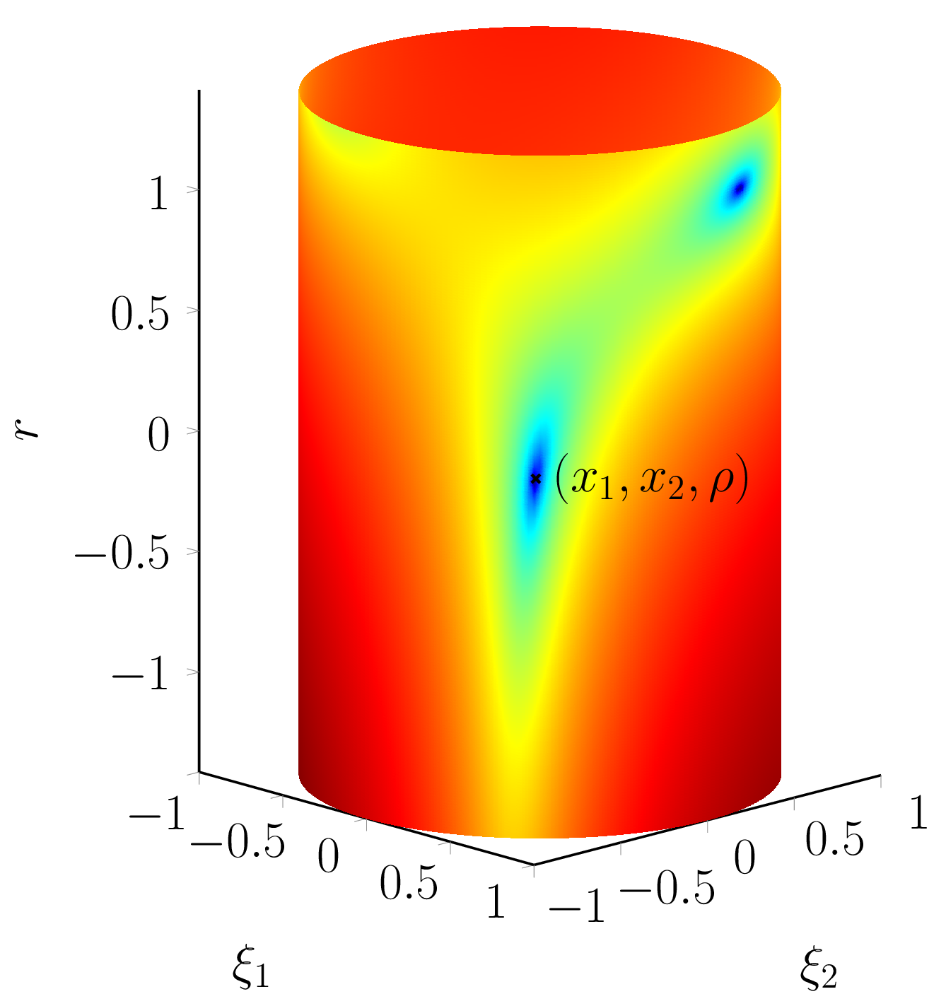
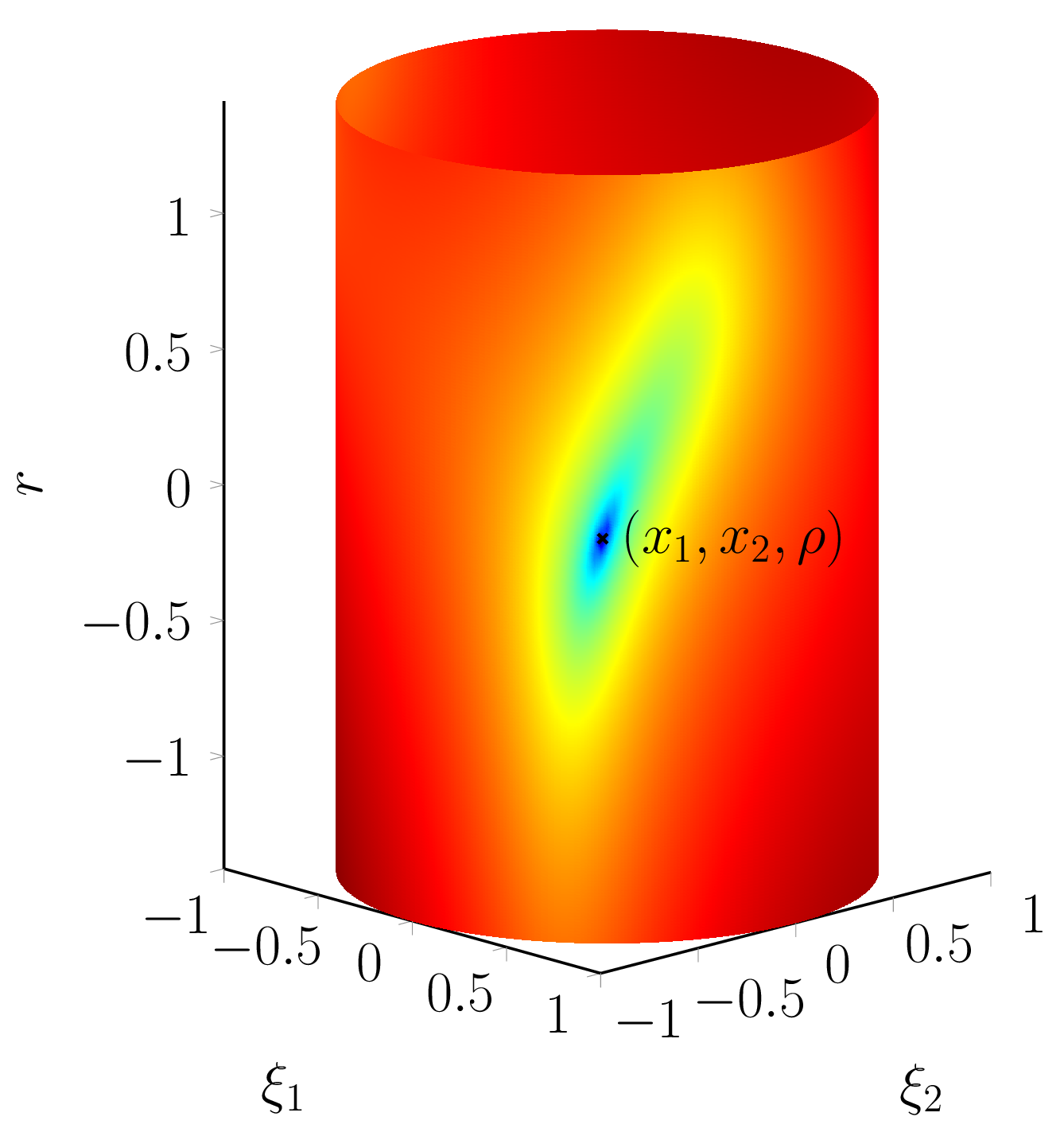
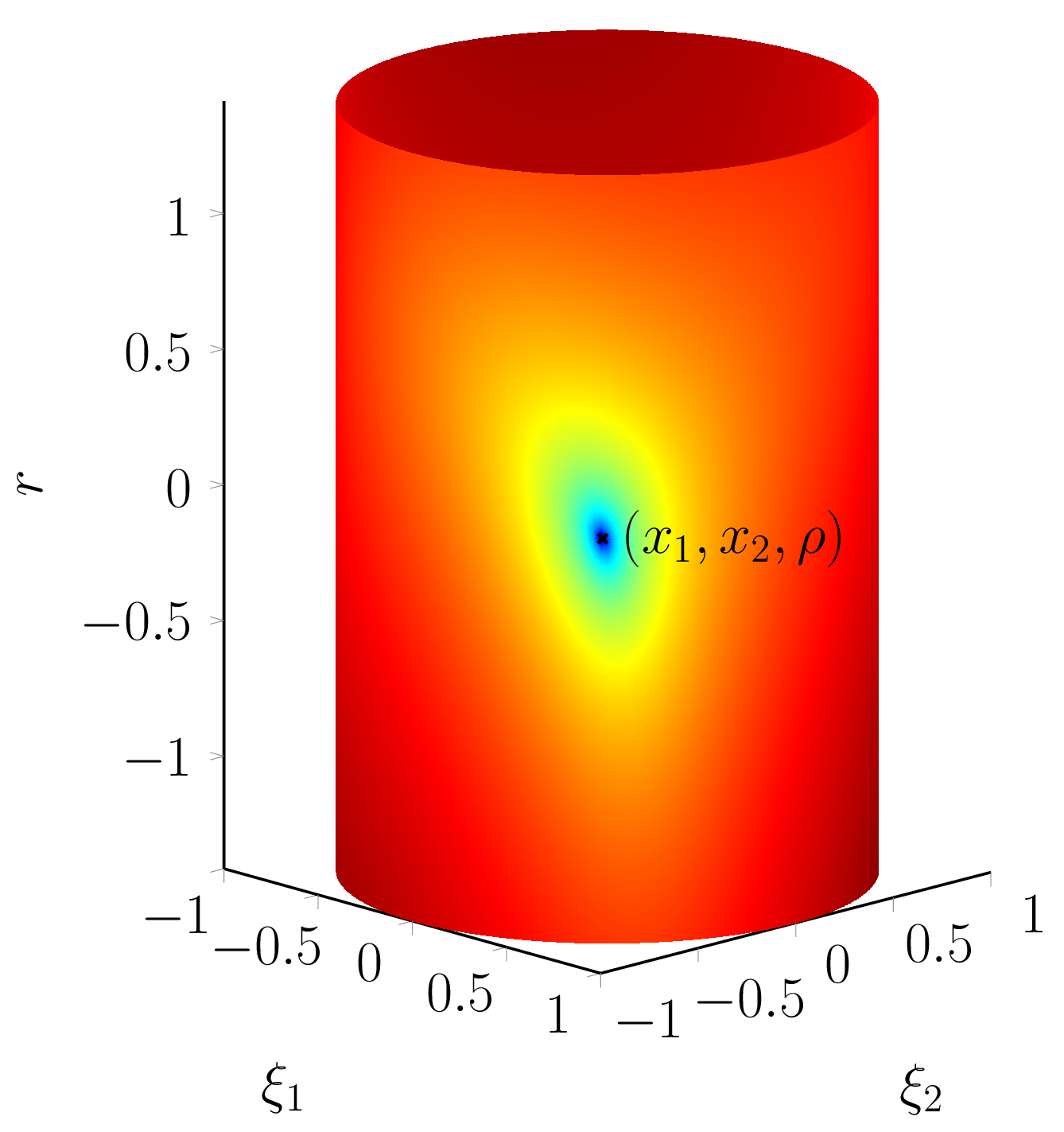
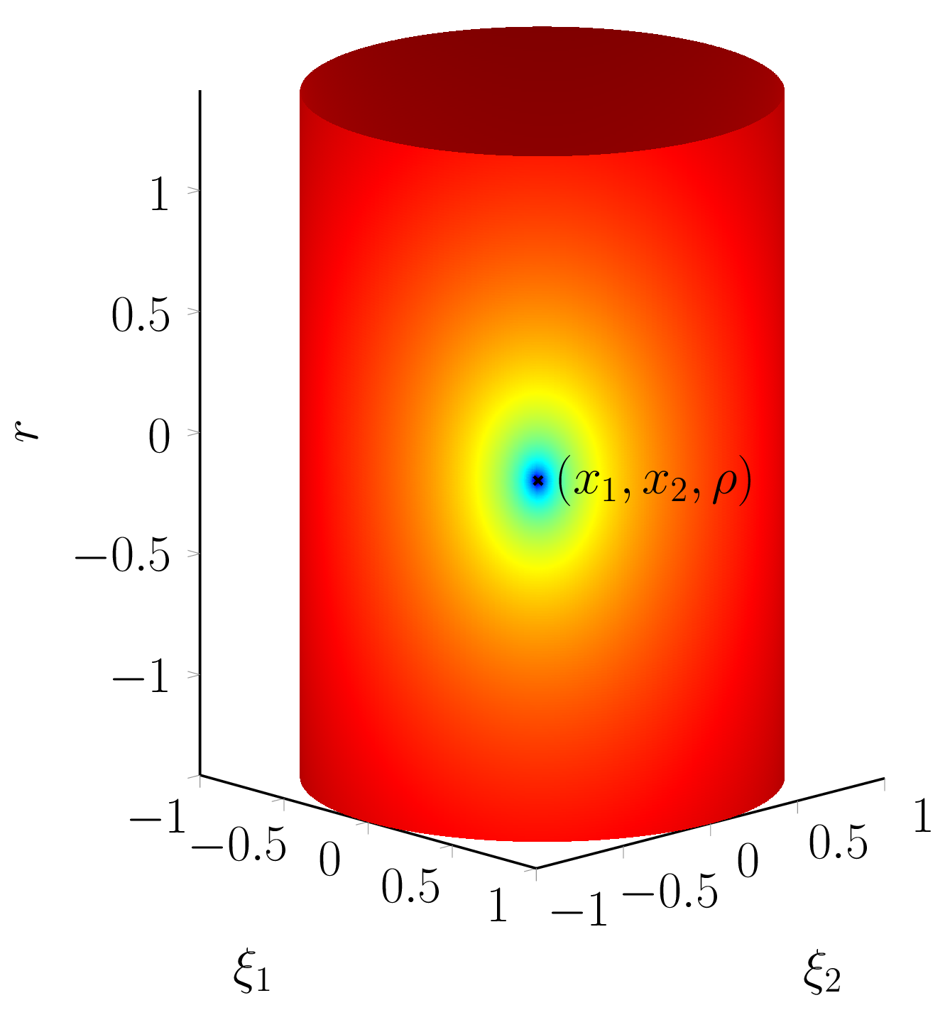
To do this, we look at the geometric behaviour of the objective minimised in (2.2) to understand whether a region exists where the problem shows local convexity. Intuitively, we generate a random instance of (1.1) for n=2𝑛2n=2, m=2𝑚2m=2 and 𝒂i,li.i.d.𝒩(𝟎n,𝑰n)subscriptsimilar-toi.i.d.subscript𝒂𝑖𝑙𝒩subscript0𝑛subscript𝑰𝑛\boldsymbol{a}_{i,l}\sim_{\rm\textrm{i.i.d.}}\mathcal{N}(\boldsymbol{0}_{n},\boldsymbol{I}_{n}), with (𝒙,𝒈)(12[11],𝟏2+225[11])=(𝒙,𝒈)𝒙𝒈12superscriptdelimited-[]11topsubscript12225superscriptdelimited-[]11top𝒙𝒈({\boldsymbol{x}},\boldsymbol{g})\coloneqq\big{(}\tfrac{1}{\sqrt{2}}[1-1]^{\top},\boldsymbol{1}_{2}+\tfrac{\sqrt{2}}{25}[1-1]^{\top}\big{)}=({\boldsymbol{x}},\boldsymbol{g}). The amount of snapshots is varied as p={20,21,,}𝑝superscript20superscript21p=\{2^{0},2^{1},\,\cdots,\infty\}. We measure the logf(𝝃,𝜸)𝑓𝝃𝜸\log f({\boldsymbol{\xi}},{\boldsymbol{\gamma}}) for 𝝃𝕊21𝝃subscriptsuperscript𝕊12{\boldsymbol{\xi}}\in\mathbb{S}^{1}_{2} and 𝜸=𝟏2+r12[11]𝒢ρ𝜸subscript12𝑟12superscriptdelimited-[]11topsubscript𝒢𝜌{\boldsymbol{\gamma}}=\boldsymbol{1}_{2}+r\tfrac{1}{\sqrt{2}}[\begin{smallmatrix}1&-1\end{smallmatrix}]^{\top}\in{\mathcal{G}}_{\rho} depending only on a parameter r<ρ𝑟𝜌r<\rho. As for the case p𝑝p\rightarrow\infty we simply report the logarithm of 𝔼f(𝝃,𝜸)𝔼𝑓𝝃𝜸\operatorname{{\mathbb{E}}}f({\boldsymbol{\xi}},{\boldsymbol{\gamma}}) in Fig. 1. As mp>n+m𝑚𝑝𝑛𝑚mp>n+m there is one global minimiser at (𝒙,𝒈)𝒙𝒈({\boldsymbol{x}},{\boldsymbol{g}}) for r=ρ=8102𝑟𝜌8superscript102r=\rho=8\cdot 10^{-2}, whose neighbourhood exhibits a smooth behaviour suggesting local convexity as p𝑝p increases, and thus the existence of a basin of attraction around the minimiser. In other words, there will be a critical value of mp𝑚𝑝mp for which the objective function behaves arbitrarily close to its expectation which, as we will see below and suggested by our example, is indeed locally convex for sufficiently small values of κ,ρ𝜅𝜌\kappa,\rho. This property is investigated in the following section.
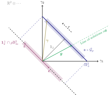
Refer to caption (a) Summary of geometric considerations in the gain domain Refer to caption (b) p=1𝑝1p=1 Refer to caption (c) p=2𝑝2p=2 Refer to caption (d) p=4𝑝4p=4 Refer to caption (e) Expectation (p)𝑝(p\rightarrow\infty)

Figure 1: Geometric intuition on an instance of (2.2) for n=2,m=2formulae-sequence𝑛2𝑚2n=2,m=2: graphical representation of the parametrisation of the gain domain (a); heat map of logf(𝝃,𝜸)𝑓𝝃𝜸\log f({\boldsymbol{\xi}},{\boldsymbol{\gamma}}) for the numerical example given in the text at 𝝃=1norm𝝃1\|{\boldsymbol{\xi}}\|=1 and increasing p𝑝p\rightarrow\infty (b–e). The vertical axis reports the parameter r[2,2]𝑟22r\in[-\sqrt{2},\sqrt{2}].

2.2.3 Local Convexity in Expectation

We proceed by highlighting two basic facts regarding (2.2) for p𝑝p\rightarrow\infty, a case that is reported in Table 1, where all finite-sample expressions of the quantities therein are unbiased estimates of their expectation with respect to the i.i.d. sensing vectors 𝒂i,lsubscript𝒂𝑖𝑙\boldsymbol{a}_{i,l}. To begin with, we define a set of test vectors 𝒱n×𝟏m𝒱superscript𝑛subscriptsuperscript1perpendicular-to𝑚\mathcal{V}\coloneqq\mathbb{R}^{n}\times{{\boldsymbol{1}}^{\perp}_{m}} used in the two following results. This is simply the set of all test vectors in the product space that are orthogonal to the direction 𝟏msubscript1𝑚\boldsymbol{1}_{m} in the gain domain. The proof of all following statements in this section is reported in App. B.

Proposition 2.1 (Global minimiser in expectation of (2.2)).

In expectation, the only stationary point of (2.2) is (𝐱,𝐠)(𝐠1m𝐱,m𝐠1𝐠)𝐱𝐠subscriptnorm𝐠1𝑚𝐱𝑚subscriptnorm𝐠1𝐠\textstyle({\boldsymbol{x}},{\boldsymbol{g}})\coloneqq\big{(}\tfrac{\|{\boldsymbol{g}}\|_{1}}{m}{\boldsymbol{x}},\tfrac{m}{\|{\boldsymbol{g}}\|_{1}}{\boldsymbol{g}}\big{)}. There, we have that 𝔼f(𝐱,𝐠)𝒱0subscriptsucceeds𝒱𝔼superscriptperpendicular-to𝑓𝐱𝐠0\operatorname{{\mathbb{E}}}\mathcal{H}^{\perp}f({\boldsymbol{x}},{\boldsymbol{g}})\succ_{\mathcal{V}}0.

Once this stationary point is established, simple analysis of the projected Hessian matrix in expectation for all (𝝃,𝜸)𝒟κ,ρ𝝃𝜸subscript𝒟𝜅𝜌({\boldsymbol{\xi}},{\boldsymbol{\gamma}})\in{{\mathcal{D}}}_{\kappa,\rho} shows the following Proposition.

Proposition 2.2 (Convexity in expectation of (2.2) in a (κ,ρ)𝜅𝜌(\kappa,\rho)-neighbourhood).

For any (𝛏,𝛄)𝒟κ,ρ𝛏𝛄subscript𝒟𝜅𝜌({\boldsymbol{\xi}},{\boldsymbol{\gamma}})\in{\mathcal{D}}_{\kappa,\rho} for some κ[0,1),ρ[0,13κm(1κ))formulae-sequence𝜅01𝜌013𝜅𝑚1𝜅\textstyle{\kappa\in[0,1),\rho\in\left[0,1-\tfrac{\sqrt{3}\kappa}{\sqrt{m}(1-\kappa)}\right)}, we have that 𝔼f(𝛏,𝛄)𝒱0subscriptsucceeds𝒱𝔼superscriptperpendicular-to𝑓𝛏𝛄0\operatorname{{\mathbb{E}}}\mathcal{H}^{\perp}f({\boldsymbol{\xi}},{\boldsymbol{\gamma}})\succ_{\mathcal{V}}0.

We remark two interesting aspects of the upper bound ρ<13κm(1κ)𝜌13𝜅𝑚1𝜅\rho<1-\tfrac{\sqrt{3}\kappa}{\sqrt{m}(1-\kappa)}. Note how this can be made arbitrarily close to 111 both when m𝑚m\rightarrow\infty, i.e., asymptotically in the number of measurements, and when κ0𝜅0\kappa\rightarrow 0, i.e., when the basin of attraction is made arbitrarily small around the global minimiser.

Thus, in expectation (2.2) is locally convex on 𝒟κ,ρsubscript𝒟𝜅𝜌{{\mathcal{D}}}_{\kappa,\rho} when the variations with respect to the gain domain are taken on 𝟏msubscriptsuperscript1perpendicular-to𝑚{{\boldsymbol{1}}^{\perp}_{m}}. However, this last information is not particularly useful in practice, since in expectation we would already have an unbiased estimate of 𝒙𝒙{\boldsymbol{x}} in the form of 𝝃0subscript𝝃0{\boldsymbol{\xi}}_{0} in Table 1, from which 𝒈𝒈{\boldsymbol{g}} would be easily obtained. This would suggest the need for a non-asymptotic analysis to check the requirements on mp𝑚𝑝mp needed to benefit of the consequences of local convexity for finite p𝑝p. Rather than testing local convexity by the positive-semidefiniteness of the Hessian matrix (as done, e.g., in Sanghavi et al. [12]) the theory we develop in Sec. 3.2 follows the methodology of Candès et al. [11], i.e., a simple first-order analysis of the local properties of the gradient f(𝝃,𝜸)superscriptbold-∇perpendicular-to𝑓𝝃𝜸\boldsymbol{\nabla}^{\perp}f({\boldsymbol{\xi}},{\boldsymbol{\gamma}}) and initialisation point (𝝃0,𝜸0)subscript𝝃0subscript𝜸0({\boldsymbol{\xi}}_{0},{\boldsymbol{\gamma}}_{0}) which suffice to prove our recovery guarantees.

3 Blind Calibration by Projected Gradient Descent

In this section we discuss the actual algorithm used to solve (2.2) in its non-convex form with the observations made in Sec. 2. The algorithm is a simple projected gradient descent, as detailed below. We proceed by stating our method and providing right after the recovery guarantees ensured by a sample complexity requirement given on mp𝑚𝑝mp.

3.1 Descent Algorithm

The solution of (2.2) is here obtained as summarised in Alg. 1 and consists of an initialisation (𝝃0,𝜸0)subscript𝝃0subscript𝜸0({\boldsymbol{\xi}}_{0},{\boldsymbol{\gamma}}_{0}) followed by projected gradient descent. Similarly to [11] we have chosen an initialisation 𝝃0subscript𝝃0{\boldsymbol{\xi}}_{0} that is an unbiased estimator of the exact signal-domain solution as p𝑝p\rightarrow\infty, i.e.𝔼𝝃0=𝒙𝔼subscript𝝃0𝒙\operatorname{{\mathbb{E}}}{\boldsymbol{\xi}}_{0}={\boldsymbol{x}}. This is indicated in Table 1 and straightforward since 𝔼𝒂i,l𝒂i,l=𝑰n𝔼subscript𝒂𝑖𝑙superscriptsubscript𝒂𝑖𝑙topsubscript𝑰𝑛\operatorname{{\mathbb{E}}}\boldsymbol{a}_{i,l}\boldsymbol{a}_{i,l}^{\top}=\boldsymbol{I}_{n}. For p<𝑝p<\infty we will show in Prop. 3.1 that, for mp(n+m)logngreater-than-or-equivalent-to𝑚𝑝𝑛𝑚𝑛mp\gtrsim(n+m)\log n and sufficiently large n𝑛n, the initialisation lands in (𝝃0,𝜸0)𝒟κ,ρsubscript𝝃0subscript𝜸0subscript𝒟𝜅𝜌({\boldsymbol{\xi}}_{0},{\boldsymbol{\gamma}}_{0})\in{\mathcal{D}}_{{\kappa},\rho} for ρ[0,1)𝜌01\rho\in[0,1) and κ>0𝜅0\kappa>0 with high probability. As for the gains, we initialise 𝜸0𝟏m(𝜺0𝟎m)subscript𝜸0subscript1𝑚subscript𝜺0subscript0𝑚{\boldsymbol{\gamma}}_{0}\coloneqq\boldsymbol{1}_{m}\ (\boldsymbol{\varepsilon}_{0}\coloneqq\boldsymbol{0}_{m}). This initialisation allows us to establish the radius of the basin of attraction around (𝒙,𝒈)𝒙𝒈({\boldsymbol{x}},{\boldsymbol{g}}). As a minor advantage, let us also remark that this initialisation is specific to our sensing model, but computationally cheaper than spectral initialisations such as those proposed in [11, 20].

Since ρ<1𝜌1\rho<1 is small, we perform a few simplifications to devise our solver to (2.2). While generally we would need to project555Computationally this projection is entirely feasible, but would critically complicate the proofs. any step in 𝜸𝜸{\boldsymbol{\gamma}} on 𝒢ρsubscript𝒢𝜌\mathcal{G}_{\rho}, we first update the gains with the projected gradient 𝜸f(𝝃j,𝜸j)subscriptsuperscriptbold-∇perpendicular-to𝜸𝑓subscript𝝃𝑗subscript𝜸𝑗\boldsymbol{\nabla}^{\perp}_{\boldsymbol{\gamma}}f({\boldsymbol{\xi}}_{j},{\boldsymbol{\gamma}}_{j}) in step 5 (see Table 1 for its expression). Then we apply 𝒫𝒢ρsubscript𝒫subscript𝒢𝜌{\mathcal{P}}_{{\mathcal{G}}_{\rho}}, i.e., the projector on the closed convex set 𝒢ρsubscript𝒢𝜌{{\mathcal{G}}_{\rho}} (step 6). This is algorithmically easy, as it can be obtained by, e.g., alternate projection on convex sets666Indeed, 𝒫𝒢ρsubscript𝒫subscript𝒢𝜌{\mathcal{P}}_{{\mathcal{G}}_{\rho}} is obtained algorithmically by simple alternate projections between 𝑷𝟏msubscript𝑷subscriptsuperscript1perpendicular-to𝑚{\boldsymbol{P}}_{{{\boldsymbol{1}}^{\perp}_{m}}} and 𝒫ρ𝔹msubscript𝒫𝜌subscriptsuperscript𝔹𝑚{\mathcal{P}}_{\rho\,{\mathbb{B}}^{m}_{\infty}} and adding 𝟏msubscript1𝑚\boldsymbol{1}_{m} to the output.. However, this step is merely a formal requirement to ensure that each iterate 𝜸j+1𝒢ρΠ+msubscript𝜸𝑗1subscript𝒢𝜌subscriptsuperscriptΠ𝑚{\boldsymbol{\gamma}}_{j+1}\in{\mathcal{G}}_{\rho}\subset\Pi^{m}_{+} for some fixed ρ𝜌\rho when proving the convergence of Alg. 1 to (𝒙,𝒈)𝒙𝒈({\boldsymbol{x}},{\boldsymbol{g}}), but practically not needed, as we have observed that step 6 can be omitted since 𝜸ˇj+1𝒢ρsubscriptˇ𝜸𝑗1subscript𝒢𝜌\check{{\boldsymbol{\gamma}}}_{j+1}\in{\mathcal{G}}_{\rho} is always verified in our experiments.

Thus, Alg. 1 is as simple and efficient as a first-order descent algorithm with the projected gradient f(𝝃,𝜸)superscriptbold-∇perpendicular-to𝑓𝝃𝜸\boldsymbol{\nabla}^{\perp}f({\boldsymbol{\xi}},{\boldsymbol{\gamma}}). The proposed version performs two line searches in step 3 that can be solved in closed-form at each iteration, as made clearer in Sec. 6.1. These searches are simply introduced to improve the convergence rate, but are not necessary and could be replaced by a careful choice of some fixed steps μ𝝃,μ𝜸>0subscript𝜇𝝃subscript𝜇𝜸0\mu_{\boldsymbol{\xi}},\mu_{\boldsymbol{\gamma}}>0 (for which, in fact, our main theoretical results are developed).

Algorithm 1 Non-Convex Blind Calibration by Projected Gradient Descent.
1:  Initialise 𝝃01mpl=1p(𝑨l)𝒚l,𝜸0𝟏m,j0formulae-sequencesubscript𝝃01𝑚𝑝subscriptsuperscript𝑝𝑙1superscriptsubscript𝑨𝑙topsubscript𝒚𝑙formulae-sequencesubscript𝜸0subscript1𝑚𝑗0{\boldsymbol{\xi}}_{0}\coloneqq\tfrac{1}{mp}\sum^{p}_{l=1}\left({\boldsymbol{A}}_{l}\right)^{\top}{\boldsymbol{y}}_{l},\,{\boldsymbol{\gamma}}_{0}\coloneqq\boldsymbol{1}_{m},\,j\coloneqq 0.
2:  while stop criteria not met do
3:     {μ𝝃argminυf(𝝃jυ𝝃f(𝝃j,𝜸j),𝜸j)μ𝜸argminυf(𝝃j,𝜸jυ𝜸f(𝝃j,𝜸j))casessubscript𝜇𝝃subscriptargmin𝜐𝑓subscript𝝃𝑗𝜐subscriptbold-∇𝝃𝑓subscript𝝃𝑗subscript𝜸𝑗subscript𝜸𝑗otherwisesubscript𝜇𝜸subscriptargmin𝜐𝑓subscript𝝃𝑗subscript𝜸𝑗𝜐subscriptsuperscriptbold-∇perpendicular-to𝜸𝑓subscript𝝃𝑗subscript𝜸𝑗otherwise\begin{cases}\mu_{\boldsymbol{\xi}}\coloneqq\operatorname{{argmin}}_{\upsilon\in\mathbb{R}}f({\boldsymbol{\xi}}_{j}-\upsilon\boldsymbol{\nabla}_{\boldsymbol{\xi}}f({{\boldsymbol{\xi}}_{j},{\boldsymbol{\gamma}}_{j}}),{\boldsymbol{\gamma}}_{j})\\ \mu_{\boldsymbol{\gamma}}\coloneqq\operatorname{{argmin}}_{\upsilon\in\mathbb{R}}f({\boldsymbol{\xi}}_{j},{\boldsymbol{\gamma}}_{j}-\upsilon\boldsymbol{\nabla}^{\perp}_{\boldsymbol{\gamma}}f({{\boldsymbol{\xi}}_{j},{\boldsymbol{\gamma}}_{j}}))\end{cases}
4:     𝝃j+1𝝃jμ𝝃𝝃f(𝝃j,𝜸j)subscript𝝃𝑗1subscript𝝃𝑗subscript𝜇𝝃subscriptbold-∇𝝃𝑓subscript𝝃𝑗subscript𝜸𝑗{\boldsymbol{\xi}}_{j+1}\coloneqq{\boldsymbol{\xi}}_{j}-\mu_{\boldsymbol{\xi}}\boldsymbol{\nabla}_{\boldsymbol{\xi}}f({{\boldsymbol{\xi}}_{j},{\boldsymbol{\gamma}}_{j}})
5:     𝜸ˇj+1𝜸jμ𝜸𝜸f(𝝃j,𝜸j)subscriptˇ𝜸𝑗1subscript𝜸𝑗subscript𝜇𝜸subscriptsuperscriptbold-∇perpendicular-to𝜸𝑓subscript𝝃𝑗subscript𝜸𝑗\check{{\boldsymbol{\gamma}}}_{j+1}\coloneqq{\boldsymbol{\gamma}}_{j}-\mu_{\boldsymbol{\gamma}}\,\boldsymbol{\nabla}^{\perp}_{\boldsymbol{\gamma}}f({{\boldsymbol{\xi}}_{j},{\boldsymbol{\gamma}}_{j}})
6:     𝜸j+1𝒫𝒢ρ𝜸ˇj+1subscript𝜸𝑗1subscript𝒫subscript𝒢𝜌subscriptˇ𝜸𝑗1{{\boldsymbol{\gamma}}}_{j+1}\coloneqq{\mathcal{P}}_{{\mathcal{G}}_{\rho}}\check{{\boldsymbol{\gamma}}}_{j+1}
7:     jj+1𝑗𝑗1j\coloneqq j+1
8:  end while

3.2 Convergence Guarantees

We now obtain the conditions that ensure convergence of this descent algorithm to the exact solution (𝒙,𝒈)𝒙𝒈({\boldsymbol{x}},{\boldsymbol{g}}) for some fixed step sizes μ𝝃,μ𝜸subscript𝜇𝝃subscript𝜇𝜸\mu_{\boldsymbol{\xi}},\mu_{\boldsymbol{\gamma}}. This is done in three steps: (i)𝑖(i) the initialisation (𝝃0,𝜸0)subscript𝝃0subscript𝜸0({\boldsymbol{\xi}}_{0},{\boldsymbol{\gamma}}_{0}) is shown to lie in 𝒟κ,ρsubscript𝒟𝜅𝜌{\mathcal{D}}_{{\kappa},\rho} for ρ[0,1)𝜌01\rho\in[0,1) and some small κ𝜅\kappa with high probability, i.e., the probability that this is not verified decays exponentially in the problem dimensions; (ii)𝑖𝑖(ii) uniformly on 𝒟κ,ρsubscript𝒟𝜅𝜌{\mathcal{D}}_{{\kappa},\rho} we are able to show that, with high probability, a gradient descent update decreases the distance to (𝒙,𝒈)𝒙𝒈({\boldsymbol{x}},{\boldsymbol{g}}) by bounding the magnitude of f(𝝃,𝜸)superscriptbold-∇perpendicular-to𝑓𝝃𝜸\boldsymbol{\nabla}^{\perp}f({\boldsymbol{\xi}},{\boldsymbol{\gamma}}) as well as its angle with the direction of the global minimiser; (iii)𝑖𝑖𝑖(iii) still by uniformity, applying this property to any iterate (𝝃j,𝜸j)subscript𝝃𝑗subscript𝜸𝑗({\boldsymbol{\xi}}_{j},{\boldsymbol{\gamma}}_{j}) of Alg. 1 leads to finding some fixed step values μ𝝃,μ𝜸subscript𝜇𝝃subscript𝜇𝜸\mu_{\boldsymbol{\xi}},\mu_{\boldsymbol{\gamma}} that grant convergence to (𝒙,𝒈)𝒙𝒈({\boldsymbol{x}},{\boldsymbol{g}}) as j𝑗j\rightarrow\infty, i.e., what is commonly referred to as linear convergence (with respect to logj𝑗\log j). The proofs of all following statements in this section are reported in App. C. The general proof strategy relies on concentration inequalities for functions of our i.i.d. sub-Gaussian sensing vectors 𝒂i,lsubscript𝒂𝑖𝑙{\boldsymbol{a}_{i,l}} as well as a particular application of matrix Bernstein’s inequality. These fundamental mathematical tools are defined in App. A.

We first focus on the initialisation and assess its non-asymptotic properties in terms of the distance attained with respect to the global minimiser.

Proposition 3.1 (Initialisation Proximity).

Let (𝛏0,𝛄0)subscript𝛏0subscript𝛄0({\boldsymbol{\xi}}_{0},{\boldsymbol{\gamma}}_{0}) be as in Table 1. Given δ(0,1)𝛿01{\delta}\in(0,1), t1𝑡1t\geq 1, provided mpδ2(n+m)lognδgreater-than-or-equivalent-to𝑚𝑝superscript𝛿2𝑛𝑚𝑛𝛿\textstyle mp\gtrsim{\delta}^{-2}(n+m)\log\tfrac{n}{\delta} and ntlogmpgreater-than-or-equivalent-to𝑛𝑡𝑚𝑝n\gtrsim t\log mp, with probability exceeding

1Cecδ2mp(mp)t1𝐶superscript𝑒𝑐superscript𝛿2𝑚𝑝superscript𝑚𝑝𝑡1-Ce^{-c{\delta}^{2}mp}-(mp)^{-t} (3.1)

for some C,c>0𝐶𝑐0C,c>0, we have that 𝛏0𝐱δ𝐱normsubscript𝛏0𝐱𝛿norm𝐱\|{\boldsymbol{\xi}}_{0}-{\boldsymbol{x}}\|\leq{\delta}\|{\boldsymbol{x}}\|. Since 𝛄0𝟏msubscript𝛄0subscript1𝑚{\boldsymbol{\gamma}}_{0}\coloneqq\boldsymbol{1}_{m} we also have 𝛄0𝐠ρ<1subscriptnormsubscript𝛄0𝐠𝜌1\|{\boldsymbol{\gamma}}_{0}-{\boldsymbol{g}}\|_{\infty}\leq\rho<1. Thus (𝛏0,𝛄0)𝒟κ,ρsubscript𝛏0subscript𝛄0subscript𝒟𝜅𝜌({\boldsymbol{\xi}}_{0},{\boldsymbol{\gamma}}_{0})\in{\mathcal{D}}_{{\kappa},\rho} with the same probability and κ0δ2+ρ2subscript𝜅0superscript𝛿2superscript𝜌2\kappa_{0}\coloneqq\sqrt{\delta^{2}+\rho^{2}}.

Secondly, we develop the requirements for convergence, i.e., for 𝒟κ0,ρsubscript𝒟subscript𝜅0𝜌{\mathcal{D}}_{{\kappa_{0}},\rho} to be a basin of attraction around the global minimiser. Provided that the initialisation lands in 𝒟κ0,ρsubscript𝒟subscript𝜅0𝜌{\mathcal{D}}_{{\kappa_{0}},\rho}, any update from (𝝃,𝜸)𝒟κ0,ρ𝝃𝜸subscript𝒟subscript𝜅0𝜌({\boldsymbol{\xi}},{\boldsymbol{\gamma}})\in{\mathcal{D}}_{{\kappa_{0}},\rho} to some 𝝃+𝝃μ𝝃𝝃f(𝝃,𝜸),𝜸ˇ+𝜸μ𝜸𝜸f(𝝃,𝜸)formulae-sequencesubscript𝝃𝝃subscript𝜇𝝃subscriptbold-∇𝝃𝑓𝝃𝜸subscriptˇ𝜸𝜸subscript𝜇𝜸subscriptsuperscriptbold-∇perpendicular-to𝜸𝑓𝝃𝜸{\boldsymbol{\xi}}_{+}\coloneqq{\boldsymbol{\xi}}-\mu_{\boldsymbol{\xi}}\boldsymbol{\nabla}_{\boldsymbol{\xi}}f({{\boldsymbol{\xi}},{\boldsymbol{\gamma}}}),\check{{\boldsymbol{\gamma}}}_{+}\coloneqq{\boldsymbol{\gamma}}-\mu_{\boldsymbol{\gamma}}\boldsymbol{\nabla}^{\perp}_{\boldsymbol{\gamma}}f({{\boldsymbol{\xi}},{\boldsymbol{\gamma}}}) has distance from the solution

Δ(𝝃+,𝜸ˇ+)Δsubscript𝝃subscriptˇ𝜸\displaystyle{\Delta}({\boldsymbol{\xi}}_{+},\check{{\boldsymbol{\gamma}}}_{+}) =Δ(𝝃,𝜸)2(μ𝝃𝝃f(𝝃,𝜸),𝝃𝒙+μ𝜸𝒙2m𝜸f(𝝃,𝜸),𝜸𝒈)absentΔ𝝃𝜸2subscript𝜇𝝃subscriptbold-∇𝝃𝑓𝝃𝜸𝝃𝒙subscript𝜇𝜸superscriptnorm𝒙2𝑚subscriptsuperscriptbold-∇perpendicular-to𝜸𝑓𝝃𝜸𝜸𝒈\displaystyle={\Delta}({\boldsymbol{\xi}},{\boldsymbol{\gamma}})-2\big{(}\mu_{\boldsymbol{\xi}}\langle\boldsymbol{\nabla}_{\boldsymbol{\xi}}f({\boldsymbol{\xi}},{\boldsymbol{\gamma}}),{\boldsymbol{\xi}}-{\boldsymbol{x}}\rangle+\mu_{\boldsymbol{\gamma}}\tfrac{\|{\boldsymbol{x}}\|^{2}}{m}\langle\boldsymbol{\nabla}^{\perp}_{\boldsymbol{\gamma}}f({\boldsymbol{\xi}},{\boldsymbol{\gamma}}),{\boldsymbol{\gamma}}-{\boldsymbol{g}}\rangle\big{)}
+μ𝝃2𝝃f(𝝃,𝜸)2+μ𝜸2𝒙2m𝜸f(𝝃,𝜸)2.superscriptsubscript𝜇𝝃2superscriptnormsubscriptbold-∇𝝃𝑓𝝃𝜸2superscriptsubscript𝜇𝜸2superscriptnorm𝒙2𝑚superscriptnormsubscriptsuperscriptbold-∇perpendicular-to𝜸𝑓𝝃𝜸2\displaystyle\quad+{\mu_{\boldsymbol{\xi}}^{2}}\|\boldsymbol{\nabla}_{\boldsymbol{\xi}}f({\boldsymbol{\xi}},{\boldsymbol{\gamma}})\|^{2}+{\mu_{\boldsymbol{\gamma}}^{2}}\tfrac{\|{\boldsymbol{x}}\|^{2}}{m}\|\boldsymbol{\nabla}^{\perp}_{\boldsymbol{\gamma}}f({\boldsymbol{\xi}},{\boldsymbol{\gamma}})\|^{2}. (3.2)

As detailed in App. C, it is therefore clear from (3.2) that a lower bound on f(𝝃,𝜸),[(𝝃𝒙)(𝜸𝒈)]superscriptbold-∇perpendicular-to𝑓𝝃𝜸superscriptdelimited-[]superscript𝝃𝒙topsuperscript𝜸𝒈toptop\big{\langle}\boldsymbol{\nabla}^{\perp}f({\boldsymbol{\xi}},{\boldsymbol{\gamma}}),\,[({\boldsymbol{\xi}}-{\boldsymbol{x}})^{\top}({\boldsymbol{\gamma}}-{\boldsymbol{g}})^{\top}]^{\top}\big{\rangle} and upper bounds on both 𝝃f(𝝃,𝜸)normsubscriptbold-∇𝝃𝑓𝝃𝜸\|\boldsymbol{\nabla}_{\boldsymbol{\xi}}f({\boldsymbol{\xi}},{\boldsymbol{\gamma}})\| and 𝜸f(𝝃,𝜸)normsubscriptsuperscriptbold-∇perpendicular-to𝜸𝑓𝝃𝜸\|\boldsymbol{\nabla}^{\perp}_{\boldsymbol{\gamma}}f({\boldsymbol{\xi}},{\boldsymbol{\gamma}})\|, holding for all points in 𝒟κ0,ρsubscript𝒟subscript𝜅0𝜌{\mathcal{D}}_{{\kappa_{0}},\rho} will yield the requirements to attain the desired convergent behaviour (for sufficiently small step sizes), also provided these bounds can be expressed as a function of Δ(𝝃,𝜸)Δ𝝃𝜸\Delta({\boldsymbol{\xi}},{\boldsymbol{\gamma}}). This leads to the following proposition formulated for a general neighbourhood of radius κ>0𝜅0\kappa>0.

Proposition 3.2 (Regularity condition in 𝒟κ,ρsubscript𝒟𝜅𝜌{\mathcal{D}}_{{\kappa},\rho}).

Given δ(0,1)𝛿01\delta\in(0,1), t1𝑡1t\geq 1 and κ>0𝜅0\kappa>0, provided ρ<14δ31𝜌14𝛿31\rho<\tfrac{1-4\delta}{31} and

n𝑛\displaystyle\textstyle n tlog(mp),greater-than-or-equivalent-toabsent𝑡𝑚𝑝\displaystyle\textstyle\gtrsim t\log(mp),
mp𝑚𝑝\displaystyle\textstyle mp tδ2(n+m)log2(m(p+n))log(1δ).greater-than-or-equivalent-toabsent𝑡superscript𝛿2𝑛𝑚superscript2𝑚𝑝𝑛1𝛿\displaystyle\textstyle\gtrsim t\delta^{-2}(n+m)\,\log^{2}(m(p+n))\log(\frac{1}{\delta}).

with probability exceeding 1C(mp)t1𝐶superscript𝑚𝑝𝑡1-C(mp)^{-t} for some C>0𝐶0C>0, we have for all (𝛏,𝛄)𝒟κ,ρ𝛏𝛄subscript𝒟𝜅𝜌({\boldsymbol{\xi}},{\boldsymbol{\gamma}})\in{\mathcal{D}}_{{\kappa},\rho}

f(𝝃,𝜸),[𝝃𝒙𝜸𝒈]superscriptbold-∇perpendicular-to𝑓𝝃𝜸matrix𝝃𝒙𝜸𝒈\displaystyle\left\langle\boldsymbol{\nabla}^{\perp}f({\boldsymbol{\xi}},{\boldsymbol{\gamma}}),\begin{bmatrix}{\boldsymbol{\xi}}-{\boldsymbol{x}}\\ {\boldsymbol{\gamma}}-{\boldsymbol{g}}\end{bmatrix}\right\rangle ηΔ(𝝃,𝜸),absent𝜂Δ𝝃𝜸\displaystyle\geq\eta\,{\Delta}({\boldsymbol{\xi}},{\boldsymbol{\gamma}}), (3.3)
𝝃f(𝝃,𝜸)2superscriptnormsubscriptbold-∇𝝃𝑓𝝃𝜸2\displaystyle\|\boldsymbol{\nabla}_{\boldsymbol{\xi}}f({\boldsymbol{\xi}},{\boldsymbol{\gamma}})\|^{2} L𝝃2Δ(𝝃,𝜸),absentsuperscriptsubscript𝐿𝝃2Δ𝝃𝜸\displaystyle\leq L_{\boldsymbol{\xi}}^{2}\ {\Delta}({\boldsymbol{\xi}},{\boldsymbol{\gamma}}), (3.4)
𝜸f(𝝃,𝜸)2superscriptnormsuperscriptsubscriptbold-∇𝜸perpendicular-to𝑓𝝃𝜸2\displaystyle\|\boldsymbol{\nabla}_{\boldsymbol{\gamma}}^{\perp}f({\boldsymbol{\xi}},{\boldsymbol{\gamma}})\|^{2} L𝜸2Δ(𝝃,𝜸),absentsuperscriptsubscript𝐿𝜸2Δ𝝃𝜸\displaystyle\leq L_{\boldsymbol{\gamma}}^{2}\ {\Delta}({\boldsymbol{\xi}},{\boldsymbol{\gamma}}), (3.5)

where η131ρ4δ(0,1)𝜂131𝜌4𝛿01\eta\coloneqq 1-31\rho-4\delta\in(0,1), L𝛏=82subscript𝐿𝛏82L_{\boldsymbol{\xi}}=8\sqrt{2} and L𝛄42(1+κ)𝐱subscript𝐿𝛄421𝜅norm𝐱L_{\boldsymbol{\gamma}}\coloneqq 4\sqrt{2}(1+\kappa)\|\boldsymbol{x}\|.

The interpretation of (3.3), (3.4) and (3.5) is clear, and analogue to the method pursued by Candès et al. [11] in the context of phase retrieval. The first condition or bounded curvature ensures that the angle between the gradient and the direction of the global minimiser is not too large. The second condition or Lipschitz gradient gives a bound on the maximum magnitude that the gradient is allowed to assume. Moreover, the bounded curvature in (3.3) implies that

f(𝝃,𝜸)[𝝃𝒙𝜸𝒈]f(𝝃,𝜸),[𝝃𝒙𝜸𝒈]ηΔ(𝝃,𝜸)>0,normsuperscriptbold-∇perpendicular-to𝑓𝝃𝜸normmatrix𝝃𝒙𝜸𝒈superscriptbold-∇perpendicular-to𝑓𝝃𝜸matrix𝝃𝒙𝜸𝒈𝜂Δ𝝃𝜸0\|\boldsymbol{\nabla}^{\perp}f({\boldsymbol{\xi}},{\boldsymbol{\gamma}})\|\left\|\begin{bmatrix}{\boldsymbol{\xi}}-{\boldsymbol{x}}\\ {\boldsymbol{\gamma}}-{\boldsymbol{g}}\end{bmatrix}\right\|\geq\left\langle\boldsymbol{\nabla}^{\perp}f({\boldsymbol{\xi}},{\boldsymbol{\gamma}}),\begin{bmatrix}{\boldsymbol{\xi}}-{\boldsymbol{x}}\\ {\boldsymbol{\gamma}}-{\boldsymbol{g}}\end{bmatrix}\right\rangle\geq\eta\,{\Delta}({\boldsymbol{\xi}},{\boldsymbol{\gamma}})>0,

which holds for all points (𝝃,𝜸)𝒟κ,ρ𝝃𝜸subscript𝒟𝜅𝜌({\boldsymbol{\xi}},\boldsymbol{\gamma})\in\mathcal{D}_{\kappa,\rho} except the solution (𝒙,𝒈)𝒙𝒈({\boldsymbol{x}},\boldsymbol{g}) in which the distance is 00. Since for all such points [𝝃𝒙𝜸𝒈]>0normmatrix𝝃𝒙𝜸𝒈0\left\|\begin{bmatrix}{\boldsymbol{\xi}}-{\boldsymbol{x}}\\[-1.42262pt] {\boldsymbol{\gamma}}-{\boldsymbol{g}}\end{bmatrix}\right\|>0, this straightforwardly proved the following claim. Moreover, the orthogonal projection 𝑷𝟏msubscript𝑷subscriptsuperscript1perpendicular-to𝑚{\boldsymbol{P}}_{{{\boldsymbol{1}}^{\perp}_{m}}} also implies f(𝝃,𝜸)f(𝝃,𝜸)>0normbold-∇𝑓𝝃𝜸normsuperscriptbold-∇perpendicular-to𝑓𝝃𝜸0\|\boldsymbol{\nabla}f({\boldsymbol{\xi}},{\boldsymbol{\gamma}})\|\geq\|\boldsymbol{\nabla}^{\perp}f({\boldsymbol{\xi}},{\boldsymbol{\gamma}})\|>0.

Corollary 3.1 (Uniqueness of the minimiser in 𝒟κ,ρsubscript𝒟𝜅𝜌{\mathcal{D}}_{{\kappa},\rho}).

Under the conditions of Prop. 3.2, the only stationary point of (2.2) in 𝒟κ,ρsubscript𝒟𝜅𝜌{\mathcal{D}}_{\kappa,\rho} is (𝐱,𝐠)𝐱𝐠\textstyle({\boldsymbol{x}},{\boldsymbol{g}}).

With the conditions obtained in Prop. 3.2 we are in the position of finding the values of the step sizes μ𝝃,μ𝜸subscript𝜇𝝃subscript𝜇𝜸\mu_{\boldsymbol{\xi}},\mu_{\boldsymbol{\gamma}} that make convergence to the global minimiser possible, clearly after jointly verifying the previous properties of the initialisation and the basin of attraction established in Prop. 3.1.

Theorem 3.1 (Provable Convergence to the Exact Solution).

Given δ(0,1)𝛿01\delta\in(0,1) and t1𝑡1t\geq 1, let us take ntlog(mp)greater-than-or-equivalent-to𝑛𝑡𝑚𝑝\textstyle n\gtrsim t\log(mp), mptδ2(n+m)log2(m(p+n))log(1δ)greater-than-or-equivalent-to𝑚𝑝𝑡superscript𝛿2𝑛𝑚superscript2𝑚𝑝𝑛1𝛿mp\gtrsim t\delta^{-2}(n+m)\log^{2}(m(p+n))\log(\frac{1}{\delta}), ρ<14δ31𝜌14𝛿31\rho<\tfrac{1-4\delta}{31}. There exists μ0>0subscript𝜇00\mu_{0}>0 with

μ0ηm,less-than-or-similar-tosubscript𝜇0𝜂𝑚\textstyle\mu_{0}\lesssim\frac{\eta}{m},

for η=14δ31ρ(0,1)𝜂14𝛿31𝜌01\eta=1-4\delta-31\rho\in(0,1) such that for any 0<μ<μ00𝜇subscript𝜇00<\mu<\mu_{0} and with probability exceeding 1C(mp)t1𝐶superscript𝑚𝑝𝑡1-C(mp)^{-t} for some C>0𝐶0C>0, Alg. 1 with step sizes set to μ𝛏μsubscript𝜇𝛏𝜇\mu_{\boldsymbol{\xi}}\coloneqq\mu and μ𝛄μm𝐱2subscript𝜇𝛄𝜇𝑚superscriptnorm𝐱2\mu_{\boldsymbol{\gamma}}\coloneqq\mu\tfrac{m}{\|{\boldsymbol{x}}\|^{2}} has distance decay

Δ(𝝃j,𝜸j)(1ημ)j(δ2+ρ2)𝒙2,Δsubscript𝝃𝑗subscript𝜸𝑗superscript1𝜂𝜇𝑗superscript𝛿2superscript𝜌2superscriptnorm𝒙2\textstyle{\Delta}({\boldsymbol{\xi}}_{j},{\boldsymbol{\gamma}}_{j})\leq(1-\eta\mu)^{j}\big{(}\delta^{2}+\rho^{2})\|{\boldsymbol{x}}\|^{2}, (3.6)

at any iteration j>0𝑗0j>0. Hence, Δ(𝛏j,𝛄j)j0Δsubscript𝛏𝑗subscript𝛄𝑗𝑗0{\Delta}({\boldsymbol{\xi}}_{j},{\boldsymbol{\gamma}}_{j})\underset{j\rightarrow\infty}{\longrightarrow}0.

Thus, we have verified that performing blind calibration by means of our non-convex algorithm in the noiseless case of Def. 1.1 provably recovers the exact solution with linear convergence, under some requirements on ρ𝜌\rho due to Prop. 3.2 and essentially when mp(n+m)log2(m(p+n))greater-than-or-equivalent-to𝑚𝑝𝑛𝑚superscript2𝑚𝑝𝑛{m}p\gtrsim(n+m)\log^{2}(m(p+n)).

It is worth noting that the condition on mp𝑚𝑝mp appearing in Prop. 3.2 improves upon the rate advocated in [30], mp(n+m)logngreater-than-or-equivalent-to𝑚𝑝𝑛𝑚𝑛\sqrt{m}p\gtrsim(n+m)\log n. The additional m𝑚\sqrt{m} factor was indeed due to some technical conditions when proving the regularity condition, that were here refined using a more sophisticated application of matrix Bernstein’s inequality [21].

Moreover, the experiments suggest that the requirements on ρ𝜌\rho are actually much weaker than the conditions given in this theorem (and in Prop. 3.2). Interestingly, we also note that the ratio between μ𝝃μ𝜸𝒙2msimilar-to-or-equalssubscript𝜇𝝃subscript𝜇𝜸superscriptnorm𝒙2𝑚\tfrac{\mu_{\boldsymbol{\xi}}}{\mu_{\boldsymbol{\gamma}}}\simeq\tfrac{\|\boldsymbol{x}\|^{2}}{m} is also observed in our experimental results when these step sizes are not fixed, but rather varied according to the line searches reported in Alg. 1. Finally, we remark that the obtained sample complexity mp(n+m)log2(m(p+n))greater-than-or-equivalent-to𝑚𝑝𝑛𝑚superscript2𝑚𝑝𝑛{m}p\gtrsim(n+m)\log^{2}(m(p+n)) is essentially equivalent to that found in prior literature when devising recovery guarantees for different algorithms [4, 20].

4 Blind Calibration with Subspace Priors

We now apply the same principles developed in Sec. 2 to define a simple modification of Alg. 1 specialised to the sensing model in Def. 1.2i.e., when

𝒚l=diag(𝑩𝒃)𝑨l𝒁𝒛m,l[p].formulae-sequencesubscript𝒚𝑙diag𝑩𝒃subscript𝑨𝑙𝒁𝒛superscript𝑚𝑙delimited-[]𝑝\textstyle{\boldsymbol{y}}_{l}=\operatorname{{diag}}(\boldsymbol{B}\boldsymbol{b}){\boldsymbol{A}}_{l}{\boldsymbol{Z}}{\boldsymbol{z}}\ \in\mathbb{R}^{m},\quad l\in[p]. (4.1)

Thus, we consider known subspace priors on the signal 𝒙=𝒁𝒛𝒵n𝒙𝒁𝒛𝒵superscript𝑛{\boldsymbol{x}}={\boldsymbol{Z}}{\boldsymbol{z}}\in\mathcal{Z}\subset\mathbb{R}^{n} and the gains 𝒈=𝑩𝒃+m𝒈𝑩𝒃subscriptsuperscript𝑚{\boldsymbol{g}}=\boldsymbol{B}\boldsymbol{b}\in\mathcal{B}\subset\mathbb{R}^{m}_{+}. To better specify the latter subspace, we resume our previous considerations in Sec. 2 and also assume that 𝒈=𝟏m+𝒆𝟏m+𝟏mρ𝔹m𝒈subscript1𝑚𝒆subscript1𝑚subscriptsuperscript1perpendicular-to𝑚𝜌subscriptsuperscript𝔹𝑚{\boldsymbol{g}}=\boldsymbol{1}_{m}+\boldsymbol{e}\in\boldsymbol{1}_{m}+{{\boldsymbol{1}}^{\perp}_{m}}\cap\rho{\mathbb{B}}^{m}_{\infty} for ρ<1𝜌1\rho<1i.e., the gains are small perturbations around 𝟏msubscript1𝑚\boldsymbol{1}_{m}. It is then clear that 𝒈(𝟏m+𝟏mρ𝔹m)𝒈subscript1𝑚subscriptsuperscript1perpendicular-to𝑚𝜌subscriptsuperscript𝔹𝑚\boldsymbol{g}\in{\mathcal{B}}\cap(\boldsymbol{1}_{m}+{{\boldsymbol{1}}^{\perp}_{m}}\cap\rho{\mathbb{B}}^{m}_{\infty}). For simplicity we can then consider that our basis for \mathcal{B} is 𝑩(𝟏mm,𝑩)𝑩subscript1𝑚𝑚superscript𝑩perpendicular-to\boldsymbol{B}\coloneqq\big{(}\tfrac{\boldsymbol{1}_{m}}{\sqrt{m}},\ \boldsymbol{B}^{\perp}\big{)} where 𝑩m×h1superscript𝑩perpendicular-tosuperscript𝑚1\boldsymbol{B}^{\perp}\in\mathbb{R}^{m\times h-1} is comprised of h11h-1 orthonormal vectors in msuperscript𝑚\mathbb{R}^{m} that span 𝟏msubscriptsuperscript1perpendicular-to𝑚{{\boldsymbol{1}}^{\perp}_{m}}. To fix ideas, such 𝑩𝑩\boldsymbol{B} could be constructed as hh basis elements of the discrete cosine transform (DCT), including the so-called “DC component” 𝟏mmsubscript1𝑚𝑚\tfrac{\boldsymbol{1}_{m}}{\sqrt{m}}. To conclude our specification of 𝒈=𝑩𝒃𝒈𝑩𝒃\boldsymbol{g}=\boldsymbol{B}\boldsymbol{b} the coefficients 𝒃(m,(𝒃))\boldsymbol{b}\coloneqq\big{(}\sqrt{m},\ (\boldsymbol{b}^{\perp})^{\top}\big{)}{}^{\top}, where 𝒃h1superscript𝒃perpendicular-tosuperscript1\boldsymbol{b}^{\perp}\in\mathbb{R}^{h-1} corresponds to 𝒆=𝑩𝒃𝟏mρ𝔹m𝒆superscript𝑩perpendicular-tosuperscript𝒃perpendicular-tosubscriptsuperscript1perpendicular-to𝑚𝜌subscriptsuperscript𝔹𝑚{\boldsymbol{e}}=\boldsymbol{B}^{\perp}\boldsymbol{b}^{\perp}\in{{\boldsymbol{1}}^{\perp}_{m}}\cap\rho{\mathbb{B}}^{m}_{\infty}. This holds in all generality, since we can apply a scaling factor to the gains 𝒈+m𝒈subscriptsuperscript𝑚{\boldsymbol{g}}\in\mathbb{R}^{m}_{+} so that they follow this model. In this setup, the blind calibration problem is summarised as the following definition.

Definition 4.1 (Non-convex Blind Calibration Problem with Subspace Priors).

Given two subspaces msuperscript𝑚\mathcal{B}\subset\mathbb{R}^{m} and 𝒵n𝒵superscript𝑛\mathcal{Z}\subset\mathbb{R}^{n}, with dimension hdimmdimension𝑚h\coloneqq\dim\mathcal{B}\leq m and kdim𝒵n𝑘dimension𝒵𝑛k\coloneqq\dim\mathcal{Z}\leq n, and with orthonormal bases 𝐁m×h𝐁superscript𝑚\boldsymbol{B}\in\mathbb{R}^{m\times h} and 𝐙n×k𝐙superscript𝑛𝑘{\boldsymbol{Z}}\in\mathbb{R}^{n\times k} (i.e., tight frames), respectively, we define non-convex blind calibration with subspace priors the optimisation problem

(𝒛¯,𝒃¯)argmin(𝜻,𝜷)𝒵×ρ12mpl=1pdiag(𝑩𝜷)𝑨l𝒁𝜻𝒚l2,¯𝒛¯𝒃subscriptargmin𝜻𝜷𝒵subscript𝜌12𝑚𝑝superscriptsubscript𝑙1𝑝superscriptnormdiag𝑩𝜷subscript𝑨𝑙𝒁𝜻subscript𝒚𝑙2(\bar{{\boldsymbol{z}}},\bar{\boldsymbol{b}})\coloneqq{\mathop{\operatorname{{argmin}}}_{({\boldsymbol{\zeta}},{\boldsymbol{\beta}})\in{\mathcal{Z}}\times\mathcal{B}_{\rho}}}\tfrac{1}{2mp}{\textstyle\sum_{l=1}^{p}\left\|\operatorname{{diag}}({\boldsymbol{B}}{\boldsymbol{\beta}}){\boldsymbol{A}}_{l}{\boldsymbol{Z}}{\boldsymbol{\zeta}}-{\boldsymbol{y}}_{l}\right\|^{2}}, (4.2)

where

ρ{𝒗h:𝑩𝒗𝟏m+𝟏mρ𝔹m},subscript𝜌conditional-set𝒗superscript𝑩𝒗subscript1𝑚subscriptsuperscript1perpendicular-to𝑚𝜌subscriptsuperscript𝔹𝑚{\mathcal{B}}_{\rho}\coloneqq\left\{\boldsymbol{v}\in\mathbb{R}^{h}:\boldsymbol{B}\boldsymbol{v}\in\boldsymbol{1}_{m}+\boldsymbol{1}^{\perp}_{m}\cap\rho\mathbb{B}^{m}_{\infty}\right\}, (4.3)

given ρ<1𝜌1\rho<1, 𝐲l=diag(𝐁𝐛)𝐀l𝐙𝐳msubscript𝐲𝑙diag𝐁𝐛subscript𝐀𝑙𝐙𝐳superscript𝑚{\boldsymbol{y}}_{l}=\operatorname{{diag}}({\boldsymbol{B}}{\boldsymbol{b}}){\boldsymbol{A}}_{l}{\boldsymbol{Z}}{\boldsymbol{z}}\in\mathbb{R}^{m}, l[p]𝑙delimited-[]𝑝l\in[p] as in Def. 1.2.

Moreover, we also define777Hereafter μmax(𝑩)subscriptμ𝑩\upmu_{\max}(\boldsymbol{B}) always refers to 𝑩𝑩\boldsymbol{B}, as shall be clear from the context. Hence the simplified notation μmaxsubscriptμ\upmu_{\max}. the coherence of 𝑩𝑩\boldsymbol{B} as

μmaxmhmaxi[m]𝑩𝒄i[1,mh].subscriptμ𝑚subscript𝑖delimited-[]𝑚normsuperscript𝑩topsubscript𝒄𝑖1𝑚\textstyle\upmu_{\max}\coloneqq\sqrt{\frac{m}{h}}\max_{i\in[m]}\|\boldsymbol{B}^{\top}\boldsymbol{c}_{i}\|\,\in\,[1,\sqrt{\frac{m}{h}}]. (4.4)

This quantity also appears in [4] and has a fundamental role in characterising 𝑩𝑩\boldsymbol{B} and its effect on the possibility of recovering 𝒃𝒃\boldsymbol{b}. It measures how evenly the energy of 𝑩𝑩\boldsymbol{B} is distributed among its rows, given that the basis vectors (i.e., its columns) are orthonormal. In particular, two classical examples are in order. As mentioned above, we could form 𝑩𝑩\boldsymbol{B} as hh basis elements drawn at random from the m𝑚m elements that define the DCT in msuperscript𝑚\mathbb{R}^{m}. Since the DCT is a universal basis, with entries smaller than c/m𝑐𝑚c/\sqrt{m} in amplitude for some constant c>0𝑐0c>0 [33], this actually leads to a low-coherence basis 𝑩𝑩\boldsymbol{B}, i.e.μmax1similar-to-or-equalssubscriptμ1\upmu_{\max}\simeq 1 as imposed by 𝑩𝒄i2=j=1h|Bij|2c2h/msuperscriptnormsuperscript𝑩topsubscript𝒄𝑖2superscriptsubscript𝑗1superscriptsubscript𝐵𝑖𝑗2superscript𝑐2𝑚\|\boldsymbol{B}^{\top}\boldsymbol{c}_{i}\|^{2}=\sum_{j=1}^{h}|B_{ij}|^{2}\leq c^{2}h/m. On the other hand, if888This case is not possible in our model since 𝟏mmsubscript1𝑚𝑚\tfrac{\boldsymbol{1}_{m}}{\sqrt{m}} must be a basis vector. It is however easy to find highly coherent examples of 𝑩𝑩\boldsymbol{B} containing 𝟏mmsubscript1𝑚𝑚\frac{\boldsymbol{1}_{m}}{\sqrt{m}} and working on the remaining h11h-1 basis vectors of 𝑩superscript𝑩perpendicular-to\boldsymbol{B}^{\perp}. 𝑩:=[𝑰h,𝟎h×(mh)]assign𝑩superscriptsubscript𝑰subscript0𝑚top\boldsymbol{B}:=[\boldsymbol{I}_{h},\boldsymbol{0}_{h\times(m-h)}]^{\top} it is straightforward that μmax=mhsubscriptμ𝑚\upmu_{\max}=\sqrt{\frac{m}{h}}, i.e., the worst case setting in which only hh out of m𝑚m rows are contributing to the energy in 𝑩𝑩\boldsymbol{B}. We shall use this quantity in deriving the sample complexity for the known subspace case.

Let us now proceed by taking the gradient of the objective function

fs(𝜻,𝜷)12mpl=1pdiag(𝑩𝜷)𝑨l𝒁𝜻𝒚l2,superscript𝑓s𝜻𝜷12𝑚𝑝superscriptsubscript𝑙1𝑝superscriptnormdiag𝑩𝜷subscript𝑨𝑙𝒁𝜻subscript𝒚𝑙2f^{\rm s}({\boldsymbol{\zeta}},{\boldsymbol{\beta}})\coloneqq\tfrac{1}{2mp}{\textstyle\sum_{l=1}^{p}\left\|\operatorname{{diag}}({\boldsymbol{B}}{\boldsymbol{\beta}}){\boldsymbol{A}}_{l}{\boldsymbol{Z}}{\boldsymbol{\zeta}}-{\boldsymbol{y}}_{l}\right\|^{2}}, (4.5)

that is the vector fs(𝜻,𝜷)[𝜻fs(𝜻,𝜷)𝜷fs(𝜻,𝜷)]bold-∇superscript𝑓s𝜻𝜷superscriptmatrixsubscriptbold-∇𝜻superscript𝑓ssuperscript𝜻𝜷topsubscriptbold-∇𝜷superscript𝑓ssuperscript𝜻𝜷toptop\boldsymbol{\nabla}f^{\rm s}({\boldsymbol{\zeta}},{\boldsymbol{\beta}})\coloneqq\begin{bmatrix}\boldsymbol{\nabla}_{{\boldsymbol{\zeta}}}f^{\rm s}({\boldsymbol{\zeta}},{\boldsymbol{\beta}})^{\top}&\boldsymbol{\nabla}_{{\boldsymbol{\beta}}}f^{\rm s}({\boldsymbol{\zeta}},{\boldsymbol{\beta}})^{\top}\end{bmatrix}^{\top}. Firstly, in the signal-domain subspace we have

𝜻fs(𝜻,𝜷)subscriptbold-∇𝜻superscript𝑓s𝜻𝜷\displaystyle\boldsymbol{\nabla}_{{\boldsymbol{\zeta}}}f^{\rm s}({\boldsymbol{\zeta}},{\boldsymbol{\beta}}) =1mpl=1p𝒁𝑨ldiag(𝑩𝜷)(diag(𝑩𝜷)𝑨l𝒁𝜻diag(𝑩𝒃)𝑨l𝒁𝒛)absent1𝑚𝑝subscriptsuperscript𝑝𝑙1superscript𝒁topsubscriptsuperscript𝑨top𝑙diag𝑩𝜷diag𝑩𝜷subscript𝑨𝑙𝒁𝜻diag𝑩𝒃subscript𝑨𝑙𝒁𝒛\displaystyle=\tfrac{1}{mp}\textstyle\sum^{p}_{l=1}{\boldsymbol{Z}}^{\top}{\boldsymbol{A}}^{\top}_{l}\operatorname{{diag}}({\boldsymbol{B}}{\boldsymbol{\beta}})\left(\operatorname{{diag}}({\boldsymbol{B}}{\boldsymbol{\beta}}){\boldsymbol{A}}_{l}{\boldsymbol{Z}}{\boldsymbol{\zeta}}-\operatorname{{diag}}({\boldsymbol{B}\boldsymbol{b}}){\boldsymbol{A}}_{l}{\boldsymbol{Z}}{\boldsymbol{z}}\right)
=1mpi,l(𝒄i𝑩𝜷)𝒁𝒂i,l[(𝒄i𝑩𝜷)𝒂i,l𝒁𝜻(𝒄i𝑩𝒃)𝒂i,l𝒁𝒛]absent1𝑚𝑝subscript𝑖𝑙subscriptsuperscript𝒄top𝑖𝑩𝜷superscript𝒁topsubscript𝒂𝑖𝑙delimited-[]subscriptsuperscript𝒄top𝑖𝑩𝜷superscriptsubscript𝒂𝑖𝑙top𝒁𝜻subscriptsuperscript𝒄top𝑖𝑩𝒃superscriptsubscript𝒂𝑖𝑙top𝒁𝒛\displaystyle=\tfrac{1}{mp}\textstyle\sum_{i,l}(\boldsymbol{c}^{\top}_{i}{\boldsymbol{B}}{\boldsymbol{\beta}}){\boldsymbol{Z}}^{\top}\boldsymbol{a}_{i,l}\left[(\boldsymbol{c}^{\top}_{i}{\boldsymbol{B}}{\boldsymbol{\beta}})\boldsymbol{a}_{i,l}^{\top}\boldsymbol{Z}\boldsymbol{\zeta}-(\boldsymbol{c}^{\top}_{i}{\boldsymbol{B}}{\boldsymbol{b}})\boldsymbol{a}_{i,l}^{\top}\boldsymbol{Z}\boldsymbol{z}\right] (4.6)
=𝒁𝝃f(𝝃,𝜸)|𝝃=𝒁𝜻,𝜸=𝑩𝜷absentevaluated-atsuperscript𝒁topsubscriptbold-∇𝝃𝑓𝝃𝜸formulae-sequence𝝃𝒁𝜻𝜸𝑩𝜷\displaystyle={\boldsymbol{Z}}^{\top}\boldsymbol{\nabla}_{{\boldsymbol{\xi}}}f({\boldsymbol{\xi}},{\boldsymbol{\gamma}})\big{|}_{{\boldsymbol{\xi}}={\boldsymbol{Z}}{\boldsymbol{\zeta}},{\boldsymbol{\gamma}}={\boldsymbol{B}}{\boldsymbol{\beta}}} (4.7)

Then we can take the partial derivatives with respect to the gain-domain subspace components βj,j[h]subscript𝛽𝑗𝑗delimited-[]\beta_{j},j\in[h], yielding

βjfs(𝜻,𝜷)subscript𝛽𝑗superscript𝑓s𝜻𝜷\displaystyle\frac{\partial}{\partial\beta_{j}}f^{\rm s}({\boldsymbol{\zeta}},{\boldsymbol{\beta}}) 1mpl=1p(βj(t=1h𝑩,tβt))diag(𝑨l𝒁𝜻)(diag(𝑩𝜷)𝑨l𝒁𝜻diag(𝑩𝒃)𝑨l𝒁𝒛)absent1𝑚𝑝subscriptsuperscript𝑝𝑙1superscriptsubscript𝛽𝑗subscriptsuperscript𝑡1subscript𝑩𝑡subscript𝛽𝑡topdiagsubscript𝑨𝑙𝒁𝜻diag𝑩𝜷subscript𝑨𝑙𝒁𝜻diag𝑩𝒃subscript𝑨𝑙𝒁𝒛\displaystyle\coloneqq\tfrac{1}{mp}\textstyle\sum^{p}_{l=1}\left(\frac{\partial}{\partial\beta_{j}}(\sum^{h}_{t=1}{\boldsymbol{B}}_{\cdot,t}\beta_{t})\right)^{\top}\operatorname{{diag}}({\boldsymbol{A}}_{l}{\boldsymbol{Z}}{\boldsymbol{\zeta}})\left(\operatorname{{diag}}({\boldsymbol{B}}{\boldsymbol{\beta}}){\boldsymbol{A}}_{l}{\boldsymbol{Z}}{\boldsymbol{\zeta}}-\operatorname{{diag}}({\boldsymbol{B}\boldsymbol{b}}){\boldsymbol{A}}_{l}{\boldsymbol{Z}}{\boldsymbol{z}}\right)
=1mpi,l(𝑩,j𝒄i)(𝒂i,l𝒁𝜻)[(𝒄i𝑩𝜷)𝒂i,l𝒁𝜻(𝒄i𝑩𝒃)𝒂i,l𝒁𝒛]absent1𝑚𝑝subscript𝑖𝑙subscriptsuperscript𝑩top𝑗subscript𝒄𝑖superscriptsubscript𝒂𝑖𝑙top𝒁𝜻delimited-[]subscriptsuperscript𝒄top𝑖𝑩𝜷superscriptsubscript𝒂𝑖𝑙top𝒁𝜻subscriptsuperscript𝒄top𝑖𝑩𝒃superscriptsubscript𝒂𝑖𝑙top𝒁𝒛\displaystyle=\tfrac{1}{mp}\textstyle\sum_{i,l}({\boldsymbol{B}}^{\top}_{\cdot,j}{\boldsymbol{c}}_{i})(\boldsymbol{a}_{i,l}^{\top}{\boldsymbol{Z}}{\boldsymbol{\zeta}})\left[({\boldsymbol{c}}^{\top}_{i}{\boldsymbol{B}}{\boldsymbol{\beta}})\boldsymbol{a}_{i,l}^{\top}\boldsymbol{Z}\boldsymbol{\zeta}-({\boldsymbol{c}}^{\top}_{i}{\boldsymbol{B}}{\boldsymbol{b}})\boldsymbol{a}_{i,l}^{\top}\boldsymbol{Z}\boldsymbol{z}\right]
=𝑩,j𝜸f(𝝃,𝜸)|𝝃=𝒁𝜻,𝜸=𝑩𝜷.absentevaluated-atsubscriptsuperscript𝑩top𝑗subscriptbold-∇𝜸𝑓𝝃𝜸formulae-sequence𝝃𝒁𝜻𝜸𝑩𝜷\displaystyle={\boldsymbol{B}}^{\top}_{\cdot,j}\boldsymbol{\nabla}_{{\boldsymbol{\gamma}}}f({\boldsymbol{\xi}},{\boldsymbol{\gamma}})\big{|}_{{\boldsymbol{\xi}}={\boldsymbol{Z}}{\boldsymbol{\zeta}},{\boldsymbol{\gamma}}={\boldsymbol{B}}{\boldsymbol{\beta}}}.

where 𝑩,jm,j[h]formulae-sequencesubscript𝑩𝑗superscript𝑚𝑗delimited-[]\boldsymbol{B}_{\cdot,j}\in\mathbb{R}^{m},j\in[h] denotes the columns of 𝑩𝑩\boldsymbol{B}. Thus, we can collect

𝜷fs(𝜻,𝜷)subscriptbold-∇𝜷superscript𝑓s𝜻𝜷\displaystyle\boldsymbol{\nabla}_{{\boldsymbol{\beta}}}f^{\rm s}({\boldsymbol{\zeta}},{\boldsymbol{\beta}}) =1mp𝑩(i,l(𝒂i,l𝒁𝜻)[(𝒄i𝑩𝜷)𝒂i,l𝒁𝜻(𝒄i𝑩𝒃)𝒂i,l𝒁𝒛]𝒄i)absent1𝑚𝑝superscript𝑩topsubscript𝑖𝑙superscriptsubscript𝒂𝑖𝑙top𝒁𝜻delimited-[]subscriptsuperscript𝒄top𝑖𝑩𝜷superscriptsubscript𝒂𝑖𝑙top𝒁𝜻subscriptsuperscript𝒄top𝑖𝑩𝒃superscriptsubscript𝒂𝑖𝑙top𝒁𝒛subscript𝒄𝑖\displaystyle=\tfrac{1}{mp}{\boldsymbol{B}}^{\top}\left(\textstyle\sum_{i,l}(\boldsymbol{a}_{i,l}^{\top}{\boldsymbol{Z}}{\boldsymbol{\zeta}})\left[({\boldsymbol{c}}^{\top}_{i}{\boldsymbol{B}}{\boldsymbol{\beta}})\boldsymbol{a}_{i,l}^{\top}\boldsymbol{Z}\boldsymbol{\zeta}-({\boldsymbol{c}}^{\top}_{i}{\boldsymbol{B}}{\boldsymbol{b}})\boldsymbol{a}_{i,l}^{\top}\boldsymbol{Z}\boldsymbol{z}\right]{\boldsymbol{c}_{i}}\right)
=𝑩𝜸f(𝝃,𝜸)|𝝃=𝒁𝜻,𝜸=𝑩𝜷.absentevaluated-atsuperscript𝑩topsubscriptbold-∇𝜸𝑓𝝃𝜸formulae-sequence𝝃𝒁𝜻𝜸𝑩𝜷\displaystyle={\boldsymbol{B}}^{\top}\boldsymbol{\nabla}_{{\boldsymbol{\gamma}}}f({\boldsymbol{\xi}},{\boldsymbol{\gamma}})\big{|}_{{\boldsymbol{\xi}}={\boldsymbol{Z}}{\boldsymbol{\zeta}},{\boldsymbol{\gamma}}={\boldsymbol{B}}{\boldsymbol{\beta}}}. (4.8)

We now elaborate on the constraint (4.3) in a fashion similar to what we did for 𝜸𝒢ρ𝜸subscript𝒢𝜌\boldsymbol{\gamma}\in\mathcal{G}_{\rho} in Sec. 2. The constraint now imposes 𝜷ρ𝟏m+𝟏m𝜷subscript𝜌subscript1𝑚subscriptsuperscript1perpendicular-to𝑚\boldsymbol{\beta}\in\mathcal{B}_{\rho}\subset\boldsymbol{1}_{m}+{{\boldsymbol{1}}^{\perp}_{m}}, so the steps of our descent algorithm will still lie on 𝟏msubscriptsuperscript1perpendicular-to𝑚{{\boldsymbol{1}}^{\perp}_{m}} in the gain domain. However, since the optimisation in (4.2) is with respect to the subspace coefficients 𝜷𝜷\boldsymbol{\beta}, the orthogonal projector that maps 𝒗h𝒗superscript\boldsymbol{v}\in\mathbb{R}^{h} on the projection of 𝟏msubscriptsuperscript1perpendicular-to𝑚{{\boldsymbol{1}}^{\perp}_{m}} in the subspace \mathcal{B} is instead 𝑷𝟏ms𝑩𝑷𝟏m𝑩=diag([0𝟏h1])subscriptsuperscript𝑷ssubscriptsuperscript1perpendicular-to𝑚superscript𝑩topsubscript𝑷subscriptsuperscript1perpendicular-to𝑚𝑩diagmatrix0subscriptsuperscript1top1\boldsymbol{P}^{\rm s}_{{{\boldsymbol{1}}^{\perp}_{m}}}\coloneqq\boldsymbol{B}^{\top}{\boldsymbol{P}}_{{{\boldsymbol{1}}^{\perp}_{m}}}\boldsymbol{B}=\operatorname{{diag}}\big{(}\begin{bmatrix}0&\boldsymbol{1}^{\top}_{h-1}\end{bmatrix}\big{)}, that is the operator that sets the first component to v1=0subscript𝑣10v_{1}=0. Hence, we can define the projected gradient

fs(𝜻,𝜷)[𝑰k𝟎k×h𝟎h×k𝑷𝟏ms]fs(𝜻,𝜷)=[𝜻fs(𝜻,𝜷)𝜷fs(𝜻,𝜷)],superscriptbold-∇perpendicular-tosuperscript𝑓s𝜻𝜷matrixsubscript𝑰𝑘subscript0𝑘subscript0𝑘subscriptsuperscript𝑷ssubscriptsuperscript1perpendicular-to𝑚bold-∇superscript𝑓s𝜻𝜷matrixsubscriptbold-∇𝜻superscript𝑓s𝜻𝜷subscriptsuperscriptbold-∇perpendicular-to𝜷superscript𝑓s𝜻𝜷\textstyle\boldsymbol{\nabla}^{\perp}f^{\rm s}(\boldsymbol{\zeta},{\boldsymbol{\beta}})\coloneqq\begin{bmatrix}\boldsymbol{I}_{k}&\boldsymbol{0}_{k\times h}\\ \boldsymbol{0}_{h\times k}&\boldsymbol{P}^{\rm s}_{{{\boldsymbol{1}}^{\perp}_{m}}}\end{bmatrix}\boldsymbol{\nabla}f^{\rm s}(\boldsymbol{\zeta},{\boldsymbol{\beta}})=\begin{bmatrix}\boldsymbol{\nabla}_{\boldsymbol{\zeta}}f^{\rm s}(\boldsymbol{\zeta},{\boldsymbol{\beta}})\\ \boldsymbol{\nabla}^{\perp}_{\boldsymbol{\beta}}f^{\rm s}(\boldsymbol{\zeta},{\boldsymbol{\beta}})\end{bmatrix},

where

𝜷fs(𝜻,𝜷)𝑷𝟏ms𝜷fs(𝜻,𝜷)=𝑩𝜸f(𝝃,𝜸)|𝝃=𝒁𝜻,𝜸=𝑩𝜷=[0(𝑩)𝜸f(𝝃,𝜸)]|𝝃=𝒁𝜻,𝜸=𝑩𝜷,subscriptsuperscriptbold-∇perpendicular-to𝜷superscript𝑓s𝜻𝜷subscriptsuperscript𝑷ssubscriptsuperscript1perpendicular-to𝑚subscriptbold-∇𝜷superscript𝑓s𝜻𝜷evaluated-atsuperscript𝑩topsubscriptsuperscriptbold-∇perpendicular-to𝜸𝑓𝝃𝜸formulae-sequence𝝃𝒁𝜻𝜸𝑩𝜷evaluated-atmatrix0superscriptsuperscript𝑩perpendicular-totopsubscriptbold-∇𝜸𝑓𝝃𝜸formulae-sequence𝝃𝒁𝜻𝜸𝑩𝜷\boldsymbol{\nabla}^{\perp}_{\boldsymbol{\beta}}f^{\rm s}(\boldsymbol{\zeta},{\boldsymbol{\beta}})\coloneqq\boldsymbol{P}^{\rm s}_{{{\boldsymbol{1}}^{\perp}_{m}}}\boldsymbol{\nabla}_{\boldsymbol{\beta}}f^{\rm s}(\boldsymbol{\zeta},{\boldsymbol{\beta}})=\boldsymbol{B}^{\top}\boldsymbol{\nabla}^{\perp}_{{\boldsymbol{\gamma}}}f({\boldsymbol{\xi}},{\boldsymbol{\gamma}})\big{|}_{{\boldsymbol{\xi}}={\boldsymbol{Z}}{\boldsymbol{\zeta}},{\boldsymbol{\gamma}}={\boldsymbol{B}}{\boldsymbol{\beta}}}=\left.\begin{bmatrix}0\\ ({\boldsymbol{B}^{\perp}})^{\top}\boldsymbol{\nabla}_{{\boldsymbol{\gamma}}}f({\boldsymbol{\xi}},{\boldsymbol{\gamma}})\end{bmatrix}\right|_{{\boldsymbol{\xi}}={\boldsymbol{Z}}{\boldsymbol{\zeta}},{\boldsymbol{\gamma}}={\boldsymbol{B}}{\boldsymbol{\beta}}},

the latter equalities being due to the fact that diag([0𝟏h1])𝑩𝜸f(𝝃,𝜸)=𝑩𝜸f(𝝃,𝜸)diagmatrix0subscriptsuperscript1top1superscript𝑩topsubscriptbold-∇𝜸𝑓𝝃𝜸superscript𝑩topsubscriptsuperscriptbold-∇perpendicular-to𝜸𝑓𝝃𝜸\operatorname{{diag}}\big{(}\begin{bmatrix}0&\boldsymbol{1}^{\top}_{h-1}\end{bmatrix}\big{)}\boldsymbol{B}^{\top}\boldsymbol{\nabla}_{{\boldsymbol{\gamma}}}f({\boldsymbol{\xi}},{\boldsymbol{\gamma}})=\boldsymbol{B}^{\top}\boldsymbol{\nabla}^{\perp}_{{\boldsymbol{\gamma}}}f({\boldsymbol{\xi}},{\boldsymbol{\gamma}}).

The definitions introduced in Sec. 2.2 also require a few changes to be adapted to the sensing model with subspace priors. Indeed, we have just developed the gradient components of fs(𝜻,𝜷)superscriptbold-∇perpendicular-tosuperscript𝑓s𝜻𝜷\boldsymbol{\nabla}^{\perp}f^{\rm s}({\boldsymbol{\zeta}},{\boldsymbol{\beta}}) that can be obtained by those of f(𝝃,𝜸)superscriptbold-∇perpendicular-to𝑓𝝃𝜸\boldsymbol{\nabla}^{\perp}f({\boldsymbol{\xi}},{\boldsymbol{\gamma}}). Moreover, it is straightforward to obtain the initialisation 𝜻0subscript𝜻0{\boldsymbol{\zeta}}_{0} in the signal-domain subspace from 𝝃0subscript𝝃0{\boldsymbol{\xi}}_{0} as 𝜻0𝒁𝝃0subscript𝜻0superscript𝒁topsubscript𝝃0{\boldsymbol{\zeta}}_{0}\coloneqq{\boldsymbol{Z}}^{\top}{\boldsymbol{\xi}}_{0}, while we can let 𝜷0[m𝟎h1]=𝑩𝟏msubscript𝜷0matrix𝑚subscript01superscript𝑩topsubscript1𝑚{\boldsymbol{\beta}}_{0}\coloneqq\begin{bmatrix}\sqrt{m}\\ \boldsymbol{0}_{h-1}\end{bmatrix}=\boldsymbol{B}^{\top}\boldsymbol{1}_{m}, equivalently to what we adopted in Sec. 2. By our choice of 𝒁𝒁{\boldsymbol{Z}} and recalling 𝒙=𝒁𝒛𝒙𝒁𝒛{\boldsymbol{x}}={\boldsymbol{Z}}{\boldsymbol{z}} we see that the initialisation is still so that

𝔼𝜻0=1mpi,l(𝒄i𝑩𝒃)𝔼𝒁𝒂i,l𝒂i,l𝒁𝑰k𝒛=𝒛,𝔼subscript𝜻01𝑚𝑝subscript𝑖𝑙subscriptsuperscript𝒄top𝑖𝑩𝒃subscript𝔼superscript𝒁topsubscript𝒂𝑖𝑙superscriptsubscript𝒂𝑖𝑙top𝒁subscript𝑰𝑘𝒛𝒛\operatorname{{\mathbb{E}}}{\boldsymbol{\zeta}}_{0}=\tfrac{1}{mp}\textstyle\sum_{i,l}(\boldsymbol{c}^{\top}_{i}\boldsymbol{B}\boldsymbol{b})\underbrace{\operatorname{{\mathbb{E}}}{\boldsymbol{Z}}^{\top}\boldsymbol{a}_{i,l}\boldsymbol{a}_{i,l}^{\top}{\boldsymbol{Z}}}_{\boldsymbol{I}_{k}}\boldsymbol{z}={\boldsymbol{z}},

thus yielding an unbiased estimate of the exact subspace coefficients 𝒛𝒛\boldsymbol{z}. The neighbourhood of the global minimiser (𝒛,𝒃)𝒛𝒃({\boldsymbol{z}},{\boldsymbol{b}}) (for which we require at least mpk+h𝑚𝑝𝑘mp\geq k+h) is then defined using the distance

Δ(𝜻,𝜷)𝜻𝒛2+𝒛2m𝜷𝒃2Δ𝜻𝜷superscriptnorm𝜻𝒛2superscriptnorm𝒛2𝑚superscriptnorm𝜷𝒃2{\Delta}({\boldsymbol{\zeta}},{\boldsymbol{\beta}})\coloneqq\|{\boldsymbol{\zeta}}-{\boldsymbol{z}}\|^{2}+\tfrac{\|{\boldsymbol{z}}\|^{2}}{m}\|{\boldsymbol{\beta}}-{\boldsymbol{b}}\|^{2} (4.9)

and noting that (𝜻𝒛)(𝜻𝒛)(𝝃𝒙)(𝝃𝒙),(𝜷𝒃)(𝜷𝒃)(𝜸𝒈)(𝜸𝒈)formulae-sequencesuperscript𝜻𝒛top𝜻𝒛superscript𝝃𝒙top𝝃𝒙superscript𝜷𝒃top𝜷𝒃superscript𝜸𝒈top𝜸𝒈({\boldsymbol{\zeta}}-{\boldsymbol{z}})^{\top}({\boldsymbol{\zeta}}-{\boldsymbol{z}})\equiv({\boldsymbol{\xi}}-{\boldsymbol{x}})^{\top}({\boldsymbol{\xi}}-{\boldsymbol{x}}),({\boldsymbol{\beta}}-{\boldsymbol{b}})^{\top}({\boldsymbol{\beta}}-{\boldsymbol{b}})\equiv({\boldsymbol{\gamma}}-{\boldsymbol{g}})^{\top}({\boldsymbol{\gamma}}-{\boldsymbol{g}}) with our choices of 𝑩,𝒁𝑩𝒁{\boldsymbol{B}},{\boldsymbol{Z}} as tight frames. Indeed, this guarantees that (4.9) has the same value as (2.5), so we can modify Def. 2.2 to express it in terms of the coefficients in their respective subspaces, i.e.,

𝒟κ,ρs{(𝜻,𝜷)k×ρ:Δ(𝜻,𝜷)κ2𝒛2},ρ[0,1).formulae-sequencesubscriptsuperscript𝒟s𝜅𝜌conditional-set𝜻𝜷superscript𝑘subscript𝜌Δ𝜻𝜷superscript𝜅2superscriptnorm𝒛2𝜌01{{\mathcal{D}}^{\rm s}_{\kappa,\rho}}\coloneqq\{({\boldsymbol{\zeta}},{\boldsymbol{\beta}})\in\mathbb{R}^{k}\times{\mathcal{B}}_{\rho}:\Delta({\boldsymbol{\zeta}},{\boldsymbol{\beta}})\leq\kappa^{2}\|{\boldsymbol{z}}\|^{2}\},\ \rho\in[0,1). (4.10)

Thus, we are allowed to use the very same theory to obtain analogue results with respect to Prop. 3.1 and 3.2, anticipating the advantage of a lower sample complexity given by the use of subspace priors. In fact, it is simply shown that the former propositions are special cases of Prop. 4.1 and 4.2, as obtained when msuperscript𝑚\mathcal{B}\coloneqq\mathbb{R}^{m} and 𝒵n𝒵superscript𝑛\mathcal{Z}\coloneqq\mathbb{R}^{n}, i.e.h=m𝑚h=m, k=n𝑘𝑛k=n. Hence, to show convergence we will have to prove Prop. 4.1 and 4.2.

1:  Initialise 𝜻01mpl=1p(𝑨l𝒁)𝒚l,𝜷0[m𝟎h1],j0formulae-sequencesubscript𝜻01𝑚𝑝subscriptsuperscript𝑝𝑙1superscriptsubscript𝑨𝑙𝒁topsubscript𝒚𝑙formulae-sequencesubscript𝜷0matrix𝑚subscript01𝑗0{\boldsymbol{\zeta}}_{0}\coloneqq\tfrac{1}{mp}\sum^{p}_{l=1}\left({\boldsymbol{A}}_{l}{\boldsymbol{Z}}\right)^{\top}{\boldsymbol{y}}_{l},\,{\boldsymbol{\beta}}_{0}\coloneqq\begin{bmatrix}\sqrt{m}\\ \boldsymbol{0}_{h-1}\end{bmatrix},\,j\coloneqq 0.
2:  while stop criteria not met do
3:     {μ𝜻argminυfs(𝜻jυ𝜻fs(𝜻j,𝜷j),𝜷j)μ𝜷argminυfs(𝜻j,𝜷jυ𝜷fs(𝜻j,𝜷j))casessubscript𝜇𝜻subscriptargmin𝜐superscript𝑓ssubscript𝜻𝑗𝜐subscriptbold-∇𝜻superscript𝑓ssubscript𝜻𝑗subscript𝜷𝑗subscript𝜷𝑗otherwisesubscript𝜇𝜷subscriptargmin𝜐superscript𝑓ssubscript𝜻𝑗subscript𝜷𝑗𝜐subscriptsuperscriptbold-∇perpendicular-to𝜷superscript𝑓ssubscript𝜻𝑗subscript𝜷𝑗otherwise\begin{cases}\mu_{\boldsymbol{\zeta}}\coloneqq\operatorname{{argmin}}_{\upsilon\in\mathbb{R}}f^{\rm s}({\boldsymbol{\zeta}}_{j}-\upsilon\boldsymbol{\nabla}_{\boldsymbol{\zeta}}f^{\rm s}({{\boldsymbol{\zeta}}_{j},{\boldsymbol{\beta}}_{j}}),{\boldsymbol{\beta}}_{j})\\ \mu_{{\boldsymbol{\beta}}}\coloneqq\operatorname{{argmin}}_{\upsilon\in\mathbb{R}}f^{\rm s}({\boldsymbol{\zeta}}_{j},{\boldsymbol{\beta}}_{j}-\upsilon\boldsymbol{\nabla}^{\perp}_{\boldsymbol{\beta}}f^{\rm s}({{\boldsymbol{\zeta}}_{j},{\boldsymbol{\beta}}_{j}}))\end{cases}
4:     𝜻j+1𝜻jμ𝜻𝜻fs(𝜻j,𝜷j)subscript𝜻𝑗1subscript𝜻𝑗subscript𝜇𝜻subscriptbold-∇𝜻superscript𝑓ssubscript𝜻𝑗subscript𝜷𝑗{\boldsymbol{\zeta}}_{j+1}\coloneqq{\boldsymbol{\zeta}}_{j}-\mu_{\boldsymbol{\zeta}}\boldsymbol{\nabla}_{\boldsymbol{\zeta}}f^{\rm s}({{\boldsymbol{\zeta}}_{j},{\boldsymbol{\beta}}_{j}})
5:     𝜷ˇj+1𝜷jμ𝜷𝜷fs(𝜻j,𝜷j)subscriptˇ𝜷𝑗1subscript𝜷𝑗subscript𝜇𝜷subscriptsuperscriptbold-∇perpendicular-to𝜷superscript𝑓ssubscript𝜻𝑗subscript𝜷𝑗\check{{\boldsymbol{\beta}}}_{j+1}\coloneqq{\boldsymbol{\beta}}_{j}-\mu_{\boldsymbol{\beta}}\,\boldsymbol{\nabla}^{\perp}_{\boldsymbol{\beta}}f^{\rm s}({{\boldsymbol{\zeta}}_{j},{\boldsymbol{\beta}}_{j}})
6:     𝜷j+1𝒫ρ𝜷ˇj+1subscript𝜷𝑗1subscript𝒫subscript𝜌subscriptˇ𝜷𝑗1{{\boldsymbol{\beta}}}_{j+1}\coloneqq{\mathcal{P}}_{\mathcal{B}_{\rho}}\check{{\boldsymbol{\beta}}}_{j+1}
7:     jj+1𝑗𝑗1j\coloneqq j+1
8:  end while
Algorithm 2 Non-Convex Blind Calibration by Projected Gradient Descent with Known Signal and Gain Subspaces.

For what concerns the descent algorithm, a modification is straightforwardly obtained as Alg. 2. The main difference is that the optimisation is carried out on the subspace coefficients 𝜻𝜻\boldsymbol{\zeta} and 𝜷𝜷{\boldsymbol{\beta}} rather than the signal and gains, with the gradient expressions given in (4.7) and (4). The descent will run from (𝜻0,𝜷0)subscript𝜻0subscript𝜷0({\boldsymbol{\zeta}}_{0},{\boldsymbol{\beta}}_{0}) up to (𝜻j,𝜷j)subscript𝜻𝑗subscript𝜷𝑗({\boldsymbol{\zeta}}_{j},{\boldsymbol{\beta}}_{j}) at the j𝑗j-th iteration with the updates specified in steps 4:-6:. Again, the gradient update in the gain-domain subspace is followed by the projection on ρsubscript𝜌\mathcal{B}_{\rho}, which is a closed convex set. This is still algorithmically simple and not needed in the numerical results (i.e., it is only required by our proofs), as for 𝒢ρsubscript𝒢𝜌\mathcal{G}_{\rho} in absence of subspace priors.

We now establish in detail how the main theoretical statements are modified, as an extension of our results in Sec. 3.2. The proofs of the next statements are reported in App. C and rely on the fact that the technical arguments used in proving the results of Sec. 3.2, as already mentioned, are actually a special case of those in the subspace case, with a sample complexity that is reduced thanks to the low-dimensional description of the signal and gains.

Firstly, we have that the sample complexity requirements for the initialisation in Prop. 3.1 are essentially reduced to mp(k+h)logngreater-than-or-equivalent-to𝑚𝑝𝑘𝑛mp\gtrsim(k+h)\log n.

Proposition 4.1 (Initialisation Proximity with Subspace Priors).

Let (𝛇0,𝛃0)subscript𝛇0subscript𝛃0({\boldsymbol{\zeta}}_{0},{\boldsymbol{\beta}}_{0}) be as in Alg. 2. Given δ(0,1)𝛿01{\delta}\in(0,1), t1𝑡1t\geq 1, provided mpδ2(k+h)lognδgreater-than-or-equivalent-to𝑚𝑝superscript𝛿2𝑘𝑛𝛿\textstyle mp\gtrsim{\delta}^{-2}(k+h)\log\tfrac{n}{\delta} and ntlogmpgreater-than-or-equivalent-to𝑛𝑡𝑚𝑝n\gtrsim t\log mp, with probability exceeding

1Cecδ2mp(mp)t1𝐶superscript𝑒𝑐superscript𝛿2𝑚𝑝superscript𝑚𝑝𝑡1-Ce^{-c{\delta}^{2}mp}-(mp)^{-t} (4.11)

for some C,c>0𝐶𝑐0C,c>0, we have that 𝛇0𝐳δ𝐳normsubscript𝛇0𝐳𝛿norm𝐳\|{\boldsymbol{\zeta}}_{0}-{\boldsymbol{z}}\|\leq{\delta}\|{\boldsymbol{z}}\|. Thus, (𝛇0,𝛃0)𝒟κ0,ρssubscript𝛇0subscript𝛃0subscriptsuperscript𝒟ssubscript𝜅0𝜌({\boldsymbol{\zeta}}_{0},{\boldsymbol{\beta}}_{0})\in{\mathcal{D}}^{\rm s}_{{\kappa_{0}},\rho} with the same probability and κ0δ2+ρ2subscript𝜅0superscript𝛿2superscript𝜌2\kappa_{0}\coloneqq\sqrt{\delta^{2}+\rho^{2}}.

This following proposition actually reduces the regularity condition formulated in Prop. 3.2 according to the knowledge of the subspaces where both the signal and the gain lie and given a general neighbourhood of radius κ>0𝜅0\kappa>0 around the solution.

Proposition 4.2 (Regularity Condition with Subspace Priors).

Given δ(0,1)𝛿01\delta\in(0,1), t1𝑡1t\geq 1 and κ>0𝜅0\kappa>0 , provided ρ<14δ31𝜌14𝛿31\rho<\tfrac{1-4\delta}{31} and

n𝑛\displaystyle\textstyle n tlog(mp),greater-than-or-equivalent-toabsent𝑡𝑚𝑝\displaystyle\textstyle\gtrsim t\log(mp),
mp𝑚𝑝\displaystyle\textstyle mp δ2(k+μmax2h)log2(m(p+n))log(1δ),greater-than-or-equivalent-toabsentsuperscript𝛿2𝑘subscriptsuperscriptμ2superscript2𝑚𝑝𝑛1𝛿\displaystyle\textstyle\gtrsim\delta^{-2}(k+\upmu^{2}_{\max}h)\,\log^{2}(m(p+n))\log(\frac{1}{\delta}),

with probability exceeding 1C(mp)t1𝐶superscript𝑚𝑝𝑡1-C(mp)^{-t} for some C>0𝐶0C>0 and for all (𝛇,𝛃)𝒟κ,ρs𝛇𝛃subscriptsuperscript𝒟s𝜅𝜌(\boldsymbol{\zeta},\boldsymbol{\beta})\in\mathcal{D}^{\rm s}_{\kappa,\rho}, we have

fs(𝜻,𝜷),[𝜻𝒛𝜷𝒃]superscriptbold-∇perpendicular-tosuperscript𝑓s𝜻𝜷delimited-[]𝜻𝒛𝜷𝒃\displaystyle\textstyle\left\langle\boldsymbol{\nabla}^{\perp}f^{\rm s}({\boldsymbol{\zeta}},{\boldsymbol{\beta}}),\left[\begin{smallmatrix}{\boldsymbol{\zeta}}-{\boldsymbol{z}}\\ {\boldsymbol{\beta}}-{\boldsymbol{b}}\end{smallmatrix}\right]\right\rangle ηΔ(𝜻,𝜷),absent𝜂Δ𝜻𝜷\displaystyle\textstyle\geq\eta\,{\Delta}({\boldsymbol{\zeta}},{\boldsymbol{\beta}}), (4.12a)
𝜻fs(𝜻,𝜷)2superscriptnormsubscriptbold-∇𝜻superscript𝑓s𝜻𝜷2\displaystyle\|\boldsymbol{\nabla}_{\boldsymbol{\zeta}}f^{\rm s}({\boldsymbol{\zeta}},{\boldsymbol{\beta}})\|^{2} L𝜻2Δ(𝜻,𝜷),absentsuperscriptsubscript𝐿𝜻2Δ𝜻𝜷\displaystyle\textstyle\leq L_{\boldsymbol{\zeta}}^{2}\ {\Delta}({\boldsymbol{\zeta}},{\boldsymbol{\beta}}), (4.12b)
𝜷fs(𝜻,𝜷)2𝜷fs(𝜻,𝜷)2superscriptnormsubscriptsuperscriptbold-∇perpendicular-to𝜷superscript𝑓s𝜻𝜷2superscriptnormsubscriptbold-∇𝜷superscript𝑓s𝜻𝜷2\displaystyle\textstyle\|\boldsymbol{\nabla}^{\perp}_{{\boldsymbol{\beta}}}f^{\rm s}(\boldsymbol{\zeta},\boldsymbol{\beta})\|^{2}\leq\|\boldsymbol{\nabla}_{{\boldsymbol{\beta}}}f^{\rm s}(\boldsymbol{\zeta},\boldsymbol{\beta})\|^{2} L𝜷2Δ(𝝃,𝜸),absentsuperscriptsubscript𝐿𝜷2Δ𝝃𝜸\displaystyle\textstyle\leq L_{\boldsymbol{\beta}}^{2}\ \Delta(\boldsymbol{\xi},\boldsymbol{\gamma}), (4.12c)

where η131ρ4δ(0,1)𝜂131𝜌4𝛿01\eta\coloneqq 1-31\rho-4\delta\in(0,1), L𝛇=82subscript𝐿𝛇82L_{\boldsymbol{\zeta}}=8\sqrt{2} and L𝛃42(1+κ)𝐳subscript𝐿𝛃421𝜅norm𝐳L_{\boldsymbol{\beta}}\coloneqq 4\sqrt{2}(1+\kappa)\|\boldsymbol{z}\|.

Given Prop. 4.1 and Prop. 4.2, we finally obtain a more general version of Thm. 3.1 as follows.

Theorem 4.1 (Provable Convergence to the Exact Solution with Subspace Priors).

Given δ(0,1)𝛿01\delta\in(0,1) and t1𝑡1t\geq 1, let us take ntlog(mp)greater-than-or-equivalent-to𝑛𝑡𝑚𝑝n\gtrsim t\log(mp), mpδ2(k+μmax2h)log2(m(p+n))log(1δ)greater-than-or-equivalent-to𝑚𝑝superscript𝛿2𝑘subscriptsuperscriptμ2superscript2𝑚𝑝𝑛1𝛿mp\gtrsim\delta^{-2}(k+\upmu^{2}_{\max}h)\,\log^{2}(m(p+n))\log(\frac{1}{\delta}) and ρ<14δ31𝜌14𝛿31\rho<\tfrac{1-4\delta}{31}. There exists μ0>0subscript𝜇00\mu_{0}>0 with

μ0ηm,less-than-or-similar-tosubscript𝜇0𝜂𝑚\textstyle\mu_{0}\lesssim\frac{\eta}{m},

for η=131ρ4δ(0,1)𝜂131𝜌4𝛿01\eta=1-31\rho-4\delta\in(0,1) such that for any 0<μ<μ00𝜇subscript𝜇00<\mu<\mu_{0} and with probability exceeding 1C(mp)t1𝐶superscript𝑚𝑝𝑡1-C(mp)^{-t} for some C>0𝐶0C>0, Alg. 2 with step sizes set to μ𝛇μsubscript𝜇𝛇𝜇\mu_{\boldsymbol{\zeta}}\coloneqq\mu and μ𝛃μm𝐳2subscript𝜇𝛃𝜇𝑚superscriptnorm𝐳2\mu_{\boldsymbol{\beta}}\coloneqq\mu\tfrac{m}{\|\boldsymbol{z}\|^{2}} has distance decay

Δ(𝜻j,𝜷j)(1ημ)j(δ2+ρ2)𝒛2,Δsubscript𝜻𝑗subscript𝜷𝑗superscript1𝜂𝜇𝑗superscript𝛿2superscript𝜌2superscriptnorm𝒛2\textstyle{\Delta}({\boldsymbol{\zeta}}_{j},{\boldsymbol{\beta}}_{j})\leq(1-\eta\mu)^{j}\big{(}\delta^{2}+\rho^{2})\|\boldsymbol{z}\|^{2}, (4.13)

at any iteration j>0𝑗0j>0. Hence, Δ(𝛇j,𝛃j)j0Δsubscript𝛇𝑗subscript𝛃𝑗𝑗0{\Delta}({\boldsymbol{\zeta}}_{j},{\boldsymbol{\beta}}_{j})\underset{j\rightarrow\infty}{\longrightarrow}0.

Thus, subspace priors allow for a provably convergent application of Alg. 2. Let us note that mpδ2(k+μmax2h)log2(m(p+n))log(1δ)greater-than-or-equivalent-to𝑚𝑝superscript𝛿2𝑘subscriptsuperscriptμ2superscript2𝑚𝑝𝑛1𝛿mp\gtrsim\delta^{-2}(k+\upmu^{2}_{\max}h)\,\log^{2}(m(p+n))\log(\frac{1}{\delta}) is a clearly more stringent requirement than mp(k+h)logngreater-than-or-equivalent-to𝑚𝑝𝑘𝑛mp\gtrsim(k+h)\log n, emerging from Prop. 4.1. However, we see that if μmax1similar-to-or-equalssubscriptμ1\upmu_{\max}\simeq 1, and if hh and k𝑘k are small before m𝑚m, having p=1𝑝1p=1 is allowed by the requirement. This will be also confirmed in our experiments, provided that both knmuch-less-than𝑘𝑛k\ll n, hmmuch-less-than𝑚h\ll m and μmaxsubscriptμ\upmu_{\max} is sufficiently small. This allows for a single-snapshot application of our setup and algorithm to the blind calibration of sensors with side information regarding the subspaces to which (𝒙,𝒈)𝒙𝒈(\boldsymbol{x},{\boldsymbol{g}}) belong.

5 Blind Calibration in the Presence of Noise

Noisy-case quantity Expression (or relation w.r.t. noiseless-case counterpart)
f~s(𝜻,𝜷)superscript~𝑓s𝜻𝜷\tilde{f}^{\rm s}({\boldsymbol{\zeta}},{\boldsymbol{\beta}}) fs(𝜻,𝜷)+12σ21mpi,lνi,l(γi𝒂i,l𝒁𝜻gi𝒂i,l𝒁𝒛)superscript𝑓s𝜻𝜷12superscript𝜎21𝑚𝑝subscript𝑖𝑙subscript𝜈𝑖𝑙subscript𝛾𝑖superscriptsubscript𝒂𝑖𝑙top𝒁𝜻subscript𝑔𝑖superscriptsubscript𝒂𝑖𝑙top𝒁𝒛f^{\rm s}({\boldsymbol{\zeta}},{\boldsymbol{\beta}})+\tfrac{1}{2}\sigma^{2}-\tfrac{1}{mp}\textstyle\sum_{i,l}\nu_{i,l}(\gamma_{i}\boldsymbol{a}_{i,l}^{\top}\boldsymbol{Z}\boldsymbol{\zeta}-g_{i}\boldsymbol{a}_{i,l}^{\top}\boldsymbol{Z}\boldsymbol{z})
𝜻f~s(𝜻,𝜷)=𝒁𝝃f~(𝝃,𝜸)|𝝃=𝒁𝜻,𝜸=𝑩𝜷subscriptbold-∇𝜻superscript~𝑓s𝜻𝜷evaluated-atsuperscript𝒁topsubscriptbold-∇𝝃~𝑓𝝃𝜸formulae-sequence𝝃𝒁𝜻𝜸𝑩𝜷\boldsymbol{\nabla}_{\boldsymbol{\zeta}}\tilde{f}^{\rm s}(\boldsymbol{\zeta},\boldsymbol{\beta})={\boldsymbol{Z}}^{\top}\boldsymbol{\nabla}_{{\boldsymbol{\xi}}}\tilde{f}({\boldsymbol{\xi}},{\boldsymbol{\gamma}})\big{|}_{{\boldsymbol{\xi}}={\boldsymbol{Z}}{\boldsymbol{\zeta}},{\boldsymbol{\gamma}}={\boldsymbol{B}}{\boldsymbol{\beta}}} 𝒁𝝃f(𝝃,𝜸)|𝝃=𝒁𝜻,𝜸=𝑩𝜷1mpi,lνi,lγi𝒁𝒂i,levaluated-atsuperscript𝒁topsubscriptbold-∇𝝃𝑓𝝃𝜸formulae-sequence𝝃𝒁𝜻𝜸𝑩𝜷1𝑚𝑝subscript𝑖𝑙subscript𝜈𝑖𝑙subscript𝛾𝑖superscript𝒁topsubscript𝒂𝑖𝑙{\boldsymbol{Z}}^{\top}\boldsymbol{\nabla}_{{\boldsymbol{\xi}}}f({\boldsymbol{\xi}},{\boldsymbol{\gamma}})\big{|}_{{\boldsymbol{\xi}}={\boldsymbol{Z}}{\boldsymbol{\zeta}},{\boldsymbol{\gamma}}={\boldsymbol{B}}{\boldsymbol{\beta}}}-\tfrac{1}{mp}\textstyle\sum_{i,l}\nu_{i,l}\gamma_{i}{\boldsymbol{Z}}^{\top}\boldsymbol{a}_{i,l}
𝜷f~s(𝜻,𝜷)=𝑩𝜸f~(𝝃,𝜸)|𝝃=𝒁𝜻,𝜸=𝑩𝜷subscriptsuperscriptbold-∇perpendicular-to𝜷superscript~𝑓s𝜻𝜷evaluated-atsuperscript𝑩topsubscriptsuperscriptbold-∇perpendicular-to𝜸~𝑓𝝃𝜸formulae-sequence𝝃𝒁𝜻𝜸𝑩𝜷\boldsymbol{\nabla}^{\perp}_{\boldsymbol{\beta}}\tilde{f}^{\rm s}(\boldsymbol{\zeta},\boldsymbol{\beta})={\boldsymbol{B}}^{\top}\boldsymbol{\nabla}^{\perp}_{{\boldsymbol{\gamma}}}\tilde{f}({\boldsymbol{\xi}},{\boldsymbol{\gamma}})\big{|}_{{\boldsymbol{\xi}}={\boldsymbol{Z}}{\boldsymbol{\zeta}},{\boldsymbol{\gamma}}={\boldsymbol{B}}{\boldsymbol{\beta}}} 𝑩𝜸f(𝝃,𝜸)|𝝃=𝒁𝜻,𝜸=𝑩𝜷1mpi,lνi,l(𝒂i,l𝒁𝜻)𝑩𝒄ievaluated-atsuperscript𝑩topsubscriptsuperscriptbold-∇perpendicular-to𝜸𝑓𝝃𝜸formulae-sequence𝝃𝒁𝜻𝜸𝑩𝜷1𝑚𝑝subscript𝑖𝑙subscript𝜈𝑖𝑙superscriptsubscript𝒂𝑖𝑙top𝒁𝜻superscript𝑩topsubscriptsuperscript𝒄perpendicular-to𝑖{\boldsymbol{B}}^{\top}\boldsymbol{\nabla}^{\perp}_{{\boldsymbol{\gamma}}}f({\boldsymbol{\xi}},{\boldsymbol{\gamma}})\big{|}_{{\boldsymbol{\xi}}={\boldsymbol{Z}}{\boldsymbol{\zeta}},{\boldsymbol{\gamma}}={\boldsymbol{B}}{\boldsymbol{\beta}}}-\tfrac{1}{mp}\textstyle\sum_{i,l}\nu_{i,l}(\boldsymbol{a}_{i,l}^{\top}{\boldsymbol{Z}}{\boldsymbol{\zeta}}){\boldsymbol{B}}^{\top}{\boldsymbol{c}}^{\perp}_{i}
(𝜻~0,𝜷~0𝜷0)subscript~𝜻0subscript~𝜷0subscript𝜷0(\tilde{\boldsymbol{\zeta}}_{0},\,\tilde{\boldsymbol{\beta}}_{0}\coloneqq\boldsymbol{\beta}_{0}) (1mpi,lgi𝒁𝒂i,l𝒂i,l𝒁𝒛+νi,l𝒁𝒂i,l,[m𝟎h])1𝑚𝑝subscript𝑖𝑙subscript𝑔𝑖superscript𝒁topsubscript𝒂𝑖𝑙superscriptsubscript𝒂𝑖𝑙top𝒁𝒛subscript𝜈𝑖𝑙superscript𝒁topsubscript𝒂𝑖𝑙matrix𝑚subscript0\left(\tfrac{1}{mp}\textstyle\sum_{i,l}g_{i}\boldsymbol{Z}^{\top}\boldsymbol{a}_{i,l}\boldsymbol{a}_{i,l}^{\top}\boldsymbol{Z}\boldsymbol{z}+\nu_{i,l}\boldsymbol{Z}^{\top}\boldsymbol{a}_{i,l},\,\begin{bmatrix}\sqrt{m}\\ \boldsymbol{0}_{h}\end{bmatrix}\right)
Table 2: Objective function, its gradient, and the initialisation point for the problem in Def. 4.1 and in the presence of noise. The expressions are expanded to highlight the noise-dependent terms against the corresponding noiseless-case values. Note that above γi=𝒄i𝑩𝜷subscript𝛾𝑖subscriptsuperscript𝒄top𝑖𝑩𝜷\gamma_{i}={\boldsymbol{c}}^{\top}_{i}{\boldsymbol{B}}{\boldsymbol{\beta}} and gi=𝒄i𝑩𝒃subscript𝑔𝑖subscriptsuperscript𝒄top𝑖𝑩𝒃g_{i}={\boldsymbol{c}}^{\top}_{i}{\boldsymbol{B}}{\boldsymbol{b}}.

This purpose of this section is to study the stability of the solution produced by Def. 4.1 when an additive and bounded noise {𝝂l}subscript𝝂𝑙\{\boldsymbol{\nu}_{l}\} affects the measurements according to

𝒚l=diag(𝑩𝒃)𝑨l𝒁𝒛+𝝂l,l[p],formulae-sequencesubscript𝒚𝑙diag𝑩𝒃subscript𝑨𝑙𝒁𝒛subscript𝝂𝑙𝑙delimited-[]𝑝{\boldsymbol{y}}_{l}=\operatorname{{diag}}({\boldsymbol{B}\boldsymbol{b}}){\boldsymbol{A}}_{l}\boldsymbol{Z}\boldsymbol{z}+\boldsymbol{\nu}_{l},\quad l\in[p], (5.1)

i.e., following the setup999Let us recall the energy of the signal is preserved in its representation in 𝒵𝒵\mathcal{Z} so that 𝒙=𝒛norm𝒙norm𝒛\|\boldsymbol{x}\|=\|\boldsymbol{z}\|. of the uncalibrated multi-snapshot sensing model with subspace priors described in Def. 1.2. We recall the assumption that all noise vectors are collected as the columns of a matrix 𝑵(𝝂1,,𝝂p)𝑵subscript𝝂1subscript𝝂𝑝\boldsymbol{N}\coloneqq(\boldsymbol{\nu}_{1},\,\cdots,\boldsymbol{\nu}_{p}), defining σ1mp𝑵F𝜎1𝑚𝑝subscriptnorm𝑵𝐹\sigma\coloneqq\tfrac{1}{\sqrt{mp}}\|\boldsymbol{N}\|_{F} as a bound on the amount of noise injected into the model over p𝑝p snapshots.

While Alg. 2 still estimates (𝒛¯,𝒃¯)¯𝒛¯𝒃(\bar{\boldsymbol{z}},\bar{{\boldsymbol{b}}}) in (4.2) as before, the presence of 𝝂lsubscript𝝂𝑙\boldsymbol{\nu}_{l} in (1.2) modifies the values of the objective function f~(𝜻,𝜷)~𝑓𝜻𝜷\tilde{f}(\boldsymbol{\zeta},\boldsymbol{\beta}), as well those of its projected gradient. In Table 2, the impact of noise is highlighted as a deviation from the noiseless quantities discussed in Sec. 4, as obtained by plugging in the measurements 𝒚lsubscript𝒚𝑙{\boldsymbol{y}}_{l} defined in (5.1). This deviation vanishes as σ0similar-to-or-equals𝜎0\sigma\simeq 0. Our theoretical results will be modified accordingly, i.e., the initialisation 𝜻~0subscript~𝜻0\tilde{\boldsymbol{\zeta}}_{0} will be negatively affected and require more observations with respect to Prop. 4.1 to attain the same distance with respect to 𝒛𝒛\boldsymbol{z}. Similarly, some noise-dependent terms will worsen the upper and lower bounds of Prop. 4.2. However, it is still possible to show in the following Thm. 5.1 that the algorithm is robust and converges to a minimiser whose distance from the exact solution is controlled by σ𝜎\sigma.

We begin by discussing the effect of noise on the initialisation point. The proofs of this and all following statements in this section are reported in App. D.

Proposition 5.1 (Initialisation Proximity in the Presence of Noise).

Under the noisy sensing model (5.1) with σ1mp𝐍F𝜎1𝑚𝑝subscriptnorm𝐍𝐹\sigma\coloneqq\textstyle\tfrac{1}{\sqrt{mp}}\|\boldsymbol{N}\|_{F}, let (𝛇~0,𝛃~0)subscript~𝛇0subscript~𝛃0(\tilde{\boldsymbol{\zeta}}_{0},\tilde{\boldsymbol{\beta}}_{0}) be as in Table 2. Given δ(0,1)𝛿01\delta\in(0,1), t1𝑡1t\geq 1, provided mpδ2(k+h)lognδgreater-than-or-equivalent-to𝑚𝑝superscript𝛿2𝑘𝑛𝛿\textstyle mp\gtrsim{\delta}^{-2}(k+h)\log\tfrac{n}{\delta} and ntlogmpgreater-than-or-equivalent-to𝑛𝑡𝑚𝑝n\gtrsim t\log mp, with probability exceeding

1C[ecδ2mp+(mp)t]1𝐶delimited-[]superscript𝑒𝑐superscript𝛿2𝑚𝑝superscript𝑚𝑝𝑡1-C[e^{-c\delta^{2}mp}+(mp)^{-t}]

for some C,c>0𝐶𝑐0C,c>0, we have (𝛇~0,𝛃0)𝒟κ~0,ρssubscript~𝛇0subscript𝛃0subscriptsuperscript𝒟ssubscript~𝜅0𝜌(\tilde{\boldsymbol{\zeta}}_{0},\boldsymbol{\beta}_{0})\in{\mathcal{D}}^{\rm s}_{\tilde{\kappa}_{0},\rho} with

κ~02δ2+ρ2+4σ2𝒛2.superscriptsubscript~𝜅02superscript𝛿2superscript𝜌24superscript𝜎2superscriptnorm𝒛2\textstyle\tilde{\kappa}_{0}^{2}\coloneqq\delta^{2}+\rho^{2}+\frac{4\sigma^{2}}{\|\boldsymbol{z}\|^{2}}. (5.2)

Note how the quality of the initialisation increases with a “signal-to-noise ratio”-like quantity 𝒙σnorm𝒙𝜎\tfrac{\|\boldsymbol{x}\|}{\sigma} in (1.2).

Remark 5.1.

Our stability analysis in Prop. 5.1, Prop. 5.2 and in Thm 5.1 does not use any statistical property of the noise 𝐍𝐍\boldsymbol{N}. For instance, assuming 𝐍𝐍\boldsymbol{N} to be an additive white Gaussian noise could lead, from a standard statistical argument related to the consistency of the maximum likelihood estimator, to a reduction of the noise impact as mp𝑚𝑝mp increases. This interesting improvement is, however, postponed to a future study.

We now apply again the regularity condition and assess how the presence of noise modifies the requirements on the projected gradient used in Alg. 2, i.e., on

f~s(𝜻,𝜷)(𝜻f~s(𝜻,𝜷)𝜷f~s(𝜻,𝜷)),superscriptbold-∇perpendicular-tosuperscript~𝑓s𝜻𝜷matrixsubscriptbold-∇𝜻superscript~𝑓s𝜻𝜷superscriptsubscriptbold-∇𝜷perpendicular-tosuperscript~𝑓s𝜻𝜷\boldsymbol{\nabla}^{\perp}\tilde{f}^{\rm s}(\boldsymbol{\zeta},\boldsymbol{\beta})\coloneqq\textstyle\begin{pmatrix}\textstyle\boldsymbol{\nabla}_{\boldsymbol{\zeta}}\tilde{f}^{\rm s}(\boldsymbol{\zeta},\boldsymbol{\beta})\\ \textstyle\boldsymbol{\nabla}_{\boldsymbol{\beta}}^{\perp}\tilde{f}^{\rm s}(\boldsymbol{\zeta},\boldsymbol{\beta})\end{pmatrix},

with 𝜷f~s(𝜻,𝜷)=𝑷𝟏msf~s(𝜻,𝜷)=(𝑩(𝑰m𝟏𝟏m)𝑩)𝜷f~s(𝜻,𝜷)superscriptsubscriptbold-∇𝜷perpendicular-tosuperscript~𝑓s𝜻𝜷subscriptsuperscript𝑷ssubscriptsuperscript1perpendicular-to𝑚superscript~𝑓s𝜻𝜷superscript𝑩topsubscript𝑰𝑚superscript11top𝑚𝑩subscriptbold-∇𝜷superscript~𝑓s𝜻𝜷\boldsymbol{\nabla}_{\boldsymbol{\beta}}^{\perp}\tilde{f}^{\rm s}(\boldsymbol{\zeta},\boldsymbol{\beta})=\boldsymbol{P}^{\rm s}_{{{\boldsymbol{1}}^{\perp}_{m}}}\tilde{f}^{\rm s}(\boldsymbol{\zeta},\boldsymbol{\beta})=\big{(}\boldsymbol{B}^{\top}(\boldsymbol{I}_{m}-\frac{\boldsymbol{1}\boldsymbol{1}^{\top}}{m})\boldsymbol{B}\big{)}\boldsymbol{\nabla}_{\boldsymbol{\beta}}\tilde{f}^{\rm s}(\boldsymbol{\zeta},\boldsymbol{\beta}), as defined in Sec. 4.

Proposition 5.2 (Regularity condition in the Presence of Noise).

Given δ(0,1)𝛿01\delta\in(0,1), t1𝑡1t\geq 1 and κ>0𝜅0\kappa>0, provided ρ<14δ31𝜌14𝛿31\rho<\tfrac{1-4\delta}{31}, ntlog(mp)greater-than-or-equivalent-to𝑛𝑡𝑚𝑝n\gtrsim t\log(mp), and mpδ2(k+μmax2h)log2(m(p+n))log(1δ)greater-than-or-equivalent-to𝑚𝑝superscript𝛿2𝑘subscriptsuperscriptμ2superscript2𝑚𝑝𝑛1𝛿mp\gtrsim\delta^{-2}(k+\upmu^{2}_{\max}h)\,\log^{2}(m(p+n))\log(\frac{1}{\delta}), with probability exceeding 1C(mp)t1𝐶superscript𝑚𝑝𝑡1-C(mp)^{-t} for some C>0𝐶0C>0, we have for all (𝛇,𝛃)𝒟κ,ρs𝛇𝛃subscriptsuperscript𝒟s𝜅𝜌(\boldsymbol{\zeta},\boldsymbol{\beta})\in{\mathcal{D}}^{\rm s}_{\kappa,\rho},

f~s(𝜻,𝜷),[𝜻𝒛𝜷𝒃]superscriptbold-∇perpendicular-tosuperscript~𝑓s𝜻𝜷delimited-[]𝜻𝒛𝜷𝒃\displaystyle\big{\langle}\boldsymbol{\nabla}^{\perp}\tilde{f}^{\rm s}({\boldsymbol{\zeta}},{\boldsymbol{\beta}}),\big{[}\begin{smallmatrix}{\boldsymbol{\zeta}}-{\boldsymbol{z}}\\ {\boldsymbol{\beta}}-{\boldsymbol{b}}\end{smallmatrix}\big{]}\big{\rangle} ηΔ(𝜻,𝜷)oCσ,absent𝜂Δ𝜻𝜷subscript𝑜𝐶𝜎\displaystyle\geq\eta\,{\Delta}({\boldsymbol{\zeta}},{\boldsymbol{\beta}})-o_{C}\,\sigma, (5.3a)
𝜻f~s(𝜻,𝜷)2superscriptnormsubscriptbold-∇𝜻superscript~𝑓s𝜻𝜷2\displaystyle\|\boldsymbol{\nabla}_{\boldsymbol{\zeta}}\tilde{f}^{\rm s}({\boldsymbol{\zeta}},{\boldsymbol{\beta}})\|^{2} 2L𝜻2Δ(𝜻,𝜷)+oL,𝜻σ2,absent2superscriptsubscript𝐿𝜻2Δ𝜻𝜷subscript𝑜𝐿𝜻superscript𝜎2\displaystyle\leq 2L_{\boldsymbol{\zeta}}^{2}\ {\Delta}({\boldsymbol{\zeta}},{\boldsymbol{\beta}})+o_{L,\boldsymbol{\zeta}}\,\sigma^{2}, (5.3b)
𝜷f~s(𝜻,𝜷)2𝜷f~s(𝜻,𝜷)2superscriptnormsuperscriptsubscriptbold-∇𝜷perpendicular-tosuperscript~𝑓s𝜻𝜷2superscriptnormsubscriptbold-∇𝜷superscript~𝑓s𝜻𝜷2\displaystyle\|\boldsymbol{\nabla}_{\boldsymbol{\beta}}^{\perp}\tilde{f}^{\rm s}({\boldsymbol{\zeta}},{\boldsymbol{\beta}})\|^{2}\leq\|\boldsymbol{\nabla}_{\boldsymbol{\beta}}\tilde{f}^{\rm s}({\boldsymbol{\zeta}},{\boldsymbol{\beta}})\|^{2} 2L𝜷2Δ(𝜻,𝜷)+oL,𝜸σ2,absent2superscriptsubscript𝐿𝜷2Δ𝜻𝜷subscript𝑜𝐿𝜸superscript𝜎2\displaystyle\leq 2L_{\boldsymbol{\beta}}^{2}\ {\Delta}({\boldsymbol{\zeta}},{\boldsymbol{\beta}})+o_{L,\boldsymbol{\gamma}}\,\sigma^{2}, (5.3c)

with η𝜂\eta, L𝛇subscript𝐿𝛇L_{\boldsymbol{\zeta}} and L𝛃subscript𝐿𝛃L_{\boldsymbol{\beta}} determined in Prop. 4.2, oC=2(1+3κ)𝐳subscript𝑜𝐶213𝜅norm𝐳o_{C}=\sqrt{2}(1+3\kappa)\|{\boldsymbol{z}}\|, oL,𝛇:=32assignsubscript𝑜𝐿𝛇32o_{L,\boldsymbol{\zeta}}:=32, and oL,𝛃4(1+κ)2𝐳2subscript𝑜𝐿𝛃4superscript1𝜅2superscriptnorm𝐳2o_{L,\boldsymbol{\beta}}\coloneqq 4\,(1+\kappa)^{2}\,\|\boldsymbol{z}\|^{2}.

As clear from these propositions, the sample complexity is not modified by the presence of noise (i.e., the nature of the dependency on the problem dimensions remains unaltered), but compared to (4.12) the bounds in (5.3) are directly impacted by the noise level σ𝜎\sigma as determined by two factors oCsubscript𝑜𝐶o_{C} and oLsubscript𝑜𝐿o_{L} depending only on the radius κ𝜅\kappa of the considered neighbourhood 𝒟κ,ρssubscriptsuperscript𝒟s𝜅𝜌\mathcal{D}^{\rm s}_{\kappa,\rho} and on 𝒛norm𝒛\|\boldsymbol{z}\|. As made clear in the next theorem, these disturbances have direct impact on the quality attained asymptotically in the number of iterations of Alg. 2.

Theorem 5.1 (Stable Recovery of the Exact Solution).

Given δ(0,1)𝛿01\delta\in(0,1) and t1𝑡1t\geq 1, let us take ntlog(mp)greater-than-or-equivalent-to𝑛𝑡𝑚𝑝n\gtrsim t\log(mp), mpδ2(k+μmax2h)log2(m(p+n))log(1δ)greater-than-or-equivalent-to𝑚𝑝superscript𝛿2𝑘subscriptsuperscriptμ2superscript2𝑚𝑝𝑛1𝛿mp\gtrsim\delta^{-2}(k+\upmu^{2}_{\max}h)\,\log^{2}(m(p+n))\log(\frac{1}{\delta}) and ρ<14δ31𝜌14𝛿31\rho<\tfrac{1-4\delta}{31}. If σ𝐳less-than-or-similar-to𝜎norm𝐳\sigma\lesssim\|\boldsymbol{z}\|, there exists μ0>0subscript𝜇00\mu_{0}>0 with

μ0ηmmin(1,𝒛2σ2),less-than-or-similar-tosubscript𝜇0𝜂𝑚1superscriptnorm𝒛2superscript𝜎2\textstyle\mu_{0}\lesssim\frac{\eta}{m}\,\min(1,\frac{\|\boldsymbol{z}\|^{2}}{\sigma^{2}}),

for η=14δ31ρ(0,1)𝜂14𝛿31𝜌01\eta=1-4\delta-31\rho\in(0,1) such that for any 0<μ<μ00𝜇subscript𝜇00<\mu<\mu_{0} and with probability exceeding 1C(mp)t1𝐶superscript𝑚𝑝𝑡1-C(mp)^{-t} for some C>0𝐶0C>0, Alg. 2 with step sizes set to μ𝛇μsubscript𝜇𝛇𝜇\mu_{\boldsymbol{\zeta}}\coloneqq\mu and μ𝛃μm𝐳2subscript𝜇𝛃𝜇𝑚superscriptnorm𝐳2\mu_{\boldsymbol{\beta}}\coloneqq\mu\tfrac{m}{\|\boldsymbol{z}\|^{2}} has distance decay

Δ(𝜻j,𝜷j)(1ημ)j𝒛2+1ησ𝒛.less-than-or-similar-toΔsubscript𝜻𝑗subscript𝜷𝑗superscript1𝜂𝜇𝑗superscriptnorm𝒛21𝜂𝜎norm𝒛\textstyle\Delta(\boldsymbol{\zeta}_{j},\boldsymbol{\beta}_{j})\lesssim(1-\eta\mu)^{j}\|\boldsymbol{z}\|^{2}+\frac{1}{{\eta}}\sigma\|\boldsymbol{z}\|. (5.4)

Hence, limj+Δ(𝛇j,𝛃j)1ησ𝐳less-than-or-similar-tosubscript𝑗Δsubscript𝛇𝑗subscript𝛃𝑗1𝜂𝜎norm𝐳\lim_{j\to+\infty}{\Delta}({\boldsymbol{\zeta}}_{j},{\boldsymbol{\beta}}_{j})\lesssim\frac{1}{\eta}\sigma\|\boldsymbol{z}\|.

Note that this result holds identically for Alg. 1, since the latter is only a particular case of Alg. 2 in absence of subspace priors. Let us also emphasise that our result was shown for σ𝒙less-than-or-similar-to𝜎norm𝒙\sigma\lesssim\|\boldsymbol{x}\|, i.e., when σ𝜎\sigma is a small fraction of the signal energy. If not, the dependency reported in (5.4) will not be linear but in general polynomial with respect to σ𝒛𝜎norm𝒛\tfrac{\sigma}{\|\boldsymbol{z}\|}, as shall be seen in the proof of Thm. 5.1.

Finally, note that the dependency on 𝒛norm𝒛\|\boldsymbol{z}\|, which is generally unknown, is not concerning since the initialisation 𝜻0[(1δ)𝒛,(1+δ)𝒛]normsubscript𝜻01𝛿norm𝒛1𝛿norm𝒛\|\boldsymbol{\zeta}_{0}\|\in[(1-\delta)\|\boldsymbol{z}\|,(1+\delta)\|\boldsymbol{z}\|] for some δ(0,1)𝛿01\delta\in(0,1) can still be used as a rough estimate of the former.

6 Numerical Experiments

We now introduce some experiments and applications of our blind calibration framework to assess its practical performances for finite values of m,n,p𝑚𝑛𝑝m,n,p and in settings agreeing with our sensing models. In the following we will adopt as a figure of merit

RMSEmax20log10max{𝒙¯𝒙𝒙,𝒈¯𝒈𝒈},subscriptRMSE20subscript10norm¯𝒙𝒙norm𝒙norm¯𝒈𝒈norm𝒈\text{RMSE}_{\max}\coloneqq 20\log_{10}\max\left\{\tfrac{\|\bar{{\boldsymbol{x}}}-{\boldsymbol{x}}\|}{\|{\boldsymbol{x}}\|},\tfrac{\|\bar{{\boldsymbol{g}}}-{\boldsymbol{g}}\|}{\|{\boldsymbol{g}}\|}\right\},

i.e., the maximum relative mean square error taking the worst-case performances achieved by the estimates (𝒙¯,𝒈¯)¯𝒙¯𝒈(\bar{{\boldsymbol{x}}},\bar{\boldsymbol{g}}) between the signal and gain domain. This is used to assess when the recovery of the signal and gains on any one instance of (2.2) or (4.2) is achieved successfully by either Alg. 1 (in absence of priors) or 2 (with subspace priors). For our experiments, we have chosen to generate 𝑨lsubscript𝑨𝑙{\boldsymbol{A}}_{l} in our sensing models with i.i.d. random sensing vectors distributed as 𝒂i,li.i.d.𝒩(𝟎n,𝑰n)subscriptsimilar-toi.i.d.subscript𝒂𝑖𝑙𝒩subscript0𝑛subscript𝑰𝑛\boldsymbol{a}_{i,l}\sim_{\rm\textrm{i.i.d.}}\mathcal{N}(\boldsymbol{0}_{n},\boldsymbol{I}_{n}). However, the same performances can be achieved in high dimensions with other i.i.d. sub-Gaussian random vectors, such as those with symmetric Bernoulli-distributed entries, in a fashion fully compatible with the Gaussian case. Moreover, while the theory in this paper addresses only sub-Gaussian random matrix ensembles, the experiments can be empirically run when 𝑨lsubscript𝑨𝑙{\boldsymbol{A}}_{l} is implemented (e.g., optically) as a random convolution [15] albeit requiring a higher number p𝑝p of snapshots to achieve the exact solution. This suggests that our framework could be extended to random matrix ensembles not covered by the theory in Sec. C, increasing the applicability of the proposed framework to implementation-friendly and fast sensing matrix configurations.

As a point of comparison we will adopt the least-squares solution in absence of prior information on the gains, i.e.,

𝒙¯lsargmin𝝃n12mpl=1p𝑨l𝝃𝒚l2,subscript¯𝒙lssubscriptargmin𝝃superscript𝑛12𝑚𝑝superscriptsubscript𝑙1𝑝superscriptnormsubscript𝑨𝑙𝝃subscript𝒚𝑙2\bar{{\boldsymbol{x}}}_{\rm ls}\coloneqq{\mathop{\operatorname{{argmin}}}_{{\boldsymbol{\xi}}\in\mathbb{R}^{n}}}\tfrac{1}{2mp}{\textstyle\sum_{l=1}^{p}\left\|{\boldsymbol{A}}_{l}{\boldsymbol{\xi}}-{\boldsymbol{y}}_{l}\right\|^{2}}, (6.1)

given 𝒚lm,𝑨lm×n,l[p]formulae-sequencesubscript𝒚𝑙superscript𝑚formulae-sequencesubscript𝑨𝑙superscript𝑚𝑛𝑙delimited-[]𝑝{\boldsymbol{y}}_{l}\in\mathbb{R}^{m},{\boldsymbol{A}}_{l}\in\mathbb{R}^{m\times n},l\in[p] as in Def. 1.1 (its extension to the known subspace case is trivial and merely involves solving (6.1) with respect to 𝝃=𝒁𝜻𝝃𝒁𝜻\boldsymbol{\xi}=\boldsymbol{Z}\boldsymbol{\zeta}). Indeed, this convex problem can be solved by taking the gradient and solving the resulting linear system via, e.g., the LSQR algorithm [34]. This comparison merely aims to show the advantages of performing blind calibration with respect to ignoring the effect of 𝒈𝒈\boldsymbol{g}. Resorting to (6.1) as a valid reference problem is in fact due to the observation that most of the algorithms addressing blind calibration employ additional assumptions or a different setup, such as signal-domain sparsity or multiple and possibly independent inputs, that are incompatible with our sensing model.
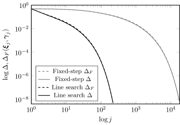
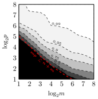
Refer to caption

Figure 2: Residual evolution of two exemplary runs of Alg. 1: with fixed steps μ𝝃,μ𝜸subscript𝜇𝝃subscript𝜇𝜸\mu_{\boldsymbol{\xi}},\mu_{\boldsymbol{\gamma}} (gray); with the line search updates given in (6.2) and (6.3) (black).
Refer to caption
(a) n=26,ρ=103formulae-sequence𝑛superscript26𝜌superscript103n=2^{6},\rho=10^{-3}
Refer to caption
(b) n=26,ρ=102formulae-sequence𝑛superscript26𝜌superscript102n=2^{6},\rho=10^{-2}
Refer to caption
(c) n=26,ρ=101formulae-sequence𝑛superscript26𝜌superscript101n=2^{6},\rho=10^{-1}
Refer to caption
(d) n=27,ρ=103formulae-sequence𝑛superscript27𝜌superscript103n=2^{7},\rho=10^{-3}
Refer to caption
(e) n=27,ρ=102formulae-sequence𝑛superscript27𝜌superscript102n=2^{7},\rho=10^{-2}
Refer to caption
(f) n=27,ρ=101formulae-sequence𝑛superscript27𝜌superscript101n=2^{7},\rho=10^{-1}
Refer to caption
(g) n=28,ρ=103formulae-sequence𝑛superscript28𝜌superscript103n=2^{8},\rho=10^{-3}
Refer to caption
(h) n=28,ρ=102formulae-sequence𝑛superscript28𝜌superscript102n=2^{8},\rho=10^{-2}
Refer to caption
(i) n=28,ρ=101formulae-sequence𝑛superscript28𝜌superscript101n=2^{8},\rho=10^{-1}
Figure 3: Empirical phase transition of (2.2) for increasing values of n𝑛n (top to bottom) and ρ𝜌\rho (left to right). We report the contours {0.25,0.5,0.75,0.9,0.95,0.99}0.250.50.750.90.950.99\{0.25,0.5,0.75,{0.9},0.95,0.99\} of the probability of exact recovery PTsubscriptPT\rm P_{T}. The superimposed curve in red corresponds to the sample complexity bound obtained in Theorem 3.1.

6.1 Step Size Updates

We begin our experiments by addressing a computational issue arising in Alg. 1, that is the choice of a step size for the gradient descent updates. Thm. 3.1 confirms that there is a scaling factor μ𝝃μ𝜸m𝒙2similar-to-or-equalssubscript𝜇𝝃subscript𝜇𝜸𝑚superscriptnorm𝒙2\tfrac{\mu_{\boldsymbol{\xi}}}{\mu_{\boldsymbol{\gamma}}}\simeq\tfrac{m}{\|{\boldsymbol{x}}\|^{2}} between the two fixed step sizes that ensures convergence to the global minimiser once we fix, e.g., a sufficiently small value for μ𝝃=μsubscript𝜇𝝃𝜇\mu_{\boldsymbol{\xi}}=\mu (and set μ𝜸subscript𝜇𝜸\mu_{\boldsymbol{\gamma}} accordingly).

However, in the practical application of our method we have found that updating the step sizes with the line searches reported in Alg. 1 is advantageous in terms of rate of convergence. Firstly, for some fixed values of (𝝃j,𝜸j)subscript𝝃𝑗subscript𝜸𝑗({\boldsymbol{\xi}}_{j},{\boldsymbol{\gamma}}_{j}) the line searches can be solved in closed form at iteration j𝑗j as

μ𝝃subscript𝜇𝝃\displaystyle\mu_{\boldsymbol{\xi}} l=1pdiag(𝜸j)𝑨l𝝃j,diag(𝜸)j𝑨l𝝃f(𝝃j,𝜸j)l=1pdiag(𝜸)j𝑨l𝝃f(𝝃j,𝜸j)2\displaystyle\coloneqq\frac{\sum^{p}_{l=1}\big{\langle}\operatorname{{diag}}({\boldsymbol{\gamma}}_{j}){\boldsymbol{A}}_{l}{\boldsymbol{\xi}}_{j},\operatorname{{diag}}({{\boldsymbol{\gamma}}})_{j}{\boldsymbol{A}}_{l}\boldsymbol{\nabla}_{\boldsymbol{\xi}}f({\boldsymbol{\xi}}_{j},{\boldsymbol{\gamma}}_{j})\big{\rangle}}{\sum^{p}_{l=1}\|\operatorname{{diag}}({{\boldsymbol{\gamma}}})_{j}{\boldsymbol{A}}_{l}\boldsymbol{\nabla}_{\boldsymbol{\xi}}f({\boldsymbol{\xi}}_{j},{\boldsymbol{\gamma}}_{j})\|^{2}} (6.2)
μ𝜸subscript𝜇𝜸\displaystyle\mu_{\boldsymbol{\gamma}} l=1pdiag(𝑨l𝝃j)𝜸j,diag(𝑨l𝝃j)𝜸f(𝝃j,𝜸j)l=1pdiag(𝑨l𝝃j)𝜸f(𝝃j,𝜸j)2absentsubscriptsuperscript𝑝𝑙1diagsubscript𝑨𝑙subscript𝝃𝑗subscript𝜸𝑗diagsubscript𝑨𝑙subscript𝝃𝑗subscriptsuperscriptbold-∇perpendicular-to𝜸𝑓subscript𝝃𝑗subscript𝜸𝑗subscriptsuperscript𝑝𝑙1superscriptnormdiagsubscript𝑨𝑙subscript𝝃𝑗subscriptsuperscriptbold-∇perpendicular-to𝜸𝑓subscript𝝃𝑗subscript𝜸𝑗2\displaystyle\coloneqq\frac{\sum^{p}_{l=1}\big{\langle}\operatorname{{diag}}({{\boldsymbol{A}}_{l}{\boldsymbol{\xi}}_{j}}){\boldsymbol{\gamma}}_{j},\operatorname{{diag}}({{\boldsymbol{A}}_{l}{\boldsymbol{\xi}}_{j}})\boldsymbol{\nabla}^{\perp}_{\boldsymbol{\gamma}}f({\boldsymbol{\xi}}_{j},{\boldsymbol{\gamma}}_{j})\big{\rangle}}{\sum^{p}_{l=1}\|\operatorname{{diag}}({{\boldsymbol{A}}_{l}{\boldsymbol{\xi}}_{j}})\boldsymbol{\nabla}^{\perp}_{\boldsymbol{\gamma}}f({\boldsymbol{\xi}}_{j},{\boldsymbol{\gamma}}_{j})\|^{2}} (6.3)

Equivalent formulas can be straightforwardly derived for Alg. 2. Note that (6.2) and (6.3) do not constitute a single exact line search, which would require solving another bilinear problem jointly with respect to the two step sizes. In fact, (6.2) and (6.3) are exact line searches when the signal- or the gain-domain iteration is fixed, in which case the two corresponding optimisation problems are convex and solved in closed-form; this strategy is, in all the simulations we carried out, a stable way of updating the step size that largely outperforms the choice of a fixed value for μ𝝃subscript𝜇𝝃\mu_{\boldsymbol{\xi}} and μ𝜸subscript𝜇𝜸\mu_{\boldsymbol{\gamma}}.

As an exemplary case, we randomly generated a typical problem instance with 𝒙𝕊n1𝒙superscript𝕊𝑛1{\boldsymbol{x}}\in\mathbb{S}^{n-1} and 𝒈𝟏m+𝟏mρ𝕊m1𝒈subscript1𝑚subscriptsuperscript1perpendicular-to𝑚𝜌subscriptsuperscript𝕊𝑚1{\boldsymbol{g}}\in\boldsymbol{1}_{m}+{{\boldsymbol{1}}^{\perp}_{m}}\cap\rho{\mathbb{S}}^{m-1}_{\infty}, setting n=256𝑛256n=256, m=64𝑚64m=64, ρ=0.99𝜌0.99\rho=0.99, and taking p=10𝑝10p=10 snapshots so that mpn+m=2𝑚𝑝𝑛𝑚2\tfrac{mp}{n+m}=2. Then, we ran Alg. 1 with either: (i)𝑖(i) μ𝝃=μ=104subscript𝜇𝝃𝜇superscript104\mu_{\boldsymbol{\xi}}=\mu=10^{-4}, μ𝜸=mμsubscript𝜇𝜸𝑚𝜇\mu_{\boldsymbol{\gamma}}=m\mu, or (ii)𝑖𝑖(ii) the step-size updates in (6.2),(6.3). The results are reported in Fig. 2 in terms of the decay of both Δ(𝝃j,𝜸j)Δsubscript𝝃𝑗subscript𝜸𝑗\Delta({\boldsymbol{\xi}}_{j},\boldsymbol{\gamma}_{j}) (solid lines) and ΔF(𝝃j,𝜸j)subscriptΔ𝐹subscript𝝃𝑗subscript𝜸𝑗\Delta_{F}({\boldsymbol{\xi}}_{j},\boldsymbol{\gamma}_{j}) (dashed lines), as a means to allow us to validate numerically the use of (2.5) instead of (2.4) to assess the convergence of our descent algorithm. Indeed, as expected Δ(𝝃j,𝜸j)Δsubscript𝝃𝑗subscript𝜸𝑗\Delta({\boldsymbol{\xi}}_{j},\boldsymbol{\gamma}_{j}) has the same decay as ΔF(𝝃j,𝜸j)subscriptΔ𝐹subscript𝝃𝑗subscript𝜸𝑗\Delta_{F}({\boldsymbol{\xi}}_{j},\boldsymbol{\gamma}_{j}) up to some constant factor. For what concerns the step-size choice, there is a clear advantage in choosing the rules in (6.2), (6.3) (black lines). For the given instance, convergence up to an objective value f(𝝃j,𝜸j)=108𝑓subscript𝝃𝑗subscript𝜸𝑗superscript108f({\boldsymbol{\xi}}_{j},{\boldsymbol{\gamma}}_{j})=10^{-8} is attained after j=220𝑗220j=220 iterations. On the other hand, the same problem instance using a fixed step size (with μ𝜇\mu chosen fairly by inspecting the values given by the update rules) does converge to the global minimiser with the same criterion, but requires j=17951𝑗17951j=17951 iterations, i.e., convergence is slower by two orders of magnitude in the number of iterates. With both step-size choices, the algorithm terminates with RMSEmax>86.49dBsubscriptRMSE86.49dB{\rm RMSE}_{\max}>86.49\,\mathrm{dB}. Thus, since convergence and accuracy do not ultimately depend on our step-size choice, we adopt the faster update rule for all further experiments. In addition, the step-size updates in (6.2), (6.3) did verify μ𝜸μ𝝃1msimilar-to-or-equalssubscript𝜇𝜸subscript𝜇𝝃1𝑚\tfrac{\mu_{\boldsymbol{\gamma}}}{\mu_{\boldsymbol{\xi}}}\simeq\textstyle\tfrac{1}{m} empirically in our experiments as the number of iterations j𝑗j increases.

Let us finally mention that analogue updates to (6.2),(6.3) are easily derived for Alg. 2 and consistently yield faster convergence than choosing fixed step sizes as those established in Thm. 4.1.

6.2 Empirical Phase Transition

To characterise the phase transition of (2.2), that is the transition between a region in which Alg. 1 successfully recovers (𝒙,𝒈)𝒙𝒈({\boldsymbol{x}},{\boldsymbol{g}}) with probability 111 and that in which it does with probability 00, we ran some extensive simulations by generating 256256256 random instances of (1.1) for each n={21,,28}𝑛superscript21superscript28n=\{2^{1},\ldots,2^{8}\}, probing the same range for m𝑚m and p𝑝p; we also varied for each configuration ρ={103,102,,1}𝜌superscript103superscript1021\rho=\{10^{-3},10^{-2},\ldots,1\}, generating 𝒈=𝟏m+𝒆𝒈subscript1𝑚𝒆{\boldsymbol{g}}=\boldsymbol{1}_{m}+{\boldsymbol{e}} with 𝒆𝒆{\boldsymbol{e}} drawn uniformly at random on 𝟏mρ𝕊m1subscriptsuperscript1perpendicular-to𝑚𝜌subscriptsuperscript𝕊𝑚1{{\boldsymbol{1}}^{\perp}_{m}}\cap\rho\,\mathbb{S}^{m-1}_{\infty}. Then we evaluated PT[max{𝒈¯𝒈𝒈,𝒙¯𝒙𝒙}<T]subscriptP𝑇delimited-[]norm¯𝒈𝒈norm𝒈norm¯𝒙𝒙norm𝒙𝑇{\rm P}_{T}\coloneqq\mathbb{P}\left[\textstyle\max\left\{\tfrac{\|\bar{{\boldsymbol{g}}}-{\boldsymbol{g}}\|}{\|{\boldsymbol{g}}\|},\tfrac{\|\bar{{\boldsymbol{x}}}-{\boldsymbol{x}}\|}{\|{\boldsymbol{x}}\|}\right\}<T\right] on the trials with threshold T=103𝑇superscript103T=10^{-3} chosen according to the stop criterion f(𝝃,𝜸)<108𝑓𝝃𝜸superscript108f({\boldsymbol{\xi}},{\boldsymbol{\gamma}})<10^{-8}. Of this large dataset we report the cases specified in Fig. 3, highlighting the contour lines of PTsubscriptP𝑇{\rm P}_{T}  for ρ={103,102,101}𝜌superscript103superscript102superscript101\rho=\{10^{-3},10^{-2},10^{-1}\} estimated from the outcome of our experiments as a function of log2msubscript2𝑚\log_{2}m and log2psubscript2𝑝\log_{2}p. There, we also plot a curve corresponding to the sample complexity bound that grants the verification of Thm. 3.1 (up to log\log factors), with the corresponding phase transition occurring at log2plog2(nm+1)similar-to-or-equalssubscript2𝑝subscript2𝑛𝑚1\log_{2}p\simeq\log_{2}\left(\tfrac{n}{m}+1\right). This curve matches the empirical phase transition up to a shift that is due to the required accuracy (i.e., the value of δ𝛿\delta) of the concentration inequalities. Moreover, we appreciate how an increase in ρ𝜌\rho does affect, albeit mildly, the requirements on (m,p)𝑚𝑝(m,p) for a successful recovery of (𝒙,𝒈)𝒙𝒈({\boldsymbol{x}},{\boldsymbol{g}}), and just as expected given its effect on the initialisation and the distance decay in (4.13).

6.3 Subspace Priors and the Effect of Coherence

Since Alg. 2 generalises Alg. 1 to known subspaces, we now focus on how the phase transition in Fig. 3 changes under subspace priors, as Thm. 4.1 suggests that the transition will occur when mpk+μmax2hgreater-than-or-equivalent-to𝑚𝑝𝑘superscriptsubscriptμ2mp\gtrsim k+\upmu_{\max}^{2}h (up to log\log factors). Indeed, the second term scales with μmax[1,mh]subscriptμ1𝑚\upmu_{\max}\in[1,\sqrt{\tfrac{m}{h}}] defined in (4.4), i.e., the larger μmaxsubscriptμ\upmu_{\max}, the farther the phase transition curve will be in the (log2m,log2p)subscript2𝑚subscript2𝑝(\log_{2}m,\log_{2}p) diagram.

As μmaxsubscriptμ\upmu_{\max} depends on the nature of the known subspace prior 𝑩(𝟏mm,𝑩)𝑩subscript1𝑚𝑚superscript𝑩perpendicular-to\boldsymbol{B}\coloneqq\big{(}\tfrac{\boldsymbol{1}_{m}}{\sqrt{m}},\ \boldsymbol{B}^{\perp}\big{)} in Def. 4.1, let us first fix 𝒁𝒁\boldsymbol{Z} by drawing its k𝑘k column vectors 𝒁i𝒩(𝟎n,𝑰n)similar-tosubscript𝒁𝑖𝒩subscript0𝑛subscript𝑰𝑛\boldsymbol{Z}_{i}\sim\mathcal{N}(\boldsymbol{0}_{n},\boldsymbol{I}_{n}) and running Gram-Schmidt orthonormalisation to comply with the hypothesis 𝒁𝒁=𝑰ksuperscript𝒁top𝒁subscript𝑰𝑘\boldsymbol{Z}^{\top}\boldsymbol{Z}=\boldsymbol{I}_{k}. Then, we compare three cases of 𝑩𝑩\boldsymbol{B} ranging between low and high coherence as follows; firstly, let us take 𝑩𝑪m𝑺Ωsuperscript𝑩perpendicular-tosubscript𝑪𝑚subscript𝑺Ω\boldsymbol{B}^{\perp}\coloneqq{\boldsymbol{C}}_{m}{\boldsymbol{S}}_{\Omega} with 𝑪msubscript𝑪𝑚{\boldsymbol{C}}_{m} an orthonormal basis of msuperscript𝑚\mathbb{R}^{m} specified below, and 𝑺Ωsubscript𝑺Ω\boldsymbol{S}_{\Omega} the selection operator at a randomly drawn index set Ω[m]:|Ω|=h1:Ωdelimited-[]𝑚Ω1\Omega\subset[m]:|\Omega|=h-1. We now proceed to detail the different choices of 𝑪msubscript𝑪𝑚\boldsymbol{C}_{m} and their coherence bounds.

  • Case 1 (DCT): we let 𝑪msubscript𝑪𝑚\boldsymbol{C}_{m} be the m𝑚m-dimensional type-II DCT matrix, i.e.,

    (𝑪m)i,j={1m,i[m],j=12mcos(π2m(j1)(2i1)),i[m],j[m]{1}.subscriptsubscript𝑪𝑚𝑖𝑗cases1𝑚formulae-sequence𝑖delimited-[]𝑚𝑗12𝑚𝜋2𝑚𝑗12𝑖1formulae-sequence𝑖delimited-[]𝑚𝑗delimited-[]𝑚1(\boldsymbol{C}_{m})_{i,j}=\begin{cases}\textstyle\tfrac{1}{\sqrt{m}},&i\in[m],j=1\\ \sqrt{\tfrac{2}{m}}\cos(\tfrac{\pi}{2m}(j-1)(2i-1)),&i\in[m],j\in[m]\setminus\{1\}\end{cases}.

    In this case, we pose that 1Ω1Ω1\notin\Omega to avoid selecting 𝟏mmsubscript1𝑚𝑚\tfrac{\boldsymbol{1}_{m}}{\sqrt{m}} as by construction it is already the first column of 𝑩𝑩\boldsymbol{B}. It is then simply estimated that

    μmax=mhmaxi[m]1m+jΩ2mcos2(π2m(j1)(2i1))<mh2h1m<2,subscriptμ𝑚subscript𝑖delimited-[]𝑚1𝑚subscript𝑗Ω2𝑚superscript2𝜋2𝑚𝑗12𝑖1𝑚21𝑚2\upmu_{\max}=\sqrt{\tfrac{m}{h}}\max_{i\in[m]}\sqrt{\textstyle\tfrac{1}{m}+\sum_{j\in\Omega}{\tfrac{2}{m}}\cos^{2}(\tfrac{\pi}{2m}(j-1)(2i-1))}<\sqrt{\tfrac{m}{h}}\sqrt{\tfrac{2h-1}{m}}<\sqrt{2},

    i.e., that this “DCT” case always attains relatively low coherence, similarly to the discrete Fourier transform (see [4, Sec. I-D]);

  • Case 2 (Id.): we let 𝑪m[𝑼𝑼]subscript𝑪𝑚matrix𝑼superscript𝑼perpendicular-to\boldsymbol{C}_{m}\coloneqq\begin{bmatrix}{\boldsymbol{U}}&\boldsymbol{U}^{\perp}\end{bmatrix}, where 𝑼[1m𝟏mmm1(11m1m𝟏m1)]𝑼matrix1𝑚subscript1𝑚𝑚𝑚1matrix11𝑚1𝑚subscript1𝑚1\boldsymbol{U}\coloneqq\begin{bmatrix}\textstyle\tfrac{1}{\sqrt{m}}\boldsymbol{1}_{m}&\sqrt{\tfrac{m}{m-1}}\begin{pmatrix}1-\textstyle\tfrac{1}{m}\\ -\textstyle\tfrac{1}{m}\boldsymbol{1}_{m-1}\end{pmatrix}\end{bmatrix} and 𝑼superscript𝑼perpendicular-to\boldsymbol{U}^{\perp} is an orthonormal basis for the null space of 𝑼superscript𝑼top\boldsymbol{U}^{\top} (again, obtained by the Gram-Schmidt process). We pose again 1Ω1Ω1\notin\Omega, and note that the resulting 𝑪msubscript𝑪𝑚\boldsymbol{C}_{m} resembles an identity matrix with a negative offset (hence the shorthand “Id.”). In fact, since the first row obtained this way always has only two non-zero elements, it is easily shown that 𝑩𝒄122=1m+(11m)2mm1=1subscriptsuperscriptnormsuperscript𝑩topsubscript𝒄1221𝑚superscript11𝑚2𝑚𝑚11\|\boldsymbol{B}^{\top}\boldsymbol{c}_{1}\|^{2}_{2}=\textstyle\tfrac{1}{m}+(1-\textstyle\tfrac{1}{m})^{2}{\tfrac{m}{m-1}}=1 which sets μmax=mhsubscriptμ𝑚\upmu_{\max}=\sqrt{\tfrac{m}{h}}. This choice attains the upper-bound for μmaxsubscriptμ\upmu_{\max}, and is thus expected to exhibit the worst-case phase transition;

  • Case 3 (Rand.): we let 𝑪m𝑼𝑽subscript𝑪𝑚𝑼𝑽\boldsymbol{C}_{m}\coloneqq{\boldsymbol{U}}\boldsymbol{V}, where 𝑼m×m1𝑼superscript𝑚𝑚1{\boldsymbol{U}}\in\mathbb{R}^{m\times m-1} is now an orthonormal basis for the null space of 𝟏msubscript1𝑚\boldsymbol{1}_{m} (again, obtained by the Gram-Schmidt process). We then apply a random rotation by 𝑽m1×h1𝑽superscript𝑚11\boldsymbol{V}\in\mathbb{R}^{m-1\times h-1} generated by drawing h11h-1 column vectors 𝑽j𝒩(𝟎m1,𝑰m1)similar-tosubscript𝑽𝑗𝒩subscript0𝑚1subscript𝑰𝑚1\boldsymbol{V}_{j}\sim\mathcal{N}(\boldsymbol{0}_{m-1},\boldsymbol{I}_{m-1}), orthogonalising them afterwards. This results in 𝑽superscript𝑽top\boldsymbol{V}^{\top} and 𝑪msubscriptsuperscript𝑪top𝑚\boldsymbol{C}^{\top}_{m} verifying the restricted isometry property. In particular, by [35, Lemma 3] it follows that the rows of 𝑩𝑩\boldsymbol{B} have norm 𝑩𝒄i1m+(1+δ)h1m2hmnormsuperscript𝑩topsubscript𝒄𝑖1𝑚1𝛿1𝑚less-than-or-similar-to2𝑚\|\boldsymbol{B}^{\top}\boldsymbol{c}_{i}\|\leq\textstyle\tfrac{1}{\sqrt{m}}+(1+\delta)\sqrt{\frac{h-1}{m}}\lesssim\sqrt{\tfrac{2h}{m}}, hence μmax2greater-than-or-equivalent-tosubscriptμ2\upmu_{\max}\gtrsim\sqrt{2} as in the “DCT” case.

With these three cases at hand, we may now run some simulations to assess how Alg. 2 actually performs on randomly generated instances of (4.1). To do so, we repeat the generation of Sec. 6.2 for n=28𝑛superscript28n=2^{8}, k=26𝑘superscript26k=2^{6}, varying h={24,25}superscript24superscript25h=\{2^{4},2^{5}\} and m={2log2h,,28}𝑚superscript2subscript2superscript28m=\{2^{\log_{2}h},\ldots,2^{8}\} since only mh𝑚m\geq h is meaningful. The resulting phase transitions at probability 0.90.90.9 are reported in Fig. 4. There, we can see that a large μmaxsubscriptμ\upmu_{\max} does have a negative effect on the phase transition for successful recovery, that is consistent with the result in Thm. 4.1.
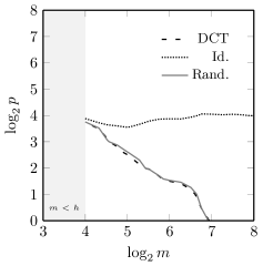
Refer to caption

(a) h=dim=24dimensionsuperscript24h=\dim\mathcal{B}=2^{4}

Refer to caption

(b) h=dim=25dimensionsuperscript25h=\dim\mathcal{B}=2^{5}
Figure 4: Phase transition of Alg. 2 at probability 0.90.90.9 for n=28𝑛superscript28n=2^{8}, k=26𝑘superscript26k=2^{6}, and three different cases of 𝑩𝑩\boldsymbol{B} (i.e., above each curve, the corresponding probability of successful recovery exceeds 0.90.90.9).

6.4 Noise Stability

Refer to caption

Figure 5: Performances of Alg. 1 in the presence of noise. This experiment details the exemplary case m=n=28,ρ=101formulae-sequence𝑚𝑛superscript28𝜌superscript101m=n=2^{8},\rho=10^{-1} for different values of p𝑝p; we report the average relative mean-square error as a function of the noise level σ𝜎\sigma.

As a numerical confirmation of the theory devised in Sec. 5 we run some numerical experiments to verify the effect of noise on the estimate obtained by Alg. 1, i.e., without subspace priors for simplicity. The simulations are carried out as follows: we generate 646464 instances101010This lower value is due to the fact that, when our algorithm does not converge, meeting the stop criterion requires a larger number of iterations due to the presence of noise. of (1.2), fixing n=m=28,ρ=101formulae-sequence𝑛𝑚superscript28𝜌superscript101n=m=2^{8},\rho=10^{-1} and varying p={21,,28}𝑝superscript21superscript28p=\{2^{1},\ldots,2^{8}\}. Moreover, we generate additive and bounded noise instances collected in a matrix 𝑵𝑵\boldsymbol{N} whose entries are drawn as νi,li.i.d.𝒩(0,1)subscriptsimilar-toi.i.d.subscript𝜈𝑖𝑙𝒩01\nu_{i,l}\sim_{\rm\textrm{i.i.d.}}\mathcal{N}(0,1) and normalised afterwards to meet a given σ=1mp𝑵F𝜎1𝑚𝑝subscriptnorm𝑵𝐹\sigma=\tfrac{1}{\sqrt{mp}}\|{\boldsymbol{N}}\|_{F}. This noise level value is then varied as σ={10,20,,80}dB𝜎102080dB\sigma=\{10,20,\ldots,80\}\,\mathrm{dB}. Since the objective function will reach a noise-dependent value, we change the stop criterion to the condition max{𝝃j+1𝝃j𝝃j,𝜸j+1𝜸j𝜸j}<106normsubscript𝝃𝑗1subscript𝝃𝑗normsubscript𝝃𝑗normsubscript𝜸𝑗1subscript𝜸𝑗normsubscript𝜸𝑗superscript106\max\left\{\tfrac{\|{\boldsymbol{\xi}}_{j+1}-{\boldsymbol{\xi}}_{j}\|}{\|{\boldsymbol{\xi}}_{j}\|},\tfrac{\|{\boldsymbol{\gamma}}_{j+1}-{\boldsymbol{\gamma}}_{j}\|}{\|{\boldsymbol{\gamma}}_{j}\|}\right\}<10^{-6}, terminating the algorithm and returning its best estimate up to the given tolerance. To extract a single figure of merit from the outcomes of this experiment, we compute the 𝔼RMSEmax𝔼subscriptRMSE\operatorname{{\mathbb{E}}}{\rm RMSE}_{\max} on our set of 646464 trials, with 𝔼𝔼\operatorname{{\mathbb{E}}} here denoting the sample average over the trials’ outcomes. The results after running Alg. 1 are reported in Fig. 5 and confirm the predicted graceful decay in the 𝔼RMSEmax𝔼subscriptRMSE\operatorname{{\mathbb{E}}}{\rm RMSE}_{\max} as a function of σ𝜎\sigma, i.e., the achieved relative mean-square error decreases linearly (in a loglog\log-\log scale) with the amount of noise injected into the model, as suggested from Thm. 5.1.

6.5 A Computational Imaging Example

We envision that our framework could be applied broadly to sensing systems where obtaining calibrated gains as formulated in our models is a critical issue. Generally speaking, whenever there are means to capture measurements of the type 𝑨l𝒙subscript𝑨𝑙𝒙{\boldsymbol{A}}_{l}{\boldsymbol{x}}, and whenever the sensors (antennas, pixels, nodes) assigned to capturing the output of this operation are subject to gain uncertainties, it is worth putting into account the presence of 𝒈𝒈{\boldsymbol{g}} and to calibrate the sensing system against it. Clearly, the main requirement is indeed the introduction of several random draws of the sensing matrices 𝑨l,l[p]subscript𝑨𝑙𝑙delimited-[]𝑝{\boldsymbol{A}}_{l},l\in[p] which, depending on m,n𝑚𝑛m,n and the presence of subspace priors, will allow for lower values of p𝑝p as shown by our main sample complexity results. As an example, one could consider an image formation model in which a source 𝒙𝒙{\boldsymbol{x}} illuminates a programmable medium, set to apply a sensing matrix 𝑨lsubscript𝑨𝑙{\boldsymbol{A}}_{l} and to capture the output of this operation by means of a focal plane array. The disturbance could then be regarded as uncalibrated fixed pattern noise on this sensor array, as stylised in Fig. 6, or in fact as any attenuation such as some “haze” affecting the sensor array in a multiplicative fashion. In fact, this type of issue could physically arise in imaging modalities where 𝑨lsubscript𝑨𝑙{\boldsymbol{A}}_{l} are random convolutions rather than sub-Gaussian random matrices, as anticipated before. With a due gap between the theory covered in this paper and the actual nature of the sensing operator, our algorithm is still practically applicable and will eventually converge once a sufficient amount of observations with random sensing matrices is collected.

To apply our result in a realistic computational imaging context, we assume that 𝒙𝒙{\boldsymbol{x}} is a n=128×128pixel𝑛128128pixeln=128\times 128\,\mathrm{pixel} monochromatic image acquired by an uncalibrated sensing device that implements (1.1) in which its m=64×64pixel𝑚6464pixelm=64\times 64\,\mathrm{pixel} sensor array has an unknown set of gains 𝒈Π+m𝒈subscriptsuperscriptΠ𝑚{\boldsymbol{g}}\in\Pi^{m}_{+}. This set of gains is specialised in two cases described hereafter. For the sake of this application example, we maintain 𝑨lsubscript𝑨𝑙{\boldsymbol{A}}_{l} comprised of i.i.d. rows 𝒂i,l𝒩(𝟎n,𝑰n)similar-tosubscript𝒂𝑖𝑙𝒩subscript0𝑛subscript𝑰𝑛\boldsymbol{a}_{i,l}\sim\mathcal{N}(\boldsymbol{0}_{n},\boldsymbol{I}_{n}).

Blind Calibration in Absence of Priors
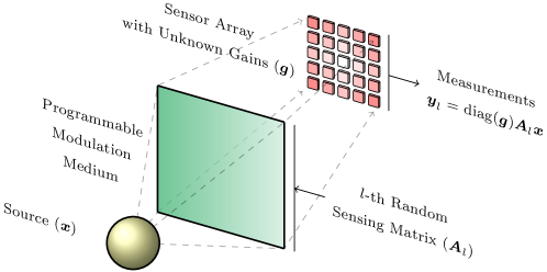
Refer to caption
Figure 6: A computational imaging model: our blind calibration framework entails the joint recovery of the source 𝒙𝒙{\boldsymbol{x}} and sensor gains 𝒈𝒈{\boldsymbol{g}} by exploiting multiple random sensing matrices 𝑨lsubscript𝑨𝑙{\boldsymbol{A}}_{l} (e.g.p𝑝p programmable random masks in a random convolution setup [15]). The intensity of 𝒈𝒈{\boldsymbol{g}} is represented in shades of red as a possible vignetting of the sensor array.


Refer to caption
(a) 𝒙𝒙{\boldsymbol{x}} (true signal).
Refer to caption
(b) 𝒙¯lssubscript¯𝒙ls\bar{{\boldsymbol{x}}}_{\rm ls} recovered by least squares with model error; RMSE=9.22dBRMSE9.22dB{\rm RMSE}=-9.22\,\mathrm{dB}.
Refer to caption
(c) 𝒙¯¯𝒙\bar{{\boldsymbol{x}}} recovered by Alg. 1; RMSE=149.96dBRMSE149.96dB{\rm RMSE}=-149.96\,\mathrm{dB}.
Refer to caption
(d) 𝒈𝒈{\boldsymbol{g}} (true sensor gains), ρ=0.99𝜌0.99\rho=0.99.
Refer to caption
(e) 𝒈¯¯𝒈\bar{{\boldsymbol{g}}} recovered by Alg. 1; RMSE=145.39dBRMSE145.39dB{\rm RMSE}=-145.39\,\mathrm{dB}.
Figure 7: A high-dimensional example of blind calibration for computational imaging. The unknown gains 𝒈𝒈{\boldsymbol{g}} (m=64×64pixel)𝑚6464pixel(m=64\times 64\,\mathrm{pixel}) and signal 𝒙𝒙{\boldsymbol{x}} (n=128×128pixel)𝑛128128pixel(n=128\times 128\,\mathrm{pixel}) are perfectly recovered with p=10𝑝10p=10 snapshots.


Refer to caption
(a) 𝒙𝒙{\boldsymbol{x}} (true signal)
Refer to caption
(b) 𝒙¯lssubscript¯𝒙ls\bar{{\boldsymbol{x}}}_{\rm ls} recovered by least squares with model error; RMSE=3.42dBRMSE3.42dB{\rm RMSE}=-3.42\,\mathrm{dB}.
Refer to caption
(c) 𝒙¯¯𝒙\bar{{\boldsymbol{x}}} recovered by Alg. 2; RMSE=138.84dBRMSE138.84dB{\rm RMSE}=-138.84\,\mathrm{dB}.
Refer to caption
(d) 𝒈𝒈{\boldsymbol{g}} (true sensor gains), ρ=0.99𝜌0.99\rho=0.99
Refer to caption
(e) 𝒈¯¯𝒈\bar{{\boldsymbol{g}}} recovered by Alg. 2; RMSE=144.99dBRMSE144.99dB{\rm RMSE}=-144.99\,\mathrm{dB}.
Figure 8: A high-dimensional example of blind calibration for computational imaging with subspace priors. The unknown gains 𝒈𝒈{\boldsymbol{g}} (m=64×64pixel)𝑚6464pixel(m=64\times 64\,\mathrm{pixel}) and signal 𝒙𝒙{\boldsymbol{x}} (n=128×128pixel)𝑛128128pixel(n=128\times 128\,\mathrm{pixel}) are perfectly recovered with p=1𝑝1p=1 snapshot, since they are described by known subspaces of dimension h=256256h=256 and k=2730𝑘2730k=2730, respectively.

In this first example we randomly draw the gains 𝒈Π+m𝒈subscriptsuperscriptΠ𝑚{\boldsymbol{g}}\in\Pi^{m}_{+} at random as 𝒈𝟏m+𝟏mρ𝕊m1𝒈subscript1𝑚subscriptsuperscript1perpendicular-to𝑚𝜌subscriptsuperscript𝕊𝑚1{\boldsymbol{g}}\in\boldsymbol{1}_{m}+{{\boldsymbol{1}}^{\perp}_{m}}\cap\rho\mathbb{S}^{m-1}_{\infty}, fixing ρ=0.99𝜌0.99\rho=0.99. We capture p=10𝑝10p=10 snapshots, again so that mpn+m=2𝑚𝑝𝑛𝑚2\tfrac{mp}{n+m}=2. By running Alg. 1 we obtain the results depicted in Fig. 7. The recovered (𝒙¯,𝒈¯)(𝒙,𝒈)¯𝒙¯𝒈𝒙𝒈(\bar{{\boldsymbol{x}}},\bar{{\boldsymbol{g}}})\approx({{\boldsymbol{x}}},{{\boldsymbol{g}}}) by solving (2.2) attains RMSEmax138.84dBsubscriptRMSE138.84dB{\rm RMSE}_{\max}\approx-138.84\,\mathrm{dB} in accordance with the stop criterion at f(𝝃k,𝜸k)<107𝑓subscript𝝃𝑘subscript𝜸𝑘superscript107f({\boldsymbol{\xi}}_{k},{\boldsymbol{\gamma}}_{k})<10^{-7}. Instead, by fixing 𝜸𝟏m𝜸subscript1𝑚{\boldsymbol{\gamma}}\coloneqq\boldsymbol{1}_{m} and solving (6.1) only with respect to 𝝃𝝃{\boldsymbol{\xi}}, the least-squares solution 𝒙¯lssubscript¯𝒙ls\bar{{\boldsymbol{x}}}_{\rm ls} reaches a RMSE𝒙¯𝒙𝒙9.22dBRMSEnorm¯𝒙𝒙norm𝒙9.22dB{\rm RMSE}\coloneqq\tfrac{\|\bar{{\boldsymbol{x}}}-{\boldsymbol{x}}\|}{\|{\boldsymbol{x}}\|}\approx-9.22\,\mathrm{dB}.

Blind Calibration with Subspace Priors

We now proceed to evaluate the effect of subspace priors on the same exemplary case, with 𝒙𝒙{\boldsymbol{x}} constructed so that it matches the known subspace prior 𝒙=𝒁𝒛𝒙𝒁𝒛{\boldsymbol{x}}={\boldsymbol{Z}}{\boldsymbol{z}}, where 𝒁𝒁{\boldsymbol{Z}} is a set of k=2730𝑘2730k=2730 basis elements of a two-dimensional Haar orthonormal wavelet basis in nsuperscript𝑛\mathbb{R}^{n}. Moreover, we generate the gains with a subspace prior that entails 𝒈=𝑩𝒃𝒈𝑩𝒃{\boldsymbol{g}}={\boldsymbol{B}}{\boldsymbol{b}}, where 𝑩𝑩{\boldsymbol{B}} is a set of h=256256h=256 basis elements of a two-dimensional discrete cosine transform basis in msuperscript𝑚\mathbb{R}^{m}, including the DC component as its first column. The vector 𝒆=𝑩𝒃𝒆superscript𝑩perpendicular-tosuperscript𝒃perpendicular-to{\boldsymbol{e}}={\boldsymbol{B}}^{\perp}{\boldsymbol{b}}^{\perp} is drawn with a low-pass profile as shown in Fig. 8 as a means to simulate a structured model for the gains. We also fix 𝒆=ρsubscriptnorm𝒆𝜌\|{\boldsymbol{e}}\|_{\infty}=\rho on the generated profile, with ρ=0.99𝜌0.99\rho=0.99. Substantially, what changes with respect to the previous experiment is the introduction of a known subspace prior for the signal and gains, both benefiting from such a low-dimensional model. Due to this additional prior we can take a single snapshot (i.e.p=1𝑝1p=1) provided that 𝑩𝑩\boldsymbol{B} has sufficiently low μmaxsubscriptμ\upmu_{\max} and that m>c(k+μmax2h)log2(m(n+1))𝑚𝑐𝑘subscriptsuperscriptμ2superscript2𝑚𝑛1m>c({k+\upmu^{2}_{\max}h})\,\log^{2}(m(n+1)) for some c>0𝑐0c>0, i.e.m𝑚m must exceed, up to some constant and log\log factors, k+μmax2h𝑘subscriptsuperscriptμ2{k+\upmu^{2}_{\max}h}.

Then, by running Alg. 2 we obtain the results depicted in Fig. 8. The recovered (𝒙¯,𝒈¯)(𝒁𝒛¯,𝑩𝒃¯)(𝒙,𝒈)¯𝒙¯𝒈𝒁¯𝒛𝑩¯𝒃𝒙𝒈(\bar{{\boldsymbol{x}}},\bar{{\boldsymbol{g}}})\coloneqq(\boldsymbol{Z}\bar{\boldsymbol{z}},\boldsymbol{B}\bar{{\boldsymbol{b}}})\approx({{\boldsymbol{x}}},{{\boldsymbol{g}}}) achieves a RMSEmax=138.84dBsubscriptRMSE138.84dB{\rm RMSE}_{\max}=-138.84\,\mathrm{dB} in accordance with the stop criterion at fs(𝜻k,𝜷k)<107superscript𝑓ssubscript𝜻𝑘subscript𝜷𝑘superscript107f^{\rm s}(\boldsymbol{\zeta}_{k},{\boldsymbol{\beta}}_{k})<10^{-7}. Instead, by fixing 𝜷(m,𝟎m)𝜷superscript𝑚superscriptsubscript0𝑚toptop{\boldsymbol{\beta}}\coloneqq(\sqrt{m},\boldsymbol{0}_{m}^{\top})^{\top} and solving (6.1) when setting 𝝃=𝒁𝜻𝝃𝒁𝜻\boldsymbol{\xi}=\boldsymbol{Z}\boldsymbol{\zeta} and with respect to 𝜻𝜻\boldsymbol{\zeta} yields a least-squares solution 𝒛¯lssubscript¯𝒛ls\bar{\boldsymbol{z}}_{\rm ls} that reaches a RMSE𝒛¯ls𝒛𝒛3.42dBRMSEnormsubscript¯𝒛ls𝒛norm𝒛3.42dB{\rm RMSE}\coloneqq\tfrac{\|\bar{\boldsymbol{z}}_{\rm ls}-\boldsymbol{z}\|}{\|\boldsymbol{z}\|}\approx-3.42\,\mathrm{dB}.

We have therefore seen how the algorithms devised in this paper work on practical instances of the uncalibrated sensing models studied in this paper. The application of this bilinear inverse problem in the solution of physical instances of (1.1) or (1.2) is an open subject for future developments.

7 Conclusion

We presented and solved a non-convex formulation of blind calibration in the specific, yet important case of linear random sensing models affected by unknown gains. In absence of a priori structure on the signal and gains, we have devised and analysed a descent algorithm based on a simple projected gradient descent. In this case, our main results have shown that provable convergence of the algorithm can be achieved at a rate mp𝑚𝑝mp == 𝒪((m+n){\mathcal{O}}\big{(}(m+n) log2(m(p+n)))\log^{2}(m(p+n))\big{)} that is linear (up to log\log factors) with respect to the number of unknowns in this bilinear inverse problem. Similarly, using a subspace prior on both the signal and gains, a straightforward extension of the previous descent algorithm into Alg. 2 proved that the sample complexity ensuring convergence in this setting is mp𝑚𝑝mp == 𝒪((k+μmax2h){\mathcal{O}}\big{(}(k+\upmu^{2}_{\max}h) log2(m(p+n)))\log^{2}(m(p+n))\big{)}, leading to a worst-case value of mp𝑚𝑝mp == 𝒪((k+m){\mathcal{O}}\big{(}(k+m) log2(m(p+n)))\log^{2}(m(p+n))\big{)} when 𝑩𝑩\boldsymbol{B} achieves maximum coherence μmax=mhsubscriptμ𝑚\upmu_{\max}=\sqrt{\tfrac{m}{h}}.

We envision that our results could be extended to the case of complex gains (i.e.𝒈m𝒈superscript𝑚{\boldsymbol{g}}\in\mathbb{C}^{m}) and complex sensing operators 𝑨lsubscript𝑨𝑙\boldsymbol{A}_{l} by means of Wirtinger calculus (up to redefining our bounded subscript\ell_{\infty}-norm assumption made throughout this paper). Another important extension is the adaptation of Alg. 2 to enforce the sparsity of 𝒙𝒙{\boldsymbol{x}} (or 𝒈𝒈{\boldsymbol{g}}, although this may not be verified in practice). We explored numerically this possibility in [19]. By using sparsity we expect a reduction of the sample complexity that is similar to the subspace case, but without using such strong assumptions as prior information on a fixed, known tight frame 𝒁𝒁\boldsymbol{Z} in whose span 𝒙𝒙{\boldsymbol{x}} must lie.

Finally, our general technique is in line with the surge of new results on non-convex problems with linear, bilinear or quadratic random models. In fact, the core principle underlying this work is that, as several random instances of the same non-convex problem are taken, we approach its behaviour in expectation which, as previously discussed, is significantly more benign than the non-asymptotic case. This is an extremely general approach that could be applied to very different models than the ones we discussed.

Appendices

We now provide arguments to support the main results in this paper. Unless otherwise noted, the proofs are first given for the known subspace case discussed in Sec. 4. In fact, the proofs for our statements in absence of priors (i.e., as discussed throughout Sec. 2) are particular cases of the corresponding statements in the known subspace case (Sec. 4).

A Technical Tools

We begin by introducing some technical results used in the following proofs. Hereafter, we recall that 𝒂n𝒂superscript𝑛\boldsymbol{a}\in\mathbb{R}^{n} denotes a sub-Gaussian and isotropic random vector comprised of r.v.’s aiiidXsubscriptsimilar-toiidsubscript𝑎𝑖𝑋a_{i}\sim_{\rm iid}X, i[n]𝑖delimited-[]𝑛i\in[n], with X𝑋X a centred and unit-variance sub-Gaussian r.v. with sub-Gaussian norm Xψ2=α>0subscriptnorm𝑋subscript𝜓2𝛼0\|X\|_{\psi_{2}}=\alpha>0.

Proposition A.1 (Concentration Bound on 2subscript2\ell_{2}-Norm of sub-Gaussian r.v.’s).

Let 𝐚ii.i.d.𝐚subscriptsimilar-toi.i.d.subscript𝐚𝑖𝐚\boldsymbol{a}_{i}\sim_{\textrm{i.i.d.}}\boldsymbol{a} be a set of q2𝑞2q\geq 2 i.i.d. sub-Gaussian random vectors. There exists a value ϑ>1italic-ϑ1\vartheta>1 only depending on α𝛼\alpha such that, provided ntlogqgreater-than-or-equivalent-to𝑛𝑡𝑞n\gtrsim t\log q for some t1𝑡1t\geq 1, the event

max{maxi[q]𝒂i2ϑn},subscriptsubscript𝑖delimited-[]𝑞superscriptnormsubscript𝒂𝑖2italic-ϑ𝑛\displaystyle\mathcal{E}_{\max}\coloneqq\big{\{}\max_{i\in[q]}\|\boldsymbol{a}_{i}\|^{2}\leq\vartheta n\big{\}}, (A.1)

occurs with probability exceeding 12qt12superscript𝑞𝑡1-2q^{-t}.

Proof of Prop. A.1.

Since all 𝒂i𝒂similar-tosubscript𝒂𝑖𝒂\boldsymbol{a}_{i}\sim\boldsymbol{a} are comprised of i.i.d. sub-Gaussian r.v.’s with sub-Gaussian norm α𝛼\alpha, then 𝒂i2superscriptnormsubscript𝒂𝑖2\|\boldsymbol{a}_{i}\|^{2} can be bounded by standard concentration inequalities [14, Cor. 5.17]. In detail, since 𝒂i2superscriptnormsubscript𝒂𝑖2\|\boldsymbol{a}_{i}\|^{2}, i[q]𝑖delimited-[]𝑞i\in[q] are sub-exponential variables with 𝔼𝒂i2=n𝔼superscriptnormsubscript𝒂𝑖2𝑛\mathbb{E}\|\boldsymbol{a}_{i}\|^{2}=n, there exists some c>0𝑐0c>0 such that the probability of the complementary event is bounded as

[maxc]q[𝒂2>(1+ϑ)n]q[|𝒂2n|>ϑn]<2exp(logqcmin{ϑ2α4,ϑα2}n),delimited-[]superscriptsubscriptc𝑞delimited-[]superscriptnorm𝒂21superscriptitalic-ϑ𝑛𝑞delimited-[]superscriptnorm𝒂2𝑛superscriptitalic-ϑ𝑛2𝑞𝑐superscriptitalic-ϑ2superscript𝛼4superscriptitalic-ϑsuperscript𝛼2𝑛\mathbb{P}[\mathcal{E}_{\max}^{\rm c}]\leq q\,\mathbb{P}\big{[}\|\boldsymbol{a}\|^{2}>(1+\vartheta^{\prime})n\big{]}\leq q\,\mathbb{P}\big{[}\big{|}\|\boldsymbol{a}\|^{2}-n\big{|}>\vartheta^{\prime}n\big{]}<2\exp\big{(}\log q-c\min\big{\{}\tfrac{\vartheta^{\prime 2}}{\alpha^{4}},\tfrac{\vartheta^{\prime}}{\alpha^{2}}\big{\}}n\big{)},

with ϑϑ1>0superscriptitalic-ϑitalic-ϑ10\vartheta^{\prime}\coloneqq\vartheta-1>0. Therefore, provided ϑmin(ϑ,α2)>2cα4superscriptitalic-ϑsuperscriptitalic-ϑsuperscript𝛼22𝑐superscript𝛼4\vartheta^{\prime}\min(\vartheta^{\prime},\alpha^{2})>\tfrac{2}{c}\alpha^{4} (which leads to a lower bound on ϑitalic-ϑ\vartheta only depending on α𝛼\alpha) we find [maxc]<2qtdelimited-[]superscriptsubscriptc2superscript𝑞𝑡\mathbb{P}[\mathcal{E}_{\max}^{\rm c}]<2q^{-t} when ntlogq𝑛𝑡𝑞n\geq t\log q for t1𝑡1t\geq 1. ∎

We now introduce a proposition that provides a concentration inequality for a weighted sum of matrices (these being functions of i.i.d. sub-Gaussian random vectors) that will be frequently used in the following proofs. This result is related to finding a bound for the spectral norm of the residual between a covariance matrix and its sample estimate [36] in the special case where a weighting affects the computation, and where both the corresponding weights and the vectors to which this residual applies are assumed to lie in known subspaces.

Proposition A.2 (Weighted Covariance Concentration in Subspaces).

Consider a set of q𝑞q random vectors 𝐚ii.i.d.𝐚subscriptsimilar-toi.i.d.subscript𝐚𝑖𝐚\boldsymbol{a}_{i}\sim_{\textrm{i.i.d.}}\boldsymbol{a}, and two subspaces 𝒵n𝒵superscript𝑛\mathcal{Z}\subset\mathbb{R}^{n} and 𝒮q𝒮superscript𝑞\mathcal{S}\subset\mathbb{R}^{q} of dimensions kn𝑘𝑛k\leq n and sq𝑠𝑞s\leq q, respectively. Let 𝐙n×k𝐙superscript𝑛𝑘\boldsymbol{Z}\in\mathbb{R}^{n\times k} be an orthonormal basis of 𝒵𝒵\mathcal{Z}, i.e.𝐙𝐙=𝐈ksuperscript𝐙top𝐙subscript𝐈𝑘\boldsymbol{Z}^{\top}\boldsymbol{Z}=\boldsymbol{I}_{k}. Given δ(0,1)𝛿01\delta\in(0,1), t1𝑡1t\geq 1, provided ntlog(q)greater-than-or-equivalent-to𝑛𝑡𝑞n\gtrsim t\log(q) and

qδ2(k+s)log(nδ),greater-than-or-equivalent-to𝑞superscript𝛿2𝑘𝑠𝑛𝛿\textstyle q\gtrsim\delta^{-2}(k+s)\log\big{(}\frac{n}{\delta}\big{)},

with probability exceeding

1Cexp(cδ2q)qt1𝐶𝑐superscript𝛿2𝑞superscript𝑞𝑡1-C\exp(-c\delta^{2}q)-q^{-t}

for some C,c>0𝐶𝑐0C,c>0 depending only on α𝛼\alpha, we have for all 𝐰𝒮𝐰𝒮\boldsymbol{w}\in\mathcal{S}

1qi=1qwi𝒁(𝒂i𝒂i𝑰n)𝒁δ𝒘.norm1𝑞superscriptsubscript𝑖1𝑞subscript𝑤𝑖superscript𝒁topsubscript𝒂𝑖subscriptsuperscript𝒂top𝑖subscript𝑰𝑛𝒁𝛿subscriptnorm𝒘\big{\|}\textstyle\tfrac{1}{q}\,\textstyle\sum_{i=1}^{q}w_{i}\boldsymbol{Z}^{\top}(\boldsymbol{a}_{i}\boldsymbol{a}^{\top}_{i}-\boldsymbol{I}_{n})\boldsymbol{Z}\big{\|}\leq\delta\,\|{\boldsymbol{w}}\|_{\infty}. (A.2)
Proof of Prop. A.2.

Note that by the assumptions on the r.v.’s aijsubscript𝑎𝑖𝑗a_{ij}, i[q]𝑖delimited-[]𝑞i\in[q], j[n]𝑗delimited-[]𝑛j\in[n] we have that the random vectors 𝒂isubscript𝒂𝑖\boldsymbol{a}_{i}, i[q]𝑖delimited-[]𝑞i\in[q] are i.i.d. centred (𝔼𝒂i=𝟎n𝔼subscript𝒂𝑖subscript0𝑛\operatorname{{\mathbb{E}}}\boldsymbol{a}_{i}=\boldsymbol{0}_{n}) and isotropic (𝔼𝒂i𝒂i=𝑰n𝔼subscript𝒂𝑖superscriptsubscript𝒂𝑖topsubscript𝑰𝑛\operatorname{{\mathbb{E}}}\boldsymbol{a}_{i}\boldsymbol{a}_{i}^{\top}=\boldsymbol{I}_{n}). By homogeneity of (A.2) it suffices to show the probability that the event

{1qi=1qwi𝒁(𝒂i𝒂i𝑰n)𝒁δ}norm1𝑞superscriptsubscript𝑖1𝑞subscript𝑤𝑖superscript𝒁topsubscript𝒂𝑖subscriptsuperscript𝒂top𝑖subscript𝑰𝑛𝒁𝛿\displaystyle\mathcal{E}\coloneqq\big{\{}\big{\|}\textstyle\tfrac{1}{q}\,\textstyle\sum_{i=1}^{q}w_{i}\boldsymbol{Z}^{\top}(\boldsymbol{a}_{i}\boldsymbol{a}^{\top}_{i}-\boldsymbol{I}_{n})\boldsymbol{Z}\big{\|}\leq\delta\big{\}}

holds for all 𝒘𝒮𝕊q1𝒘𝒮subscriptsuperscript𝕊𝑞1{\boldsymbol{w}}\in\mathcal{S}\cap\mathbb{S}^{q-1}_{\infty}.

Step 1: Concentration  Let us first observe that, since the rank-one matrices 𝒂i𝒂i,i[q]subscript𝒂𝑖subscriptsuperscript𝒂top𝑖𝑖delimited-[]𝑞\boldsymbol{a}_{i}\boldsymbol{a}^{\top}_{i},i\in[q] are symmetric and 𝒁𝒁=𝑰ksuperscript𝒁top𝒁subscript𝑰𝑘\boldsymbol{Z}^{\top}\boldsymbol{Z}=\boldsymbol{I}_{k},

1qi=1qwi𝒁(𝒂i𝒂i𝑰n)𝒁norm1𝑞superscriptsubscript𝑖1𝑞subscript𝑤𝑖superscript𝒁topsubscript𝒂𝑖subscriptsuperscript𝒂top𝑖subscript𝑰𝑛𝒁\displaystyle\big{\|}\textstyle\tfrac{1}{q}\,\textstyle\sum_{i=1}^{q}w_{i}\boldsymbol{Z}^{\top}(\boldsymbol{a}_{i}\boldsymbol{a}^{\top}_{i}-\boldsymbol{I}_{n})\boldsymbol{Z}\big{\|} =sup𝒛𝕊2k11q|i=1qwi(𝒛𝒁𝒂i𝒂i𝒁𝒛𝒁𝒛2)|absentsubscriptsupremum𝒛superscriptsubscript𝕊2𝑘11𝑞superscriptsubscript𝑖1𝑞subscript𝑤𝑖superscript𝒛topsuperscript𝒁topsubscript𝒂𝑖subscriptsuperscript𝒂top𝑖𝒁𝒛superscriptnorm𝒁𝒛2\displaystyle=\sup_{\boldsymbol{z}\in{\mathbb{S}}_{2}^{k-1}}\textstyle\tfrac{1}{q}\,\big{|}\textstyle\sum_{i=1}^{q}w_{i}(\boldsymbol{z}^{\top}\boldsymbol{Z}^{\top}\boldsymbol{a}_{i}\boldsymbol{a}^{\top}_{i}\boldsymbol{Z}\boldsymbol{z}-\|\boldsymbol{Z}\boldsymbol{z}\|^{2})\big{|}
=sup𝒖𝒁𝕊2k11q|i=1qwi(𝒖𝒂i𝒂i𝒖𝒖2)|absentsubscriptsupremum𝒖𝒁superscriptsubscript𝕊2𝑘11𝑞superscriptsubscript𝑖1𝑞subscript𝑤𝑖superscript𝒖topsubscript𝒂𝑖subscriptsuperscript𝒂top𝑖𝒖superscriptnorm𝒖2\displaystyle=\sup_{{\boldsymbol{u}}\in\boldsymbol{Z}{\mathbb{S}}_{2}^{k-1}}\textstyle\tfrac{1}{q}\,\big{|}\textstyle\sum_{i=1}^{q}w_{i}({\boldsymbol{u}}^{\top}\boldsymbol{a}_{i}\boldsymbol{a}^{\top}_{i}{\boldsymbol{u}}-\|{\boldsymbol{u}}\|^{2})\big{|}
=sup𝒖𝒁𝕊2n11q|i=1q(Vi(𝒖)wi𝒖2)|,absentsubscriptsupremum𝒖𝒁superscriptsubscript𝕊2𝑛11𝑞superscriptsubscript𝑖1𝑞subscript𝑉𝑖𝒖subscript𝑤𝑖superscriptnorm𝒖2\displaystyle=\sup_{{\boldsymbol{u}}\in\boldsymbol{Z}\mathbb{S}_{2}^{n-1}}\textstyle\tfrac{1}{q}\,\big{|}\textstyle\sum_{i=1}^{q}(V_{i}({\boldsymbol{u}})-w_{i}\|{\boldsymbol{u}}\|^{2})\big{|},

with Vi(𝒖)wi(𝒂i𝒖)2,i[q]formulae-sequencesubscript𝑉𝑖𝒖subscript𝑤𝑖superscriptsubscriptsuperscript𝒂top𝑖𝒖2𝑖delimited-[]𝑞V_{i}({\boldsymbol{u}})\coloneqq w_{i}(\boldsymbol{a}^{\top}_{i}{\boldsymbol{u}})^{2},i\in[q] and 𝔼Vi(𝒖)=wi𝒖2𝔼subscript𝑉𝑖𝒖subscript𝑤𝑖superscriptnorm𝒖2\mathbb{E}V_{i}({\boldsymbol{u}})=w_{i}\|{\boldsymbol{u}}\|^{2}.

Let us fix 𝒖𝒁𝕊2k1𝒖𝒁subscriptsuperscript𝕊𝑘12{\boldsymbol{u}}\in\boldsymbol{Z}\mathbb{S}^{k-1}_{2} and 𝒘𝒮𝒮𝕊q1𝒘superscript𝒮𝒮superscriptsubscript𝕊𝑞1{\boldsymbol{w}}\in\mathcal{S}^{*}\coloneqq\mathcal{S}\cap\mathbb{S}_{\infty}^{q-1} (which implies |wi|1,i[q]formulae-sequencesubscript𝑤𝑖1𝑖delimited-[]𝑞|w_{i}|\leq 1,i\in[q]). Firstly, we observe that Vi(𝒖)subscript𝑉𝑖𝒖V_{i}({\boldsymbol{u}}) is a sub-exponential r.v. since each 𝒂isubscript𝒂𝑖\boldsymbol{a}_{i} is formed by sub-Gaussian r.v.’s, so we can bound the sub-exponential norm

Vi(𝒖)ψ1=|wi|(𝒂i𝒖)2ψ12|wi|𝒂i𝒖ψ22α2,subscriptnormsubscript𝑉𝑖𝒖subscript𝜓1subscript𝑤𝑖subscriptnormsuperscriptsuperscriptsubscript𝒂𝑖top𝒖2subscript𝜓12subscript𝑤𝑖subscriptsuperscriptnormsuperscriptsubscript𝒂𝑖top𝒖2subscript𝜓2less-than-or-similar-tosuperscript𝛼2\displaystyle\|V_{i}({\boldsymbol{u}})\|_{\psi_{1}}=|w_{i}|\|(\boldsymbol{a}_{i}^{\top}{\boldsymbol{u}})^{2}\|_{\psi_{1}}\leq 2|w_{i}|\|\boldsymbol{\boldsymbol{a}}_{i}^{\top}{\boldsymbol{u}}\|^{2}_{\psi_{2}}\lesssim\alpha^{2},

where we used the fact that Vψ22V2ψ12Vψ22subscriptsuperscriptnorm𝑉2subscript𝜓2subscriptnormsuperscript𝑉2subscript𝜓12subscriptsuperscriptnorm𝑉2subscript𝜓2\|V\|^{2}_{\psi_{2}}\leq\|V^{2}\|_{\psi_{1}}\leq 2\|V\|^{2}_{\psi_{2}} for any r.v. V𝑉V [14, Lemma 5.14] and that, given any 𝘃𝕊2n1𝘃superscriptsubscript𝕊2𝑛1\boldsymbol{\mathsf{v}}\in\mathbb{S}_{2}^{n-1}, 𝒂i𝘃ψ22𝘃2Xψ22α2less-than-or-similar-tosubscriptsuperscriptnormsubscriptsuperscript𝒂top𝑖𝘃2subscript𝜓2superscriptnorm𝘃2subscriptsuperscriptnorm𝑋2subscript𝜓2less-than-or-similar-tosuperscript𝛼2\|\boldsymbol{a}^{\top}_{i}\boldsymbol{\mathsf{v}}\|^{2}_{\psi_{2}}\lesssim\|\boldsymbol{\mathsf{v}}\|^{2}\|X\|^{2}_{\psi_{2}}\lesssim\alpha^{2} by the rotational invariance of 𝒂isubscript𝒂𝑖\boldsymbol{a}_{i} [14, Lemma 5.9]. Thus, the r.v. Vi=1qVi(𝒖)𝑉superscriptsubscript𝑖1𝑞subscript𝑉𝑖𝒖V\coloneqq\textstyle\sum_{i=1}^{q}V_{i}({\boldsymbol{u}}) is in turn a sum of sub-exponential variables that concentrates around 𝔼V=i=1qwi𝒖2𝔼𝑉superscriptsubscript𝑖1𝑞subscript𝑤𝑖superscriptnorm𝒖2\operatorname{{\mathbb{E}}}V=\textstyle\sum_{i=1}^{q}w_{i}\|{\boldsymbol{u}}\|^{2}, i.e., for some c>0𝑐0c>0 and δ(0,1)𝛿01\delta\in(0,1), applying [14, Cor. 5.17] yields

[|V𝔼V|>δq]<2exp(cqmin(δ2α4,δα2))<2exp(cqδ2α41+α2)<2exp(cαδ2q),delimited-[]𝑉𝔼𝑉𝛿𝑞2𝑐𝑞superscript𝛿2superscript𝛼4𝛿superscript𝛼22𝑐𝑞superscript𝛿2superscript𝛼41superscript𝛼22subscript𝑐𝛼superscript𝛿2𝑞\displaystyle\textstyle\mathbb{P}[|V-\operatorname{{\mathbb{E}}}V|>\delta q]<2\exp\big{(}-cq\min(\tfrac{\delta^{2}}{\alpha^{4}},\tfrac{\delta}{\alpha^{2}})\big{)}<2\exp\big{(}-cq\tfrac{\delta^{2}\alpha^{-4}}{1+\alpha^{-2}}\big{)}<2\exp\big{(}-c_{\alpha}\delta^{2}q\big{)},

for some cα>0subscript𝑐𝛼0c_{\alpha}>0 depending only on α𝛼\alpha. Thus, with probability exceeding 12exp(cαδ2q)12subscript𝑐𝛼superscript𝛿2𝑞1-2\exp(-c_{\alpha}\delta^{2}q), the event

1q|i=1q(Vi(𝒖)wi𝒖2)|δ1𝑞superscriptsubscript𝑖1𝑞subscript𝑉𝑖𝒖subscript𝑤𝑖superscriptnorm𝒖2𝛿\textstyle\tfrac{1}{q}\big{|}\textstyle\sum_{i=1}^{q}(V_{i}({\boldsymbol{u}})-w_{i}\|{\boldsymbol{u}}\|^{2})\big{|}\leq\delta (A.3)

holds for some fixed 𝒖𝕊2n1,𝒘𝒮formulae-sequence𝒖subscriptsuperscript𝕊𝑛12𝒘superscript𝒮{\boldsymbol{u}}\in\mathbb{S}^{n-1}_{2},{\boldsymbol{w}}\in\mathcal{S}^{*}.

Step 2: Covering  To obtain a uniform result we resort to a covering argument. Given two radii ϵ,ϵ>0italic-ϵsuperscriptitalic-ϵ0\epsilon,\epsilon^{\prime}>0 to be fixed later, let us take an ϵitalic-ϵ\epsilon-net 𝒩ϵsubscript𝒩italic-ϵ\mathcal{N}_{\epsilon} of 𝒁𝔹2k𝒁subscriptsuperscript𝔹𝑘2\boldsymbol{Z}\,\mathbb{B}^{k}_{2} (i.e., with respect to 𝒖𝒖{\boldsymbol{u}}) and another ϵsuperscriptitalic-ϵ\epsilon^{\prime}-net 𝒲ϵsubscript𝒲superscriptitalic-ϵ\mathcal{W}_{\epsilon^{\prime}} of 𝒮𝔹q𝒮subscriptsuperscript𝔹𝑞\mathcal{S}\cap\mathbb{B}^{q}_{\infty}. Noting that 𝒁𝕊2k1𝒁𝔹2k𝒁subscriptsuperscript𝕊𝑘12𝒁subscriptsuperscript𝔹𝑘2\boldsymbol{Z}\,\mathbb{S}^{k-1}_{2}\subset\boldsymbol{Z}\,\mathbb{B}^{k}_{2} and 𝒮𝒮𝔹qsuperscript𝒮𝒮subscriptsuperscript𝔹𝑞\mathcal{S}^{*}\subset\mathcal{S}\cap\mathbb{B}^{q}_{\infty}, 𝒩ϵsubscript𝒩italic-ϵ\mathcal{N}_{\epsilon} and 𝒲ϵsubscript𝒲superscriptitalic-ϵ\mathcal{W}_{\epsilon^{\prime}} are also the corresponding nets of 𝒁𝕊2k1𝒁subscriptsuperscript𝕊𝑘12\boldsymbol{Z}\,\mathbb{S}^{k-1}_{2} and 𝒮superscript𝒮\mathcal{S}^{*}, respectively. Since 𝒁𝔹2k𝒁subscriptsuperscript𝔹𝑘2\boldsymbol{Z}\,\mathbb{B}^{k}_{2} is isomorphic to 𝔹2ksubscriptsuperscript𝔹𝑘2\mathbb{B}^{k}_{2}, a standard geometric argument provides that |𝒩ϵ|(1+2ϵ)k(3ϵ)ksubscript𝒩italic-ϵsuperscript12italic-ϵ𝑘superscript3italic-ϵ𝑘|\mathcal{N}_{\epsilon}|\leq(1+\tfrac{2}{\epsilon})^{k}\leq(\tfrac{3}{\epsilon})^{k} [37]. Moreover, given an orthonormal basis 𝑺q×s𝑺superscript𝑞𝑠\boldsymbol{S}\in\mathbb{R}^{q\times s} of 𝒮q𝒮superscript𝑞\mathcal{S}\subset\mathbb{R}^{q}, since 𝑺,𝑺\|\cdot\|_{\boldsymbol{S},\infty}\coloneqq\|\boldsymbol{S}\cdot\|_{\infty} is a norm such that 𝒮𝔹q𝒮subscriptsuperscript𝔹𝑞\mathcal{S}\cap\mathbb{B}^{q}_{\infty} matches the unit ball 𝔹𝑺,s{𝒔s:𝑺,1}\mathbb{B}^{s}_{\boldsymbol{S},\infty}\coloneqq\{\boldsymbol{s}\in\mathbb{R}^{s}:\|\cdot\|_{\boldsymbol{S},\infty}\leq 1\}, we also have |𝒲ϵ|(1+2ϵ)s(3ϵ)ssubscript𝒲superscriptitalic-ϵsuperscript12superscriptitalic-ϵ𝑠superscript3superscriptitalic-ϵ𝑠|\mathcal{W}_{\epsilon^{\prime}}|\leq(1+\tfrac{2}{\epsilon^{\prime}})^{s}\leq(\tfrac{3}{\epsilon^{\prime}})^{s} [37, Prop. 4.10].

Since 𝒩ϵ×𝒲ϵ𝒁𝔹2k×(𝒮𝔹q)subscript𝒩italic-ϵsubscript𝒲superscriptitalic-ϵ𝒁subscriptsuperscript𝔹𝑘2𝒮subscriptsuperscript𝔹𝑞\mathcal{N}_{\epsilon}\times\mathcal{W}_{\epsilon^{\prime}}\subset\boldsymbol{Z}\,\mathbb{B}^{k}_{2}\times(\mathcal{S}\cap\mathbb{B}^{q}_{\infty}) has no more than |𝒩ϵ||𝒲ϵ|subscript𝒩italic-ϵsubscript𝒲superscriptitalic-ϵ|\mathcal{N}_{\epsilon}||\mathcal{W}_{\epsilon^{\prime}}| points, by union bound on this set we find that (A.3) holds with probability exceeding

12exp(klog(3ϵ)+slog(2ϵ)cαδ2q)12𝑘3italic-ϵ𝑠2superscriptitalic-ϵsubscript𝑐𝛼superscript𝛿2𝑞\textstyle 1-2\exp\big{(}k\log\big{(}\frac{3}{\epsilon}\big{)}+s\log\big{(}\frac{2}{\epsilon^{\prime}}\big{)}-c_{\alpha}\delta^{2}q\big{)} (A.4)

for all 𝒖𝒩ϵ,𝒘𝒲ϵformulae-sequence𝒖subscript𝒩italic-ϵ𝒘subscript𝒲superscriptitalic-ϵ{\boldsymbol{u}}\in\mathcal{N}_{\epsilon},{\boldsymbol{w}}\in\mathcal{W}_{\epsilon^{\prime}}.

Step 3: Continuity  To obtain a final, uniform result we require a continuity argument for points that lie in the vicinity of those in the net. For all 𝒖𝒁𝕊2k1𝒖𝒁superscriptsubscript𝕊2𝑘1{\boldsymbol{u}}\in\boldsymbol{Z}\,\mathbb{S}_{2}^{k-1} and 𝒘𝒮𝒘superscript𝒮{\boldsymbol{w}}\in\mathcal{S}^{*} we can take the closest points in their respective nets 𝒖𝒩ϵ,𝒘𝒲ϵformulae-sequencesuperscript𝒖subscript𝒩italic-ϵsuperscript𝒘subscript𝒲superscriptitalic-ϵ{\boldsymbol{u}}^{\prime}\in\mathcal{N}_{\epsilon},{\boldsymbol{w}}^{\prime}\in\mathcal{W}_{\epsilon^{\prime}}. By using Hölder’s inequality (i.e.|𝒗𝒗|𝒗1𝒗superscript𝒗topsuperscript𝒗subscriptnorm𝒗1subscriptnormsuperscript𝒗|\boldsymbol{v}^{\top}\boldsymbol{v}^{\prime}|\leq\|\boldsymbol{v}\|_{1}\|\boldsymbol{v}^{\prime}\|_{\infty}) and Cauchy-Schwarz’s inequality, we see that

1q|i=1q(Vi(𝒖)wi𝒖2)|1𝑞superscriptsubscript𝑖1𝑞subscript𝑉𝑖𝒖subscript𝑤𝑖superscriptnorm𝒖2\displaystyle\textstyle\tfrac{1}{q}\big{|}\textstyle\sum_{i=1}^{q}(V_{i}({\boldsymbol{u}})-w_{i}\|{\boldsymbol{u}}\|^{2})\big{|} 1q|i=1q(wiwi)𝒖𝒂i𝒂i𝒖|absent1𝑞superscriptsubscript𝑖1𝑞subscript𝑤𝑖subscriptsuperscript𝑤𝑖superscript𝒖topsubscript𝒂𝑖subscriptsuperscript𝒂top𝑖𝒖\displaystyle\leq\textstyle\tfrac{1}{q}\big{|}\textstyle\sum_{i=1}^{q}(w_{i}-w^{\prime}_{i}){\boldsymbol{u}}^{\top}\boldsymbol{a}_{i}\boldsymbol{a}^{\top}_{i}{\boldsymbol{u}}\big{|}
+1q|i=1q(wi𝒖𝒂i𝒂i𝒖wi𝒖2)|+1q|i=1q(wiwi)𝒖2|1𝑞superscriptsubscript𝑖1𝑞subscriptsuperscript𝑤𝑖superscript𝒖topsubscript𝒂𝑖subscriptsuperscript𝒂top𝑖𝒖subscriptsuperscript𝑤𝑖superscriptnorm𝒖21𝑞superscriptsubscript𝑖1𝑞subscriptsuperscript𝑤𝑖subscript𝑤𝑖superscriptnorm𝒖2\displaystyle\quad+\textstyle\tfrac{1}{q}\big{|}\textstyle\sum_{i=1}^{q}(w^{\prime}_{i}{\boldsymbol{u}}^{\top}\boldsymbol{a}_{i}\boldsymbol{a}^{\top}_{i}{\boldsymbol{u}}-w^{\prime}_{i}\|{\boldsymbol{u}}\|^{2})\big{|}+\textstyle\tfrac{1}{q}\big{|}\textstyle\sum_{i=1}^{q}(w^{\prime}_{i}-w_{i})\|{\boldsymbol{u}}\|^{2}\big{|}
ϵ(A+1)+1q|i=1q(wi𝒖𝒂i𝒂i𝒖wi𝒖2)|,absentsuperscriptitalic-ϵ𝐴11𝑞superscriptsubscript𝑖1𝑞subscriptsuperscript𝑤𝑖superscript𝒖topsubscript𝒂𝑖subscriptsuperscript𝒂top𝑖𝒖subscriptsuperscript𝑤𝑖superscriptnorm𝒖2\displaystyle\leq\epsilon^{\prime}(A+1)+\textstyle\tfrac{1}{q}\big{|}\textstyle\sum_{i=1}^{q}(w^{\prime}_{i}{\boldsymbol{u}}^{\top}\boldsymbol{a}_{i}\boldsymbol{a}^{\top}_{i}{\boldsymbol{u}}-w^{\prime}_{i}\|{\boldsymbol{u}}\|^{2})\big{|}, (A.5)

where we substituted 𝒘=𝒘+(𝒘𝒘)𝒘superscript𝒘𝒘superscript𝒘{\boldsymbol{w}}={\boldsymbol{w}}^{\prime}+({\boldsymbol{w}}-{\boldsymbol{w}}^{\prime}) in the first line, noting that 𝒂i𝒂i0,i[q]formulae-sequencesucceeds-or-equalssubscript𝒂𝑖subscriptsuperscript𝒂top𝑖0𝑖delimited-[]𝑞\boldsymbol{a}_{i}\boldsymbol{a}^{\top}_{i}\succeq 0,i\in[q] and defining Amaxi[q]𝒂i𝒂i=maxi[q]𝒂i2𝐴subscript𝑖delimited-[]𝑞normsubscript𝒂𝑖subscriptsuperscript𝒂top𝑖subscript𝑖delimited-[]𝑞superscriptnormsubscript𝒂𝑖2A\coloneqq\max_{i\in[q]}\|\boldsymbol{a}_{i}\boldsymbol{a}^{\top}_{i}\|=\max_{i\in[q]}\|\boldsymbol{a}_{i}\|^{2}. We can then bound the last term in (A.5) by substituting 𝒖=𝒖+(𝒖𝒖)𝒖superscript𝒖𝒖superscript𝒖{\boldsymbol{u}}={\boldsymbol{u}}^{\prime}+({\boldsymbol{u}}-{\boldsymbol{u}}^{\prime}) to obtain

1q|i=1q(wi𝒖𝒂i𝒂i𝒖wi𝒖2)|1𝑞superscriptsubscript𝑖1𝑞subscriptsuperscript𝑤𝑖superscript𝒖topsubscript𝒂𝑖subscriptsuperscript𝒂top𝑖𝒖subscriptsuperscript𝑤𝑖superscriptnorm𝒖2\displaystyle\textstyle\tfrac{1}{q}\big{|}\textstyle\sum_{i=1}^{q}(w^{\prime}_{i}{\boldsymbol{u}}^{\top}\boldsymbol{a}_{i}\boldsymbol{a}^{\top}_{i}{\boldsymbol{u}}-w^{\prime}_{i}\|{\boldsymbol{u}}\|^{2})\big{|} 1q|i=1qwi((𝒂i𝒖)2(𝒂i𝒖)2)|absent1𝑞superscriptsubscript𝑖1𝑞subscriptsuperscript𝑤𝑖superscriptsubscriptsuperscript𝒂top𝑖superscript𝒖2superscriptsubscriptsuperscript𝒂top𝑖𝒖2\displaystyle\leq\textstyle\tfrac{1}{q}\big{|}\textstyle\sum_{i=1}^{q}w^{\prime}_{i}((\boldsymbol{a}^{\top}_{i}{\boldsymbol{u}}^{\prime})^{2}-(\boldsymbol{a}^{\top}_{i}{\boldsymbol{u}})^{2})\big{|}
+1q|i=1q(wi(𝒖)𝒂i𝒂i𝒖wi𝒖2)|1𝑞superscriptsubscript𝑖1𝑞subscriptsuperscript𝑤𝑖superscriptsuperscript𝒖topsubscript𝒂𝑖subscriptsuperscript𝒂top𝑖superscript𝒖subscriptsuperscript𝑤𝑖superscriptnormsuperscript𝒖2\displaystyle\quad+\textstyle\tfrac{1}{q}\big{|}\textstyle\sum_{i=1}^{q}(w^{\prime}_{i}({\boldsymbol{u}}^{\prime})^{\top}\boldsymbol{a}_{i}\boldsymbol{a}^{\top}_{i}{\boldsymbol{u}}^{\prime}-w^{\prime}_{i}\|{\boldsymbol{u}}^{\prime}\|^{2})\big{|}
+1q|i=1qwi(𝒖2𝒖2)|1𝑞superscriptsubscript𝑖1𝑞subscriptsuperscript𝑤𝑖superscriptnormsuperscript𝒖2superscriptnorm𝒖2\displaystyle\quad+\textstyle\tfrac{1}{q}\big{|}\textstyle\sum_{i=1}^{q}w^{\prime}_{i}(\|{\boldsymbol{u}}^{\prime}\|^{2}-\|{\boldsymbol{u}}\|^{2})\big{|}
2ϵ(A+1)+1q|i=1qwi((𝒖)𝒂i𝒂i𝒖𝒖2)|,absent2italic-ϵ𝐴11𝑞superscriptsubscript𝑖1𝑞subscriptsuperscript𝑤𝑖superscriptsuperscript𝒖topsubscript𝒂𝑖subscriptsuperscript𝒂top𝑖superscript𝒖superscriptnormsuperscript𝒖2\displaystyle\leq{2\epsilon}(A+1)+\textstyle\tfrac{1}{q}\big{|}\textstyle\sum_{i=1}^{q}w^{\prime}_{i}\big{(}({\boldsymbol{u}}^{\prime})^{\top}\boldsymbol{a}_{i}\boldsymbol{a}^{\top}_{i}{\boldsymbol{u}}^{\prime}-\|{\boldsymbol{u}}^{\prime}\|^{2}\big{)}\big{|}, (A.6)

which follows again by Hölder’s inequality after noting that |𝒖2𝒖2|=|(𝒖𝒖)(𝒖+𝒖)|2ϵsuperscriptnormsuperscript𝒖2superscriptnorm𝒖2superscriptsuperscript𝒖𝒖topsuperscript𝒖𝒖2italic-ϵ\big{|}\|{\boldsymbol{u}}^{\prime}\|^{2}-\|\boldsymbol{u}\|^{2}\big{|}=\big{|}({\boldsymbol{u}}^{\prime}-{\boldsymbol{u}})^{\top}({\boldsymbol{u}}^{\prime}+{\boldsymbol{u}})\big{|}\leq 2\epsilon and

|(𝒂i𝒖)2(𝒂i𝒖)2|superscriptsubscriptsuperscript𝒂top𝑖superscript𝒖2superscriptsubscriptsuperscript𝒂top𝑖𝒖2\displaystyle\big{|}(\boldsymbol{a}^{\top}_{i}{\boldsymbol{u}}^{\prime})^{2}-(\boldsymbol{a}^{\top}_{i}{\boldsymbol{u}})^{2}\big{|} |(𝒖𝒖)𝒂i𝒂i(𝒖+𝒖)|𝒖𝒖𝒖+𝒖𝒂i𝒂i2Aϵ,absentsuperscriptsuperscript𝒖𝒖topsubscript𝒂𝑖superscriptsubscript𝒂𝑖topsuperscript𝒖𝒖normsuperscript𝒖𝒖normsuperscript𝒖𝒖normsubscript𝒂𝑖subscriptsuperscript𝒂top𝑖2𝐴italic-ϵ\displaystyle\leq\big{|}({\boldsymbol{u}}^{\prime}-{\boldsymbol{u}})^{\top}\boldsymbol{a}_{i}\boldsymbol{a}_{i}^{\top}({\boldsymbol{u}}^{\prime}+{\boldsymbol{u}})\big{|}\leq\|{\boldsymbol{u}}^{\prime}-{\boldsymbol{u}}\|\|{\boldsymbol{u}}^{\prime}+{\boldsymbol{u}}\|\,\|\boldsymbol{a}_{i}\boldsymbol{a}^{\top}_{i}\|\leq 2A\epsilon,

since both 𝒖,𝒖𝕊2n1𝒖superscript𝒖subscriptsuperscript𝕊𝑛12{\boldsymbol{u}},{\boldsymbol{u}}^{\prime}\in\mathbb{S}^{n-1}_{2}. In conclusion, by bounding the last term in (A.6) by δ𝛿\delta using (A.3) we have, with the same probability (A.4),

1q|i=1q(Vi(𝒖)wi𝒖2)|1𝑞superscriptsubscript𝑖1𝑞subscript𝑉𝑖𝒖subscript𝑤𝑖superscriptnorm𝒖2\displaystyle\textstyle\tfrac{1}{q}\big{|}\textstyle\sum_{i=1}^{q}(V_{i}({\boldsymbol{u}})-w_{i}\|{\boldsymbol{u}}\|^{2})\big{|} (ϵ+2ϵ)(A+1)+δ.absentsuperscriptitalic-ϵ2italic-ϵ𝐴1𝛿\displaystyle\leq(\epsilon^{\prime}+2\epsilon)(A+1)+\delta. (A.7)

Let us now bound the value of A𝐴A. By Prop. A.1, we know that there exists a ϑ>0italic-ϑ0\vartheta>0 depending on the distribution of X𝑋X such that [Aϑn]12qtdelimited-[]𝐴italic-ϑ𝑛12superscript𝑞𝑡\mathbb{P}[A\leq\vartheta n]\geq 1-2q^{-t} provided ntlog(mp)greater-than-or-equivalent-to𝑛𝑡𝑚𝑝n\gtrsim t\log(mp) for some t1𝑡1t\geq 1. Hence, by union bound with (A.4), we have that this last event and the event (A.7) hold with probability exceeding 12qt2exp(klog(3ϵ)+slog(2ϵ)cαδ2q)12superscript𝑞𝑡2𝑘3italic-ϵ𝑠2superscriptitalic-ϵsubscript𝑐𝛼superscript𝛿2𝑞1-2q^{-t}-2\exp\big{(}k\log\big{(}\frac{3}{\epsilon}\big{)}+s\log\big{(}\frac{2}{\epsilon^{\prime}}\big{)}-c_{\alpha}\delta^{2}q\big{)}, in which case

1q|i=1q(Vi(𝒖)wi𝒖2)|1𝑞superscriptsubscript𝑖1𝑞subscript𝑉𝑖𝒖subscript𝑤𝑖superscriptnorm𝒖2\displaystyle\textstyle\tfrac{1}{q}\big{|}\textstyle\sum_{i=1}^{q}(V_{i}({\boldsymbol{u}})-w_{i}\|{\boldsymbol{u}}\|^{2})\big{|} (ϵ+2ϵ)(ϑn+1)+δ.absentsuperscriptitalic-ϵ2italic-ϵitalic-ϑ𝑛1𝛿\displaystyle\leq(\epsilon^{\prime}+2\epsilon)(\vartheta n+1)+\delta.

Thus, setting ϵ(ϑn+1)=ϵ(ϑn+1)=δsuperscriptitalic-ϵitalic-ϑ𝑛1italic-ϵitalic-ϑ𝑛1𝛿\epsilon^{\prime}(\vartheta n+1)=\epsilon(\vartheta n+1)={\delta} and rescaling δ𝛿\delta to δ4𝛿4\tfrac{\delta}{4}, we obtain

[1q|i=1q(Vi(𝒖)wi𝒖2)|δ]12exp(klog(cnδ)+slog(cnδ)cαδ2q)2qtdelimited-[]1𝑞superscriptsubscript𝑖1𝑞subscript𝑉𝑖𝒖subscript𝑤𝑖superscriptnorm𝒖2𝛿12𝑘𝑐𝑛𝛿𝑠superscript𝑐𝑛𝛿subscript𝑐𝛼superscript𝛿2𝑞2superscript𝑞𝑡\displaystyle\mathbb{P}\big{[}\textstyle\tfrac{1}{q}|\textstyle\sum_{i=1}^{q}(V_{i}({\boldsymbol{u}})-w_{i}\|{\boldsymbol{u}}\|^{2})|\leq\delta\big{]}\geq\textstyle 1-2\exp\big{(}k\log(\tfrac{cn}{\delta})+s\log(\tfrac{c^{\prime}n}{\delta})-c_{\alpha}\delta^{2}q\big{)}-2q^{-t}

for c,c,cα>0𝑐superscript𝑐subscript𝑐𝛼0c,c^{\prime},c_{\alpha}>0 and t1𝑡1t\geq 1. Therefore, by summarising the previous requirements, this last probability exceeds 1C[exp(cδ2q)+qt]1𝐶delimited-[]𝑐superscript𝛿2𝑞superscript𝑞𝑡1-C[\exp(-c\delta^{2}q)+q^{-t}] provided

qδ2(klog(nδ)+slog(nδ)),ntlog(q)formulae-sequencegreater-than-or-equivalent-to𝑞superscript𝛿2𝑘𝑛𝛿𝑠𝑛𝛿greater-than-or-equivalent-to𝑛𝑡𝑞\displaystyle\textstyle q\gtrsim\delta^{-2}\big{(}k\log(\frac{n}{\delta})+s\log(\frac{n}{\delta})\big{)},\ n\gtrsim t\log(q)

which concludes the proof. ∎

We now adapt Prop. A.2 to the sensing model in Def. 1.2 by the following corollary.

Corollary A.1 (Application of Prop. A.2 to Blind Calibration with Subspace Priors).

Consider two subspaces msuperscript𝑚\mathcal{B}\subset\mathbb{R}^{m} and 𝒵n𝒵superscript𝑛\mathcal{Z}\subset\mathbb{R}^{n} with dim=hmdimension𝑚\dim\mathcal{B}=h\leq m and dim𝒵=kndimension𝒵𝑘𝑛\dim\mathcal{Z}=k\leq n, with 𝐙n×k𝐙superscript𝑛𝑘\boldsymbol{Z}\in\mathbb{R}^{n\times k} an orthonormal basis of 𝒵𝒵\mathcal{Z}, i.e.𝐙𝐙=𝐈ksuperscript𝐙top𝐙subscript𝐈𝑘\boldsymbol{Z}^{\top}\boldsymbol{Z}=\boldsymbol{I}_{k}. Let us define mp𝑚𝑝mp random vectors 𝐚i,li.i.d.𝐚subscriptsimilar-toi.i.d.subscript𝐚𝑖𝑙𝐚\boldsymbol{a}_{i,l}\sim_{\textrm{i.i.d.}}\boldsymbol{a}, i[m]𝑖delimited-[]𝑚i\in[m], lp𝑙𝑝l\in p. Given δ(0,1)𝛿01\delta\in(0,1), t1𝑡1t\geq 1, provided ntlog(mp)greater-than-or-equivalent-to𝑛𝑡𝑚𝑝n\gtrsim t\log(mp) and

mpδ2(k+h)log(nδ),greater-than-or-equivalent-to𝑚𝑝superscript𝛿2𝑘𝑛𝛿\textstyle mp\gtrsim\delta^{-2}(k+h)\log(\frac{n}{\delta}),

with probability exceeding

1Cexp(cδ2mp)(mp)t1𝐶𝑐superscript𝛿2𝑚𝑝superscript𝑚𝑝𝑡1-C\exp(-c\delta^{2}mp)-(mp)^{-t} (A.8)

for some C,c>0𝐶𝑐0C,c>0 depending only on α𝛼\alpha, we have 𝛉for-all𝛉\forall\boldsymbol{\theta}\in\mathcal{B},

1mpi=1ml=1pθi𝒁(𝒂i,l𝒂i,l𝑰n)𝒁norm1𝑚𝑝superscriptsubscript𝑖1𝑚superscriptsubscript𝑙1𝑝subscript𝜃𝑖superscript𝒁topsubscript𝒂𝑖𝑙superscriptsubscript𝒂𝑖𝑙topsubscript𝑰𝑛𝒁\displaystyle\|\textstyle\tfrac{1}{mp}\,\textstyle\sum_{i=1}^{m}\textstyle\sum_{l=1}^{p}\theta_{i}\boldsymbol{Z}^{\top}(\boldsymbol{a}_{i,l}\boldsymbol{a}_{i,l}^{\top}-\boldsymbol{I}_{n})\boldsymbol{Z}\| δ𝜽.absent𝛿subscriptnorm𝜽\displaystyle\leq\delta\,\|\boldsymbol{\theta}\|_{\infty}. (A.9)

The proof is straightforward and given below.

Proof of Cor. A.1.

To prove (A.9) only under the setup of this corollary, we just have to set q=mp𝑞𝑚𝑝q=mp, s=h𝑠s=h and 𝒘=𝟏p𝜽𝟏p𝒘tensor-productsubscript1𝑝𝜽tensor-productsubscript1𝑝{\boldsymbol{w}}=\boldsymbol{1}_{p}\otimes\boldsymbol{\theta}\in\boldsymbol{1}_{p}\otimes\mathcal{B} in Prop. A.2, with 𝒮=𝟏p𝒮tensor-productsubscript1𝑝\mathcal{S}=\boldsymbol{1}_{p}\otimes\mathcal{B} a subspace of mpsuperscript𝑚𝑝\mathbb{R}^{mp} of dimension hh. Hence, by straightforward substitution this statement holds with probability exceeding 1Cecδ2mp(mp)t1𝐶superscript𝑒𝑐superscript𝛿2𝑚𝑝superscript𝑚𝑝𝑡1-Ce^{-c\delta^{2}mp}-(mp)^{-t} provided mpδ2(k+h)log(nδ)greater-than-or-equivalent-to𝑚𝑝superscript𝛿2𝑘𝑛𝛿mp\gtrsim\delta^{-2}(k+h)\log(\tfrac{n}{\delta}). ∎

A remark allows us to cover the sensing model of Def. 1.1 (as presented in Sec. 2).

Remark A.1.

Cor. A.1 is straightforwardly extended in absence of known subspace priors, i.e., by setting msuperscript𝑚\mathcal{B}\coloneqq\mathbb{R}^{m}, 𝒵n𝒵superscript𝑛\mathcal{Z}\coloneqq\mathbb{R}^{n}, with which h=m𝑚h=m and k=n𝑘𝑛k=n.

We also recall a fundamental result on the concentration of sums of i.i.d. random matrices, i.e., matrix Bernstein’s inequality. This one is developed in [21] for random matrices with bounded spectral norms; we here adopt its variant which assumes that these norms have sub-exponential tail bounds. This result is only a slight adaptation of matrix Bernstein’s inequality used in [4].

Proposition A.3 (Matrix Bernstein’s Inequality, adapted from Prop. 3 in [4]).

Let 𝐉in×m,i[q]formulae-sequencesubscript𝐉𝑖superscript𝑛𝑚𝑖delimited-[]𝑞\boldsymbol{J}_{i}\in\mathbb{R}^{n\times m},i\in[q] be a sequence of q𝑞q i.i.d. random matrices. Assume that the r.v.’s Ni𝐉i𝔼𝐉isubscript𝑁𝑖normsubscript𝐉𝑖𝔼subscript𝐉𝑖N_{i}\coloneqq\|\boldsymbol{J}_{i}-\mathbb{E}\boldsymbol{J}_{i}\| are sub-exponential with norm Niψ1Tsubscriptnormsubscript𝑁𝑖subscript𝜓1𝑇\|N_{i}\|_{\psi_{1}}\leq T. Define the matrix variance

vmax{i𝔼(𝑱i𝔼𝑱i)(𝑱i𝔼𝑱i),i𝔼(𝑱i𝔼𝑱i)(𝑱i𝔼𝑱i)}.𝑣normsubscript𝑖𝔼subscript𝑱𝑖𝔼subscript𝑱𝑖superscriptsubscript𝑱𝑖𝔼subscript𝑱𝑖topnormsubscript𝑖𝔼superscriptsubscript𝑱𝑖𝔼subscript𝑱𝑖topsubscript𝑱𝑖𝔼subscript𝑱𝑖v\coloneqq\max\big{\{}\big{\|}\textstyle\sum_{i}\mathbb{E}(\boldsymbol{J}_{i}-\mathbb{E}\boldsymbol{J}_{i})(\boldsymbol{J}_{i}-\mathbb{E}\boldsymbol{J}_{i})^{\top}\big{\|},\big{\|}\textstyle\sum_{i}\mathbb{E}(\boldsymbol{J}_{i}-\mathbb{E}\boldsymbol{J}_{i})^{\top}(\boldsymbol{J}_{i}-\mathbb{E}\boldsymbol{J}_{i})\big{\|}\big{\}}. (A.10)

Then for δ0𝛿0\delta\geq 0 and some constant c>0𝑐0c>0,

[i𝑱i𝔼𝑱iδ](n+m)exp(cδ2v+Tlog(T2qv)δ).delimited-[]normsubscript𝑖subscript𝑱𝑖𝔼subscript𝑱𝑖𝛿𝑛𝑚𝑐superscript𝛿2𝑣𝑇superscript𝑇2𝑞𝑣𝛿\textstyle\mathbb{P}\big{[}\big{\|}\textstyle\sum_{i}\boldsymbol{J}_{i}-\mathbb{E}\boldsymbol{J}_{i}\big{\|}\geq\delta\big{]}\leq(n+m)\exp\left(-\frac{c\,\delta^{2}}{v\,+\,T\log(\frac{T^{2}q}{v})\delta}\right). (A.11)
Proof of Prop. A.3.

Under the conditions of this proposition we observe that, from the sub-exponentiality of Nisubscript𝑁𝑖N_{i}, 𝔼exp(cNiT)e𝔼𝑐subscript𝑁𝑖𝑇𝑒\mathbb{E}\exp\big{(}c\tfrac{N_{i}}{T}\big{)}\leq e for some universal constant c>0𝑐0c>0 [14, Eq. (5.16)]. Therefore, by Jensen’s inequality we find

𝔼exp(cNilog(2)T)(𝔼exp(cNiT))log2elog2=2,𝔼𝑐subscript𝑁𝑖2𝑇superscript𝔼𝑐subscript𝑁𝑖𝑇2superscript𝑒22\mathbb{E}\exp\big{(}cN_{i}\tfrac{\log(2)}{T}\big{)}\leq\big{(}\mathbb{E}\exp\big{(}c\tfrac{N_{i}}{T}\big{)}\big{)}^{\log 2}\leq e^{\log 2}=2,

and define

Tinfu0{𝔼exp(𝑱i𝔼𝑱i)1u2}Tclog(2)T.T^{\prime}\coloneqq\inf_{u\geq 0}\left\{\mathbb{E}\exp(\|\boldsymbol{J}_{i}-\mathbb{E}\boldsymbol{J}_{i}\|)^{\textstyle\tfrac{1}{u}}\leq 2\right\}\leq\tfrac{T}{c\log(2)}\lesssim T. (A.12)

We now proceed to use our estimation (A.12) of Tsuperscript𝑇T^{\prime} in [4, Prop. 3]; taking

δCmax{vt+log(n+m),Tlog(Tqv)(t+log(n+m))}superscript𝛿𝐶𝑣𝑡𝑛𝑚superscript𝑇superscript𝑇𝑞𝑣𝑡𝑛𝑚\textstyle\delta^{\prime}\coloneqq C\max\{\sqrt{v}\sqrt{t+\log(n+m)},\ T^{\prime}\log(\frac{T^{\prime}\sqrt{q}}{\sqrt{v}})(t+\log(n+m))\}

for some constant C>0𝐶0C>0, we have by the aforementioned proposition

[i𝑱i𝔼𝑱i>δ]et.delimited-[]normsubscript𝑖subscript𝑱𝑖𝔼subscript𝑱𝑖superscript𝛿superscript𝑒𝑡\textstyle\mathbb{P}\big{[}\big{\|}\textstyle\sum_{i}\boldsymbol{J}_{i}-\mathbb{E}\boldsymbol{J}_{i}\big{\|}>\delta^{\prime}\big{]}\leq e^{-t}.

However, since for some s0𝑠0s\geq 0, max(αs,βs)βs+β2s2+4αs𝛼𝑠𝛽𝑠𝛽𝑠superscript𝛽2superscript𝑠24𝛼𝑠\max(\sqrt{\alpha s},\beta s)\leq\beta s+\sqrt{\beta^{2}s^{2}+4\alpha s} and since we can take 2δ′′=βs+β2s2+4αs2superscript𝛿′′𝛽𝑠superscript𝛽2superscript𝑠24𝛼𝑠2\delta^{\prime\prime}=\beta s+\sqrt{\beta^{2}s^{2}+4\alpha s} we have s=δ′′2α+βδ′′𝑠superscript𝛿′′2𝛼𝛽superscript𝛿′′s=\tfrac{\delta^{\prime\prime 2}}{\alpha+\beta\delta^{\prime\prime}}, and we obtain δ2Cδ′′superscript𝛿2𝐶superscript𝛿′′\delta^{\prime}\leq 2C\delta^{\prime\prime} by setting s=t+log(n+m)𝑠𝑡𝑛𝑚s=t+\log(n+m), α=v𝛼𝑣\alpha=v and β=Tlog(Tqv)𝛽superscript𝑇superscript𝑇𝑞𝑣\beta=T^{\prime}\log(T^{\prime}\sqrt{\tfrac{q}{v}}). Thus, replacing this bound on δsuperscript𝛿\delta^{\prime} yields

[i𝑱i𝔼𝑱i>2Cδ′′][i𝑱i𝔼𝑱i>δ]et=(n+m)exp(δ′′2v+Tlog(Tqv)δ′′).delimited-[]normsubscript𝑖subscript𝑱𝑖𝔼subscript𝑱𝑖2𝐶superscript𝛿′′delimited-[]normsubscript𝑖subscript𝑱𝑖𝔼subscript𝑱𝑖superscript𝛿superscript𝑒𝑡𝑛𝑚superscript𝛿′′2𝑣superscript𝑇superscript𝑇𝑞𝑣superscript𝛿′′\textstyle\mathbb{P}\big{[}\big{\|}\textstyle\sum_{i}\boldsymbol{J}_{i}-\mathbb{E}\boldsymbol{J}_{i}\big{\|}>2C\delta^{\prime\prime}\big{]}\leq\mathbb{P}\big{[}\big{\|}\textstyle\sum_{i}\boldsymbol{J}_{i}-\mathbb{E}\boldsymbol{J}_{i}\big{\|}>\delta^{\prime}\big{]}\leq e^{-t}=(n+m)\exp(-\frac{\delta^{\prime\prime 2}}{v+T^{\prime}\log(T^{\prime}\sqrt{\frac{q}{v}})\delta^{\prime\prime}}).

Finally, setting δ=2Cδ′′𝛿2𝐶superscript𝛿′′\delta=2C\delta^{\prime\prime} and recalling that TTless-than-or-similar-tosuperscript𝑇𝑇T^{\prime}\lesssim T provides the result in (A.11). ∎

Matrix Bernstein’s inequality allows us to prove the following concentration result, that is used several times in these appendices and which characterises the concentration of a special form of “matrix-weighted” covariance.

Proposition A.4 (Matrix-Weighted Covariance Concentration).

Given the setup defined in Def. 1.2, δ(0,1)𝛿01\delta\in(0,1) and t1𝑡1t\geq 1, provided

mptδ2μmax2hlog(mp)log(mn),greater-than-or-equivalent-to𝑚𝑝𝑡superscript𝛿2superscriptsubscriptμ2𝑚𝑝𝑚𝑛mp\gtrsim t\delta^{-2}\upmu_{\max}^{2}h\log(mp)\log(mn), (A.13)

we have

1pi,l(𝑩𝒄i𝒄i𝑩)(𝒁𝒛^)(𝒂i,l𝒂i,l𝑰n)𝒁𝒛^δ,norm1𝑝subscript𝑖𝑙superscript𝑩topsubscript𝒄𝑖subscriptsuperscript𝒄top𝑖𝑩superscript𝒁^𝒛topsubscript𝒂𝑖𝑙superscriptsubscript𝒂𝑖𝑙topsubscript𝑰𝑛𝒁^𝒛𝛿\big{\|}\textstyle\tfrac{1}{p}\textstyle\sum_{i,l}({\boldsymbol{B}}^{\top}{\boldsymbol{c}}_{i}{\boldsymbol{c}}^{\top}_{i}{\boldsymbol{B}})\ (\boldsymbol{Z}\hat{\boldsymbol{z}})^{\top}\,(\boldsymbol{a}_{i,l}\boldsymbol{a}_{i,l}^{\top}-\boldsymbol{I}_{n})\,{\boldsymbol{Z}}\hat{\boldsymbol{z}}\big{\|}\ \leq\ \delta, (A.14)

with probability exceeding 1(mp)t1superscript𝑚𝑝𝑡1-(mp)^{-t}. Moreover, we have

1pi,l(𝒄i𝒄i)𝒙^(𝒂i,l𝒂i,l𝑰n)𝒙^δ,norm1𝑝subscript𝑖𝑙subscript𝒄𝑖subscriptsuperscript𝒄top𝑖superscript^𝒙topsubscript𝒂𝑖𝑙superscriptsubscript𝒂𝑖𝑙topsubscript𝑰𝑛^𝒙𝛿\big{\|}\textstyle\tfrac{1}{p}\textstyle\sum_{i,l}({\boldsymbol{c}}_{i}{\boldsymbol{c}}^{\top}_{i})\ \hat{\boldsymbol{x}}^{\top}\,(\boldsymbol{a}_{i,l}\boldsymbol{a}_{i,l}^{\top}-\boldsymbol{I}_{n})\,\hat{\boldsymbol{x}}\big{\|}\ \leq\ \delta, (A.15)

with probability exceeding 1(mp)t1superscript𝑚𝑝𝑡1-(mp)^{-t} provided ptδ2log(mp)log(mn)greater-than-or-equivalent-to𝑝𝑡superscript𝛿2𝑚𝑝𝑚𝑛p\gtrsim t\delta^{-2}\log(mp)\log(mn).

Proof of Prop. A.4.

Let us define a set of symmetric matrices

{𝑽i,l(𝑩𝒄i𝒄i𝑩)Xi,l2h×h,i[m],l[p]},formulae-sequencesubscript𝑽𝑖𝑙superscript𝑩topsubscript𝒄𝑖superscriptsubscript𝒄𝑖top𝑩subscriptsuperscript𝑋2𝑖𝑙superscriptformulae-sequence𝑖delimited-[]𝑚𝑙delimited-[]𝑝\{\boldsymbol{V}_{i,l}\coloneqq(\boldsymbol{B}^{\top}\boldsymbol{c}_{i}\boldsymbol{c}_{i}^{\top}\boldsymbol{B})\,X^{2}_{i,l}\in\mathbb{R}^{h\times h},\ i\in[m],l\in[p]\},

with the r.v.’s Xi,l𝒂i,l𝒙^subscript𝑋𝑖𝑙superscriptsubscript𝒂𝑖𝑙top^𝒙X_{i,l}\coloneqq\boldsymbol{a}_{i,l}^{\top}\hat{\boldsymbol{x}}; in fact, all Xi,lX𝒂𝒙^similar-tosubscript𝑋𝑖𝑙𝑋superscript𝒂top^𝒙X_{i,l}\sim X\coloneqq\boldsymbol{a}^{\top}\hat{\boldsymbol{x}}, where 𝔼X2=1𝔼superscript𝑋21\mathbb{E}X^{2}=1. We are now going to prove this proposition by invoking matrix Bernstein’s inequality (in the form of Prop. A.3) to show that 1p(i,l𝑽i,l𝔼𝑽i,l)δnorm1𝑝subscript𝑖𝑙subscript𝑽𝑖𝑙𝔼subscript𝑽𝑖𝑙𝛿\|\frac{1}{p}(\sum_{i,l}\boldsymbol{V}_{i,l}-\mathbb{E}\boldsymbol{V}_{i,l})\|\leq\delta with high probability. This requires a bound T𝑇T over the norms 𝑽i,lψ1subscriptnormnormsubscript𝑽𝑖𝑙subscript𝜓1\|\|\boldsymbol{V}_{i,l}\|\|_{\psi_{1}} and another bound on the matrix variance v𝑣v.

To begin with, note that 𝔼𝑽i,l=(𝑩𝒄i𝒄i𝑩)𝔼subscript𝑽𝑖𝑙superscript𝑩topsubscript𝒄𝑖superscriptsubscript𝒄𝑖top𝑩\mathbb{E}\boldsymbol{V}_{i,l}=(\boldsymbol{B}^{\top}\boldsymbol{c}_{i}\boldsymbol{c}_{i}^{\top}\boldsymbol{B}) and 𝑽i,lXi,l2𝑩𝒄i2Xi,l2μmax2hmnormsubscript𝑽𝑖𝑙superscriptsubscript𝑋𝑖𝑙2superscriptnormsuperscript𝑩topsubscript𝒄𝑖2superscriptsubscript𝑋𝑖𝑙2superscriptsubscriptμ2𝑚\|\boldsymbol{V}_{i,l}\|\leq X_{i,l}^{2}\,\|\boldsymbol{B}^{\top}\boldsymbol{c}_{i}\|^{2}\leq X_{i,l}^{2}\,\upmu_{\max}^{2}\frac{h}{m}, where the coherence μmaxsubscriptμ\upmu_{\max} is defined in (4.4). Therefore,

𝑽i,l𝔼𝑽i,lψ1subscriptnormnormsubscript𝑽𝑖𝑙𝔼subscript𝑽𝑖𝑙subscript𝜓1\displaystyle\textstyle\big{\|}\|\boldsymbol{V}_{i,l}-\mathbb{E}\boldsymbol{V}_{i,l}\|\big{\|}_{\psi_{1}} 𝔼𝑽i,l+𝑽i,lψ1absentnorm𝔼subscript𝑽𝑖𝑙subscriptnormnormsubscript𝑽𝑖𝑙subscript𝜓1\displaystyle\textstyle\leq\ \|\mathbb{E}\boldsymbol{V}_{i,l}\|+\big{\|}\|\boldsymbol{V}_{i,l}\|\big{\|}_{\psi_{1}}
=(1+Xi,l2ψ1)μmax2hmXi,lψ22μmax2hmα2μmax2hm,absent1subscriptnormsuperscriptsubscript𝑋𝑖𝑙2subscript𝜓1superscriptsubscriptμ2𝑚less-than-or-similar-tosubscriptsuperscriptnormsubscript𝑋𝑖𝑙2subscript𝜓2superscriptsubscriptμ2𝑚less-than-or-similar-tosuperscript𝛼2superscriptsubscriptμ2𝑚\displaystyle\textstyle=\ (1+\|X_{i,l}^{2}\|_{\psi_{1}})\,\upmu_{\max}^{2}\frac{h}{m}\lesssim\ \|X_{i,l}\|^{2}_{\psi_{2}}\,\upmu_{\max}^{2}\frac{h}{m}\lesssim\ \alpha^{2}\,\upmu_{\max}^{2}\frac{h}{m},

where we used the fact that Xψ22X2ψ12Xψ22subscriptsuperscriptnorm𝑋2subscript𝜓2subscriptnormsuperscript𝑋2subscript𝜓12subscriptsuperscriptnorm𝑋2subscript𝜓2\|X\|^{2}_{\psi_{2}}\leq\|X^{2}\|_{\psi_{1}}\leq 2\|X\|^{2}_{\psi_{2}} for any r.v. X𝑋X [14, Lemma 5.14], and the rotational invariance of the random vectors 𝒂i,li.i.d.𝒂subscriptsimilar-toi.i.d.subscript𝒂𝑖𝑙𝒂\boldsymbol{a}_{i,l}\sim_{\textrm{i.i.d.}}\boldsymbol{a} that involves 𝒂𝒙^ψ22α2less-than-or-similar-tosubscriptsuperscriptnormsuperscript𝒂top^𝒙2subscript𝜓2superscript𝛼2\|\boldsymbol{a}^{\top}\hat{\boldsymbol{x}}\|^{2}_{\psi_{2}}\lesssim\alpha^{2} [14, Lemma 5.9]. Thus, there exists a T>0𝑇0T>0 such 𝑽i,l𝔼𝑽i,lψ1Tsubscriptnormnormsubscript𝑽𝑖𝑙𝔼subscript𝑽𝑖𝑙subscript𝜓1𝑇\big{\|}\|\boldsymbol{V}_{i,l}-\mathbb{E}\boldsymbol{V}_{i,l}\|\big{\|}_{\psi_{1}}\leq T with Tμmax2hmless-than-or-similar-to𝑇superscriptsubscriptμ2𝑚T\lesssim\upmu_{\max}^{2}\frac{h}{m}.

Secondly, by the symmetry of 𝑽i,lsubscript𝑽𝑖𝑙\boldsymbol{V}_{i,l}, the matrix variance is developed as follows:

vi,l𝔼(𝑽i,l𝔼𝑽i,l)(𝑽i,l𝔼𝑽i,l)𝑣normsubscript𝑖𝑙𝔼subscript𝑽𝑖𝑙𝔼subscript𝑽𝑖𝑙superscriptsubscript𝑽𝑖𝑙𝔼subscript𝑽𝑖𝑙top\displaystyle\textstyle v\coloneqq\|\sum_{i,l}\,\mathbb{E}(\boldsymbol{V}_{i,l}-\mathbb{E}\boldsymbol{V}_{i,l})(\boldsymbol{V}_{i,l}-\mathbb{E}\boldsymbol{V}_{i,l})^{\top}\| =i,l𝔼(𝑽i,l𝑽i,l)(𝔼𝑽i,l)(𝔼𝑽i,l)absentnormsubscript𝑖𝑙𝔼subscript𝑽𝑖𝑙superscriptsubscript𝑽𝑖𝑙top𝔼subscript𝑽𝑖𝑙superscript𝔼subscript𝑽𝑖𝑙top\displaystyle=\textstyle\|\sum_{i,l}\,\mathbb{E}(\boldsymbol{V}_{i,l}\boldsymbol{V}_{i,l}^{\top})-(\mathbb{E}\boldsymbol{V}_{i,l})(\mathbb{E}\boldsymbol{V}_{i,l})^{\top}\|
i,l𝔼(𝑽i,l𝑽i,l)+i,l(𝑩𝒄i𝒄i𝑩)(𝑩𝒄i𝒄i𝑩)absentnormsubscript𝑖𝑙𝔼subscript𝑽𝑖𝑙superscriptsubscript𝑽𝑖𝑙topnormsubscript𝑖𝑙superscript𝑩topsubscript𝒄𝑖superscriptsubscript𝒄𝑖top𝑩superscript𝑩topsubscript𝒄𝑖superscriptsubscript𝒄𝑖top𝑩\displaystyle\textstyle\leq\|\sum_{i,l}\mathbb{E}(\boldsymbol{V}_{i,l}\boldsymbol{V}_{i,l}^{\top})\|+\|\sum_{i,l}(\boldsymbol{B}^{\top}\boldsymbol{c}_{i}\boldsymbol{c}_{i}^{\top}\boldsymbol{B})(\boldsymbol{B}^{\top}\boldsymbol{c}_{i}\boldsymbol{c}_{i}^{\top}\boldsymbol{B})\|
i,l𝔼(𝑽i,l𝑽i,l)+μmax2hpm𝑩(i𝒄i𝒄i)𝑩absentnormsubscript𝑖𝑙𝔼subscript𝑽𝑖𝑙superscriptsubscript𝑽𝑖𝑙topsuperscriptsubscriptμ2𝑝𝑚normsuperscript𝑩topsubscript𝑖subscript𝒄𝑖superscriptsubscript𝒄𝑖top𝑩\displaystyle\textstyle\leq\|\sum_{i,l}\mathbb{E}(\boldsymbol{V}_{i,l}\boldsymbol{V}_{i,l}^{\top})\|+\upmu_{\max}^{2}\tfrac{hp}{m}\,\|\boldsymbol{B}^{\top}(\sum_{i}\boldsymbol{c}_{i}\boldsymbol{c}_{i}^{\top})\boldsymbol{B}\|
=i,l𝔼(𝑽i,l𝑽i,l)+μmax2hpm,absentnormsubscript𝑖𝑙𝔼subscript𝑽𝑖𝑙superscriptsubscript𝑽𝑖𝑙topsuperscriptsubscriptμ2𝑝𝑚\displaystyle\textstyle=\|\sum_{i,l}\mathbb{E}(\boldsymbol{V}_{i,l}\boldsymbol{V}_{i,l}^{\top})\|+\upmu_{\max}^{2}\tfrac{hp}{m},

where we used 𝑩(i𝒄i𝒄i)𝑩=𝑩𝑩=𝑰hsuperscript𝑩topsubscript𝑖subscript𝒄𝑖superscriptsubscript𝒄𝑖top𝑩superscript𝑩top𝑩subscript𝑰\boldsymbol{B}^{\top}(\sum_{i}\boldsymbol{c}_{i}\boldsymbol{c}_{i}^{\top})\boldsymbol{B}=\boldsymbol{B}^{\top}\boldsymbol{B}=\boldsymbol{I}_{h}. Moreover, using the same developments as above, we find

i,l𝔼(𝑽i,l𝑽i,l)normsubscript𝑖𝑙𝔼subscript𝑽𝑖𝑙superscriptsubscript𝑽𝑖𝑙top\displaystyle\textstyle\|\sum_{i,l}\mathbb{E}(\boldsymbol{V}_{i,l}\boldsymbol{V}_{i,l}^{\top})\| =i,l(𝔼Xi,l4)(𝑩𝒄i𝒄i𝑩)(𝑩𝒄i𝒄i𝑩)α4μmax2hpm,absentnormsubscript𝑖𝑙𝔼subscriptsuperscript𝑋4𝑖𝑙superscript𝑩topsubscript𝒄𝑖superscriptsubscript𝒄𝑖top𝑩superscript𝑩topsubscript𝒄𝑖superscriptsubscript𝒄𝑖top𝑩less-than-or-similar-tosuperscript𝛼4superscriptsubscriptμ2𝑝𝑚\displaystyle\textstyle=\|\sum_{i,l}(\mathbb{E}X^{4}_{i,l})(\boldsymbol{B}^{\top}\boldsymbol{c}_{i}\boldsymbol{c}_{i}^{\top}\boldsymbol{B})(\boldsymbol{B}^{\top}\boldsymbol{c}_{i}\boldsymbol{c}_{i}^{\top}\boldsymbol{B})\|\lesssim\alpha^{4}\upmu_{\max}^{2}\tfrac{hp}{m},

where, again by rotational invariance, Xijψ2=Xψ2=𝒂𝒙^ψ2αsubscriptnormsubscript𝑋𝑖𝑗subscript𝜓2subscriptnorm𝑋subscript𝜓2subscriptnormsuperscript𝒂top^𝒙subscript𝜓2less-than-or-similar-to𝛼\|X_{ij}\|_{\psi_{2}}=\|X\|_{\psi_{2}}=\|\boldsymbol{a}^{\top}\hat{\boldsymbol{x}}\|_{\psi_{2}}\lesssim\alpha so that 𝔼Xij4=𝔼X4α4𝔼superscriptsubscript𝑋𝑖𝑗4𝔼superscript𝑋4less-than-or-similar-tosuperscript𝛼4\mathbb{E}X_{ij}^{4}=\mathbb{E}X^{4}\lesssim\alpha^{4}. Consequently, we have vμmax2hpmless-than-or-similar-to𝑣superscriptsubscriptμ2𝑝𝑚v\lesssim\upmu_{\max}^{2}\tfrac{hp}{m}. In addition, a lower bound on v𝑣v is provided by

v𝑣\displaystyle\textstyle v i,l𝔼(𝑽i,l𝔼𝑽i,l)(𝑽i,l𝔼𝑽i,l)absentnormsubscript𝑖𝑙𝔼subscript𝑽𝑖𝑙𝔼subscript𝑽𝑖𝑙superscriptsubscript𝑽𝑖𝑙𝔼subscript𝑽𝑖𝑙top\displaystyle\textstyle\coloneqq\|\sum_{i,l}\,\mathbb{E}(\boldsymbol{V}_{i,l}-\mathbb{E}\boldsymbol{V}_{i,l})(\boldsymbol{V}_{i,l}-\mathbb{E}\boldsymbol{V}_{i,l})^{\top}\|
=i,l𝔼(Xi,l21)2(𝑩𝒄i𝒄i𝑩)(𝑩𝒄i𝒄i𝑩)absentnormsubscript𝑖𝑙𝔼superscriptsubscriptsuperscript𝑋2𝑖𝑙12superscript𝑩topsubscript𝒄𝑖superscriptsubscript𝒄𝑖top𝑩superscript𝑩topsubscript𝒄𝑖superscriptsubscript𝒄𝑖top𝑩\displaystyle\textstyle=\|\sum_{i,l}\mathbb{E}(X^{2}_{i,l}-1)^{2}\,(\boldsymbol{B}^{\top}\boldsymbol{c}_{i}\boldsymbol{c}_{i}^{\top}\boldsymbol{B})(\boldsymbol{B}^{\top}\boldsymbol{c}_{i}\boldsymbol{c}_{i}^{\top}\boldsymbol{B})\|
=p𝔼((𝒂𝒙^)41)i(𝑩𝒄i𝒄i𝑩)(𝑩𝒄i𝒄i𝑩),absent𝑝𝔼superscriptsuperscript𝒂top^𝒙41normsubscript𝑖superscript𝑩topsubscript𝒄𝑖superscriptsubscript𝒄𝑖top𝑩superscript𝑩topsubscript𝒄𝑖superscriptsubscript𝒄𝑖top𝑩\displaystyle\textstyle=p\,\mathbb{E}((\boldsymbol{a}^{\top}\hat{\boldsymbol{x}})^{4}-1)\,\|\sum_{i}(\boldsymbol{B}^{\top}\boldsymbol{c}_{i}\boldsymbol{c}_{i}^{\top}\boldsymbol{B})(\boldsymbol{B}^{\top}\boldsymbol{c}_{i}\boldsymbol{c}_{i}^{\top}\boldsymbol{B})\|,

where Xi,lXsimilar-tosubscript𝑋𝑖𝑙𝑋X_{i,l}\sim X and 𝔼X2=1𝔼superscript𝑋21\mathbb{E}X^{2}=1. Let us then note that111111This is easily shown by expanding the entries of (𝒙^𝒂)2𝒂𝒂superscriptsuperscript^𝒙top𝒂2𝒂superscript𝒂top(\hat{\boldsymbol{x}}^{\top}\boldsymbol{a})^{2}\boldsymbol{a}\boldsymbol{a}^{\top} as done, e.g., in the proof of [12, Lemma 3.5].

𝔼(𝒙^𝒂)2𝒂𝒂=2𝒙^𝒙^+𝑰n+(𝔼X43)diag(𝒙^)2.{\mathbb{E}}(\hat{\boldsymbol{x}}^{\top}\boldsymbol{a})^{2}\boldsymbol{a}\boldsymbol{a}^{\top}=2\hat{\boldsymbol{x}}\hat{\boldsymbol{x}}^{\top}+\boldsymbol{I}_{n}+(\mathbb{E}X^{4}-3)\operatorname{{diag}}(\hat{\boldsymbol{x}})^{2}. (A.16)

By this fact and the Bernoulli Restriction Hypothesis in Sec. 1.1, there exists a c>0𝑐0c>0 such that

𝔼(𝒂𝒙^)41=𝒙^[𝔼(𝒂𝒙^)2𝒂𝒂]𝒙^=2(1𝒙^44)+(𝔼X41)𝒙^44>cn,𝔼superscriptsuperscript𝒂top^𝒙41superscript^𝒙topdelimited-[]𝔼superscriptsuperscript𝒂top^𝒙2𝒂superscript𝒂top^𝒙21subscriptsuperscriptnorm^𝒙44𝔼superscript𝑋41subscriptsuperscriptnorm^𝒙44𝑐𝑛\textstyle\mathbb{E}(\boldsymbol{a}^{\top}\hat{\boldsymbol{x}})^{4}-1=\hat{\boldsymbol{x}}^{\top}[\mathbb{E}(\boldsymbol{a}^{\top}\hat{\boldsymbol{x}})^{2}\boldsymbol{a}\boldsymbol{a}^{\top}]\,\hat{\boldsymbol{x}}=2(1-\|\hat{\boldsymbol{x}}\|^{4}_{4})+(\mathbb{E}X^{4}-1)\|\hat{\boldsymbol{x}}\|^{4}_{4}>\tfrac{c}{n}, (A.17)

where we also used the fact that 𝒙^441n𝒙^4=1nsubscriptsuperscriptnorm^𝒙441𝑛superscriptnorm^𝒙41𝑛\|\hat{\boldsymbol{x}}\|^{4}_{4}\geq\tfrac{1}{n}\|\hat{\boldsymbol{x}}\|^{4}=\tfrac{1}{n} which shows that the bound is also respected, whatever the value of 𝒙^^𝒙\hat{\boldsymbol{x}}, provided 𝔼X4>1𝔼superscript𝑋41\mathbb{E}X^{4}>1.

Consequently, since

i(𝑩𝒄i𝒄i𝑩)(𝑩𝒄i𝒄i𝑩)maxi(𝑩𝒄i𝒄i𝑩)(𝑩𝒄i𝒄i𝑩)=(hm)2μmax4,normsubscript𝑖superscript𝑩topsubscript𝒄𝑖superscriptsubscript𝒄𝑖top𝑩superscript𝑩topsubscript𝒄𝑖superscriptsubscript𝒄𝑖top𝑩subscript𝑖normsuperscript𝑩topsubscript𝒄𝑖superscriptsubscript𝒄𝑖top𝑩superscript𝑩topsubscript𝒄𝑖superscriptsubscript𝒄𝑖top𝑩superscript𝑚2subscriptsuperscript𝜇4\textstyle\|\sum_{i}(\boldsymbol{B}^{\top}\boldsymbol{c}_{i}\boldsymbol{c}_{i}^{\top}\boldsymbol{B})(\boldsymbol{B}^{\top}\boldsymbol{c}_{i}\boldsymbol{c}_{i}^{\top}\boldsymbol{B})\|\geq\max_{i}\|(\boldsymbol{B}^{\top}\boldsymbol{c}_{i}\boldsymbol{c}_{i}^{\top}\boldsymbol{B})(\boldsymbol{B}^{\top}\boldsymbol{c}_{i}\boldsymbol{c}_{i}^{\top}\boldsymbol{B})\|=(\tfrac{h}{m})^{2}\mu^{4}_{\max},

we can consider that vμmax4pn(hm)2greater-than-or-equivalent-to𝑣subscriptsuperscript𝜇4𝑝𝑛superscript𝑚2v\gtrsim\mu^{4}_{\max}\frac{p}{n}(\frac{h}{m})^{2} so that, with the previous bound on T𝑇T, we find

T2mpvmph2m2np(mh)2mnless-than-or-similar-tosuperscript𝑇2𝑚𝑝𝑣𝑚𝑝superscript2superscript𝑚2𝑛𝑝superscript𝑚2𝑚𝑛\textstyle\frac{T^{2}mp}{v}\lesssim mp\frac{h^{2}}{m^{2}}\frac{n}{p}(\frac{m}{h})^{2}\leq mn

Inserting the bounds on T𝑇T, v𝑣v and log(T2mpv)log(mn)less-than-or-similar-tosuperscript𝑇2𝑚𝑝𝑣𝑚𝑛\log(\frac{T^{2}mp}{v})\lesssim\log(mn) in Prop. A.3 provides

[1p(i,l𝑽i,l𝔼𝑽ij)>δ]delimited-[]norm1𝑝subscript𝑖𝑙subscript𝑽𝑖𝑙𝔼subscript𝑽𝑖𝑗𝛿\displaystyle\textstyle\mathbb{P}\big{[}\|\frac{1}{p}(\sum_{i,l}\boldsymbol{V}_{i,l}-\mathbb{E}\boldsymbol{V}_{ij})\|>\delta\big{]} exp(log(h)cδ2mpμmax2hlog(mn)),less-than-or-similar-toabsent𝑐superscript𝛿2𝑚𝑝superscriptsubscriptμ2𝑚𝑛\displaystyle\textstyle\lesssim\exp\left(\log(h)-c\frac{\delta^{2}mp}{\upmu_{\max}^{2}h\log(mn)}\right),

for some c>0𝑐0c>0. Consequently, we observe as announced that [1p(i,l𝑽i,l𝔼𝑽ij)>δ](mp)tless-than-or-similar-todelimited-[]norm1𝑝subscript𝑖𝑙subscript𝑽𝑖𝑙𝔼subscript𝑽𝑖𝑗𝛿superscript𝑚𝑝𝑡\mathbb{P}[\|\frac{1}{p}(\sum_{i,l}\boldsymbol{V}_{i,l}-\mathbb{E}\boldsymbol{V}_{ij})\|>\delta]\lesssim(mp)^{-t} if mptδ2μmax2hlog(mp)log(mn)greater-than-or-equivalent-to𝑚𝑝𝑡superscript𝛿2superscriptsubscriptμ2𝑚𝑝𝑚𝑛mp\gtrsim t\delta^{-2}\upmu_{\max}^{2}h\log(mp)\log(mn). The last result of the proposition is simply obtained by replacing 𝑩𝑩\boldsymbol{B} by 𝑰msubscript𝑰𝑚\boldsymbol{I}_{m}, i.e., letting h=m𝑚h=m and μmax=1subscriptμ1\upmu_{\max}=1 in the developments above. ∎

Following a framework defined in [4, 9], matrix Bernstein’s inequality also allows us to study the concentration of random projections in the sensing model of Def. 1.2 when these are seen as a linear random operator acting on 𝒛𝒃k×h𝒛superscript𝒃topsuperscript𝑘\boldsymbol{z}\boldsymbol{b}^{\top}\in\mathbb{R}^{k\times h}. Indeed, introducing the linear random map

𝒜:𝑾k×h{𝒜il(𝑾)1p𝒁𝒂i,l𝒄i𝑩,𝑾F:i[m],l[p]}mp,:𝒜𝑾superscript𝑘conditional-setsubscript𝒜𝑖𝑙𝑾1𝑝subscriptsuperscript𝒁topsubscript𝒂𝑖𝑙subscriptsuperscript𝒄top𝑖𝑩𝑾𝐹formulae-sequence𝑖delimited-[]𝑚𝑙delimited-[]𝑝superscript𝑚𝑝\textstyle\mathcal{A}:\boldsymbol{W}\in\mathbb{R}^{k\times h}\to\big{\{}\mathcal{A}_{il}(\boldsymbol{W})\coloneqq\textstyle\tfrac{1}{\sqrt{p}}\big{\langle}\boldsymbol{Z}^{\top}\boldsymbol{a}_{i,l}\boldsymbol{c}^{\top}_{i}\boldsymbol{B},\boldsymbol{W}\big{\rangle}_{F}:\ i\in[m],l\in[p]\big{\}}\in\mathbb{R}^{mp}, (A.18)

for which the adjoint 𝒜:mpk×h:superscript𝒜superscript𝑚𝑝superscript𝑘\mathcal{A}^{*}:\mathbb{R}^{mp}\to\mathbb{R}^{k\times h} is such that

𝒜𝒜(𝑾)=1pi,l𝒁𝒂i,l𝒄i𝑩,𝑾F𝒁𝒂i,l𝒄i𝑩,superscript𝒜𝒜𝑾1𝑝subscript𝑖𝑙subscriptsuperscript𝒁topsubscript𝒂𝑖𝑙subscriptsuperscript𝒄top𝑖𝑩𝑾𝐹superscript𝒁topsubscript𝒂𝑖𝑙subscriptsuperscript𝒄top𝑖𝑩\textstyle\mathcal{A}^{*}\mathcal{A}(\boldsymbol{W})=\textstyle\tfrac{1}{p}\sum_{i,l}\,\big{\langle}\boldsymbol{Z}^{\top}\boldsymbol{a}_{i,l}\boldsymbol{c}^{\top}_{i}\boldsymbol{B},\,\boldsymbol{W}\big{\rangle}_{F}\ \boldsymbol{Z}^{\top}\boldsymbol{a}_{i,l}\boldsymbol{c}^{\top}_{i}\boldsymbol{B}, (A.19)

it is easy to see that the sensing model (4.1) is then equivalent to the action of 𝒜𝒜\mathcal{A} on the rank-1 matrix 𝒛𝒃𝒛superscript𝒃top\boldsymbol{z}\boldsymbol{b}^{\top}, i.e., for i[m],l[p]formulae-sequence𝑖delimited-[]𝑚𝑙delimited-[]𝑝i\in[m],\,l\in[p],

yi,l=gi(𝒂i,l𝒙)=(𝒄i𝑩𝒃)𝒂i,l𝒁𝒛=𝒁𝒂i,l𝒄i𝑩,𝒛𝒃F=p𝒜i,l(𝒛𝒃).subscript𝑦𝑖𝑙subscript𝑔𝑖superscriptsubscript𝒂𝑖𝑙top𝒙superscriptsubscript𝒄𝑖top𝑩𝒃superscriptsubscript𝒂𝑖𝑙top𝒁𝒛subscriptsuperscript𝒁topsubscript𝒂𝑖𝑙subscriptsuperscript𝒄top𝑖𝑩𝒛superscript𝒃top𝐹𝑝subscript𝒜𝑖𝑙𝒛superscript𝒃top\textstyle y_{i,l}=g_{i}(\boldsymbol{a}_{i,l}^{\top}\boldsymbol{x})=(\boldsymbol{c}_{i}^{\top}\boldsymbol{B}\boldsymbol{b})\,\boldsymbol{a}_{i,l}^{\top}\boldsymbol{Z}\boldsymbol{z}=\langle\boldsymbol{Z}^{\top}\boldsymbol{a}_{i,l}\boldsymbol{c}^{\top}_{i}\boldsymbol{B},\,\boldsymbol{z}\boldsymbol{b}^{\top}\rangle_{F}=\sqrt{p}\,\mathcal{A}_{i,l}(\boldsymbol{z}\boldsymbol{b}^{\top}). (A.20)

Our developments actually need to characterise the concentration of 𝒜𝒜superscript𝒜𝒜\mathcal{A}^{*}\mathcal{A} around its mean when evaluated on any element of a particular (k+h)𝑘(k+h)-dimensional subspace \mathcal{M} of k×hsuperscript𝑘\mathbb{R}^{k\times h} to which 𝒛𝒃𝒛superscript𝒃top\boldsymbol{z}\boldsymbol{b}^{\top} belongs. This subspace is defined in the following proposition along with its projector.

Proposition A.5.

In the setup of Def. 1.2, define the (k+h)𝑘(k+h)-dimensional linear subspace

{𝒖𝒃^+𝒛^𝒗:𝒖k,𝒗h}k×h,conditional-set𝒖superscript^𝒃top^𝒛superscript𝒗topformulae-sequence𝒖superscript𝑘𝒗superscriptsuperscript𝑘\mathcal{M}\coloneqq\big{\{}\,{\boldsymbol{u}}\,\hat{{\boldsymbol{b}}}^{\top}+\hat{\boldsymbol{z}}\,{\boldsymbol{v}}^{\top}:\ {\boldsymbol{u}}\in\mathbb{R}^{k},\,{\boldsymbol{v}}\in\mathbb{R}^{h}\big{\}}\ \subset\ \mathbb{R}^{k\times h}, (A.21)

associated to 𝐱=𝐙𝐳𝐱𝐙𝐳\boldsymbol{x}=\boldsymbol{Z}\boldsymbol{z} and 𝐠=𝐁𝐛𝐠𝐁𝐛\boldsymbol{g}=\boldsymbol{B}\boldsymbol{b}. Then the orthogonal projector on \mathcal{M} is the linear operator

𝒫(𝑸)𝒛^𝒛^𝑸+𝑸𝒃^𝒃^𝒛^𝒛^𝑸𝒃^𝒃^.subscript𝒫𝑸^𝒛superscript^𝒛top𝑸𝑸^𝒃superscript^𝒃top^𝒛superscript^𝒛top𝑸^𝒃superscript^𝒃top{\mathcal{P}}_{\mathcal{M}}(\boldsymbol{Q})\coloneqq\hat{\boldsymbol{z}}\hat{\boldsymbol{z}}^{\top}{\boldsymbol{Q}}+{\boldsymbol{Q}}\hat{{\boldsymbol{b}}}\hat{{\boldsymbol{b}}}^{\top}-\hat{\boldsymbol{z}}\hat{\boldsymbol{z}}^{\top}{\boldsymbol{Q}}\hat{{\boldsymbol{b}}}\hat{{\boldsymbol{b}}}^{\top}. (A.22)

The verification that (A.22) is the correct projector, i.e., that both 𝒫(𝑸)subscript𝒫𝑸{\mathcal{P}}_{\mathcal{M}}(\boldsymbol{Q})\in\mathcal{M} and 𝒫(𝑸),𝑸𝒫(𝑸)F=0subscriptsubscript𝒫𝑸𝑸subscript𝒫𝑸𝐹0\langle{\mathcal{P}}_{\mathcal{M}}(\boldsymbol{Q}),\boldsymbol{Q}-{\mathcal{P}}_{\mathcal{M}}(\boldsymbol{Q})\rangle_{F}=0 for some 𝑸k×h𝑸superscript𝑘\boldsymbol{Q}\in\mathbb{R}^{k\times h} is long but extremely simple and omitted for the sake of brevity. Its linearity is also obvious.

The announced concentration is then characterised in the next proposition and is important in the proof of Prop. 4.2 in Sec. C. In a nutshell, it characterises a certain isometry property of 𝒜𝒜\mathcal{A} when the latter is restricted to matrices belonging to \mathcal{M}. This is closely related in principle to [4, Cor. 2] (and also [9, Lemma 4.3]) where random projections based on complex Gaussian random vectors 𝒂i,lsubscript𝒂𝑖𝑙\boldsymbol{a}_{i,l} are considered. Our proof differs in that we provide results for real signals and i.i.d. sub-Gaussian random sensing vectors.

Proposition A.6 (A Restricted Isometry for sub-Gaussian 𝒜𝒜\mathcal{A} on \mathcal{M}).

With the linear random map 𝒜𝒜\mathcal{A} defined in  (A.18) and the subspace \mathcal{M} associated to the projector 𝒫subscript𝒫{\mathcal{P}}_{\mathcal{M}} defined in Prop. A.5, given δ(0,1)𝛿01\delta\in(0,1), t1𝑡1t\geq 1, and provided

n𝑛\displaystyle\textstyle n tlog(mp),greater-than-or-equivalent-toabsent𝑡𝑚𝑝\displaystyle\textstyle\gtrsim t\log(mp), (A.23a)
mp𝑚𝑝\displaystyle\textstyle mp δ2max(k,μmax2h)max(tlog(mp)log(mn1ρ),log(nδ)),greater-than-or-equivalent-toabsentsuperscript𝛿2𝑘superscriptsubscriptμ2𝑡𝑚𝑝𝑚𝑛1𝜌𝑛𝛿\displaystyle\textstyle\gtrsim\delta^{-2}\max(k,\upmu_{\max}^{2}h)\,\max\big{(}t\log(mp)\log(\frac{mn}{1-\rho}),\log(\frac{n}{\delta})\big{)}, (A.23b)

we have

𝔼𝒫𝒜𝒜𝒫𝔼subscript𝒫superscript𝒜𝒜subscript𝒫\textstyle\mathbb{E}{\mathcal{P}}_{\mathcal{M}}\mathcal{A}^{*}\mathcal{A}\mathcal{P}_{\mathcal{M}} =𝒫,absentsubscript𝒫\textstyle={\mathcal{P}}_{\mathcal{M}}, (A.24)
𝒫𝒜𝒜𝒫𝒫normsubscript𝒫superscript𝒜𝒜subscript𝒫subscript𝒫\textstyle\textstyle\big{\|}{\mathcal{P}}_{\mathcal{M}}\mathcal{A}^{*}\mathcal{A}\mathcal{P}_{\mathcal{M}}-{\mathcal{P}}_{\mathcal{M}}\big{\|} sup𝑾𝕊Fk×h|𝑾,(𝒫𝒜𝒜𝒫𝒫)𝑾F|δabsentsubscriptsupremum𝑾superscriptsubscript𝕊𝐹𝑘subscript𝑾subscript𝒫superscript𝒜𝒜subscript𝒫subscript𝒫𝑾𝐹𝛿\textstyle\coloneqq\sup_{\boldsymbol{W}\in\mathbb{S}_{F}^{k\times h}}\big{|}\langle\boldsymbol{W},({\mathcal{P}}_{\mathcal{M}}\mathcal{A}^{*}\mathcal{A}\mathcal{P}_{\mathcal{M}}-{\mathcal{P}}_{\mathcal{M}})\boldsymbol{W}\rangle_{F}\big{|}\ \leq\ \delta (A.25)

with probability exceeding 1C(mp)t1𝐶superscript𝑚𝑝𝑡1-C(mp)^{-t} for some C>0𝐶0C>0.

Proof of Prop. A.6.

Given some t1𝑡1t\geq 1 and δ(0,1)𝛿01\delta\in(0,1), the proof of this proposition is realised conditionally to an event \mathcal{E} given by the joint verification of the following two properties for the {𝒂i,l}subscript𝒂𝑖𝑙\{\boldsymbol{a}_{i,l}\} in Def. 1.2, i.e.,

1pi,l(𝑩𝒄i𝒄i𝑩)𝒛^𝒁(𝒂i,l𝒂i,l𝑰n)𝒁𝒛^δ,norm1𝑝subscript𝑖𝑙superscript𝑩topsubscript𝒄𝑖subscriptsuperscript𝒄top𝑖𝑩superscript^𝒛topsuperscript𝒁topsubscript𝒂𝑖𝑙superscriptsubscript𝒂𝑖𝑙topsubscript𝑰𝑛𝒁^𝒛𝛿\displaystyle\big{\|}\textstyle\tfrac{1}{p}\textstyle\sum_{i,l}({\boldsymbol{B}}^{\top}{\boldsymbol{c}}_{i}{\boldsymbol{c}}^{\top}_{i}{\boldsymbol{B}})\ \hat{\boldsymbol{z}}^{\top}{\boldsymbol{Z}}^{\top}\,(\boldsymbol{a}_{i,l}\boldsymbol{a}_{i,l}^{\top}-\boldsymbol{I}_{n})\,{\boldsymbol{Z}}\hat{\boldsymbol{z}}\big{\|}\ \leq\ \delta, (A.26a)
1mpi,lθi𝒁(𝒂i,l𝒂i,l𝑰n)𝒁δ𝜽,𝜽.formulae-sequencenorm1𝑚𝑝subscript𝑖𝑙subscript𝜃𝑖superscript𝒁topsubscript𝒂𝑖𝑙superscriptsubscript𝒂𝑖𝑙topsubscript𝑰𝑛𝒁𝛿subscriptnorm𝜽for-all𝜽\displaystyle\textstyle\|\textstyle\tfrac{1}{mp}\,\sum_{i,l}\theta_{i}\boldsymbol{Z}^{\top}(\boldsymbol{a}_{i,l}\boldsymbol{a}_{i,l}^{\top}-\boldsymbol{I}_{n})\boldsymbol{Z}\|\leq\delta\,\|\boldsymbol{\theta}\|_{\infty},\ \forall\boldsymbol{\theta}\in\mathcal{B}. (A.26b)

​​In fact, we shall see that the probability of Prop. A.6 is fixed by that of \mathcal{E}, which we bound as follows. From Cor. A.1 and Prop. A.4, and given some c>0𝑐0c>0, we can easily bound the probability of the complementary event

[c]exp(cδ2mp)+(mp)t(mp)t,less-than-or-similar-todelimited-[]superscriptc𝑐superscript𝛿2𝑚𝑝superscript𝑚𝑝𝑡less-than-or-similar-tosuperscript𝑚𝑝𝑡\mathbb{P}[\mathcal{E}^{\rm c}]\ \lesssim\ \exp(-c\delta^{2}mp)+(mp)^{-t}\lesssim(mp)^{-t}, (A.27)

provided

ntlog(mp),mptδ2μmax2hlog(mp)log(mn),mpδ2(k+h)log(nδ).formulae-sequencegreater-than-or-equivalent-to𝑛𝑡𝑚𝑝formulae-sequencegreater-than-or-equivalent-to𝑚𝑝𝑡superscript𝛿2superscriptsubscriptμ2𝑚𝑝𝑚𝑛greater-than-or-equivalent-to𝑚𝑝superscript𝛿2𝑘𝑛𝛿\textstyle n\gtrsim t\log(mp),\ mp\ \gtrsim\ t\delta^{-2}\upmu_{\max}^{2}\,h\log(mp)\log(mn),\ mp\gtrsim\delta^{-2}(k+h)\log(\frac{n}{\delta}). (A.28)

Conditionally on \mathcal{E}, the rest of the proof can thus assume that the relations listed in (A.26) hold deterministically. This conditioning is thus implicit in the rest of the developments.

Before proceeding, let us first notice that, from (A.19) and since 𝑨𝑩,𝑪F=𝑩,𝑨𝑪F=𝑨,𝑪𝑩Fsubscript𝑨𝑩𝑪𝐹subscript𝑩superscript𝑨top𝑪𝐹subscript𝑨𝑪superscript𝑩top𝐹\langle\boldsymbol{A}\boldsymbol{B},\,\boldsymbol{C}\rangle_{F}=\langle\boldsymbol{B},\,\boldsymbol{A}^{\top}\boldsymbol{C}\rangle_{F}=\langle\boldsymbol{A},\,\boldsymbol{C}\boldsymbol{B}^{\top}\rangle_{F} for any matrices 𝑨,𝑩,𝑪𝑨𝑩𝑪\boldsymbol{A},\boldsymbol{B},\boldsymbol{C} with compatible dimensions,

𝑾,𝒫𝒜𝒜𝒫𝑾Fsubscript𝑾subscript𝒫superscript𝒜𝒜subscript𝒫𝑾𝐹\textstyle\big{\langle}\boldsymbol{W},{\mathcal{P}}_{\mathcal{M}}\mathcal{A}^{*}\mathcal{A}{\mathcal{P}}_{\mathcal{M}}\boldsymbol{W}\big{\rangle}_{F} =𝒫𝑾,(𝒜𝒜)𝒫𝑾F=1pi,l𝒁𝒂i,l𝒄i𝑩,𝒫𝑾F2absentsubscriptsubscript𝒫𝑾superscript𝒜𝒜subscript𝒫𝑾𝐹1𝑝subscript𝑖𝑙subscriptsuperscriptsuperscript𝒁topsubscript𝒂𝑖𝑙subscriptsuperscript𝒄top𝑖𝑩subscript𝒫𝑾2𝐹\textstyle=\big{\langle}{\mathcal{P}}_{\mathcal{M}}\boldsymbol{W},(\mathcal{A}^{*}\mathcal{A})\,{\mathcal{P}}_{\mathcal{M}}\boldsymbol{W}\big{\rangle}_{F}=\textstyle\tfrac{1}{p}\sum_{i,l}\,\big{\langle}\boldsymbol{Z}^{\top}\boldsymbol{a}_{i,l}\boldsymbol{c}^{\top}_{i}\boldsymbol{B},{\mathcal{P}}_{\mathcal{M}}\boldsymbol{W}\big{\rangle}^{2}_{F}
=1pi,l𝒫𝒁𝒂i,l𝒄i𝑩,𝒫𝑾F2,absent1𝑝subscript𝑖𝑙subscriptsuperscriptsubscript𝒫superscript𝒁topsubscript𝒂𝑖𝑙subscriptsuperscript𝒄top𝑖𝑩subscript𝒫𝑾2𝐹\textstyle=\textstyle\tfrac{1}{p}\sum_{i,l}\,\big{\langle}{\mathcal{P}}_{\mathcal{M}}\,\boldsymbol{Z}^{\top}\boldsymbol{a}_{i,l}\boldsymbol{c}^{\top}_{i}\boldsymbol{B},{\mathcal{P}}_{\mathcal{M}}\,\boldsymbol{W}\big{\rangle}^{2}_{F},

where we used the fact that 𝒫subscript𝒫{\mathcal{P}}_{\mathcal{M}} is an orthogonal projector on the subspace k×hsuperscript𝑘\mathcal{M}\subset\mathbb{R}^{k\times h}. Moreover, for 𝑾=𝒫𝑾superscript𝑾subscript𝒫𝑾\boldsymbol{W}^{\prime}={\mathcal{P}}_{\mathcal{M}}\boldsymbol{W}\in{\mathcal{M}} and since 𝒁𝒁=𝑰ksuperscript𝒁top𝒁subscript𝑰𝑘\boldsymbol{Z}^{\top}\boldsymbol{Z}=\boldsymbol{I}_{k},

𝔼𝑾,𝒫𝒜𝒜𝒫𝑾F𝔼subscript𝑾subscript𝒫superscript𝒜𝒜subscript𝒫𝑾𝐹\textstyle\mathbb{E}\big{\langle}\boldsymbol{W},{\mathcal{P}}_{\mathcal{M}}\mathcal{A}^{*}\mathcal{A}{\mathcal{P}}_{\mathcal{M}}\boldsymbol{W}\big{\rangle}_{F} =𝑾,𝒫(𝔼𝒜𝒜)𝒫𝑾Fabsentsubscript𝑾subscript𝒫𝔼superscript𝒜𝒜subscript𝒫𝑾𝐹\textstyle=\big{\langle}\boldsymbol{W},{\mathcal{P}}_{\mathcal{M}}(\mathbb{E}\mathcal{A}^{*}\mathcal{A}){\mathcal{P}}_{\mathcal{M}}\boldsymbol{W}\big{\rangle}_{F}
=1pi,l𝔼𝒫𝒁𝒂i,l𝒄i𝑩,𝑾F2absent1𝑝subscript𝑖𝑙𝔼subscriptsuperscriptsubscript𝒫superscript𝒁topsubscript𝒂𝑖𝑙subscriptsuperscript𝒄top𝑖𝑩superscript𝑾2𝐹\textstyle=\textstyle\tfrac{1}{p}\sum_{i,l}\,\mathbb{E}\big{\langle}{\mathcal{P}}_{\mathcal{M}}\,\boldsymbol{Z}^{\top}\boldsymbol{a}_{i,l}\boldsymbol{c}^{\top}_{i}\boldsymbol{B},\boldsymbol{W}^{\prime}\big{\rangle}^{2}_{F}
=1pi,l𝒄i𝑩𝑾𝒁𝔼(𝒂i,l𝒂i,l)𝒁𝑾𝑩𝒄iabsent1𝑝subscript𝑖𝑙subscriptsuperscript𝒄top𝑖𝑩superscript𝑾topsuperscript𝒁top𝔼subscript𝒂𝑖𝑙superscriptsubscript𝒂𝑖𝑙top𝒁superscript𝑾superscript𝑩topsubscript𝒄𝑖\textstyle=\textstyle\tfrac{1}{p}\sum_{i,l}\,\boldsymbol{c}^{\top}_{i}\boldsymbol{B}\boldsymbol{W}^{\prime\top}\boldsymbol{Z}^{\top}\mathbb{E}(\boldsymbol{a}_{i,l}\boldsymbol{a}_{i,l}^{\top})\boldsymbol{Z}\boldsymbol{W}^{\prime}\boldsymbol{B}^{\top}\boldsymbol{c}_{i}
=i𝒄i𝑩𝑾𝑾𝑩𝒄iabsentsubscript𝑖subscriptsuperscript𝒄top𝑖𝑩superscript𝑾topsuperscript𝑾superscript𝑩topsubscript𝒄𝑖\textstyle=\sum_{i}\,\boldsymbol{c}^{\top}_{i}\boldsymbol{B}\boldsymbol{W}^{\prime\top}\boldsymbol{W}^{\prime}\boldsymbol{B}^{\top}\boldsymbol{c}_{i}
=tr(𝑾𝑾)=𝑾,(𝒫)𝑾F,absenttrsuperscript𝑾topsuperscript𝑾subscript𝑾subscript𝒫𝑾𝐹\textstyle=\operatorname{tr}(\boldsymbol{W}^{\prime\top}\boldsymbol{W}^{\prime})=\langle\boldsymbol{W},\,({\mathcal{P}}_{\mathcal{M}})\boldsymbol{W}\rangle_{F},

so that 𝔼(P𝒜𝒜P)=𝒫𝔼subscript𝑃superscript𝒜𝒜subscript𝑃subscript𝒫\mathbb{E}(P_{\mathcal{M}}\mathcal{A}^{*}\mathcal{A}P_{\mathcal{M}})={\mathcal{P}}_{\mathcal{M}} since the equalities above are true for all 𝑾𝕊Fk×h𝑾superscriptsubscript𝕊𝐹𝑘\boldsymbol{W}\in\mathbb{S}_{F}^{k\times h}.

Therefore, to prove (A.25) we must find an upper bound for |M𝔼M|𝑀𝔼𝑀|M-\mathbb{E}M| with

M1pi,l𝒫(𝒁𝒂i,l𝒄i𝑩),𝑾F2,𝑀1𝑝subscript𝑖𝑙subscriptsuperscriptsubscript𝒫superscript𝒁topsubscript𝒂𝑖𝑙subscriptsuperscript𝒄top𝑖𝑩𝑾2𝐹M\coloneqq\textstyle\tfrac{1}{p}\textstyle\sum_{i,l}\big{\langle}{\mathcal{P}}_{\mathcal{M}}(\boldsymbol{Z}^{\top}\boldsymbol{a}_{i,l}\boldsymbol{c}^{\top}_{i}{\boldsymbol{B}}),{\boldsymbol{W}}\big{\rangle}^{2}_{F},

for all 𝑾𝕊Fk×h𝑾subscriptsuperscript𝕊𝑘𝐹\boldsymbol{W}\in\mathcal{M}\cap\mathbb{S}^{k\times h}_{F}. According to the definition of \mathcal{M} and 𝒫subscript𝒫\mathcal{P}_{\mathcal{M}} in Prop. A.5, we proceed by first expanding

𝒫(𝒁𝒂i,l𝒄i𝑩)=𝒛^𝒛^𝒁𝒂i,l𝒄i𝑩(𝑰h𝒃^𝒃^)+(𝑩i,𝒃^)𝒁𝒂i,l𝒃^,subscript𝒫superscript𝒁topsubscript𝒂𝑖𝑙subscriptsuperscript𝒄top𝑖𝑩^𝒛superscript^𝒛topsuperscript𝒁topsubscript𝒂𝑖𝑙subscriptsuperscript𝒄top𝑖𝑩subscript𝑰^𝒃superscript^𝒃topsubscript𝑩𝑖^𝒃superscript𝒁topsubscript𝒂𝑖𝑙superscript^𝒃top{\mathcal{P}}_{\mathcal{M}}(\boldsymbol{Z}^{\top}\boldsymbol{a}_{i,l}\boldsymbol{c}^{\top}_{i}{\boldsymbol{B}})=\hat{\boldsymbol{z}}\hat{\boldsymbol{z}}^{\top}\boldsymbol{Z}^{\top}\boldsymbol{a}_{i,l}\boldsymbol{c}^{\top}_{i}{\boldsymbol{B}}(\boldsymbol{I}_{h}-\hat{{\boldsymbol{b}}}\hat{{\boldsymbol{b}}}^{\top})+({\boldsymbol{B}}_{i,\cdot}\hat{{\boldsymbol{b}}})\boldsymbol{Z}^{\top}\boldsymbol{a}_{i,l}\hat{{\boldsymbol{b}}}^{\top},

where we have collected in the last summand 𝑩i,𝒃^=𝒄i𝑩𝒃^=gi𝒈=g^isubscript𝑩𝑖^𝒃superscriptsubscript𝒄𝑖top𝑩^𝒃subscript𝑔𝑖norm𝒈subscript^𝑔𝑖{\boldsymbol{B}}_{i,\cdot}\hat{{\boldsymbol{b}}}=\boldsymbol{c}_{i}^{\top}{\boldsymbol{B}}\hat{{\boldsymbol{b}}}=\tfrac{g_{i}}{\|{\boldsymbol{g}}\|}=\hat{g}_{i}. For a lighter notation, we define the vectors

𝒖i,lg^i𝒁𝒂i,l,𝒗i,l(𝑰h𝒃^𝒃^)𝑩𝒄i𝒂i,l𝒁𝒛^,formulae-sequencesubscript𝒖𝑖𝑙subscript^𝑔𝑖superscript𝒁topsubscript𝒂𝑖𝑙subscript𝒗𝑖𝑙subscript𝑰^𝒃superscript^𝒃topsuperscript𝑩topsubscript𝒄𝑖superscriptsubscript𝒂𝑖𝑙top𝒁^𝒛\boldsymbol{u}_{i,l}\coloneqq\hat{g}_{i}\boldsymbol{Z}^{\top}\boldsymbol{a}_{i,l},\quad\boldsymbol{v}_{i,l}\coloneqq(\boldsymbol{I}_{h}-\hat{{\boldsymbol{b}}}\hat{{\boldsymbol{b}}}^{\top}){\boldsymbol{B}}^{\top}{\boldsymbol{c}}_{i}\boldsymbol{a}_{i,l}^{\top}\boldsymbol{Z}\hat{\boldsymbol{z}},

which let us rewrite 𝒫(𝒁𝒂i,l𝒄i𝑩)=𝒖i,l𝒃^+𝒛^𝒗i,lsubscript𝒫superscript𝒁topsubscript𝒂𝑖𝑙subscriptsuperscript𝒄top𝑖𝑩subscript𝒖𝑖𝑙superscript^𝒃top^𝒛subscriptsuperscript𝒗top𝑖𝑙{\mathcal{P}}_{\mathcal{M}}(\boldsymbol{Z}^{\top}\boldsymbol{a}_{i,l}\boldsymbol{c}^{\top}_{i}{\boldsymbol{B}})={\boldsymbol{u}}_{i,l}\hat{{\boldsymbol{b}}}^{\top}+\hat{\boldsymbol{z}}{\boldsymbol{v}}^{\top}_{i,l}; this form will be more convenient for some computations. We can then develop

M𝑀\displaystyle M =1pi,l𝒖i,l𝒃^+𝒛^𝒗i,l,𝑾F2absent1𝑝subscript𝑖𝑙subscriptsuperscriptsubscript𝒖𝑖𝑙superscript^𝒃top^𝒛subscriptsuperscript𝒗top𝑖𝑙𝑾2𝐹\displaystyle=\textstyle\tfrac{1}{p}\textstyle\sum_{i,l}\big{\langle}{\boldsymbol{u}}_{i,l}\hat{{\boldsymbol{b}}}^{\top}+\hat{\boldsymbol{z}}{\boldsymbol{v}}^{\top}_{i,l},{\boldsymbol{W}}\big{\rangle}^{2}_{F}
=1pi,l𝒖i,l𝒃^,𝑾F2+1pi,l𝒛^𝒗i,l,𝑾F2+2pi,l𝒖i,l𝒃^,𝑾F𝒛^𝒗i,l,𝑾Fabsent1𝑝subscript𝑖𝑙subscriptsuperscriptsubscript𝒖𝑖𝑙superscript^𝒃top𝑾2𝐹1𝑝subscript𝑖𝑙subscriptsuperscript^𝒛subscriptsuperscript𝒗top𝑖𝑙𝑾2𝐹2𝑝subscript𝑖𝑙subscriptsubscript𝒖𝑖𝑙superscript^𝒃top𝑾𝐹subscript^𝒛subscriptsuperscript𝒗top𝑖𝑙𝑾𝐹\displaystyle={\textstyle\tfrac{1}{p}\textstyle\sum_{i,l}\big{\langle}{\boldsymbol{u}}_{i,l}\hat{{\boldsymbol{b}}}^{\top},\boldsymbol{W}\big{\rangle}^{2}_{F}}+{\textstyle\tfrac{1}{p}\textstyle\sum_{i,l}\big{\langle}\hat{\boldsymbol{z}}{\boldsymbol{v}}^{\top}_{i,l},\boldsymbol{W}\big{\rangle}^{2}_{F}}+{\tfrac{2}{p}\textstyle\sum_{i,l}\big{\langle}{\boldsymbol{u}}_{i,l}\hat{{\boldsymbol{b}}}^{\top},\boldsymbol{W}\big{\rangle}_{F}\big{\langle}\hat{\boldsymbol{z}}{\boldsymbol{v}}^{\top}_{i,l},\boldsymbol{W}\big{\rangle}_{F}}
=1pi,l𝒖i,l,𝑾𝒃^2M+1pi,l𝒗i,l,𝑾𝒛^2M′′+2pi,l𝒖i,l,𝑾𝒃^𝒗i,l,𝑾𝒛^M′′′,absentsubscript1𝑝subscript𝑖𝑙superscriptsubscript𝒖𝑖𝑙𝑾^𝒃2superscript𝑀subscript1𝑝subscript𝑖𝑙superscriptsubscript𝒗𝑖𝑙superscript𝑾top^𝒛2superscript𝑀′′subscript2𝑝subscript𝑖𝑙subscript𝒖𝑖𝑙𝑾^𝒃subscript𝒗𝑖𝑙superscript𝑾top^𝒛superscript𝑀′′′\displaystyle=\underbrace{\textstyle\tfrac{1}{p}\textstyle\sum_{i,l}\big{\langle}{\boldsymbol{u}}_{i,l},\boldsymbol{W}\hat{{\boldsymbol{b}}}\big{\rangle}^{2}}_{M^{\prime}}+\underbrace{\textstyle\tfrac{1}{p}\textstyle\sum_{i,l}\big{\langle}{\boldsymbol{v}}_{i,l},\boldsymbol{W}^{\top}\hat{\boldsymbol{z}}\big{\rangle}^{2}}_{M^{\prime\prime}}+\underbrace{\tfrac{2}{p}\textstyle\sum_{i,l}\big{\langle}{\boldsymbol{u}}_{i,l},\boldsymbol{W}\hat{{\boldsymbol{b}}}\big{\rangle}\big{\langle}{\boldsymbol{v}}_{i,l},\boldsymbol{W}^{\top}\hat{\boldsymbol{z}}\big{\rangle}}_{M^{\prime\prime\prime}},

By linearity, we also have that 𝔼M=𝔼M+𝔼M′′+𝔼M′′′𝔼𝑀𝔼superscript𝑀𝔼superscript𝑀′′𝔼superscript𝑀′′′\mathbb{E}M=\mathbb{E}M^{\prime}+\mathbb{E}M^{\prime\prime}+\mathbb{E}M^{\prime\prime\prime}. Hence, |M𝔼M||M𝔼M|+|M′′𝔼M′′|+|M′′′𝔼M′′′|𝑀𝔼𝑀superscript𝑀𝔼superscript𝑀superscript𝑀′′𝔼superscript𝑀′′superscript𝑀′′′𝔼superscript𝑀′′′|M-\mathbb{E}M|\leq|M^{\prime}-\mathbb{E}M^{\prime}|+|M^{\prime\prime}-\mathbb{E}M^{\prime\prime}|+|M^{\prime\prime\prime}-\mathbb{E}M^{\prime\prime\prime}|. Each of these three terms will now be carefully bounded.

(i) Bound on |M𝔼M|superscript𝑀𝔼superscript𝑀|M^{\prime}-\mathbb{E}M^{\prime}|: Let us recall that gi=1+𝒄i𝑩𝒃=𝒄i𝑩𝒃1+ρsubscript𝑔𝑖1subscriptsuperscript𝒄top𝑖superscript𝑩perpendicular-tosuperscript𝒃perpendicular-tosubscriptsuperscript𝒄top𝑖𝑩𝒃1𝜌g_{i}=1+\boldsymbol{c}^{\top}_{i}{\boldsymbol{B}}^{\perp}{\boldsymbol{b}}^{\perp}=\boldsymbol{c}^{\top}_{i}{\boldsymbol{B}}{\boldsymbol{b}}\leq 1+\rho, with ρ[0,1)𝜌01\rho\in[0,1). Then by (A.26b) we have

|M𝔼M|superscript𝑀𝔼superscript𝑀\displaystyle|M^{\prime}-\mathbb{E}M^{\prime}| =|1pi,lgi2𝒈2𝒃^𝑾𝒁(𝒂i,l𝒂i,l𝑰n)𝒁𝑾𝒃^|absent1𝑝subscript𝑖𝑙subscriptsuperscript𝑔2𝑖superscriptnorm𝒈2superscript^𝒃topsuperscript𝑾topsuperscript𝒁topsubscript𝒂𝑖𝑙superscriptsubscript𝒂𝑖𝑙topsubscript𝑰𝑛𝒁𝑾^𝒃\displaystyle=\big{|}\textstyle\tfrac{1}{p}\textstyle\sum_{i,l}\tfrac{g^{2}_{i}}{\|{\boldsymbol{g}}\|^{2}}\hat{{\boldsymbol{b}}}^{\top}\boldsymbol{W}^{\top}\boldsymbol{Z}^{\top}(\boldsymbol{a}_{i,l}\boldsymbol{a}_{i,l}^{\top}-\boldsymbol{I}_{n})\boldsymbol{Z}\boldsymbol{W}\hat{{\boldsymbol{b}}}\big{|}
δ(1+ρ)2𝑾𝒃^2δ(1+ρ)2𝒃^𝒃^F𝑾𝑾F4δ.absent𝛿superscript1𝜌2superscriptnorm𝑾^𝒃2𝛿superscript1𝜌2subscriptnorm^𝒃superscript^𝒃top𝐹subscriptnormsuperscript𝑾top𝑾𝐹4𝛿\displaystyle\leq\delta(1+\rho)^{2}\|\boldsymbol{W}\hat{{\boldsymbol{b}}}\|^{2}\leq\delta(1+\rho)^{2}\|\hat{{\boldsymbol{b}}}\hat{{\boldsymbol{b}}}^{\top}\|_{F}\|\boldsymbol{W}^{\top}\boldsymbol{W}\|_{F}\leq 4\delta.

(ii) Bound on |M′′𝔼M′′|superscript𝑀′′𝔼superscript𝑀′′|M^{\prime\prime}-\mathbb{E}M^{\prime\prime}|: From  (A.26a) the term M′′superscript𝑀′′M^{\prime\prime} is so that

|M′′𝔼M′′|superscript𝑀′′𝔼superscript𝑀′′\displaystyle|M^{\prime\prime}-\mathbb{E}M^{\prime\prime}| =|1pi,l(𝒛^𝑾(𝑰h𝒃^𝒃^)𝑩𝒄i)2𝒛^𝒁(𝒂i,l𝒂i,l𝑰n)𝒁𝒛^|absent1𝑝subscript𝑖𝑙superscriptsuperscript^𝒛top𝑾subscript𝑰^𝒃superscript^𝒃topsuperscript𝑩topsubscript𝒄𝑖2superscript^𝒛topsuperscript𝒁topsubscript𝒂𝑖𝑙superscriptsubscript𝒂𝑖𝑙topsubscript𝑰𝑛𝒁^𝒛\displaystyle=\big{|}\textstyle\tfrac{1}{p}\textstyle\sum_{i,l}(\hat{\boldsymbol{z}}^{\top}\boldsymbol{W}(\boldsymbol{I}_{h}-\hat{{\boldsymbol{b}}}\hat{{\boldsymbol{b}}}^{\top}){\boldsymbol{B}}^{\top}{\boldsymbol{c}}_{i})^{2}\,\hat{\boldsymbol{z}}^{\top}{\boldsymbol{Z}}^{\top}(\boldsymbol{a}_{i,l}\boldsymbol{a}_{i,l}^{\top}-\boldsymbol{I}_{n}){\boldsymbol{Z}}\hat{\boldsymbol{z}}\big{|}
=|𝒛^𝑾(𝑰h𝒃^𝒃^)[1pi,l(𝑩𝒄i𝒄i𝑩)𝒛^𝒁(𝒂i,l𝒂i,l𝑰n)𝒁𝒛^](𝑰h𝒃^𝒃^)𝑾𝒛^|absentsuperscript^𝒛top𝑾subscript𝑰^𝒃superscript^𝒃topdelimited-[]1𝑝subscript𝑖𝑙superscript𝑩topsubscript𝒄𝑖subscriptsuperscript𝒄top𝑖𝑩superscript^𝒛topsuperscript𝒁topsubscript𝒂𝑖𝑙superscriptsubscript𝒂𝑖𝑙topsubscript𝑰𝑛𝒁^𝒛subscript𝑰^𝒃superscript^𝒃topsuperscript𝑾top^𝒛\displaystyle=\big{|}\hat{\boldsymbol{z}}^{\top}\boldsymbol{W}(\boldsymbol{I}_{h}-\hat{\boldsymbol{b}}\hat{\boldsymbol{b}}^{\top})\ \big{[}\textstyle\tfrac{1}{p}\textstyle\sum_{i,l}(\boldsymbol{B}^{\top}{\boldsymbol{c}}_{i}{\boldsymbol{c}}^{\top}_{i}\boldsymbol{B})\,\hat{\boldsymbol{z}}^{\top}{\boldsymbol{Z}}^{\top}(\boldsymbol{a}_{i,l}\boldsymbol{a}_{i,l}^{\top}-\boldsymbol{I}_{n}){\boldsymbol{Z}}\hat{\boldsymbol{z}}\big{]}\ (\boldsymbol{I}_{h}-\hat{\boldsymbol{b}}\hat{\boldsymbol{b}}^{\top})\boldsymbol{W}^{\top}\hat{\boldsymbol{z}}\big{|}
(𝑰h𝒃^𝒃^)𝑾𝒛^21pi,l(𝑩𝒄i𝒄i𝑩)𝒛^𝒁(𝒂i,l𝒂i,l𝑰n)𝒁𝒛^absentsuperscriptnormsubscript𝑰^𝒃superscript^𝒃topsuperscript𝑾top^𝒛2norm1𝑝subscript𝑖𝑙superscript𝑩topsubscript𝒄𝑖subscriptsuperscript𝒄top𝑖𝑩superscript^𝒛topsuperscript𝒁topsubscript𝒂𝑖𝑙superscriptsubscript𝒂𝑖𝑙topsubscript𝑰𝑛𝒁^𝒛\displaystyle\leq\|(\boldsymbol{I}_{h}-\hat{\boldsymbol{b}}\hat{\boldsymbol{b}}^{\top})\boldsymbol{W}^{\top}\hat{\boldsymbol{z}}\|^{2}\,\big{\|}\textstyle\tfrac{1}{p}\textstyle\sum_{i,l}(\boldsymbol{B}^{\top}{\boldsymbol{c}}_{i}{\boldsymbol{c}}^{\top}_{i}\boldsymbol{B})\,\hat{\boldsymbol{z}}^{\top}{\boldsymbol{Z}}^{\top}(\boldsymbol{a}_{i,l}\boldsymbol{a}_{i,l}^{\top}-\boldsymbol{I}_{n}){\boldsymbol{Z}}\hat{\boldsymbol{z}}\big{\|}
𝑾𝒛^2δδ.absentsuperscriptnormsuperscript𝑾top^𝒛2𝛿𝛿\displaystyle\leq\|\boldsymbol{W}^{\top}\hat{\boldsymbol{z}}\|^{2}\,\delta\ \leq\ \delta.

(iii) Bound on |M′′′𝔼M′′′|superscript𝑀′′′𝔼superscript𝑀′′′|M^{\prime\prime\prime}-\mathbb{E}M^{\prime\prime\prime}|: As for the mixed term M′′′superscript𝑀′′′M^{\prime\prime\prime}i.e.,

M′′′=2pi,l𝒃^𝑾𝒖i,l𝒗i,l𝑾𝒛^,superscript𝑀′′′2𝑝subscript𝑖𝑙superscript^𝒃topsuperscript𝑾topsubscript𝒖𝑖𝑙superscriptsubscript𝒗𝑖𝑙topsuperscript𝑾top^𝒛M^{\prime\prime\prime}=\tfrac{2}{p}\textstyle\sum_{i,l}\hat{{\boldsymbol{b}}}^{\top}\boldsymbol{W}^{\top}{\boldsymbol{u}}_{i,l}{\boldsymbol{v}}_{i,l}^{\top}\boldsymbol{W}^{\top}\hat{\boldsymbol{z}},

this requires a more involved bounding technique. We begin by noting that

𝔼𝒖i,l𝒗i,l=g^i𝒛^𝒄i𝑩(𝑰h𝒃^𝒃^),𝔼subscript𝒖𝑖𝑙subscriptsuperscript𝒗top𝑖𝑙subscript^𝑔𝑖^𝒛superscriptsubscript𝒄𝑖top𝑩subscript𝑰^𝒃superscript^𝒃top\mathbb{E}\boldsymbol{u}_{i,l}\boldsymbol{v}^{\top}_{i,l}=\hat{g}_{i}\hat{\boldsymbol{z}}{\boldsymbol{c}}_{i}^{\top}{\boldsymbol{B}}(\boldsymbol{I}_{h}-\hat{{\boldsymbol{b}}}\hat{{\boldsymbol{b}}}^{\top}), (A.29)

and that

𝔼𝒖i,l𝒗i,l=g^i𝒛^𝒄i𝑩(𝑰h𝒃^𝒃^)𝒈𝒈𝒄i𝑩1+ρmμmaxhmμmaxhm.norm𝔼subscript𝒖𝑖𝑙subscriptsuperscript𝒗top𝑖𝑙normsubscript^𝑔𝑖^𝒛superscriptsubscript𝒄𝑖top𝑩subscript𝑰^𝒃superscript^𝒃topsubscriptnorm𝒈norm𝒈normsuperscriptsubscript𝒄𝑖top𝑩1𝜌𝑚subscriptμ𝑚less-than-or-similar-tosubscriptμ𝑚\textstyle\big{\|}\mathbb{E}\boldsymbol{u}_{i,l}\boldsymbol{v}^{\top}_{i,l}\big{\|}=\big{\|}\hat{g}_{i}\hat{\boldsymbol{z}}{\boldsymbol{c}}_{i}^{\top}{\boldsymbol{B}}(\boldsymbol{I}_{h}-\hat{{\boldsymbol{b}}}\hat{{\boldsymbol{b}}}^{\top})\big{\|}\leq\tfrac{\|\boldsymbol{g}\|_{\infty}}{\|\boldsymbol{g}\|}\big{\|}{\boldsymbol{c}}_{i}^{\top}{\boldsymbol{B}}\big{\|}\ \leq\frac{1+\rho}{\sqrt{m}}\upmu_{\max}\sqrt{\frac{h}{m}}\lesssim\upmu_{\max}\frac{\sqrt{h}}{m}.

Given these facts about 𝔼𝒖i,l𝒗i,l𝔼subscript𝒖𝑖𝑙subscriptsuperscript𝒗top𝑖𝑙\mathbb{E}\boldsymbol{u}_{i,l}\boldsymbol{v}^{\top}_{i,l}, we can compute the expectation of M′′′superscript𝑀′′′M^{\prime\prime\prime}, i.e.,

𝔼M′′′𝔼superscript𝑀′′′\displaystyle\mathbb{E}M^{\prime\prime\prime} =2ig^i𝒃^𝑾𝒛^(𝒛^𝑾(𝑰h𝒃^𝒃^)𝑩𝒄i)absent2subscript𝑖subscript^𝑔𝑖superscript^𝒃topsuperscript𝑾top^𝒛superscript^𝒛top𝑾subscript𝑰^𝒃superscript^𝒃topsuperscript𝑩topsubscript𝒄𝑖\displaystyle=2\textstyle\sum_{i}\hat{g}_{i}\hat{{\boldsymbol{b}}}^{\top}\boldsymbol{W}^{\top}\hat{\boldsymbol{z}}(\hat{\boldsymbol{z}}^{\top}\boldsymbol{W}(\boldsymbol{I}_{h}-\hat{{\boldsymbol{b}}}\hat{{\boldsymbol{b}}}^{\top}){\boldsymbol{B}}^{\top}{\boldsymbol{c}}_{i})
=2i𝒄i𝑩𝒃^𝒃^𝑾𝒛^𝒛^𝑾(𝑰h𝒃^𝒃^)𝑩𝒄iabsent2subscript𝑖subscriptsuperscript𝒄top𝑖𝑩^𝒃superscript^𝒃topsuperscript𝑾top^𝒛superscript^𝒛top𝑾subscript𝑰^𝒃superscript^𝒃topsuperscript𝑩topsubscript𝒄𝑖\displaystyle=2\textstyle\sum_{i}{\boldsymbol{c}^{\top}_{i}{\boldsymbol{B}}\hat{{\boldsymbol{b}}}}\hat{{\boldsymbol{b}}}^{\top}\boldsymbol{W}^{\top}\hat{\boldsymbol{z}}\hat{\boldsymbol{z}}^{\top}\boldsymbol{W}(\boldsymbol{I}_{h}-\hat{{\boldsymbol{b}}}\hat{{\boldsymbol{b}}}^{\top}){\boldsymbol{B}}^{\top}{\boldsymbol{c}}_{i}
=2tr(𝒃^𝑾𝒛^𝒛^𝑾(𝑰h𝒃^𝒃^)𝒃^𝟎h)=0absent2trsuperscript^𝒃topsuperscript𝑾top^𝒛superscript^𝒛top𝑾subscriptsubscript𝑰^𝒃superscript^𝒃top^𝒃subscript00\displaystyle=2\operatorname{tr}{\big{(}\hat{{\boldsymbol{b}}}^{\top}{\boldsymbol{W}}^{\top}\hat{\boldsymbol{z}}\hat{\boldsymbol{z}}^{\top}{\boldsymbol{W}}\underbrace{(\boldsymbol{I}_{h}-\hat{{\boldsymbol{b}}}\hat{{\boldsymbol{b}}}^{\top})\hat{{\boldsymbol{b}}}}_{\boldsymbol{0}_{h}}\big{)}}=0

Thus, we have |M′′′𝔼M′′′|=|M′′′|superscript𝑀′′′𝔼superscript𝑀′′′superscript𝑀′′′|M^{\prime\prime\prime}-\mathbb{E}M^{\prime\prime\prime}|=|M^{\prime\prime\prime}|. Using the previous definitions, we also have

|M′′′|=|2p𝒃^𝑾(i,l𝒖i,l𝒗i,l)𝑾𝒛^|2𝑾𝒃^𝑾𝒛^1pi,l𝒖i,l𝒗i,l2pi,l𝒖i,l𝒗i,lsuperscript𝑀′′′2𝑝superscript^𝒃topsuperscript𝑾topsubscript𝑖𝑙subscript𝒖𝑖𝑙superscriptsubscript𝒗𝑖𝑙topsuperscript𝑾top^𝒛2delimited-∥∥𝑾^𝒃delimited-∥∥superscript𝑾top^𝒛1𝑝delimited-∥∥subscript𝑖𝑙subscript𝒖𝑖𝑙superscriptsubscript𝒗𝑖𝑙top2𝑝delimited-∥∥subscript𝑖𝑙subscript𝒖𝑖𝑙superscriptsubscript𝒗𝑖𝑙top|M^{\prime\prime\prime}|=\big{|}\tfrac{2}{p}\hat{{\boldsymbol{b}}}^{\top}\boldsymbol{W}^{\top}\big{(}\textstyle\sum_{i,l}\boldsymbol{u}_{i,l}\boldsymbol{v}_{i,l}^{\top}\big{)}\boldsymbol{W}^{\top}\hat{\boldsymbol{z}}\big{|}\leq 2\|\boldsymbol{W}\hat{{\boldsymbol{b}}}\|\|\boldsymbol{W}^{\top}\hat{\boldsymbol{z}}\|\,\tfrac{1}{p}\|\textstyle\sum_{i,l}{\boldsymbol{u}}_{i,l}{\boldsymbol{v}}_{i,l}^{\top}\|\ \leq\ \tfrac{2}{p}\|\textstyle\sum_{i,l}{\boldsymbol{u}}_{i,l}{\boldsymbol{v}}_{i,l}^{\top}\| (A.30)

Note how the last inequality highlights the norm of a sum of rectangular random matrices 𝑱i,l𝒖i,l𝒗i,lsubscript𝑱𝑖𝑙subscript𝒖𝑖𝑙subscriptsuperscript𝒗top𝑖𝑙{\boldsymbol{J}}_{i,l}\coloneqq\boldsymbol{u}_{i,l}\boldsymbol{v}^{\top}_{i,l}, i.e.𝑱i,l𝑱i,l𝑱subscript𝑖𝑙subscript𝑱𝑖𝑙\boldsymbol{J}\coloneqq\textstyle\sum_{i,l}{\boldsymbol{J}}_{i,l}, whose expectation 𝔼𝑱=𝟎n×m𝔼𝑱subscript0𝑛𝑚\mathbb{E}\boldsymbol{J}=\boldsymbol{0}_{n\times m}, and whose summands are non-centred with 𝔼𝑱i,l𝔼subscript𝑱𝑖𝑙\mathbb{E}\boldsymbol{J}_{i,l} given in (A.29).

We can thus apply matrix Bernstein’s inequality in the form of Prop. A.3 (with q=mp𝑞𝑚𝑝q=mp) by first computing the upper bound T>maxi,l𝑱i,l𝔼𝑱i,lψ1𝑇subscript𝑖𝑙subscriptnormnormsubscript𝑱𝑖𝑙𝔼subscript𝑱𝑖𝑙subscript𝜓1T>\max_{i,l}\|\|\boldsymbol{J}_{i,l}-\mathbb{E}\boldsymbol{J}_{i,l}\|\|_{\psi_{1}} as well as the matrix variance v𝑣v given in (A.10). This task is eased by our conditioning over \mathcal{E} for which all the relations in  (A.26) hold.

Firstly, the upper bound T𝑇T is obtained by noting that 2𝑱i,l=2𝒖i,l𝒗i,l𝒖i,l2+𝒗i,l22normsubscript𝑱𝑖𝑙2normsubscript𝒖𝑖𝑙normsubscript𝒗𝑖𝑙superscriptnormsubscript𝒖𝑖𝑙2superscriptnormsubscript𝒗𝑖𝑙22\|\boldsymbol{J}_{i,l}\|=2\|\boldsymbol{u}_{i,l}\|\|\boldsymbol{v}_{i,l}\|\leq\|\boldsymbol{u}_{i,l}\|^{2}+\|\boldsymbol{v}_{i,l}\|^{2}, so that 𝑱i,lψ1𝒖i,lψ22+𝒗i,lψ22subscriptnormnormsubscript𝑱𝑖𝑙subscript𝜓1subscriptsuperscriptnormnormsubscript𝒖𝑖𝑙2subscript𝜓2subscriptsuperscriptnormnormsubscript𝒗𝑖𝑙2subscript𝜓2\|\|\boldsymbol{J}_{i,l}\|\|_{\psi_{1}}\leq\|\|\boldsymbol{u}_{i,l}\|\|^{2}_{\psi_{2}}+\|\|\boldsymbol{v}_{i,l}\|\|^{2}_{\psi_{2}}, since Xψ22X2ψ12Xψ22subscriptsuperscriptnorm𝑋2subscript𝜓2subscriptnormsuperscript𝑋2subscript𝜓12subscriptsuperscriptnorm𝑋2subscript𝜓2\|X\|^{2}_{\psi_{2}}\leq\|X^{2}\|_{\psi_{1}}\leq 2\|X\|^{2}_{\psi_{2}} for any r.v. X𝑋X [14, Lemma 5.14]. However

𝒖i,lψ22𝒖i,l2ψ1subscriptsuperscriptnormnormsubscript𝒖𝑖𝑙2subscript𝜓2subscriptnormsuperscriptnormsubscript𝒖𝑖𝑙2subscript𝜓1\displaystyle\textstyle\|\|\boldsymbol{u}_{i,l}\|\|^{2}_{\psi_{2}}\leq\|\|\boldsymbol{u}_{i,l}\|^{2}\|_{\psi_{1}} =g^i2𝒁𝒂i,l2ψ1g^i2j=1k(𝒁j𝒂i,l)2ψ1absentsuperscriptsubscript^𝑔𝑖2subscriptnormsuperscriptnormsuperscript𝒁topsubscript𝒂𝑖𝑙2subscript𝜓1superscriptsubscript^𝑔𝑖2superscriptsubscript𝑗1𝑘subscriptnormsuperscriptsuperscriptsubscript𝒁𝑗topsubscript𝒂𝑖𝑙2subscript𝜓1\displaystyle\textstyle=\hat{g}_{i}^{2}\|\|\boldsymbol{Z}^{\top}\boldsymbol{a}_{i,l}\|^{2}\|_{\psi_{1}}\leq\hat{g}_{i}^{2}\sum_{j=1}^{k}\|(\boldsymbol{Z}_{j}^{\top}\boldsymbol{a}_{i,l})^{2}\|_{\psi_{1}}
2g^i2j=1k𝒁j𝒂i,lψ22k(1+ρ)2mkm,absent2superscriptsubscript^𝑔𝑖2superscriptsubscript𝑗1𝑘subscriptsuperscriptnormsuperscriptsubscript𝒁𝑗topsubscript𝒂𝑖𝑙2subscript𝜓2less-than-or-similar-to𝑘superscript1𝜌2𝑚less-than-or-similar-to𝑘𝑚\displaystyle\textstyle\leq 2\hat{g}_{i}^{2}\sum_{j=1}^{k}\|\boldsymbol{Z}_{j}^{\top}\boldsymbol{a}_{i,l}\|^{2}_{\psi_{2}}\lesssim k\tfrac{(1+\rho)^{2}}{m}\lesssim\tfrac{k}{m},

where we used the rotational invariance of 𝒂i,li.i.d.𝒂subscriptsimilar-toi.i.d.subscript𝒂𝑖𝑙𝒂\boldsymbol{a}_{i,l}\sim_{\textrm{i.i.d.}}\boldsymbol{a}. Moreover, since 𝒗i,l=|𝒛^𝒁𝒂i,l|(𝑰h𝒃^𝒃^)𝑩𝒄inormsubscript𝒗𝑖𝑙superscript^𝒛topsuperscript𝒁topsubscript𝒂𝑖𝑙normsubscript𝑰^𝒃superscript^𝒃topsuperscript𝑩topsubscript𝒄𝑖\|\boldsymbol{v}_{i,l}\|=|{\hat{\boldsymbol{z}}^{\top}\boldsymbol{Z}^{\top}\boldsymbol{a}_{i,l}}|\|(\boldsymbol{I}_{h}-\hat{{\boldsymbol{b}}}\hat{{\boldsymbol{b}}}^{\top}){\boldsymbol{B}}^{\top}\boldsymbol{c}_{i}\|, we find 𝒗i,lψ22|𝒙^𝒂i,l|ψ22𝑩𝒄i2μmax2hmsubscriptsuperscriptnormnormsubscript𝒗𝑖𝑙2subscript𝜓2subscriptsuperscriptnormsuperscript^𝒙topsubscript𝒂𝑖𝑙2subscript𝜓2superscriptnormsuperscript𝑩topsubscript𝒄𝑖2less-than-or-similar-tosubscriptsuperscriptμ2𝑚\|\|\boldsymbol{v}_{i,l}\|\|^{2}_{\psi_{2}}\textstyle\leq\||\hat{\boldsymbol{x}}^{\top}\boldsymbol{a}_{i,l}|\|^{2}_{\psi_{2}}\|{\boldsymbol{B}}^{\top}\boldsymbol{c}_{i}\|^{2}\lesssim\upmu^{2}_{\max}\tfrac{h}{m}. Consequently, since we showed above that 𝔼𝑱i,lψ1=𝔼𝒖i,l𝒗i,lμmaxhmsubscriptnorm𝔼subscript𝑱𝑖𝑙subscript𝜓1norm𝔼subscript𝒖𝑖𝑙superscriptsubscript𝒗𝑖𝑙topless-than-or-similar-tosubscriptμ𝑚\|\mathbb{E}\boldsymbol{J}_{i,l}\|_{\psi_{1}}=\|\mathbb{E}\boldsymbol{u}_{i,l}\boldsymbol{v}_{i,l}^{\top}\|\lesssim\upmu_{\max}\frac{\sqrt{h}}{m}, there exists a T>0𝑇0T>0 such that 𝑱i,l𝔼𝑱i,lψ1Tsubscriptnormnormsubscript𝑱𝑖𝑙𝔼subscript𝑱𝑖𝑙subscript𝜓1𝑇\|\|\boldsymbol{J}_{i,l}-\mathbb{E}\boldsymbol{J}_{i,l}\|\|_{\psi_{1}}\leq T for all i[m]𝑖delimited-[]𝑚i\in[m] and l[p]𝑙delimited-[]𝑝l\in[p], with Tk+μmax2hmless-than-or-similar-to𝑇𝑘superscriptsubscriptμ2𝑚T\lesssim\tfrac{k+\upmu_{\max}^{2}h}{m}.

Secondly, we have to bound the matrix variance v𝑣v defined in (A.10) associated to the matrix sequence {𝑱i,l}subscript𝑱𝑖𝑙\{\boldsymbol{J}_{i,l}\}. Let us first compute:

𝔼(𝑱i,l𝑱i,l)𝔼subscript𝑱𝑖𝑙subscriptsuperscript𝑱top𝑖𝑙\displaystyle\mathbb{E}(\boldsymbol{J}_{i,l}\boldsymbol{J}^{\top}_{i,l}) =𝔼(𝒗i,l𝒖i,l𝒖i,l)absent𝔼normsubscript𝒗𝑖𝑙subscript𝒖𝑖𝑙subscriptsuperscript𝒖top𝑖𝑙\displaystyle=\mathbb{E}(\|\boldsymbol{v}_{i,l}\|\boldsymbol{u}_{i,l}\boldsymbol{u}^{\top}_{i,l})
=g^i2𝒄i𝑩(𝑰h𝒃^𝒃^)𝑩𝒄i𝔼[(𝒛^𝒁𝒂i,l)2𝒁𝒂i,l𝒂i,l𝒁]absentsubscriptsuperscript^𝑔2𝑖subscriptsuperscript𝒄top𝑖𝑩subscript𝑰^𝒃superscript^𝒃topsuperscript𝑩topsubscript𝒄𝑖𝔼delimited-[]superscriptsuperscript^𝒛topsuperscript𝒁topsubscript𝒂𝑖𝑙2superscript𝒁topsubscript𝒂𝑖𝑙superscriptsubscript𝒂𝑖𝑙top𝒁\displaystyle=\hat{g}^{2}_{i}\boldsymbol{c}^{\top}_{i}{\boldsymbol{B}}(\boldsymbol{I}_{h}-\hat{{\boldsymbol{b}}}\hat{{\boldsymbol{b}}}^{\top}){\boldsymbol{B}}^{\top}\boldsymbol{c}_{i}\,{\mathbb{E}}[({\hat{\boldsymbol{z}}^{\top}\boldsymbol{Z}^{\top}\boldsymbol{a}_{i,l}})^{2}\boldsymbol{Z}^{\top}\boldsymbol{a}_{i,l}\boldsymbol{a}_{i,l}^{\top}\boldsymbol{Z}] (A.31)
𝔼(𝑱i,l𝑱i,l)𝔼superscriptsubscript𝑱𝑖𝑙topsubscript𝑱𝑖𝑙\displaystyle\mathbb{E}(\boldsymbol{J}_{i,l}^{\top}\boldsymbol{J}_{i,l}) =𝔼(𝒖i,l𝒗i,l𝒗i,l)absent𝔼normsubscript𝒖𝑖𝑙subscript𝒗𝑖𝑙subscriptsuperscript𝒗top𝑖𝑙\displaystyle=\mathbb{E}(\|\boldsymbol{u}_{i,l}\|\boldsymbol{v}_{i,l}\boldsymbol{v}^{\top}_{i,l})
=g^i2(𝑰h𝒃^𝒃^)𝑩𝒄i𝒄i𝑩(𝑰h𝒃^𝒃^)𝔼[(𝒛^𝒁𝒂i,l)2tr(𝒁𝒂i,l𝒂i,l𝒁)]absentsubscriptsuperscript^𝑔2𝑖subscript𝑰^𝒃superscript^𝒃topsuperscript𝑩topsubscript𝒄𝑖subscriptsuperscript𝒄top𝑖𝑩subscript𝑰^𝒃superscript^𝒃top𝔼delimited-[]superscriptsuperscript^𝒛topsuperscript𝒁topsubscript𝒂𝑖𝑙2trsuperscript𝒁topsubscript𝒂𝑖𝑙superscriptsubscript𝒂𝑖𝑙top𝒁\displaystyle=\hat{g}^{2}_{i}(\boldsymbol{I}_{h}-\hat{{\boldsymbol{b}}}\hat{{\boldsymbol{b}}}^{\top}){\boldsymbol{B}}^{\top}\boldsymbol{c}_{i}\boldsymbol{c}^{\top}_{i}{\boldsymbol{B}}(\boldsymbol{I}_{h}-\hat{{\boldsymbol{b}}}\hat{{\boldsymbol{b}}}^{\top})\,\mathbb{E}[({\hat{\boldsymbol{z}}^{\top}\boldsymbol{Z}^{\top}\boldsymbol{a}_{i,l}})^{2}\operatorname{tr}(\boldsymbol{Z}^{\top}\boldsymbol{a}_{i,l}\boldsymbol{a}_{i,l}^{\top}\boldsymbol{Z})] (A.32)
(𝔼𝑱i,l)(𝔼𝑱i,l)𝔼subscript𝑱𝑖𝑙superscript𝔼subscript𝑱𝑖𝑙top\displaystyle(\mathbb{E}\boldsymbol{J}_{i,l})(\mathbb{E}\boldsymbol{J}_{i,l})^{\top} =g^i2𝒛^𝒄i𝑩(𝑰h𝒃^𝒃^)𝑩𝒄i𝒛^absentsubscriptsuperscript^𝑔2𝑖^𝒛subscriptsuperscript𝒄top𝑖𝑩subscript𝑰^𝒃superscript^𝒃topsuperscript𝑩topsubscript𝒄𝑖superscript^𝒛top\displaystyle=\hat{g}^{2}_{i}\hat{\boldsymbol{z}}\boldsymbol{c}^{\top}_{i}{\boldsymbol{B}}\big{(}\boldsymbol{I}_{h}-\hat{{\boldsymbol{b}}}\hat{{\boldsymbol{b}}}^{\top}\big{)}{\boldsymbol{B}}^{\top}\boldsymbol{c}_{i}\hat{\boldsymbol{z}}^{\top} (A.33)
(𝔼𝑱i,l)(𝔼𝑱i,l)superscript𝔼subscript𝑱𝑖𝑙top𝔼subscript𝑱𝑖𝑙\displaystyle(\mathbb{E}\boldsymbol{J}_{i,l})^{\top}(\mathbb{E}\boldsymbol{J}_{i,l}) =g^i2(𝑰h𝒃^𝒃^)𝑩𝒄i𝒄i𝑩(𝑰h𝒃^𝒃^),absentsubscriptsuperscript^𝑔2𝑖subscript𝑰^𝒃superscript^𝒃topsuperscript𝑩topsubscript𝒄𝑖subscriptsuperscript𝒄top𝑖𝑩subscript𝑰^𝒃superscript^𝒃top\displaystyle=\hat{g}^{2}_{i}(\boldsymbol{I}_{h}-\hat{{\boldsymbol{b}}}\hat{{\boldsymbol{b}}}^{\top}){\boldsymbol{B}}^{\top}\boldsymbol{c}_{i}\boldsymbol{c}^{\top}_{i}{\boldsymbol{B}}(\boldsymbol{I}_{h}-\hat{{\boldsymbol{b}}}\hat{{\boldsymbol{b}}}^{\top}), (A.34)

which also shows that

𝔼(𝑱i,l𝑱i,l)𝔼subscript𝑱𝑖𝑙subscriptsuperscript𝑱top𝑖𝑙\displaystyle\mathbb{E}(\boldsymbol{J}_{i,l}\boldsymbol{J}^{\top}_{i,l}) =(𝒛^(𝔼𝑱i,l)(𝔼𝑱i,l)𝒛^)𝔼[(𝒛^𝒁𝒂i,l)2𝒁𝒂i,l𝒂i,l𝒁]absentsuperscript^𝒛top𝔼subscript𝑱𝑖𝑙superscript𝔼subscript𝑱𝑖𝑙top^𝒛𝔼delimited-[]superscriptsuperscript^𝒛topsuperscript𝒁topsubscript𝒂𝑖𝑙2superscript𝒁topsubscript𝒂𝑖𝑙superscriptsubscript𝒂𝑖𝑙top𝒁\displaystyle=\big{(}\hat{\boldsymbol{z}}^{\top}(\mathbb{E}\boldsymbol{J}_{i,l})(\mathbb{E}\boldsymbol{J}_{i,l})^{\top}\hat{\boldsymbol{z}}\big{)}\ {\mathbb{E}}[({\hat{\boldsymbol{z}}^{\top}\boldsymbol{Z}^{\top}\boldsymbol{a}_{i,l}})^{2}\boldsymbol{Z}^{\top}\boldsymbol{a}_{i,l}\boldsymbol{a}_{i,l}^{\top}\boldsymbol{Z}] (A.35)
𝔼(𝑱i,l𝑱i,l)𝔼superscriptsubscript𝑱𝑖𝑙topsubscript𝑱𝑖𝑙\displaystyle\mathbb{E}(\boldsymbol{J}_{i,l}^{\top}\boldsymbol{J}_{i,l}) =((𝔼𝑱i,l)(𝔼𝑱i,l))𝔼[(𝒛^𝒁𝒂i,l)2tr(𝒁𝒂i,l𝒂i,l𝒁)].absentsuperscript𝔼subscript𝑱𝑖𝑙top𝔼subscript𝑱𝑖𝑙𝔼delimited-[]superscriptsuperscript^𝒛topsuperscript𝒁topsubscript𝒂𝑖𝑙2trsuperscript𝒁topsubscript𝒂𝑖𝑙superscriptsubscript𝒂𝑖𝑙top𝒁\displaystyle=\big{(}(\mathbb{E}\boldsymbol{J}_{i,l})^{\top}(\mathbb{E}\boldsymbol{J}_{i,l})\big{)}\ \mathbb{E}[({\hat{\boldsymbol{z}}^{\top}\boldsymbol{Z}^{\top}\boldsymbol{a}_{i,l}})^{2}\operatorname{tr}(\boldsymbol{Z}^{\top}\boldsymbol{a}_{i,l}\boldsymbol{a}_{i,l}^{\top}\boldsymbol{Z})]. (A.36)

The variance v𝑣v is the maximum between i,l𝔼(𝑱i,l𝔼𝑱i,l)(𝑱i,l𝔼𝑱i,l)normsubscript𝑖𝑙𝔼subscript𝑱𝑖𝑙𝔼subscript𝑱𝑖𝑙superscriptsubscript𝑱𝑖𝑙𝔼subscript𝑱𝑖𝑙top\big{\|}\textstyle\sum_{i,l}{\mathbb{E}}(\boldsymbol{J}_{i,l}-\mathbb{E}\boldsymbol{J}_{i,l})(\boldsymbol{J}_{i,l}-\mathbb{E}\boldsymbol{J}_{i,l})^{\top}\big{\|} and i,l𝔼(𝑱i,l𝔼𝑱i,l)(𝑱i,l𝔼𝑱i,l)normsubscript𝑖𝑙𝔼superscriptsubscript𝑱𝑖𝑙𝔼subscript𝑱𝑖𝑙topsubscript𝑱𝑖𝑙𝔼subscript𝑱𝑖𝑙\big{\|}\textstyle\sum_{i,l}{\mathbb{E}}(\boldsymbol{J}_{i,l}-\mathbb{E}\boldsymbol{J}_{i,l})^{\top}(\boldsymbol{J}_{i,l}-\mathbb{E}\boldsymbol{J}_{i,l})\big{\|}. Concerning the first term, we have

i,l𝔼(𝑱i,l𝔼𝑱i,l)(𝑱i,l𝔼𝑱i,l)normsubscript𝑖𝑙𝔼subscript𝑱𝑖𝑙𝔼subscript𝑱𝑖𝑙superscriptsubscript𝑱𝑖𝑙𝔼subscript𝑱𝑖𝑙top\displaystyle\big{\|}\textstyle\sum_{i,l}{\mathbb{E}}(\boldsymbol{J}_{i,l}-\mathbb{E}\boldsymbol{J}_{i,l})(\boldsymbol{J}_{i,l}-\mathbb{E}\boldsymbol{J}_{i,l})^{\top}\big{\|} i,l𝔼(𝑱i,l𝑱i,l)+i,l(𝔼𝑱i,l)(𝔼𝑱i,l).absentnormsubscript𝑖𝑙𝔼subscript𝑱𝑖𝑙superscriptsubscript𝑱𝑖𝑙topnormsubscript𝑖𝑙𝔼subscript𝑱𝑖𝑙superscript𝔼subscript𝑱𝑖𝑙top\displaystyle\leq\big{\|}\textstyle\sum_{i,l}{\mathbb{E}}(\boldsymbol{J}_{i,l}\boldsymbol{J}_{i,l}^{\top})\big{\|}+\big{\|}\textstyle\sum_{i,l}(\mathbb{E}\boldsymbol{J}_{i,l})(\mathbb{E}\boldsymbol{J}_{i,l})^{\top}\big{\|}.

A bound is obtained by noting that, from (A.33),

i,l(𝔼𝑱i,l)(𝔼𝑱i,l)normsubscript𝑖𝑙𝔼subscript𝑱𝑖𝑙superscript𝔼subscript𝑱𝑖𝑙top\displaystyle\big{\|}\textstyle\sum_{i,l}(\mathbb{E}\boldsymbol{J}_{i,l})(\mathbb{E}\boldsymbol{J}_{i,l})^{\top}\big{\|} pm(1+ρ)2tr(𝑩(𝑰h𝒃^𝒃^)𝑩)𝒛^𝒛^ph(1+ρ)2mphmabsent𝑝𝑚superscript1𝜌2normtr𝑩subscript𝑰^𝒃superscript^𝒃topsuperscript𝑩top^𝒛superscript^𝒛top𝑝superscript1𝜌2𝑚less-than-or-similar-to𝑝𝑚\displaystyle\leq\tfrac{p}{m}(1+\rho)^{2}\big{\|}\operatorname{tr}\big{(}{\boldsymbol{B}}\big{(}\boldsymbol{I}_{h}-\hat{{\boldsymbol{b}}}\hat{{\boldsymbol{b}}}^{\top}\big{)}{\boldsymbol{B}}^{\top}\big{)}\hat{\boldsymbol{z}}\hat{\boldsymbol{z}}^{\top}\big{\|}\leq ph\tfrac{(1+\rho)^{2}}{m}\lesssim\tfrac{ph}{m}

since 0tr(𝑩(𝑰h𝒃^𝒃^)𝑩)=tr(𝑰h𝒃^𝒃^)=h1h0tr𝑩subscript𝑰^𝒃superscript^𝒃topsuperscript𝑩toptrsubscript𝑰^𝒃superscript^𝒃top10\leq\operatorname{tr}\big{(}{\boldsymbol{B}}\big{(}\boldsymbol{I}_{h}-\hat{{\boldsymbol{b}}}\hat{{\boldsymbol{b}}}^{\top}\big{)}{\boldsymbol{B}}^{\top}\big{)}=\operatorname{tr}\big{(}\boldsymbol{I}_{h}-\hat{\boldsymbol{b}}\hat{\boldsymbol{b}}^{\top}\big{)}=h-1\leq h, and, from (A.31),

i,l𝔼(𝑱i,l𝑱i,l)normsubscript𝑖𝑙𝔼subscript𝑱𝑖𝑙superscriptsubscript𝑱𝑖𝑙top\displaystyle\textstyle\big{\|}\textstyle\sum_{i,l}{\mathbb{E}}(\boldsymbol{J}_{i,l}\boldsymbol{J}_{i,l}^{\top})\big{\|} =i,lg^i2𝒄i𝑩(𝑰h𝒃^𝒃^)𝑩𝒄i𝒁𝔼[(𝒙^𝒂i,l)2𝒂i,l𝒂i,l]𝒁absentnormsubscript𝑖𝑙subscriptsuperscript^𝑔2𝑖subscriptsuperscript𝒄top𝑖𝑩subscript𝑰^𝒃superscript^𝒃topsuperscript𝑩topsubscript𝒄𝑖superscript𝒁top𝔼delimited-[]superscriptsuperscript^𝒙topsubscript𝒂𝑖𝑙2subscript𝒂𝑖𝑙superscriptsubscript𝒂𝑖𝑙top𝒁\displaystyle\textstyle=\big{\|}\textstyle\sum_{i,l}\hat{g}^{2}_{i}\boldsymbol{c}^{\top}_{i}{\boldsymbol{B}}(\boldsymbol{I}_{h}-\hat{{\boldsymbol{b}}}\hat{{\boldsymbol{b}}}^{\top}){\boldsymbol{B}}^{\top}\boldsymbol{c}_{i}\,\boldsymbol{Z}^{\top}{\mathbb{E}}[({\hat{\boldsymbol{x}}^{\top}\boldsymbol{a}_{i,l}})^{2}\boldsymbol{a}_{i,l}\boldsymbol{a}_{i,l}^{\top}]\,\boldsymbol{Z}\big{\|}
=𝒁𝔼[(𝒙^𝒂)2𝒂𝒂]𝒁(i,lg^i2𝒄i𝑩(𝑰h𝒃^𝒃^)𝑩𝒄i).absentnormsuperscript𝒁top𝔼delimited-[]superscriptsuperscript^𝒙top𝒂2𝒂superscript𝒂top𝒁subscript𝑖𝑙subscriptsuperscript^𝑔2𝑖subscriptsuperscript𝒄top𝑖𝑩subscript𝑰^𝒃superscript^𝒃topsuperscript𝑩topsubscript𝒄𝑖\displaystyle\textstyle=\|\boldsymbol{Z}^{\top}{\mathbb{E}}[(\hat{\boldsymbol{x}}^{\top}\boldsymbol{a})^{2}\boldsymbol{a}\boldsymbol{a}^{\top}]\,\boldsymbol{Z}\|\ \big{(}\sum_{i,l}\hat{g}^{2}_{i}\boldsymbol{c}^{\top}_{i}{\boldsymbol{B}}(\boldsymbol{I}_{h}-\hat{{\boldsymbol{b}}}\hat{{\boldsymbol{b}}}^{\top}){\boldsymbol{B}}^{\top}\boldsymbol{c}_{i}\big{)}.

We have already recalled in (A.16) that 𝔼[(𝒙^𝒂)2𝒂𝒂]=2𝒙^𝒙^+𝑰n+(𝔼X43)diag(𝒙^)2{\mathbb{E}}[(\hat{\boldsymbol{x}}^{\top}\boldsymbol{a})^{2}\boldsymbol{a}\boldsymbol{a}^{\top}]=2\hat{\boldsymbol{x}}\hat{\boldsymbol{x}}^{\top}+\boldsymbol{I}_{n}+(\mathbb{E}X^{4}-3)\operatorname{{diag}}(\hat{\boldsymbol{x}})^{2}. Thus, we have 𝔼[(𝒙^𝒂)2𝒂𝒂]3+|𝔼X43|α4norm𝔼delimited-[]superscriptsuperscript^𝒙top𝒂2𝒂superscript𝒂top3𝔼superscript𝑋43less-than-or-similar-tosuperscript𝛼4\|\boldsymbol{\mathbb{E}}[(\hat{\boldsymbol{x}}^{\top}\boldsymbol{a})^{2}\boldsymbol{a}\boldsymbol{a}^{\top}]\|\leq 3+|\mathbb{E}X^{4}-3|\lesssim\alpha^{4} and

i,l𝔼(𝑱i,l𝑱i,l)normsubscript𝑖𝑙𝔼subscript𝑱𝑖𝑙superscriptsubscript𝑱𝑖𝑙top\displaystyle\textstyle\big{\|}\textstyle\sum_{i,l}{\mathbb{E}}(\boldsymbol{J}_{i,l}\boldsymbol{J}_{i,l}^{\top})\big{\|} i,lgi2𝒈2𝒄i𝑩(𝑰h𝒃^𝒃^)𝑩𝒄iphm,less-than-or-similar-toabsentsubscript𝑖𝑙subscriptsuperscript𝑔2𝑖superscriptnorm𝒈2subscriptsuperscript𝒄top𝑖𝑩subscript𝑰^𝒃superscript^𝒃topsuperscript𝑩topsubscript𝒄𝑖less-than-or-similar-to𝑝𝑚\displaystyle\textstyle\lesssim\sum_{i,l}\tfrac{g^{2}_{i}}{\|\boldsymbol{g}\|^{2}}\boldsymbol{c}^{\top}_{i}{\boldsymbol{B}}(\boldsymbol{I}_{h}-\hat{{\boldsymbol{b}}}\hat{{\boldsymbol{b}}}^{\top})\boldsymbol{B}^{\top}\boldsymbol{c}_{i}\lesssim\tfrac{ph}{m},

where we got the last result from the same developments bounding i,l(𝔼𝑱i,l)(𝔼𝑱i,l)normsubscript𝑖𝑙𝔼subscript𝑱𝑖𝑙superscript𝔼subscript𝑱𝑖𝑙top\|\textstyle\sum_{i,l}(\mathbb{E}\boldsymbol{J}_{i,l})(\mathbb{E}\boldsymbol{J}_{i,l})^{\top}\|. Therefore, i,l𝔼(𝑱i,l𝔼𝑱i,l)(𝑱i,l𝔼𝑱i,l)phmless-than-or-similar-tonormsubscript𝑖𝑙𝔼subscript𝑱𝑖𝑙𝔼subscript𝑱𝑖𝑙superscriptsubscript𝑱𝑖𝑙𝔼subscript𝑱𝑖𝑙top𝑝𝑚\|\sum_{i,l}{\mathbb{E}}(\boldsymbol{J}_{i,l}-\mathbb{E}\boldsymbol{J}_{i,l})(\boldsymbol{J}_{i,l}-\mathbb{E}\boldsymbol{J}_{i,l})^{\top}\|\lesssim\tfrac{ph}{m}.

As for the second term in (A.10), we proceed similarly and see that

i,l𝔼(𝑱i,l𝔼𝑱i,l)(𝑱i,l𝔼𝑱i,l)i,l𝔼(𝑱i,l𝑱i,l)+i,l(𝔼𝑱i,l)(𝔼𝑱i,l).normsubscript𝑖𝑙𝔼superscriptsubscript𝑱𝑖𝑙𝔼subscript𝑱𝑖𝑙topsubscript𝑱𝑖𝑙𝔼subscript𝑱𝑖𝑙normsubscript𝑖𝑙𝔼superscriptsubscript𝑱𝑖𝑙topsubscript𝑱𝑖𝑙normsubscript𝑖𝑙superscript𝔼subscript𝑱𝑖𝑙top𝔼subscript𝑱𝑖𝑙\displaystyle\big{\|}\textstyle\sum_{i,l}{\mathbb{E}}(\boldsymbol{J}_{i,l}-\mathbb{E}\boldsymbol{J}_{i,l})^{\top}(\boldsymbol{J}_{i,l}-\mathbb{E}\boldsymbol{J}_{i,l})\big{\|}\leq\big{\|}\textstyle\sum_{i,l}{\mathbb{E}}(\boldsymbol{J}_{i,l}^{\top}\boldsymbol{J}_{i,l})\big{\|}+\big{\|}\textstyle\sum_{i,l}(\mathbb{E}\boldsymbol{J}_{i,l})^{\top}(\mathbb{E}\boldsymbol{J}_{i,l})\big{\|}.

Note then that, from (A.34) and i𝒄i𝒄i=𝑰msubscript𝑖subscript𝒄𝑖subscriptsuperscript𝒄top𝑖subscript𝑰𝑚\sum_{i}\boldsymbol{c}_{i}\boldsymbol{c}^{\top}_{i}=\boldsymbol{I}_{m},

i,l(𝔼𝑱i,l)(𝔼𝑱i,l)p(1+ρ)2m(𝑰h𝒃^𝒃^)𝑩𝑩(𝑰h𝒃^𝒃^)p(1+ρ)2m𝑰h𝒃^𝒃^pm.normsubscript𝑖𝑙superscript𝔼subscript𝑱𝑖𝑙top𝔼subscript𝑱𝑖𝑙𝑝superscript1𝜌2𝑚normsubscript𝑰^𝒃superscript^𝒃topsuperscript𝑩top𝑩subscript𝑰^𝒃superscript^𝒃top𝑝superscript1𝜌2𝑚normsubscript𝑰^𝒃superscript^𝒃topless-than-or-similar-to𝑝𝑚\big{\|}\textstyle\sum_{i,l}(\mathbb{E}\boldsymbol{J}_{i,l})^{\top}(\mathbb{E}\boldsymbol{J}_{i,l})\big{\|}\leq p\tfrac{(1+\rho)^{2}}{m}\|(\boldsymbol{I}_{h}-\hat{{\boldsymbol{b}}}\hat{{\boldsymbol{b}}}^{\top}){\boldsymbol{B}}^{\top}{\boldsymbol{B}}(\boldsymbol{I}_{h}-\hat{{\boldsymbol{b}}}\hat{{\boldsymbol{b}}}^{\top})\|\leq p\tfrac{(1+\rho)^{2}}{m}\big{\|}\boldsymbol{I}_{h}-\hat{{\boldsymbol{b}}}\hat{{\boldsymbol{b}}}^{\top}\big{\|}\lesssim\tfrac{p}{m}. (A.37)

Moreover, from (A.32) and the fact that 𝟎𝔼[(𝒙^𝒂)2𝒂𝒂]Cα4𝑰nprecedes-or-equals0𝔼delimited-[]superscriptsuperscript^𝒙top𝒂2𝒂superscript𝒂topprecedes-or-equals𝐶superscript𝛼4subscript𝑰𝑛\boldsymbol{0}\preccurlyeq\mathbb{E}[({\hat{\boldsymbol{x}}^{\top}\boldsymbol{a}})^{2}\boldsymbol{a}\boldsymbol{a}^{\top}]\preccurlyeq C\alpha^{4}\boldsymbol{I}_{n} some C>0𝐶0C>0 as established above from the bound on 𝔼[(𝒙^𝒂)2𝒂𝒂]norm𝔼delimited-[]superscriptsuperscript^𝒙top𝒂2𝒂superscript𝒂top\|\mathbb{E}[({\hat{\boldsymbol{x}}^{\top}\boldsymbol{a}})^{2}\boldsymbol{a}\boldsymbol{a}^{\top}]\|,

i,l𝔼(𝑱i,l𝑱i,l)normsubscript𝑖𝑙𝔼superscriptsubscript𝑱𝑖𝑙topsubscript𝑱𝑖𝑙\displaystyle\textstyle\|\sum_{i,l}{\mathbb{E}}(\boldsymbol{J}_{i,l}^{\top}\boldsymbol{J}_{i,l})\big{\|} =i,lg^i2(𝑰h𝒃^𝒃^)𝑩𝒄i𝒄i𝑩(𝑰h𝒃^𝒃^)𝔼[(𝒛^𝒁𝒂i,l)2tr(𝒁𝒂i,l𝒂i,l𝒁)]absentnormsubscript𝑖𝑙subscriptsuperscript^𝑔2𝑖subscript𝑰^𝒃superscript^𝒃topsuperscript𝑩topsubscript𝒄𝑖subscriptsuperscript𝒄top𝑖𝑩subscript𝑰^𝒃superscript^𝒃top𝔼delimited-[]superscriptsuperscript^𝒛topsuperscript𝒁topsubscript𝒂𝑖𝑙2trsuperscript𝒁topsubscript𝒂𝑖𝑙superscriptsubscript𝒂𝑖𝑙top𝒁\displaystyle\textstyle=\|\sum_{i,l}\hat{g}^{2}_{i}(\boldsymbol{I}_{h}-\hat{{\boldsymbol{b}}}\hat{{\boldsymbol{b}}}^{\top}){\boldsymbol{B}}^{\top}\boldsymbol{c}_{i}\boldsymbol{c}^{\top}_{i}{\boldsymbol{B}}(\boldsymbol{I}_{h}-\hat{{\boldsymbol{b}}}\hat{{\boldsymbol{b}}}^{\top})\,\mathbb{E}[({\hat{\boldsymbol{z}}^{\top}\boldsymbol{Z}^{\top}\boldsymbol{a}_{i,l}})^{2}\operatorname{tr}(\boldsymbol{Z}^{\top}\boldsymbol{a}_{i,l}\boldsymbol{a}_{i,l}^{\top}\boldsymbol{Z})]\|
=i,lg^i2(𝑰h𝒃^𝒃^)𝑩𝒄i𝒄i𝑩(𝑰h𝒃^𝒃^)𝔼[(𝒙^𝒂)2tr(𝒁𝒂𝒂𝒁)]absentnormsubscript𝑖𝑙subscriptsuperscript^𝑔2𝑖subscript𝑰^𝒃superscript^𝒃topsuperscript𝑩topsubscript𝒄𝑖subscriptsuperscript𝒄top𝑖𝑩subscript𝑰^𝒃superscript^𝒃top𝔼delimited-[]superscriptsuperscript^𝒙top𝒂2trsuperscript𝒁top𝒂superscript𝒂top𝒁\displaystyle\textstyle=\|\sum_{i,l}\hat{g}^{2}_{i}(\boldsymbol{I}_{h}-\hat{{\boldsymbol{b}}}\hat{{\boldsymbol{b}}}^{\top}){\boldsymbol{B}}^{\top}\boldsymbol{c}_{i}\boldsymbol{c}^{\top}_{i}{\boldsymbol{B}}(\boldsymbol{I}_{h}-\hat{{\boldsymbol{b}}}\hat{{\boldsymbol{b}}}^{\top})\|\,\mathbb{E}[({\hat{\boldsymbol{x}}^{\top}\boldsymbol{a}})^{2}\operatorname{tr}(\boldsymbol{Z}^{\top}\boldsymbol{a}\boldsymbol{a}^{\top}\boldsymbol{Z})]
=i,lg^i2(𝑰h𝒃^𝒃^)𝑩𝒄i𝒄i𝑩(𝑰h𝒃^𝒃^)tr(𝒁𝔼[(𝒙^𝒂)2𝒂𝒂]𝒁)absentnormsubscript𝑖𝑙subscriptsuperscript^𝑔2𝑖subscript𝑰^𝒃superscript^𝒃topsuperscript𝑩topsubscript𝒄𝑖subscriptsuperscript𝒄top𝑖𝑩subscript𝑰^𝒃superscript^𝒃toptrsuperscript𝒁top𝔼delimited-[]superscriptsuperscript^𝒙top𝒂2𝒂superscript𝒂top𝒁\displaystyle\textstyle=\|\sum_{i,l}\hat{g}^{2}_{i}(\boldsymbol{I}_{h}-\hat{{\boldsymbol{b}}}\hat{{\boldsymbol{b}}}^{\top}){\boldsymbol{B}}^{\top}\boldsymbol{c}_{i}\boldsymbol{c}^{\top}_{i}{\boldsymbol{B}}(\boldsymbol{I}_{h}-\hat{{\boldsymbol{b}}}\hat{{\boldsymbol{b}}}^{\top})\|\,\operatorname{tr}(\boldsymbol{Z}^{\top}\mathbb{E}[({\hat{\boldsymbol{x}}^{\top}\boldsymbol{a}})^{2}\boldsymbol{a}\boldsymbol{a}^{\top}]\boldsymbol{Z})
p(1+ρ2)m(𝑰h𝒃^𝒃^)tr(𝒁𝔼[(𝒙^𝒂)2𝒂𝒂]𝒁)absent𝑝1superscript𝜌2𝑚normsubscript𝑰^𝒃superscript^𝒃toptrsuperscript𝒁top𝔼delimited-[]superscriptsuperscript^𝒙top𝒂2𝒂superscript𝒂top𝒁\displaystyle\textstyle\leq p\tfrac{(1+\rho^{2})}{m}\,\|(\boldsymbol{I}_{h}-\hat{{\boldsymbol{b}}}\hat{{\boldsymbol{b}}}^{\top})\|\,\operatorname{tr}(\boldsymbol{Z}^{\top}\mathbb{E}[({\hat{\boldsymbol{x}}^{\top}\boldsymbol{a}})^{2}\boldsymbol{a}\boldsymbol{a}^{\top}]\boldsymbol{Z})
α4pmtr(𝒁𝒁)pkm,less-than-or-similar-toabsentsuperscript𝛼4𝑝𝑚trsuperscript𝒁top𝒁less-than-or-similar-to𝑝𝑘𝑚\displaystyle\textstyle\lesssim\alpha^{4}\tfrac{p}{m}\operatorname{tr}(\boldsymbol{Z}^{\top}\boldsymbol{Z})\lesssim\tfrac{pk}{m},

where we used the fact that 0tr𝑴tr𝑴0tr𝑴trsuperscript𝑴0\leq\operatorname{tr}\boldsymbol{M}\leq\operatorname{tr}\boldsymbol{M}^{\prime} if 𝟎𝑴𝑴precedes-or-equals0𝑴precedes-or-equalssuperscript𝑴\boldsymbol{0}\preccurlyeq\boldsymbol{M}\preccurlyeq\boldsymbol{M}^{\prime}, for two matrices 𝑴𝑴\boldsymbol{M}, 𝑴superscript𝑴\boldsymbol{M}^{\prime}.

We can thus conclude that i,l𝔼[(𝑱i,l𝔼𝑱i,l)(𝑱i,l𝔼𝑱i,l)]pkmless-than-or-similar-tonormsubscript𝑖𝑙𝔼delimited-[]superscriptsubscript𝑱𝑖𝑙𝔼subscript𝑱𝑖𝑙topsubscript𝑱𝑖𝑙𝔼subscript𝑱𝑖𝑙𝑝𝑘𝑚\big{\|}\textstyle\sum_{i,l}{\mathbb{E}}[(\boldsymbol{J}_{i,l}-\mathbb{E}\boldsymbol{J}_{i,l})^{\top}(\boldsymbol{J}_{i,l}-\mathbb{E}\boldsymbol{J}_{i,l})]\big{\|}\lesssim\frac{pk}{m}. Combining this with the results above yields vpmax(k,h)mp(k+h)mless-than-or-similar-to𝑣𝑝𝑘𝑚𝑝𝑘𝑚v\lesssim\frac{p\max(k,h)}{m}\leq\frac{p(k+h)}{m}.

As matrix Bernstein’s inequality contains a term in log(T2qv)superscript𝑇2𝑞𝑣\log\big{(}\tfrac{T^{2}q}{\sqrt{v}}\big{)} (with q=mp𝑞𝑚𝑝q=mp here) in the probability (A.11) that must be upper bounded, we also need to lower bound v𝑣v. This is done by realising that, by definition of v𝑣v, using (A.31), (A.35) and (A.33), there exists a constant c>0𝑐0c>0 such that

v𝑣\displaystyle v i,l𝔼[(𝑱i,l𝔼𝑱i,l)(𝑱i,l𝔼𝑱i,l)]absentnormsubscript𝑖𝑙𝔼delimited-[]subscript𝑱𝑖𝑙𝔼subscript𝑱𝑖𝑙superscriptsubscript𝑱𝑖𝑙𝔼subscript𝑱𝑖𝑙top\displaystyle\geq\textstyle\big{\|}\sum_{i,l}{\mathbb{E}}[(\boldsymbol{J}_{i,l}-\mathbb{E}\boldsymbol{J}_{i,l})(\boldsymbol{J}_{i,l}-\mathbb{E}\boldsymbol{J}_{i,l})^{\top}]\big{\|}
=i,l𝔼[𝑱i,l𝑱i,l](𝔼𝑱i,l)(𝔼𝑱i,l)]\displaystyle=\textstyle\big{\|}\sum_{i,l}{\mathbb{E}}[\boldsymbol{J}_{i,l}\boldsymbol{J}_{i,l}^{\top}]-(\mathbb{E}\boldsymbol{J}_{i,l})(\mathbb{E}\boldsymbol{J}_{i,l})^{\top}]\big{\|}
=i,l(𝒛^(𝔼𝑱i,l)(𝔼𝑱i,l)𝒛^)𝔼[(𝒛^𝒁𝒂i,l)2𝒁𝒂i,l𝒂i,l𝒁](𝔼𝑱i,l)(𝔼𝑱i,l)]\displaystyle=\textstyle\big{\|}\sum_{i,l}\big{(}\hat{\boldsymbol{z}}^{\top}(\mathbb{E}\boldsymbol{J}_{i,l})(\mathbb{E}\boldsymbol{J}_{i,l})^{\top}\hat{\boldsymbol{z}}\big{)}\ {\mathbb{E}}[({\hat{\boldsymbol{z}}^{\top}\boldsymbol{Z}^{\top}\boldsymbol{a}_{i,l}})^{2}\boldsymbol{Z}^{\top}\boldsymbol{a}_{i,l}\boldsymbol{a}_{i,l}^{\top}\boldsymbol{Z}]-(\mathbb{E}\boldsymbol{J}_{i,l})(\mathbb{E}\boldsymbol{J}_{i,l})^{\top}]\big{\|}
=i,lg^i2(𝒄i𝑩(𝑰h𝒃^𝒃^)𝑩𝒄i)𝒁(𝔼[(𝒙^𝒂)2𝒂𝒂]𝒙^𝒙^)𝒁absentnormsubscript𝑖𝑙subscriptsuperscript^𝑔2𝑖subscriptsuperscript𝒄top𝑖𝑩subscript𝑰^𝒃superscript^𝒃topsuperscript𝑩topsubscript𝒄𝑖superscript𝒁top𝔼delimited-[]superscriptsuperscript^𝒙top𝒂2𝒂superscript𝒂top^𝒙superscript^𝒙top𝒁\displaystyle=\textstyle\big{\|}\sum_{i,l}\hat{g}^{2}_{i}\big{(}\boldsymbol{c}^{\top}_{i}{\boldsymbol{B}}\big{(}\boldsymbol{I}_{h}-\hat{{\boldsymbol{b}}}\hat{{\boldsymbol{b}}}^{\top}\big{)}{\boldsymbol{B}}^{\top}\boldsymbol{c}_{i}\big{)}\ \boldsymbol{Z}^{\top}\big{(}{\mathbb{E}}[({\hat{\boldsymbol{x}}^{\top}\boldsymbol{a}})^{2}\boldsymbol{a}\boldsymbol{a}^{\top}]-\hat{\boldsymbol{x}}\hat{\boldsymbol{x}}^{\top}\big{)}\boldsymbol{Z}\big{\|}
=p(ig^i2𝒄i𝑩(𝑰h𝒃^𝒃^)𝑩𝒄i)𝒁(𝔼[(𝒙^𝒂)2𝒂𝒂]𝒙^𝒙^)𝒁absent𝑝subscript𝑖subscriptsuperscript^𝑔2𝑖subscriptsuperscript𝒄top𝑖𝑩subscript𝑰^𝒃superscript^𝒃topsuperscript𝑩topsubscript𝒄𝑖normsuperscript𝒁top𝔼delimited-[]superscriptsuperscript^𝒙top𝒂2𝒂superscript𝒂top^𝒙superscript^𝒙top𝒁\displaystyle=\textstyle p\,\big{(}\sum_{i}\hat{g}^{2}_{i}\,\boldsymbol{c}^{\top}_{i}{\boldsymbol{B}}\big{(}\boldsymbol{I}_{h}-\hat{{\boldsymbol{b}}}\hat{{\boldsymbol{b}}}^{\top}\big{)}{\boldsymbol{B}}^{\top}\boldsymbol{c}_{i}\big{)}\ \big{\|}\boldsymbol{Z}^{\top}\big{(}{\mathbb{E}}[({\hat{\boldsymbol{x}}^{\top}\boldsymbol{a}})^{2}\boldsymbol{a}\boldsymbol{a}^{\top}]-\hat{\boldsymbol{x}}\hat{\boldsymbol{x}}^{\top}\big{)}\boldsymbol{Z}\big{\|}
(1ρ)2pmtr(𝑩(𝑰h𝒃^𝒃^)𝑩)𝒁(𝔼[(𝒙^𝒂)2𝒂𝒂]𝒙^𝒙^)𝒁absentsuperscript1𝜌2𝑝𝑚tr𝑩subscript𝑰^𝒃superscript^𝒃topsuperscript𝑩topnormsuperscript𝒁top𝔼delimited-[]superscriptsuperscript^𝒙top𝒂2𝒂superscript𝒂top^𝒙superscript^𝒙top𝒁\displaystyle\geq\textstyle\frac{(1-\rho)^{2}p}{m}\,{\rm tr}\big{(}{\boldsymbol{B}}\big{(}\boldsymbol{I}_{h}-\hat{{\boldsymbol{b}}}\hat{{\boldsymbol{b}}}^{\top}\big{)}{\boldsymbol{B}}^{\top}\big{)}\ \big{\|}\boldsymbol{Z}^{\top}\big{(}{\mathbb{E}}[({\hat{\boldsymbol{x}}^{\top}\boldsymbol{a}})^{2}\boldsymbol{a}\boldsymbol{a}^{\top}]-\hat{\boldsymbol{x}}\hat{\boldsymbol{x}}^{\top}\big{)}\boldsymbol{Z}\big{\|}
(1ρ)2p(h1)m𝒁(𝔼[(𝒙^𝒂)2𝒂𝒂]𝒙^𝒙^)𝒁absentsuperscript1𝜌2𝑝1𝑚normsuperscript𝒁top𝔼delimited-[]superscriptsuperscript^𝒙top𝒂2𝒂superscript𝒂top^𝒙superscript^𝒙top𝒁\displaystyle\geq\textstyle\frac{(1-\rho)^{2}p(h-1)}{m}\,\big{\|}\boldsymbol{Z}^{\top}\big{(}{\mathbb{E}}[({\hat{\boldsymbol{x}}^{\top}\boldsymbol{a}})^{2}\boldsymbol{a}\boldsymbol{a}^{\top}]-\hat{\boldsymbol{x}}\hat{\boldsymbol{x}}^{\top}\big{)}\boldsymbol{Z}\big{\|}
=(1ρ)2p(h1)m𝒁(𝔼[(𝒙^𝒂)2𝒂𝒂]𝒙^𝒙^)𝒁𝒛^2absentsuperscript1𝜌2𝑝1𝑚normsuperscript𝒁top𝔼delimited-[]superscriptsuperscript^𝒙top𝒂2𝒂superscript𝒂top^𝒙superscript^𝒙top𝒁superscriptnorm^𝒛2\displaystyle=\textstyle\frac{(1-\rho)^{2}p(h-1)}{m}\,\big{\|}\boldsymbol{Z}^{\top}\big{(}{\mathbb{E}}[({\hat{\boldsymbol{x}}^{\top}\boldsymbol{a}})^{2}\boldsymbol{a}\boldsymbol{a}^{\top}]-\hat{\boldsymbol{x}}\hat{\boldsymbol{x}}^{\top}\big{)}\boldsymbol{Z}\big{\|}\|\hat{\boldsymbol{z}}\|^{2}
(1ρ)2p(h1)m(𝒙^(𝔼[(𝒙^𝒂)2𝒂𝒂]𝒙^𝒙^)𝒙^\displaystyle\geq\textstyle\frac{(1-\rho)^{2}p(h-1)}{m}\,(\hat{\boldsymbol{x}}^{\top}\big{(}{\mathbb{E}}[({\hat{\boldsymbol{x}}^{\top}\boldsymbol{a}})^{2}\boldsymbol{a}\boldsymbol{a}^{\top}]-\hat{\boldsymbol{x}}\hat{\boldsymbol{x}}^{\top}\big{)}\hat{\boldsymbol{x}}
=(1ρ)2p(h1)m(𝔼(𝒙^𝒂)41)>c(1ρ)2phmn,absentsuperscript1𝜌2𝑝1𝑚𝔼superscriptsuperscript^𝒙top𝒂41𝑐superscript1𝜌2𝑝𝑚𝑛\displaystyle=\textstyle\frac{(1-\rho)^{2}p(h-1)}{m}\,({\mathbb{E}}({\hat{\boldsymbol{x}}^{\top}\boldsymbol{a}})^{4}-1)>\frac{c(1-\rho)^{2}ph}{mn},

where we used (A.17), which holds under the Bernoulli Restriction Hypothesis in Sec. 1.1.

Consequently, using this last result and the bound on T𝑇T, we find the crude bound

T2mpvmpmnc(1ρ)2phk2+μmax4h2m2mpmnc(1ρ)2phn2+m2m2(mn1ρ)3.less-than-or-similar-tosuperscript𝑇2𝑚𝑝𝑣𝑚𝑝𝑚𝑛𝑐superscript1𝜌2𝑝superscript𝑘2superscriptsubscriptμ4superscript2superscript𝑚2𝑚𝑝𝑚𝑛𝑐superscript1𝜌2𝑝superscript𝑛2superscript𝑚2superscript𝑚2less-than-or-similar-tosuperscript𝑚𝑛1𝜌3\textstyle\frac{T^{2}mp}{v}\lesssim mp\frac{mn}{c(1-\rho)^{2}ph}\tfrac{k^{2}+\upmu_{\max}^{4}h^{2}}{m^{2}}\leq mp\frac{mn}{c(1-\rho)^{2}ph}\tfrac{n^{2}+m^{2}}{m^{2}}\lesssim(\frac{mn}{1-\rho})^{3}.

Using matrix Bernstein’s inequality in Prop. A.3 with the bounds on T𝑇T and v𝑣v then yields

[1pi,l𝑱i,l>δ]delimited-[]1𝑝normsubscript𝑖𝑙subscript𝑱𝑖𝑙𝛿\displaystyle\textstyle\mathbb{P}\big{[}\tfrac{1}{p}\big{\|}\textstyle\sum_{i,l}{\boldsymbol{J}}_{i,l}\big{\|}>\delta] (k+h)exp(cδ2p2v+Tlog(T2mpv)δ)absent𝑘𝑐superscript𝛿2superscript𝑝2𝑣𝑇superscript𝑇2𝑚𝑝𝑣𝛿\displaystyle\textstyle\leq(k+h)\exp\big{(}-\frac{c\,\delta^{2}p^{2}}{v\,+\,T\log(\frac{T^{2}mp}{v})\delta}\big{)}
(k+h)exp(cδ2mp(k+h)+(k+μmax2h)log(mnc(1ρ))δ)absent𝑘𝑐superscript𝛿2𝑚𝑝𝑘𝑘superscriptsubscriptμ2𝑚𝑛𝑐1𝜌𝛿\displaystyle\textstyle\leq(k+h)\exp\big{(}-\frac{c\,\delta^{2}mp}{(k+h)\,+\,(k+\upmu_{\max}^{2}h)\log(\frac{mn}{c(1-\rho)})\delta}\big{)}
(k+h)exp(cδ2mpmax(k,μmax2h)log(mnc(1ρ))),absent𝑘𝑐superscript𝛿2𝑚𝑝𝑘superscriptsubscriptμ2𝑚𝑛𝑐1𝜌\displaystyle\textstyle\leq(k+h)\exp\big{(}-\frac{c\,\delta^{2}mp}{\max(k,\upmu_{\max}^{2}h)\log(\frac{mn}{c(1-\rho)})}\big{)},

for some c,c>0𝑐superscript𝑐0c,c^{\prime}>0, where we used δ(0,1)𝛿01\delta\in(0,1). Consequently,

[|M′′|>2δ][1pi,l𝑱i,l>δ](mp)t,delimited-[]superscript𝑀′′2𝛿delimited-[]1𝑝normsubscript𝑖𝑙subscript𝑱𝑖𝑙𝛿superscript𝑚𝑝𝑡\mathbb{P}[|M^{\prime\prime}|>2\delta]\leq\mathbb{P}\big{[}\tfrac{1}{p}\big{\|}\textstyle\sum_{i,l}{\boldsymbol{J}}_{i,l}\big{\|}>\delta]\leq(mp)^{-t},

provided

mpδ2tmax(k,μmax2h)log(mp)log(mn1ρ),greater-than-or-equivalent-to𝑚𝑝superscript𝛿2𝑡𝑘superscriptsubscriptμ2𝑚𝑝𝑚𝑛1𝜌\textstyle mp\gtrsim\delta^{-2}t\max(k,\upmu_{\max}^{2}h)\log(mp)\log(\frac{mn}{1-\rho}), (A.38)

for some t1𝑡1t\geq 1.


Finally, gathering all the previous bounds, we find by union bound121212Since the probability that (A.26) do not hold jointly, i.e., of the event csuperscriptc\mathcal{E}^{\rm c} is also bounded by C(mp)tsuperscript𝐶superscript𝑚𝑝𝑡C^{\prime}(mp)^{-t} for some C>0superscript𝐶0C^{\prime}>0, the probability bound of the whole Prop. A.6 without conditioning is unaltered. In detail, if its occurrence corresponds to an event superscript{\mathcal{E}}^{\prime}, then []1[()c]1[()c|][()c]1C(mp)tdelimited-[]superscript1delimited-[]superscriptsuperscriptc1delimited-[]conditionalsuperscriptsuperscriptcdelimited-[]superscriptc1𝐶superscript𝑚𝑝𝑡{\mathbb{P}}[{\mathcal{E}}^{\prime}]\geq 1-{\mathbb{P}}[({\mathcal{E}}^{\prime})^{\rm c}]\geq 1-{\mathbb{P}}[({\mathcal{E}}^{\prime})^{\rm c}|{\mathcal{E}}]-{\mathbb{P}}[({\mathcal{E}})^{\rm c}]\geq 1-C(mp)^{-t} for another C>0𝐶0C>0, where [()c|]delimited-[]conditionalsuperscriptsuperscriptc{\mathbb{P}}[({\mathcal{E}}^{\prime})^{\rm c}|{\mathcal{E}}] follows from the requirement (A.38). that, with probability exceeding 1C(mp)t1𝐶superscript𝑚𝑝𝑡1-C(mp)^{-t} for some C>0𝐶0C>0,

|M𝔼M||M𝔼M|+|M′′𝔼M′′|+|M′′′𝔼M′′′|7δ𝑀𝔼𝑀superscript𝑀𝔼superscript𝑀superscript𝑀′′𝔼superscript𝑀′′superscript𝑀′′′𝔼superscript𝑀′′′7𝛿|M-\mathbb{E}M|\leq|M^{\prime}-\mathbb{E}M^{\prime}|+|M^{\prime\prime}-\mathbb{E}M^{\prime\prime}|+|M^{\prime\prime\prime}-\mathbb{E}M^{\prime\prime\prime}|\leq 7\delta

provided all the requirements stated at the beginning of the proof in (A.28) and the additional we found in (A.38) hold jointly, i.e., if

n𝑛\displaystyle\textstyle n tlog(mp),greater-than-or-equivalent-toabsent𝑡𝑚𝑝\displaystyle\textstyle\gtrsim t\log(mp),
mp𝑚𝑝\displaystyle mp tδ2μmax2hlog(mp)log(mn),greater-than-or-equivalent-toabsent𝑡superscript𝛿2superscriptsubscriptμ2𝑚𝑝𝑚𝑛\displaystyle\textstyle\gtrsim\ t\delta^{-2}\upmu_{\max}^{2}\,h\log(mp)\log(mn),
mp𝑚𝑝\displaystyle\textstyle mp δ2(k+h)log(nδ),greater-than-or-equivalent-toabsentsuperscript𝛿2𝑘𝑛𝛿\displaystyle\textstyle\gtrsim\delta^{-2}(k+h)\log(\frac{n}{\delta}),
mp𝑚𝑝\displaystyle\textstyle mp δ2tmax(k,μmax2h)log(mp)log(mn1ρ),greater-than-or-equivalent-toabsentsuperscript𝛿2𝑡𝑘superscriptsubscriptμ2𝑚𝑝𝑚𝑛1𝜌\displaystyle\textstyle\gtrsim\delta^{-2}t\max(k,\upmu_{\max}^{2}h)\log(mp)\log(\frac{mn}{1-\rho}),

or more simply if

n𝑛\displaystyle\textstyle n tlog(mp),greater-than-or-equivalent-toabsent𝑡𝑚𝑝\displaystyle\textstyle\gtrsim t\log(mp),
mp𝑚𝑝\displaystyle\textstyle mp δ2max(k,μmax2h)max(tlog(mp)log(mn1ρ),log(nδ)).greater-than-or-equivalent-toabsentsuperscript𝛿2𝑘superscriptsubscriptμ2𝑡𝑚𝑝𝑚𝑛1𝜌𝑛𝛿\displaystyle\textstyle\gtrsim\delta^{-2}\max(k,\upmu_{\max}^{2}h)\,\max\big{(}t\log(mp)\log(\frac{mn}{1-\rho}),\log(\frac{n}{\delta})\big{)}.

We conclude this section by reporting a basic fact of convex analysis that will be used later on.

Proposition A.7 (Projections are contractions (adapted from [38, Thm. 1.2.1])).

Let 𝒞𝒞\mathcal{C} be a non-empty, closed, and convex set in qsuperscript𝑞\mathbb{R}^{q}. Let

𝒫𝒞𝒖argmin𝒖𝒞𝒖𝒖subscript𝒫𝒞𝒖subscriptsuperscript𝒖𝒞norm𝒖superscript𝒖{\mathcal{P}}_{\mathcal{C}}\boldsymbol{u}\coloneqq\arg\min_{\boldsymbol{u}^{\prime}\in\mathcal{C}}\|\boldsymbol{u}-\boldsymbol{u}^{\prime}\|

be the orthogonal projection on 𝒞𝒞\mathcal{C}. Then for all 𝐮,𝐱q𝐮𝐱superscript𝑞{\boldsymbol{u}},{\boldsymbol{x}}\in\mathbb{R}^{q},

𝒫𝒞𝒖𝒫𝒞𝒙𝒖𝒙,normsubscript𝒫𝒞𝒖subscript𝒫𝒞𝒙norm𝒖𝒙\|{\mathcal{P}}_{\mathcal{C}}{\boldsymbol{u}}-{\mathcal{P}}_{\mathcal{C}}{\boldsymbol{x}}\|\leq\|{\boldsymbol{u}}-{\boldsymbol{x}}\|,

i.e., it is a contraction.

B Proofs on the Geometry of Non-Convex Blind Calibration

This section provides the proofs for some simple facts appearing in Sec. 2.2. They are here presented in absence of subspace priors for the sake of simplicity. Similar arguments hold effortlessly with known subspace priors.

Let us first provide a proof of the bounds we have given on the relation between the naturally-induced pre-metric ΔFsubscriptΔ𝐹\Delta_{F} and the one we actually used in the rest of the paper, ΔΔ\Delta.

Proof of (2.6).

Firstly, note that 𝝃𝜸𝒙𝒈F2=(𝝃𝒙)𝜸+𝒙(𝜸𝒈)F2=𝜸2𝝃𝒙2+𝒙2𝜸𝒈22(𝝃𝒙)𝒙(𝜸𝒈)𝜸subscriptsuperscriptnorm𝝃superscript𝜸top𝒙superscript𝒈top2𝐹subscriptsuperscriptnorm𝝃𝒙superscript𝜸top𝒙superscript𝜸𝒈top2𝐹superscriptnorm𝜸2superscriptnorm𝝃𝒙2superscriptnorm𝒙2superscriptnorm𝜸𝒈22superscript𝝃𝒙top𝒙superscript𝜸𝒈top𝜸\|{\boldsymbol{\xi}}{\boldsymbol{\gamma}}^{\top}-{\boldsymbol{x}}{\boldsymbol{g}}^{\top}\|^{2}_{F}=\|({\boldsymbol{\xi}}-{\boldsymbol{x}}){\boldsymbol{\gamma}}^{\top}+{\boldsymbol{x}}({\boldsymbol{\gamma}}-{\boldsymbol{g}})^{\top}\|^{2}_{F}=\|{\boldsymbol{\gamma}}\|^{2}\|{\boldsymbol{\xi}}-{\boldsymbol{x}}\|^{2}+\|{\boldsymbol{x}}\|^{2}\|{\boldsymbol{\gamma}}-{\boldsymbol{g}}\|^{2}-2({\boldsymbol{\xi}}-{\boldsymbol{x}})^{\top}{\boldsymbol{x}}({\boldsymbol{\gamma}}-{\boldsymbol{g}})^{\top}{\boldsymbol{\gamma}}. If we let (𝝃,𝜸),(𝒙,𝒈)𝒟κ,ρ𝝃𝜸𝒙𝒈subscript𝒟𝜅𝜌({\boldsymbol{\xi}},{\boldsymbol{\gamma}}),({\boldsymbol{x}},{\boldsymbol{g}})\in{{\mathcal{D}}}_{\kappa,\rho} we have

ΔF(𝝃,𝜸)=1m𝝃𝜸𝒙𝒈F2subscriptΔ𝐹𝝃𝜸1𝑚subscriptsuperscriptnorm𝝃superscript𝜸top𝒙superscript𝒈top2𝐹\displaystyle\Delta_{F}({\boldsymbol{\xi}},{\boldsymbol{\gamma}})=\textstyle\tfrac{1}{m}\|{\boldsymbol{\xi}}{\boldsymbol{\gamma}}^{\top}-{\boldsymbol{x}}{\boldsymbol{g}}^{\top}\|^{2}_{F} (1+ρ2)𝝃𝒙2+𝒙2m𝜸𝒈22m(𝝃𝒙)𝒙(𝜸𝒈)𝜺absent1superscript𝜌2superscriptnorm𝝃𝒙2superscriptnorm𝒙2𝑚superscriptnorm𝜸𝒈22𝑚superscript𝝃𝒙top𝒙superscript𝜸𝒈top𝜺\displaystyle\leq(1+\rho^{2})\|{\boldsymbol{\xi}}-{\boldsymbol{x}}\|^{2}+\tfrac{\|{\boldsymbol{x}}\|^{2}}{m}\|{\boldsymbol{\gamma}}-{\boldsymbol{g}}\|^{2}-\tfrac{2}{m}({\boldsymbol{\xi}}-{\boldsymbol{x}})^{\top}{\boldsymbol{x}}({\boldsymbol{\gamma}}-{\boldsymbol{g}})^{\top}\boldsymbol{\varepsilon}
(1+ρ2)𝝃𝒙2+𝒙2m𝜸𝒈2+2mρ𝝃𝒙𝒙𝜸𝒈absent1superscript𝜌2superscriptnorm𝝃𝒙2superscriptnorm𝒙2𝑚superscriptnorm𝜸𝒈22𝑚𝜌norm𝝃𝒙norm𝒙norm𝜸𝒈\displaystyle\leq(1+\rho^{2})\|{\boldsymbol{\xi}}-{\boldsymbol{x}}\|^{2}+\tfrac{\|{\boldsymbol{x}}\|^{2}}{m}\|{\boldsymbol{\gamma}}-{\boldsymbol{g}}\|^{2}+\tfrac{2}{\sqrt{m}}\rho\|{\boldsymbol{\xi}}-{\boldsymbol{x}}\|\|{\boldsymbol{x}}\|\|{\boldsymbol{\gamma}}-{\boldsymbol{g}}\|
(1+ρ+ρ2)𝝃𝒙2+(1+ρ)𝒙2m𝜸𝒈2(1+2ρ)Δ(𝝃,𝜸),absent1𝜌superscript𝜌2superscriptnorm𝝃𝒙21𝜌superscriptnorm𝒙2𝑚superscriptnorm𝜸𝒈212𝜌Δ𝝃𝜸\displaystyle\leq(1+\rho+\rho^{2})\|{\boldsymbol{\xi}}-{\boldsymbol{x}}\|^{2}+(1+\rho)\tfrac{\|{\boldsymbol{x}}\|^{2}}{m}\|{\boldsymbol{\gamma}}-{\boldsymbol{g}}\|^{2}\leq(1+2\rho)\Delta({\boldsymbol{\xi}},{\boldsymbol{\gamma}}),

where we used 𝜸𝒈=𝜺𝒆𝜸𝒈𝜺𝒆{\boldsymbol{\gamma}}-{\boldsymbol{g}}=\boldsymbol{\varepsilon}-{\boldsymbol{e}}, Cauchy-Schwarz and other simple norm inequalities, i.e.ρ[0,1)𝜌01\rho\in[0,1), 𝜸m(1+ρ2)norm𝜸𝑚1superscript𝜌2\|{\boldsymbol{\gamma}}\|\leq\sqrt{m(1+\rho^{2})}, 𝜺mρnorm𝜺𝑚𝜌\|\boldsymbol{\varepsilon}\|\leq\sqrt{m}\rho, together with the fact that

2mρ𝝃𝒙𝒙𝜸𝒈ρ𝝃𝒙2+ρ𝒙2m𝜸𝒈22𝑚𝜌norm𝝃𝒙norm𝒙norm𝜸𝒈𝜌superscriptnorm𝝃𝒙2𝜌superscriptnorm𝒙2𝑚superscriptnorm𝜸𝒈2\tfrac{2}{\sqrt{m}}\rho\|{\boldsymbol{\xi}}-{\boldsymbol{x}}\|\|{\boldsymbol{x}}\|\|{\boldsymbol{\gamma}}-{\boldsymbol{g}}\|\leq\rho\|{\boldsymbol{\xi}}-{\boldsymbol{x}}\|^{2}+\rho\tfrac{\|{\boldsymbol{x}}\|^{2}}{m}\|{\boldsymbol{\gamma}}-{\boldsymbol{g}}\|^{2}

since for any a,b,2aba2+b2formulae-sequence𝑎𝑏2𝑎𝑏superscript𝑎2superscript𝑏2a,b\in\mathbb{R},2ab\leq a^{2}+b^{2}. Similarly, we have that

ΔF(𝝃,𝜸)subscriptΔ𝐹𝝃𝜸\displaystyle\Delta_{F}({\boldsymbol{\xi}},{\boldsymbol{\gamma}}) 1mm𝝃𝒙2+𝒙2m𝜸𝒈22mρ𝝃𝒙𝒙𝜸𝒈absent1𝑚𝑚superscriptnorm𝝃𝒙2superscriptnorm𝒙2𝑚superscriptnorm𝜸𝒈22𝑚𝜌norm𝝃𝒙norm𝒙norm𝜸𝒈\displaystyle\geq\tfrac{1}{m}m\|{\boldsymbol{\xi}}-{\boldsymbol{x}}\|^{2}+\tfrac{\|{\boldsymbol{x}}\|^{2}}{m}\|{\boldsymbol{\gamma}}-{\boldsymbol{g}}\|^{2}-\tfrac{2}{\sqrt{m}}\rho\|{\boldsymbol{\xi}}-{\boldsymbol{x}}\|\|{\boldsymbol{x}}\|\|{\boldsymbol{\gamma}}-{\boldsymbol{g}}\|
(1ρ)𝝃𝒙2+(1ρ)𝒙2m𝜸𝒈2=(1ρ)Δ(𝝃,𝜸).absent1𝜌superscriptnorm𝝃𝒙21𝜌superscriptnorm𝒙2𝑚superscriptnorm𝜸𝒈21𝜌Δ𝝃𝜸\displaystyle\geq(1-\rho)\|{\boldsymbol{\xi}}-{\boldsymbol{x}}\|^{2}+(1-\rho)\tfrac{\|{\boldsymbol{x}}\|^{2}}{m}\|{\boldsymbol{\gamma}}-{\boldsymbol{g}}\|^{2}=(1-\rho)\Delta({\boldsymbol{\xi}},{\boldsymbol{\gamma}}).

Then, we start from the definitions in Table 1 to show some simple results on the asymptotic geometry of (2.2) in absence of priors. In fact, the use of known subspace priors does not change these results, that are asymptotic and hence do not take advantage of the sample complexity reduction provided by assuming such structures. Let us also recall the definition of 𝒱n×𝟏m𝒱superscript𝑛subscriptsuperscript1perpendicular-to𝑚\mathcal{V}\coloneqq\mathbb{R}^{n}\times{{\boldsymbol{1}}^{\perp}_{m}}.

Hereafter, we use a few times the Hermitian dilation of matrices that is defined by 𝑯(𝑨)(𝟎𝑨𝑨𝟎)𝑯𝑨0𝑨superscript𝑨top0{\boldsymbol{H}}(\boldsymbol{A})\coloneqq\big{(}\begin{smallmatrix}\boldsymbol{0}&\boldsymbol{A}\\ \boldsymbol{A}^{\top}&\boldsymbol{0}\end{smallmatrix}\big{)} for any matrix 𝑨𝑨\boldsymbol{A}, with the important fact that 𝑯(𝑨)=𝑨norm𝑯𝑨norm𝑨\|{\boldsymbol{H}}(\boldsymbol{A})\|=\|\boldsymbol{A}\| [21, Sec. 2.1.17].

Proof of Prop. 2.1.

Assuming 𝒙𝟎n𝒙subscript0𝑛{\boldsymbol{x}}\neq\boldsymbol{0}_{n} and 𝒈𝟎m𝒈subscript0𝑚\boldsymbol{g}\neq\boldsymbol{0}_{m}, by setting 𝔼f(𝝃,𝜸)=𝟎m+n𝔼superscriptbold-∇perpendicular-to𝑓𝝃𝜸subscript0𝑚𝑛\operatorname{{\mathbb{E}}}\boldsymbol{\nabla}^{\perp}f({\boldsymbol{\xi}},{\boldsymbol{\gamma}})=\boldsymbol{0}_{m+n}, i.e., from the expressions found Table 1,

𝜸2𝝃(𝜸𝒈)𝒙= 0,and𝝃2𝜺(𝝃𝒙)𝒆= 0,formulae-sequencesuperscriptnorm𝜸2𝝃superscript𝜸top𝒈𝒙 0andsuperscriptnorm𝝃2𝜺superscript𝝃top𝒙𝒆 0\|\boldsymbol{\gamma}\|^{2}\boldsymbol{\xi}-(\boldsymbol{\gamma}^{\top}\boldsymbol{g})\boldsymbol{x}\ =\ \boldsymbol{0},\quad\text{and}\quad\|\boldsymbol{\xi}\|^{2}\boldsymbol{\varepsilon}-(\boldsymbol{\xi}^{\top}\boldsymbol{x})\boldsymbol{e}\ =\ \boldsymbol{0},

we easily see that the stationary points in expectation are

{(𝝃,𝜸)n×Π+m:𝜸=𝟏m+𝜺,𝝃=m+𝜺2m+𝜺𝒆𝒙,𝜺=𝝃𝒙𝝃2𝒆}.conditional-set𝝃𝜸superscript𝑛superscriptsubscriptΠ𝑚formulae-sequence𝜸subscript1𝑚𝜺formulae-sequence𝝃𝑚superscriptnorm𝜺2𝑚superscript𝜺top𝒆𝒙𝜺superscript𝝃top𝒙superscriptnorm𝝃2𝒆\displaystyle\big{\{}({\boldsymbol{\xi}},{\boldsymbol{\gamma}})\in\mathbb{R}^{n}\times\Pi_{+}^{m}:{\boldsymbol{\gamma}}=\boldsymbol{1}_{m}+\boldsymbol{\varepsilon},\ {\boldsymbol{\xi}}=\tfrac{m+\|\boldsymbol{\varepsilon}\|^{2}}{m+\boldsymbol{\varepsilon}^{\top}{\boldsymbol{e}}}{\boldsymbol{x}},\ \boldsymbol{\varepsilon}=\tfrac{{\boldsymbol{\xi}}^{\top}{\boldsymbol{x}}}{\|{\boldsymbol{\xi}}\|^{2}}{\boldsymbol{e}}\big{\}}. (B.1)

By setting 𝜺=τ𝒆,τ𝝃𝒙𝝃2formulae-sequence𝜺𝜏𝒆𝜏superscript𝝃top𝒙superscriptnorm𝝃2\boldsymbol{\varepsilon}=\tau{\boldsymbol{e}},\tau\coloneqq\frac{{\boldsymbol{\xi}}^{\top}{\boldsymbol{x}}}{\|{\boldsymbol{\xi}}\|^{2}} and replacing it in 𝝃𝝃{\boldsymbol{\xi}} we find that τ𝜏\tau must respect the equation τ=m+τ𝒆2m+τ2𝒆2𝜏𝑚𝜏superscriptnorm𝒆2𝑚superscript𝜏2superscriptnorm𝒆2\tau=\tfrac{m+\tau\|{\boldsymbol{e}}\|^{2}}{m+\tau^{2}\|{\boldsymbol{e}}\|^{2}}. However, τ=1𝜏1\tau=1 is the only feasible solution, i.e.(𝝃,𝜸)(𝒙,𝒈)𝝃𝜸𝒙𝒈\textstyle({\boldsymbol{\xi}},{\boldsymbol{\gamma}})\equiv({\boldsymbol{x}},{\boldsymbol{g}}), since assuming τ1𝜏1\tau\neq 1 would lead to m=τ(1+τ)𝒆2<0𝑚𝜏1𝜏superscriptnorm𝒆20m=-\tau(1+\tau)\|{\boldsymbol{e}}\|^{2}<0. Evaluated at this point, the expected value of the Hessian reads

𝔼f(𝒙,𝒈)=1m[𝒈2𝑰n𝒙𝒆𝒆𝒙𝒙2𝑷𝟏m].𝔼superscriptperpendicular-to𝑓𝒙𝒈1𝑚matrixsuperscriptnorm𝒈2subscript𝑰𝑛𝒙superscript𝒆top𝒆superscript𝒙topsuperscriptnorm𝒙2subscript𝑷subscriptsuperscript1perpendicular-to𝑚\textstyle\operatorname{{\mathbb{E}}}\mathcal{H}^{\perp}f({\boldsymbol{x}},{\boldsymbol{g}})=\tfrac{1}{m}\begin{bmatrix}\|{\boldsymbol{g}}\|^{2}\boldsymbol{I}_{n}&{\boldsymbol{x}}{\boldsymbol{e}}^{\top}\\ {\boldsymbol{e}}{\boldsymbol{x}}^{\top}&\|{\boldsymbol{x}}\|^{2}{\boldsymbol{P}}_{{{\boldsymbol{1}}^{\perp}_{m}}}\end{bmatrix}.

Thus, letting 𝚲[𝒈2𝑰n𝟎n×m𝟎m×n𝒙2𝑰m]𝚲matrixsuperscriptnorm𝒈2subscript𝑰𝑛subscript0𝑛𝑚subscript0𝑚𝑛superscriptnorm𝒙2subscript𝑰𝑚\boldsymbol{\Lambda}\coloneqq\begin{bmatrix}\|{\boldsymbol{g}}\|^{2}\boldsymbol{I}_{n}&\boldsymbol{0}_{n\times m}\\ \boldsymbol{0}_{m\times n}&\|{\boldsymbol{x}}\|^{2}\boldsymbol{I}_{m}\end{bmatrix}, we observe that

m𝚲12𝔼f(𝒙,𝒈)𝚲12=[𝑰n𝟎n×m𝟎m×n𝑷𝟏m]+1𝒙𝒈𝑯(𝒙𝒆)(1ρ1+ρ2)[𝑰n𝟎n×m𝟎m×n𝑷𝟏m],𝑚superscript𝚲12𝔼superscriptperpendicular-to𝑓𝒙𝒈superscript𝚲12matrixsubscript𝑰𝑛subscript0𝑛𝑚subscript0𝑚𝑛subscript𝑷subscriptsuperscript1perpendicular-to𝑚1norm𝒙norm𝒈𝑯𝒙superscript𝒆topsucceeds-or-equals1𝜌1superscript𝜌2matrixsubscript𝑰𝑛subscript0𝑛𝑚subscript0𝑚𝑛subscript𝑷subscriptsuperscript1perpendicular-to𝑚\displaystyle\textstyle m\boldsymbol{\Lambda}^{-\frac{1}{2}}\operatorname{{\mathbb{E}}}\mathcal{H}^{\perp}f({\boldsymbol{x}},{\boldsymbol{g}})\boldsymbol{\Lambda}^{-\frac{1}{2}}=\textstyle\begin{bmatrix}\boldsymbol{I}_{n}&\boldsymbol{0}_{n\times m}\\ \boldsymbol{0}_{m\times n}&{\boldsymbol{P}}_{{{\boldsymbol{1}}^{\perp}_{m}}}\end{bmatrix}+\tfrac{1}{\|{\boldsymbol{x}}\|\|{\boldsymbol{g}}\|}{\boldsymbol{H}}({\boldsymbol{x}}{\boldsymbol{e}}^{\top})\succeq\big{(}1-\textstyle\frac{\rho}{\sqrt{1+\rho^{2}}}\big{)}\begin{bmatrix}\boldsymbol{I}_{n}&\boldsymbol{0}_{n\times m}\\ \boldsymbol{0}_{m\times n}&{\boldsymbol{P}}_{{{\boldsymbol{1}}^{\perp}_{m}}}\end{bmatrix}, (B.2)

since 𝑯(𝒙𝒆)=𝒙𝒆=𝒙𝒆=𝒆𝒈𝒙𝒈norm𝑯𝒙superscript𝒆topnorm𝒙superscript𝒆topnorm𝒙norm𝒆norm𝒆norm𝒈norm𝒙norm𝒈\|{\boldsymbol{H}}(\boldsymbol{x}\boldsymbol{e}^{\top})\|=\|\boldsymbol{x}\boldsymbol{e}^{\top}\|=\|\boldsymbol{x}\|\|\boldsymbol{e}\|=\tfrac{\|\boldsymbol{e}\|}{\|\boldsymbol{g}\|}\|\boldsymbol{x}\|\|\boldsymbol{g}\|, which can bounded by ρ1+ρ2𝒙𝒅𝜌1superscript𝜌2norm𝒙norm𝒅\tfrac{\rho}{\sqrt{1+\rho^{2}}}\|\boldsymbol{x}\|\|\boldsymbol{d}\| since 𝒈=m+𝒆2norm𝒈𝑚superscriptnorm𝒆2\|{\boldsymbol{g}}\|=\sqrt{m+\|{\boldsymbol{e}}\|^{2}}, 𝒆<mρnorm𝒆𝑚𝜌\|{\boldsymbol{e}}\|<\sqrt{m}{\rho} and 𝒆m+𝒆2norm𝒆𝑚superscriptnorm𝒆2\tfrac{\|{\boldsymbol{e}}\|}{\sqrt{m+\|{\boldsymbol{e}}\|^{2}}} is an increasing function of 𝒆norm𝒆\|{\boldsymbol{e}}\|. Thus, we have shown that for all ρ[0,1),𝔼f(𝒙,𝒈)0formulae-sequence𝜌01succeeds𝔼superscriptperpendicular-to𝑓𝒙𝒈0\rho\in[0,1),\operatorname{{\mathbb{E}}}\mathcal{H}^{\perp}f({\boldsymbol{x}},{\boldsymbol{g}})\succ 0 on 𝒱=n×1𝒱superscript𝑛superscript1perpendicular-to\mathcal{V}=\mathbb{R}^{n}\times 1^{\perp}, i.e.𝔼f(𝒙,𝒈)𝒱0subscriptsucceeds𝒱𝔼superscriptperpendicular-to𝑓𝒙𝒈0\operatorname{{\mathbb{E}}}\mathcal{H}^{\perp}f({\boldsymbol{x}},{\boldsymbol{g}})\succ_{\mathcal{V}}0. ∎

Proof of Prop. 2.2.

We now define 𝚲[𝜸2𝑰n𝟎n×m𝟎m×n𝝃2𝑰m]𝚲matrixsuperscriptnorm𝜸2subscript𝑰𝑛subscript0𝑛𝑚subscript0𝑚𝑛superscriptnorm𝝃2subscript𝑰𝑚\boldsymbol{\Lambda}\coloneqq\begin{bmatrix}\|{\boldsymbol{\gamma}}\|^{2}\boldsymbol{I}_{n}&\boldsymbol{0}_{n\times m}\\ \boldsymbol{0}_{m\times n}&\|{\boldsymbol{\xi}}\|^{2}\boldsymbol{I}_{m}\end{bmatrix} and we observe that, by the expression of the Hessian (see Table 1),

m𝚲12𝔼[f(𝝃,𝜸)]𝚲12=[𝑰n𝟎n×m𝟎m×n𝑷𝟏m]+1𝝃𝜸𝑯(𝝃𝜺)+1𝝃𝜸𝑯(𝝃𝜺𝒙𝒆).𝑚superscript𝚲12𝔼superscriptperpendicular-to𝑓𝝃𝜸superscript𝚲12matrixsubscript𝑰𝑛subscript0𝑛𝑚subscript0𝑚𝑛subscript𝑷subscriptsuperscript1perpendicular-to𝑚1norm𝝃norm𝜸𝑯𝝃superscript𝜺top1norm𝝃norm𝜸𝑯𝝃superscript𝜺top𝒙superscript𝒆top\displaystyle\textstyle m\boldsymbol{\Lambda}^{-\frac{1}{2}}\operatorname{{\mathbb{E}}}\big{[}\mathcal{H}^{\perp}f({\boldsymbol{\xi}},{\boldsymbol{\gamma}})\big{]}\boldsymbol{\Lambda}^{-\frac{1}{2}}=\begin{bmatrix}\boldsymbol{I}_{n}&\boldsymbol{0}_{n\times m}\\ \boldsymbol{0}_{m\times n}&{\boldsymbol{P}}_{{{\boldsymbol{1}}^{\perp}_{m}}}\end{bmatrix}+\tfrac{1}{\|{\boldsymbol{\xi}}\|\|{\boldsymbol{\gamma}}\|}{\boldsymbol{H}}(\boldsymbol{\xi}\boldsymbol{\varepsilon}^{\top})+\tfrac{1}{\|{\boldsymbol{\xi}}\|\|{\boldsymbol{\gamma}}\|}{\boldsymbol{H}}({\boldsymbol{\xi}}\boldsymbol{\varepsilon}^{\top}-{\boldsymbol{x}}{\boldsymbol{e}}^{\top}). (B.3)

Similarly to the proof of Prop. 2.1, it is easy to show that

[𝑰n𝟎n×m𝟎m×n𝑷𝟏m]+1𝝃𝜸𝑯(𝝃𝜺)(1ρ1+ρ2)[𝑰n𝟎n×m𝟎m×n𝑷𝟏m],succeeds-or-equalsmatrixsubscript𝑰𝑛subscript0𝑛𝑚subscript0𝑚𝑛subscript𝑷subscriptsuperscript1perpendicular-to𝑚1norm𝝃norm𝜸𝑯𝝃superscript𝜺top1𝜌1superscript𝜌2matrixsubscript𝑰𝑛subscript0𝑛𝑚subscript0𝑚𝑛subscript𝑷subscriptsuperscript1perpendicular-to𝑚\textstyle\begin{bmatrix}\boldsymbol{I}_{n}&\boldsymbol{0}_{n\times m}\\ \boldsymbol{0}_{m\times n}&{\boldsymbol{P}}_{{{\boldsymbol{1}}^{\perp}_{m}}}\end{bmatrix}+\tfrac{1}{\|{\boldsymbol{\xi}}\|\|{\boldsymbol{\gamma}}\|}{\boldsymbol{H}}(\boldsymbol{\xi}\boldsymbol{\varepsilon}^{\top})\succeq\big{(}1-\textstyle\tfrac{\rho}{\sqrt{1+\rho^{2}}}\big{)}\begin{bmatrix}\boldsymbol{I}_{n}&\boldsymbol{0}_{n\times m}\\ \boldsymbol{0}_{m\times n}&{\boldsymbol{P}}_{{{\boldsymbol{1}}^{\perp}_{m}}}\end{bmatrix},

since 𝜺mρnorm𝜺𝑚𝜌\|\boldsymbol{\varepsilon}\|\leq\sqrt{m}\rho, 𝜸=m+𝜺2norm𝜸𝑚superscriptnorm𝜺2\|{\boldsymbol{\gamma}}\|=\sqrt{m+\|\boldsymbol{\varepsilon}\|^{2}} and 𝑯(𝝃𝜺)=𝝃𝜺𝝃𝜺ρ1+ρ2𝝃𝜸norm𝑯𝝃superscript𝜺topnorm𝝃superscript𝜺topnorm𝝃norm𝜺𝜌1superscript𝜌2norm𝝃norm𝜸\|{\boldsymbol{H}}(\boldsymbol{\xi}\boldsymbol{\varepsilon}^{\top})\|=\|\boldsymbol{\xi}\boldsymbol{\varepsilon}^{\top}\|\leq\|\boldsymbol{\xi}\|\|\boldsymbol{\varepsilon}\|\leq\tfrac{\rho}{\sqrt{1+\rho^{2}}}\|\boldsymbol{\xi}\|\|{\boldsymbol{\gamma}}\|.

Moreover, by restricting the application of 𝑯(𝝃𝜺𝒙𝒆)𝑯𝝃superscript𝜺top𝒙superscript𝒆top{\boldsymbol{H}}({\boldsymbol{\xi}}\boldsymbol{\varepsilon}^{\top}-{\boldsymbol{x}}{\boldsymbol{e}}^{\top}) in the r.h.s. of (B.3) to the space 𝒱=n×𝟏m𝒱superscript𝑛subscriptsuperscript1perpendicular-to𝑚\mathcal{V}=\mathbb{R}^{n}\times\boldsymbol{1}^{\perp}_{m}, we have for all 𝒖𝒱𝒖𝒱\boldsymbol{u}\in\mathcal{V}

𝒖𝑯(𝝃𝜺𝒙𝒆)𝒖=𝒖𝑯(𝝃𝜸𝒙𝒈)𝒖𝒖2𝝃𝜸𝒙𝒈𝒖2𝝃𝜸𝒙𝒈F.superscript𝒖top𝑯𝝃superscript𝜺top𝒙superscript𝒆top𝒖superscript𝒖top𝑯𝝃superscript𝜸top𝒙superscript𝒈top𝒖superscriptnorm𝒖2norm𝝃superscript𝜸top𝒙superscript𝒈topsuperscriptnorm𝒖2subscriptnorm𝝃superscript𝜸top𝒙superscript𝒈top𝐹\textstyle\boldsymbol{u}^{\top}{\boldsymbol{H}}({\boldsymbol{\xi}}\boldsymbol{\varepsilon}^{\top}-{\boldsymbol{x}}{\boldsymbol{e}}^{\top})\boldsymbol{u}=\boldsymbol{u}^{\top}{\boldsymbol{H}}({\boldsymbol{\xi}}\boldsymbol{\gamma}^{\top}-{\boldsymbol{x}}\boldsymbol{g}^{\top})\boldsymbol{u}\leq\|\boldsymbol{u}\|^{2}\|{\boldsymbol{\xi}}\boldsymbol{\gamma}^{\top}-{\boldsymbol{x}}\boldsymbol{g}^{\top}\|\leq\|\boldsymbol{u}\|^{2}\|{\boldsymbol{\xi}}\boldsymbol{\gamma}^{\top}-{\boldsymbol{x}}\boldsymbol{g}^{\top}\|_{F}.

Since (𝝃,𝜸)𝒟κ,ρ𝝃𝜸subscript𝒟𝜅𝜌(\boldsymbol{\xi},\boldsymbol{\gamma})\in{\mathcal{D}}_{\kappa,\rho}, (2.6) provides 𝝃𝜸𝒙𝒈F=ΔF(𝝃,𝜸)121+2ρκ𝒙subscriptnorm𝝃superscript𝜸top𝒙superscript𝒈top𝐹subscriptΔ𝐹superscript𝝃𝜸1212𝜌𝜅norm𝒙\|{\boldsymbol{\xi}}\boldsymbol{\gamma}^{\top}-{\boldsymbol{x}}\boldsymbol{g}^{\top}\|_{F}=\Delta_{F}(\boldsymbol{\xi},\boldsymbol{\gamma})^{\textstyle\frac{1}{2}}\leq\sqrt{1+2\rho}\,\kappa\|\boldsymbol{x}\|, so that

1𝝃𝜸𝒖𝑯(𝝃𝜺𝒙𝒆)𝒖1𝝃𝜸𝒖21+2ρκ𝒙κ1+2ρ(1κ)m𝒖2,1norm𝝃norm𝜸superscript𝒖top𝑯𝝃superscript𝜺top𝒙superscript𝒆top𝒖1norm𝝃norm𝜸superscriptnorm𝒖212𝜌𝜅norm𝒙𝜅12𝜌1𝜅𝑚superscriptnorm𝒖2\textstyle\tfrac{1}{\|{\boldsymbol{\xi}}\|\|{\boldsymbol{\gamma}}\|}\boldsymbol{u}^{\top}{\boldsymbol{H}}({\boldsymbol{\xi}}\boldsymbol{\varepsilon}^{\top}-{\boldsymbol{x}}{\boldsymbol{e}}^{\top})\boldsymbol{u}\leq\tfrac{1}{\|{\boldsymbol{\xi}}\|\|{\boldsymbol{\gamma}}\|}\|\boldsymbol{u}\|^{2}\sqrt{1+2\rho}\,\kappa\|\boldsymbol{x}\|\leq\tfrac{\kappa\sqrt{1+2\rho}}{(1-\kappa)\sqrt{m}}\|\boldsymbol{u}\|^{2},

since by the norm bounds on (𝝃,𝜸)𝒟κ,ρ𝝃𝜸subscript𝒟𝜅𝜌({\boldsymbol{\xi}},{\boldsymbol{\gamma}})\in{\mathcal{D}}_{\kappa,\rho} we have |𝝃𝒙|𝝃𝒙κ𝒙norm𝝃norm𝒙norm𝝃𝒙𝜅norm𝒙|\|{\boldsymbol{\xi}}\|-\|{\boldsymbol{x}}\||\leq\|{\boldsymbol{\xi}}-{\boldsymbol{x}}\|\leq\kappa\|{\boldsymbol{x}}\|, i.e.(1κ)𝒙<𝝃<(1+κ)𝒙1𝜅norm𝒙norm𝝃1𝜅norm𝒙(1-\kappa)\|{\boldsymbol{x}}\|<\|{\boldsymbol{\xi}}\|<(1+\kappa)\|{\boldsymbol{x}}\|, and 𝜸mnorm𝜸𝑚\|{\boldsymbol{\gamma}}\|\geq\sqrt{m}. Gathering this bound with the previous developments, we get

m𝚲12𝔼[f(𝝃,𝜸)]𝚲12𝒱(1ρ1+ρ2κ1+2ρ(1κ)m)[𝑰n𝟎n×m𝟎m×n𝑷𝟏m].subscriptsucceeds-or-equals𝒱𝑚superscript𝚲12𝔼superscriptperpendicular-to𝑓𝝃𝜸superscript𝚲121𝜌1superscript𝜌2𝜅12𝜌1𝜅𝑚matrixsubscript𝑰𝑛subscript0𝑛𝑚subscript0𝑚𝑛subscript𝑷subscriptsuperscript1perpendicular-to𝑚m\boldsymbol{\Lambda}^{-\frac{1}{2}}\operatorname{{\mathbb{E}}}\big{[}\mathcal{H}^{\perp}f({\boldsymbol{\xi}},{\boldsymbol{\gamma}})\big{]}\boldsymbol{\Lambda}^{-\frac{1}{2}}\succeq_{\mathcal{V}}\big{(}1-\textstyle\tfrac{\rho}{\sqrt{1+\rho^{2}}}-\tfrac{\kappa\sqrt{1+2\rho}}{(1-\kappa)\sqrt{m}}\big{)}\begin{bmatrix}\boldsymbol{I}_{n}&\boldsymbol{0}_{n\times m}\\ \boldsymbol{0}_{m\times n}&{\boldsymbol{P}}_{{{\boldsymbol{1}}^{\perp}_{m}}}\end{bmatrix}.

This proves that the expected value of the Hessian is positive definite provided ρ<13κ(1κ)m𝜌13𝜅1𝜅𝑚\rho<1-\tfrac{\sqrt{3}\,\kappa}{(1-\kappa)\sqrt{m}}. ∎

C Proofs on the Convergence Guarantees of the Descent Algorithms

As Alg. 1 is a special case of Alg. 2, this section focuses only on proving in order Prop. 4.1, Prop. 4.2, and Thm. 4.1. Thus, we begin by proving how close the initialisation point (𝜻0,𝜷0)subscript𝜻0subscript𝜷0(\boldsymbol{\zeta}_{0},\boldsymbol{\beta}_{0}) used in Alg. 2 is with respect to the global minimiser (𝒛,𝒃)𝒛𝒃(\boldsymbol{z},\boldsymbol{b}) that also corresponds to (𝒙=𝒁𝒛,𝒈=𝑩𝒃)formulae-sequence𝒙𝒁𝒛𝒈𝑩𝒃(\boldsymbol{x}=\boldsymbol{Z}\boldsymbol{z},\boldsymbol{g}=\boldsymbol{B}\boldsymbol{b}).

Proof of Prop. 4.1.

Recall that 𝒙=𝒁𝒛𝒵𝒙𝒁𝒛𝒵\boldsymbol{x}=\boldsymbol{Z}\boldsymbol{z}\in\mathcal{Z} and 𝜻01mplgi𝒁𝒂i,l𝒂i,l𝒁𝒛subscript𝜻01𝑚𝑝subscript𝑙subscript𝑔𝑖superscript𝒁topsubscript𝒂𝑖𝑙superscriptsubscript𝒂𝑖𝑙top𝒁𝒛{\boldsymbol{\zeta}}_{0}\coloneqq\tfrac{1}{mp}\textstyle\sum_{l}g_{i}\boldsymbol{Z}^{\top}\boldsymbol{a}_{i,l}\boldsymbol{a}_{i,l}^{\top}\boldsymbol{Z}\boldsymbol{z}, where gi=𝒄i𝑩𝒃=1+𝒄i𝑩𝒃subscript𝑔𝑖superscriptsubscript𝒄𝑖top𝑩𝒃1superscriptsubscript𝒄𝑖topsuperscript𝑩perpendicular-tosuperscript𝒃perpendicular-tog_{i}=\boldsymbol{c}_{i}^{\top}\boldsymbol{B}\boldsymbol{b}=1+\boldsymbol{c}_{i}^{\top}\boldsymbol{B}^{\perp}\boldsymbol{b}^{\perp}. Since 𝟏m𝒈=msuperscriptsubscript1𝑚top𝒈𝑚\boldsymbol{1}_{m}^{\top}\,\boldsymbol{g}=m by construction,

𝜻0𝒛=1mpi,lgi𝒁(𝒂i,l𝒂i,l𝑰n)𝒁𝒛1mpi,lgi𝒁(𝒂i,l𝒂i,l𝑰n)𝒁𝒛.normsubscript𝜻0𝒛norm1𝑚𝑝subscript𝑖𝑙subscript𝑔𝑖superscript𝒁topsubscript𝒂𝑖𝑙superscriptsubscript𝒂𝑖𝑙topsubscript𝑰𝑛𝒁𝒛norm1𝑚𝑝subscript𝑖𝑙subscript𝑔𝑖superscript𝒁topsubscript𝒂𝑖𝑙superscriptsubscript𝒂𝑖𝑙topsubscript𝑰𝑛𝒁norm𝒛\displaystyle\textstyle\|\boldsymbol{\zeta}_{0}-\boldsymbol{z}\|=\big{\|}\tfrac{1}{mp}\textstyle\sum_{i,l}g_{i}\boldsymbol{Z}^{\top}(\boldsymbol{a}_{i,l}\boldsymbol{a}_{i,l}^{\top}-\boldsymbol{I}_{n})\boldsymbol{Z}\boldsymbol{z}\big{\|}\leq\big{\|}\tfrac{1}{mp}\textstyle\sum_{i,l}g_{i}\boldsymbol{Z}^{\top}(\boldsymbol{a}_{i,l}\boldsymbol{a}_{i,l}^{\top}-\boldsymbol{I}_{n})\boldsymbol{Z}\big{\|}\|\boldsymbol{z}\|.

We then notice that

1mpi,lgi𝒁(𝒂i,l𝒂i,l𝑰n)𝒁1mpi,l(gi1)𝒁(𝒂i,l𝒂i,l𝑰n)𝒁+1mpi,l𝒁(𝒂i,l𝒂i,l𝑰n)𝒁,norm1𝑚𝑝subscript𝑖𝑙subscript𝑔𝑖superscript𝒁topsubscript𝒂𝑖𝑙superscriptsubscript𝒂𝑖𝑙topsubscript𝑰𝑛𝒁norm1𝑚𝑝subscript𝑖𝑙subscript𝑔𝑖1superscript𝒁topsubscript𝒂𝑖𝑙superscriptsubscript𝒂𝑖𝑙topsubscript𝑰𝑛𝒁norm1𝑚𝑝subscript𝑖𝑙superscript𝒁topsubscript𝒂𝑖𝑙superscriptsubscript𝒂𝑖𝑙topsubscript𝑰𝑛𝒁\big{\|}\tfrac{1}{mp}\textstyle\sum_{i,l}g_{i}\boldsymbol{Z}^{\top}(\boldsymbol{a}_{i,l}\boldsymbol{a}_{i,l}^{\top}-\boldsymbol{I}_{n})\boldsymbol{Z}\big{\|}\leq\big{\|}\tfrac{1}{mp}\textstyle\sum_{i,l}(g_{i}-1)\boldsymbol{Z}^{\top}(\boldsymbol{a}_{i,l}\boldsymbol{a}_{i,l}^{\top}-\boldsymbol{I}_{n})\boldsymbol{Z}\big{\|}+\big{\|}\tfrac{1}{mp}\textstyle\sum_{i,l}\boldsymbol{Z}^{\top}(\boldsymbol{a}_{i,l}\boldsymbol{a}_{i,l}^{\top}-\boldsymbol{I}_{n})\boldsymbol{Z}\big{\|},

where 𝒈ρ𝒈subscript𝜌\boldsymbol{g}\in{\mathcal{B}}_{\rho} by Def. 4.1, and consequently |gi1|ρsubscript𝑔𝑖1𝜌|g_{i}-1|\leq\rho. Thus, fixing δ>0superscript𝛿0\delta^{\prime}>0 and t1𝑡1t\geq 1, provided ntlog(mp)greater-than-or-equivalent-to𝑛𝑡𝑚𝑝n\gtrsim t\log(mp) and

mp(δ)2(k+h)log(nδ),greater-than-or-equivalent-to𝑚𝑝superscriptsuperscript𝛿2𝑘𝑛superscript𝛿\textstyle mp\gtrsim(\delta^{\prime})^{-2}(k+h)\log(\frac{n}{\delta^{\prime}}),

Cor. A.1 gives, with probability exceeding 1Cexp(c(δ)2mp)(mp)t1𝐶𝑐superscriptsuperscript𝛿2𝑚𝑝superscript𝑚𝑝𝑡1-C\exp(-c(\delta^{\prime})^{2}mp)-(mp)^{-t} and some values C,c>0𝐶𝑐0C,c>0 depending only on α𝛼\alpha,

1mpi,l(gi1)𝒁(𝒂i,l𝒂i,l𝑰n)𝒁+1mpi,l𝒁(𝒂i,l𝒂i,l𝑰n)𝒁(ρ+1)δ.norm1𝑚𝑝subscript𝑖𝑙subscript𝑔𝑖1superscript𝒁topsubscript𝒂𝑖𝑙superscriptsubscript𝒂𝑖𝑙topsubscript𝑰𝑛𝒁norm1𝑚𝑝subscript𝑖𝑙superscript𝒁topsubscript𝒂𝑖𝑙superscriptsubscript𝒂𝑖𝑙topsubscript𝑰𝑛𝒁𝜌1superscript𝛿\big{\|}\tfrac{1}{mp}\textstyle\sum_{i,l}(g_{i}-1)\boldsymbol{Z}^{\top}(\boldsymbol{a}_{i,l}\boldsymbol{a}_{i,l}^{\top}-\boldsymbol{I}_{n})\boldsymbol{Z}\big{\|}+\big{\|}\tfrac{1}{mp}\textstyle\sum_{i,l}\boldsymbol{Z}^{\top}(\boldsymbol{a}_{i,l}\boldsymbol{a}_{i,l}^{\top}-\boldsymbol{I}_{n})\boldsymbol{Z}\big{\|}\leq(\rho+1)\delta^{\prime}.

Setting δδ2superscript𝛿𝛿2\delta^{\prime}\coloneqq\textstyle\tfrac{\delta}{2} so that for ρ<1𝜌1\rho<1, (ρ+1)δδ𝜌1superscript𝛿𝛿(\rho+1)\delta^{\prime}\leq\delta yields the statement of this proposition. As for our choice of 𝜷0[m𝟎h1]subscript𝜷0matrix𝑚subscript01\boldsymbol{\beta}_{0}\coloneqq\begin{bmatrix}\sqrt{m}\\ \boldsymbol{0}_{h-1}\end{bmatrix} (that is identical to 𝜸0𝟏msubscript𝜸0subscript1𝑚{\boldsymbol{\gamma}}_{0}\coloneqq\boldsymbol{1}_{m}), by definition 𝜷0𝒃=𝒈𝟏m=𝒆mρnormsubscript𝜷0𝒃norm𝒈subscript1𝑚norm𝒆𝑚𝜌\|{\boldsymbol{\beta}}_{0}-{\boldsymbol{b}}\|=\|\boldsymbol{g}-\boldsymbol{1}_{m}\|=\|\boldsymbol{e}\|\leq\sqrt{m}\rho. Thus, we have that Δ(𝜻0,𝜷0)(δ2+ρ2)𝒛2Δsubscript𝜻0subscript𝜷0superscript𝛿2superscript𝜌2superscriptnorm𝒛2\Delta(\boldsymbol{\zeta}_{0},{\boldsymbol{\beta}}_{0})\leq(\delta^{2}+\rho^{2})\|\boldsymbol{z}\|^{2}, so (𝜻0,𝜷0)𝒟κ,ρssubscript𝜻0subscript𝜷0subscriptsuperscript𝒟s𝜅𝜌(\boldsymbol{\zeta}_{0},{\boldsymbol{\beta}}_{0})\in{\mathcal{D}}^{\rm s}_{\kappa,\rho} for κ=δ2+ρ2𝜅superscript𝛿2superscript𝜌2\kappa=\sqrt{\delta^{2}+\rho^{2}}. ∎

Secondly, we introduce a definition that studies the projected gradient fs(𝜻,𝜷)superscriptbold-∇perpendicular-tosuperscript𝑓s𝜻𝜷\boldsymbol{\nabla}^{\perp}f^{\rm s}(\boldsymbol{\zeta},{\boldsymbol{\beta}}) on 𝒟κ,ρssubscriptsuperscript𝒟s𝜅𝜌{\mathcal{D}}^{\rm s}_{\kappa,\rho}.

Definition C.1 (Regularity condition in a (κ,ρ)𝜅𝜌(\kappa,\rho)-neighbourhood, adapted from [11, Condition 7.9]).

We say that fs(𝛇,𝛃)=(𝛇fs(𝛇,𝛃),𝛃fs(𝛇,𝛃))superscriptbold-∇perpendicular-tosuperscript𝑓s𝛇𝛃superscriptsubscriptbold-∇𝛇superscript𝑓ssuperscript𝛇𝛃topsubscriptsuperscriptbold-∇perpendicular-to𝛃superscript𝑓ssuperscript𝛇𝛃toptop\boldsymbol{\nabla}^{\perp}f^{\rm s}(\boldsymbol{\zeta},\boldsymbol{\beta})=(\boldsymbol{\nabla}_{\boldsymbol{\zeta}}f^{\rm s}(\boldsymbol{\zeta},\boldsymbol{\beta})^{\top},\boldsymbol{\nabla}^{\perp}_{\boldsymbol{\beta}}f^{\rm s}(\boldsymbol{\zeta},\boldsymbol{\beta})^{\top})^{\top}\! verifies the regularity condition on 𝒟κ,ρssubscriptsuperscript𝒟s𝜅𝜌{\mathcal{D}}^{\rm s}_{\kappa,\rho} with constants βC,βL,𝛇,βL,𝛃>0subscript𝛽𝐶subscript𝛽𝐿𝛇subscript𝛽𝐿𝛃0\beta_{C},\beta_{L,\boldsymbol{\zeta}},\beta_{L,\boldsymbol{\beta}}>0 if, for all (𝛇,𝛃)𝒟κ,ρs𝛇𝛃subscriptsuperscript𝒟s𝜅𝜌(\boldsymbol{\zeta},\boldsymbol{\beta})\in{\mathcal{D}}^{\rm s}_{\kappa,\rho},

fs(𝜻,𝜷),[𝜻𝒛𝜷𝒃]superscriptbold-∇perpendicular-tosuperscript𝑓s𝜻𝜷delimited-[]𝜻𝒛𝜷𝒃\displaystyle\big{\langle}\boldsymbol{\nabla}^{\perp}f^{\rm s}(\boldsymbol{\zeta},\boldsymbol{\beta}),\big{[}\begin{smallmatrix}\boldsymbol{\zeta}-\boldsymbol{z}\\ {\boldsymbol{\beta}}-{\boldsymbol{b}}\end{smallmatrix}\big{]}\big{\rangle} βCΔ(𝜻,𝜷),absentsubscript𝛽𝐶Δ𝜻𝜷\displaystyle\geq\beta_{C}{\Delta}(\boldsymbol{\zeta},\boldsymbol{\beta}), (C.1)
𝜻fs(𝜻,𝜷)2superscriptnormsubscriptbold-∇𝜻superscript𝑓s𝜻𝜷2\displaystyle\|\boldsymbol{\nabla}_{\boldsymbol{\zeta}}f^{\rm s}(\boldsymbol{\zeta},\boldsymbol{\beta})\|^{2} βL,𝜻Δ(𝜻,𝜷),absentsubscript𝛽𝐿𝜻Δ𝜻𝜷\displaystyle\leq\beta_{L,\boldsymbol{\zeta}}{\Delta}(\boldsymbol{\zeta},\boldsymbol{\beta}), (C.2)
𝜷fs(𝜻,𝜷)2superscriptnormsubscriptsuperscriptbold-∇perpendicular-to𝜷superscript𝑓s𝜻𝜷2\displaystyle\|\boldsymbol{\nabla}^{\perp}_{\boldsymbol{\beta}}f^{\rm s}(\boldsymbol{\zeta},\boldsymbol{\beta})\|^{2} βL,𝜷Δ(𝜻,𝜷).absentsubscript𝛽𝐿𝜷Δ𝜻𝜷\displaystyle\leq\beta_{L,\boldsymbol{\beta}}{\Delta}(\boldsymbol{\zeta},\boldsymbol{\beta}). (C.3)

The role of Def. C.1 is immediately understood by taking the gradient descent update from any point (𝜻,𝜷)𝒟κ,ρs𝜻𝜷subscriptsuperscript𝒟s𝜅𝜌(\boldsymbol{\zeta},{\boldsymbol{\beta}})\in{\mathcal{D}}^{\rm s}_{\kappa,\rho} to some (𝜻+,𝜷ˇ+)subscript𝜻subscriptˇ𝜷(\boldsymbol{\zeta}_{+},\check{{\boldsymbol{\beta}}}_{+}) through the formula 𝜻+𝜻μ𝜻𝜻fs(𝜻,𝜷)subscript𝜻𝜻subscript𝜇𝜻subscriptbold-∇𝜻superscript𝑓s𝜻𝜷\boldsymbol{\zeta}_{+}\coloneqq\boldsymbol{\zeta}-\mu_{\boldsymbol{\zeta}}\boldsymbol{\nabla}_{\boldsymbol{\zeta}}f^{\rm s}(\boldsymbol{\zeta},{\boldsymbol{\beta}}) and 𝜷ˇ+𝜷μ𝜷𝜷fs(𝜻,𝜷)subscriptˇ𝜷𝜷subscript𝜇𝜷subscriptsuperscriptbold-∇perpendicular-to𝜷superscript𝑓s𝜻𝜷\check{{\boldsymbol{\beta}}}_{+}\coloneqq{\boldsymbol{\beta}}-\mu_{\boldsymbol{\beta}}\boldsymbol{\nabla}^{\perp}_{\boldsymbol{\beta}}f^{\rm s}(\boldsymbol{\zeta},{\boldsymbol{\beta}}). It is then simply seen that the distance with respect to the global minimiser,

Δ(𝜻+,𝜷ˇ+)Δsubscript𝜻subscriptˇ𝜷\displaystyle{\Delta}(\boldsymbol{\zeta}_{+},\check{{\boldsymbol{\beta}}}_{+}) =𝜻𝒛22μ𝜻𝜻fs(𝜻,𝜷),𝜻𝒛+μ𝜻2𝜻fs(𝜻,𝜷)2absentsuperscriptnorm𝜻𝒛22subscript𝜇𝜻subscriptbold-∇𝜻superscript𝑓s𝜻𝜷𝜻𝒛subscriptsuperscript𝜇2𝜻superscriptnormsubscriptbold-∇𝜻superscript𝑓s𝜻𝜷2\displaystyle=\|\boldsymbol{\zeta}-\boldsymbol{z}\|^{2}-2\mu_{\boldsymbol{\zeta}}\langle\boldsymbol{\nabla}_{\boldsymbol{\zeta}}f^{\rm s}(\boldsymbol{\zeta},{\boldsymbol{\beta}}),\boldsymbol{\zeta}-\boldsymbol{z}\rangle+\mu^{2}_{\boldsymbol{\zeta}}\|\boldsymbol{\nabla}_{\boldsymbol{\zeta}}f^{\rm s}(\boldsymbol{\zeta},{\boldsymbol{\beta}})\|^{2}
+𝒛2m𝜷𝒃22𝒛2mμ𝜷𝜷fs(𝜻,𝜷),𝜷𝒃+𝒛2mμ𝜷2𝜷fs(𝜻,𝜷)2superscriptnorm𝒛2𝑚superscriptnorm𝜷𝒃22superscriptnorm𝒛2𝑚subscript𝜇𝜷subscriptsuperscriptbold-∇perpendicular-to𝜷superscript𝑓s𝜻𝜷𝜷𝒃superscriptnorm𝒛2𝑚subscriptsuperscript𝜇2𝜷superscriptnormsubscriptsuperscriptbold-∇perpendicular-to𝜷superscript𝑓s𝜻𝜷2\displaystyle\quad+\tfrac{\|\boldsymbol{z}\|^{2}}{m}\|\boldsymbol{\beta}-{\boldsymbol{b}}\|^{2}-2\tfrac{\|\boldsymbol{z}\|^{2}}{m}\mu_{\boldsymbol{\beta}}\langle\boldsymbol{\nabla}^{\perp}_{\boldsymbol{\beta}}f^{\rm s}(\boldsymbol{\zeta},{\boldsymbol{\beta}}),\boldsymbol{\beta}-{\boldsymbol{b}}\rangle+\tfrac{\|\boldsymbol{z}\|^{2}}{m}\mu^{2}_{\boldsymbol{\beta}}\|\boldsymbol{\nabla}^{\perp}_{\boldsymbol{\beta}}f^{\rm s}(\boldsymbol{\zeta},{\boldsymbol{\beta}})\|^{2}
=Δ(𝜻,𝜷)2μ(𝜻fs(𝜻,𝜷),𝜻𝒛+𝜷fs(𝜻,𝜷),𝜷𝒈)absentΔ𝜻𝜷2𝜇subscriptbold-∇𝜻superscript𝑓s𝜻𝜷𝜻𝒛subscriptsuperscriptbold-∇perpendicular-to𝜷superscript𝑓s𝜻𝜷𝜷𝒈\displaystyle=\Delta(\boldsymbol{\zeta},{\boldsymbol{\beta}})-2\mu\big{(}\langle\boldsymbol{\nabla}_{\boldsymbol{\zeta}}f^{\rm s}(\boldsymbol{\zeta},{\boldsymbol{\beta}}),\boldsymbol{\zeta}-\boldsymbol{z}\rangle+\langle\boldsymbol{\nabla}^{\perp}_{\boldsymbol{\beta}}f^{\rm s}(\boldsymbol{\zeta},\boldsymbol{\beta}),{\boldsymbol{\beta}}-{\boldsymbol{g}}\rangle\big{)}
+μ2(𝜻fs(𝜻,𝜷)2+m𝒛2𝜷fs(𝜻,𝜷)2)superscript𝜇2superscriptnormsubscriptbold-∇𝜻superscript𝑓s𝜻𝜷2𝑚superscriptnorm𝒛2superscriptnormsubscriptsuperscriptbold-∇perpendicular-to𝜷superscript𝑓s𝜻𝜷2\displaystyle\quad+{\mu^{2}}\big{(}\|\boldsymbol{\nabla}_{\boldsymbol{\zeta}}f^{\rm s}(\boldsymbol{\zeta},\boldsymbol{\beta})\|^{2}+\tfrac{m}{\|\boldsymbol{z}\|^{2}}\|\boldsymbol{\nabla}^{\perp}_{\boldsymbol{\beta}}f^{\rm s}(\boldsymbol{\zeta},\boldsymbol{\beta})\|^{2}\big{)}
(12μβC+μ2(βL,𝜻+mβL,𝜷𝒛2))Δ(𝜻,𝜷)absent12𝜇subscript𝛽𝐶superscript𝜇2subscript𝛽𝐿𝜻𝑚subscript𝛽𝐿𝜷superscriptnorm𝒛2Δ𝜻𝜷\displaystyle\leq\textstyle\big{(}1-2\mu\beta_{C}+\mu^{2}(\beta_{L,\boldsymbol{\zeta}}+\frac{m\beta_{L,\boldsymbol{\beta}}}{\|\boldsymbol{z}\|^{2}})\big{)}\Delta(\boldsymbol{\zeta},{\boldsymbol{\beta}}) (C.4)

where we have let μ𝜻μsubscript𝜇𝜻𝜇\mu_{\boldsymbol{\zeta}}\coloneqq\mu, μ𝜷μm𝒛2subscript𝜇𝜷𝜇𝑚superscriptnorm𝒛2\mu_{\boldsymbol{\beta}}\coloneqq\mu\tfrac{m}{\|\boldsymbol{z}\|^{2}} for some μ>0𝜇0\mu>0, and where the last line holds only if the constants βCsubscript𝛽𝐶\beta_{C}, βL,𝜻subscript𝛽𝐿𝜻\beta_{L,\boldsymbol{\zeta}}, βL,𝜷>0subscript𝛽𝐿𝜷0\beta_{L,\boldsymbol{\beta}}>0 are found for which Def. C.1 applies. To highlight the values of these constants in (C.4) we introduced Prop. 4.2 which simply turns Def. C.1 in a probabilistic statement, so the event that Def. C.1 holds is a property of the neighbourhood 𝒟κ,ρssubscriptsuperscript𝒟s𝜅𝜌{\mathcal{D}}^{\rm s}_{\kappa,\rho}, i.e., verified uniformly on it with very high probability. Below, we provide a proof of this regularity condition.

Proof of Prop. 4.2.

This proof develops the regularity condition in Def. C.1 to highlight the values of βCsubscript𝛽𝐶\beta_{C}, βL,𝜻,βL,𝜷>0subscript𝛽𝐿𝜻subscript𝛽𝐿𝜷0\beta_{L,\boldsymbol{\zeta}},\beta_{L,\boldsymbol{\beta}}>0 (i.e.η𝜂\eta, L𝜻2subscriptsuperscript𝐿2𝜻L^{2}_{\boldsymbol{\zeta}} and L𝜷2subscriptsuperscript𝐿2𝜷L^{2}_{\boldsymbol{\beta}} in Prop. 4.2, respectively); finding the bounds will require the application of the tools developed in Sec. A, as well as some simple considerations on 𝒟κ,ρssubscriptsuperscript𝒟s𝜅𝜌{\mathcal{D}}^{\rm s}_{\kappa,\rho} with κ>0𝜅0\kappa>0 and ρ[0,1)𝜌01\rho\in[0,1).

The following developments are built on the assumption that the events given by Corollary A.1, Prop. A.4 and Prop. A.6 are all occurring jointly. By union bound and combining all the related requirements, this happens with probability larger than 1C(mp)t1𝐶superscript𝑚𝑝𝑡1-C(mp)^{-t} for some C>0𝐶0C>0 and t1𝑡1t\geq 1, provided

n𝑛\displaystyle\textstyle n tlog(mp),greater-than-or-equivalent-toabsent𝑡𝑚𝑝\displaystyle\textstyle\gtrsim t\log(mp),
mp𝑚𝑝\displaystyle\textstyle mp δ2max(k,μmax2h)max(tlog(mp)log(mn1ρ),log(nδ)),greater-than-or-equivalent-toabsentsuperscript𝛿2𝑘superscriptsubscriptμ2𝑡𝑚𝑝𝑚𝑛1𝜌𝑛𝛿\displaystyle\textstyle\gtrsim\delta^{-2}\max(k,\upmu_{\max}^{2}h)\,\max\big{(}t\log(mp)\log(\frac{mn}{1-\rho}),\log(\frac{n}{\delta})\big{)},

or simply, since we additionally and implicitly assume ρ<131𝜌131\rho<\tfrac{1}{31} in the statement of Prop. 4.2,

n𝑛\displaystyle\textstyle n tlog(mp),greater-than-or-equivalent-toabsent𝑡𝑚𝑝\displaystyle\textstyle\gtrsim t\log(mp),
mp𝑚𝑝\displaystyle\textstyle mp tδ2(k+μmax2h)log(m(p+n))2log(1δ).\displaystyle\textstyle\gtrsim t\delta^{-2}(k+\upmu_{\max}^{2}h)\,\log(m(p+n))^{2}\log(\frac{1}{\delta}).

Bounded Curvature:  Let us recall the definitions 𝒈=𝑩𝒃𝒈𝑩𝒃\boldsymbol{g}={\boldsymbol{B}}{\boldsymbol{b}} and 𝜸=𝑩𝜷𝜸𝑩𝜷\boldsymbol{\gamma}={\boldsymbol{B}}{\boldsymbol{\beta}}, 𝜷[m𝜷]h𝜷matrix𝑚superscript𝜷perpendicular-tosuperscript{\boldsymbol{\beta}}\coloneqq\begin{bmatrix}\sqrt{m}\\ \boldsymbol{\beta}^{\perp}\end{bmatrix}\in\mathbb{R}^{h}, which shall be convenient to keep a more compact notation. Note also that 𝜷=𝜸norm𝜷norm𝜸\|{\boldsymbol{\beta}}\|=\|{\boldsymbol{\gamma}}\| and 𝒃=𝒈norm𝒃norm𝒈\|{\boldsymbol{b}}\|=\|{\boldsymbol{g}}\|. Then, we start this proof by developing the l.h.s. of (C.1) using the gradients obtained131313Note that the components gi=𝑩i,𝒃subscript𝑔𝑖subscript𝑩𝑖𝒃g_{i}=\boldsymbol{B}_{i,\cdot}\boldsymbol{b}, γi=𝑩i,𝜷subscript𝛾𝑖subscript𝑩𝑖𝜷\gamma_{i}=\boldsymbol{B}_{i,\cdot}\boldsymbol{\beta} are simply the inner products between the i𝑖i-th row of 𝑩𝑩\boldsymbol{B} and the respective hh-dimensional vector in the subspace model. in Sec. 4 as follows. Since 𝒄i𝑩=𝑩i,subscriptsuperscript𝒄top𝑖𝑩subscript𝑩𝑖\boldsymbol{c}^{\top}_{i}\boldsymbol{B}=\boldsymbol{B}_{i,\cdot} (the i𝑖i-th row vector of the tight frame 𝑩𝑩\boldsymbol{B}),

P𝑃\displaystyle P 𝜻fs(𝜻,𝜷),𝜻𝒛+𝜷fs(𝜻,𝜷),𝜷𝒃absentsubscriptbold-∇𝜻superscript𝑓s𝜻𝜷𝜻𝒛subscriptsuperscriptbold-∇perpendicular-to𝜷superscript𝑓s𝜻𝜷𝜷𝒃\displaystyle\coloneqq\langle\boldsymbol{\nabla}_{\boldsymbol{\zeta}}f^{\rm s}(\boldsymbol{\zeta},{\boldsymbol{\beta}}),\boldsymbol{\zeta}-\boldsymbol{z}\rangle+\langle\boldsymbol{\nabla}^{\perp}_{{\boldsymbol{\beta}}}f^{\rm s}(\boldsymbol{\zeta},\boldsymbol{\beta}),\boldsymbol{\beta}-{\boldsymbol{b}}\rangle
=1mpi,l(𝑩i,𝜷)2(𝒁𝜻)𝒂i,l𝒂i,l(𝒁(𝜻𝒛))(𝑩i,𝜷)(𝑩i,𝒃)(𝒁𝒛)𝒂i,l𝒂i,l(𝒁(𝜻𝒛))absent1𝑚𝑝subscript𝑖𝑙superscriptsubscript𝑩𝑖𝜷2superscript𝒁𝜻topsubscript𝒂𝑖𝑙superscriptsubscript𝒂𝑖𝑙top𝒁𝜻𝒛subscript𝑩𝑖𝜷subscript𝑩𝑖𝒃superscript𝒁𝒛topsubscript𝒂𝑖𝑙superscriptsubscript𝒂𝑖𝑙top𝒁𝜻𝒛\displaystyle=\tfrac{1}{mp}\textstyle\sum_{i,l}(\boldsymbol{B}_{i,\cdot}\boldsymbol{\beta})^{2}(\boldsymbol{Z}\boldsymbol{\zeta})^{\top}\boldsymbol{a}_{i,l}\boldsymbol{a}_{i,l}^{\top}(\boldsymbol{Z}(\boldsymbol{\zeta}-\boldsymbol{z}))-(\boldsymbol{B}_{i,\cdot}\boldsymbol{\beta})(\boldsymbol{B}_{i,\cdot}\boldsymbol{b})(\boldsymbol{Z}\boldsymbol{z})^{\top}\boldsymbol{a}_{i,l}\boldsymbol{a}_{i,l}^{\top}(\boldsymbol{Z}(\boldsymbol{\zeta}-\boldsymbol{z}))
+[(𝑩i,𝜷)(𝒁𝜻)𝒂i,l𝒂i,l(𝒁𝜻)(𝑩i,𝒃)(𝒁𝜻)𝒂i,l𝒂i,l(𝒁𝒛)]𝑩i,(𝜷𝒃)delimited-[]subscript𝑩𝑖𝜷superscript𝒁𝜻topsubscript𝒂𝑖𝑙superscriptsubscript𝒂𝑖𝑙top𝒁𝜻subscript𝑩𝑖𝒃superscript𝒁𝜻topsubscript𝒂𝑖𝑙superscriptsubscript𝒂𝑖𝑙top𝒁𝒛subscript𝑩𝑖𝜷𝒃\displaystyle\quad+\big{[}(\boldsymbol{B}_{i,\cdot}\boldsymbol{\beta})(\boldsymbol{Z}\boldsymbol{\zeta})^{\top}\boldsymbol{a}_{i,l}\boldsymbol{a}_{i,l}^{\top}(\boldsymbol{Z}\boldsymbol{\zeta})-(\boldsymbol{B}_{i,\cdot}\boldsymbol{b})(\boldsymbol{Z}\boldsymbol{\zeta})^{\top}\boldsymbol{a}_{i,l}\boldsymbol{a}_{i,l}^{\top}(\boldsymbol{Z}\boldsymbol{z})\big{]}\boldsymbol{B}_{i,\cdot}(\boldsymbol{\beta}-\boldsymbol{b})
=1mpi,l(𝑩i,𝜷)2(𝜻𝒛)𝒁𝒂i,l𝒂i,l𝒁(𝜻𝒛)+(𝑩i,𝜷)𝑩i,(𝜷𝒃)𝒛𝒁𝒂i,l𝒂i,l𝒁(𝜻𝒛)absent1𝑚𝑝subscript𝑖𝑙superscriptsubscript𝑩𝑖𝜷2superscript𝜻𝒛topsuperscript𝒁topsubscript𝒂𝑖𝑙superscriptsubscript𝒂𝑖𝑙top𝒁𝜻𝒛subscript𝑩𝑖𝜷subscript𝑩𝑖𝜷𝒃superscript𝒛topsuperscript𝒁topsubscript𝒂𝑖𝑙superscriptsubscript𝒂𝑖𝑙top𝒁𝜻𝒛\displaystyle=\tfrac{1}{mp}\textstyle\sum_{i,l}(\boldsymbol{B}_{i,\cdot}\boldsymbol{\beta})^{2}(\boldsymbol{\zeta}-\boldsymbol{z})^{\top}\boldsymbol{Z}^{\top}\boldsymbol{a}_{i,l}\boldsymbol{a}_{i,l}^{\top}\boldsymbol{Z}(\boldsymbol{\zeta}-\boldsymbol{z})+(\boldsymbol{B}_{i,\cdot}\boldsymbol{\beta})\boldsymbol{B}_{i,\cdot}(\boldsymbol{\beta}-\boldsymbol{b})\boldsymbol{z}^{\top}\boldsymbol{Z}^{\top}\boldsymbol{a}_{i,l}\boldsymbol{a}_{i,l}^{\top}\boldsymbol{Z}(\boldsymbol{\zeta}-\boldsymbol{z})
+1mpi,l[(𝑩i,𝜷)(𝜻𝒛)𝒁𝒂i,l𝒂i,l𝒁(𝜻𝒛)+𝑩i,(𝜷𝒃)𝒛𝒁𝒂i,l𝒂i,l𝒁𝒛]𝑩i,(𝜷𝒃)1𝑚𝑝subscript𝑖𝑙delimited-[]subscript𝑩𝑖𝜷superscript𝜻𝒛topsuperscript𝒁topsubscript𝒂𝑖𝑙superscriptsubscript𝒂𝑖𝑙top𝒁𝜻𝒛subscript𝑩𝑖𝜷𝒃superscript𝒛topsuperscript𝒁topsubscript𝒂𝑖𝑙superscriptsubscript𝒂𝑖𝑙top𝒁𝒛subscript𝑩𝑖𝜷𝒃\displaystyle\quad+\tfrac{1}{mp}\textstyle\sum_{i,l}\big{[}(\boldsymbol{B}_{i,\cdot}\boldsymbol{\beta})(\boldsymbol{\zeta}-\boldsymbol{z})^{\top}\boldsymbol{Z}^{\top}\boldsymbol{a}_{i,l}\boldsymbol{a}_{i,l}^{\top}\boldsymbol{Z}(\boldsymbol{\zeta}-\boldsymbol{z})+\boldsymbol{B}_{i,\cdot}(\boldsymbol{\beta}-\boldsymbol{b})\boldsymbol{z}^{\top}\boldsymbol{Z}^{\top}\boldsymbol{a}_{i,l}\boldsymbol{a}_{i,l}^{\top}\boldsymbol{Z}\boldsymbol{z}\big{]}\boldsymbol{B}_{i,\cdot}(\boldsymbol{\beta}-\boldsymbol{b})
+1mpi,l[(2𝑩i,𝜷𝑩i,𝒃)(𝜻𝒛)𝒁𝒂i,l𝒂i,l𝒁𝒛]𝑩i,(𝜷𝒃)1𝑚𝑝subscript𝑖𝑙delimited-[]2subscript𝑩𝑖𝜷subscript𝑩𝑖𝒃superscript𝜻𝒛topsuperscript𝒁topsubscript𝒂𝑖𝑙superscriptsubscript𝒂𝑖𝑙top𝒁𝒛subscript𝑩𝑖𝜷𝒃\displaystyle\quad+\tfrac{1}{mp}\textstyle\sum_{i,l}\big{[}(2\boldsymbol{B}_{i,\cdot}\boldsymbol{\beta}-\boldsymbol{B}_{i,\cdot}\boldsymbol{b})(\boldsymbol{\zeta}-\boldsymbol{z})^{\top}\boldsymbol{Z}^{\top}\boldsymbol{a}_{i,l}\boldsymbol{a}_{i,l}^{\top}\boldsymbol{Z}\boldsymbol{z}\big{]}\boldsymbol{B}_{i,\cdot}(\boldsymbol{\beta}-\boldsymbol{b})
=1mpi,l[(𝑩i,𝜷)2+(𝑩i,𝜷)𝑩i,(𝜷𝒃)](𝜻𝒛)𝒁𝒂i,l𝒂i,l𝒁(𝜻𝒛)absent1𝑚𝑝subscript𝑖𝑙delimited-[]superscriptsubscript𝑩𝑖𝜷2subscript𝑩𝑖𝜷subscript𝑩𝑖𝜷𝒃superscript𝜻𝒛topsuperscript𝒁topsubscript𝒂𝑖𝑙superscriptsubscript𝒂𝑖𝑙top𝒁𝜻𝒛\displaystyle=\tfrac{1}{mp}\textstyle\sum_{i,l}\big{[}(\boldsymbol{B}_{i,\cdot}\boldsymbol{\beta})^{2}+(\boldsymbol{B}_{i,\cdot}\boldsymbol{\beta})\boldsymbol{B}_{i,\cdot}(\boldsymbol{\beta}-\boldsymbol{b})\big{]}(\boldsymbol{\zeta}-\boldsymbol{z})^{\top}\boldsymbol{Z}^{\top}\boldsymbol{a}_{i,l}\boldsymbol{a}_{i,l}^{\top}\boldsymbol{Z}(\boldsymbol{\zeta}-\boldsymbol{z})
+1mpi,l(2𝑩i,𝜷+𝑩i,(𝜷𝒃))𝑩i,(𝜷𝒃)(𝜻𝒛)𝒁𝒂i,l𝒂i,l𝒁𝒛1𝑚𝑝subscript𝑖𝑙2subscript𝑩𝑖𝜷subscript𝑩𝑖𝜷𝒃subscript𝑩𝑖𝜷𝒃superscript𝜻𝒛topsuperscript𝒁topsubscript𝒂𝑖𝑙superscriptsubscript𝒂𝑖𝑙top𝒁𝒛\displaystyle\quad+\tfrac{1}{mp}\textstyle\sum_{i,l}(2\boldsymbol{B}_{i,\cdot}\boldsymbol{\beta}+\boldsymbol{B}_{i,\cdot}(\boldsymbol{\beta}-\boldsymbol{b}))\boldsymbol{B}_{i,\cdot}(\boldsymbol{\beta}-\boldsymbol{b})(\boldsymbol{\zeta}-\boldsymbol{z})^{\top}\boldsymbol{Z}^{\top}\boldsymbol{a}_{i,l}\boldsymbol{a}_{i,l}^{\top}\boldsymbol{Z}\boldsymbol{z}
+1mpi,l(𝑩i,(𝜷𝒃))2𝒛𝒁𝒂i,l𝒂i,l𝒁𝒛.1𝑚𝑝subscript𝑖𝑙superscriptsubscript𝑩𝑖𝜷𝒃2superscript𝒛topsuperscript𝒁topsubscript𝒂𝑖𝑙superscriptsubscript𝒂𝑖𝑙top𝒁𝒛\displaystyle\quad+\tfrac{1}{mp}\textstyle\sum_{i,l}(\boldsymbol{B}_{i,\cdot}(\boldsymbol{\beta}-\boldsymbol{b}))^{2}\boldsymbol{z}^{\top}\boldsymbol{Z}^{\top}\boldsymbol{a}_{i,l}\boldsymbol{a}_{i,l}^{\top}\boldsymbol{Z}\boldsymbol{z}. (C.5)

Let us then add and subtract the term

P1mpi,l(𝑩i,𝒃(𝜻𝒛)+𝑩i,(𝜷𝒃)𝒛)𝒁𝒂i,l𝒂i,l𝒁(𝑩i,𝒃(𝜻𝒛)+𝑩i,(𝜷𝒃)𝒛),superscript𝑃1𝑚𝑝subscript𝑖𝑙superscriptsubscript𝑩𝑖𝒃𝜻𝒛subscript𝑩𝑖𝜷𝒃𝒛topsuperscript𝒁topsubscript𝒂𝑖𝑙superscriptsubscript𝒂𝑖𝑙top𝒁subscript𝑩𝑖𝒃𝜻𝒛subscript𝑩𝑖𝜷𝒃𝒛P^{\prime}\coloneqq\tfrac{1}{mp}\textstyle\sum_{i,l}(\boldsymbol{B}_{i,\cdot}\boldsymbol{b}(\boldsymbol{\zeta}-\boldsymbol{z})+\boldsymbol{B}_{i,\cdot}(\boldsymbol{\beta}-\boldsymbol{b})\boldsymbol{z})^{\top}\boldsymbol{Z}^{\top}\boldsymbol{a}_{i,l}\boldsymbol{a}_{i,l}^{\top}\boldsymbol{Z}(\boldsymbol{B}_{i,\cdot}\boldsymbol{b}(\boldsymbol{\zeta}-\boldsymbol{z})+\boldsymbol{B}_{i,\cdot}(\boldsymbol{\beta}-\boldsymbol{b})\boldsymbol{z}),

so that P=P+P′′𝑃superscript𝑃superscript𝑃′′P=P^{\prime}+P^{\prime\prime}, where we have collected

P′′PPsuperscript𝑃′′𝑃superscript𝑃\displaystyle P^{\prime\prime}\coloneqq P-P^{\prime} =1mpi,l𝑩i,(𝜷𝒃)[𝑩i,𝜷+𝑩i,(𝜷+𝒃)](𝜻𝒛)𝒁𝒂i,l𝒂i,l𝒁(𝜻𝒛)Qabsentsubscript1𝑚𝑝subscript𝑖𝑙subscript𝑩𝑖𝜷𝒃delimited-[]subscript𝑩𝑖𝜷subscript𝑩𝑖𝜷𝒃superscript𝜻𝒛topsuperscript𝒁topsubscript𝒂𝑖𝑙superscriptsubscript𝒂𝑖𝑙top𝒁𝜻𝒛superscript𝑄\displaystyle=\underbrace{\tfrac{1}{mp}\textstyle\sum_{i,l}\boldsymbol{B}_{i,\cdot}(\boldsymbol{\beta}-\boldsymbol{b})[\boldsymbol{B}_{i,\cdot}\boldsymbol{\beta}+\boldsymbol{B}_{i,\cdot}(\boldsymbol{\beta}+\boldsymbol{b})](\boldsymbol{\zeta}-\boldsymbol{z})^{\top}\boldsymbol{Z}^{\top}\boldsymbol{a}_{i,l}\boldsymbol{a}_{i,l}^{\top}\boldsymbol{Z}(\boldsymbol{\zeta}-\boldsymbol{z})}_{Q^{\prime}}
+1mpi,l3(𝑩i,(𝜷𝒃))2(𝜻𝒛)𝒁𝒂i,l𝒂i,l𝒁𝒛Q′′.subscript1𝑚𝑝subscript𝑖𝑙3superscriptsubscript𝑩𝑖𝜷𝒃2superscript𝜻𝒛topsuperscript𝒁topsubscript𝒂𝑖𝑙superscriptsubscript𝒂𝑖𝑙top𝒁𝒛superscript𝑄′′\displaystyle\quad+\underbrace{\tfrac{1}{mp}\textstyle\sum_{i,l}3(\boldsymbol{B}_{i,\cdot}(\boldsymbol{\beta}-\boldsymbol{b}))^{2}(\boldsymbol{\zeta}-\boldsymbol{z})^{\top}\boldsymbol{Z}^{\top}\boldsymbol{a}_{i,l}\boldsymbol{a}_{i,l}^{\top}\boldsymbol{Z}\boldsymbol{z}}_{Q^{\prime\prime}}.

Let us first focus on finding a bound for the simpler P′′superscript𝑃′′P^{\prime\prime}; since this term may take negative values, we need an upper bound for |P′′|superscript𝑃′′|P^{\prime\prime}| so that PP|P′′|𝑃superscript𝑃superscript𝑃′′P\geq P^{\prime}-|P^{\prime\prime}|. Having highlighted Q,Q′′superscript𝑄superscript𝑄′′Q^{\prime},Q^{\prime\prime} so that P′′=Q+Q′′superscript𝑃′′superscript𝑄superscript𝑄′′P^{\prime\prime}=Q^{\prime}+Q^{\prime\prime}, clearly |P′′||Q|+|Q′′|superscript𝑃′′superscript𝑄superscript𝑄′′|P^{\prime\prime}|\leq|Q^{\prime}|+|Q^{\prime\prime}|. An upper bound for |Q|superscript𝑄|Q^{\prime}| is easily found as follows; noting that the first component of 𝜷𝒃𝜷𝒃\boldsymbol{\beta}-\boldsymbol{b} is always 00, it is observed that maxi[m]|𝑩i,(𝜷𝒃)|<2ρsubscript𝑖delimited-[]𝑚subscript𝑩𝑖𝜷𝒃2𝜌\max_{i\in[m]}|\boldsymbol{B}_{i,\cdot}(\boldsymbol{\beta}-\boldsymbol{b})|<2\rho and that maxi[m]|2𝑩i,𝜷+𝑩i,𝒃|<3(1+ρ)subscript𝑖delimited-[]𝑚2subscript𝑩𝑖𝜷subscript𝑩𝑖𝒃31𝜌\max_{i\in[m]}|2\boldsymbol{B}_{i,\cdot}\boldsymbol{\beta}+\boldsymbol{B}_{i,\cdot}\boldsymbol{b}|<3(1+\rho). Thus, since ρ[0,1)𝜌01\rho\in[0,1),

maxi[m]|𝑩i,(𝜷𝒃)[𝑩i,𝜷+𝑩i,(𝜷+𝒃)]|2ρ3(1+ρ)12ρ,subscript𝑖delimited-[]𝑚subscript𝑩𝑖𝜷𝒃delimited-[]subscript𝑩𝑖𝜷subscript𝑩𝑖𝜷𝒃2𝜌31𝜌12𝜌\max_{i\in[m]}|\boldsymbol{B}_{i,\cdot}(\boldsymbol{\beta}-\boldsymbol{b})[\boldsymbol{B}_{i,\cdot}\boldsymbol{\beta}+\boldsymbol{B}_{i,\cdot}(\boldsymbol{\beta}+\boldsymbol{b})]|\leq 2\rho\cdot 3(1+\rho)\leq 12\rho,

so we obtain by Cor. A.1 (i.e., by (A.9))

|Q|1mpi,l𝑩i,(𝜷𝒃)[𝑩i,𝜷+𝑩i,(𝜷+𝒃)]𝒁𝒂i,l𝒂i,l𝒁𝜻𝒛212ρ(1+δ)𝜻𝒛2,superscript𝑄norm1𝑚𝑝subscript𝑖𝑙subscript𝑩𝑖𝜷𝒃delimited-[]subscript𝑩𝑖𝜷subscript𝑩𝑖𝜷𝒃superscript𝒁topsubscript𝒂𝑖𝑙superscriptsubscript𝒂𝑖𝑙top𝒁superscriptnorm𝜻𝒛212𝜌1𝛿superscriptnorm𝜻𝒛2|Q^{\prime}|\leq\big{\|}\tfrac{1}{mp}\textstyle\sum_{i,l}\boldsymbol{B}_{i,\cdot}(\boldsymbol{\beta}-\boldsymbol{b})[\boldsymbol{B}_{i,\cdot}\boldsymbol{\beta}+\boldsymbol{B}_{i,\cdot}(\boldsymbol{\beta}+\boldsymbol{b})]\boldsymbol{Z}^{\top}\boldsymbol{a}_{i,l}\boldsymbol{a}_{i,l}^{\top}\boldsymbol{Z}\big{\|}\|\boldsymbol{\zeta}-\boldsymbol{z}\|^{2}\leq 12\rho(1+\delta)\|\boldsymbol{\zeta}-\boldsymbol{z}\|^{2},

which is simply |Q|24ρ𝜻𝒛2superscript𝑄24𝜌superscriptnorm𝜻𝒛2|Q^{\prime}|\leq 24\rho\|\boldsymbol{\zeta}-\boldsymbol{z}\|^{2} when δ(0,1)𝛿01\delta\in(0,1). As for Q′′superscript𝑄′′Q^{\prime\prime}, by a straightforward application of the Cauchy-Schwarz inequality we find that

|Q′′|superscript𝑄′′\displaystyle|Q^{\prime\prime}| 3|1mpi,l(𝑩i,(𝜷𝒃))4(𝒛𝒁𝒂i,l)2|12|1mpi,l((𝜻𝒛)𝒁𝒂i,l)2|12absent3superscript1𝑚𝑝subscript𝑖𝑙superscriptsubscript𝑩𝑖𝜷𝒃4superscriptsuperscript𝒛topsuperscript𝒁topsubscript𝒂𝑖𝑙212superscript1𝑚𝑝subscript𝑖𝑙superscriptsuperscript𝜻𝒛topsuperscript𝒁topsubscript𝒂𝑖𝑙212\displaystyle\leq 3\big{|}\textstyle\tfrac{1}{mp}\textstyle\sum_{i,l}(\boldsymbol{B}_{i,\cdot}(\boldsymbol{\beta}-\boldsymbol{b}))^{4}(\boldsymbol{z}^{\top}\boldsymbol{Z}^{\top}\boldsymbol{a}_{i,l})^{2}\big{|}^{\frac{1}{2}}\big{|}\textstyle\tfrac{1}{mp}\textstyle\sum_{i,l}((\boldsymbol{\zeta}-\boldsymbol{z})^{\top}\boldsymbol{Z}^{\top}\boldsymbol{a}_{i,l})^{2}\big{|}^{\frac{1}{2}}
6ρ|1mpi,l(𝑩i,(𝜷𝒃))2(𝒛𝒁𝒂i,l𝒂i,l𝒁𝒛)|12|1mpi,l((𝜻𝒛)𝒁𝒂i,l)2|12.absent6𝜌superscript1𝑚𝑝subscript𝑖𝑙superscriptsubscript𝑩𝑖𝜷𝒃2superscript𝒛topsuperscript𝒁topsubscript𝒂𝑖𝑙superscriptsubscript𝒂𝑖𝑙top𝒁𝒛12superscript1𝑚𝑝subscript𝑖𝑙superscriptsuperscript𝜻𝒛topsuperscript𝒁topsubscript𝒂𝑖𝑙212\displaystyle\leq 6\rho\,\big{|}\textstyle\tfrac{1}{mp}\textstyle\sum_{i,l}(\boldsymbol{B}_{i,\cdot}(\boldsymbol{\beta}-\boldsymbol{b}))^{2}(\boldsymbol{z}^{\top}\boldsymbol{Z}^{\top}\boldsymbol{a}_{i,l}\boldsymbol{a}_{i,l}^{\top}\boldsymbol{Z}\boldsymbol{z})\big{|}^{\frac{1}{2}}\big{|}\textstyle\tfrac{1}{mp}\textstyle\sum_{i,l}((\boldsymbol{\zeta}-\boldsymbol{z})^{\top}\boldsymbol{Z}^{\top}\boldsymbol{a}_{i,l})^{2}\big{|}^{\frac{1}{2}}.

where we used the fact that maxi(𝑩i,(𝜷𝒃))2<4ρ2\max_{i}(\boldsymbol{B}_{i,\cdot}(\boldsymbol{\beta}-\boldsymbol{b}))^{2}<4\rho^{2}. Moreover, from Prop. A.4,

|1pi,l(𝑩i,(𝜷𝒃))2(𝒛𝒁𝒂i,l𝒂i,l𝒁𝒛)|1𝑝subscript𝑖𝑙superscriptsubscript𝑩𝑖𝜷𝒃2superscript𝒛topsuperscript𝒁topsubscript𝒂𝑖𝑙superscriptsubscript𝒂𝑖𝑙top𝒁𝒛\displaystyle\big{|}\textstyle\tfrac{1}{p}\textstyle\sum_{i,l}(\boldsymbol{B}_{i,\cdot}(\boldsymbol{\beta}-\boldsymbol{b}))^{2}(\boldsymbol{z}^{\top}\boldsymbol{Z}^{\top}\boldsymbol{a}_{i,l}\boldsymbol{a}_{i,l}^{\top}\boldsymbol{Z}\boldsymbol{z})\big{|}
𝜷𝒃2𝒛21pi,l(𝑩𝒄i𝒄i𝑩)(𝒛^𝒁𝒂i,l𝒂i,l𝒁𝒛^)absentsuperscriptnorm𝜷𝒃2superscriptnorm𝒛2norm1𝑝subscript𝑖𝑙superscript𝑩topsubscript𝒄𝑖superscriptsubscript𝒄𝑖top𝑩superscript^𝒛topsuperscript𝒁topsubscript𝒂𝑖𝑙superscriptsubscript𝒂𝑖𝑙top𝒁^𝒛\displaystyle\leq\|\boldsymbol{\beta}-\boldsymbol{b}\|^{2}\|\boldsymbol{z}\|^{2}\big{\|}\textstyle\tfrac{1}{p}\textstyle\sum_{i,l}(\boldsymbol{B}^{\top}\boldsymbol{c}_{i}\boldsymbol{c}_{i}^{\top}\boldsymbol{B})(\hat{\boldsymbol{z}}^{\top}\boldsymbol{Z}^{\top}\boldsymbol{a}_{i,l}\boldsymbol{a}_{i,l}^{\top}\boldsymbol{Z}\hat{\boldsymbol{z}})\big{\|}
(1+δ)𝜷𝒃2𝒛2,absent1𝛿superscriptnorm𝜷𝒃2superscriptnorm𝒛2\displaystyle\leq(1+\delta)\|\boldsymbol{\beta}-\boldsymbol{b}\|^{2}\|\boldsymbol{z}\|^{2},

and Cor. A.1 provides

|1mpi,l((𝜻𝒛)𝒁𝒂i,l)2|𝜻𝒛21mpi,l𝒁𝒂i,l𝒂i,l𝒁(1+δ)𝜻𝒛2.1𝑚𝑝subscript𝑖𝑙superscriptsuperscript𝜻𝒛topsuperscript𝒁topsubscript𝒂𝑖𝑙2superscriptnorm𝜻𝒛2norm1𝑚𝑝subscript𝑖𝑙superscript𝒁topsubscript𝒂𝑖𝑙superscriptsubscript𝒂𝑖𝑙top𝒁1𝛿superscriptnorm𝜻𝒛2\big{|}\textstyle\tfrac{1}{mp}\textstyle\sum_{i,l}((\boldsymbol{\zeta}-\boldsymbol{z})^{\top}\boldsymbol{Z}^{\top}\boldsymbol{a}_{i,l})^{2}\big{|}\leq\|\boldsymbol{\zeta}-\boldsymbol{z}\|^{2}\big{\|}\textstyle\tfrac{1}{mp}\sum_{i,l}\boldsymbol{Z}^{\top}\boldsymbol{a}_{i,l}\boldsymbol{a}_{i,l}^{\top}\boldsymbol{Z}\big{\|}\leq(1+\delta)\|\boldsymbol{\zeta}-\boldsymbol{z}\|^{2}.

Therefore,

|Q′′| 12ρ𝜷𝒃m𝒛𝜻𝒛.superscript𝑄′′12𝜌norm𝜷𝒃𝑚norm𝒛norm𝜻𝒛|Q^{\prime\prime}|\ \leq\ 12\rho\,\tfrac{\|\boldsymbol{\beta}-\boldsymbol{b}\|}{\sqrt{m}}\|\boldsymbol{z}\|\|\boldsymbol{\zeta}-\boldsymbol{z}\|.

Hence,

|P′′|superscript𝑃′′\displaystyle|P^{\prime\prime}| 24ρ𝜻𝒛2+6ρ𝒛m𝜷𝒃2+6ρ𝜻𝒛2absent24𝜌superscriptnorm𝜻𝒛26𝜌norm𝒛𝑚superscriptnorm𝜷𝒃26𝜌superscriptnorm𝜻𝒛2\displaystyle\leq 24\rho\|\boldsymbol{\zeta}-\boldsymbol{z}\|^{2}+6\rho\tfrac{\|\boldsymbol{z}\|}{m}\|\boldsymbol{\beta}-\boldsymbol{b}\|^{2}+6\rho\|\boldsymbol{\zeta}-\boldsymbol{z}\|^{2}
=30ρ𝜻𝒛2+6ρ𝒛m𝜷𝒃2absent30𝜌superscriptnorm𝜻𝒛26𝜌norm𝒛𝑚superscriptnorm𝜷𝒃2\displaystyle=30\rho\|\boldsymbol{\zeta}-\boldsymbol{z}\|^{2}+6\rho\tfrac{\|\boldsymbol{z}\|}{m}\|\boldsymbol{\beta}-\boldsymbol{b}\|^{2}
30ρΔ(𝜻,𝜷).absent30𝜌Δ𝜻𝜷\displaystyle\leq 30\rho\Delta(\boldsymbol{\zeta},\boldsymbol{\beta}).

We now move our focus to the slightly more cumbersome task of finding a lower bound for Psuperscript𝑃P^{\prime}. Note that we can rewrite

P=1mpi,ltr(𝒄i𝑩[𝒃(𝜻𝒛)+(𝜷𝒃)𝒛]𝒁𝒂i,l)2=1mpi,l𝒁𝒂i,l𝒄i𝑩,𝑴F2,P^{\prime}=\tfrac{1}{mp}\textstyle\sum_{i,l}\operatorname{tr}\big{(}\boldsymbol{c}^{\top}_{i}{\boldsymbol{B}}\big{[}{\boldsymbol{b}}(\boldsymbol{\zeta}-\boldsymbol{z})^{\top}+({\boldsymbol{\beta}}-{\boldsymbol{b}})\boldsymbol{z}^{\top}\big{]}\boldsymbol{Z}^{\top}\boldsymbol{a}_{i,l}\big{)}^{2}=\tfrac{1}{mp}\textstyle\sum_{i,l}\langle\boldsymbol{Z}^{\top}\boldsymbol{a}_{i,l}\boldsymbol{c}^{\top}_{i}{\boldsymbol{B}},\boldsymbol{M}\rangle^{2}_{F},

with the matrix 𝑴(𝜻𝒛)𝒈𝒃^+𝒛^𝒛(𝜷𝒃)𝑴𝜻𝒛norm𝒈superscript^𝒃top^𝒛norm𝒛superscript𝜷𝒃top\boldsymbol{M}\coloneqq(\boldsymbol{\zeta}-\boldsymbol{z})\|{\boldsymbol{g}}\|\hat{{\boldsymbol{b}}}^{\top}+\hat{\boldsymbol{z}}\|{\boldsymbol{z}}\|({\boldsymbol{\beta}}-{\boldsymbol{b}})^{\top}.

Interestingly, 𝑴𝑴\boldsymbol{M} has a very particular structure as it belongs to the matrix subspace \mathcal{M} of k×hsuperscript𝑘\mathbb{R}^{k\times h} introduced in Prop. A.5. Considering the orthogonal projector 𝒫subscript𝒫{\mathcal{P}}_{\mathcal{M}} defined in (A.22), and since 𝒫(𝑴)=𝑴subscript𝒫𝑴𝑴{\mathcal{P}}_{\mathcal{M}}(\boldsymbol{M})=\boldsymbol{M}\in\mathcal{M}, we have

P=1mpi,l𝒁𝒂i,l𝒄i𝑩,𝒫(𝑴)F2=1mpi,l𝒫(𝒁𝒂i,l𝒄i𝑩),𝑴F2.superscript𝑃1𝑚𝑝subscript𝑖𝑙subscriptsuperscriptsuperscript𝒁topsubscript𝒂𝑖𝑙subscriptsuperscript𝒄top𝑖𝑩subscript𝒫𝑴2𝐹1𝑚𝑝subscript𝑖𝑙subscriptsuperscriptsubscript𝒫superscript𝒁topsubscript𝒂𝑖𝑙subscriptsuperscript𝒄top𝑖𝑩𝑴2𝐹P^{\prime}=\textstyle\tfrac{1}{mp}\textstyle\sum_{i,l}\langle\boldsymbol{Z}^{\top}\boldsymbol{a}_{i,l}\boldsymbol{c}^{\top}_{i}{\boldsymbol{B}},{\mathcal{P}}_{\mathcal{M}}(\boldsymbol{M})\rangle^{2}_{F}=\textstyle\tfrac{1}{mp}\textstyle\sum_{i,l}\langle{\mathcal{P}}_{\mathcal{M}}(\boldsymbol{Z}^{\top}\boldsymbol{a}_{i,l}\boldsymbol{c}^{\top}_{i}{\boldsymbol{B}}),\boldsymbol{M}\rangle^{2}_{F}. (C.6)

We are now in the position of bounding P𝔼P|P𝔼P|superscript𝑃𝔼superscript𝑃superscript𝑃𝔼superscript𝑃P^{\prime}\geq{\mathbb{E}}P^{\prime}-|P^{\prime}-{\mathbb{E}}P^{\prime}|; hence, we proceed to find a lower bound for 𝔼P𝔼superscript𝑃{\mathbb{E}}P^{\prime} and an upper bound for |P𝔼P|superscript𝑃𝔼superscript𝑃|P^{\prime}-{\mathbb{E}}P^{\prime}|. Firstly, note how the expectation

𝔼P=1mpi,l𝔼(𝒄i𝑩𝑴)𝒁𝒂i,l𝒂i,l𝒁(𝑴𝑩𝒄i)=1mtr(𝑩𝑴𝑴𝑩)=1m𝑴F2𝔼superscript𝑃1𝑚𝑝subscript𝑖𝑙𝔼subscriptsuperscript𝒄top𝑖𝑩superscript𝑴topsuperscript𝒁topsubscript𝒂𝑖𝑙superscriptsubscript𝒂𝑖𝑙top𝒁𝑴superscript𝑩topsubscript𝒄𝑖1𝑚tr𝑩superscript𝑴top𝑴superscript𝑩top1𝑚subscriptsuperscriptnorm𝑴2𝐹\mathbb{E}P^{\prime}=\textstyle\tfrac{1}{mp}\textstyle\sum_{i,l}{\mathbb{E}}(\boldsymbol{c}^{\top}_{i}{\boldsymbol{B}}\boldsymbol{M}^{\top})\boldsymbol{Z}^{\top}\boldsymbol{a}_{i,l}\boldsymbol{a}_{i,l}^{\top}\boldsymbol{Z}(\boldsymbol{M}{\boldsymbol{B}}^{\top}\boldsymbol{c}_{i})=\textstyle\tfrac{1}{m}{\rm tr}({\boldsymbol{B}}\boldsymbol{M}^{\top}\boldsymbol{M}{\boldsymbol{B}}^{\top})=\textstyle\tfrac{1}{m}\|\boldsymbol{M}\|^{2}_{F} (C.7)

since 𝑩𝑩=𝑰hsuperscript𝑩top𝑩subscript𝑰{\boldsymbol{B}}^{\top}{\boldsymbol{B}}=\boldsymbol{I}_{h}. Moreover, recalling 𝒈2=m+𝒃2msuperscriptnorm𝒈2𝑚superscriptnormsuperscript𝒃perpendicular-to2𝑚\|{\boldsymbol{g}}\|^{2}=m+\|\boldsymbol{b}^{\perp}\|^{2}\geq m we can expand

𝑴F2subscriptsuperscriptnorm𝑴2𝐹\displaystyle\|\boldsymbol{M}\|^{2}_{F} =𝜻𝒛2𝒈2+𝒛2𝜷𝒃2+2(𝜻𝒛)𝒛𝒃(𝜷𝒃)absentsuperscriptnorm𝜻𝒛2superscriptnorm𝒈2superscriptnorm𝒛2superscriptnorm𝜷𝒃22superscript𝜻𝒛top𝒛superscript𝒃top𝜷𝒃\displaystyle=\|\boldsymbol{\zeta}-\boldsymbol{z}\|^{2}\|{\boldsymbol{g}}\|^{2}+\|\boldsymbol{z}\|^{2}\|{\boldsymbol{\beta}}-{\boldsymbol{b}}\|^{2}+2(\boldsymbol{\zeta}-\boldsymbol{z})^{\top}\boldsymbol{z}{\boldsymbol{b}}^{\top}({\boldsymbol{\beta}}-{\boldsymbol{b}})
m(1ρ)𝜻𝒛2+(1ρ)𝒛2𝜷𝒃2absent𝑚1𝜌superscriptnorm𝜻𝒛21𝜌superscriptnorm𝒛2superscriptnorm𝜷𝒃2\displaystyle\geq m(1-\rho)\|\boldsymbol{\zeta}-\boldsymbol{z}\|^{2}+(1-\rho)\|\boldsymbol{z}\|^{2}\|{\boldsymbol{\beta}}-{\boldsymbol{b}}\|^{2} (C.8)

where we used the fact that 𝒃=𝑩𝒃mρnormsuperscript𝒃perpendicular-tonormsuperscript𝑩perpendicular-tosuperscript𝒃perpendicular-to𝑚𝜌\|\boldsymbol{b}^{\perp}\|=\|\boldsymbol{B}^{\perp}\boldsymbol{b}^{\perp}\|\leq\sqrt{m}\rho, that the first component of 𝜷𝒃𝜷𝒃{\boldsymbol{\beta}}-{\boldsymbol{b}} is 00 by construction (and therefore 𝒃(𝜷𝒃)=(𝒃)(𝜷𝒃)superscript𝒃top𝜷𝒃superscriptsuperscript𝒃perpendicular-totopsuperscript𝜷perpendicular-tosuperscript𝒃perpendicular-to{\boldsymbol{b}}^{\top}({\boldsymbol{\beta}}-{\boldsymbol{b}})={(\boldsymbol{b}^{\perp})}^{\top}({\boldsymbol{\beta}}^{\perp}-{\boldsymbol{b}}^{\perp})), and that

2(𝜻𝒛)𝒛𝒃(𝜷𝒃)2𝒛𝒃𝜻𝒛𝜷𝒃mρ𝜻𝒛2+ρ𝒛2𝜷𝒃2.2superscript𝜻𝒛top𝒛superscript𝒃top𝜷𝒃2norm𝒛normsuperscript𝒃perpendicular-tonorm𝜻𝒛norm𝜷𝒃𝑚𝜌superscriptnorm𝜻𝒛2𝜌superscriptnorm𝒛2superscriptnorm𝜷𝒃22(\boldsymbol{\zeta}-\boldsymbol{z})^{\top}\boldsymbol{z}{\boldsymbol{b}}^{\top}({\boldsymbol{\beta}}-{\boldsymbol{b}})\leq 2\|\boldsymbol{z}\|\|{\boldsymbol{b}}^{\perp}\|\|\boldsymbol{\zeta}-\boldsymbol{z}\|\|{\boldsymbol{\beta}}-{\boldsymbol{b}}\|\leq m\rho\|\boldsymbol{\zeta}-\boldsymbol{z}\|^{2}+\rho\|\boldsymbol{z}\|^{2}\|{\boldsymbol{\beta}}-{\boldsymbol{b}}\|^{2}.

Replacing the lower bound (C.8) in (C.7) yields 𝔼P(1ρ)Δ(𝜻,𝜷)𝔼superscript𝑃1𝜌Δ𝜻𝜷\mathbb{E}P^{\prime}\geq(1-\rho)\Delta(\boldsymbol{\zeta},\boldsymbol{\beta}).

We now have to find an upper bound for |P𝔼P|superscript𝑃𝔼superscript𝑃|P^{\prime}-{\mathbb{E}}P^{\prime}|. Notice that, using the linear random operator 𝒜𝒜\mathcal{A} and its adjoint 𝒜superscript𝒜\mathcal{A}^{*} introduced in (A.18) and (A.19), respectively, we have

|P𝔼P|superscript𝑃𝔼superscript𝑃\textstyle|P^{\prime}-\mathbb{E}P^{\prime}|
=𝑴F2|1mpi,l𝒫(𝒁𝒂i,l𝒄i𝑩),𝑴^F2𝔼𝒫(𝒁𝒂i,l𝒄i𝑩),𝑴^F2|absentsubscriptsuperscriptnorm𝑴2𝐹1𝑚𝑝subscript𝑖𝑙subscriptsuperscriptsubscript𝒫superscript𝒁topsubscript𝒂𝑖𝑙subscriptsuperscript𝒄top𝑖𝑩^𝑴2𝐹𝔼subscriptsuperscriptsubscript𝒫superscript𝒁topsubscript𝒂𝑖𝑙subscriptsuperscript𝒄top𝑖𝑩^𝑴2𝐹\textstyle\textstyle=\|\boldsymbol{M}\|^{2}_{F}\big{|}\textstyle\tfrac{1}{mp}\textstyle\sum_{i,l}\big{\langle}{\mathcal{P}}_{\mathcal{M}}(\boldsymbol{Z}^{\top}\boldsymbol{a}_{i,l}\boldsymbol{c}^{\top}_{i}{\boldsymbol{B}}),\widehat{\boldsymbol{M}}\big{\rangle}^{2}_{F}-\mathbb{E}\big{\langle}{\mathcal{P}}_{\mathcal{M}}(\boldsymbol{Z}^{\top}\boldsymbol{a}_{i,l}\boldsymbol{c}^{\top}_{i}{\boldsymbol{B}}),\widehat{\boldsymbol{M}}\big{\rangle}^{2}_{F}\big{|}
1m𝑴F2sup𝑾𝕊Fn×m|1pi,l𝒫(𝒁𝒂i,l𝒄i𝑩),𝑾F2𝔼𝒫(𝒁𝒂i,l𝒄i𝑩),𝑾F2|absent1𝑚subscriptsuperscriptnorm𝑴2𝐹subscriptsupremum𝑾subscriptsuperscript𝕊𝑛𝑚𝐹1𝑝subscript𝑖𝑙subscriptsuperscriptsubscript𝒫superscript𝒁topsubscript𝒂𝑖𝑙subscriptsuperscript𝒄top𝑖𝑩𝑾2𝐹𝔼subscriptsuperscriptsubscript𝒫superscript𝒁topsubscript𝒂𝑖𝑙subscriptsuperscript𝒄top𝑖𝑩𝑾2𝐹\textstyle\leq\textstyle\tfrac{1}{m}\|\boldsymbol{M}\|^{2}_{F}\,\sup_{\boldsymbol{W}\in\mathbb{S}^{n\times m}_{F}}\big{|}\textstyle\tfrac{1}{p}\textstyle\sum_{i,l}\big{\langle}{\mathcal{P}}_{\mathcal{M}}(\boldsymbol{Z}^{\top}\boldsymbol{a}_{i,l}\boldsymbol{c}^{\top}_{i}{\boldsymbol{B}}),\boldsymbol{W}\big{\rangle}^{2}_{F}-\mathbb{E}\big{\langle}{\mathcal{P}}_{\mathcal{M}}(\boldsymbol{Z}^{\top}\boldsymbol{a}_{i,l}\boldsymbol{c}^{\top}_{i}{\boldsymbol{B}}),\boldsymbol{W}\big{\rangle}^{2}_{F}\big{|}
=1m𝑴F2𝒫𝒜𝒜𝒫𝒫,absent1𝑚subscriptsuperscriptnorm𝑴2𝐹normsubscript𝒫superscript𝒜𝒜subscript𝒫subscript𝒫\textstyle=\textstyle\tfrac{1}{m}\|\boldsymbol{M}\|^{2}_{F}\,\|{\mathcal{P}}_{\mathcal{M}}\mathcal{A}^{*}\mathcal{A}{\mathcal{P}}_{\mathcal{M}}-{\mathcal{P}}_{\mathcal{M}}\|,

with 𝒫𝒜𝒜𝒫𝒫normsubscript𝒫superscript𝒜𝒜subscript𝒫subscript𝒫\|{\mathcal{P}}_{\mathcal{M}}\mathcal{A}^{*}\mathcal{A}{\mathcal{P}}_{\mathcal{M}}-{\mathcal{P}}_{\mathcal{M}}\| defined in  (A.25) and where we used (A.19) and the linearity of the orthogonal projector 𝒫subscript𝒫{\mathcal{P}}_{\mathcal{M}} on \mathcal{M} in order to realise that

1pi,l𝒫(𝒁𝒂i,l𝒄i𝑩),𝑾F21𝑝subscript𝑖𝑙subscriptsuperscriptsubscript𝒫superscript𝒁topsubscript𝒂𝑖𝑙subscriptsuperscript𝒄top𝑖𝑩𝑾2𝐹\textstyle\textstyle\tfrac{1}{p}\sum_{i,l}\langle{\mathcal{P}}_{\mathcal{M}}(\boldsymbol{Z}^{\top}\boldsymbol{a}_{i,l}\boldsymbol{c}^{\top}_{i}{\boldsymbol{B}}),\,\boldsymbol{W}\rangle^{2}_{F} =[1pi,l𝒫(𝒁𝒂i,l𝒄i𝑩),𝑾F𝒫(𝒁𝒂i,l𝒄i𝑩)],𝑾Fabsentsubscriptdelimited-[]1𝑝subscript𝑖𝑙subscriptsubscript𝒫superscript𝒁topsubscript𝒂𝑖𝑙subscriptsuperscript𝒄top𝑖𝑩𝑾𝐹subscript𝒫superscript𝒁topsubscript𝒂𝑖𝑙subscriptsuperscript𝒄top𝑖𝑩𝑾𝐹\textstyle=\big{\langle}\big{[}\textstyle\tfrac{1}{p}\sum_{i,l}\langle{\mathcal{P}}_{\mathcal{M}}(\boldsymbol{Z}^{\top}\boldsymbol{a}_{i,l}\boldsymbol{c}^{\top}_{i}{\boldsymbol{B}}),\,\boldsymbol{W}\rangle_{F}{\mathcal{P}}_{\mathcal{M}}(\boldsymbol{Z}^{\top}\boldsymbol{a}_{i,l}\boldsymbol{c}^{\top}_{i}{\boldsymbol{B}})\big{]},\,\boldsymbol{W}\big{\rangle}_{F}
=[1pi,l𝒁𝒂i,l𝒄i𝑩,𝒫𝑾F(𝒁𝒂i,l𝒄i𝑩)],𝒫𝑾Fabsentsubscriptdelimited-[]1𝑝subscript𝑖𝑙subscriptsuperscript𝒁topsubscript𝒂𝑖𝑙subscriptsuperscript𝒄top𝑖𝑩subscript𝒫𝑾𝐹superscript𝒁topsubscript𝒂𝑖𝑙subscriptsuperscript𝒄top𝑖𝑩subscript𝒫𝑾𝐹\textstyle=\big{\langle}\big{[}\textstyle\tfrac{1}{p}\sum_{i,l}\langle\boldsymbol{Z}^{\top}\boldsymbol{a}_{i,l}\boldsymbol{c}^{\top}_{i}{\boldsymbol{B}},\,{\mathcal{P}}_{\mathcal{M}}\boldsymbol{W}\rangle_{F}(\boldsymbol{Z}^{\top}\boldsymbol{a}_{i,l}\boldsymbol{c}^{\top}_{i}{\boldsymbol{B}})\big{]},\,{\mathcal{P}}_{\mathcal{M}}\boldsymbol{W}\big{\rangle}_{F}
=𝒜𝒜(𝒫𝑾),𝒫𝑾F=𝒫𝒜𝒜𝒫𝑾,𝑾F,absentsubscriptsuperscript𝒜𝒜subscript𝒫𝑾subscript𝒫𝑾𝐹subscriptsubscript𝒫superscript𝒜𝒜subscript𝒫𝑾𝑾𝐹\textstyle=\big{\langle}\mathcal{A}^{*}\mathcal{A}({\mathcal{P}}_{\mathcal{M}}\boldsymbol{W}),\,{\mathcal{P}}_{\mathcal{M}}\boldsymbol{W}\big{\rangle}_{F}=\big{\langle}{\mathcal{P}}_{\mathcal{M}}\mathcal{A}^{*}\mathcal{A}{\mathcal{P}}_{\mathcal{M}}\boldsymbol{W},\,\boldsymbol{W}\big{\rangle}_{F},

and also p1𝔼i,l𝒫(𝒁𝒂i,l𝒄i𝑩),𝑾F2=𝔼𝒫𝒜𝒜𝒫𝑾,𝑾F=𝒫𝑾,𝑾Fsuperscript𝑝1𝔼subscript𝑖𝑙subscriptsuperscriptsubscript𝒫superscript𝒁topsubscript𝒂𝑖𝑙subscriptsuperscript𝒄top𝑖𝑩𝑾2𝐹𝔼subscriptsubscript𝒫superscript𝒜𝒜subscript𝒫𝑾𝑾𝐹subscriptsubscript𝒫𝑾𝑾𝐹p^{-1}{\mathbb{E}}\sum_{i,l}\langle{\mathcal{P}}_{\mathcal{M}}(\boldsymbol{Z}^{\top}\boldsymbol{a}_{i,l}\boldsymbol{c}^{\top}_{i}{\boldsymbol{B}}),\,\boldsymbol{W}\rangle^{2}_{F}=\mathbb{E}\big{\langle}{\mathcal{P}}_{\mathcal{M}}\mathcal{A}^{*}\mathcal{A}{\mathcal{P}}_{\mathcal{M}}\boldsymbol{W},\,\boldsymbol{W}\big{\rangle}_{F}=\big{\langle}{\mathcal{P}}_{\mathcal{M}}\boldsymbol{W},\,\boldsymbol{W}\big{\rangle}_{F} from (A.24).

Therefore, since the event given by Prop. A.6 holds by assumption, 𝒫𝒜𝒜𝒫𝒫δnormsubscript𝒫superscript𝒜𝒜subscript𝒫subscript𝒫𝛿\|{\mathcal{P}}_{\mathcal{M}}\mathcal{A}^{*}\mathcal{A}{\mathcal{P}}_{\mathcal{M}}-{\mathcal{P}}_{\mathcal{M}}\|\leq\delta and |P𝔼P|𝑴F2δmsuperscript𝑃𝔼superscript𝑃subscriptsuperscriptnorm𝑴2𝐹𝛿𝑚|P^{\prime}-\mathbb{E}P^{\prime}|\leq\|\boldsymbol{M}\|^{2}_{F}\tfrac{\delta}{m}. Thus, noting that

𝑴F2m(1+ρ)2𝜻𝒛2+𝒛2m𝜷𝒃2+2mρ𝒛𝜻𝒛𝜷𝒃2(1+ρ)2Δ(𝜻,𝜷),subscriptsuperscriptnorm𝑴2𝐹𝑚superscript1𝜌2superscriptnorm𝜻𝒛2superscriptnorm𝒛2𝑚superscriptnorm𝜷𝒃22𝑚𝜌norm𝒛norm𝜻𝒛superscriptnorm𝜷𝒃2superscript1𝜌2Δ𝜻𝜷\tfrac{\|\boldsymbol{M}\|^{2}_{F}}{m}\leq(1+\rho)^{2}\|\boldsymbol{\zeta}-\boldsymbol{z}\|^{2}+\tfrac{\|\boldsymbol{z}\|^{2}}{m}\|\boldsymbol{\beta}-\boldsymbol{b}\|^{2}+\tfrac{2}{\sqrt{m}}\rho\|\boldsymbol{z}\|\|\boldsymbol{\zeta}-\boldsymbol{z}\|\|\boldsymbol{\beta}-\boldsymbol{b}\|^{2}\leq(1+\rho)^{2}\Delta(\boldsymbol{\zeta},\boldsymbol{\beta}),

we conclude that P[(1ρ)δ(1+ρ)2]Δ(𝜻,𝜷)superscript𝑃delimited-[]1𝜌𝛿superscript1𝜌2Δ𝜻𝜷P^{\prime}\geq[(1-\rho)-\delta(1+\rho)^{2}]\Delta(\boldsymbol{\zeta},\boldsymbol{\beta}). Plugging this result in P𝑃P yields

P[(1ρ)δ(1+ρ)230ρ]Δ(𝜻,𝜷)(131ρ4δ)Δ(𝜻,𝜷),𝑃delimited-[]1𝜌𝛿superscript1𝜌230𝜌Δ𝜻𝜷131𝜌4𝛿Δ𝜻𝜷P\geq[(1-\rho)-\delta(1+\rho)^{2}-30\rho]\Delta(\boldsymbol{\zeta},\boldsymbol{\beta})\geq(1-31\rho-4\delta)\Delta(\boldsymbol{\zeta},\boldsymbol{\beta}),

i.e.𝜻fs(𝜻,𝜷),𝜻𝒛+𝜷fs(𝜻,𝜷),𝜷𝒃ηΔ(𝝃,𝜸)subscriptbold-∇𝜻superscript𝑓s𝜻𝜷𝜻𝒛subscriptsuperscriptbold-∇perpendicular-to𝜷superscript𝑓s𝜻𝜷𝜷𝒃𝜂Δ𝝃𝜸\langle\boldsymbol{\nabla}_{\boldsymbol{\zeta}}f^{\rm s}(\boldsymbol{\zeta},{\boldsymbol{\beta}}),\boldsymbol{\zeta}-\boldsymbol{z}\rangle+\langle\boldsymbol{\nabla}^{\perp}_{{\boldsymbol{\beta}}}f^{\rm s}(\boldsymbol{\zeta},\boldsymbol{\beta}),\boldsymbol{\beta}-{\boldsymbol{b}}\rangle\geq\eta\,\Delta({\boldsymbol{\xi}},\boldsymbol{\gamma}) with η131ρ4δ>0𝜂131𝜌4𝛿0\eta\coloneqq 1-31\rho-4\delta>0 if ρ<14δ31𝜌14𝛿31\rho<\tfrac{1-4\delta}{31}.

Lipschitz Gradient: We proceed by bounding the following two quantities:

𝜻fs(𝜻,𝜷)normsubscriptbold-∇𝜻superscript𝑓s𝜻𝜷\displaystyle\textstyle\|\boldsymbol{\nabla}_{\boldsymbol{\zeta}}f^{\rm s}(\boldsymbol{\zeta},{\boldsymbol{\beta}})\| =sup𝒖𝕊2k1𝜻fs(𝜻,𝜷),𝒖,absentsubscriptsupremum𝒖superscriptsubscript𝕊2𝑘1subscriptbold-∇𝜻superscript𝑓s𝜻𝜷𝒖\displaystyle\textstyle=\sup_{{\boldsymbol{u}}\in\mathbb{S}_{2}^{k-1}}\langle\boldsymbol{\nabla}_{\boldsymbol{\zeta}}f^{\rm s}(\boldsymbol{\zeta},{\boldsymbol{\beta}}),{\boldsymbol{u}}\rangle, (C.9)
𝜷fs(𝜻,𝜷)normsubscriptsuperscriptbold-∇perpendicular-to𝜷superscript𝑓s𝜻𝜷\displaystyle\textstyle\|\boldsymbol{\nabla}^{\perp}_{{\boldsymbol{\beta}}}f^{\rm s}(\boldsymbol{\zeta},\boldsymbol{\beta})\| 𝜷fs(𝜻,𝜷)=sup𝒗𝕊2h1𝜷fs(𝜻,𝜷),𝒗.absentnormsubscriptbold-∇𝜷superscript𝑓s𝜻𝜷subscriptsupremum𝒗superscriptsubscript𝕊21subscriptbold-∇𝜷superscript𝑓s𝜻𝜷𝒗\displaystyle\leq\textstyle\|\boldsymbol{\nabla}_{{\boldsymbol{\beta}}}f^{\rm s}(\boldsymbol{\zeta},\boldsymbol{\beta})\|=\sup_{\boldsymbol{v}\in\mathbb{S}_{2}^{h-1}}\langle\boldsymbol{\nabla}_{{\boldsymbol{\beta}}}f^{\rm s}(\boldsymbol{\zeta},\boldsymbol{\beta}),\boldsymbol{v}\rangle. (C.10)

For the r.h.s. of (C.9), fixing 𝒖𝕊2k1𝒖superscriptsubscript𝕊2𝑘1\boldsymbol{u}\in\mathbb{S}_{2}^{k-1}, using the developments of gradients obtained in Sec. 4 and (4.6), and recalling (to maintain a lighter notation) that γi=𝒄i𝑩𝜷subscript𝛾𝑖subscriptsuperscript𝒄top𝑖𝑩𝜷\gamma_{i}=\boldsymbol{c}^{\top}_{i}\boldsymbol{B}\boldsymbol{\beta} and gi=𝒄i𝑩𝒃subscript𝑔𝑖subscriptsuperscript𝒄top𝑖𝑩𝒃g_{i}=\boldsymbol{c}^{\top}_{i}\boldsymbol{B}\boldsymbol{b}, we observe that

𝜻fs(𝜻,𝜷),𝒖subscriptbold-∇𝜻superscript𝑓s𝜻𝜷𝒖\displaystyle\langle\boldsymbol{\nabla}_{\boldsymbol{\zeta}}f^{\rm s}(\boldsymbol{\zeta},{\boldsymbol{\beta}}),{\boldsymbol{u}}\rangle =1mpi,l[γi𝜻𝒁𝒂i,lgi𝒛𝒁𝒂i,l]γi𝒂i,l𝒁𝒖absent1𝑚𝑝subscript𝑖𝑙delimited-[]subscript𝛾𝑖superscript𝜻topsuperscript𝒁topsubscript𝒂𝑖𝑙subscript𝑔𝑖superscript𝒛topsuperscript𝒁topsubscript𝒂𝑖𝑙subscript𝛾𝑖superscriptsubscript𝒂𝑖𝑙top𝒁𝒖\displaystyle\textstyle=\tfrac{1}{mp}\textstyle\sum_{i,l}\left[\gamma_{i}\boldsymbol{\zeta}^{\top}\boldsymbol{Z}^{\top}\boldsymbol{a}_{i,l}-g_{i}\boldsymbol{z}^{\top}\boldsymbol{Z}^{\top}\boldsymbol{a}_{i,l}\right]\gamma_{i}\boldsymbol{a}_{i,l}^{\top}{\boldsymbol{Z}}\boldsymbol{u}
=1mpi,lγi2(𝜻𝒛)𝒁𝒂i,l𝒂i,l𝒁𝒖+1mpi,lγi(γigi)𝒛𝒁𝒂i,l𝒂i,l𝒁𝒖absent1𝑚𝑝subscript𝑖𝑙subscriptsuperscript𝛾2𝑖superscript𝜻𝒛topsuperscript𝒁topsubscript𝒂𝑖𝑙superscriptsubscript𝒂𝑖𝑙top𝒁𝒖1𝑚𝑝subscript𝑖𝑙subscript𝛾𝑖subscript𝛾𝑖subscript𝑔𝑖superscript𝒛topsuperscript𝒁topsubscript𝒂𝑖𝑙superscriptsubscript𝒂𝑖𝑙top𝒁𝒖\displaystyle=\textstyle\tfrac{1}{mp}\textstyle\sum_{i,l}\gamma^{2}_{i}(\boldsymbol{\zeta}-\boldsymbol{z})^{\top}\boldsymbol{Z}^{\top}\boldsymbol{a}_{i,l}\boldsymbol{a}_{i,l}^{\top}\boldsymbol{Z}\boldsymbol{u}+\textstyle\tfrac{1}{mp}\textstyle\sum_{i,l}\gamma_{i}(\gamma_{i}-g_{i})\boldsymbol{z}^{\top}\boldsymbol{Z}^{\top}\boldsymbol{a}_{i,l}\boldsymbol{a}_{i,l}^{\top}\boldsymbol{Z}{\boldsymbol{u}}

By rearranging its terms, the last expression can be further developed on 𝒟κ,ρssubscriptsuperscript𝒟s𝜅𝜌{\mathcal{D}}^{\rm s}_{\kappa,\rho} as

1mpi,lγi2(𝜻𝒛)𝒁𝒂i,l𝒂i,l𝒁𝒖+1mpi,lγi(γigi)𝒛𝒁𝒂i,l𝒂i,l𝒁𝒖1𝑚𝑝subscript𝑖𝑙subscriptsuperscript𝛾2𝑖superscript𝜻𝒛topsuperscript𝒁topsubscript𝒂𝑖𝑙superscriptsubscript𝒂𝑖𝑙top𝒁𝒖1𝑚𝑝subscript𝑖𝑙subscript𝛾𝑖subscript𝛾𝑖subscript𝑔𝑖superscript𝒛topsuperscript𝒁topsubscript𝒂𝑖𝑙superscriptsubscript𝒂𝑖𝑙top𝒁𝒖\displaystyle\textstyle\textstyle\tfrac{1}{mp}\sum_{i,l}\gamma^{2}_{i}(\boldsymbol{\zeta}-\boldsymbol{z})^{\top}\boldsymbol{Z}^{\top}\boldsymbol{a}_{i,l}\boldsymbol{a}_{i,l}^{\top}{\boldsymbol{Z}}{\boldsymbol{u}}+\textstyle\tfrac{1}{mp}\textstyle\sum_{i,l}\gamma_{i}(\gamma_{i}-g_{i})\,\boldsymbol{z}^{\top}\boldsymbol{Z}^{\top}\boldsymbol{a}_{i,l}\boldsymbol{a}_{i,l}^{\top}\boldsymbol{Z}{\boldsymbol{u}}
(1+ρ)2𝜻𝒛1mpi,l𝒁𝒂i,l𝒂i,l𝒁absentsuperscript1𝜌2norm𝜻𝒛norm1𝑚𝑝subscript𝑖𝑙superscript𝒁topsubscript𝒂𝑖𝑙superscriptsubscript𝒂𝑖𝑙top𝒁\displaystyle\textstyle\leq\ (1+\rho)^{2}\|\boldsymbol{\zeta}-\boldsymbol{z}\|\,\big{\|}\frac{1}{mp}\sum_{i,l}\boldsymbol{Z}^{\top}\boldsymbol{a}_{i,l}\boldsymbol{a}_{i,l}^{\top}\boldsymbol{Z}\big{\|}
+[1mpi,l(γigi)2𝒛𝒁𝒂i,l𝒂i,l𝒁𝒛]12[1mpi,lγi2𝒖𝒁𝒂i,l𝒂i,l𝒁𝒖]12,superscriptdelimited-[]1𝑚𝑝subscript𝑖𝑙superscriptsubscript𝛾𝑖subscript𝑔𝑖2superscript𝒛topsuperscript𝒁topsubscript𝒂𝑖𝑙superscriptsubscript𝒂𝑖𝑙top𝒁𝒛12superscriptdelimited-[]1𝑚𝑝subscript𝑖𝑙subscriptsuperscript𝛾2𝑖superscript𝒖topsuperscript𝒁topsubscript𝒂𝑖𝑙superscriptsubscript𝒂𝑖𝑙top𝒁𝒖12\displaystyle\textstyle\quad+\big{[}\textstyle\tfrac{1}{mp}\textstyle\sum_{i,l}(\gamma_{i}-g_{i})^{2}\,\boldsymbol{z}^{\top}\boldsymbol{Z}^{\top}\boldsymbol{a}_{i,l}\boldsymbol{a}_{i,l}^{\top}\boldsymbol{Z}\boldsymbol{z}\big{]}^{\frac{1}{2}}\big{[}\textstyle\tfrac{1}{mp}\textstyle\sum_{i,l}\gamma^{2}_{i}\boldsymbol{u}^{\top}\boldsymbol{Z}^{\top}\boldsymbol{a}_{i,l}\boldsymbol{a}_{i,l}^{\top}\boldsymbol{Z}{\boldsymbol{u}}\big{]}^{\frac{1}{2}},

where the second term has been bounded by the Cauchy-Schwarz inequality.

As we assumed that the events given by Cor. A.1 and Prop. A.4 jointly hold, we have

1mpi,l𝒁𝒂i,l𝒂i,l𝒁1+δand1pi,l(𝑩𝒄i𝒄i𝑩)𝒛𝒁𝒂i,l𝒂i,l𝒁𝒛(1+δ)𝒛2,formulae-sequencenorm1𝑚𝑝subscript𝑖𝑙superscript𝒁topsubscript𝒂𝑖𝑙superscriptsubscript𝒂𝑖𝑙top𝒁1𝛿andnorm1𝑝subscript𝑖𝑙superscript𝑩topsubscript𝒄𝑖superscriptsubscript𝒄𝑖top𝑩superscript𝒛topsuperscript𝒁topsubscript𝒂𝑖𝑙superscriptsubscript𝒂𝑖𝑙top𝒁𝒛1𝛿superscriptnorm𝒛2\textstyle\|\frac{1}{mp}\sum_{i,l}\boldsymbol{Z}^{\top}\boldsymbol{a}_{i,l}\boldsymbol{a}_{i,l}^{\top}\boldsymbol{Z}\|\leq 1+\delta\quad\text{and}\quad\|\frac{1}{p}\sum_{i,l}(\boldsymbol{B}^{\top}\boldsymbol{c}_{i}\boldsymbol{c}_{i}^{\top}\boldsymbol{B})\,\boldsymbol{z}^{\top}\boldsymbol{Z}^{\top}\boldsymbol{a}_{i,l}\boldsymbol{a}_{i,l}^{\top}\boldsymbol{Z}\boldsymbol{z}\|\leq(1+\delta)\|\boldsymbol{z}\|^{2}, (C.11)

so that

1mpi,lγi2𝒖𝒁𝒂i,l𝒂i,l𝒁𝒖(1+ρ)21mpi,l𝒁𝒂i,l𝒂i,l𝒁(1+δ)(1+ρ)2,1𝑚𝑝subscript𝑖𝑙subscriptsuperscript𝛾2𝑖superscript𝒖topsuperscript𝒁topsubscript𝒂𝑖𝑙superscriptsubscript𝒂𝑖𝑙top𝒁𝒖superscript1𝜌2norm1𝑚𝑝subscript𝑖𝑙superscript𝒁topsubscript𝒂𝑖𝑙superscriptsubscript𝒂𝑖𝑙top𝒁1𝛿superscript1𝜌2\displaystyle\textstyle\textstyle\tfrac{1}{mp}\textstyle\sum_{i,l}\gamma^{2}_{i}\boldsymbol{u}^{\top}\boldsymbol{Z}^{\top}\boldsymbol{a}_{i,l}\boldsymbol{a}_{i,l}^{\top}\boldsymbol{Z}{\boldsymbol{u}}\textstyle\leq\ (1+\rho)^{2}\|\frac{1}{mp}\sum_{i,l}\boldsymbol{Z}^{\top}\boldsymbol{a}_{i,l}\boldsymbol{a}_{i,l}^{\top}\boldsymbol{Z}\|\leq(1+\delta)(1+\rho)^{2},
1mpi,l(γigi)2𝒛𝒁𝒂i,l𝒂i,l𝒁𝒛𝜷𝒃2m1pi,l(𝑩𝒄i𝒄i𝑩)𝒛𝒁𝒂i,l𝒂i,l𝒁𝒛(1+δ)𝜷𝒃2𝒛2m.1𝑚𝑝subscript𝑖𝑙superscriptsubscript𝛾𝑖subscript𝑔𝑖2superscript𝒛topsuperscript𝒁topsubscript𝒂𝑖𝑙superscriptsubscript𝒂𝑖𝑙top𝒁𝒛superscriptnorm𝜷𝒃2𝑚norm1𝑝subscript𝑖𝑙superscript𝑩topsubscript𝒄𝑖superscriptsubscript𝒄𝑖top𝑩superscript𝒛topsuperscript𝒁topsubscript𝒂𝑖𝑙superscriptsubscript𝒂𝑖𝑙top𝒁𝒛1𝛿superscriptnorm𝜷𝒃2superscriptnorm𝒛2𝑚\displaystyle\textstyle\textstyle\tfrac{1}{mp}\textstyle\sum_{i,l}(\gamma_{i}-g_{i})^{2}\,\boldsymbol{z}^{\top}\boldsymbol{Z}^{\top}\boldsymbol{a}_{i,l}\boldsymbol{a}_{i,l}^{\top}\boldsymbol{Z}\boldsymbol{z}\textstyle\leq\tfrac{\|\boldsymbol{\beta}-\boldsymbol{b}\|^{2}}{m}\|\frac{1}{p}\sum_{i,l}(\boldsymbol{B}^{\top}\boldsymbol{c}_{i}\boldsymbol{c}_{i}^{\top}\boldsymbol{B})\,\boldsymbol{z}^{\top}\boldsymbol{Z}^{\top}\boldsymbol{a}_{i,l}\boldsymbol{a}_{i,l}^{\top}\boldsymbol{Z}\boldsymbol{z}\|\leq\tfrac{(1+\delta)\|\boldsymbol{\beta}-\boldsymbol{b}\|^{2}\|\boldsymbol{z}\|^{2}}{m}.

Therefore, using max(δ,ρ)<1𝛿𝜌1\max(\delta,\rho)<1,

𝜻fs(𝜻,𝜷),𝒖subscriptbold-∇𝜻superscript𝑓s𝜻𝜷𝒖\displaystyle\textstyle\langle\boldsymbol{\nabla}_{\boldsymbol{\zeta}}f^{\rm s}(\boldsymbol{\zeta},{\boldsymbol{\beta}}),{\boldsymbol{u}}\rangle (1+ρ)2(1+δ)𝜻𝒛+(1+δ)(1+ρ)𝒛𝜷𝒃mabsentsuperscript1𝜌21𝛿norm𝜻𝒛1𝛿1𝜌norm𝒛norm𝜷𝒃𝑚\displaystyle\textstyle\leq(1+\rho)^{2}(1+\delta)\|\boldsymbol{\zeta}-\boldsymbol{z}\|+(1+\delta)(1+\rho)\|\boldsymbol{z}\|\frac{\|\boldsymbol{\beta}-\boldsymbol{b}\|}{\sqrt{m}}
8(𝜻𝒛+𝒛𝜷𝒃m),absent8norm𝜻𝒛norm𝒛norm𝜷𝒃𝑚\displaystyle\leq\textstyle 8(\|\boldsymbol{\zeta}-\boldsymbol{z}\|+\|\boldsymbol{z}\|\frac{\|\boldsymbol{\beta}-\boldsymbol{b}\|}{\sqrt{m}}),

so that, from (C.9),

𝜻fs(𝜻,𝜷)2 128(𝜻𝒛2+𝒛2𝜷𝒃2m)= 128Δ(𝝃,𝜸),superscriptnormsubscriptbold-∇𝜻superscript𝑓s𝜻𝜷2128superscriptnorm𝜻𝒛2superscriptnorm𝒛2superscriptnorm𝜷𝒃2𝑚128Δ𝝃𝜸\textstyle\|\boldsymbol{\nabla}_{\boldsymbol{\zeta}}f^{\rm s}(\boldsymbol{\zeta},{\boldsymbol{\beta}})\|^{2}\ \leq\ 128\,(\|\boldsymbol{\zeta}-\boldsymbol{z}\|^{2}+\|\boldsymbol{z}\|^{2}\frac{\|\boldsymbol{\beta}-\boldsymbol{b}\|^{2}}{m})\ =\ 128\,\Delta(\boldsymbol{\xi},\boldsymbol{\gamma}), (C.12)

i.e.L𝜻=82subscript𝐿𝜻82L_{\boldsymbol{\zeta}}=8\sqrt{2} in Prop. 4.2.

Concerning the r.h.s. of (C.10) we first note that

𝜷fs(𝜻,𝜷)=sup𝒗𝕊2h1𝜸f(𝝃,𝜸)|𝝃=𝒁𝜻,𝜸=𝑩𝜷,𝑩𝒗,normsubscriptbold-∇𝜷superscript𝑓s𝜻𝜷subscriptsupremum𝒗superscriptsubscript𝕊21evaluated-atsubscriptbold-∇𝜸𝑓𝝃𝜸formulae-sequence𝝃𝒁𝜻𝜸𝑩𝜷𝑩𝒗\displaystyle\textstyle\|\boldsymbol{\nabla}_{{\boldsymbol{\beta}}}f^{\rm s}(\boldsymbol{\zeta},\boldsymbol{\beta})\|=\sup_{\boldsymbol{v}\in\mathbb{S}_{2}^{h-1}}\langle\boldsymbol{\nabla}_{{\boldsymbol{\gamma}}}f({\boldsymbol{\xi}},{\boldsymbol{\gamma}})\big{|}_{{\boldsymbol{\xi}}={\boldsymbol{Z}}{\boldsymbol{\zeta}},{\boldsymbol{\gamma}}=\boldsymbol{B}\boldsymbol{\beta}},\boldsymbol{B}\boldsymbol{v}\rangle, (C.13)

since 𝜷fs(𝜻,𝜷)=𝑩𝜸f(𝝃,𝜸)|𝝃=𝒁𝜻,𝜸=𝑩𝜷subscriptbold-∇𝜷superscript𝑓s𝜻𝜷evaluated-atsuperscript𝑩topsubscriptbold-∇𝜸𝑓𝝃𝜸formulae-sequence𝝃𝒁𝜻𝜸𝑩𝜷\boldsymbol{\nabla}_{\boldsymbol{\beta}}f^{\rm s}(\boldsymbol{\zeta},{\boldsymbol{\beta}})=\boldsymbol{B}^{\top}\boldsymbol{\nabla}_{{\boldsymbol{\gamma}}}f({\boldsymbol{\xi}},{\boldsymbol{\gamma}})\big{|}_{{\boldsymbol{\xi}}={\boldsymbol{Z}}{\boldsymbol{\zeta}},{\boldsymbol{\gamma}}=\boldsymbol{B}\boldsymbol{\beta}} from (4).

Therefore, fixing 𝒗𝕊2h1𝒗superscriptsubscript𝕊21\boldsymbol{v}\in\mathbb{S}_{2}^{h-1} and restricting our domains to 𝒟κ,ρssubscriptsuperscript𝒟s𝜅𝜌{\mathcal{D}}^{\rm s}_{\kappa,\rho}, from the formulation of 𝜸f(𝝃,𝜸)subscriptbold-∇𝜸𝑓𝝃𝜸\boldsymbol{\nabla}_{{\boldsymbol{\gamma}}}f({\boldsymbol{\xi}},{\boldsymbol{\gamma}}) provided in Table 1, we have

𝜷fs(𝜻,𝜷),𝒗subscriptsuperscriptbold-∇perpendicular-to𝜷superscript𝑓s𝜻𝜷𝒗\displaystyle\langle\boldsymbol{\nabla}^{\perp}_{{\boldsymbol{\beta}}}f^{\rm s}(\boldsymbol{\zeta},\boldsymbol{\beta}),\boldsymbol{v}\rangle =1mpi,l(𝜻𝒁𝒂i,l)(γi𝒂i,l𝒁𝜻gi𝒂i,l𝒁𝒛)𝒄i𝑩𝒗absent1𝑚𝑝subscript𝑖𝑙superscript𝜻topsuperscript𝒁topsubscript𝒂𝑖𝑙subscript𝛾𝑖superscriptsubscript𝒂𝑖𝑙top𝒁𝜻subscript𝑔𝑖superscriptsubscript𝒂𝑖𝑙top𝒁𝒛superscriptsubscript𝒄𝑖top𝑩𝒗\displaystyle\textstyle=\tfrac{1}{mp}\textstyle\sum_{i,l}(\boldsymbol{\zeta}^{\top}\boldsymbol{Z}^{\top}\boldsymbol{a}_{i,l})\big{(}\gamma_{i}\boldsymbol{a}_{i,l}^{\top}\boldsymbol{Z}\boldsymbol{\zeta}-g_{i}\boldsymbol{a}_{i,l}^{\top}\boldsymbol{Z}\boldsymbol{z}\big{)}{\boldsymbol{c}}_{i}^{\top}\boldsymbol{B}\boldsymbol{v}
=1mpi,lγi(𝒄i𝑩𝒗)𝜻𝒁𝒂i,l𝒂i,l𝒁𝜻1mpi,lgi(𝒄i𝑩𝒗)𝜻𝒁𝒂i,l𝒂i,l𝒁𝒛absent1𝑚𝑝subscript𝑖𝑙subscript𝛾𝑖superscriptsubscript𝒄𝑖top𝑩𝒗superscript𝜻topsuperscript𝒁topsubscript𝒂𝑖𝑙superscriptsubscript𝒂𝑖𝑙top𝒁𝜻1𝑚𝑝subscript𝑖𝑙subscript𝑔𝑖superscriptsubscript𝒄𝑖top𝑩𝒗superscript𝜻topsuperscript𝒁topsubscript𝒂𝑖𝑙superscriptsubscript𝒂𝑖𝑙top𝒁𝒛\displaystyle\textstyle=\tfrac{1}{mp}\textstyle\sum_{i,l}\gamma_{i}({\boldsymbol{c}}_{i}^{\top}\boldsymbol{B}\boldsymbol{v})\,\boldsymbol{\zeta}^{\top}\boldsymbol{Z}^{\top}\boldsymbol{a}_{i,l}\boldsymbol{a}_{i,l}^{\top}\boldsymbol{Z}\boldsymbol{\zeta}\ -\ \tfrac{1}{mp}\textstyle\sum_{i,l}g_{i}({\boldsymbol{c}}_{i}^{\top}\boldsymbol{B}\boldsymbol{v})\,\boldsymbol{\zeta}^{\top}\boldsymbol{Z}^{\top}\boldsymbol{a}_{i,l}\boldsymbol{a}_{i,l}^{\top}\boldsymbol{Z}\boldsymbol{z}
=1mpi,lγi(𝒄i𝑩𝒗)(𝜻𝒛)𝒁𝒂i,l𝒂i,l𝒁𝜻+1mpi,l(γigi)(𝒄i𝑩𝒗)𝜻𝒁𝒂i,l𝒂i,l𝒁𝒛absent1𝑚𝑝subscript𝑖𝑙subscript𝛾𝑖superscriptsubscript𝒄𝑖top𝑩𝒗superscript𝜻𝒛topsuperscript𝒁topsubscript𝒂𝑖𝑙superscriptsubscript𝒂𝑖𝑙top𝒁𝜻1𝑚𝑝subscript𝑖𝑙subscript𝛾𝑖subscript𝑔𝑖superscriptsubscript𝒄𝑖top𝑩𝒗superscript𝜻topsuperscript𝒁topsubscript𝒂𝑖𝑙superscriptsubscript𝒂𝑖𝑙top𝒁𝒛\displaystyle\textstyle=\tfrac{1}{mp}\textstyle\sum_{i,l}\gamma_{i}({\boldsymbol{c}}_{i}^{\top}\boldsymbol{B}\boldsymbol{v})\,(\boldsymbol{\zeta}-\boldsymbol{z})^{\top}\boldsymbol{Z}^{\top}\boldsymbol{a}_{i,l}\boldsymbol{a}_{i,l}^{\top}\boldsymbol{Z}\boldsymbol{\zeta}+\tfrac{1}{mp}\textstyle\sum_{i,l}(\gamma_{i}-g_{i})({\boldsymbol{c}}_{i}^{\top}\boldsymbol{B}\boldsymbol{v})\,\boldsymbol{\zeta}^{\top}\boldsymbol{Z}^{\top}\boldsymbol{a}_{i,l}\boldsymbol{a}_{i,l}^{\top}\boldsymbol{Z}\boldsymbol{z}
[1mpi,lγi2(𝜻𝒛)𝒁𝒂i,l𝒂i,l𝒁(𝜻𝒛)]12[1mpi,l(𝒄i𝑩𝒗)2𝜻𝒁𝒂i,l𝒂i,l𝒁𝜻]12absentsuperscriptdelimited-[]1𝑚𝑝subscript𝑖𝑙subscriptsuperscript𝛾2𝑖superscript𝜻𝒛topsuperscript𝒁topsubscript𝒂𝑖𝑙superscriptsubscript𝒂𝑖𝑙top𝒁𝜻𝒛12superscriptdelimited-[]1𝑚𝑝subscript𝑖𝑙superscriptsuperscriptsubscript𝒄𝑖top𝑩𝒗2superscript𝜻topsuperscript𝒁topsubscript𝒂𝑖𝑙superscriptsubscript𝒂𝑖𝑙top𝒁𝜻12\displaystyle\textstyle\leq\big{[}\tfrac{1}{mp}\textstyle\sum_{i,l}\gamma^{2}_{i}(\boldsymbol{\zeta}-\boldsymbol{z})^{\top}\boldsymbol{Z}^{\top}\boldsymbol{a}_{i,l}\boldsymbol{a}_{i,l}^{\top}\boldsymbol{Z}(\boldsymbol{\zeta}-\boldsymbol{z})\big{]}^{\frac{1}{2}}\big{[}\tfrac{1}{mp}\textstyle\sum_{i,l}({\boldsymbol{c}}_{i}^{\top}\boldsymbol{B}\boldsymbol{v})^{2}\,\boldsymbol{\zeta}^{\top}\boldsymbol{Z}^{\top}\boldsymbol{a}_{i,l}\boldsymbol{a}_{i,l}^{\top}\boldsymbol{Z}\boldsymbol{\zeta}\big{]}^{\frac{1}{2}}
+[1mpi,l(γigi)2𝒛𝒁𝒂i,l𝒂i,l𝒁𝒛]12[1mpi,l(𝒄i𝑩𝒗)2𝜻𝒁𝒂i,l𝒂i,l𝒁𝜻]12superscriptdelimited-[]1𝑚𝑝subscript𝑖𝑙superscriptsubscript𝛾𝑖subscript𝑔𝑖2superscript𝒛topsuperscript𝒁topsubscript𝒂𝑖𝑙superscriptsubscript𝒂𝑖𝑙top𝒁𝒛12superscriptdelimited-[]1𝑚𝑝subscript𝑖𝑙superscriptsuperscriptsubscript𝒄𝑖top𝑩𝒗2superscript𝜻topsuperscript𝒁topsubscript𝒂𝑖𝑙superscriptsubscript𝒂𝑖𝑙top𝒁𝜻12\displaystyle+\big{[}\tfrac{1}{mp}\textstyle\sum_{i,l}(\gamma_{i}-g_{i})^{2}\,\boldsymbol{z}^{\top}\boldsymbol{Z}^{\top}\boldsymbol{a}_{i,l}\boldsymbol{a}_{i,l}^{\top}\boldsymbol{Z}\boldsymbol{z}\big{]}^{\frac{1}{2}}\big{[}\tfrac{1}{mp}\textstyle\sum_{i,l}({\boldsymbol{c}}_{i}^{\top}\boldsymbol{B}\boldsymbol{v})^{2}\,\boldsymbol{\zeta}^{\top}\boldsymbol{Z}^{\top}\boldsymbol{a}_{i,l}\boldsymbol{a}_{i,l}^{\top}\boldsymbol{Z}\boldsymbol{\zeta}\big{]}^{\frac{1}{2}}
(1+ρ)𝜻𝒛𝜻1mpi,l𝒁𝒂i,l𝒂i,l𝒁absent1𝜌norm𝜻𝒛norm𝜻norm1𝑚𝑝subscript𝑖𝑙superscript𝒁topsubscript𝒂𝑖𝑙superscriptsubscript𝒂𝑖𝑙top𝒁\displaystyle\textstyle\leq(1+\rho)\|\boldsymbol{\zeta}-\boldsymbol{z}\|\|\boldsymbol{\zeta}\|\big{\|}\tfrac{1}{mp}\textstyle\sum_{i,l}\boldsymbol{Z}^{\top}\boldsymbol{a}_{i,l}\boldsymbol{a}_{i,l}^{\top}\boldsymbol{Z}\big{\|}
+[1mpi,l(𝜷𝒃)𝑩𝒄i𝒄i𝑩(𝜷𝒃)𝒛𝒁𝒂i,l𝒂i,l𝒁𝒛]12[1mpi,l𝜻𝒁𝒂i,l𝒂i,l𝒁𝜻]12superscriptdelimited-[]1𝑚𝑝subscript𝑖𝑙superscript𝜷𝒃topsuperscript𝑩topsubscript𝒄𝑖superscriptsubscript𝒄𝑖top𝑩𝜷𝒃superscript𝒛topsuperscript𝒁topsubscript𝒂𝑖𝑙superscriptsubscript𝒂𝑖𝑙top𝒁𝒛12superscriptdelimited-[]1𝑚𝑝subscript𝑖𝑙superscript𝜻topsuperscript𝒁topsubscript𝒂𝑖𝑙superscriptsubscript𝒂𝑖𝑙top𝒁𝜻12\displaystyle+\big{[}\tfrac{1}{mp}\textstyle\sum_{i,l}(\boldsymbol{\beta}-\boldsymbol{b})^{\top}\boldsymbol{B}^{\top}\boldsymbol{c}_{i}\boldsymbol{c}_{i}^{\top}\boldsymbol{B}(\boldsymbol{\beta}-\boldsymbol{b})\,\boldsymbol{z}^{\top}\boldsymbol{Z}^{\top}\boldsymbol{a}_{i,l}\boldsymbol{a}_{i,l}^{\top}\boldsymbol{Z}\boldsymbol{z}\big{]}^{\frac{1}{2}}\big{[}\tfrac{1}{mp}\textstyle\sum_{i,l}\boldsymbol{\zeta}^{\top}\boldsymbol{Z}^{\top}\boldsymbol{a}_{i,l}\boldsymbol{a}_{i,l}^{\top}\boldsymbol{Z}\boldsymbol{\zeta}\big{]}^{\frac{1}{2}}
(1+ρ)𝜻𝒛𝜻1mpi,l𝒁𝒂i,l𝒂i,l𝒁absent1𝜌norm𝜻𝒛norm𝜻norm1𝑚𝑝subscript𝑖𝑙superscript𝒁topsubscript𝒂𝑖𝑙superscriptsubscript𝒂𝑖𝑙top𝒁\displaystyle\textstyle\leq(1+\rho)\|\boldsymbol{\zeta}-\boldsymbol{z}\|\|\boldsymbol{\zeta}\|\big{\|}\tfrac{1}{mp}\textstyle\sum_{i,l}\boldsymbol{Z}^{\top}\boldsymbol{a}_{i,l}\boldsymbol{a}_{i,l}^{\top}\boldsymbol{Z}\big{\|}
+𝜷𝒃𝜻1mpi,l(𝑩𝒄i𝒄i𝑩)𝒛𝒁𝒂i,l𝒂i,l𝒁𝒛121mpi,l𝒁𝒂i,l𝒂i,l𝒁12,norm𝜷𝒃norm𝜻superscriptnorm1𝑚𝑝subscript𝑖𝑙superscript𝑩topsubscript𝒄𝑖superscriptsubscript𝒄𝑖top𝑩superscript𝒛topsuperscript𝒁topsubscript𝒂𝑖𝑙superscriptsubscript𝒂𝑖𝑙top𝒁𝒛12superscriptnorm1𝑚𝑝subscript𝑖𝑙superscript𝒁topsubscript𝒂𝑖𝑙superscriptsubscript𝒂𝑖𝑙top𝒁12\displaystyle+\|\boldsymbol{\beta}-\boldsymbol{b}\|\|\boldsymbol{\zeta}\|\big{\|}\tfrac{1}{mp}\textstyle\sum_{i,l}(\boldsymbol{B}^{\top}\boldsymbol{c}_{i}\boldsymbol{c}_{i}^{\top}\boldsymbol{B})\,\boldsymbol{z}^{\top}\boldsymbol{Z}^{\top}\boldsymbol{a}_{i,l}\boldsymbol{a}_{i,l}^{\top}\boldsymbol{Z}\boldsymbol{z}\big{\|}^{\frac{1}{2}}\big{\|}\tfrac{1}{mp}\textstyle\sum_{i,l}\boldsymbol{Z}^{\top}\boldsymbol{a}_{i,l}\boldsymbol{a}_{i,l}^{\top}\boldsymbol{Z}\big{\|}^{\frac{1}{2}},

where we have used two times the Cauchy-Schwarz inequality in the first inequality, and later the fact that |𝒄i𝑩𝒗|𝑩𝒗𝑩𝒗=𝒗=1superscriptsubscript𝒄𝑖top𝑩𝒗subscriptnorm𝑩𝒗norm𝑩𝒗norm𝒗1|\boldsymbol{c}_{i}^{\top}\boldsymbol{B}\boldsymbol{v}|\leq\|\boldsymbol{B}\boldsymbol{v}\|_{\infty}\leq\|\boldsymbol{B}\boldsymbol{v}\|=\|\boldsymbol{v}\|=1.

Again, when the events given by Cor. A.1 and Prop. A.4 jointly hold, from (C.11), 𝜻𝜻𝒛+𝒛(1+κ)𝒛norm𝜻norm𝜻𝒛norm𝒛1𝜅norm𝒛\|\boldsymbol{\zeta}\|\leq\|\boldsymbol{\zeta}-\boldsymbol{z}\|+\|\boldsymbol{z}\|\leq(1+\kappa)\|\boldsymbol{z}\| for (𝜻,𝜷)𝒟κ,ρs𝜻𝜷subscriptsuperscript𝒟s𝜅𝜌(\boldsymbol{\zeta},\boldsymbol{\beta})\in\mathcal{D}^{\rm s}_{\kappa,\rho} and max(δ,ρ)<1𝛿𝜌1\max(\delta,\rho)<1, we obtain the crude bounds

𝜷fs(𝜻,𝜷),𝒗subscriptsuperscriptbold-∇perpendicular-to𝜷superscript𝑓s𝜻𝜷𝒗\displaystyle\textstyle\langle\boldsymbol{\nabla}^{\perp}_{{\boldsymbol{\beta}}}f^{\rm s}(\boldsymbol{\zeta},\boldsymbol{\beta}),\boldsymbol{v}\rangle (1+ρ)(1+δ)(1+κ)𝜻𝒛𝒛+(1+κ)(1+δ)𝜷𝒃𝒛2mabsent1𝜌1𝛿1𝜅norm𝜻𝒛norm𝒛1𝜅1𝛿norm𝜷𝒃superscriptnorm𝒛2𝑚\displaystyle\textstyle\leq(1+\rho)(1+\delta)(1+\kappa)\|\boldsymbol{\zeta}-\boldsymbol{z}\|\|\boldsymbol{z}\|+(1+\kappa)(1+\delta)\|\boldsymbol{\beta}-\boldsymbol{b}\|\frac{\|\boldsymbol{z}\|^{2}}{\sqrt{m}}
4(1+κ)𝒛(𝜻𝒛+𝒛m𝜷𝒃).absent41𝜅norm𝒛norm𝜻𝒛norm𝒛𝑚norm𝜷𝒃\displaystyle\textstyle\leq 4(1+\kappa)\|\boldsymbol{z}\|(\|\boldsymbol{\zeta}-\boldsymbol{z}\|+\frac{\|\boldsymbol{z}\|}{\sqrt{m}}\,\|\boldsymbol{\beta}-\boldsymbol{b}\|).

Consequently, using (C.13), we find

𝜷fs(𝜻,𝜷)2 32(1+κ)2𝒛2(𝜻𝒛2+𝒛2𝜷𝒃2m)= 32(1+κ)2𝒛2Δ(𝝃,𝜸),superscriptnormsubscriptsuperscriptbold-∇perpendicular-to𝜷superscript𝑓s𝜻𝜷232superscript1𝜅2superscriptnorm𝒛2superscriptnorm𝜻𝒛2superscriptnorm𝒛2superscriptnorm𝜷𝒃2𝑚32superscript1𝜅2superscriptnorm𝒛2Δ𝝃𝜸\textstyle\|\boldsymbol{\nabla}^{\perp}_{{\boldsymbol{\beta}}}f^{\rm s}(\boldsymbol{\zeta},\boldsymbol{\beta})\|^{2}\ \leq\ 32\,(1+\kappa)^{2}\|\boldsymbol{z}\|^{2}(\|\boldsymbol{\zeta}-\boldsymbol{z}\|^{2}+\|\boldsymbol{z}\|^{2}\frac{\|\boldsymbol{\beta}-\boldsymbol{b}\|^{2}}{m})\ =\ 32\,(1+\kappa)^{2}\|\boldsymbol{z}\|^{2}\,\Delta(\boldsymbol{\xi},\boldsymbol{\gamma}), (C.14)

i.e.L𝜷=42(1+κ)𝒛subscript𝐿𝜷421𝜅norm𝒛L_{\boldsymbol{\beta}}=4\sqrt{2}(1+\kappa)\|\boldsymbol{z}\| in Prop. 4.2.

Proof of Thm. 4.1.

This theorem needs that Prop. 4.1 and Prop. 4.2 hold jointly, where in this last proposition we set κ=κ0=δ2+ρ2<2𝜅subscript𝜅0superscript𝛿2superscript𝜌22\kappa=\kappa_{0}=\sqrt{\delta^{2}+\rho^{2}}<\sqrt{2} so that η=131ρ4δ𝜂131𝜌4𝛿\eta=1-31\rho-4\delta,

L𝜻=82,andL𝜷=42(1+κ0)𝒛102𝒛.formulae-sequencesubscript𝐿𝜻82andsubscript𝐿𝜷421subscript𝜅0norm𝒛102norm𝒛L_{\boldsymbol{\zeta}}=8\sqrt{2},\quad\text{and}\quad L_{\boldsymbol{\beta}}=4\sqrt{2}\,(1+\kappa_{0})\|\boldsymbol{z}\|\leq 10\sqrt{2}\|\boldsymbol{z}\|.

By union bound and considering the requirements of both propositions, this happens with probability exceeding 1C(mp)t1𝐶superscript𝑚𝑝𝑡1-C(mp)^{-t}, for some C>0𝐶0C>0 and t1𝑡1t\geq 1, provided the strongest of the requirements of Prop. 4.2 in mp,n𝑚𝑝𝑛mp,n are met. Conditionally to this event, to prove the convergence of Alg. 2 with fixed step sizes μ𝝃=μsubscript𝜇𝝃𝜇\mu_{\boldsymbol{\xi}}=\mu and μ𝜸=μm𝒙2subscript𝜇𝜸𝜇𝑚superscriptnorm𝒙2\mu_{\boldsymbol{\gamma}}=\mu\tfrac{m}{\|{\boldsymbol{x}}\|^{2}} for some μ>0𝜇0\mu>0 we need to show that, starting from (𝜻0,𝜷0)subscript𝜻0subscript𝜷0(\boldsymbol{\zeta}_{0},{\boldsymbol{\beta}}_{0}) and at each iteration, the distance with respect to the global minimiser decreases.

For j=0𝑗0j=0 and by Prop. 4.1 we start from (𝜻0,𝜷0)𝒟κ0,ρssubscript𝜻0subscript𝜷0subscriptsuperscript𝒟ssubscript𝜅0𝜌(\boldsymbol{\zeta}_{0},{\boldsymbol{\beta}}_{0})\in{\mathcal{D}}^{\rm s}_{\kappa_{0},\rho}. Moreover, for j𝑗j\in\mathbb{N}, by recalling (C.4) with the values βC=ηsubscript𝛽𝐶𝜂\beta_{C}=\eta, βL,𝜻=L𝜻2subscript𝛽𝐿𝜻superscriptsubscript𝐿𝜻2\beta_{L,\boldsymbol{\zeta}}=L_{\boldsymbol{\zeta}}^{2} and βL,𝜷=L𝜷2subscript𝛽𝐿𝜷superscriptsubscript𝐿𝜷2\beta_{L,\boldsymbol{\beta}}=L_{\boldsymbol{\beta}}^{2} set above

Δ(𝜻j+1,𝜷j+1)Δsubscript𝜻𝑗1subscript𝜷𝑗1\displaystyle{\Delta}\big{(}\boldsymbol{\zeta}_{j+1},{{\boldsymbol{\beta}}}_{j+1}\big{)}
Δ(𝜻j+1,𝜷ˇj+1)absentΔsubscript𝜻𝑗1subscriptˇ𝜷𝑗1\displaystyle\textstyle\leq{\Delta}\big{(}\boldsymbol{\zeta}_{j+1},\check{{\boldsymbol{\beta}}}_{j+1}\big{)}
=Δ(𝜻j,𝜷j) 2μfs(𝜻j,𝜷j),[𝜻j𝒛𝜷j𝒃]+μ2(𝜻fs(𝜻j,𝜷j)2+m𝒛2𝜷fs(𝜻j,𝜷j)2)absentΔsubscript𝜻𝑗subscript𝜷𝑗2𝜇superscriptbold-∇perpendicular-tosuperscript𝑓ssubscript𝜻𝑗subscript𝜷𝑗delimited-[]subscript𝜻𝑗𝒛subscript𝜷𝑗𝒃superscript𝜇2superscriptnormsubscriptbold-∇𝜻superscript𝑓ssubscript𝜻𝑗subscript𝜷𝑗2𝑚superscriptnorm𝒛2superscriptnormsuperscriptsubscriptbold-∇𝜷perpendicular-tosuperscript𝑓ssubscript𝜻𝑗subscript𝜷𝑗2\displaystyle\textstyle={\Delta}(\boldsymbol{\zeta}_{j},{\boldsymbol{\beta}}_{j})\ -\ 2\mu\big{\langle}\boldsymbol{\nabla}^{\perp}f^{\rm s}(\boldsymbol{\zeta}_{j},{\boldsymbol{\beta}}_{j}),\big{[}\begin{smallmatrix}\boldsymbol{\zeta}_{j}-\boldsymbol{z}\\ {\boldsymbol{\beta}}_{j}-{\boldsymbol{b}}\end{smallmatrix}\big{]}\big{\rangle}\ +\ \mu^{2}(\|\boldsymbol{\nabla}_{\boldsymbol{\zeta}}f^{\rm s}(\boldsymbol{\zeta}_{j},{\boldsymbol{\beta}}_{j})\|^{2}+\frac{m}{\|\boldsymbol{z}\|^{2}}\|\boldsymbol{\nabla}_{\boldsymbol{\beta}}^{\perp}f^{\rm s}(\boldsymbol{\zeta}_{j},{\boldsymbol{\beta}}_{j})\|^{2})
(12μη+μ2(128+200m))Δ(𝜻j,𝜷j)(12μη+400μ2m)Δ(𝜻j,𝜷j),absent12𝜇𝜂superscript𝜇2128200𝑚Δsubscript𝜻𝑗subscript𝜷𝑗12𝜇𝜂400superscript𝜇2𝑚Δsubscript𝜻𝑗subscript𝜷𝑗\displaystyle\leq\big{(}1-2\mu\eta+\mu^{2}(128+200m)\big{)}{\Delta}(\boldsymbol{\zeta}_{j},{\boldsymbol{\beta}}_{j})\ \leq\ \big{(}1-2\mu\eta+400\mu^{2}m\big{)}{\Delta}(\boldsymbol{\zeta}_{j},{\boldsymbol{\beta}}_{j}),

where in the first line we used the projection step 𝜷j+1𝒫ρ𝜷ˇj+1subscript𝜷𝑗1subscript𝒫subscript𝜌subscriptˇ𝜷𝑗1{\boldsymbol{\beta}}_{j+1}\coloneqq{\mathcal{P}}_{{\mathcal{B}}_{\rho}}\check{{\boldsymbol{\beta}}}_{j+1} as defined in Alg. 2, and the fact that, ρsubscript𝜌{\mathcal{B}}_{\rho} being a non-empty closed convex set with 𝒃=𝒫ρ𝒃𝒃subscript𝒫subscript𝜌𝒃{\boldsymbol{b}}={\mathcal{P}}_{\mathcal{B}_{\rho}}{\boldsymbol{b}} by assumption, Prop. A.7 ensures that 𝜷j+1𝒃𝜷ˇj+1𝒃normsubscript𝜷𝑗1𝒃normsubscriptˇ𝜷𝑗1𝒃\|{\boldsymbol{\beta}}_{j+1}-{\boldsymbol{b}}\|\leq\|\check{{\boldsymbol{\beta}}}_{j+1}-{\boldsymbol{b}}\| and thus Δ(𝜻j+1,𝜷j+1)Δ(𝜻j+1,𝜷ˇj+1)Δsubscript𝜻𝑗1subscript𝜷𝑗1Δsubscript𝜻𝑗1subscriptˇ𝜷𝑗1{\Delta}\big{(}\boldsymbol{\zeta}_{j+1},{{\boldsymbol{\beta}}}_{j+1}\big{)}\leq{\Delta}\big{(}\boldsymbol{\zeta}_{j+1},\check{{\boldsymbol{\beta}}}_{j+1}\big{)}.

From this we observe that if D12μη+400μ2m(0,1)𝐷12𝜇𝜂400superscript𝜇2𝑚01D\coloneqq 1-2\mu\eta+400\mu^{2}m\in(0,1) then (𝜻j,𝜷j)𝒟κ0,ρssubscript𝜻𝑗subscript𝜷𝑗subscriptsuperscript𝒟ssubscript𝜅0𝜌(\boldsymbol{\zeta}_{j},\boldsymbol{\beta}_{j})\in{\mathcal{D}}^{\rm s}_{\kappa_{0},\rho} for all j𝑗j\in\mathbb{N}. This occurs if 0<μ<μ00𝜇subscript𝜇00<\mu<\mu_{0} with

μ0=η400mηm,subscript𝜇0𝜂400𝑚less-than-or-similar-to𝜂𝑚\textstyle\mu_{0}=\frac{\eta}{400\,m}\lesssim\frac{\eta}{m},

for which

D12μη+400μ2m1μη.𝐷12𝜇𝜂400superscript𝜇2𝑚1𝜇𝜂D\coloneqq 1-2\mu\eta+400\mu^{2}m\leq 1-\mu\eta.

Thus, we find by recursion

Δ(𝜻j+1,𝜷j+1)Δsubscript𝜻𝑗1subscript𝜷𝑗1\displaystyle{\Delta}\big{(}\boldsymbol{\zeta}_{j+1},\boldsymbol{\beta}_{j+1}\big{)} (1μη)j+1Δ(𝜻j,𝜷j),absentsuperscript1𝜇𝜂𝑗1Δsubscript𝜻𝑗subscript𝜷𝑗\displaystyle\leq(1-\mu\eta)^{j+1}{\Delta}(\boldsymbol{\zeta}_{j},{\boldsymbol{\beta}}_{j}),

for all j𝑗j\in\mathbb{N}, which yields (4.13). ∎

Remark C.1.

Since it is legitimate to consider 𝒵n𝒵superscript𝑛\mathcal{Z}\coloneqq\mathbb{R}^{n} and msuperscript𝑚\mathcal{B}\coloneqq\mathbb{R}^{m}, i.e., according to the setup in Def. 1.1, with all due substitutions the proofs of Prop. 4.1 and 4.2 are identical to the proofs of Prop. 3.1 and 3.2, respectively. Hence, the proof of Thm. 3.1 is identical to that of Thm. 4.1.

Remark C.2.

The use of f(𝛏,𝛄)superscriptbold-∇perpendicular-to𝑓𝛏𝛄\boldsymbol{\nabla}^{\perp}f(\boldsymbol{\xi},\boldsymbol{\gamma}) instead of f(𝛏,𝛄)bold-∇𝑓𝛏𝛄\boldsymbol{\nabla}f(\boldsymbol{\xi},\boldsymbol{\gamma}) in absence of subspace priors amounts to fixing the first basis vector 𝐁,1=𝟏mmsubscript𝐁1subscript1𝑚𝑚\boldsymbol{B}_{\cdot,1}=\tfrac{\boldsymbol{1}_{m}}{\sqrt{m}} and the corresponding coefficient b1=β1=msubscript𝑏1subscript𝛽1𝑚b_{1}=\beta_{1}=\sqrt{m}. Our proofs hold under this hypothesis, since this allows us to consider bounded variations around 𝟏msubscript1𝑚\boldsymbol{1}_{m} throughout the paper.

D Proofs on the Stability of the Descent Algorithms

We now provide the proofs required to show that Alg. 2 is stable with respect to additive noise in the sensing model. These proofs are also valid in absence of subspace priors, i.e., for Alg. 1.

Proof of Prop. 5.1.

The proof is a modification of the one of Prop. 4.1. As for this one, we assume that Cor. A.1 holds, which occurs with probability exceeding 1Cecδ2mp(mp)t1𝐶superscript𝑒𝑐superscript𝛿2𝑚𝑝superscript𝑚𝑝𝑡1-Ce^{-c\delta^{2}mp}-(mp)^{-t} given δ(0,1)𝛿01\delta\in(0,1) and for some values C,c>0𝐶𝑐0C,c>0 depending only on α𝛼\alpha, provided ntlogmpgreater-than-or-equivalent-to𝑛𝑡𝑚𝑝n\gtrsim t\log mp and mpδ2(k+h)log(nδ)greater-than-or-equivalent-to𝑚𝑝superscript𝛿2𝑘𝑛𝛿mp\gtrsim\delta^{-2}(k+h)\log\big{(}\tfrac{n}{\delta}\big{)}. We start by recalling the value of 𝜻~01mpl𝒁(𝑨l)𝒚lsubscript~𝜻01𝑚𝑝subscript𝑙superscript𝒁topsuperscriptsubscript𝑨𝑙topsubscript𝒚𝑙\tilde{\boldsymbol{\zeta}}_{0}\coloneqq\textstyle\tfrac{1}{mp}\textstyle\sum_{l}\boldsymbol{Z}^{\top}(\boldsymbol{A}_{l})^{\top}\boldsymbol{y}_{l} in Table 2, where we see by the triangle inequality that

𝜻~0𝒛normsubscript~𝜻0𝒛\displaystyle\|\tilde{\boldsymbol{\zeta}}_{0}-\boldsymbol{z}\| 1mpi,lgi𝒁(𝒂i,l𝒂i,l𝑰n)𝒁𝒛+sup𝒖𝕊2k1|1mpi,lνi,l𝒂i,l𝒁𝒖|.absentnorm1𝑚𝑝subscript𝑖𝑙subscript𝑔𝑖superscript𝒁topsubscript𝒂𝑖𝑙superscriptsubscript𝒂𝑖𝑙topsubscript𝑰𝑛𝒁𝒛subscriptsupremum𝒖subscriptsuperscript𝕊𝑘121𝑚𝑝subscript𝑖𝑙subscript𝜈𝑖𝑙superscriptsubscript𝒂𝑖𝑙top𝒁𝒖\displaystyle\leq\big{\|}\tfrac{1}{mp}\textstyle\sum_{i,l}g_{i}\boldsymbol{Z}^{\top}(\boldsymbol{a}_{i,l}\boldsymbol{a}_{i,l}^{\top}-\boldsymbol{I}_{n})\boldsymbol{Z}\boldsymbol{z}\big{\|}+\sup_{{\boldsymbol{u}}\in{\mathbb{S}}^{k-1}_{2}}\big{|}\tfrac{1}{mp}\textstyle\sum_{i,l}\nu_{i,l}\boldsymbol{a}_{i,l}^{\top}\boldsymbol{Z}{\boldsymbol{u}}\big{|}.

In this case, with ρ[0,1)𝜌01\rho\in[0,1), the first term above is bounded as

1mpi,lgi𝒁(𝒂i,l𝒂i,l𝑰n)𝒁𝒛1mpi,lgi𝒁(𝒂i,l𝒂i,l𝑰n)𝒁𝒛(1+ρ)δ𝒛<2δ𝒛.norm1𝑚𝑝subscript𝑖𝑙subscript𝑔𝑖superscript𝒁topsubscript𝒂𝑖𝑙superscriptsubscript𝒂𝑖𝑙topsubscript𝑰𝑛𝒁𝒛norm1𝑚𝑝subscript𝑖𝑙subscript𝑔𝑖superscript𝒁topsubscript𝒂𝑖𝑙superscriptsubscript𝒂𝑖𝑙topsubscript𝑰𝑛𝒁norm𝒛1𝜌𝛿norm𝒛2𝛿norm𝒛\big{\|}\tfrac{1}{mp}\textstyle\sum_{i,l}g_{i}\boldsymbol{Z}^{\top}(\boldsymbol{a}_{i,l}\boldsymbol{a}_{i,l}^{\top}-\boldsymbol{I}_{n})\boldsymbol{Z}\boldsymbol{z}\big{\|}\leq\big{\|}\tfrac{1}{mp}\textstyle\sum_{i,l}g_{i}\boldsymbol{Z}^{\top}(\boldsymbol{a}_{i,l}\boldsymbol{a}_{i,l}^{\top}-\boldsymbol{I}_{n})\boldsymbol{Z}\big{\|}\|\boldsymbol{z}\|\leq(1+\rho)\delta\|\boldsymbol{z}\|<2\delta\|\boldsymbol{z}\|.

Moreover, by the Cauchy-Schwarz inequality the second term can be bounded as

sup𝒖𝕊2k1|1mpi,lνi,l𝒂i,l𝒁𝒖|(1mpi,lνi,l2)12sup𝒖𝕊2k1(1mpi,l(𝒂i,l𝒁𝒖)2)12σ1+δ2σ.subscriptsupremum𝒖subscriptsuperscript𝕊𝑘121𝑚𝑝subscript𝑖𝑙subscript𝜈𝑖𝑙superscriptsubscript𝒂𝑖𝑙top𝒁𝒖superscript1𝑚𝑝subscript𝑖𝑙subscriptsuperscript𝜈2𝑖𝑙12subscriptsupremum𝒖subscriptsuperscript𝕊𝑘12superscript1𝑚𝑝subscript𝑖𝑙superscriptsuperscriptsubscript𝒂𝑖𝑙top𝒁𝒖212𝜎1𝛿2𝜎\textstyle\sup_{{\boldsymbol{u}}\in{\mathbb{S}}^{k-1}_{2}}\big{|}\tfrac{1}{mp}\textstyle\sum_{i,l}\nu_{i,l}\boldsymbol{a}_{i,l}^{\top}\boldsymbol{Z}{\boldsymbol{u}}\big{|}\leq\big{(}\tfrac{1}{mp}\textstyle\sum_{i,l}\nu^{2}_{i,l}\big{)}^{\frac{1}{2}}\sup_{{\boldsymbol{u}}\in{\mathbb{S}}^{k-1}_{2}}\big{(}\tfrac{1}{mp}\textstyle\sum_{i,l}(\boldsymbol{a}_{i,l}^{\top}\boldsymbol{Z}{\boldsymbol{u}})^{2}\big{)}^{\frac{1}{2}}\leq\sigma\sqrt{1+\delta}\leq\sqrt{2}\sigma.

where in the last inequality we have applied again Cor. A.1 and the fact that 𝒖𝕊2n1𝒖subscriptsuperscript𝕊𝑛12\boldsymbol{u}\in{\mathbb{S}}^{n-1}_{2}. Consequently,

𝜻~0𝒛2δ𝒛+2σ,normsubscript~𝜻0𝒛2𝛿norm𝒛2𝜎\|\tilde{\boldsymbol{\zeta}}_{0}-\boldsymbol{z}\|\leq 2\delta\|\boldsymbol{z}\|+\sqrt{2}\,\sigma, (D.1)

and

Δ(𝜻~0,𝜷0)(2δ𝒛+2σ)2+𝒛2ρ2(8δ2+ρ2+4σ2𝒛2)𝒛2Δsubscript~𝜻0subscript𝜷0superscript2𝛿norm𝒛2𝜎2superscriptnorm𝒛2superscript𝜌28superscript𝛿2superscript𝜌24superscript𝜎2superscriptnorm𝒛2superscriptnorm𝒛2\Delta(\tilde{\boldsymbol{\zeta}}_{0},\boldsymbol{\beta}_{0})\leq(2\delta\|\boldsymbol{z}\|+\sqrt{2}\sigma)^{2}+\|\boldsymbol{z}\|^{2}\rho^{2}\leq(8\delta^{2}+\rho^{2}+\tfrac{4\sigma^{2}}{\|\boldsymbol{z}\|^{2}})\|\boldsymbol{z}\|^{2}

The statement of this proposition is therefore proved since, from (4.9) and by a rescaling of δ𝛿\delta to δ8𝛿8\tfrac{\delta}{8} (which changes only the constants in the sample complexity requirements above), (𝜻~0,𝜷~0)𝒟κ~0,ρssubscript~𝜻0subscript~𝜷0subscriptsuperscript𝒟ssubscript~𝜅0𝜌(\tilde{\boldsymbol{\zeta}}_{0},\tilde{\boldsymbol{\beta}}_{0})\in\mathcal{D}^{\rm s}_{\tilde{\kappa}_{0},\rho} with κ~0δ2+ρ2+4σ2𝒛2subscript~𝜅0superscript𝛿2superscript𝜌24superscript𝜎2superscriptnorm𝒛2\tilde{\kappa}_{0}\coloneqq\delta^{2}+\rho^{2}+\frac{4\sigma^{2}}{\|\boldsymbol{z}\|^{2}}. ∎

Proof of Prop. 5.2.

This proof assumes that the events given by Cor. A.1, Prop. A.4 and Prop. 4.2 jointly hold. We can easily check that, by union bound, this happens with probability exceeding 1C(mp)t1𝐶superscript𝑚𝑝𝑡1-C(mp)^{-t} for some C>0𝐶0C>0 and t>1𝑡1t>1 provided the conditions of Prop. 5.2 on mp𝑚𝑝mp, n𝑛n and ρ𝜌\rho are met. To prove this proposition we start by defining the noise-dependent terms in the expressions of 𝜻f~s(𝜻,𝜷)subscriptbold-∇𝜻superscript~𝑓s𝜻𝜷\boldsymbol{\nabla}_{\boldsymbol{\zeta}}\tilde{f}^{\rm s}(\boldsymbol{\zeta},\boldsymbol{\beta}) and 𝜷f~s(𝜻,𝜷)subscriptbold-∇𝜷superscript~𝑓s𝜻𝜷\boldsymbol{\nabla}_{\boldsymbol{\beta}}\tilde{f}^{\rm s}(\boldsymbol{\zeta},\boldsymbol{\beta}) (see Table 2) as

𝘃𝜻1mpi,lνi,lγi𝒁𝒂i,l,𝘃𝜷1mpi,lνi,l(𝒂i,l𝒁𝜻)𝑩𝒄i,and𝘃(𝘃𝜻𝘃𝜷),formulae-sequencesubscript𝘃𝜻1𝑚𝑝subscript𝑖𝑙subscript𝜈𝑖𝑙subscript𝛾𝑖superscript𝒁topsubscript𝒂𝑖𝑙formulae-sequencesubscript𝘃𝜷1𝑚𝑝subscript𝑖𝑙subscript𝜈𝑖𝑙superscriptsubscript𝒂𝑖𝑙top𝒁𝜻superscript𝑩topsubscript𝒄𝑖and𝘃matrixsubscript𝘃𝜻subscript𝘃𝜷\displaystyle\textstyle{\boldsymbol{\mathsf{v}}}_{\boldsymbol{\zeta}}\coloneqq\tfrac{1}{mp}\textstyle\sum_{i,l}\nu_{i,l}\gamma_{i}\,\boldsymbol{Z}^{\top}\boldsymbol{a}_{i,l},\quad{\boldsymbol{\mathsf{v}}}_{\boldsymbol{\beta}}\coloneqq\tfrac{1}{mp}\textstyle\sum_{i,l}\nu_{i,l}(\boldsymbol{a}_{i,l}^{\top}\boldsymbol{Z}\boldsymbol{\zeta})\,\boldsymbol{B}^{\top}{\boldsymbol{c}}_{i},\quad\text{and}\quad\boldsymbol{\mathsf{v}}\coloneqq\begin{pmatrix}\textstyle{\boldsymbol{\mathsf{v}}}_{\boldsymbol{\zeta}}\\ \textstyle{\boldsymbol{\mathsf{v}}}_{\boldsymbol{\beta}}\end{pmatrix},

so that, with this notation,

f~s(𝜻,𝜷)(𝜻f~s(𝜻,𝜷)𝜷f~s(𝜻,𝜷))=(𝜻fs(𝜻,𝜷),𝜷fs(𝜻,𝜷))(𝘃𝜻𝘃𝜷)=fs(𝜻,𝜷)𝘃,superscriptbold-∇perpendicular-tosuperscript~𝑓s𝜻𝜷matrixsubscriptbold-∇𝜻superscript~𝑓s𝜻𝜷superscriptsubscriptbold-∇𝜷perpendicular-tosuperscript~𝑓s𝜻𝜷matrixsubscriptbold-∇𝜻superscript𝑓s𝜻𝜷superscriptsubscriptbold-∇𝜷perpendicular-tosuperscript𝑓s𝜻𝜷matrixsubscript𝘃𝜻subscript𝘃𝜷superscriptbold-∇perpendicular-tosuperscript𝑓s𝜻𝜷𝘃\displaystyle\boldsymbol{\nabla}^{\perp}\tilde{f}^{\rm s}(\boldsymbol{\zeta},\boldsymbol{\beta})\coloneqq\textstyle\begin{pmatrix}\textstyle\boldsymbol{\nabla}_{\boldsymbol{\zeta}}\tilde{f}^{\rm s}(\boldsymbol{\zeta},\boldsymbol{\beta})\\ \textstyle\boldsymbol{\nabla}_{\boldsymbol{\beta}}^{\perp}\tilde{f}^{\rm s}(\boldsymbol{\zeta},\boldsymbol{\beta})\end{pmatrix}=\begin{pmatrix}\textstyle\boldsymbol{\nabla}_{\boldsymbol{\zeta}}f^{\rm s}(\boldsymbol{\zeta},\boldsymbol{\beta}),\\ \textstyle\boldsymbol{\nabla}_{\boldsymbol{\beta}}^{\perp}f^{\rm s}(\boldsymbol{\zeta},\boldsymbol{\beta})\end{pmatrix}-\begin{pmatrix}\textstyle{\boldsymbol{\mathsf{v}}}_{\boldsymbol{\zeta}}\\ \textstyle{\boldsymbol{\mathsf{v}}}_{\boldsymbol{\beta}}\end{pmatrix}=\boldsymbol{\nabla}^{\perp}f^{\rm s}(\boldsymbol{\zeta},\boldsymbol{\beta})-\boldsymbol{\mathsf{v}}, (D.2)

with 𝜷fs(𝜻,𝜷)=𝑩(𝑰m𝟏𝟏m)𝑩𝜷fs(𝜻,𝜷)superscriptsubscriptbold-∇𝜷perpendicular-tosuperscript𝑓s𝜻𝜷superscript𝑩topsubscript𝑰𝑚superscript11top𝑚𝑩subscriptbold-∇𝜷superscript𝑓s𝜻𝜷\boldsymbol{\nabla}_{\boldsymbol{\beta}}^{\perp}f^{\rm s}(\boldsymbol{\zeta},\boldsymbol{\beta})=\boldsymbol{B}^{\top}(\boldsymbol{I}_{m}-\frac{\boldsymbol{1}\boldsymbol{1}^{\top}}{m})\boldsymbol{B}\boldsymbol{\nabla}_{\boldsymbol{\beta}}f^{\rm s}(\boldsymbol{\zeta},\boldsymbol{\beta}).

Consequently, from (D.2) and since the events in (4.12) given by Prop. 4.2 hold, we have

f~s(𝜻,𝜷),[𝜻𝒛𝜷𝒃]superscriptbold-∇perpendicular-tosuperscript~𝑓s𝜻𝜷delimited-[]𝜻𝒛𝜷𝒃\displaystyle\big{\langle}\boldsymbol{\nabla}^{\perp}\tilde{f}^{\rm s}({\boldsymbol{\zeta}},{\boldsymbol{\beta}}),\big{[}\begin{smallmatrix}{\boldsymbol{\zeta}}-{\boldsymbol{z}}\\ {\boldsymbol{\beta}}-{\boldsymbol{b}}\end{smallmatrix}\big{]}\big{\rangle} ηΔ(𝜻,𝜷)|𝘃,[𝜻𝒛𝜷𝒃]|absent𝜂Δ𝜻𝜷𝘃delimited-[]𝜻𝒛𝜷𝒃\displaystyle\geq\eta\,{\Delta}({\boldsymbol{\zeta}},{\boldsymbol{\beta}})-\big{|}\big{\langle}\boldsymbol{\mathsf{v}},\big{[}\begin{smallmatrix}{\boldsymbol{\zeta}}-{\boldsymbol{z}}\\ {\boldsymbol{\beta}}-{\boldsymbol{b}}\end{smallmatrix}\big{]}\big{\rangle}\big{|} (D.3a)
𝜻f~s(𝜻,𝜷)2superscriptnormsubscriptbold-∇𝜻superscript~𝑓s𝜻𝜷2\displaystyle\|\boldsymbol{\nabla}_{\boldsymbol{\zeta}}\tilde{f}^{\rm s}({\boldsymbol{\zeta}},{\boldsymbol{\beta}})\|^{2} 2L𝜻2Δ(𝜻,𝜷)+2𝘃𝜻2,absent2superscriptsubscript𝐿𝜻2Δ𝜻𝜷2superscriptnormsubscript𝘃𝜻2\displaystyle\leq 2L_{\boldsymbol{\zeta}}^{2}\ {\Delta}({\boldsymbol{\zeta}},{\boldsymbol{\beta}})+2\|\boldsymbol{\mathsf{v}}_{\boldsymbol{\zeta}}\|^{2}, (D.3b)
𝜷f~s(𝜻,𝜷)2superscriptnormsubscriptsuperscriptbold-∇perpendicular-to𝜷superscript~𝑓s𝜻𝜷2\displaystyle\|\boldsymbol{\nabla}^{\perp}_{\boldsymbol{\beta}}\tilde{f}^{\rm s}({\boldsymbol{\zeta}},{\boldsymbol{\beta}})\|^{2} 𝜷f~s(𝜻,𝜷)22L𝜷2Δ(𝜻,𝜷)+2𝘃𝜷2,absentsuperscriptnormsubscriptbold-∇𝜷superscript~𝑓s𝜻𝜷22superscriptsubscript𝐿𝜷2Δ𝜻𝜷2superscriptnormsubscript𝘃𝜷2\displaystyle\leq\|\boldsymbol{\nabla}_{\boldsymbol{\beta}}\tilde{f}^{\rm s}({\boldsymbol{\zeta}},{\boldsymbol{\beta}})\|^{2}\leq 2L_{\boldsymbol{\beta}}^{2}\ {\Delta}({\boldsymbol{\zeta}},{\boldsymbol{\beta}})+2\|\boldsymbol{\mathsf{v}}_{\boldsymbol{\beta}}\|^{2}, (D.3c)

with η=131ρ4δ𝜂131𝜌4𝛿\eta=1-31\rho-4\delta, L𝜻=82subscript𝐿𝜻82L_{\boldsymbol{\zeta}}=8\sqrt{2}, and L𝜷=42(1+κ)𝒛subscript𝐿𝜷421𝜅norm𝒛L_{\boldsymbol{\beta}}=4\sqrt{2}(1+\kappa)\,\|\boldsymbol{z}\|.

Note that for any vector 𝒖k𝒖superscript𝑘\boldsymbol{u}\in\mathbb{R}^{k} and 𝒗h𝒗superscript\boldsymbol{v}\in\mathbb{R}^{h} we have, from Cor. A.1, Prop. A.4 and using the Cauchy-Schwarz inequality several times,

|𝘃𝜻,𝒖|=|1mpi,lνi,lγi𝒂i,l𝒁𝒖|subscript𝘃𝜻𝒖1𝑚𝑝subscript𝑖𝑙subscript𝜈𝑖𝑙subscript𝛾𝑖superscriptsubscript𝒂𝑖𝑙top𝒁𝒖\displaystyle\big{|}\langle{\boldsymbol{\mathsf{v}}}_{\boldsymbol{\zeta}},\boldsymbol{u}\rangle\big{|}=\big{|}\tfrac{1}{mp}\textstyle\sum_{i,l}\nu_{i,l}\gamma_{i}\boldsymbol{a}_{i,l}^{\top}\boldsymbol{Z}\boldsymbol{u}\big{|} (1mpi,lγi2𝒖𝒁𝒂i,l𝒂i,l𝒁𝒖)12(1mpi,lνi,l2)12absentsuperscript1𝑚𝑝subscript𝑖𝑙subscriptsuperscript𝛾2𝑖superscript𝒖topsuperscript𝒁topsubscript𝒂𝑖𝑙superscriptsubscript𝒂𝑖𝑙top𝒁𝒖12superscript1𝑚𝑝subscript𝑖𝑙subscriptsuperscript𝜈2𝑖𝑙12\displaystyle\textstyle\leq\big{(}\tfrac{1}{mp}\textstyle\sum_{i,l}\gamma^{2}_{i}\boldsymbol{u}^{\top}\boldsymbol{Z}^{\top}\boldsymbol{a}_{i,l}\boldsymbol{a}_{i,l}^{\top}\boldsymbol{Z}\boldsymbol{u}\big{)}^{\frac{1}{2}}\big{(}\tfrac{1}{mp}\textstyle\sum_{i,l}\nu^{2}_{i,l}\big{)}^{\frac{1}{2}}
(1+ρ)σ1+δ𝒖absent1𝜌𝜎1𝛿norm𝒖\displaystyle\leq(1+\rho)\sigma\sqrt{1+\delta}\|\boldsymbol{u}\| (D.4)

and

|𝘃𝜷,𝒗|=|1mpi,lνi,l(𝒂i,l𝒁𝜻)𝒗𝑩𝒄i|subscript𝘃𝜷𝒗1𝑚𝑝subscript𝑖𝑙subscript𝜈𝑖𝑙superscriptsubscript𝒂𝑖𝑙top𝒁𝜻superscript𝒗topsuperscript𝑩topsubscript𝒄𝑖\displaystyle\big{|}\langle{\boldsymbol{\mathsf{v}}}_{\boldsymbol{\beta}},\boldsymbol{v}\rangle\big{|}=\big{|}\tfrac{1}{mp}\textstyle\sum_{i,l}\nu_{i,l}(\boldsymbol{a}_{i,l}^{\top}\boldsymbol{Z}\boldsymbol{\zeta})\,\boldsymbol{v}^{\top}\boldsymbol{B}^{\top}{\boldsymbol{c}}_{i}\big{|} =|1mpi,lνi,l(𝒗𝑩𝒄i)𝒂i,l𝒁𝜻|absent1𝑚𝑝subscript𝑖𝑙subscript𝜈𝑖𝑙superscript𝒗topsuperscript𝑩topsubscript𝒄𝑖superscriptsubscript𝒂𝑖𝑙top𝒁𝜻\displaystyle\textstyle=\big{|}\tfrac{1}{mp}\textstyle\sum_{i,l}\nu_{i,l}(\boldsymbol{v}^{\top}\boldsymbol{B}^{\top}{\boldsymbol{c}}_{i})\boldsymbol{a}_{i,l}^{\top}\boldsymbol{Z}\boldsymbol{\zeta}\big{|}
1mp𝝂[1mpi,l(𝒗𝑩𝒄i)2𝜻𝒁𝒂i,l𝒂i,l𝒁𝜻]12absent1𝑚𝑝norm𝝂superscriptdelimited-[]1𝑚𝑝subscript𝑖𝑙superscriptsuperscript𝒗topsuperscript𝑩topsubscript𝒄𝑖2superscript𝜻topsuperscript𝒁topsubscript𝒂𝑖𝑙superscriptsubscript𝒂𝑖𝑙top𝒁𝜻12\displaystyle\textstyle\leq\tfrac{1}{\sqrt{mp}}\|\boldsymbol{\nu}\|\big{[}\tfrac{1}{mp}\sum_{i,l}(\boldsymbol{v}^{\top}\boldsymbol{B}^{\top}{\boldsymbol{c}}_{i})^{2}\boldsymbol{\zeta}^{\top}\boldsymbol{Z}^{\top}\boldsymbol{a}_{i,l}\boldsymbol{a}_{i,l}^{\top}\boldsymbol{Z}\boldsymbol{\zeta}\big{]}^{\frac{1}{2}}
σ1+δ𝑩𝒗𝜻.absent𝜎1𝛿subscriptnorm𝑩𝒗norm𝜻\displaystyle\textstyle\leq\sigma\sqrt{1+\delta}\|\boldsymbol{B}\boldsymbol{v}\|_{\infty}\|\boldsymbol{\zeta}\|. (D.5)

Therefore, assigning 𝒖=𝜻𝒛𝒖𝜻𝒛\boldsymbol{u}={\boldsymbol{\zeta}}-{\boldsymbol{z}} and 𝒗=𝜷𝒃𝒗𝜷𝒃\boldsymbol{v}=\boldsymbol{\beta}-\boldsymbol{b} with (𝜻,𝜷)𝒟κ,ρs𝜻𝜷subscriptsuperscript𝒟s𝜅𝜌(\boldsymbol{\zeta},\boldsymbol{\beta})\in\mathcal{D}^{\rm s}_{\kappa,\rho}, we find that

|𝘃,[𝜻𝒛𝜷𝒃]|𝘃delimited-[]𝜻𝒛𝜷𝒃\displaystyle\textstyle\big{|}\big{\langle}\boldsymbol{\mathsf{v}},\big{[}\begin{smallmatrix}{\boldsymbol{\zeta}}-{\boldsymbol{z}}\\ {\boldsymbol{\beta}}-{\boldsymbol{b}}\end{smallmatrix}\big{]}\big{\rangle}\big{|} (1+ρ)σ1+δ𝜻𝒛+σ1+δ𝑩(𝜷𝒃)𝜻absent1𝜌𝜎1𝛿norm𝜻𝒛𝜎1𝛿subscriptnorm𝑩𝜷𝒃norm𝜻\displaystyle\textstyle\leq(1+\rho)\sigma\sqrt{1+\delta}\|{\boldsymbol{\zeta}}-{\boldsymbol{z}}\|+\sigma\sqrt{1+\delta}\|\boldsymbol{B}({\boldsymbol{\beta}}-{\boldsymbol{b}})\|_{\infty}\|\boldsymbol{\zeta}\|
2σ(2κ𝒛+𝜻)absent2𝜎2𝜅norm𝒛norm𝜻\displaystyle\textstyle\leq\sqrt{2}\sigma(2\kappa\|{\boldsymbol{z}}\|+\|\boldsymbol{\zeta}\|)
2σ(1+3κ)𝒛,absent2𝜎13𝜅norm𝒛\displaystyle\textstyle\leq\sqrt{2}\sigma(1+3\kappa)\|{\boldsymbol{z}}\|, (D.6)

where we used 𝜻𝜻𝒛+𝒛(1+κ)𝒛norm𝜻norm𝜻𝒛norm𝒛1𝜅norm𝒛\|\boldsymbol{\zeta}\|\leq\|\boldsymbol{\zeta}-\boldsymbol{z}\|+\|\boldsymbol{z}\|\leq(1+\kappa)\|\boldsymbol{z}\| and max(δ,ρ)<1𝛿𝜌1\max(\delta,\rho)<1.

Concerning the norms of 𝘃𝜻subscript𝘃𝜻\boldsymbol{\mathsf{v}}_{\boldsymbol{\zeta}} and 𝘃𝜷subscript𝘃𝜷\boldsymbol{\mathsf{v}}_{\boldsymbol{\beta}}, they can be found by bounding (D.4) and (D.5) for any 𝒖𝕊k1𝒖superscript𝕊𝑘1\boldsymbol{u}\in\mathbb{S}^{k-1} and 𝒗𝕊h1𝒗superscript𝕊1\boldsymbol{v}\in\mathbb{S}^{h-1}, that is 𝘃𝜻(1+ρ)σ1+δ22σnormsubscript𝘃𝜻1𝜌𝜎1𝛿22𝜎\|\boldsymbol{\mathsf{v}}_{\boldsymbol{\zeta}}\|\leq(1+\rho)\sigma\sqrt{1+\delta}\leq 2\sqrt{2}\sigma and 𝘃𝜷σ1+δ𝑩𝒗𝜻σ1+δ𝜻2σ(1+κ)𝒛normsubscript𝘃𝜷𝜎1𝛿subscriptnorm𝑩𝒗norm𝜻𝜎1𝛿norm𝜻2𝜎1𝜅norm𝒛\|\boldsymbol{\mathsf{v}}_{\boldsymbol{\beta}}\|\leq\sigma\sqrt{1+\delta}\|\boldsymbol{B}\boldsymbol{v}\|_{\infty}\|\boldsymbol{\zeta}\|\leq\sigma\sqrt{1+\delta}\|\boldsymbol{\zeta}\|\leq\sqrt{2}\sigma(1+\kappa)\|\boldsymbol{z}\|. Therefore, from (D.3) and (D.6), we find

f~s(𝜻,𝜷),[𝜻𝒛𝜷𝒃]superscriptbold-∇perpendicular-tosuperscript~𝑓s𝜻𝜷delimited-[]𝜻𝒛𝜷𝒃\displaystyle\big{\langle}\boldsymbol{\nabla}^{\perp}\tilde{f}^{\rm s}({\boldsymbol{\zeta}},{\boldsymbol{\beta}}),\big{[}\begin{smallmatrix}{\boldsymbol{\zeta}}-{\boldsymbol{z}}\\ {\boldsymbol{\beta}}-{\boldsymbol{b}}\end{smallmatrix}\big{]}\big{\rangle} ηΔ(𝜻,𝜷)oCσabsent𝜂Δ𝜻𝜷subscript𝑜𝐶𝜎\displaystyle\geq\eta\,{\Delta}({\boldsymbol{\zeta}},{\boldsymbol{\beta}})-o_{C}\,\sigma
𝜻f~s(𝜻,𝜷)2superscriptnormsubscriptbold-∇𝜻superscript~𝑓s𝜻𝜷2\displaystyle\|\boldsymbol{\nabla}_{\boldsymbol{\zeta}}\tilde{f}^{\rm s}({\boldsymbol{\zeta}},{\boldsymbol{\beta}})\|^{2} 2L𝜻2Δ(𝜻,𝜷)+oL,𝜻σ2,absent2superscriptsubscript𝐿𝜻2Δ𝜻𝜷subscript𝑜𝐿𝜻superscript𝜎2\displaystyle\leq 2L_{\boldsymbol{\zeta}}^{2}\ {\Delta}({\boldsymbol{\zeta}},{\boldsymbol{\beta}})+o_{L,\boldsymbol{\zeta}}\,\sigma^{2},
𝜷f~s(𝜻,𝜷)2superscriptnormsubscriptsuperscriptbold-∇perpendicular-to𝜷superscript~𝑓s𝜻𝜷2\displaystyle\|\boldsymbol{\nabla}^{\perp}_{\boldsymbol{\beta}}\tilde{f}^{\rm s}({\boldsymbol{\zeta}},{\boldsymbol{\beta}})\|^{2} 2L𝜷2Δ(𝜻,𝜷)+oL,𝜷σ2,absent2superscriptsubscript𝐿𝜷2Δ𝜻𝜷subscript𝑜𝐿𝜷superscript𝜎2\displaystyle\leq 2L_{\boldsymbol{\beta}}^{2}\ {\Delta}({\boldsymbol{\zeta}},{\boldsymbol{\beta}})+o_{L,\boldsymbol{\beta}}\,\sigma^{2},

with oC2(1+3κ)𝒛subscript𝑜𝐶213𝜅norm𝒛o_{C}\coloneqq\sqrt{2}(1+3\kappa)\|{\boldsymbol{z}}\|, oL,𝜻:=16assignsubscript𝑜𝐿𝜻16o_{L,\boldsymbol{\zeta}}:=16, and oL,𝜷4(1+κ)2𝒛2subscript𝑜𝐿𝜷4superscript1𝜅2superscriptnorm𝒛2o_{L,\boldsymbol{\beta}}\coloneqq 4\,(1+\kappa)^{2}\,\|\boldsymbol{z}\|^{2}. ∎

Proof of Thm. 5.1.

Given δ>0𝛿0\delta>0, ρ(0,1)𝜌01\rho\in(0,1), κ>0𝜅0\kappa>0 and t1𝑡1t\geq 1, we assume in this proof that the events given by Prop. 5.1 and Prop. 5.2 jointly hold for the values κ~02δ2+ρ2+4σ2𝒛2superscriptsubscript~𝜅02superscript𝛿2superscript𝜌24superscript𝜎2superscriptnorm𝒛2\tilde{\kappa}_{0}^{2}\coloneqq\delta^{2}+\rho^{2}+\frac{4\sigma^{2}}{\|\boldsymbol{z}\|^{2}}, η:=131ρ4δassign𝜂131𝜌4𝛿\eta:=1-31\rho-4\delta, L𝜻:=82assignsubscript𝐿𝜻82L_{\boldsymbol{\zeta}}:=8\sqrt{2}, L𝜷:=42(1+κ)𝒛assignsubscript𝐿𝜷421𝜅norm𝒛L_{\boldsymbol{\beta}}:=4\sqrt{2}(1+\kappa)\,\|\boldsymbol{z}\|, oC2(1+3κ)𝒛subscript𝑜𝐶213𝜅norm𝒛o_{C}\coloneqq\sqrt{2}(1+3\kappa)\|{\boldsymbol{z}}\|, oL,𝜻:=16assignsubscript𝑜𝐿𝜻16o_{L,\boldsymbol{\zeta}}:=16, and oL,𝜷4(1+κ)2𝒛2subscript𝑜𝐿𝜷4superscript1𝜅2superscriptnorm𝒛2o_{L,\boldsymbol{\beta}}\coloneqq 4\,(1+\kappa)^{2}\,\|\boldsymbol{z}\|^{2} that were set in these propositions. Note that the precise value of κ𝜅\kappa will be set later.

Let the step sizes in Alg. 2 be fixed to μ𝜻=μsubscript𝜇𝜻𝜇\mu_{\boldsymbol{\zeta}}=\mu and μ𝜷=μm𝒛2subscript𝜇𝜷𝜇𝑚superscriptnorm𝒛2\mu_{\boldsymbol{\beta}}=\mu\tfrac{m}{\|\boldsymbol{z}\|^{2}}, for some μ>0𝜇0\mu>0. Starting from (𝜻~0,𝜷~0)subscript~𝜻0subscript~𝜷0(\tilde{\boldsymbol{\zeta}}_{0},\tilde{\boldsymbol{\beta}}_{0}) in Table 2 for which Δ(𝜻~0,𝜷~0)κ~02𝒙2Δsubscript~𝜻0subscript~𝜷0superscriptsubscript~𝜅02superscriptnorm𝒙2\Delta(\tilde{\boldsymbol{\zeta}}_{0},\tilde{\boldsymbol{\beta}}_{0})\leq\tilde{\kappa}_{0}^{2}\|\boldsymbol{x}\|^{2} by assumption, recalling (C.4) with βC=ηsubscript𝛽𝐶𝜂\beta_{C}=\eta, βL,𝜻=2L𝜻2subscript𝛽𝐿𝜻2superscriptsubscript𝐿𝜻2\beta_{L,\boldsymbol{\zeta}}=2L_{\boldsymbol{\zeta}}^{2} and βL,𝜷=2L𝜻2subscript𝛽𝐿𝜷2superscriptsubscript𝐿𝜻2\beta_{L,\boldsymbol{\beta}}=2L_{\boldsymbol{\zeta}}^{2}, using (5.3a), (5.3b) and (5.3c), we have that at iteration J𝐽J\in\mathbb{N} and assuming for now that κ𝜅\kappa is large enough to have (𝜻j,𝜷j)𝒟κ,ρssubscript𝜻𝑗subscript𝜷𝑗subscriptsuperscript𝒟s𝜅𝜌(\boldsymbol{\zeta}_{j},\boldsymbol{\beta}_{j})\in\mathcal{D}^{\rm s}_{\kappa,\rho} for j{0,,J1}𝑗0𝐽1j\in\{0,\cdots,J-1\},

Δ(𝜻J,𝜷J)Δsubscript𝜻𝐽subscript𝜷𝐽\textstyle{\Delta}(\boldsymbol{\zeta}_{J},\boldsymbol{\beta}_{J}) Δ(𝜻J,𝜷ˇJ)absentΔsubscript𝜻𝐽subscriptˇ𝜷𝐽\textstyle\leq{\Delta}(\boldsymbol{\zeta}_{J},\check{{\boldsymbol{\beta}}}_{J})
Δ(𝜻J1,𝜷J1)absentΔsubscript𝜻𝐽1subscript𝜷𝐽1\textstyle\leq\Delta(\boldsymbol{\zeta}_{J-1},{\boldsymbol{\beta}}_{J-1})
2μ(𝜻f~s(𝜻J1,𝜷J1),𝜻J1𝒛+𝜷f~s(𝜻J1,𝜷J1),𝜷J1𝒈)2𝜇subscriptbold-∇𝜻superscript~𝑓ssubscript𝜻𝐽1subscript𝜷𝐽1subscript𝜻𝐽1𝒛subscriptsuperscriptbold-∇perpendicular-to𝜷superscript~𝑓ssubscript𝜻𝐽1subscript𝜷𝐽1subscript𝜷𝐽1𝒈\textstyle\quad-2\mu\big{(}\langle\boldsymbol{\nabla}_{\boldsymbol{\zeta}}\tilde{f}^{\rm s}(\boldsymbol{\zeta}_{J-1},{\boldsymbol{\beta}}_{J-1}),\boldsymbol{\zeta}_{J-1}-\boldsymbol{z}\rangle+\langle\boldsymbol{\nabla}^{\perp}_{\boldsymbol{\beta}}\tilde{f}^{\rm s}(\boldsymbol{\zeta}_{J-1},\boldsymbol{\beta}_{J-1}),{\boldsymbol{\beta}_{J-1}}-{\boldsymbol{g}}\rangle\big{)}
+μ2(𝜻f~s(𝜻J1,𝜷J1)2+m𝒛2𝜷f~s(𝜻J1,𝜷J1)2)superscript𝜇2superscriptnormsubscriptbold-∇𝜻superscript~𝑓ssubscript𝜻𝐽1subscript𝜷𝐽12𝑚superscriptnorm𝒛2superscriptnormsubscriptsuperscriptbold-∇perpendicular-to𝜷superscript~𝑓ssubscript𝜻𝐽1subscript𝜷𝐽12\textstyle\quad+\mu^{2}\big{(}\|\boldsymbol{\nabla}_{\boldsymbol{\zeta}}\tilde{f}^{\rm s}(\boldsymbol{\zeta}_{J-1},\boldsymbol{\beta}_{J-1})\|^{2}+\frac{m}{\|\boldsymbol{z}\|^{2}}\|\boldsymbol{\nabla}^{\perp}_{\boldsymbol{\beta}}\tilde{f}^{\rm s}(\boldsymbol{\zeta}_{J-1},\boldsymbol{\beta}_{J-1})\|^{2}\big{)}
Δ(𝜻J1,𝜷J1) 2μηΔ(𝜻J1,𝜷J1)+ 2μoCσabsentΔsubscript𝜻𝐽1subscript𝜷𝐽12𝜇𝜂Δsubscript𝜻𝐽1subscript𝜷𝐽12𝜇subscript𝑜𝐶𝜎\textstyle\textstyle\leq\Delta(\boldsymbol{\zeta}_{J-1},{\boldsymbol{\beta}}_{J-1})-\ 2\mu\eta\Delta(\boldsymbol{\zeta}_{J-1},{\boldsymbol{\beta}}_{J-1})\ +\ 2\mu o_{C}\sigma
+2μ2(L𝜻2+L𝜷2m𝒛2)Δ(𝜻J1,𝜷J1)+μ2(oL,𝜻+m𝒛2oL,𝜷)σ22superscript𝜇2superscriptsubscript𝐿𝜻2superscriptsubscript𝐿𝜷2𝑚superscriptnorm𝒛2Δsubscript𝜻𝐽1subscript𝜷𝐽1superscript𝜇2subscript𝑜𝐿𝜻𝑚superscriptnorm𝒛2subscript𝑜𝐿𝜷superscript𝜎2\textstyle\textstyle\qquad+2\mu^{2}(L_{\boldsymbol{\zeta}}^{2}+L_{\boldsymbol{\beta}}^{2}\frac{m}{\|\boldsymbol{z}\|^{2}})\Delta(\boldsymbol{\zeta}_{J-1},{\boldsymbol{\beta}}_{J-1})+\mu^{2}(o_{L,\boldsymbol{\zeta}}+\frac{m}{\|\boldsymbol{z}\|^{2}}o_{L,\boldsymbol{\beta}})\sigma^{2}
DΔ(𝜻J1,𝜷J1)+Rabsent𝐷Δsubscript𝜻𝐽1subscript𝜷𝐽1𝑅\textstyle\leq D\Delta(\boldsymbol{\zeta}_{J-1},{\boldsymbol{\beta}}_{J-1})+R
DJκ~02𝒛2+(j=0J1Dj)Rabsentsuperscript𝐷𝐽superscriptsubscript~𝜅02superscriptnorm𝒛2superscriptsubscript𝑗0𝐽1superscript𝐷𝑗𝑅\textstyle\leq D^{J}\tilde{\kappa}_{0}^{2}\|\boldsymbol{z}\|^{2}+(\sum_{j=0}^{J-1}D^{j})R
DJκ~02𝒛2+11DR,absentsuperscript𝐷𝐽superscriptsubscript~𝜅02superscriptnorm𝒛211𝐷𝑅\textstyle\leq D^{J}\tilde{\kappa}_{0}^{2}\|\boldsymbol{z}\|^{2}+\tfrac{1}{1-D}R,

where R:=22μ(1+3κ)𝒛σ+μ2(16+4m(1+κ)2)σ2assign𝑅22𝜇13𝜅norm𝒛𝜎superscript𝜇2164𝑚superscript1𝜅2superscript𝜎2R:=2\sqrt{2}\mu(1+3\kappa)\|\boldsymbol{z}\|\,\sigma+\mu^{2}(16+4m(1+\kappa)^{2})\sigma^{2}, D12ημ+800μ2m𝐷12𝜂𝜇800superscript𝜇2𝑚D\coloneqq 1-2\eta\mu+800\mu^{2}m and where the first line uses the fact that the projection on ρsubscript𝜌\mathcal{B}_{\rho} defining 𝜷j+1=𝒫ρ𝜷ˇj+1subscript𝜷𝑗1subscript𝒫subscript𝜌subscriptˇ𝜷𝑗1\boldsymbol{\beta}_{j+1}={\mathcal{P}}_{\mathcal{B}_{\rho}}\check{\boldsymbol{\beta}}_{j+1} in Alg. 2 is a contraction (see Prop. A.7).

Thus, we see that a sufficient condition for Δ(𝜻J,𝜷J)Δsubscript𝜻𝐽subscript𝜷𝐽{\Delta}(\boldsymbol{\zeta}_{J},\boldsymbol{\beta}_{J}) to be bounded for any value of J𝐽J is to impose D(0,1)𝐷01D\in(0,1). This occurs if 0<μ<μ00𝜇subscript𝜇00<\mu<\mu_{0} with

μ0:=1800mmax(1,σ2𝒛2)ηηmmin(1,𝒛2σ2),assignsubscript𝜇01800𝑚1superscript𝜎2superscriptnorm𝒛2𝜂less-than-or-similar-to𝜂𝑚1superscriptnorm𝒛2superscript𝜎2\textstyle\mu_{0}\ :=\ \frac{1}{800\,m\,\max(1,\frac{\sigma^{2}}{\|\boldsymbol{z}\|^{2}})}\eta\ \lesssim\ \frac{\eta}{m}\,\min(1,\frac{\|\boldsymbol{z}\|^{2}}{\sigma^{2}}),

in which case D<1ημ𝐷1𝜂𝜇D<1-\eta\mu and, from the bound on μ𝜇\mu,

Δ(𝜻J,𝜷J)Δsubscript𝜻𝐽subscript𝜷𝐽\textstyle{\Delta}(\boldsymbol{\zeta}_{J},\boldsymbol{\beta}_{J}) (1ημ)Jκ~02𝒛2+1ημ(22μ(1+3κ)𝒛σ+μ2(32+4m(1+κ)2)σ2)absentsuperscript1𝜂𝜇𝐽superscriptsubscript~𝜅02superscriptnorm𝒛21𝜂𝜇22𝜇13𝜅norm𝒛𝜎superscript𝜇2324𝑚superscript1𝜅2superscript𝜎2\textstyle\textstyle\leq(1-\eta\mu)^{J}\tilde{\kappa}_{0}^{2}\|\boldsymbol{z}\|^{2}+\tfrac{1}{\eta\mu}(2\sqrt{2}\mu(1+3\kappa)\|\boldsymbol{z}\|\,\sigma+\mu^{2}(32+4m(1+\kappa)^{2})\sigma^{2})
(1ημ)Jκ~02𝒛2+22η(1+3κ)𝒛σ+1800m(32+4m(1+κ)2)σ2min(1,𝒛2σ2)absentsuperscript1𝜂𝜇𝐽superscriptsubscript~𝜅02superscriptnorm𝒛222𝜂13𝜅norm𝒛𝜎1800𝑚324𝑚superscript1𝜅2superscript𝜎21superscriptnorm𝒛2superscript𝜎2\textstyle\textstyle\leq(1-\eta\mu)^{J}\tilde{\kappa}_{0}^{2}\|\boldsymbol{z}\|^{2}+\frac{2\sqrt{2}}{\eta}(1+3\kappa)\|\boldsymbol{z}\|\,\sigma+\frac{1}{800m}\,(32+4m(1+\kappa)^{2})\sigma^{2}\min(1,\frac{\|\boldsymbol{z}\|^{2}}{\sigma^{2}})
(1ημ)Jκ~02𝒛2+22η(1+3κ)𝒛σ+(125+1200(1+κ)2)σ2min(1,𝒛2σ2)absentsuperscript1𝜂𝜇𝐽superscriptsubscript~𝜅02superscriptnorm𝒛222𝜂13𝜅norm𝒛𝜎1251200superscript1𝜅2superscript𝜎21superscriptnorm𝒛2superscript𝜎2\textstyle\textstyle\leq(1-\eta\mu)^{J}\tilde{\kappa}_{0}^{2}\|\boldsymbol{z}\|^{2}+\frac{2\sqrt{2}}{\eta}(1+3\kappa)\|\boldsymbol{z}\|\,\sigma+(\frac{1}{25}+\frac{1}{200}(1+\kappa)^{2})\sigma^{2}\min(1,\frac{\|\boldsymbol{z}\|^{2}}{\sigma^{2}})
(1ημ)Jκ~02𝒛2+22η(1+3κ)𝒛σ+15(1+κ2)σ2min(1,𝒛2σ2)absentsuperscript1𝜂𝜇𝐽superscriptsubscript~𝜅02superscriptnorm𝒛222𝜂13𝜅norm𝒛𝜎151superscript𝜅2superscript𝜎21superscriptnorm𝒛2superscript𝜎2\textstyle\textstyle\leq(1-\eta\mu)^{J}\tilde{\kappa}_{0}^{2}\|\boldsymbol{z}\|^{2}+\frac{2\sqrt{2}}{\eta}(1+3\kappa)\|\boldsymbol{z}\|\,\sigma+\frac{1}{5}(1+\kappa^{2})\sigma^{2}\min(1,\frac{\|\boldsymbol{z}\|^{2}}{\sigma^{2}})
(1ημ)Jκ~02𝒛2+22η𝒛σ+15σ2+62η𝒛σκ+15σ2κ2min(1,𝒛2σ2).absentsuperscript1𝜂𝜇𝐽superscriptsubscript~𝜅02superscriptnorm𝒛222𝜂norm𝒛𝜎15superscript𝜎262𝜂norm𝒛𝜎𝜅15superscript𝜎2superscript𝜅21superscriptnorm𝒛2superscript𝜎2\textstyle\textstyle\leq(1-\eta\mu)^{J}\tilde{\kappa}_{0}^{2}\|\boldsymbol{z}\|^{2}+\frac{2\sqrt{2}}{\eta}\|\boldsymbol{z}\|\,\sigma+\frac{1}{5}\sigma^{2}+\frac{6\sqrt{2}}{\eta}\|\boldsymbol{z}\|\,\sigma\,\kappa+\frac{1}{5}\sigma^{2}\,\kappa^{2}\min(1,\frac{\|\boldsymbol{z}\|^{2}}{\sigma^{2}}).

Coming back to the initial assumption that κ𝜅\kappa is so that j[J]for-all𝑗delimited-[]𝐽\forall j\in[J], (𝜻J,𝜷J)𝒟κ,ρssubscript𝜻𝐽subscript𝜷𝐽subscriptsuperscript𝒟s𝜅𝜌(\boldsymbol{\zeta}_{J},\boldsymbol{\beta}_{J})\in\mathcal{D}^{\rm s}_{\kappa,\rho}, if this must hold for all J𝐽J, then the last bound must be smaller than κ2𝒛2superscript𝜅2superscriptnorm𝒛2\kappa^{2}\|\boldsymbol{z}\|^{2}, i.e., we must solve with respect to κ𝜅\kappa the quadratic inequality

2+22ησ𝒛+21σ25𝒛2+62ησ𝒛κ+15κ2κ2.222𝜂𝜎norm𝒛21superscript𝜎25superscriptnorm𝒛262𝜂𝜎norm𝒛𝜅15superscript𝜅2superscript𝜅2\textstyle 2+\frac{2\sqrt{2}}{\eta}\frac{\sigma}{\|\boldsymbol{z}\|}+\frac{21\sigma^{2}}{5\|\boldsymbol{z}\|^{2}}+\frac{6\sqrt{2}}{\eta}\frac{\sigma}{\|\boldsymbol{z}\|}\kappa+\frac{1}{5}\kappa^{2}\leq\kappa^{2}.

where we have used κ~022+4σ2𝒛2superscriptsubscript~𝜅0224superscript𝜎2superscriptnorm𝒛2\tilde{\kappa}_{0}^{2}\leq 2+\frac{4\sigma^{2}}{\|\boldsymbol{z}\|^{2}}. Since for α,β>0𝛼𝛽0\alpha,\beta>0 we have x2α+βxsuperscript𝑥2𝛼𝛽𝑥x^{2}\geq\alpha+\beta x if xα+β𝑥𝛼𝛽x\geq\alpha+\beta, a few computations show that this is satisfied by taking

κ3+102ησ𝒛+6σ2𝒛2.𝜅3102𝜂𝜎norm𝒛6superscript𝜎2superscriptnorm𝒛2\textstyle\kappa\coloneqq 3+\frac{10\sqrt{2}}{\eta}\frac{\sigma}{\|\boldsymbol{z}\|}+\frac{6\sigma^{2}}{\|\boldsymbol{z}\|^{2}}.

This shows that if σ𝒛less-than-or-similar-to𝜎norm𝒛\sigma\lesssim\|\boldsymbol{z}\|, then κ1less-than-or-similar-to𝜅1\kappa\lesssim 1.

Consequently, under this condition, coming back to the equation above and replacing κ~0subscript~𝜅0\tilde{\kappa}_{0} by its value we find

Δ(𝜻J,𝜷J)Δsubscript𝜻𝐽subscript𝜷𝐽\displaystyle{\Delta}(\boldsymbol{\zeta}_{J},\boldsymbol{\beta}_{J}) (1ημ)J(δ2+ρ2+4σ2𝒛2)𝒛2+22η𝒛σ+15σ2+62η𝒛σκ+15σ2κ2min(1,𝒛2σ2)absentsuperscript1𝜂𝜇𝐽superscript𝛿2superscript𝜌24superscript𝜎2superscriptnorm𝒛2superscriptnorm𝒛222𝜂norm𝒛𝜎15superscript𝜎262𝜂norm𝒛𝜎𝜅15superscript𝜎2superscript𝜅21superscriptnorm𝒛2superscript𝜎2\displaystyle\textstyle\leq(1-\eta\mu)^{J}\big{(}\delta^{2}+\rho^{2}+\tfrac{4\sigma^{2}}{\|\boldsymbol{z}\|^{2}}\big{)}\|\boldsymbol{z}\|^{2}+\frac{2\sqrt{2}}{\eta}\|\boldsymbol{z}\|\,\sigma+\frac{1}{5}\sigma^{2}+\frac{6\sqrt{2}}{\eta}\|\boldsymbol{z}\|\,\sigma\,\kappa+\frac{1}{5}\sigma^{2}\,\kappa^{2}\min(1,\frac{\|\boldsymbol{z}\|^{2}}{\sigma^{2}})
(1ημ)J𝒛2+1ησ𝒛,less-than-or-similar-toabsentsuperscript1𝜂𝜇𝐽superscriptnorm𝒛21𝜂𝜎norm𝒛\displaystyle\textstyle\lesssim(1-\eta\mu)^{J}\|\boldsymbol{z}\|^{2}+\frac{1}{\eta}\,\sigma\|\boldsymbol{z}\|,

which finally proves that, under the previous conditions on σ𝜎\sigma and μ𝜇\mu,

limJ+Δ(𝜻J,𝜷J)1ησ𝒛.less-than-or-similar-tosubscript𝐽Δsubscript𝜻𝐽subscript𝜷𝐽1𝜂𝜎norm𝒛\lim_{J\to+\infty}{\Delta}(\boldsymbol{\zeta}_{J},\boldsymbol{\beta}_{J})\ \lesssim\ \textstyle\tfrac{1}{\eta}\sigma\|\boldsymbol{z}\|.

References

  • [1] D. L. Donoho, “Compressed sensing,” IEEE Transactions on information theory, vol. 52, no. 4, pp. 1289–1306, 2006.
  • [2] R. Baraniuk, M. Davenport, R. DeVore, and M. Wakin, “A simple proof of the restricted isometry property for random matrices,” Constructive Approximation, vol. 28, no. 3, pp. 253–263, 2008.
  • [3] M. A. Herman and T. Strohmer, “General deviants: An analysis of perturbations in compressed sensing,” IEEE Journal of Selected Topics in Signal Processing, vol. 4, no. 2, pp. 342–349, 2010.
  • [4] A. Ahmed, B. Recht, and J. Romberg, “Blind deconvolution using convex programming,” IEEE Transactions on Information Theory, vol. 60, no. 3, pp. 1711–1732, 2014.
  • [5] A. Ahmed, A. Cosse, and L. Demanet, “A convex approach to blind deconvolution with diverse inputs,” in 2015 IEEE 6th International Workshop on Computational Advances in Multi-Sensor Adaptive Processing (CAMSAP), Dec. 2015, pp. 5–8.
  • [6] S. Bahmani and J. Romberg, “Lifting for Blind Deconvolution in Random Mask Imaging: Identifiability and Convex Relaxation,” SIAM Journal on Imaging Sciences, vol. 8, no. 4, pp. 2203–2238, 2015.
  • [7] M. M. Hayat, S. N. Torres, E. Armstrong, S. C. Cain, and B. Yasuda, “Statistical algorithm for nonuniformity correction in focal-plane arrays,” Applied Optics, vol. 38, no. 5, pp. 772–780, 1999.
  • [8] B. Friedlander and T. Strohmer, “Bilinear compressed sensing for array self-calibration,” in 2014 48th Asilomar Conference on Signals, Systems and Computers, Nov. 2014, pp. 363–367.
  • [9] S. Ling and T. Strohmer, “Self-calibration and biconvex compressive sensing,” Inverse Problems, vol. 31, no. 11, p. 115002, 2015.
  • [10] C. Bilen, G. Puy, R. Gribonval, and L. Daudet, “Convex Optimization Approaches for Blind Sensor Calibration Using Sparsity,” IEEE Transactions on Signal Processing, vol. 62, no. 18, pp. 4847–4856, Sep. 2014.
  • [11] E. Candès, X. Li, and M. Soltanolkotabi, “Phase Retrieval via Wirtinger Flow: Theory and Algorithms,” IEEE Transactions on Information Theory, vol. 61, no. 4, pp. 1985–2007, Apr. 2015.
  • [12] S. Sanghavi, R. Ward, and C. D. White, “The local convexity of solving systems of quadratic equations,” Results in Mathematics, pp. 1–40, 2016.
  • [13] J. Sun, Q. Qu, and J. Wright, “A geometric analysis of phase retrieval,” arXiv preprint arXiv:1602.06664, 2016.
  • [14] R. Vershynin, “Introduction to the non-asymptotic analysis of random matrices,” in Compressed Sensing: Theory and Applications.   Cambridge University Press, 2012, pp. 210–268.
  • [15] J. Romberg, “Compressive sensing by random convolution,” SIAM Journal on Imaging Sciences, vol. 2, no. 4, pp. 1098–1128, 2009.
  • [16] T. Bjorklund and E. Magli, “A parallel compressive imaging architecture for one-shot acquisition,” in 2013 IEEE Picture Coding Symposium (PCS).   IEEE, 2013, pp. 65–68.
  • [17] K. Degraux, V. Cambareri, B. Geelen, L. Jacques, G. Lafruit, and G. Setti, “Compressive Hyperspectral Imaging by Out-of-Focus Modulations and Fabry-Pérot Spectral Filters,” in International Traveling Workshop on Interactions between Sparse models and Technology (iTWIST), 2014.
  • [18] J. P. Dumas, M. A. Lodhi, W. U. Bajwa, and M. C. Pierce, “Computational imaging with a highly parallel image-plane-coded architecture: challenges and solutions,” Opt. Express, vol. 24, no. 6, pp. 6145–6155, Mar. 2016.
  • [19] V. Cambareri, A. Moshtaghpour, and L. Jacques, “A greedy blind calibration method for compressed sensing with unknown sensor gains,” in 2017 IEEE International Symposium on Information Theory (ISIT 2017), Aachen, Germany, Jun. 2017.
  • [20] X. Li, S. Ling, T. Strohmer, and K. Wei, “Rapid, Robust, and Reliable Blind Deconvolution via Nonconvex Optimization,” arXiv preprint arXiv:1606.04933, 2016.
  • [21] J. A. Tropp, “An introduction to matrix concentration inequalities,” Foundations and Trends® in Machine Learning, vol. 8, no. 1-2, pp. 1–230, 2015.
  • [22] L. Balzano and R. Nowak, “Blind calibration of networks of sensors: Theory and algorithms,” in Networked Sensing Information and Control.   Springer, 2008, pp. 9–37.
  • [23] J. Lipor and L. Balzano, “Robust blind calibration via total least squares,” in Acoustics, Speech and Signal Processing (ICASSP), 2014 IEEE International Conference on.   IEEE, 2014, pp. 4244–4248.
  • [24] C. Schülke, F. Caltagirone, and L. Zdeborová, “Blind sensor calibration using approximate message passing,” Journal of Statistical Mechanics: Theory and Experiment, vol. 2015, no. 11, p. P11013, 2015.
  • [25] A. Ahmed, F. Krahmer, and J. Romberg, “Empirical Chaos Processes and Blind Deconvolution,” arXiv preprint arXiv:1608.08370, 2016.
  • [26] S. Ling and T. Strohmer, “Blind Deconvolution Meets Blind Demixing: Algorithms and Performance Bounds,” arXiv preprint arXiv:1512.07730, 2015.
  • [27] D. Gross, “Recovering low-rank matrices from few coefficients in any basis,” IEEE Transactions on Information Theory, vol. 57, no. 3, pp. 1548–1566, 2011.
  • [28] E. Candès, Y. Eldar, T. Strohmer, and V. Voroninski, “Phase Retrieval via Matrix Completion,” SIAM Review, vol. 57, no. 2, pp. 225–251, Jan. 2015.
  • [29] E. J. Candès, T. Strohmer, and V. Voroninski, “Phaselift: Exact and stable signal recovery from magnitude measurements via convex programming,” Communications on Pure and Applied Mathematics, vol. 66, no. 8, pp. 1241–1274, 2013.
  • [30] V. Cambareri and L. Jacques, “A non-convex blind calibration method for randomised sensing strategies,” in 2016 4th International Workshop on Compressed Sensing Theory and its Applications to Radar, Sonar and Remote Sensing (CoSeRa), Sept 2016, pp. 16–20.
  • [31] M. Kech and F. Krahmer, “Optimal Injectivity Conditions for Bilinear Inverse Problems with Applications to Identifiability of Deconvolution Problems,” arXiv preprint arXiv:1603.07316, 2016.
  • [32] S. Choudhary and U. Mitra, “On identifiability in bilinear inverse problems,” in Acoustics, Speech and Signal Processing (ICASSP), 2013 IEEE International Conference on.   IEEE, 2013, pp. 4325–4329.
  • [33] G. Puy, P. Vandergheynst, R. Gribonval, and Y. Wiaux, “Universal and efficient compressed sensing by spread spectrum and application to realistic fourier imaging techniques,” EURASIP Journal on Advances in Signal Processing, vol. 2012, no. 1, p. 6, 2012.
  • [34] C. C. Paige and M. A. Saunders, “LSQR: An algorithm for sparse linear equations and sparse least squares,” ACM transactions on mathematical software, vol. 8, no. 1, pp. 43–71, 1982.
  • [35] M. A. Davenport, P. T. Boufounos, M. B. Wakin, and R. G. Baraniuk, “Signal processing with compressive measurements,” IEEE J. Sel. Top. Signal Process., vol. 4, no. 2, pp. 445–460, 2010.
  • [36] R. Vershynin, “How close is the sample covariance matrix to the actual covariance matrix?” Journal of Theoretical Probability, vol. 25, no. 3, pp. 655–686, 2012.
  • [37] G. Pisier, The volume of convex bodies and Banach space geometry.   Cambridge University Press, 1999, vol. 94.
  • [38] R. Schneider, Convex bodies: the Brunn–Minkowski theory.   Cambridge University Press, 2013, no. 151.