Dealing with bad apples: Robust range-based network localization via distributed relaxation methods
Abstract
Real-world network applications must cope with failing nodes, malicious attacks, or, somehow, nodes facing corrupted data — classified as outliers. One enabling application is the geographic localization of the network nodes. However, despite excellent work on the network localization problem, prior research seldom considered outlier data — even now, when already deployed networks cry out for robust procedures. We propose robust, fast, and distributed network localization algorithms, resilient to high-power noise, but also precise under regular Gaussian noise. We use the Huber M-estimator as a difference measure between the distance of estimated nodes and noisy range measurements, thus obtaining a robust (but nonconvex) optimization problem. We then devise a convex underestimator solvable in polynomial time, and tight in the inter-node terms. We also provide an optimality bound for the convex underestimator. We put forward a new representation of the Huber function composed with a norm, enabling distributed robust localization algorithms to minimize the proposed underestimator. The synchronous distributed method has optimal convergence rate and the asynchronous one converges in finite time, for a given precision. The main highlight of our contribution lies on the fact that we pay no price for distributed computation nor in accuracy, nor in communication cost or convergence speed. Simulations show the advantage of using our proposed algorithms, both in the presence of outliers and under regular Gaussian noise: our method exceeds the accuracy of an alternative robust approach based on L1 norms by at least 100m in an area of 1Km sides.
Index Terms:
Distributed algorithms, Robust estimation, Huber function, convex relaxations, nonconvex optimization, maximum likelihood estimation, distributed iterative network localization, sensor networks.EDICS Category: OPT-CVXR OPT-DOPT NEG-APPL NEG-LOCL
I Introduction
Outliers can cause large errors in non robust estimation algorithms, and, if other systems use wrong estimates as input, error propagation can invalidate the the engineered system’s final purpose. Network localization is a key component in many network-centric systems that is prone to such catastrophic error propagation. It might be taken for granted in most sensor network applications, but in challenging environments network localization is an open and very active research field. We present a new approach addressing the presence of outliers, not by eliminating them from the estimation process, but by weighting them, so they can contribute to the solution, while mitigating the outlier bias on the estimator.
I-A The problem
The network is represented as an undirected graph . We represent the set of sensors with unknown positions as . There is an edge between nodes and if a range measurement between and is available and and can communicate with each other. Anchors have known positions and are collected in the set ; they are not nodes on the graph . For each sensor , we let be the subset of anchors with measured range to node . The set collects the neighbor sensor nodes of node .
The element positions belong to with for planar networks, and for volumetric ones. We denote by the position of sensor , and by the range measurement between sensors and . Anchor positions are denoted by . We let denote the noisy range measurement between sensor and anchor .
We aim at estimating the sensor positions , taking into account two types of noise: (1) regular Gaussian noise, and (2) outlier induced noise.
I-B Related work
Focusing on recent work, several different approaches are available, some performing semi-definite or weaker second-order cone relaxations of the original nonconvex problem like Oğuz-Ekim et al. [1] or Biswas et al. [2]. These approaches do not scale well, since the centralized semidefinite program (SDP) or second-order cone program (SOCP) gets very large even for a small number of nodes. In Oğuz-Ekim et al. the Majorization-Minimization (MM) framework was used with quadratic cost functions to also derive centralized approaches to the sensor network localization problem. Other approaches rely on multidimensional scaling, where the sensor network localization problem is posed as a least-squares problem, as in Shang et al. [3]. Unfortunately, multidimensional scaling is unreliable in large-scale networks with sparse connectivity. Also relying on the well-tested weighted least-squares approach, the work of Destino and Abreu [4] performs successive minimizations of a weighted least-squares cost function convolved with a Gaussian kernel of decreasing variance, following an homotopy scheme. Another class of relaxations are convex envelopes of terms in the cost function, like Soares et al. [5].
Some previous references directly tackle the nonconvex maximum likelihood problem, aspiring to no more than a local minimizer, whose goodness depends on the quality of the initialization. Here we can point out several approaches, like Costa et al. [6], where the authors present a distributed refinement solution inspired in multidimensional scaling, or Calafiore et al. [7], presenting a gradient algorithm with Barzilai-Borwein step sizes calculated in a first consensus phase at every algorithm step, and Soares et al. [8], where the authors reformulate the problem to obtain a Lipschitz gradient cost; shifting to this cost function enables a MM approach based on quadratic upper bounds that decouple across nodes; the resulting algorithm is distributed, with all nodes working in parallel.
All these approaches assume Gaussian noise contaminating the distance measurements or their squares, while many empirical studies reveal that real data are seldom Gaussian. Despite this, the literature is scarce in robust estimation techniques for network localization. Some of the few approaches rely on identifying outliers from regular data and discarding them. An example is Ihler et al. [9], which formulates network localization as an inference problem in a graphical model. To approximate an outlier process the authors add a high-variance Gaussian to the Gaussian mixtures and employ nonparametric belief propagation to approximate the solution. The authors assume a particular probability distribution for outlier measurements. In the same vein, Ash et al. [10] employs the EM algorithm to jointly estimate outliers and sensor positions. Recently, the work of Yin et al. [11] tackled robust localization with estimation of positions, mixture parameters, and outlier noise model for unknown propagation conditions, again under predetermined probability distributions. By removing guessed outliers from the estimation process some information is lost.
Alternatively, methods may perform a soft rejection of outliers, still allowing them to contribute to the solution. Oğuz-Ekim et al. [1] derived a maximum likelihood estimator for Laplacian noise and relaxed it to a convex program by linearizing and dropping a rank constraint; they also proposed a centralized algorithm to solve the approximated problem. Such centralized solutions fail to scale with the number of nodes and number of collected measurements. Forero and Giannakis [12] presented a robust multidimensional scaling based on regularized least-squares, where the regularization term was surrogated by a convex function, and solved via MM. The main drawbacks of this approach are the centralized processing architecture and selection of a sensitive regularization parameter. Korkmaz and van der Veen [13] use the Huber loss [14] composed with a discrepancy between measurements and estimated distances, in order to achieve robustness to outliers. The resulting cost is nonconvex, and optimized by means of the Majorization-Minimization technique. The method is distributed, but the quality of the solution depends in the quality of the initialization. Yousefi et al. [15] extends the Projection Onto Convex Sets approach in Blatt and Hero [16] to the Huber loss. The approximation is then solved via a coordinate descent algorithm, where a “one-at-a-time” (sequential) update scheme is critical for convergence; so this solution depends on knowledge of a Hamiltonian path in the network — a known NP-complete problem.
I-C Contributions
In applications of large-scale networks there is a need for a distributed localization method for soft rejection of outliers that is simple, scalable and efficient under any outlier noise distribution. The method we present incorporates outliers into the estimation process and does not assume any statistical outlier model. We capitalize on the robust estimation properties of the Huber function but, unlike Korkmaz and van der Veen, we do not address the nonconvex cost in our proposal, thus removing the initialization uncertainty. Instead, we derive a convex relaxation which numerically outperforms state-of-the-art methods, and other natural formulations of the problem. The contributions of this work are:
-
1.
We motivate a tight convex underestimator for each term of the robust discrepancy measure for sensor network localization (Section III);
-
2.
We provide an optimality bound for the convex relaxation, and we analyze the tightness of the convex approximation. We also compare it with other discrepancy measures and appropriate relaxations. All measurements contribute to the estimate, although we do not compute specific weights. Numerical simulations illustrate the quality of the convex underestimator (Section III-A);
-
3.
We put forth a new representation of the Huber function composed with a norm (Section IV-A);
- 4.
- 5.
-
6.
We benchmark our algorithms with the state-of-the-art in robust network localization, achieving better performance with fewer communications (Section VI).
Both solutions proposed in this paper do not assume knowledge of a Hamiltonian path in the network. Also, the proposed scheme has the fastest possible convergence for a first order method, in the synchronous case, without degradation of accuracy. This is possible after analyzing the novel representation of the robust problem, as described in the sequel, and uncovering that the problem is, in fact, naturally distributed.
II Discrepancy measure
The maximum-likelihood estimator for sensor positions with additive i.i.d. Gaussian noise contaminating range measurements is the solution of the optimization problem
where
However, outlier measurements are non-Gaussian and will heavily bias the solutions of the optimization problem since their magnitude will be amplified by the squares in each outlier term. Robust estimation theory provides some alternatives to perform soft rejection of outliers, namely, using the loss or the Huber loss
| (1) |
The Huber loss achieves the best of two worlds: it is robust for large values of the argument — like the loss — and for reasonable noise levels it behaves like , thus leading to the maximum-likelihood estimator adapted to regular noise.
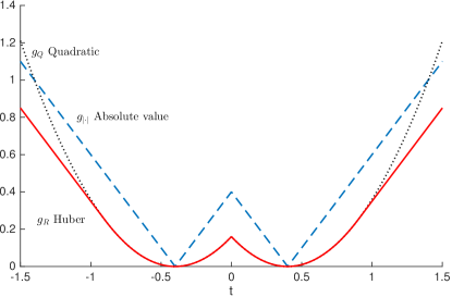
Figure 1 depicts a one-dimensional example of these different costs. We can observe in this simple example the main properties of the different cost functions, in terms of adaptation to low/medium-power Gaussian noise and high-power outlier spikes. Using (1) we can write our robust optimization problem as
| (2) |
where
| (3) |
This function is nonconvex and, in general, difficult to minimize. We shall provide a convex underestimator that tightly bounds each term of (3), thus leading to better estimation results than other relaxations which are not tight [17].
III Convex underestimator
To convexify we can replace each term by its convex hull111The convex hull of a function , i.e., its best possible convex underestimator, is defined as . It is hard to determine in general [18].,
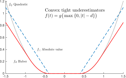
as depicted in Figure 2. Here, we observe that the high-power behavior is maintained, whereas the medium/low-power is only altered in the convexified area. We define the convex costs by composing any of the convex functions with a nondecreasing function
which, in turn, operates on the discrepancies
As and are nondecreasing and each one of the functions is convex, then
| (4) | ||||
is also convex. The cost function (4) also appears in Yousefi et al. [15] via a distinct reasoning. But the striking difference with respect to Yousefi et al. is how the cost (4) is exploited here to generate distributed solution methods where all nodes work in parallel, for the synchronous algorithm, or are randomly awaken, for the asynchronous algorithm.
III-A Approximation quality of the convex underestimator
The quality of the convexified quadratic problem was addressed in [5], which we summarize here for the reader’s convenience and extend to the two other convex problems.
The optimal value of the nonconvex , denoted by , is bounded by
where is the minimizer of the convex underestimator , and
is the minimum of function . A bound for the optimality gap is, thus,
It is evident that in all cases (quadratic, Huber, and absolute value) is equal to when and . When the function terms differ, say, for all edges222The same reasoning would apply to anchor terms. , we have , leading to
| (5) | |||||
| (6) | |||||
| (7) |
where
These bounds are an optimality gap guarantee available after the convexified problem is solved; they tell us how low our estimates can bring the original cost. Our bounds are tighter than the ones available a priori from applying [19, Th. 1], which are
| (8) | |||||
| (9) | |||||
| (10) |
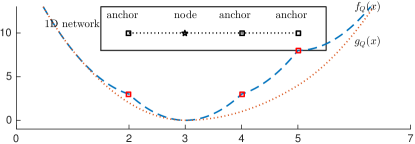
For a single-node 1D example whose costs for a single noise realization are exemplified in Figure 3,


| Cost | Eqs. (5)-(7) | Eqs. (8)-(10) | |
|---|---|---|---|
| Quadratic | 3.7019 | 5.5250 | 11.3405 |
| Absolute value | 1.1416 | 1.1533 | 3.0511 |
| Robust Huber | 0.1784 | 0.1822 | 0.4786 |
averaged over 500 Monte Carlo trials, are presented in Table I. The true average gap is also listed. In the Monte Carlo trials we sampled a set of zero mean Gaussian random variables with for the baseline Gaussian noise and obtained a noisy range measurement as in (27) below. One of the measurements is then corrupted by a zero mean random variable with , modelling outlier noise. These results show the tightness of the convexified function under such noisy conditions and also demonstrate the looseness of the a priori bounds in (8)-(10). We can observe in Figure 3 why the Huber-based relaxation will perform better than the other two: not only do we use a robust dissimilarity, but we also add a smaller optimality gap with the surrogate. In the end, the Huber-based approximation will be tighter, thus conferring robustness to the estimator, as pointed out by Destino and Abreu [4].
IV Distributed and robust sensor network localization
We construct our algorithm by rewriting (4) as the infimum of a sum of Huber functions composed with a norm, and then by rewriting each of the terms with an alternative representation that uncovers the possibility of a naturally distributed, optimal method for the estimation of the unknown sensor positions. For the first step, we state the following:
Proposition 1.
Each term of the first summation of (4), corresponding to the edge , has a variational representation
| (11) |
where is an optimization variable.
The proof is detailed in Appendix A.
IV-A Alternative representation of the Huber function composed with a norm
Using the variational representation from Proposition 1, we can rewrite the convex unconstrained minimization Problem (4) as the constrained problem
| (12) | ||||
where , , and . We put forward a new representation of the Huber function in (1), when composed with the norm of a vector as
| (13) |
where we denote by the squared distance of vector to a ball of radius centered at the origin. We use this representation to rewrite the cost in problem (12) as
and we further work the problem, leading to
where is the Cartesian product of the balls , is the Cartesian product of the balls , and is the squared distance to set (similarly for ). Matrix is the Kronecker product of the arc-node incidence matrix333The arc-node incidence matrix is a matrix. The rows and the columns of are indexed by and , respectively. The -entry of is 0 if node and edge are not incident, and otherwise it is 1 or -1 according to the direction agreed on the operation onset by the two nodes involved in edge . associated with the graph , and the identity matrix with dimension of the ambient space (usually, 2 or 3). The terms are the collections of the positions of the anchors within range of each node, and are the collections of associated variables. Consider the aggregation of variables ; we define the constraint set in (12) as
| (14) |
and the cost as
| (15) |
where , matrix , and is a selector matrix of the anchor terms associated with each separate node. With this notation, (12) becomes
| (16) | ||||
IV-B Gradient
To compute the gradient of the cost in (15), we need the gradient of the squared distance to a convex set — a result from convex analysis (see [18, Prop. X.3.2.2, Th. X.3.2.3]). Let us denote the squared distance to the convex set as
Then, from convex analysis, we know that is convex, differentiable, and its gradient is
| (17) |
where is the orthogonal projection of point onto the set ,
Knowing this, we can compute the gradient of (13) as
and the gradient of (15) as
| (18) | |||||
IV-C Lipschitz constant
It is widely known that projections onto convex sets shrink distances [20], i.e.,
and this means that the gradient of (13) is Lipschitz continuous with Lipschitz constant . Using this, we can compute a Lipschitz constant for (18). First, let us focus on the inter-node term in (18):
The maximum eigenvalue of can be bounded by
| (19) | |||||
where is the graph Laplacian, and is the maximum node degree of the network. A proof of the inequality is in Bapat [21]. In the same way, for the node-anchor terms, we have
and this constant can be upper-bounded by
| (20) | |||||
From (19) and (20) we can see that a Lipschitz constant for (15) is
| (21) |
We stress that this constant is small, does not depend on the size of the network, and can be computed in a distributed way [22].
IV-D Synchronous algorithm
The gradient in (18) and its Lipschitz continuity, with the constant in (21), equip us to use the optimal gradient optimization method due to Nesterov ([23][24]), further developed by Beck and Teboulle [25]. Firstly, we must write the problem as an unconstrained minimization using an indicator function , and incorporate the constraints in the problem formulation. Then we perform the proximal minimization of the unconstrained problem. The result for our reformulation is shown in Algorithm 1.
Here, and are the sets , and , respectively. Also, and are the constraint sets associated with the acquired measurements between sensors, and between anchors and sensors, respectively, and is the set of neighbor nodes of node . We denote the entries of regarding variable as . We observe that each block of at iteration will only need local neighborhood information, as shown in Algorithm 1. To demonstrate the natural distribution of the method we go back to (18). Here, the term only involves anchor measurements relative to each node, and so it is distributed. The term is less clear. The vector collects for all edges and to it we apply the projection operator onto the Cartesian product of balls. This is the same as applying a projection of each edge onto each ball. When left multiplying with we get . The left multiplication by will group at the position of each node variable the contributions of all incident edges to node . To update the variables we could designate one of the incident nodes as responsible for the update and then communicate the result to the non-computing neighbor. But, to avoid this expensive extra communication, we decide that each node should compute its own , where for all edges. Also, with this device, the gradient entry regarding variable would be . The symbol denotes the arc-node incidence matrix entry relative to edge (row index) and node (column index). As the projection onto a ball of radius centered at the origin can be written as then , and, thus, the gradient entry regarding variable becomes , as stated in Algorithm 1. Each node will update the current estimate of its own position, each one of the for all the incident edges and the anchor terms , if any. In step 6 we have the extrapolation step for each , whereas in steps 9 and 13 we can see the update of the extrapolation steps for each one of the edge variables , and , respectively.
IV-E Asynchronous algorithm
In Section IV-D we presented a distributed method addressing the robust network localization problem in a scalable manner, where each node uses information from its neighborhood and performs a set of simple arithmetic computations. But the results still depend critically on synchronous computation, where nodes progress in lockstep through iterations. As the number of processing nodes becomes very large, this synchronization can become seriously difficult — and unproductive. An asynchronous approach is called for in such very large-scale and faulty settings. In an asynchronous time model, the nodes move forward independently and algorithms withstand certain types of faults, like temporary unavailability of a node. To address this issue, we present a fully asynchronous method, based on a broadcast gossip scheme (c.f. Shah [26] for an extended survey of gossip algorithms).
Nodes are equipped with independent clocks ticking at random times (say, as Poisson point processes). When node ’s clock ticks, it performs the update of its variables and broadcasts the update to its neighbors. Let the order of node activation be collected in , a sequence of independent random variables taking values on the set , such that
| (22) |
Then, the asynchronous update of variables on node can be described as in Algorithm 2.
To compute the minimizer in step 6 of Algorithm 2 it is useful to recast Problem (16) as
| (23) | ||||
where the factor accounts for the duplicate terms when considering summations over nodes instead of over edges. By fixing the neighbor positions, each node solves a single source localization problem; this setup leads to
| (24) | ||||
where
| (25) | |||
Problem (24) is convex, solvable at each node by a general purpose solver. Nevertheless, that approach would not take advantage of the specific problem structure, thus depriving the solution of an efficient and simpler computational procedure. Again, Problem (24) can be solved by the Nesterov optimal first order method, because the gradient of is Lipschitz continuous in , and , accepting the same Lipschitz constant as , in (21).
V Convergence analysis
In this section we address the convergence of Algorithms 1 and 2. We provide convergence guarantees and rate of convergence for the synchronous version, and we also prove convergence for the asynchronous method.
V-A Synchronous algorithm
As shown in Section IV, Problem (16) is convex and the cost function has a Lipschitz continuous gradient. As proven by Nesterov ([23, 24]), and further developed by Beck and Teboulle [25], Algorithm 1 converges at the optimal rate ; specifically, , where is the optimal value and is a minimizer of Problem (16).
V-B Asynchronous algorithm
To investigate the convergence of Algorithm 2, we need the following assumptions:
Assumption 2.
The topology of the network conforms to:
-
•
The graph is connected;
-
•
There is at least one node in with an anchor measurement.
These assumptions are naturally fulfilled in the network localization problem: if the network is supporting several disconnected components, then each can be treated as a different network, and, for disambiguation, localization requires the availability of 3 anchors in 2D and 4 anchors in 3D.
The convergence of Algorithm 2 is stated next.
Theorem 3 (Almost sure convergence).
The reader can find the proof in Appendix B. It is also possible to state that, with probability one, Algorithm 2 converges in a finite number of iterations. The result is stated in the following theorem, also proven in Appendix B.
Theorem 4.
For a prescribed precision , the sequence of iterates converges in iterations. The expected value of this number of iterations is
| (26) |
where is a constant that depends on the specified .
VI Numerical experiments
VI-A Underestimator performance
We assess the performance of the three considered loss functions through simulation. The experimental setup consists in a uniquely localizable geometric network deployed in a square area with side of Km, with four anchors (blue squares in Figure 4) located at the corners, and ten sensors, (red stars). Measurements are also visible as dotted green lines. The average node degree444To characterize the network we use the concepts of node degree , which is the number of edges connected to node , and average node degree . of the network is . The regular noisy range measurements are generated according to
| (27) |
where is the true position of node , and are independent Gaussian random variables with zero mean and standard deviation , corresponding to an uncertainty of about m. Node is malfunctioning and all measurements related to it are corrupted by Gaussian noise with standard deviation , corresponding to an uncertainty of Km. The convex optimization problems were solved with cvx [27]. We ran Monte Carlo trials, sampling both regular and outlier noise.
The performance metric used to assess accuracy is the positioning error per sensor defined as
| (28) |
where corresponds to the position estimates for all sensors in Monte Carlo trial . The empirical mean of the positioning error is defined as
| (29) |
where is the number of Monte Carlo trials.
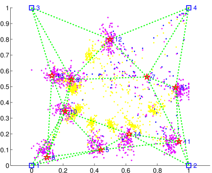
In Figure 4 we can observe that clouds of estimates from and gather around the true positions, except for the malfunctioning node . Note the increased spread of blue dots around nodes with edges connecting to node , indicating that better preserves the nodes’ ability to localize themselves, despite their confusing neighbor, node .
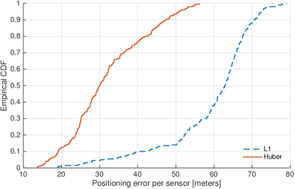
This intuition is confirmed by the empirical CDFs of estimation errors shown in Figure 5, which demonstrate that the Huber robust cost can reduce the error per sensor by an average of meters, when compared with the discrepancy. Also, as expected, the malfunctioning node cannot be positioned by any of the algorithms.
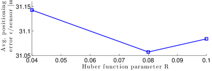
The sensitivity to the value of the Huber parameter in (1) is only moderate, as shown in Figure 6. In fact, the error per sensor of the proposed estimator is always the smallest for all tested values of the parameter. We observe that the error increases when approaches the standard deviation of the regular Gaussian noise, meaning that the Huber loss gets closer to the loss and, thus, is no longer adapted to the regular noise ( corresponds exactly to the loss); in the same way, as increases, so does the quadratic section, and the estimator gets less robust to outliers, so, again, the error increases.
Another interesting experiment is to see what happens when the faulty sensor produces measurements with consistent errors or bias. We ran Monte Carlo trials in the same setting, but node measurements are now consistently of the real distance to each neighbor.
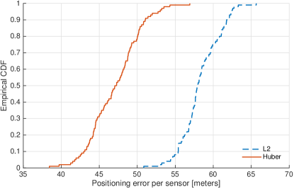
The empirical CDF for the positioning error per sensor is shown in Figure 7. Here we observe a significant performance gap between the alternative costs — in average about meters — so the Huber formulation proves to be superior even with biased sensors.
VI-B Performance of the distributed synchronous Algorithm 1
We tested Algorithm 1 using the same setup as in the previous section, with node contaminated with added Gaussian noise with standard deviation of .
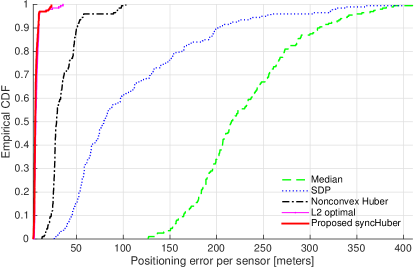
We benchmark our method comparing with the performance of the centralized solutions in Oğuz-Ekim et al., [1], which we denote as “Median” below, the SDP presented by Simonetto and Leus555In [17], the authors present a distributed ESDP algorithm which is a relaxation of the centralized SDP. As the simulation time for the distributed, edge-based algorithm is considerable we benchmarked against the tighter and more accurate centralized SDP solution. [17], and also the distributed locally convergent algorithm by Korkmaz and Van der Veen666This distributed method attacks directly the nonconvex cost (3), thus delivering a local solution, that depends on the initialization point. The algorithm was initialized with Gaussian noise. [13]. The results are summarized in Figure 8. Here the empirical CDFs of the positioning error (28) show a superior accuracy of our syncHuber algorithm.
When analyzing the results for the biased experiment as described in the previous section, it is noticeable that the syncHuber algorithm beats the state-of-the-art [5] for the quadratic discrepancy by more than 5 meters per sensor in average positioning error, as depicted in Figure 9.
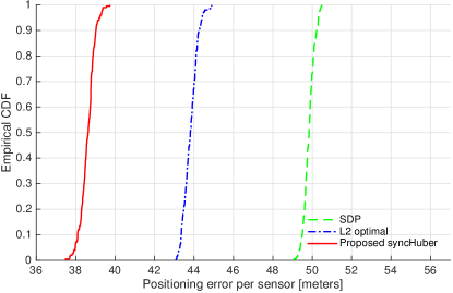
As expected from the results in the previous section, when we compare to a -type algorithm — in this case the “Median” from Oğuz-Ekim et al. [1] —
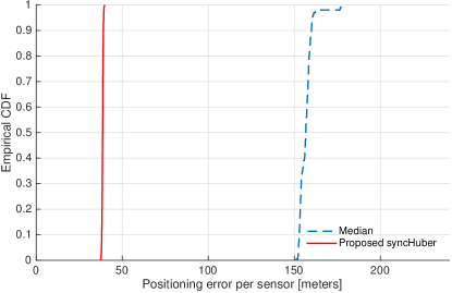
the improvement of performance of our solution is outstanding (on average about 120 metrs per sensor), as depicted in Figure 10.
VI-C Performance of the distributed asynchronous Algorithm 2
Here, we tested Algorithm 2, asyncHuber, using the same setup as in the previous sections, with node contaminated with added Gaussian noise with standard deviation of . We benchmarked it against the synchronous Algorithm 1, syncHuber, since both minimize the same cost function. The algorithms were allowed to run with the same communication load.
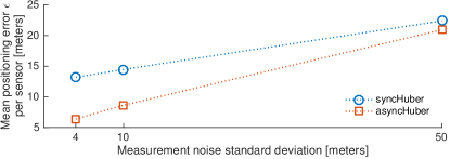
The mean positioning error for the considered noise levels is depicted in Figure 11. We can observe that the asyncHuber algorithm fares better than syncHuber for the same communication amount. This is an interesting phenomenon empirically observed in different optimization algorithms when comparing deterministic and randomized versions. In fact, Bertsekas and Tsitsiklis [28, Section 6.3.5] provide a proof of this behavior for a restricted class of algorithms.
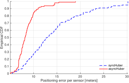
Figure 12 further explores the experimental data, by examining the CDF of the positioning error for the tested Monte Carlo trials. Here we see the superior accuracy of the asynchronous Huber Algorithm 2, for the same communications volume. We must, nevertheless, emphasize that this result does not correspond to a faster algorithm, in terms of running time: syncHuber in one iteration updates all of the nodes positions in parallel, and broadcasts the current estimates across neighbors, whereas in asyncHuber only one node operates at a time. As the wireless medium might be much more intensively used for synchronous updates than for random gossip interactions, it seems entirely possible that for the same operation time syncHuber will outperform asyncHuber — at the expense of greater overall power consumption.
VII Discussion and conclusions
We presented two distributed, fast, and robust localization algorithms that take noisy ranges and a few anchor locations, and output accurate estimates of the node positions. We approximated the difficult, nonconvex problem based on the Huber discrepancy in (2) with a convex envelope of terms, robust to outliers. How does the Huber-based approximation in (4) compares with similar and underestimators, frequent in robust estimation contexts? A smaller optimality gap means a more robust approximation [4]: We designed a bound that certifies the gap between the nonconvex and surrogate optimal values for Huber, and and shows a tighter gap in the Huber case. A numerical analysis of a star network in 1D unveiled that the optimality gap for the Huber approximation was one order of magnitude less than the quadratic or absolute value convexified problems, with respect to their nonconvex counterparts. Numerical network localization trials verify the surrogate robust behavior under different types of outlier noise. In order to develop a distributed method we needed to transform our cost. So, we proposed a new representation of the Huber function composed with a norm, and arrived at a novel distributed gradient method, syncHuber, with optimal convergence rate. But our syncHuber algorithm requires synchronization, which is a difficult demand for many applications. Thus, we put forward a novel asynchronous method for robust network localization, asyncHuber, converging with probability one. Nevertheless, like any other relaxation method, ours are prone to the anchor convex hull problem: preliminary results show the positioning accuracy degrades — albeit graciously — when nodes’ positions depart from the anchor convex hull. Arguably, this is not a big issue because engineers in general can control the choice or placement of anchoring landmarks, and can delimit the area under survey.
In sum, both our algorithms work with simple computations at each node and minimal communication payloads, have provable convergence and show a superior performance in our numerical experiments. Also, they do not require knowledge of a Hamiltonian path in the network, which simplifies real-world implementation, unlike the method presented by Yousefi et al. [15]. In average, the positioning error of Algorithm 1 is less 120m for a deployment in a square of 1Km sides than the state-of-the-art centralized method for robust network localization of Oğuz-Ekim et al. [1].
Acknowledgment
The authors would like to thank Pinar Oğuz-Ekim and Andrea Simonetto for providing the MATLAB implementations of their published algorithms. Also, we thank João Xavier for the interesting discussions during this research.
Appendix A Proof of Proposition 1
We define a function , and restate a generic term of the first summation in (4)
as
which represents the same mathematical object, because is always nonnegative. Now, we prove the equivalence relation (11), beginning by
| (30) |
We choose any , and note that
As is nondecreasing,
for all , and in particular,
which proves (30). We now establish
| (31) |
We choose , a minimizer of the optimization problem in the RHS of (31). We know that
and so
and as is monotonic,
for all . In particular,
which proves (31), and concludes the proof of Proposition 1.
Appendix B Proofs of Theorems 3 and 4
B-A Definitions
First, we review the definition of a block optimal point and describe some useful mathematical objects used on the proofs.
We define the sets
| (32) | |||||
| (33) | |||||
| (34) | |||||
| (35) | |||||
| (36) |
where is the set of all points whose distance to the optimal set is larger than , but also belong to the sublevel set of . We will see that the iterates of Algorithm 2 will belong to until they reach the absorbing set . We also define the expected improvement function as
| (37) |
and the coordinate optimal function as
| (38) |
It is easy to see that the expected improvement can also be written as
| (39) |
where is the probability of the event “node is awaken at time ” (we recall the independence of the random variables defined in (22)). For notational convenience, we introduce the function
| (40) |
which, by construction of Algorithm 2, is always non-negative.
B-A1 Auxiliary Lemmas
The analysis is founded in Lemma 7, where the symmetric of the expected improvement is said to attain a positive infimum on the set . Lemma 6 will be instrumental in the proof of Lemma 7 but contains also some useful properties of function and the solution set .
Lemma 6 (Basic properties).
Let as defined in (15). Then the following properties hold.
-
1.
is coercive;
-
2.
and ;
-
3.
is compact;
-
4.
If is block optimal for in , then it is global optimal for in .
Proof.
-
1.
By Assumption 2 there is a path from each node to some node which is connected to an anchor . Also, we know that, by definition, and are bounded by the ranges and . So these components of will have no effect in the limiting behavior of . If there are two cases: (1) there is at least one edge along the path from to where and , and so ; (2) if for all in the path between and , in particular we have and so , and in both cases , thus, is coercive.
-
2.
Function defined in (15) is a continuous, convex and real valued function lower bounded by zero; so, the infimum exists and is non-negative. To prove this infimum is attained and , we observe that the set is a cartesian product of the closed sets , and , and so is also closed. Now consider the set ; is a sublevel set of a continuous, coercive function and, thus, it is compact. For some , the intersection of and is nonempty and it is known that the intersection of a closed and a compact set is compact [30, Corollary to 2.35], so is compact. As function is convex, it is also continuous on the compact set , and by the extreme value theorem, the value is attained and it is obvious that .
-
3.
for , and we deduced in the previous proof that is compact.
-
4.
If is block-optimal, then for all and for all . When stacking the inequalities for all , we get , which proves the claim.∎
Lemma 7.
Proof.
We start by proving the first claim, for all . Suppose ; then, by Equation (39)
which means is block optimal; by Lemma 6, is, then, global optimal, which contradicts the fact that belongs to the set . The second claim follows by observing that is a sum of real valued functions and, thus, a real valued function, and that is bounded below by zero in and so it has a positive infimum for . ∎
B-A2 Theorems
Equipped with the previous Lemmas, we are now ready to prove the Theorems stated in Section V-B.
Proof of Theorem 3.
We denote the random variable corresponding to the outcome of the -th loop step of Algorithm 2 as . The expected value of the expected improvement function is
where the second equality comes from the tower property documented, e.g., in Williams [31]. This expectation can also be written as
By combining both we get
which can be further bounded using Lemma 7 as
where . By expanding the recursion we obtain
which provides a bound on the sum of probabilities when rearranged as
Taking up to infinity, we obtain
This means the infinite series of probabilities assumes a finite value; by the Borel-Cantelli Lemma, we get
where stands for infinitely often. This concludes the proof, since this statement is equivalent to the first claim of Theorem 3. ∎
Proof of Theorem 4.
Consider redefining the sets in (33) and (34) as
thus leading to
Using the same arguments as in Lemma 7, we can prove that
We now define a sequence of points such that
and the sequence of real values
The expected value of is
Summing these expectations over time, we get
Taking to infinity and interchanging integration and summation we obtain
From the definition of we can write
thus obtaining the result
which is a finite number. This completes the proof. ∎
References
- [1] P. Oğuz-Ekim, J. Gomes, J. Xavier, and P. Oliveira, “Robust localization of nodes and time-recursive tracking in sensor networks using noisy range measurements,” Signal Processing, IEEE Transactions on, vol. 59, no. 8, pp. 3930 –3942, Aug. 2011.
- [2] P. Biswas, T.-C. Liang, K.-C. Toh, Y. Ye, and T.-C. Wang, “Semidefinite programming approaches for sensor network localization with noisy distance measurements,” Automation Science and Engineering, IEEE Transactions on, vol. 3, no. 4, pp. 360 –371, Oct. 2006.
- [3] Y. Shang, W. Rumi, Y. Zhang, and M. Fromherz, “Localization from connectivity in sensor networks,” Parallel and Distributed Systems, IEEE Transactions on, vol. 15, no. 11, pp. 961 – 974, Nov. 2004.
- [4] G. Destino and G. Abreu, “On the maximum likelihood approach for source and network localization,” Signal Processing, IEEE Transactions on, vol. 59, no. 10, pp. 4954 –4970, Oct. 2011.
- [5] C. Soares, J. Xavier, and J. Gomes, “Simple and fast convex relaxation method for cooperative localization in sensor networks using range measurements,” Signal Processing, IEEE Transactions on, vol. 63, no. 17, pp. 4532–4543, Sept 2015.
- [6] J. Costa, N. Patwari, and A. Hero III, “Distributed weighted-multidimensional scaling for node localization in sensor networks,” ACM Transactions on Sensor Networks (TOSN), vol. 2, no. 1, pp. 39–64, 2006.
- [7] G. Calafiore, L. Carlone, and M. Wei, “Distributed optimization techniques for range localization in networked systems,” in Decision and Control (CDC), 2010 49th IEEE Conference on, Dec. 2010, pp. 2221–2226.
- [8] C. Soares, J. Xavier, and J. Gomes, “Distributed, simple and stable network localization,” in Signal and Information Processing (GlobalSIP), 2014 IEEE Global Conference on, Dec 2014, pp. 764–768.
- [9] A. Ihler, I. Fisher, J.W., R. Moses, and A. Willsky, “Nonparametric belief propagation for self-localization of sensor networks,” Selected Areas in Communications, IEEE Journal on, vol. 23, no. 4, pp. 809 – 819, Apr. 2005.
- [10] J. Ash and R. Moses, “Outlier compensation in sensor network self-localization via the EM algorithm,” in Acoustics, Speech, and Signal Processing, 2005. Proceedings. (ICASSP ’05). IEEE International Conference on, vol. 4, March 2005, pp. iv/749–iv/752 Vol. 4.
- [11] F. Yin, A. Zoubir, C. Fritsche, and F. Gustafsson, “Robust cooperative sensor network localization via the EM criterion in LOS/NLOS environments,” in Signal Processing Advances in Wireless Communications (SPAWC), 2013 IEEE 14th Workshop on, June 2013, pp. 505–509.
- [12] P. Forero and G. Giannakis, “Sparsity-exploiting robust multidimensional scaling,” Signal Processing, IEEE Transactions on, vol. 60, no. 8, pp. 4118 –4134, Aug. 2012.
- [13] S. Korkmaz and A.-J. van der Veen, “Robust localization in sensor networks with iterative majorization techniques,” in Acoustics, Speech and Signal Processing, 2009. ICASSP 2009. IEEE International Conference on, Apr. 2009, pp. 2049 –2052.
- [14] P. J. Huber, “Robust estimation of a location parameter,” The Annals of Mathematical Statistics, vol. 35, no. 1, pp. 73–101, 1964.
- [15] S. Yousefi, X. W. Chang, and B. Champagne, “Distributed cooperative localization in wireless sensor networks without NLOS identification,” in Positioning, Navigation and Communication (WPNC), 2014 11th Workshop on, March 2014, pp. 1–6.
- [16] D. Blatt and A. Hero, “Energy-based sensor network source localization via projection onto convex sets,” Signal Processing, IEEE Transactions on, vol. 54, no. 9, pp. 3614–3619, Sept. 2006.
- [17] A. Simonetto and G. Leus, “Distributed maximum likelihood sensor network localization,” Signal Processing, IEEE Transactions on, vol. 62, no. 6, pp. 1424–1437, Mar. 2014.
- [18] J.-B. Hiriart-Urruty and C. Lemaréchal, Convex analysis and minimization algorithms. Springer-Verlag Limited, 1993.
- [19] M. Udell and S. Boyd, “Bounding duality gap for problems with separable objective,” Computational Optimization and Applications, vol. 64, no. 2, pp. 355–378, 2016.
- [20] R. Phelps, “Convex sets and nearest points,” Proceedings of the American Mathematical Society, vol. 8, no. 4, pp. 790–797, 1957.
- [21] R. B. Bapat, Graphs and matrices. Springer, 2010.
- [22] F. R. Chung, Spectral graph theory. American Mathematical Soc., 1997, vol. 92.
- [23] Y. Nesterov, “A method of solving a convex programming problem with convergence rate ,” in Soviet Mathematics Doklady, vol. 27, no. 2, 1983, pp. 372–376.
- [24] ——, Introductory Lectures on Convex Optimization: A Basic Course. Kluwer Academic Publishers, 2004.
- [25] A. Beck and M. Teboulle, “A fast iterative shrinkage-thresholding algorithm for linear inverse problems,” SIAM journal on imaging sciences, vol. 2, no. 1, pp. 183–202, 2009.
- [26] D. Shah, Gossip algorithms. Now Publishers Inc, 2009.
- [27] M. Grant and S. Boyd, “CVX: Matlab software for disciplined convex programming, version 1.21,” http://cvxr.com/cvx, Apr. 2011.
- [28] D. P. Bertsekas and J. N. Tsitsiklis, Parallel and distributed computation: numerical methods. Upper Saddle River, NJ, USA: Prentice-Hall, Inc., 1989.
- [29] D. Jakovetic, J. Xavier, and J. Moura, “Cooperative convex optimization in networked systems: Augmented lagrangian algorithms with directed gossip communication,” Signal Processing, IEEE Transactions on, vol. 59, no. 8, pp. 3889–3902, Aug. 2011.
- [30] W. Rudin, Principles of Mathematical Analysis, ser. International series in pure and applied mathematics. McGraw-Hill, 1976.
- [31] D. Williams, Probability with martingales. Cambridge university press, 1991.