Analyzing the cosmic variance limit of remote dipole measurements of the cosmic microwave background using the large-scale kinetic Sunyaev Zel’dovich effect

Alexandra Terrana    Mary-Jean Harris    Matthew C. Johnson
Abstract

Due to cosmic variance we cannot learn any more about large-scale inhomogeneities from the primary cosmic microwave background (CMB) alone. More information on large scales is essential for resolving large angular scale anomalies in the CMB. Here we consider cross correlating the large-scale kinetic Sunyaev Zel’dovich (kSZ) effect and probes of large-scale structure, a technique known as kSZ tomography. The statistically anisotropic component of the cross correlation encodes the CMB dipole as seen by free electrons throughout the observable Universe, providing information about long wavelength inhomogeneities. We compute the large angular scale power asymmetry, constructing the appropriate transfer functions, and estimate the cosmic variance limited signal to noise for a variety of redshift bin configurations. The signal to noise is significant over a large range of power multipoles and numbers of bins. We present a simple mode counting argument indicating that kSZ tomography can be used to estimate more modes than the primary CMB on comparable scales. A basic forecast indicates that a first detection could be made with next-generation CMB experiments and galaxy surveys. This paper motivates a more systematic investigation of how close to the cosmic variance limit it will be possible to get with future observations.

1 Introduction

The cosmic microwave background (CMB) has been an extraordinarily powerful tool for precision cosmology, establishing the standard model, ΛΛ\LambdaCDM, at high confidence. However, on very large-scales, CMB measurements are limited by cosmic variance, implying that we can not hope to learn any more about large scale inhomogeneities from the primary CMB alone. Given that nearly all of the hints we have of departures from ΛΛ\LambdaCDM are on the very largest scales (for a recent summary of CMB anomalies see [1]), there is strong motivation to go beyond the primary CMB to learn more. Constraints from probes of Large Scale Structure (LSS), such as next-generation galaxy surveys (e.g [2]) and 21cm measurements (e.g. [3, 4]), are poised to become increasingly important for many cosmological parameters. Even still, when it comes to measuring inhomogeneities on scales Gpcgreater-than-or-equivalent-toabsentGpc\gtrsim{\rm Gpc}, there will be limited additional constraining power in all but the most ambitious scenarios (e.g. 21cm dark ages cosmology [5]). In this paper, we investigate the viability of an additional probe of large scale inhomogeneities: large scale kinetic Sunyaev Zel’dovich (kSZ) tomography.

The kSZ effect is a CMB temperature anisotropy arising from the Compton scattering of CMB photons by the bulk motion of free electrons with respect to the CMB rest frame [6]. There are two main contributions to the kSZ effect: the early-time kSZ effect which arises due to patchy reionization [7, 8, 9] (see e.g. [10] for a recent update), and the late-time kSZ effect arising from free electrons in large scale structure (e.g. galaxy clusters) and the intergalactic medium. Thus far, only the latter contribution has been detected. This was achieved by looking for the contribution to CMB temperature anisotropies induced by the pairwise motion of clusters [11, 12, 13, 14]; a (somewhat low significance) detection has also been made at the level of the temperature angular power spectrum [15]. Next-generation “Stage 3” and “Stage 4” CMB experiments [16, 17] will have the ability to make high-significance measurements of the kSZ effect.111It will at this point become important to separate the early-time and late-time kSZ effects to maximize the science return; for a proposal in this direction see Ref. [18]. Realizing the full potential of kSZ measurements will continue to rely heavily on cross correlations with future probes of LSS, making the dramatic improvements to come with the next generation of redshift surveys and 21cm measurements equally important. Such cross correlations also open the door to determining the contribution to the global kSZ signal from different redshifts, a technique known as kSZ tomography [19, 20, 21, 22, 23, 24, 25, 26].

The science case for precision measurements of the kSZ effect is quite broad. In addition to revolutionizing our understanding of reionization, it has the power to probe missing baryons e.g. [19, 27, 28], make precision tests of gravity [29, 30, 31], probe anomalous bulk flows [32, 33, 34, 35, 36, 37, 38], constrain the properties of dark energy and dark matter [39, 40], constrain the masses of neutrinos [41], test the Copernican principle [42, 21, 43], constrain the present day vacuum decay rate [44], and test the hypothesis that we inhabit an eternally inflating multiverse [45].

The contribution to the kSZ effect from each free electron is proportional to the locally observed CMB dipole, and because each free electron probes a different portion of the surface of last scattering, measurements of the kSZ effect can in principle yield information about the homogeneity of the Universe. This is why measurements of the kSZ effect can be so constraining for scenarios that predict a deviation from large-scale homogeneity, such as many of those listed above. Note that this is a dramatically different regime than the one typically explored, for example in the pairwise motion of clusters that yielded the first detection. This large-scale kSZ effect is sensitive to the Sachs Wolfe and integrated Sachs Wolfe components of the dipole, in addition to the Doppler component from peculiar velocities, and can therefore in principle yield more large-scale information than peculiar velocity surveys or direct measurements of the density field through various tracers of LSS. As mentioned above, cross correlation with tracers of LSS, and therefore kSZ tomography, is key to extracting the most information possible. As we show in more detail below, information about large scale homogeneity is encoded in a statistical anisotropy of the direct correlation of tracers of large scale structure and the small angular scale CMB, e.g. a power asymmetry. Importantly, the contribution to this signal from small-scale peculiar velocities vanishes [20].

The power of kSZ tomography to probe the large scale homogeneity of the Universe has been highlighted previously, notably in refs. [33, 21, 44, 45].222The polarized component of the late-time kSZ effect also has the potential to constrain homogeneity on large scales [46, 47, 48, 49, 50, 51, 52], but we do not consider it further here. These papers considered theoretical extensions to ΛΛ\LambdaCDM where a signal could hopefully be detected with current and near-future experiments. However, as the sensitivity and resolution of CMB experiments continues to develop and as our ability to probe LSS improves, we might hope to enter an era where large scale kSZ tomography becomes a tool not just for constraining exotic scenarios, but for measuring the inhomogeneities we know to exist: those responsible for the large scale temperature anisotropies in the primary CMB.

The goal of this paper is to explore this eventuality in the most optimistic, cosmic variance limited, scenario. More specifically, we compute the angular spectrum of the asymmetry in the kSZ-LSS cross power expected in ΛΛ\LambdaCDM as a function of redshift. Comparing this signal to the accidental power asymmetry expected from the statistically isotropic components of the kSZ effect (the dominant source of CMB temperature anisotropies on small angular scales), we find that the signal-to-noise can be significant (S/N𝒪(102103)similar-to𝑆𝑁𝒪superscript102superscript103S/N\sim\mathcal{O}(10^{2}-10^{3})) over a wide range of angular scales (max𝒪(100)similar-tosubscriptmax𝒪100\ell_{\rm max}\sim\mathcal{O}(100)) and in a large number (Nbin𝒪(10100)similar-tosubscript𝑁bin𝒪10100N_{\rm bin}\sim\mathcal{O}(10-100)) of redshift bins. A simple mode counting argument indicates that there is in principle more information in the power asymmetry than in the primary CMB on the relevant scales, for a sufficient number of redshift bins (Nbin30greater-than-or-equivalent-tosubscript𝑁bin30N_{\rm bin}\gtrsim 30). We present a basic forecast, indicating that a first detection could be made with next-generation CMB experiments and galaxy surveys.

The plan of the paper is as follows. In section 2, the large-scale late-time kSZ effect is summarized along with a derivation of the large-scale effective velocity. Section 3 describes simulations of the large-scale effective velocity field. Section 4 outlines how kSZ tomography can be used to extract the large-scale effective velocity. Then, we derive the cosmic variance limited noise in section 5 and estimate the signal using both an RMS estimate and simulations in section 6. In section 7 we provide an estimate for the number of modes that can be obtained using cosmic variance limited kSZ tomography, showing that in principle more information can be extracted than is contained in the primary CMB on comparable scales. Finally, we assess the detectability of the signal with next-generation CMB experiments and galaxy surveys in section 8; we conclude in section 9. A number of results are collected in the Appendix.

2 The large-scale kSZ effect

The kinetic Sunyaev Zel’ dolvich effect arises from Compton scattering of CMB photons by free electrons moving with respect to the CMB rest frame. This produces temperature anisotropies given by an integral along the line of sight:

ΔTT|kSZ(𝐧^e)evaluated-atΔ𝑇𝑇kSZsubscript^𝐧𝑒\displaystyle\frac{\Delta T}{T}\bigg{|}_{\text{kSZ}}({\bf\hat{n}}_{e}) =σT0χre𝑑χeae(χe)ne(𝐧^e,χe)𝐯eff(𝐧^e,χe)𝐧^eabsentsubscript𝜎𝑇superscriptsubscript0subscript𝜒redifferential-dsubscript𝜒𝑒subscript𝑎𝑒subscript𝜒𝑒subscript𝑛𝑒subscript^𝐧𝑒subscript𝜒𝑒subscript𝐯effsubscript^𝐧𝑒subscript𝜒𝑒subscript^𝐧𝑒\displaystyle=-\sigma_{T}\int_{0}^{\chi_{\rm re}}d\chi_{e}\ a_{e}(\chi_{e})\ n_{e}({\bf\hat{n}}_{e},\chi_{e})\ {\bf v}_{\text{eff}}({\bf\hat{n}}_{e},\chi_{e})\cdot{\bf\hat{n}}_{e} (2.1)
=σT0χre𝑑χeae(χe)n¯e(χe)(1+δ(𝐧^e,χe))veff(𝐧^e,χe).absentsubscript𝜎𝑇superscriptsubscript0subscript𝜒redifferential-dsubscript𝜒𝑒subscript𝑎𝑒subscript𝜒𝑒subscript¯𝑛𝑒subscript𝜒𝑒1𝛿subscript^𝐧𝑒subscript𝜒𝑒subscript𝑣effsubscript^𝐧𝑒subscript𝜒𝑒\displaystyle=-\sigma_{T}\int_{0}^{\chi_{\rm re}}d\chi_{e}\ a_{e}(\chi_{e})\ \bar{n}_{e}(\chi_{e})\ (1+\delta({\bf\hat{n}}_{e},\chi_{e}))\ v_{\rm eff}({\bf\hat{n}}_{e},\chi_{e}). (2.2)

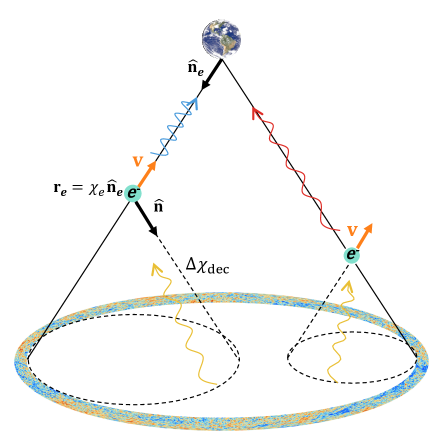
The geometry is depicted in figure 1. In eq. (2.1), σTsubscript𝜎𝑇\sigma_{T} is the Thomson cross-section, ne(𝐧^e,χe)subscript𝑛𝑒subscript^𝐧𝑒subscript𝜒𝑒n_{e}({\bf\hat{n}}_{e},\chi_{e}) is the electron number density, 𝐧^esubscript^𝐧𝑒{\bf\hat{n}}_{e} is the angular direction on the sky to the scatterer, and χesubscript𝜒𝑒\chi_{e} is the comoving radial coordinate to the scatterer along our past light cone,

χe=0zedzH(z)=1aedaH(a)a2,subscript𝜒𝑒superscriptsubscript0subscript𝑧𝑒𝑑𝑧𝐻𝑧superscriptsubscript1subscript𝑎𝑒𝑑𝑎𝐻𝑎superscript𝑎2\chi_{e}=\int_{0}^{z_{e}}\frac{dz}{H(z)}=-\int_{1}^{a_{e}}\ \frac{da}{H(a)a^{2}}, (2.3)

where zesubscript𝑧𝑒z_{e} and aesubscript𝑎𝑒a_{e} are the scatterer’s redshift and scale factor respectively. Below, we will use χesubscript𝜒𝑒\chi_{e} and zesubscript𝑧𝑒z_{e} interchangeably. In the second line of (2.2), we have written the electron number density as ne(𝐧^e,χe)=n¯e(χe)(1+δ(𝐧^e,χe))subscript𝑛𝑒subscript^𝐧𝑒subscript𝜒𝑒subscript¯𝑛𝑒subscript𝜒𝑒1𝛿subscript^𝐧𝑒subscript𝜒𝑒n_{e}({\bf\hat{n}}_{e},\chi_{e})=\bar{n}_{e}(\chi_{e})(1+\delta({\bf\hat{n}}_{e},\chi_{e})) in terms of the average electron number density n¯e(χe)subscript¯𝑛𝑒subscript𝜒𝑒\bar{n}_{e}(\chi_{e}), and the density perturbation δ𝛿\delta, and replaced 𝐯eff(𝐧^e,χe)𝐧^esubscript𝐯effsubscript^𝐧𝑒subscript𝜒𝑒subscript^𝐧𝑒{\bf v_{\text{eff}}}({\bf\hat{n}}_{e},\chi_{e})\cdot{\bf\hat{n}}_{e} with the projection along the line of sight veff(𝐧^e,χe)subscript𝑣effsubscript^𝐧𝑒subscript𝜒𝑒v_{\rm eff}({\bf\hat{n}}_{e},\chi_{e}).

Refer to caption
Figure 1: Scattering of CMB photons off free electrons on our past light cone. The position of an electron is described in terms of its direction 𝐧^esubscript^𝐧𝑒{\bf\hat{n}}_{e} and comoving distance χesubscript𝜒𝑒\chi_{e}. The direction from the electron to a point on the surface of last scattering is denoted by 𝐧^^𝐧{\bf\hat{n}} and the distance to last scattering by ΔχdecΔsubscript𝜒dec\Delta\chi_{\text{dec}}.

The quantity denoted by veff(𝐧^e,χe)subscript𝑣effsubscript^𝐧𝑒subscript𝜒𝑒v_{\rm eff}({\bf\hat{n}}_{e},\chi_{e}) is the CMB dipole observed by each electron, projected along the line of sight:

veff(𝐧^e,χe)=34πd2𝐧^Θ(𝐧^e,χe,𝐧^)(𝐧^𝐧^e),subscript𝑣effsubscript^𝐧𝑒subscript𝜒𝑒34𝜋superscript𝑑2^𝐧Θsubscript^𝐧𝑒subscript𝜒𝑒^𝐧^𝐧subscript^𝐧𝑒v_{\rm eff}({\bf\hat{n}}_{e},\chi_{e})=\frac{3}{4\pi}\int d^{2}{\bf\hat{n}}\ \Theta({\bf\hat{n}}_{e},\chi_{e},{\bf\hat{n}})\ ({\bf\hat{n}}\cdot{\bf\hat{n}}_{e}), (2.4)

where, for a freely falling electron at position 𝐫eχe𝐧^esubscript𝐫𝑒subscript𝜒𝑒subscript^𝐧𝑒{\bf r}_{e}\equiv\chi_{e}{\bf\hat{n}}_{e}, the CMB temperature it sees along the direction 𝐧^^𝐧{\bf\hat{n}} is given by

Θ(𝐧^e,χe,𝐧^)=ΘSW(𝐧^e,χe,𝐧^)+ΘDoppler(𝐧^e,χe,𝐧^)+ΘISW(𝐧^e,χe,𝐧^).Θsubscript^𝐧𝑒subscript𝜒𝑒^𝐧subscriptΘSWsubscript^𝐧𝑒subscript𝜒𝑒^𝐧subscriptΘDopplersubscript^𝐧𝑒subscript𝜒𝑒^𝐧subscriptΘISWsubscript^𝐧𝑒subscript𝜒𝑒^𝐧\Theta({\bf\hat{n}}_{e},\chi_{e},{\bf\hat{n}})=\Theta_{\rm SW}({\bf\hat{n}}_{e},\chi_{e},{\bf\hat{n}})+\Theta_{\rm Doppler}({\bf\hat{n}}_{e},\chi_{e},{\bf\hat{n}})+\Theta_{\rm ISW}({\bf\hat{n}}_{e},\chi_{e},{\bf\hat{n}}). (2.5)

The three contributions come from the Sachs-Wolfe (SW) effect generated by the gravitational potential on the LSS, the Doppler effect due to peculiar motion of photons on the LSS and peculiar motion of electrons at redshift zesubscript𝑧𝑒z_{e}, and the integrated Sachs-Wolfe (ISW) effect.

Working in Newtonian gauge

ds2=(1+2Ψ)dt2+a2(t)(12Ψ)d𝐱2,𝑑superscript𝑠212Ψ𝑑superscript𝑡2superscript𝑎2𝑡12Ψ𝑑superscript𝐱2ds^{2}=-(1+2\Psi)dt^{2}+a^{2}(t)(1-2\Psi)d{\bf x}^{2}, (2.6)

the Sachs-Wolfe contribution is given by

ΘSW(𝐧^e,χe,𝐧^)=(2DΨ(χdec)32)Ψi(𝐫dec),subscriptΘSWsubscript^𝐧𝑒subscript𝜒𝑒^𝐧2subscript𝐷Ψsubscript𝜒dec32subscriptΨ𝑖subscript𝐫dec\Theta_{\rm SW}({\bf\hat{n}}_{e},\chi_{e},{\bf\hat{n}})=\left(2D_{\Psi}(\chi_{\text{dec}})-\frac{3}{2}\right)\Psi_{i}({\bf r}_{\text{dec}}), (2.7)

where 𝐫decχe𝐧^e+Δχdec𝐧^subscript𝐫decsubscript𝜒𝑒subscript^𝐧𝑒Δsubscript𝜒dec^𝐧{\bf r}_{\rm dec}\equiv\chi_{e}{\bf\hat{n}}_{e}+\Delta\chi_{\text{dec}}{\bf\hat{n}} with Δχdec=Δχ(adec)=aeadec𝑑a(H(a)a2)1Δsubscript𝜒decΔ𝜒subscript𝑎decsuperscriptsubscriptsubscript𝑎𝑒subscript𝑎decdifferential-d𝑎superscript𝐻𝑎superscript𝑎21\Delta\chi_{\text{dec}}=\Delta\chi(a_{\rm dec})=-\int_{a_{e}}^{a_{\text{dec}}}da\left({H(a)a^{2}}\right)^{-1} the distance along the electron’s past light cone to decoupling. More generally, we will define

Δχ(a)=aeadaH(a)a2.Δ𝜒𝑎superscriptsubscriptsubscript𝑎𝑒𝑎𝑑𝑎𝐻𝑎superscript𝑎2\Delta\chi(a)=-\int_{a_{e}}^{a}\frac{da}{H(a)a^{2}}. (2.8)

In eq. (2.7) we have used the growth function, DΨ(a)subscript𝐷Ψ𝑎D_{\Psi}(a), which relates the potential to its primordial value at a0𝑎0a\rightarrow 0 through the definition Ψ(𝐫,a)=DΨ(a)Ψi(𝐫)Ψ𝐫𝑎subscript𝐷Ψ𝑎subscriptΨ𝑖𝐫\Psi({\bf r},a)=D_{\Psi}(a)\Psi_{i}({\bf r}). The growth function is well approximated on superhorizon scales by

DΨ(a)ΨSH(a)ΨSH,i=161+y+9y3+2y28y1610y3[52ΩmE(a)a0adaE3(a)a3],subscript𝐷Ψ𝑎subscriptΨSH𝑎subscriptΨSHi161𝑦9superscript𝑦32superscript𝑦28𝑦1610superscript𝑦3delimited-[]52subscriptΩ𝑚𝐸𝑎𝑎superscriptsubscript0𝑎𝑑𝑎superscript𝐸3𝑎superscript𝑎3D_{\Psi}(a)\equiv\frac{\Psi_{\rm SH}(a)}{\Psi_{\rm SH,i}}=\frac{16\sqrt{1+y}+9y^{3}+2y^{2}-8y-16}{10y^{3}}\left[\frac{5}{2}\Omega_{m}\frac{E(a)}{a}\int_{0}^{a}\frac{da}{E^{3}(a)\ a^{3}}\right], (2.9)

where E(a)=Ωma3+ΩΛ𝐸𝑎subscriptΩ𝑚superscript𝑎3subscriptΩΛE(a)=\sqrt{\Omega_{m}a^{-3}+\Omega_{\Lambda}} is the normalized Hubble parameter.

The Doppler component is given by

ΘDoppler(𝐧^e,χe,𝐧^)=𝐧^[𝐯(𝐫e,χe)𝐯(𝐫dec,χdec)].subscriptΘDopplersubscript^𝐧𝑒subscript𝜒𝑒^𝐧^𝐧delimited-[]𝐯subscript𝐫𝑒subscript𝜒𝑒𝐯subscript𝐫decsubscript𝜒dec\Theta_{\rm Doppler}({\bf\hat{n}}_{e},\chi_{e},{\bf\hat{n}})={\bf\hat{n}}\cdot[{\bf v}({\bf r}_{e},\chi_{e})-{\bf v}({\bf r}_{\rm dec},\chi_{\text{dec}})]. (2.10)

The velocities can be related to the potential through

𝐯=2a2c2H(a)H02Ωmy4+3y[Ψ+dΨdlna],𝐯2superscript𝑎2superscript𝑐2𝐻𝑎subscriptsuperscript𝐻20subscriptΩ𝑚𝑦43𝑦delimited-[]Ψ𝑑Ψ𝑑𝑎{\bf v}=-\frac{2a^{2}c^{2}H(a)}{H^{2}_{0}\Omega_{m}}\frac{y}{4+3y}\left[{\bf\nabla}\Psi+\frac{d{\bf\nabla}\Psi}{d\ln a}\right], (2.11)

which is valid on all scales. On large scales, we can use this expression to define a velocity growth function Dv(a)subscript𝐷𝑣𝑎D_{v}(a):

𝐯=2a2c2H(a)H02Ωmy4+3y[DΨ+dDΨdlna]Ψi,𝐯2superscript𝑎2superscript𝑐2𝐻𝑎subscriptsuperscript𝐻20subscriptΩ𝑚𝑦43𝑦delimited-[]subscript𝐷Ψ𝑑subscript𝐷Ψ𝑑𝑎subscriptΨ𝑖{\bf v}=-\frac{2a^{2}c^{2}H(a)}{H^{2}_{0}\Omega_{m}}\frac{y}{4+3y}\left[D_{\Psi}+\frac{dD_{\Psi}}{d\ln a}\right]{\bf\nabla}\Psi_{i}, (2.12)

where

Dv(a)2a2H(a)H02Ωmy4+3y[DΨ+dDΨdlna].subscript𝐷𝑣𝑎2superscript𝑎2𝐻𝑎subscriptsuperscript𝐻20subscriptΩ𝑚𝑦43𝑦delimited-[]subscript𝐷Ψ𝑑subscript𝐷Ψ𝑑𝑎D_{v}(a)\equiv\frac{2a^{2}H(a)}{H^{2}_{0}\Omega_{m}}\frac{y}{4+3y}\left[D_{\Psi}+\frac{dD_{\Psi}}{d\ln a}\right]. (2.13)

Finally, the ISW term is given by

ΘISW(𝐧^e,χe,𝐧^)=2adecaedΨda(𝐫(a),a)𝑑a=2adecaedDΨdaΨi(𝐫(a))𝑑a.subscriptΘISWsubscript^𝐧𝑒subscript𝜒𝑒^𝐧2superscriptsubscriptsubscript𝑎decsubscript𝑎𝑒𝑑Ψ𝑑𝑎𝐫𝑎𝑎differential-d𝑎2superscriptsubscriptsubscript𝑎decsubscript𝑎𝑒𝑑subscript𝐷Ψ𝑑𝑎subscriptΨ𝑖𝐫𝑎differential-d𝑎\Theta_{\rm ISW}({\bf\hat{n}}_{e},\chi_{e},{\bf\hat{n}})=2\int_{a_{\rm dec}}^{a_{e}}\frac{d\Psi}{da}({\bf r}(a),a)da=2\int_{a_{\rm dec}}^{a_{e}}\frac{dD_{\Psi}}{da}\Psi_{i}({\bf r}(a))da. (2.14)

Here, 𝐫(a)=𝐫e+Δχ(a)𝐧^𝐫𝑎subscript𝐫𝑒Δ𝜒𝑎^𝐧{\bf r}(a)={\bf r}_{e}+\Delta\chi(a)\ {\bf\hat{n}}.

2.1 Fourier kernel for the effective velocity

Relating each contribution to the effective velocity to the primordial potential ΨisubscriptΨ𝑖\Psi_{i} allows us to define a kernel in Fourier space relating ΨisubscriptΨ𝑖\Psi_{i} to the effective velocity. The details can be found in Appendix A, which results in the expression

veff(𝐧^e,χe)=id3k(2π)3T(k)Ψ~i(𝐤)𝒦v(k,χe)𝒫1(𝐤^𝐧^e)eiχe𝐤𝐧^e,subscript𝑣effsubscript^𝐧𝑒subscript𝜒𝑒𝑖superscript𝑑3𝑘superscript2𝜋3𝑇𝑘subscript~Ψ𝑖𝐤superscript𝒦𝑣𝑘subscript𝜒𝑒subscript𝒫1^𝐤subscript^𝐧𝑒superscript𝑒𝑖subscript𝜒𝑒𝐤subscript^𝐧𝑒v_{\rm eff}({\bf\hat{n}}_{e},\chi_{e})=i\int\frac{d^{3}k}{(2\pi)^{3}}\ T(k)\tilde{\Psi}_{i}({\bf k})\ \mathcal{K}^{v}(k,\chi_{e})\ \mathcal{P}_{1}({\bf\hat{k}}\cdot{\bf\hat{n}}_{e})\ e^{i\chi_{e}{\bf k}\cdot{\bf\hat{n}}_{e}}, (2.15)

where we have incorporated the transfer function T(k)𝑇𝑘T(k) for the potential to account for sub-horizon evolution on small scales and the kernel 𝒦v(k,χe)superscript𝒦𝑣𝑘subscript𝜒𝑒\mathcal{K}^{v}(k,\chi_{e}) receives contributions from the SW, ISW, and Doppler terms

𝒦v(k,χe)[𝒦D(k,χe)+𝒦SW(k,χe)+𝒦ISW(k,χe)],superscript𝒦𝑣𝑘subscript𝜒𝑒delimited-[]subscript𝒦D𝑘subscript𝜒𝑒subscript𝒦SW𝑘subscript𝜒𝑒subscript𝒦ISW𝑘subscript𝜒𝑒\mathcal{K}^{v}(k,\chi_{e})\equiv\left[\mathcal{K}_{\rm D}(k,\chi_{e})+\mathcal{K}_{\rm SW}(k,\chi_{e})+\mathcal{K}_{\rm ISW}(k,\chi_{e})\right], (2.16)

given by

𝒦D(k,χe)subscript𝒦D𝑘subscript𝜒𝑒\displaystyle\mathcal{K}_{\rm D}(k,\chi_{e}) \displaystyle\equiv kDv(χdec)j0(kΔχdec)2kDv(χdec)j2(kΔχdec)kDv(χe),𝑘subscript𝐷𝑣subscript𝜒decsubscript𝑗0𝑘Δsubscript𝜒dec2𝑘subscript𝐷𝑣subscript𝜒decsubscript𝑗2𝑘Δsubscript𝜒dec𝑘subscript𝐷𝑣subscript𝜒𝑒\displaystyle kD_{v}(\chi_{\text{dec}})j_{0}(k\Delta\chi_{\text{dec}})-2kD_{v}(\chi_{\text{dec}})j_{2}(k\Delta\chi_{\text{dec}})-kD_{v}(\chi_{e}), (2.17)
𝒦SW(k,χe)subscript𝒦SW𝑘subscript𝜒𝑒\displaystyle\mathcal{K}_{\rm SW}(k,\chi_{e}) \displaystyle\equiv 3(2DΨ(χdec)32)j1(kΔχdec),32subscript𝐷Ψsubscript𝜒dec32subscript𝑗1𝑘Δsubscript𝜒dec\displaystyle 3\left(2D_{\Psi}(\chi_{\text{dec}})-\frac{3}{2}\right)j_{1}(k\Delta\chi_{\text{dec}}), (2.18)
𝒦ISW(k,χe)subscript𝒦ISW𝑘subscript𝜒𝑒\displaystyle\mathcal{K}_{\rm ISW}(k,\chi_{e}) \displaystyle\equiv 6adecae𝑑adDΨdaj1(kΔχ(a)).6superscriptsubscriptsubscript𝑎decsubscript𝑎𝑒differential-d𝑎𝑑subscript𝐷Ψ𝑑𝑎subscript𝑗1𝑘Δ𝜒𝑎\displaystyle 6\int_{a_{\rm dec}}^{a_{e}}da\frac{dD_{\Psi}}{da}\ j_{1}(k\Delta\chi(a)). (2.19)

The SW and ISW kernels have support predominantly on large scales, while the Doppler kernel has support on all scales. The last term in the Doppler kernel, kDv(χe)𝑘subscript𝐷𝑣subscript𝜒𝑒kD_{v}(\chi_{e}), yields the “conventional” kSZ effect, and represents the dominant contribution to the kSZ effect on scales that have currently been measured (e.g. using pairwise cluster velocities). Using the fact that j1(kΔχ(a))subscript𝑗1𝑘Δ𝜒𝑎j_{1}(k\Delta\chi(a)) and j2(kΔχ(a))subscript𝑗2𝑘Δ𝜒𝑎j_{2}(k\Delta\chi(a)) have support predominantly on scales k1/Δχsimilar-to𝑘1Δ𝜒k\sim 1/\Delta\chi, we can estimate the order of magnitude of scales that contribute to these terms. In the range of redshift between 6>ze>06subscript𝑧𝑒06>z_{e}>0, we have 1.25<H0Δχdec<3.181.25subscript𝐻0Δsubscript𝜒dec3.181.25<H_{0}\Delta\chi_{\text{dec}}<3.18. Using k=1/Δχdec𝑘1Δsubscript𝜒deck=1/\Delta\chi_{\text{dec}}, this translates into the range (14.3Gpc)1<k<(5.6Gpc)1superscript14.3Gpc1𝑘superscript5.6Gpc1(14.3\ {\rm Gpc})^{-1}<k<(5.6\ {\rm Gpc})^{-1}.

There is one important physical condition that must hold: a pure potential gradient should not contribute to an observable like the kSZ effect [53]. A pure gradient can be removed in linear perturbation theory by performing a special conformal transformation on the spatial metric. More generally, it is always possible to remove the gradient at a point by the same special conformal transformation. We include a proof of these statements in Appendix B. This absence of a gradient contribution to the kSZ effect has important implications for the behavior of the effective velocity Fourier kernel 𝒦vsuperscript𝒦𝑣\mathcal{K}^{v} at small k𝑘k.

To see this, consider a Newtonian potential that is a pure gradient

Ψi(𝐱)=Ajxj.subscriptΨ𝑖𝐱subscript𝐴𝑗superscript𝑥𝑗\Psi_{i}({\bf x})=A_{j}x^{j}. (2.20)

Using the properties of the derivative of the Dirac delta function, we can write this in Fourier space as

Ψi(𝐤)=i(2π)3Ajjδ3(𝐤).subscriptΨ𝑖𝐤𝑖superscript2𝜋3superscript𝐴𝑗subscript𝑗superscript𝛿3𝐤\Psi_{i}({\bf k})=i(2\pi)^{3}A^{j}\ \partial_{j}\delta^{3}({\bf k}). (2.21)

Evaluating eq. (2.15), we obtain

veff(𝐧^e,χe)=Ajj𝒦v(k=0,χe),subscript𝑣effsubscript^𝐧𝑒subscript𝜒𝑒superscript𝐴𝑗subscript𝑗superscript𝒦𝑣𝑘0subscript𝜒𝑒v_{\rm eff}({\bf\hat{n}}_{e},\chi_{e})=-A^{j}\partial_{j}\mathcal{K}^{v}(k=0,\chi_{e}), (2.22)

where we have used the fact that 𝒦v(k=0,χe)=0superscript𝒦𝑣𝑘0subscript𝜒𝑒0\mathcal{K}^{v}(k=0,\chi_{e})=0, T(k=0)=1𝑇𝑘01T(k=0)=1, and jT(k=0)=0subscript𝑗𝑇𝑘00\partial_{j}T(k=0)=0. Unless j𝒦v(k=0,χe)=0subscript𝑗superscript𝒦𝑣𝑘0subscript𝜒𝑒0\partial_{j}\mathcal{K}^{v}(k=0,\chi_{e})=0, there will be an observable kSZ effect from a pure gradient, which would be unphysical. This, together with the fact that each of the three contributions to 𝒦v(k,χe)superscript𝒦𝑣𝑘subscript𝜒𝑒\mathcal{K}^{v}(k,\chi_{e}) are odd functions of k𝑘k, implies that we must have

𝒦v(k0,χe)=𝒪(k3)+superscript𝒦𝑣𝑘0subscript𝜒𝑒𝒪superscript𝑘3\mathcal{K}^{v}(k\rightarrow 0,\chi_{e})=\mathcal{O}(k^{3})+\ldots (2.23)

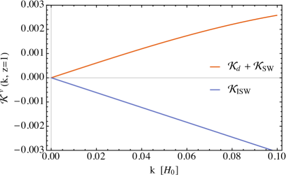
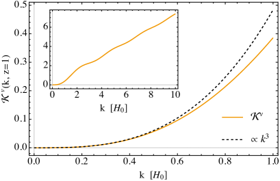
Expanding 𝒦SWsubscript𝒦SW\mathcal{K}_{\rm SW}, 𝒦ISWsubscript𝒦ISW\mathcal{K}_{\rm ISW}, and 𝒦Dsubscript𝒦D\mathcal{K}_{\rm D} separately, the leading order term in the Taylor series expansion is linear in k𝑘k. Therefore, a cancellation between these terms must occur in the limit k0𝑘0k\rightarrow 0. This is the same type of cancellation demonstrated for the primary CMB dipole due to a pure gradient in Ref. [53]. We demonstrate this cancellation analytically in a Universe with matter and a cosmological constant in Appendix C. The cancellation, and the behavior of the full kernel 𝒦v(k,χe)superscript𝒦𝑣𝑘subscript𝜒𝑒\mathcal{K}^{v}(k,\chi_{e}) at z=1𝑧1z=1 for small k𝑘k is shown in figure 2.

Looking at the inset of the right panel in figure 2, we see that the contributions from the spherical Bessel functions in the SW, ISW, and Doppler kernels are evident as oscillations on the linear Doppler contribution. These effects are significant on scales up to of order k10H02×103Mpc1similar-to𝑘10subscript𝐻0similar-to2superscript103superscriptMpc1k\sim 10\ H_{0}\sim 2\times 10^{-3}\ {\rm Mpc}^{-1}.

Refer to caption
Refer to caption
Figure 2: The cancellation at linear order of the three pieces of 𝒦vsuperscript𝒦𝑣\mathcal{K}^{v} as k0𝑘0k\rightarrow 0 in ΛΛ\LambdaCDM. This cancellation can be shown analytically in a universe without radiation (see Appendix C). The leading order behavior is cubic as k0𝑘0k\rightarrow 0 as shown in the right panel.

2.2 Angular decomposition of the effective velocity

The multipole moments of the effective velocity are given by integrating over 𝐧^esubscript^𝐧𝑒{\bf\hat{n}}_{e}

amv(χe)=superscriptsubscript𝑎𝑚𝑣subscript𝜒𝑒absent\displaystyle a_{\ell m}^{v}(\chi_{e})= d2𝐧^eveff(𝐧^e,χe)Ym(𝐧^e)superscript𝑑2subscript^𝐧𝑒subscript𝑣effsubscript^𝐧𝑒subscript𝜒𝑒subscriptsuperscript𝑌𝑚subscript^𝐧𝑒\displaystyle\int d^{2}{\bf\hat{n}}_{e}\ v_{\text{eff}}({\bf\hat{n}}_{e},\chi_{e})\ Y^{*}_{\ell m}({\bf\hat{n}}_{e}) (2.24)
=\displaystyle= id3k(2π)3T(k)Ψ~i(𝐤)𝒦v(k,χe)d2𝐧^eYm(𝐧^e)𝒫1(𝐤^𝐧^e)eiχe𝐤𝐧^e.𝑖superscript𝑑3𝑘superscript2𝜋3𝑇𝑘subscript~Ψ𝑖𝐤superscript𝒦𝑣𝑘subscript𝜒𝑒superscript𝑑2subscript^𝐧𝑒subscriptsuperscript𝑌𝑚subscript^𝐧𝑒subscript𝒫1^𝐤subscript^𝐧𝑒superscript𝑒𝑖subscript𝜒𝑒𝐤subscript^𝐧𝑒\displaystyle\ i\int\frac{d^{3}k}{(2\pi)^{3}}\ T(k)\ \tilde{\Psi}_{i}(\mathbf{k})\ \mathcal{K}^{v}(k,\chi_{e})\int d^{2}{\bf\hat{n}}_{e}\ Y^{*}_{\ell m}({\bf\hat{n}}_{e})\ \mathcal{P}_{1}({\bf\hat{k}}\cdot{\bf\hat{n}}_{e})\ e^{i\chi_{e}{\bf k}\cdot{\bf\hat{n}}_{e}}. (2.25)

The second integral can be written as a triple product of spherical harmonics by expanding the exponential using (A.3) and writing the Legendre polynomials in terms of spherical harmonics using

𝒫(𝐱^𝐱^)=4π2+1m=Ym(𝐱^)Ym(𝐱^).subscript𝒫^𝐱superscript^𝐱4𝜋21superscriptsubscript𝑚subscriptsuperscript𝑌𝑚^𝐱subscript𝑌𝑚superscript^𝐱\mathcal{P}_{\ell}({\bf\hat{x}}\cdot{\bf\hat{x}}^{\prime})=\frac{4\pi}{2\ell+1}\sum_{m=-\ell}^{\ell}Y^{*}_{\ell m}({\bf\hat{x}})\ Y_{\ell m}({\bf\hat{x}}^{\prime}). (2.26)

The integral over 𝐧^esubscript^𝐧𝑒{\bf\hat{n}}_{e} then becomes

d2𝐧^eYm(𝐧^e)[4π3m′′=11Y1m′′(𝐤^)Y1m′′(𝐧^e)][4πij(kχe)m=Ym(𝐤^)Ym(𝐧^e)]superscript𝑑2subscript^𝐧𝑒subscriptsuperscript𝑌𝑚subscript^𝐧𝑒delimited-[]4𝜋3superscriptsubscriptsuperscript𝑚′′11subscriptsuperscript𝑌1superscript𝑚′′^𝐤subscript𝑌1superscript𝑚′′subscript^𝐧𝑒delimited-[]4𝜋superscript𝑖superscriptsubscript𝑗superscript𝑘subscript𝜒𝑒superscriptsubscriptsuperscript𝑚superscriptsuperscriptsubscript𝑌superscriptsuperscript𝑚^𝐤subscriptsuperscript𝑌superscriptsuperscript𝑚subscript^𝐧𝑒\displaystyle\int d^{2}{\bf\hat{n}}_{e}Y^{*}_{\ell m}({\bf\hat{n}}_{e})\left[\frac{4\pi}{3}\sum_{m^{\prime\prime}=-1}^{1}Y^{*}_{1m^{\prime\prime}}({\bf\hat{k}})Y_{1m^{\prime\prime}}({\bf\hat{n}}_{e})\right]\left[4\pi i^{\ell^{\prime}}j_{\ell^{\prime}}(k\chi_{e})\sum_{m^{\prime}=-\ell^{\prime}}^{\ell^{\prime}}Y_{\ell^{\prime}m^{\prime}}({\bf\hat{k}})Y^{*}_{\ell^{\prime}m^{\prime}}({\bf\hat{n}}_{e})\right]
=(4π)23,m,m′′ij(kχe)Y1m′′(𝐤^)Ym(𝐤^)d2𝐧^eYm(𝐧^e)Ym(𝐧^e)Y1m′′(𝐧^e).absentsuperscript4𝜋23subscriptsuperscriptsuperscript𝑚superscript𝑚′′superscript𝑖superscriptsubscript𝑗superscript𝑘subscript𝜒𝑒subscriptsuperscript𝑌1superscript𝑚′′^𝐤subscript𝑌superscriptsuperscript𝑚^𝐤superscript𝑑2subscript^𝐧𝑒subscriptsuperscript𝑌𝑚subscript^𝐧𝑒subscriptsuperscript𝑌superscriptsuperscript𝑚subscript^𝐧𝑒subscript𝑌1superscript𝑚′′subscript^𝐧𝑒\displaystyle=\frac{(4\pi)^{2}}{3}\sum_{\ell^{\prime},m^{\prime},m^{\prime\prime}}i^{\ell^{\prime}}j_{\ell^{\prime}}(k\chi_{e})Y^{*}_{1m^{\prime\prime}}({\bf\hat{k}})Y_{\ell^{\prime}m^{\prime}}({\bf\hat{k}})\int d^{2}{\bf\hat{n}}_{e}Y^{*}_{\ell m}({\bf\hat{n}}_{e})Y^{*}_{\ell^{\prime}m^{\prime}}({\bf\hat{n}}_{e})Y_{1m^{\prime\prime}}({\bf\hat{n}}_{e}). (2.27)

The triple product integral can be expressed in terms of the Clebsch-Gordan coefficients Cm1m2m3123subscriptsuperscriptCsubscript1subscript2subscript3subscript𝑚1subscript𝑚2subscript𝑚3\text{C}^{\ell_{1}\ell_{2}\ell_{3}}_{m_{1}m_{2}m_{3}}:

d2𝐧^eYm(𝐧^e)Ym(𝐧^e)Y1m′′(𝐧^e)=(2+1)(2+1)12πC0001Cmmm′′1.superscript𝑑2subscript^𝐧𝑒subscriptsuperscript𝑌𝑚subscript^𝐧𝑒subscriptsuperscript𝑌superscriptsuperscript𝑚subscript^𝐧𝑒subscript𝑌1superscript𝑚′′subscript^𝐧𝑒212superscript112𝜋subscriptsuperscriptCsuperscript1000subscriptsuperscriptCsuperscript1𝑚superscript𝑚superscript𝑚′′\int d^{2}{\bf\hat{n}}_{e}\ Y^{*}_{\ell m}({\bf\hat{n}}_{e})\ Y^{*}_{\ell^{\prime}m^{\prime}}({\bf\hat{n}}_{e})\ Y_{1m^{\prime\prime}}({\bf\hat{n}}_{e})=\sqrt{\frac{(2\ell+1)(2\ell^{\prime}+1)}{12\pi}}\ \text{C}^{\ell\ell^{\prime}1}_{000}\ \text{C}^{\ell\ell^{\prime}1}_{mm^{\prime}m^{\prime\prime}}. (2.28)

These first coefficients C0001subscriptsuperscriptCsuperscript1000\text{C}^{\ell\ell^{\prime}1}_{000} are only nonzero for =±1superscriptplus-or-minus1\ell^{\prime}=\ell\pm 1. The second coefficients Cmmm′′±1 1subscriptsuperscriptCplus-or-minus11𝑚superscript𝑚superscript𝑚′′\text{C}^{\ell\ \ell\pm 1\ 1}_{mm^{\prime}m^{\prime\prime}} then require that m=m′′msuperscript𝑚superscript𝑚′′𝑚m^{\prime}=m^{\prime\prime}-m for m′′=1,0,1superscript𝑚′′101m^{\prime\prime}=-1,0,1. Therefore, the sums over superscript\ell^{\prime} and msuperscript𝑚m^{\prime} in (2.27) will select six non-zero terms in which (,m)superscriptsuperscript𝑚(\ell^{\prime},m^{\prime}) take the values (+1,1m),(+1,m),(+1,1m),(1,1m),(1,m),(1,1m)11𝑚1𝑚11𝑚11𝑚1𝑚11𝑚(\ell+1,1-m),\ (\ell+1,-m),\ (\ell+1,-1-m),\ (\ell-1,1-m),\ (\ell-1,-m),\ (\ell-1,-1-m). Further, spherical harmonic identities and spherical Bessel recursion relations can then be used to simplify these six terms into just two terms proportional to Ym(𝐤^)subscriptsuperscript𝑌𝑚^𝐤Y^{*}_{\ell m}({\bf\hat{k}}). Equation (2.27) reduces to

4π2+1Ym(𝐤^)[i1j1(kχe)+i+1(+1)j+1(kχe)].4𝜋21subscriptsuperscript𝑌𝑚^𝐤delimited-[]superscript𝑖1subscript𝑗1𝑘subscript𝜒𝑒superscript𝑖11subscript𝑗1𝑘subscript𝜒𝑒\frac{4\pi}{2\ell+1}Y^{*}_{\ell m}({\bf\hat{k}})\left[i^{\ell-1}\ \ell\ j_{\ell-1}(k\chi_{e})+i^{\ell+1}(\ell+1)j_{\ell+1}(k\chi_{e})\right]. (2.29)

Plugging this in for the second integral in equation (2.25) leads to the expression

amv(χe)=d3k(2π)3Δv(k,χe)Ψ~i(𝐤)Ym(𝐤^),superscriptsubscript𝑎𝑚𝑣subscript𝜒𝑒superscript𝑑3𝑘superscript2𝜋3superscriptsubscriptΔ𝑣𝑘subscript𝜒𝑒subscript~Ψ𝑖𝐤subscriptsuperscript𝑌𝑚^𝐤a_{\ell m}^{v}(\chi_{e})=\int\frac{d^{3}k}{(2\pi)^{3}}\ \Delta_{\ell}^{v}(k,\chi_{e})\tilde{\Psi}_{i}(\mathbf{k})Y^{*}_{\ell m}({\bf\hat{k}}), (2.30)

where we have defined the transfer function Δv(k,χe)subscriptsuperscriptΔ𝑣𝑘subscript𝜒𝑒\Delta^{v}_{\ell}(k,\chi_{e}) as

Δv(k,χe)4πi2+1𝒦v(k,zχe)[j1(kχe)(+1)j+1(kχe)]T(k).subscriptsuperscriptΔ𝑣𝑘subscript𝜒𝑒4𝜋superscript𝑖21superscript𝒦𝑣𝑘𝑧subscript𝜒𝑒delimited-[]subscript𝑗1𝑘subscript𝜒𝑒1subscript𝑗1𝑘subscript𝜒𝑒𝑇𝑘\Delta^{v}_{\ell}(k,\chi_{e})\equiv\frac{4\pi\ i^{\ell}}{2\ell+1}\mathcal{K}^{v}(k,z\chi_{e})\left[\ell\ j_{\ell-1}(k\chi_{e})-(\ell+1)j_{\ell+1}(k\chi_{e})\right]T(k). (2.31)

The asymptotic behavior of the transfer function as k𝑘k\rightarrow\infty and k0𝑘0k\rightarrow 0 is given by:

limkΔv(k,χe)subscript𝑘subscriptsuperscriptΔ𝑣𝑘subscript𝜒𝑒\displaystyle\lim_{k\rightarrow\infty}\Delta^{v}_{\ell}(k,\chi_{e}) =\displaystyle= 4πiDv(χe)χeT(k)cos[kχeπ/2],4𝜋superscript𝑖subscript𝐷𝑣subscript𝜒𝑒subscript𝜒𝑒𝑇𝑘𝑘subscript𝜒𝑒𝜋2\displaystyle-4\pi i^{\ell}\frac{D_{v}(\chi_{e})}{\chi_{e}}T(k)\cos\left[k\chi_{e}-\ell\pi/2\right], (2.32)
limk0Δv(k,χe)subscript𝑘0subscriptsuperscriptΔ𝑣𝑘subscript𝜒𝑒\displaystyle\lim_{k\rightarrow 0}\Delta^{v}_{\ell}(k,\chi_{e}) =\displaystyle= 4πi2+1[π(kχe)12Γ[12+]]c3(χe)k3,4𝜋superscript𝑖21delimited-[]𝜋superscript𝑘subscript𝜒𝑒1superscript2Γdelimited-[]12subscript𝑐3subscript𝜒𝑒superscript𝑘3\displaystyle\frac{4\pi\ i^{\ell}}{2\ell+1}\left[\frac{\ell\sqrt{\pi}(k\chi_{e})^{\ell-1}}{2^{\ell}\Gamma[\frac{1}{2}+\ell]}\right]c_{3}(\chi_{e})k^{3}, (2.33)

where in the small-k𝑘k limit we have used the fact that T(0)=1𝑇01T(0)=1 and written the coefficient of the leading order (cubic) term in the Taylor series expansion of 𝒦v(k,zχe)superscript𝒦𝑣𝑘𝑧subscript𝜒𝑒\mathcal{K}^{v}(k,z\chi_{e}) as c3(χe)subscript𝑐3subscript𝜒𝑒c_{3}(\chi_{e}); in the large-k𝑘k limit, T(k)k2proportional-to𝑇𝑘superscript𝑘2T(k)\propto k^{-2}.

3 Simulations

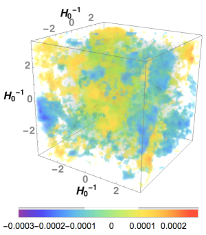
In this section we describe a suite of simulations used to explore the large-scale kSZ effect and provide a concrete example of the relation between the primordial gravitational potential and the effective velocity. This will be used to compute the kSZ signal-to-noise in section 6.2. We create three dimensional realizations of the primordial gravitational potential Ψ(𝐱)Ψ𝐱\Psi({\bf x}) consistent with ΛΛ\LambdaCDM using the method described in Ref. [54] and reviewed in Appendix D. The box size used in each case was L=7H0131.3Gpc𝐿7superscriptsubscript𝐻01similar-to-or-equals31.3GpcL=7H_{0}^{-1}\simeq 31.3\ {\rm Gpc}. One hundred realizations were created at a resolution of 1283superscript1283128^{3}, covering scales down to kmax57.4H0similar-to-or-equalssubscript𝑘max57.4subscript𝐻0k_{\rm max}\simeq 57.4\ H_{0} (λmin484Mpcsimilar-to-or-equalssubscript𝜆min484Mpc\lambda_{\rm min}\simeq 484\ {\rm Mpc}). An example realization is shown in figure 3.

With a set of realizations in hand, we then place a hypothetical observer at the center of the box and generate veff(𝐧^e,χe)subscript𝑣effsubscript^𝐧𝑒subscript𝜒𝑒v_{\rm eff}({\bf\hat{n}}_{e},\chi_{e}) at 505050 equally spaced values of χesubscript𝜒𝑒\chi_{e} at a Healpix resolution [55] of Nside=32subscript𝑁side32N_{\rm side}=32 (12,2881228812,288 equal area pixels of approximately 3.363.363.36 square degrees each). This is done as follows. First, we write the effective velocity as

veff(𝐧^e,χe)=i𝐧^e𝐕(𝐧^e,χe),subscript𝑣effsubscript^𝐧𝑒subscript𝜒𝑒𝑖subscript^𝐧𝑒𝐕subscript^𝐧𝑒subscript𝜒𝑒v_{\rm eff}({\bf\hat{n}}_{e},\chi_{e})=i{\bf\hat{n}}_{e}\cdot{\bf V}({\bf\hat{n}}_{e},\chi_{e}), (3.1)

where

𝐕(𝐧^e,χe)d3k(2π)3[T(k)Ψ~i(𝐤)𝒦v(k,χe)𝐤k]eiχe𝐤𝐧^e.𝐕subscript^𝐧𝑒subscript𝜒𝑒superscript𝑑3𝑘superscript2𝜋3delimited-[]𝑇𝑘subscript~Ψ𝑖𝐤superscript𝒦𝑣𝑘subscript𝜒𝑒𝐤𝑘superscript𝑒𝑖subscript𝜒𝑒𝐤subscript^𝐧𝑒{\bf V}({\bf\hat{n}}_{e},\chi_{e})\equiv\int\frac{d^{3}k}{(2\pi)^{3}}\ \left[T(k)\tilde{\Psi}_{i}({\bf k})\ \mathcal{K}^{v}(k,\chi_{e})\ \frac{\bf k}{k}\right]\ e^{i\chi_{e}{\bf k}\cdot{\bf\hat{n}}_{e}}. (3.2)

The three components of 𝐕(𝐧^e,χe)𝐕subscript^𝐧𝑒subscript𝜒𝑒{\bf V}({\bf\hat{n}}_{e},\chi_{e}) can be straightforwardly evaluated for each realization, at each redshift, using an fast Fourier transform (FFT) algorithm. Plugging back into eq. (3.1) and choosing 𝐧^e𝐳^=cosθsubscript^𝐧𝑒^𝐳𝜃{\bf\hat{n}}_{e}\cdot{\bf\hat{z}}=\cos\theta, 𝐧^e𝐱^=sinθcosϕsubscript^𝐧𝑒^𝐱𝜃italic-ϕ{\bf\hat{n}}_{e}\cdot{\bf\hat{x}}=\sin\theta\cos\phi, and 𝐧^e𝐲^=sinθsinϕsubscript^𝐧𝑒^𝐲𝜃italic-ϕ{\bf\hat{n}}_{e}\cdot{\bf\hat{y}}=\sin\theta\sin\phi, we interpolate the resulting veff(𝐧^e,χe)subscript𝑣effsubscript^𝐧𝑒subscript𝜒𝑒v_{\rm eff}({\bf\hat{n}}_{e},\chi_{e}) at each χesubscript𝜒𝑒\chi_{e} onto the Healpix grid. We then take advantage of the Healpix fast spherical harmonic transform functionality to obtain amv(χe)superscriptsubscript𝑎𝑚𝑣subscript𝜒𝑒a_{\ell m}^{v}(\chi_{e}) at each redshift in each realization.

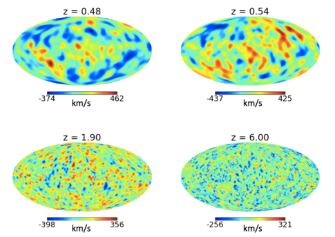
In the right panel of figure 3, we show veff(𝐧^e,χe)subscript𝑣effsubscript^𝐧𝑒subscript𝜒𝑒v_{\rm eff}({\bf\hat{n}}_{e},\chi_{e}) at a variety of redshifts in a single realization. In the top row, we choose two nearby redshifts, where it can be seen by eye that there is a good deal of correlation between the two maps. This is because the same large-scale potential field is responsible for the effective velocities at nearby redshifts. In the bottom row, we choose fairly distant redshifts, where the correlation between the two maps is largely absent. Note also the increasing structure with redshift. This is partially due to the limited resolution of the simulation in this figure, but more physically, there is a real effect due to the redshift transfer function. Based on the smallest structures in the resolution probed in our simulation, 646464 radial samples would capture all radial structures. Empirically, for all but the smallest angular scale structures, the coherence length between redshift slices is sufficiently long to justify our choice of 505050 values of χesubscript𝜒𝑒\chi_{e}.

Refer to caption
Refer to caption
Figure 3: By generating random realizations of Ψ~i(𝐤)subscript~Ψ𝑖𝐤\tilde{\Psi}_{i}({\bf k}), drawn from a Gaussian distribution with power PΨ(k)subscript𝑃Ψ𝑘P_{\Psi}(k), we can construct realizations for veffsubscript𝑣effv_{\text{eff}}. The left panel shows an example realization for Ψi(𝐫)subscriptΨ𝑖𝐫\Psi_{i}({\bf r}), and the resulting maps of veffsubscript𝑣effv_{\text{eff}} at various redshifts, using a resolution of kmax57H0similar-tosubscript𝑘max57subscript𝐻0k_{\text{max}}\sim 57\ H_{0} (λmin484similar-tosubscript𝜆min484\lambda_{\text{min}}\sim 484 Mpc). Notice that correlations are evident between the top two veffsubscript𝑣effv_{\text{eff}} maps at close redshift, but not apparent for widely separated redshifts. Also note the increase in structure at higher redshift.

4 kSZ Tomography

There is a large amount of information lost in performing the line-of-sight integral in eq. (2.1) for the global kSZ signal. One can in principle do far better by cross correlating the kSZ temperature anisotropies with tracers of the electron density field of known redshift. This is evident in the first detections of the kSZ effect, which were made by isolating the component of the temperature anisotropies associated with the pairwise motion of clusters, whose hot interiors harbor a large density of free electrons. In what follows, we assume the most optimistic scenario possible, in which we have perfect knowledge of the electron density field obtained through the measurement of a completely unbiased tracer. We further assume a purely Gaussian primordial power spectrum, consistent with the current constraints from Planck [56].

To tease out the redshift dependence of the large scale kSZ effect, we introduce a window function W(χe,χ¯e)𝑊subscript𝜒𝑒subscript¯𝜒𝑒W(\chi_{e},\bar{\chi}_{e}) that gives the electron density in a set of redshift bins centered on χe=χ¯esubscript𝜒𝑒subscript¯𝜒𝑒\chi_{e}=\bar{\chi}_{e}

δ(𝐧^e,χ¯e)=𝑑χeW(χe,χ¯e)δ(𝐧^e,χe).𝛿subscript^𝐧𝑒subscript¯𝜒𝑒differential-dsubscript𝜒𝑒𝑊subscript𝜒𝑒subscript¯𝜒𝑒𝛿subscript^𝐧𝑒subscript𝜒𝑒\delta({\bf\hat{n}}_{e},\bar{\chi}_{e})=\int d\chi_{e}W(\chi_{e},\bar{\chi}_{e})\delta({\bf\hat{n}}_{e},\chi_{e}). (4.1)

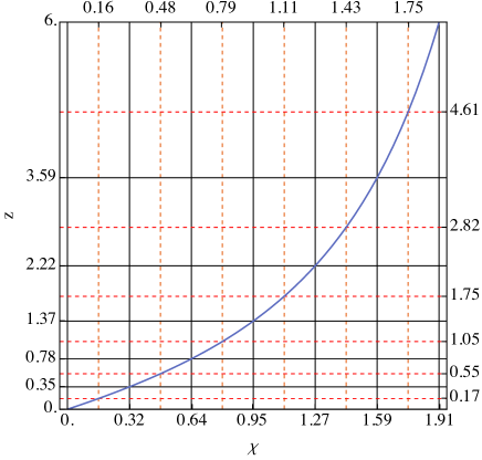
In the following, we use a top-hat window function normalized to unity: 0χ𝑑χW(χ,χ¯)=1superscriptsubscript0subscript𝜒differential-d𝜒𝑊𝜒¯𝜒1\int_{0}^{\chi_{\infty}}d\chi W(\chi,\bar{\chi})=1. We will consider scenarios with 666, 121212, and 242424 redshift bins of equal width, covering the range 0<z<60𝑧60<z<6. The redshift coverage for each bin configuration is shown in Figure 4.

Forming the cross correlation between the kSZ contribution to the CMB temperature anisotropies and the windowed electron density field, we obtain

ΔTT|kSZ(𝐧^e)δ(𝐧^e,χ¯e)=delimited-⟨⟩evaluated-atΔ𝑇𝑇kSZsubscript^𝐧𝑒𝛿subscriptsuperscript^𝐧𝑒subscript¯𝜒𝑒absent\displaystyle\Big{\langle}\frac{\Delta T}{T}\bigg{|}_{\text{kSZ}}({\bf\hat{n}}_{e})\ \delta({\bf\hat{n}}^{\prime}_{e},\bar{\chi}_{e})\Big{\rangle}= σT𝑑χeW(χe,χ¯e)𝑑χea(χe)n¯e(χe)subscript𝜎𝑇differential-dsubscriptsuperscript𝜒𝑒𝑊subscriptsuperscript𝜒𝑒subscript¯𝜒𝑒differential-dsubscript𝜒𝑒𝑎subscript𝜒𝑒subscript¯𝑛𝑒subscript𝜒𝑒\displaystyle\sigma_{T}\int d\chi^{\prime}_{e}\ W(\chi^{\prime}_{e},\bar{\chi}_{e})\ \int d\chi_{e}\ a(\chi_{e})\ \bar{n}_{e}(\chi_{e})
×(1+δ(𝐧^e,χe))veff(𝐧^e,χe)δ(𝐧^e,χe).absentdelimited-⟨⟩1𝛿subscript^𝐧𝑒subscript𝜒𝑒subscript𝑣effsubscript^𝐧𝑒subscript𝜒𝑒𝛿superscriptsubscript^𝐧𝑒subscriptsuperscript𝜒𝑒\displaystyle\times\Big{\langle}(1+\delta({\bf\hat{n}}_{e},\chi_{e}))v_{\rm eff}({\bf\hat{n}}_{e},\chi_{e})\delta({\bf\hat{n}}_{e}^{\prime},\chi^{\prime}_{e})\Big{\rangle}. (4.2)

Now comes a very important step. The correlation function above is defined as an ensemble average. Typically, one is interested in using the measured correlation functions to constrain a statistical model of the ensemble. Here, this is not the case. Instead, we strive to learn information about our particular realization using the cross correlation, which is information that in the former scenario would have been an obstruction to learning about the theoretical model of the ensemble (e.g. cosmic variance). As we wish to learn about large-scale inhomogeneities, the ensemble average in eq.(4.2) should only be taken over small scales, leaving large scales as a fixed deterministic field.
Refer to caption
Figure 4: Redshift is displayed as a function of comoving distance to illustrate the redshift bin configurations. The solid grid lines show the boundaries that define the redshift bins for Nbin=6subscript𝑁bin6N_{\text{bin}}=6. The 12 bin configuration is represented by including the dashed grid lines. It is easy to infer the boundary values for Nbin=24subscript𝑁bin24N_{\text{bin}}=24.

To formulate this idea more precisely, we decompose the primordial potential into long and short wavelength fields, which can be defined in Fourier space as:

Ψi(𝐱)=d3k(2π)3(k)Ψi(𝐤)ei𝐤𝐱,Ψi𝒮(𝐱)=d3k(2π)3𝒮(k)Ψi(𝐤)ei𝐤𝐱,formulae-sequencesuperscriptsubscriptΨ𝑖𝐱superscript𝑑3𝑘superscript2𝜋3𝑘subscriptΨ𝑖𝐤superscript𝑒𝑖𝐤𝐱superscriptsubscriptΨ𝑖𝒮𝐱superscript𝑑3𝑘superscript2𝜋3𝒮𝑘subscriptΨ𝑖𝐤superscript𝑒𝑖𝐤𝐱\Psi_{i}^{\mathcal{L}}({\bf x})=\int\frac{d^{3}k}{(2\pi)^{3}}\mathcal{L}(k)\Psi_{i}({\bf k})e^{i{\bf k}\cdot{\bf x}},\ \ \Psi_{i}^{\mathcal{S}}({\bf x})=\int\frac{d^{3}k}{(2\pi)^{3}}\mathcal{S}(k)\Psi_{i}({\bf k})e^{i{\bf k}\cdot{\bf x}}, (4.3)

such that (k)+𝒮(k)=1𝑘𝒮𝑘1\mathcal{L}(k)+\mathcal{S}(k)=1. A suitable choice could be (k)=ek2/2k2,𝒮(k)=1ek2/2k2formulae-sequence𝑘superscript𝑒superscript𝑘22superscriptsubscript𝑘2𝒮𝑘1superscript𝑒superscript𝑘22superscriptsubscript𝑘2\mathcal{L}(k)=e^{-k^{2}/2k_{*}^{2}},\ \mathcal{S}(k)=1-e^{-k^{2}/2k_{*}^{2}}, although we will implicitly be choosing a step function for (k)𝑘\mathcal{L}(k) in what follows. Below, we imagine that scales larger than k102Mpc1greater-than-or-equivalent-tosubscript𝑘superscript102superscriptMpc1k_{*}\gtrsim 10^{-2}\ {\rm Mpc}^{-1} form the deterministic long field while smaller scales form the stochastic short field. The precise choice of ksubscript𝑘k_{*} does not affect our results because as we show in section 5 and 6 small scales (k102Mpc1much-greater-than𝑘superscript102superscriptMpc1k\gg 10^{-2}\ {\rm Mpc}^{-1}) do not contribute to the signal and large scales (k102Mpc1much-less-than𝑘superscript102superscriptMpc1k\ll 10^{-2}\ {\rm Mpc}^{-1}) do not contribute to the noise.

Because we are working in the linear regime, a long-short split in ΨisubscriptΨ𝑖\Psi_{i} translates into a long-short split in the effective velocity veffsubscript𝑣effv_{\rm eff} and the electron density field δ𝛿\delta, which we therefore decompose as:

veff(𝐧^e,χe)=veff(𝐧^e,χe)+veff𝒮(𝐧^e,χe),δ(𝐧^e,χe)=δ(𝐧^e,χe)+δ𝒮(𝐧^e,χe).formulae-sequencesubscript𝑣effsubscript^𝐧𝑒subscript𝜒𝑒superscriptsubscript𝑣effsubscript^𝐧𝑒subscript𝜒𝑒superscriptsubscript𝑣eff𝒮subscript^𝐧𝑒subscript𝜒𝑒𝛿subscript^𝐧𝑒subscript𝜒𝑒superscript𝛿subscript^𝐧𝑒subscript𝜒𝑒superscript𝛿𝒮subscript^𝐧𝑒subscript𝜒𝑒v_{\text{eff}}({\bf\hat{n}}_{e},\chi_{e})=v_{\text{eff}}^{\mathcal{L}}({\bf\hat{n}}_{e},\chi_{e})+v_{\text{eff}}^{\mathcal{S}}({\bf\hat{n}}_{e},\chi_{e}),\ \ \delta({\bf\hat{n}}_{e},\chi_{e})=\delta^{\mathcal{L}}({\bf\hat{n}}_{e},\chi_{e})+\delta^{\mathcal{S}}({\bf\hat{n}}_{e},\chi_{e}). (4.4)

Substituting these expansions into the ensemble average in eq. (4.2) and extracting the long wavelength fields in the sense described above, we obtain:

(1+δ)veffδ=delimited-⟨⟩1𝛿subscript𝑣effsuperscript𝛿absent\displaystyle\langle(1+\delta)\ v_{\text{eff}}\ \delta^{\prime}\rangle=\ (1+δ+δ𝒮)(veff+veff𝒮)(δ+δ𝒮)delimited-⟨⟩1superscript𝛿superscript𝛿𝒮superscriptsubscript𝑣effsuperscriptsubscript𝑣eff𝒮superscriptsuperscript𝛿superscriptsuperscript𝛿𝒮\displaystyle\langle(1+\delta^{\mathcal{L}}+\delta^{\mathcal{S}})\ (v_{\text{eff}}^{\mathcal{L}}+v_{\text{eff}}^{\mathcal{S}})\ ({\delta^{\prime}}^{\mathcal{L}}+{\delta^{\prime}}^{\mathcal{S}})\rangle
=\displaystyle=\ veffδ+veffδδsuperscriptsubscript𝑣effsuperscriptsuperscript𝛿superscriptsubscript𝑣effsuperscript𝛿superscriptsuperscript𝛿\displaystyle v_{\text{eff}}^{\mathcal{L}}{\delta^{\prime}}^{\mathcal{L}}+v_{\text{eff}}^{\mathcal{L}}\delta^{\mathcal{L}}{\delta^{\prime}}^{\mathcal{L}}
+veffδ𝒮+δveff𝒮+δδveff𝒮+veffδδ𝒮+veffδδ𝒮superscriptsubscript𝑣effdelimited-⟨⟩superscriptsuperscript𝛿𝒮superscriptsuperscript𝛿delimited-⟨⟩superscriptsubscript𝑣eff𝒮superscript𝛿superscriptsuperscript𝛿delimited-⟨⟩superscriptsubscript𝑣eff𝒮superscriptsubscript𝑣effsuperscript𝛿delimited-⟨⟩superscriptsuperscript𝛿𝒮superscriptsubscript𝑣effsuperscriptsuperscript𝛿delimited-⟨⟩superscript𝛿𝒮\displaystyle+v_{\text{eff}}^{\mathcal{L}}\langle{\delta^{\prime}}^{\mathcal{S}}\rangle+{\delta^{\prime}}^{\mathcal{L}}\langle v_{\text{eff}}^{\mathcal{S}}\rangle+\delta^{\mathcal{L}}{\delta^{\prime}}^{\mathcal{L}}\langle v_{\text{eff}}^{\mathcal{S}}\rangle+v_{\text{eff}}^{\mathcal{L}}\delta^{\mathcal{L}}\langle{\delta^{\prime}}^{\mathcal{S}}\rangle+v_{\text{eff}}^{\mathcal{L}}{\delta^{\prime}}^{\mathcal{L}}\langle{\delta}^{\mathcal{S}}\rangle
+veff𝒮δ𝒮δ𝒮delimited-⟨⟩superscriptsubscript𝑣eff𝒮superscript𝛿𝒮superscriptsuperscript𝛿𝒮\displaystyle+\langle v_{\text{eff}}^{\mathcal{S}}\delta^{\mathcal{S}}{\delta^{\prime}}^{\mathcal{S}}\rangle
+veffδ𝒮δ𝒮+δveff𝒮δ𝒮+δveff𝒮δ𝒮+veff𝒮δ𝒮,superscriptsubscript𝑣effdelimited-⟨⟩superscript𝛿𝒮superscriptsuperscript𝛿𝒮superscript𝛿delimited-⟨⟩superscriptsubscript𝑣eff𝒮superscriptsuperscript𝛿𝒮superscriptsuperscript𝛿delimited-⟨⟩superscriptsubscript𝑣eff𝒮superscript𝛿𝒮delimited-⟨⟩superscriptsubscript𝑣eff𝒮superscriptsuperscript𝛿𝒮\displaystyle+v_{\text{eff}}^{\mathcal{L}}\langle\delta^{\mathcal{S}}{\delta^{\prime}}^{\mathcal{S}}\rangle+\delta^{\mathcal{L}}\langle v_{\text{eff}}^{\mathcal{S}}{\delta^{\prime}}^{\mathcal{S}}\rangle+{\delta^{\prime}}^{\mathcal{L}}\langle v_{\text{eff}}^{\mathcal{S}}{\delta}^{\mathcal{S}}\rangle+\langle v_{\text{eff}}^{\mathcal{S}}{\delta^{\prime}}^{\mathcal{S}}\rangle, (4.5)

where δsuperscript𝛿\delta^{\prime} represents δ(𝐧^e,χe)𝛿superscriptsubscript^𝐧𝑒subscriptsuperscript𝜒𝑒\delta({\bf\hat{n}}_{e}^{\prime},\chi^{\prime}_{e}). From our assumption that the short wavelength components are approximately Gaussian, we set the one-point and three-point correlation functions of short wavelength fields to zero, resulting in the final expression:333In any case, significant non-Gaussianity on small scales will not directly mimic the signal we are ultimately after, which is a long wavelength modulation of short wavelength power.

(1+δ)veffδ=delimited-⟨⟩1𝛿subscript𝑣effsuperscript𝛿absent\displaystyle\langle(1+\delta)\ v_{\text{eff}}\ \delta^{\prime}\rangle=\ veffδ+veffδδsuperscriptsubscript𝑣effsuperscriptsuperscript𝛿superscriptsubscript𝑣effsuperscript𝛿superscriptsuperscript𝛿\displaystyle v_{\text{eff}}^{\mathcal{L}}{\delta^{\prime}}^{\mathcal{L}}+v_{\text{eff}}^{\mathcal{L}}\delta^{\mathcal{L}}{\delta^{\prime}}^{\mathcal{L}}
+veff𝒮δ𝒮delimited-⟨⟩superscriptsubscript𝑣eff𝒮superscriptsuperscript𝛿𝒮\displaystyle+\langle v_{\text{eff}}^{\mathcal{S}}{\delta^{\prime}}^{\mathcal{S}}\rangle
+veffδ𝒮δ𝒮+δveff𝒮δ𝒮+δveff𝒮δ𝒮.superscriptsubscript𝑣effdelimited-⟨⟩superscript𝛿𝒮superscriptsuperscript𝛿𝒮superscript𝛿delimited-⟨⟩superscriptsubscript𝑣eff𝒮superscriptsuperscript𝛿𝒮superscriptsuperscript𝛿delimited-⟨⟩superscriptsubscript𝑣eff𝒮superscript𝛿𝒮\displaystyle+v_{\text{eff}}^{\mathcal{L}}\langle\delta^{\mathcal{S}}{\delta^{\prime}}^{\mathcal{S}}\rangle+\delta^{\mathcal{L}}\langle v_{\text{eff}}^{\mathcal{S}}{\delta^{\prime}}^{\mathcal{S}}\rangle+{\delta^{\prime}}^{\mathcal{L}}\langle v_{\text{eff}}^{\mathcal{S}}{\delta}^{\mathcal{S}}\rangle. (4.6)

The terms on the first line give rise to fluctuations on large angular scales, where the primary CMB dominates. We can therefore eliminate this hopelessly unmeasurable term by filtering the CMB on large angular scales 3000less-than-or-similar-to3000\ell\lesssim 3000.444The kSZ effect dominates the CMB temperature anisotropies on scales 3000greater-than-or-equivalent-to3000\ell\gtrsim 3000, as shown in figure 6. The term on the second line gives rise to a statistically isotropic cross power. The terms on the third line give rise to a long wavelength modulation of small-scale power, and will be the focus of what follows. The first of these sources of power asymmetry, veffδ𝒮δ𝒮superscriptsubscript𝑣effdelimited-⟨⟩superscript𝛿𝒮superscriptsuperscript𝛿𝒮v_{\text{eff}}^{\mathcal{L}}\langle\delta^{\mathcal{S}}{\delta^{\prime}}^{\mathcal{S}}\rangle, is far larger than the other two. If we consider a single long (ksuperscript𝑘k^{\mathcal{L}}) and a single short (k𝒮superscript𝑘𝒮k^{\mathcal{S}}) wavelength mode, then noting that the Doppler term dominates veff𝒮superscriptsubscript𝑣eff𝒮v_{\text{eff}}^{\mathcal{S}} and using vδ/kproportional-to𝑣𝛿𝑘v\propto\delta/k, we have δveff𝒮δ𝒮(k/k𝒮)veffδ𝒮δ𝒮veffδ𝒮δ𝒮similar-tosuperscript𝛿delimited-⟨⟩superscriptsubscript𝑣eff𝒮superscriptsuperscript𝛿𝒮superscript𝑘superscript𝑘𝒮superscriptsubscript𝑣effdelimited-⟨⟩superscript𝛿𝒮superscriptsuperscript𝛿𝒮much-less-thansuperscriptsubscript𝑣effdelimited-⟨⟩superscript𝛿𝒮superscriptsuperscript𝛿𝒮\delta^{\mathcal{L}}\langle v_{\text{eff}}^{\mathcal{S}}{\delta^{\prime}}^{\mathcal{S}}\rangle\sim(k^{\mathcal{L}}/k^{\mathcal{S}})v_{\text{eff}}^{\mathcal{L}}\langle\delta^{\mathcal{S}}{\delta^{\prime}}^{\mathcal{S}}\rangle\ll v_{\text{eff}}^{\mathcal{L}}\langle\delta^{\mathcal{S}}{\delta^{\prime}}^{\mathcal{S}}\rangle. We can therefore approximate

(1+δ)veffδsimilar-to-or-equalsdelimited-⟨⟩1𝛿subscript𝑣effsuperscript𝛿absent\displaystyle\langle(1+\delta)\ v_{\text{eff}}\ \delta^{\prime}\rangle\simeq\ veff𝒮δ𝒮+veffδ𝒮δ𝒮,delimited-⟨⟩superscriptsubscript𝑣eff𝒮superscriptsuperscript𝛿𝒮superscriptsubscript𝑣effdelimited-⟨⟩superscript𝛿𝒮superscriptsuperscript𝛿𝒮\displaystyle\langle v_{\text{eff}}^{\mathcal{S}}{\delta^{\prime}}^{\mathcal{S}}\rangle+v_{\text{eff}}^{\mathcal{L}}\langle\delta^{\mathcal{S}}{\delta^{\prime}}^{\mathcal{S}}\rangle, (4.7)

illustrating that there is a statistically isotropic contribution in the first term that depends only on small scales, and an anisotropic contribution in the second term that depends on large scales. The desired signal is captured in the anisotropic power asymmetry, whereas the small scale isotropic component contributes to the noise which is computed next in section 5. Focusing here on the signal, substituting eq. (4.7) into eq. (4.2), and suppressing the 𝒮𝒮\mathcal{S} and \mathcal{L} superscripts, we obtain

ΔTT|kSZ(𝐧^e)δ(𝐧^e,χ¯e)=delimited-⟨⟩evaluated-atΔ𝑇𝑇kSZsubscript^𝐧𝑒𝛿subscriptsuperscript^𝐧𝑒subscript¯𝜒𝑒absent\displaystyle\Big{\langle}\frac{\Delta T}{T}\bigg{|}_{\text{kSZ}}({\bf\hat{n}}_{e})\delta({\bf\hat{n}}^{\prime}_{e},\bar{\chi}_{e})\Big{\rangle}= σT𝑑χea(χe)n¯e(χe)veff(𝐧^e,χe)𝑑χeW(χe,χ¯e)subscript𝜎𝑇differential-dsubscript𝜒𝑒𝑎subscript𝜒𝑒subscript¯𝑛𝑒subscript𝜒𝑒subscript𝑣effsubscript^𝐧𝑒subscript𝜒𝑒differential-dsubscriptsuperscript𝜒𝑒𝑊subscriptsuperscript𝜒𝑒subscript¯𝜒𝑒\displaystyle\sigma_{T}\int d\chi_{e}\ a(\chi_{e})\ \bar{n}_{e}(\chi_{e})\ v_{\rm eff}({\bf\hat{n}}_{e},\chi_{e})\int d\chi^{\prime}_{e}\ W(\chi^{\prime}_{e},\bar{\chi}_{e})
×δ(𝐧^e,χe))δ(𝐧^e,χe)+isotropic.\displaystyle\times\langle\delta({\bf\hat{n}}_{e},\chi_{e}))\ \delta({\bf\hat{n}}^{\prime}_{e},\chi^{\prime}_{e})\rangle+{\rm isotropic}. (4.8)

Assuming the electron distribution traces the dark matter, the electron density correlation function is given by

δ(𝐧^e,χe))δ(𝐧^e,χe)\displaystyle\langle\delta({\bf\hat{n}}_{e},\chi_{e}))\ \delta({\bf\hat{n}}_{e}^{\prime},\chi^{\prime}_{e})\rangle =2+14πCδδ(χe,χe)𝒫(𝐧^e𝐧^e),absentsubscript214𝜋superscriptsubscript𝐶𝛿𝛿subscript𝜒𝑒subscriptsuperscript𝜒𝑒subscript𝒫subscript^𝐧𝑒superscriptsubscript^𝐧𝑒\displaystyle=\sum_{\ell}\frac{2\ell+1}{4\pi}C_{\ell}^{\delta\delta}(\chi_{e},\chi^{\prime}_{e})\mathcal{P}_{\ell}({\bf\hat{n}}_{e}\cdot{\bf\hat{n}}_{e}^{\prime}), (4.9)
withCδδ(χe,χe)withsuperscriptsubscript𝐶𝛿𝛿subscript𝜒𝑒subscriptsuperscript𝜒𝑒\displaystyle\text{with}\ \ \ C_{\ell}^{\delta\delta}(\chi_{e},\chi^{\prime}_{e}) =dkk2(2π)3 4πj(kχe)Pδ(k,χe) 4πj(kχe)Pδ(k,χe),absent𝑑𝑘superscript𝑘2superscript2𝜋34𝜋subscript𝑗𝑘subscript𝜒𝑒subscript𝑃𝛿𝑘subscript𝜒𝑒4𝜋subscript𝑗𝑘subscriptsuperscript𝜒𝑒subscript𝑃𝛿𝑘subscriptsuperscript𝜒𝑒\displaystyle=\int\frac{dk\ k^{2}}{(2\pi)^{3}}\ 4\pi\ j_{\ell}(k\chi_{e})\sqrt{P_{\delta}(k,\chi_{e})}\ 4\pi\ j_{\ell}(k\chi^{\prime}_{e})\sqrt{P_{\delta}(k,\chi^{\prime}_{e})}, (4.10)

where Pδ(k,χe)subscript𝑃𝛿𝑘subscript𝜒𝑒P_{\delta}(k,\chi_{e}) is the non-linear matter power spectrum [57], which was computed using the Cosmicpy package.

We now arrive at the main conclusion of this section. By isolating the statistically anisotropic term in eq. (4), it is possible to measure veffsubscript𝑣effv_{\text{eff}}. Because veffsubscript𝑣effv_{\text{eff}} is related to the primordial potential ΨisubscriptΨ𝑖\Psi_{i} in linear theory by eq. (2.15), this potentially opens a new observational window on large scale inhomogeneities in our Universe. Given a specific model for ΨisubscriptΨ𝑖\Psi_{i}, it is possible to design an optimal filter to extract the power asymmetry described above [33, 35, 45]. However, in the present context of random Gaussian fields, we quantify the power asymmetry by decomposing into power multipoles [58] that capture the anisotropic term in (4.7),

bLM(χ¯e)=d2𝐧^eYLM(𝐧^e)ΔTT|kSZ(𝐧^e)δ(𝐧^e,χ¯e).subscript𝑏𝐿𝑀subscript¯𝜒𝑒superscript𝑑2subscript^𝐧𝑒subscriptsuperscript𝑌𝐿𝑀subscript^𝐧𝑒delimited-⟨⟩evaluated-atΔ𝑇𝑇kSZsubscript^𝐧𝑒𝛿subscript^𝐧𝑒subscript¯𝜒𝑒b_{LM}(\bar{\chi}_{e})=\int d^{2}{\bf\hat{n}}_{e}\ Y^{*}_{LM}({\bf\hat{n}}_{e})\ \Big{\langle}\frac{\Delta T}{T}\bigg{|}_{\text{kSZ}}({\bf\hat{n}}_{e})\ \delta({\bf\hat{n}}_{e},\bar{\chi}_{e})\Big{\rangle}. (4.11)

Let us note that (4.11) is a complete characterization of the signal, as there is no extra information contained in the correlation with 𝐧^e𝐧^esubscript^𝐧𝑒subscriptsuperscript^𝐧𝑒{\bf\hat{n}}_{e}\neq{\bf\hat{n}}^{\prime}_{e}. This is clear from (4) in the limit of gaussian fields. The next step is to expand the long-wavelength effective velocity into multipoles (see section 2.2) using veff(𝐧^e,χe)=,mamv(χe)Ym(𝐧^e)subscript𝑣effsubscript^𝐧𝑒subscript𝜒𝑒subscript𝑚superscriptsubscript𝑎𝑚𝑣subscript𝜒𝑒subscript𝑌𝑚subscript^𝐧𝑒v_{\rm eff}({\bf\hat{n}}_{e},\chi_{e})=\sum_{\ell,m}a_{\ell m}^{v}(\chi_{e})Y_{\ell m}({\bf\hat{n}}_{e}) where amvsuperscriptsubscript𝑎𝑚𝑣a_{\ell m}^{v} is given by (2.30). This makes the angular integral in (4.11) easy to compute as d2𝐧^eYLM(𝐧^e)Ym(𝐧^e)=δLδmMsuperscript𝑑2subscript^𝐧𝑒subscriptsuperscript𝑌𝐿𝑀subscript^𝐧𝑒subscript𝑌𝑚subscript^𝐧𝑒subscript𝛿𝐿subscript𝛿𝑚𝑀\int d^{2}{\bf\hat{n}}_{e}Y^{*}_{LM}({\bf\hat{n}}_{e})Y_{\ell m}({\bf\hat{n}}_{e})=\delta_{\ell L}\delta_{mM}, resulting in the expression,

bLM(χ¯e)=subscript𝑏𝐿𝑀subscript¯𝜒𝑒absent\displaystyle b_{LM}(\bar{\chi}_{e})= =minmax2+14π𝑑k2k2π𝑑χeσTa(χe)n¯e(χe)aLMv(χe)Pδ(k,χe)j(kχe)superscriptsubscriptsubscriptminsubscriptmax214𝜋differential-d𝑘2superscript𝑘2𝜋differential-dsubscript𝜒𝑒subscript𝜎𝑇𝑎subscript𝜒𝑒subscript¯𝑛𝑒subscript𝜒𝑒superscriptsubscript𝑎𝐿𝑀𝑣subscript𝜒𝑒subscript𝑃𝛿𝑘subscript𝜒𝑒subscript𝑗𝑘subscript𝜒𝑒\displaystyle\sum_{\ell=\ell_{\text{min}}}^{\ell_{\text{max}}}\frac{2\ell+1}{4\pi}\int dk\frac{2k^{2}}{\pi}\int d\chi_{e}\ \sigma_{T}\ a(\chi_{e})\ \bar{n}_{e}(\chi_{e})\ a_{LM}^{v}(\chi_{e})\sqrt{P_{\delta}(k,\chi_{e})}\ j_{\ell}(k\chi_{e})
×dχeW(χe,χ¯e)Pδ(k,χe)j(kχe).\displaystyle\times\int d\chi^{\prime}_{e}\ W(\chi^{\prime}_{e},\bar{\chi}_{e})\sqrt{P_{\delta}(k,\chi^{\prime}_{e})}\ j_{\ell}(k\chi^{\prime}_{e}). (4.12)

We therefore see that the power multipoles in each bin are proportional to a weighted integral of the corresponding multipole of the projected effective velocity field. The lower and upper bounds on the summation, (min,maxsubscriptminsubscriptmax\ell_{\text{min}},\ \ell_{\text{max}}), reflect the filtering and resolution scales that might be achievable. By default, we will use (min=3000,max=formulae-sequencesubscriptmin3000subscriptmax\ell_{\text{min}}=3000,\ \ell_{\text{max}}=\infty) unless otherwise stated. The effects of varying these bounds will be discussed in section 8.

5 Cosmic Variance Limited Noise

In this section we estimate the cosmic variance limited noise that we expect for the power multipoles computed in the previous section. However, above, our focus was the statistically anisotropic contribution to the cross correlation, but here we are interested in the statistically isotropic contribution to temperature anisotropies, which depends predominantly on small scales.

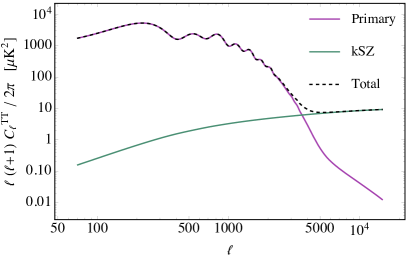
On small angular scales, the late-time kSZ effect is the dominant source of temperature anisotropies in the CMB (see the right panel of figure 6 below). Under the assumption of approximate Gaussianity, and assuming a perfectly unbiased measurement of the electron density field, the primary source of noise is therefore an “accidental” power asymmetry in the cross correlation. We can estimate this through the variance in the power multipoles, which is computed as the coincident limit of the four point function between two powers of ΔTTΔ𝑇𝑇\frac{\Delta T}{T} and two powers of δ𝛿\delta. Specifically, we must compute:

b~LM(χ¯e)b~LM(χ¯e)=delimited-⟨⟩subscriptsuperscript~𝑏𝐿𝑀subscript¯𝜒𝑒subscript~𝑏𝐿𝑀subscript¯𝜒𝑒absent\displaystyle\langle\tilde{b}^{*}_{LM}(\bar{\chi}_{e})\tilde{b}_{LM}(\bar{\chi}_{e})\rangle= d2𝐧^ed2𝐧^eYLM(𝐧^e)YLM(𝐧^e)superscript𝑑2subscript^𝐧𝑒superscript𝑑2subscriptsuperscript^𝐧𝑒subscriptsuperscript𝑌𝐿𝑀subscript^𝐧𝑒subscript𝑌𝐿𝑀subscriptsuperscript^𝐧𝑒\displaystyle\int d^{2}{\bf\hat{n}}_{e}d^{2}{\bf\hat{n}}^{\prime}_{e}\ Y^{*}_{LM}({\bf\hat{n}}_{e})\ Y_{LM}({\bf\hat{n}}^{\prime}_{e})
×ΔTT(𝐧^e)δ(𝐧^e,χ¯e)ΔTT(𝐧^e)δ(𝐧^e,χ¯e),absentdelimited-⟨⟩Δ𝑇𝑇subscript^𝐧𝑒𝛿subscript^𝐧𝑒subscript¯𝜒𝑒Δ𝑇𝑇subscriptsuperscript^𝐧𝑒𝛿subscriptsuperscript^𝐧𝑒subscript¯𝜒𝑒\displaystyle\times\Big{\langle}\frac{\Delta T}{T}({\bf\hat{n}}_{e})\ \delta({\bf\hat{n}}_{e},\bar{\chi}_{e})\ \frac{\Delta T}{T}({\bf\hat{n}}^{\prime}_{e})\ \delta({\bf\hat{n}}^{\prime}_{e},\bar{\chi}_{e})\Big{\rangle}, (5.1)

where we are using tildes on the bLMsubscript𝑏𝐿𝑀b_{LM}’s to indicate that these are not simply the same power multipoles as in (4.12). Instead, the variance here captures the chance power asymmetry that is present in the statistically isotropic contribution to ΔTTΔ𝑇𝑇\frac{\Delta T}{T}, which is sensitive only to small scales where the “conventional” kSZ effect dominates. Since the primary CMB also causes statistical fluctuations in the anisotropic kSZ measurement, we consider both kSZ and primary CMB contributions to ΔTTΔ𝑇𝑇\frac{\Delta T}{T}:

ΔTT=ΔTT|kSZ+ΔTT|pΔ𝑇𝑇evaluated-atΔ𝑇𝑇kSZevaluated-atΔ𝑇𝑇p\frac{\Delta T}{T}=\frac{\Delta T}{T}\bigg{|}_{\text{kSZ}}+\frac{\Delta T}{T}\bigg{|}_{\text{p}} (5.2)

The 4-point function has contributions from all possible 2-point functions and an irreducible/connected piece (which we assume to be negligibly small). Noting that the cross correlation of the primary CMB and the density field is zero, we obtain,

ΔTT(𝐧^e)δ(𝐧^e,χ¯e)ΔTT(𝐧^e)δ(𝐧^e,χ¯e)delimited-⟨⟩Δ𝑇𝑇subscript^𝐧𝑒𝛿subscript^𝐧𝑒subscript¯𝜒𝑒Δ𝑇𝑇subscriptsuperscript^𝐧𝑒𝛿subscriptsuperscript^𝐧𝑒subscript¯𝜒𝑒\displaystyle\Big{\langle}\frac{\Delta T}{T}({\bf\hat{n}}_{e})\ \delta({\bf\hat{n}}_{e},\bar{\chi}_{e})\ \frac{\Delta T}{T}({\bf\hat{n}}^{\prime}_{e})\ \delta({\bf\hat{n}}^{\prime}_{e},\bar{\chi}_{e})\Big{\rangle}
=\displaystyle= ΔTT(𝐧^e)ΔTT(𝐧^e)δ(𝐧^e,χ¯e)δ(𝐧^e,χ¯e)delimited-⟨⟩Δ𝑇𝑇subscript^𝐧𝑒Δ𝑇𝑇subscriptsuperscript^𝐧𝑒delimited-⟨⟩𝛿subscript^𝐧𝑒subscript¯𝜒𝑒𝛿subscriptsuperscript^𝐧𝑒subscript¯𝜒𝑒\displaystyle\Big{\langle}\frac{\Delta T}{T}({\bf\hat{n}}_{e})\ \frac{\Delta T}{T}({\bf\hat{n}}^{\prime}_{e})\Big{\rangle}\Big{\langle}\delta({\bf\hat{n}}_{e},\bar{\chi}_{e})\ \delta({\bf\hat{n}}^{\prime}_{e},\bar{\chi}_{e})\Big{\rangle}
+ΔTT|kSZ(𝐧^e)δ(𝐧^e,χ¯e)ΔTT|kSZ(𝐧^e)δ(𝐧^e,χ¯e).delimited-⟨⟩evaluated-atΔ𝑇𝑇kSZsubscript^𝐧𝑒𝛿subscriptsuperscript^𝐧𝑒subscript¯𝜒𝑒delimited-⟨⟩evaluated-atΔ𝑇𝑇kSZsubscriptsuperscript^𝐧𝑒𝛿subscript^𝐧𝑒subscript¯𝜒𝑒\displaystyle+\Big{\langle}\frac{\Delta T}{T}\bigg{|}_{\text{kSZ}}({\bf\hat{n}}_{e})\ \delta({\bf\hat{n}}^{\prime}_{e},\bar{\chi}_{e})\Big{\rangle}\Big{\langle}\frac{\Delta T}{T}\bigg{|}_{\text{kSZ}}({\bf\hat{n}}^{\prime}_{e})\ \delta({\bf\hat{n}}_{e},\bar{\chi}_{e})\Big{\rangle}. (5.3)

Assuming the electron density field traces dark matter, the electron density autocorrelation function is given by

δ(𝐧^e,χ¯e)δ(𝐧^e,χ¯e)=delimited-⟨⟩𝛿subscript^𝐧𝑒subscript¯𝜒𝑒𝛿subscriptsuperscript^𝐧𝑒subscript¯𝜒𝑒absent\displaystyle\Big{\langle}\delta({\bf\hat{n}}_{e},\bar{\chi}_{e})\ \delta({\bf\hat{n}}^{\prime}_{e},\bar{\chi}_{e})\Big{\rangle}= 2+14πCδδ𝒫(𝐧^e𝐧^e),subscript214𝜋superscriptsubscript𝐶𝛿𝛿subscript𝒫subscript^𝐧𝑒subscriptsuperscript^𝐧𝑒\displaystyle\sum_{\ell}\frac{2\ell+1}{4\pi}\ C_{\ell}^{\delta\delta}\ \mathcal{P}_{\ell}({\bf\hat{n}}_{e}\cdot{\bf\hat{n}}^{\prime}_{e}), (5.4)
withCδδ=withsuperscriptsubscript𝐶𝛿𝛿absent\displaystyle\text{with}\ \ \ C_{\ell}^{\delta\delta}= 𝑑χeW(χe,χ¯e)𝑑χeW(χe,χ¯e)Cδδ(χe,χe)differential-dsubscript𝜒𝑒𝑊subscript𝜒𝑒subscript¯𝜒𝑒differential-dsubscriptsuperscript𝜒𝑒𝑊subscriptsuperscript𝜒𝑒subscript¯𝜒𝑒superscriptsubscript𝐶𝛿𝛿subscript𝜒𝑒subscriptsuperscript𝜒𝑒\displaystyle\int d\chi_{e}\ W(\chi_{e},\bar{\chi}_{e})\int d\chi^{\prime}_{e}\ W(\chi^{\prime}_{e},\bar{\chi}_{e})\ C_{\ell}^{\delta\delta}(\chi_{e},\chi^{\prime}_{e})
=\displaystyle= 𝑑k2k2π𝑑χePδ(k,χe)W(χe,χ¯e)j(kχe)differential-d𝑘2superscript𝑘2𝜋differential-dsubscript𝜒𝑒subscript𝑃𝛿𝑘subscript𝜒𝑒𝑊subscript𝜒𝑒subscript¯𝜒𝑒subscript𝑗𝑘subscript𝜒𝑒\displaystyle\int dk\frac{2k^{2}}{\pi}\int d\chi_{e}\sqrt{P_{\delta}(k,\chi_{e})}W(\chi_{e},\bar{\chi}_{e})j_{\ell}(k\chi_{e})
×dχePδ(k,χe)W(χe,χ¯e)j(kχe)\displaystyle\times\int d\chi^{\prime}_{e}\sqrt{P_{\delta}(k,\chi^{\prime}_{e})}W(\chi^{\prime}_{e},\bar{\chi}_{e})j_{\ell}(k\chi^{\prime}_{e})
similar-to-or-equals\displaystyle\simeq dk+1/2W2(+1/2k,χ¯e)Pδ(k,+1/2k),𝑑𝑘12superscript𝑊212𝑘subscript¯𝜒𝑒subscript𝑃𝛿𝑘12𝑘\displaystyle\int\frac{dk}{\ell+1/2}W^{2}\left(\frac{\ell+1/2}{k},\bar{\chi}_{e}\right)P_{\delta}\left(k,\frac{\ell+1/2}{k}\right), (5.5)

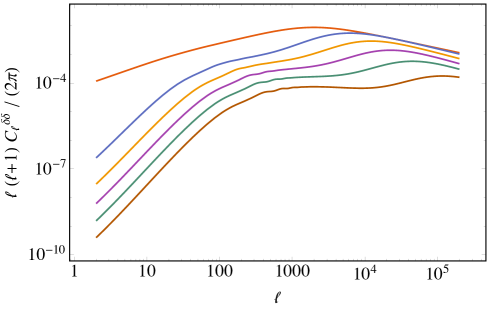
where we used the expression for Cδδ(χe,χe)superscriptsubscript𝐶𝛿𝛿subscript𝜒𝑒subscriptsuperscript𝜒𝑒C_{\ell}^{\delta\delta}(\chi_{e},\chi^{\prime}_{e}) from (4.10), and the Limber approximation [59] in the last line. The quantity Cδδsuperscriptsubscript𝐶𝛿𝛿C_{\ell}^{\delta\delta} is shown in figure 5.

Refer to caption
Figure 5: The non-linear angular matter power spectrum computed in six different redshift bins described by the solid lines in figure 4 from today (top) to z=6𝑧6z=6 (bottom).

The temperature autocorrelation function has contributions from the primary CMB and the conventional kSZ effect. The latter dominates past 3000similar-to3000\ell\sim 3000 and has the following form:

ΔTT|kSZ(𝐧^e)ΔTT|kSZ(𝐧^e)=delimited-⟨⟩evaluated-atevaluated-atΔ𝑇𝑇kSZsubscript^𝐧𝑒Δ𝑇𝑇kSZsubscriptsuperscript^𝐧𝑒absent\displaystyle\Big{\langle}\frac{\Delta T}{T}\bigg{|}_{\text{kSZ}}({\bf\hat{n}}_{e})\ \frac{\Delta T}{T}\bigg{|}_{\text{kSZ}}({\bf\hat{n}}^{\prime}_{e})\Big{\rangle}= 𝑑χeσTa(χe)n¯e(χe)𝑑χeσTa(χe)n¯e(χe)differential-dsubscript𝜒𝑒subscript𝜎𝑇𝑎subscript𝜒𝑒subscript¯𝑛𝑒subscript𝜒𝑒differential-dsubscriptsuperscript𝜒𝑒subscript𝜎𝑇𝑎subscriptsuperscript𝜒𝑒subscript¯𝑛𝑒subscriptsuperscript𝜒𝑒\displaystyle\int d\chi_{e}\sigma_{T}a(\chi_{e})\bar{n}_{e}(\chi_{e})\int d\chi^{\prime}_{e}\sigma_{T}a(\chi^{\prime}_{e})\bar{n}_{e}(\chi^{\prime}_{e})
×q(χe,𝐧^e)q(χe,𝐧^e)absentdelimited-⟨⟩𝑞subscript𝜒𝑒subscript^𝐧𝑒𝑞subscriptsuperscript𝜒𝑒subscriptsuperscript^𝐧𝑒\displaystyle\times\langle q(\chi_{e},{\bf\hat{n}}_{e})q(\chi^{\prime}_{e},{\bf\hat{n}}^{\prime}_{e})\rangle (5.6)
=\displaystyle= 2+14πCTT,kSZ𝒫(𝐧^e𝐧^e),subscript214𝜋superscriptsubscript𝐶𝑇𝑇kSZsubscript𝒫subscript^𝐧𝑒subscriptsuperscript^𝐧𝑒\displaystyle\sum_{\ell}\frac{2\ell+1}{4\pi}\ C_{\ell}^{TT,\text{kSZ}}\ \mathcal{P}_{\ell}({\bf\hat{n}}_{e}\cdot{\bf\hat{n}}^{\prime}_{e}), (5.7)

where q𝐪𝐧^eveff(1+δ)𝑞𝐪subscript^𝐧𝑒subscript𝑣eff1𝛿q\equiv{\bf q}\cdot{\bf\hat{n}}_{e}\equiv v_{\text{eff}}(1+\delta) is the momentum field of free electrons. To obtain an expression for the temperature power spectrum, CTT,kSZsuperscriptsubscript𝐶𝑇𝑇kSZC_{\ell}^{TT,\text{kSZ}}, the key quantity to compute is q(χe,𝐧^e)q(χe,𝐧^e)delimited-⟨⟩𝑞subscript𝜒𝑒subscript^𝐧𝑒𝑞subscriptsuperscript𝜒𝑒subscriptsuperscript^𝐧𝑒\langle q(\chi_{e},{\bf\hat{n}}_{e})q(\chi^{\prime}_{e},{\bf\hat{n}}^{\prime}_{e})\rangle, which is the fourth moment of two δ𝛿\delta’s and two v𝑣v’s. Schematically, qq=vvδδ+2vδ2+vδvδcdelimited-⟨⟩𝑞𝑞delimited-⟨⟩𝑣𝑣delimited-⟨⟩𝛿𝛿2superscriptdelimited-⟨⟩𝑣𝛿2subscriptdelimited-⟨⟩𝑣𝛿𝑣𝛿𝑐\langle qq\rangle=\langle vv\rangle\langle\delta\delta\rangle+2\langle v\delta\rangle^{2}+\langle v\delta v\delta\rangle_{c}, where the subscript c𝑐c denotes the irreducible connected term. The momentum power spectrum, denoted by Pqsubscript𝑃𝑞P_{q}, is typically computed by decomposing the Fourier transform, 𝐪~(𝐤)~𝐪𝐤{\bf\tilde{q}(k)}, into components parallel to 𝐤^^𝐤{\bf\hat{k}}, 𝐪~=𝐤^(𝐪~𝐤^)subscript~𝐪parallel-to^𝐤~𝐪^𝐤{\bf\tilde{q}_{\parallel}=\hat{k}(\tilde{q}\cdot\hat{k}}), and perpendicular to 𝐤^^𝐤{\bf\hat{k}}, 𝐪~=𝐪~𝐤^(𝐪~𝐤^)subscript~𝐪perpendicular-to~𝐪^𝐤~𝐪^𝐤{\bf\tilde{q}_{\perp}=\tilde{q}-{\bf\hat{k}}(\tilde{q}\cdot\hat{k}}) [60]. The longitudinal momentum component does not contribute significantly to CTT,kSZsuperscriptsubscript𝐶𝑇𝑇kSZC_{\ell}^{TT,\text{kSZ}} due to cancellations of positive and negative contributions in the line-of-sight integration. For instance, as shown by Park et al. [61], the longitudinal contribution to CTT,kSZsuperscriptsubscript𝐶𝑇𝑇kSZC_{\ell}^{TT,\text{kSZ}} is more than four orders of magnitude below the transverse contribution for >30003000\ell>3000, so it suffices to only consider Pqsubscript𝑃subscript𝑞perpendicular-toP_{q_{\perp}} in this calculation.

To compute Pqsubscript𝑃subscript𝑞perpendicular-toP_{q_{\perp}}, we use the “standard kSZ model” [61, 62], which incorporates the fully non-linear power spectrum for the density field, Pδnlsuperscriptsubscript𝑃𝛿nlP_{\delta}^{\text{nl}}, but approximates the velocity power spectrum by linear theory Pv=a˙2f2k2Pδlinsubscript𝑃𝑣superscript˙𝑎2superscript𝑓2superscript𝑘2superscriptsubscript𝑃𝛿linP_{v}=\frac{\dot{a}^{2}f^{2}}{k^{2}}P_{\delta}^{\text{lin}} where f=(1+aDΨdDΨda)2𝑓superscript1𝑎subscript𝐷Ψ𝑑subscript𝐷Ψ𝑑𝑎2f=\left(1+\frac{a}{D_{\Psi}}\frac{dD_{\Psi}}{da}\right)^{2}. The resulting expression is

Pq(k,χ)=subscript𝑃subscript𝑞perpendicular-to𝑘𝜒absent\displaystyle P_{q_{\perp}}(k,\chi)= a˙2f211𝑑μdk(2π)2Pδlin(k,χ)Pδnl(k22kkμ+k2,χ)superscript˙𝑎2superscript𝑓2superscriptsubscript11differential-d𝜇𝑑superscript𝑘superscript2𝜋2superscriptsubscript𝑃𝛿linsuperscript𝑘𝜒superscriptsubscript𝑃𝛿nlsuperscript𝑘22𝑘superscript𝑘𝜇superscript𝑘2𝜒\displaystyle\dot{a}^{2}f^{2}\int_{-1}^{1}d\mu\int\frac{dk^{\prime}}{(2\pi)^{2}}\ P_{\delta}^{\text{lin}}(k^{\prime},\chi)\ P_{\delta}^{\text{nl}}(\sqrt{k^{2}-2kk^{\prime}\mu+k^{\prime 2}},\chi)
×(k22kkμ)(1μ2)k22kkμ+k2.absentsuperscript𝑘22𝑘superscript𝑘𝜇1superscript𝜇2superscript𝑘22𝑘superscript𝑘𝜇superscript𝑘2\displaystyle\times\frac{(k^{2}-2kk^{\prime}\mu)(1-\mu^{2})}{k^{2}-2kk^{\prime}\mu+k^{\prime 2}}. (5.8)

This model neglects the velocity-density cross correlation because the geometrical factor attached to this term decreases rapidly at large k𝑘k. Since the kSZ contribution to CTTsuperscriptsubscript𝐶𝑇𝑇C_{\ell}^{TT} that we are interested is sensitive only to high k𝑘k scales, this approximation is valid. Note that this also implies our precise choice of ksubscript𝑘k_{*} in section 4 is irrelevant for the noise calculation. We are also neglecting the non-Gaussian contribution from the connected 4-point function (unimportant on all scales according to [60], but could account for up to 10%percent1010\% of the power spectrum according to [61]). In terms of Pqsubscript𝑃subscript𝑞perpendicular-toP_{q_{\perp}} the temperature power spectrum can be expressed as

CTT,kSZ=superscriptsubscript𝐶𝑇𝑇kSZabsent\displaystyle C_{\ell}^{TT,\text{kSZ}}= 𝑑k2k2π𝑑χeσTa(χe)n¯e(χe)Pq(k,χe)j(kχe)differential-d𝑘2superscript𝑘2𝜋differential-dsubscript𝜒𝑒subscript𝜎𝑇𝑎subscript𝜒𝑒subscript¯𝑛𝑒subscript𝜒𝑒subscript𝑃subscript𝑞perpendicular-to𝑘subscript𝜒𝑒subscript𝑗𝑘subscript𝜒𝑒\displaystyle\int dk\frac{2k^{2}}{\pi}\int d\chi_{e}\sigma_{T}a(\chi_{e})\bar{n}_{e}(\chi_{e})\sqrt{P_{q_{\perp}}(k,\chi_{e})}j_{\ell}(k\chi_{e})
×dχeσTa(χe)n¯e(χe)Pq(k,χe)j(kχe)\displaystyle\times\int d\chi^{\prime}_{e}\sigma_{T}a(\chi^{\prime}_{e})\bar{n}_{e}(\chi^{\prime}_{e})\sqrt{P_{q_{\perp}}(k,\chi^{\prime}_{e})}j_{\ell}(k\chi^{\prime}_{e})
similar-to-or-equals\displaystyle\simeq dk+1/2[σTa(χ)n¯e(χ)]2Pq(k,χ)|χ(+1/2)/k,evaluated-at𝑑𝑘12superscriptdelimited-[]subscript𝜎𝑇𝑎𝜒subscript¯𝑛𝑒𝜒2subscript𝑃subscript𝑞perpendicular-to𝑘𝜒𝜒12𝑘\displaystyle\int\frac{dk}{\ell+1/2}\left[\sigma_{T}a(\chi)\bar{n}_{e}(\chi)\right]^{2}P_{q_{\perp}}(k,\chi)\Big{|}_{\chi\rightarrow(\ell+1/2)/k}, (5.9)

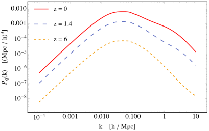
using the Limber approximation [59] again. The functions Pq(k,χ)subscript𝑃subscript𝑞perpendicular-to𝑘𝜒P_{q_{\perp}}(k,\chi) and CTT,kSZsuperscriptsubscript𝐶𝑇𝑇kSZC_{\ell}^{TT,\text{kSZ}} are shown in figure 6. The total temperature power spectrum is a sum of the primary and kSZ contributions, denoted from now on by

CTT=CTT,p+CTT,kSZ.superscriptsubscript𝐶𝑇𝑇superscriptsubscript𝐶𝑇𝑇psuperscriptsubscript𝐶𝑇𝑇kSZC_{\ell}^{TT}=C_{\ell}^{TT,\text{p}}+C_{\ell}^{TT,\text{kSZ}}. (5.10)
Refer to caption
Refer to caption
Figure 6: Left: the power spectrum of the transverse momentum field (5.8). Right: the contributions to the temperature-temperature power spectrum from the primary CMB and the non-linear kSZ effect (5.9).

The second term in eq. (5.3) requires us to compute the cross correlation of the temperature with density. This can be done as follows

ΔTT|kSZ(𝐧^e)δ(𝐧^e,χ¯e)=delimited-⟨⟩evaluated-atΔ𝑇𝑇kSZsubscript^𝐧𝑒𝛿subscriptsuperscript^𝐧𝑒subscript¯𝜒𝑒absent\displaystyle\Big{\langle}\frac{\Delta T}{T}\bigg{|}_{\text{kSZ}}({\bf\hat{n}}_{e})\delta({\bf\hat{n}}^{\prime}_{e},\bar{\chi}_{e})\Big{\rangle}= 𝑑χeσTa(χe)n¯e(χe)veff(𝐧^e,χe)(1+δ(𝐧^e,χe))δ(𝐧^e,χ¯e)differential-dsubscript𝜒𝑒subscript𝜎𝑇𝑎subscript𝜒𝑒subscript¯𝑛𝑒subscript𝜒𝑒delimited-⟨⟩subscript𝑣effsubscript^𝐧𝑒subscript𝜒𝑒1𝛿subscript^𝐧𝑒subscript𝜒𝑒𝛿subscriptsuperscript^𝐧𝑒subscript¯𝜒𝑒\displaystyle-\int d\chi_{e}\sigma_{T}a(\chi_{e})\bar{n}_{e}(\chi_{e})\langle v_{\text{eff}}({\bf\hat{n}}_{e},\chi_{e})(1+\delta({\bf\hat{n}}_{e},\chi_{e}))\delta({\bf\hat{n}}^{\prime}_{e},\bar{\chi}_{e})\rangle
=\displaystyle= 𝑑χeσTa(χe)n¯e(χe)𝑑χeW(χe,χ¯e)veff(𝐧^e,χe)δ(𝐧^e,χe)differential-dsubscript𝜒𝑒subscript𝜎𝑇𝑎subscript𝜒𝑒subscript¯𝑛𝑒subscript𝜒𝑒differential-dsubscriptsuperscript𝜒𝑒𝑊subscriptsuperscript𝜒𝑒subscript¯𝜒𝑒delimited-⟨⟩subscript𝑣effsubscript^𝐧𝑒subscript𝜒𝑒𝛿subscriptsuperscript^𝐧𝑒subscriptsuperscript𝜒𝑒\displaystyle-\int d\chi_{e}\sigma_{T}a(\chi_{e})\bar{n}_{e}(\chi_{e})\int d\chi^{\prime}_{e}W(\chi^{\prime}_{e},\bar{\chi}_{e})\ \langle v_{\text{eff}}({\bf\hat{n}}_{e},\chi_{e})\delta({\bf\hat{n}}^{\prime}_{e},\chi^{\prime}_{e})\rangle
=\displaystyle= 2+14πCTδ𝒫(𝐧^e𝐧^e).subscript214𝜋superscriptsubscript𝐶𝑇𝛿subscript𝒫subscript^𝐧𝑒subscriptsuperscript^𝐧𝑒\displaystyle\sum_{\ell}\frac{2\ell+1}{4\pi}\ C_{\ell}^{T\delta}\ \mathcal{P}_{\ell}({\bf\hat{n}}_{e}\cdot{\bf\hat{n}}^{\prime}_{e}). (5.11)

Assuming approximate Gaussianity, we neglect the three point function vδδdelimited-⟨⟩𝑣𝛿𝛿\langle v\delta\delta\rangle, so only the correlation between veffsubscript𝑣effv_{\text{eff}} and δ𝛿\delta remains. Recall that we are computing the contribution from the small scales, whereas the signal calculation above (see eqs. (4.7),(4)) is only sensitive to large scales. The power spectrum CTδsuperscriptsubscript𝐶𝑇𝛿C_{\ell}^{T\delta} takes the form

CTδ=superscriptsubscript𝐶𝑇𝛿absent\displaystyle C_{\ell}^{T\delta}= dkk2(2π)3𝑑χeσTa(χe)n¯e(χe)Δv(k,χe)PΨ(k)𝑑𝑘superscript𝑘2superscript2𝜋3differential-dsubscript𝜒𝑒subscript𝜎𝑇𝑎subscript𝜒𝑒subscript¯𝑛𝑒subscript𝜒𝑒superscriptsubscriptΔ𝑣𝑘subscript𝜒𝑒subscript𝑃Ψ𝑘\displaystyle-\int\frac{dk\ k^{2}}{(2\pi)^{3}}\int d\chi_{e}\sigma_{T}a(\chi_{e})\bar{n}_{e}(\chi_{e})\Delta_{\ell}^{v}(k,\chi_{e})\sqrt{P_{\Psi}(k)}
×dχe4πPδ(k,χe)W(χe,χ¯e)j(kχe)\displaystyle\times\int d\chi^{\prime}_{e}4\pi\sqrt{P_{\delta}(k,\chi^{\prime}_{e})}W(\chi^{\prime}_{e},\bar{\chi}_{e})j_{\ell}(k\chi^{\prime}_{e})
=\displaystyle= dkk2(2π)3𝑑χeσTa(χe)n¯e(χe)4π𝒦v(k,χe)T(k)kdj(kχe)dχePΨ(k)𝑑𝑘superscript𝑘2superscript2𝜋3differential-dsubscript𝜒𝑒subscript𝜎𝑇𝑎subscript𝜒𝑒subscript¯𝑛𝑒subscript𝜒𝑒4𝜋superscript𝒦𝑣𝑘subscript𝜒𝑒𝑇𝑘𝑘𝑑subscript𝑗𝑘subscript𝜒𝑒𝑑subscript𝜒𝑒subscript𝑃Ψ𝑘\displaystyle-\int\frac{dk\ k^{2}}{(2\pi)^{3}}\int d\chi_{e}\sigma_{T}a(\chi_{e})\bar{n}_{e}(\chi_{e})4\pi\mathcal{K}^{v}(k,\chi_{e})\frac{T(k)}{k}\frac{dj_{\ell}(k\chi_{e})}{d\chi_{e}}\sqrt{P_{\Psi}(k)}
×dχe4πPδ(k,χe)W(χe,χ¯e)j(kχe),\displaystyle\times\int d\chi^{\prime}_{e}4\pi\sqrt{P_{\delta}(k,\chi^{\prime}_{e})}W(\chi^{\prime}_{e},\bar{\chi}_{e})j_{\ell}(k\chi^{\prime}_{e}), (5.12)

where we’ve recalled the expression for Δv(k,χe)superscriptsubscriptΔ𝑣𝑘subscript𝜒𝑒\Delta_{\ell}^{v}(k,\chi_{e}) from eq. (2.31), and used the identity,

j1(kχ)(+1)j+1(kχ)2+1=1kdj(kχ)dχ.subscript𝑗1𝑘𝜒1subscript𝑗1𝑘𝜒211𝑘𝑑subscript𝑗𝑘𝜒𝑑𝜒\frac{\ell\ j_{\ell-1}(k\chi)-(\ell+1)j_{\ell+1}(k\chi)}{2\ell+1}=\frac{1}{k}\frac{dj_{\ell}(k\chi)}{d\chi}. (5.13)

Integrating by parts and using the Limber approximation [59] results in the expression

CTδ=superscriptsubscript𝐶𝑇𝛿absent\displaystyle C_{\ell}^{T\delta}= 𝑑k2k2π𝑑χeσTddχe[a(χe)n¯e(χe)𝒦v(k,χe)]T(k)kPΨ(k)j(kχe)differential-d𝑘2superscript𝑘2𝜋differential-dsubscript𝜒𝑒subscript𝜎𝑇𝑑𝑑subscript𝜒𝑒delimited-[]𝑎subscript𝜒𝑒subscript¯𝑛𝑒subscript𝜒𝑒superscript𝒦𝑣𝑘subscript𝜒𝑒𝑇𝑘𝑘subscript𝑃Ψ𝑘subscript𝑗𝑘subscript𝜒𝑒\displaystyle\int dk\frac{2k^{2}}{\pi}\int d\chi_{e}\sigma_{T}\frac{d}{d\chi_{e}}[a(\chi_{e})\bar{n}_{e}(\chi_{e})\mathcal{K}^{v}(k,\chi_{e})]\frac{T(k)}{k}\sqrt{P_{\Psi}(k)}j_{\ell}(k\chi_{e})
×dχePδ(k,χe)W(χe,χ¯e)j(kχe)\displaystyle\times\int d\chi^{\prime}_{e}\sqrt{P_{\delta}(k,\chi^{\prime}_{e})}W(\chi^{\prime}_{e},\bar{\chi}_{e})j_{\ell}(k\chi^{\prime}_{e}) (5.14)
similar-to-or-equals\displaystyle\simeq dk+1/2σTddχ[a(χ)n¯e(χ)𝒦v(k,χ)]T(k)kPΨ(k)Pδ(k,χ)W(χ,χ¯e)|χ(+1/2)/k.evaluated-at𝑑𝑘12subscript𝜎𝑇𝑑𝑑𝜒delimited-[]𝑎𝜒subscript¯𝑛𝑒𝜒superscript𝒦𝑣𝑘𝜒𝑇𝑘𝑘subscript𝑃Ψ𝑘subscript𝑃𝛿𝑘𝜒𝑊𝜒subscript¯𝜒𝑒𝜒12𝑘\displaystyle\int\frac{dk}{\ell+1/2}\ \sigma_{T}\ \frac{d}{d\chi}[a(\chi)\bar{n}_{e}(\chi)\mathcal{K}^{v}(k,\chi)]\ \frac{T(k)}{k}\ \sqrt{P_{\Psi}(k)P_{\delta}(k,\chi)}\ W(\chi,\bar{\chi}_{e})\Big{|}_{\chi\rightarrow(\ell+1/2)/k}.

Combining all of these pieces, expanding 𝒫(𝐧^e𝐧^e)subscript𝒫subscript^𝐧𝑒subscriptsuperscript^𝐧𝑒\mathcal{P}_{\ell}({\bf\hat{n}}_{e}\cdot{\bf\hat{n}}^{\prime}_{e}) in terms of spherical harmonics using the identity (2.26), the variance in the power multipoles can then be written

b~L2=delimited-⟨⟩superscriptsubscript~𝑏𝐿2absent\displaystyle\langle\tilde{b}_{L}^{2}\rangle= Mb~LMb~LM2L+1subscript𝑀delimited-⟨⟩subscriptsuperscript~𝑏𝐿𝑀subscript~𝑏𝐿𝑀2𝐿1\displaystyle\sum_{M}\frac{\langle\tilde{b}^{*}_{LM}\tilde{b}_{LM}\rangle}{2L+1}
=\displaystyle= ,,m,m,MCTTCδδ+CTδCTδ2L+1|d2𝐧^eYLM(𝐧^e)Ym(𝐧^e)Ym(𝐧^e)|2subscriptsuperscript𝑚superscript𝑚𝑀superscriptsubscript𝐶𝑇𝑇superscriptsubscript𝐶superscript𝛿𝛿superscriptsubscript𝐶𝑇𝛿superscriptsubscript𝐶superscript𝑇𝛿2𝐿1superscriptsuperscript𝑑2subscript^𝐧𝑒subscript𝑌𝐿𝑀subscript^𝐧𝑒subscriptsuperscript𝑌𝑚subscript^𝐧𝑒subscriptsuperscript𝑌superscriptsuperscript𝑚subscript^𝐧𝑒2\displaystyle\sum_{\ell,\ell^{\prime},m,m^{\prime},M}\frac{C_{\ell}^{TT}C_{\ell^{\prime}}^{\delta\delta}+C_{\ell}^{T\delta}C_{\ell^{\prime}}^{T\delta}}{2L+1}\ \Big{|}\int d^{2}{\bf\hat{n}}_{e}Y_{LM}({\bf\hat{n}}_{e})Y^{*}_{\ell m}({\bf\hat{n}}_{e})Y^{*}_{\ell^{\prime}m^{\prime}}({\bf\hat{n}}_{e})\Big{|}^{2}
=\displaystyle= ,[CTTCδδ+CTδCTδ](2+1)(2+1)4π(2L+1)2|C000L|2m,m,M|CmmML|2subscriptsuperscriptdelimited-[]superscriptsubscript𝐶𝑇𝑇superscriptsubscript𝐶superscript𝛿𝛿superscriptsubscript𝐶𝑇𝛿superscriptsubscript𝐶superscript𝑇𝛿212superscript14𝜋superscript2𝐿12superscriptsubscriptsuperscriptCsuperscript𝐿0002subscript𝑚superscript𝑚𝑀superscriptsubscriptsuperscriptCsuperscript𝐿𝑚superscript𝑚𝑀2\displaystyle\sum_{\ell,\ell^{\prime}}[C_{\ell}^{TT}C_{\ell^{\prime}}^{\delta\delta}+C_{\ell}^{T\delta}C_{\ell^{\prime}}^{T\delta}]\ \frac{(2\ell+1)(2\ell^{\prime}+1)}{4\pi(2L+1)^{2}}\ \Big{|}\text{C}^{\ell\ell^{\prime}L}_{000}\Big{|}^{2}\sum_{m,m^{\prime},M}\Big{|}\text{C}^{\ell\ell^{\prime}L}_{mm^{\prime}M}\Big{|}^{2}
=\displaystyle= ,[CTTCδδ+CTδCTδ](2+1)(2+1)4π(2L+1)|C000L|2,subscriptsuperscriptdelimited-[]superscriptsubscript𝐶𝑇𝑇superscriptsubscript𝐶superscript𝛿𝛿superscriptsubscript𝐶𝑇𝛿superscriptsubscript𝐶superscript𝑇𝛿212superscript14𝜋2𝐿1superscriptsubscriptsuperscriptCsuperscript𝐿0002\displaystyle\sum_{\ell,\ell^{\prime}}[C_{\ell}^{TT}C_{\ell^{\prime}}^{\delta\delta}+C_{\ell}^{T\delta}C_{\ell^{\prime}}^{T\delta}]\ \frac{(2\ell+1)(2\ell^{\prime}+1)}{4\pi(2L+1)}\ \Big{|}\text{C}^{\ell\ell^{\prime}L}_{000}\Big{|}^{2}, (5.15)

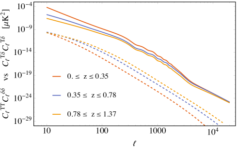
where CmmMLsubscriptsuperscriptCsuperscript𝐿𝑚superscript𝑚𝑀\text{C}^{\ell\ell^{\prime}L}_{mm^{\prime}M} are the Clebsch-Gordan coefficients, and we used the triple product integral identity (see eq. (2.28)) and m,m,M|CmmML|2=2L+1subscript𝑚superscript𝑚𝑀superscriptsubscriptsuperscriptCsuperscript𝐿𝑚superscript𝑚𝑀22𝐿1\sum_{m,m^{\prime},M}\Big{|}\text{C}^{\ell\ell^{\prime}L}_{mm^{\prime}M}\Big{|}^{2}=2L+1. Note that the coefficients C000LsubscriptsuperscriptCsuperscript𝐿000\text{C}^{\ell\ell^{\prime}L}_{000} are only nonzero for ||L+superscript𝐿superscript|\ell-\ell^{\prime}|\leq L\leq\ell+\ell^{\prime} and ++Lsuperscript𝐿\ell+\ell^{\prime}+L even. Figure 7 shows (CTδ)2superscriptsuperscriptsubscript𝐶𝑇𝛿2(C_{\ell}^{T\delta})^{2} plotted in three different redshift bins, and compares this to CTTCδδsuperscriptsubscript𝐶𝑇𝑇superscriptsubscript𝐶𝛿𝛿C_{\ell}^{TT}C_{\ell}^{\delta\delta}. It is clear that the cross term is subdominant by several orders of magnitude for all \ell, and therefore it is sufficient to approximate CTTCδδ+CTδCTδCTTCδδsimilar-tosuperscriptsubscript𝐶𝑇𝑇superscriptsubscript𝐶superscript𝛿𝛿superscriptsubscript𝐶𝑇𝛿superscriptsubscript𝐶superscript𝑇𝛿superscriptsubscript𝐶𝑇𝑇superscriptsubscript𝐶superscript𝛿𝛿C_{\ell}^{TT}C_{\ell^{\prime}}^{\delta\delta}+C_{\ell}^{T\delta}C_{\ell^{\prime}}^{T\delta}\sim C_{\ell}^{TT}C_{\ell^{\prime}}^{\delta\delta}.

Refer to caption
Figure 7: The solid curves are CTTCδδsuperscriptsubscript𝐶𝑇𝑇superscriptsubscript𝐶𝛿𝛿C_{\ell}^{TT}C_{\ell}^{\delta\delta} and the dashed curves are CTδCTδsuperscriptsubscript𝐶𝑇𝛿superscriptsubscript𝐶𝑇𝛿C_{\ell}^{T\delta}C_{\ell}^{T\delta}, which represent the two terms in square brackets in eq. (5.15) evaluated at the same \ell. The redshift ranges indicate sample redshift bins (see figure 4).

The final result for the cosmic variance limited noise estimate is

b~L(χ¯e)2=,=minmax[CTTCδδ(χ¯e)](2+1)(2+1)4π(2L+1)|C000L|2.delimited-⟨⟩subscript~𝑏𝐿superscriptsubscript¯𝜒𝑒2superscriptsubscriptsuperscriptsubscriptminsubscriptmaxdelimited-[]superscriptsubscript𝐶𝑇𝑇superscriptsubscript𝐶superscript𝛿𝛿subscript¯𝜒𝑒212superscript14𝜋2𝐿1superscriptsubscriptsuperscriptCsuperscript𝐿0002\sqrt{\langle\tilde{b}_{L}(\bar{\chi}_{e})^{2}\rangle}=\sqrt{\sum_{\ell,\ell^{\prime}=\ell_{\text{min}}}^{\ell_{\text{max}}}[C_{\ell}^{TT}C_{\ell^{\prime}}^{\delta\delta}(\bar{\chi}_{e})]\ \frac{(2\ell+1)(2\ell^{\prime}+1)}{4\pi(2L+1)}\ \Big{|}\text{C}^{\ell\ell^{\prime}L}_{000}\Big{|}^{2}}. (5.16)

where we have restored an explicit dependence on the redshift bin χ¯esubscript¯𝜒𝑒\bar{\chi}_{e}. Notice that the result is given by a sum over ,superscript\ell,\ell^{\prime}, and recall that the noise captures the accidental power asymmetry which is sensitive only to high \ell. In the spirit of our cosmic variance limited estimate, we can imagine that we have sufficiently filtered out the primary CMB and cleaned the foregrounds. We capture this in the calculation by starting the sum in (5.16) at min=3000subscriptmin3000\ell_{\text{min}}=3000. As previously mentioned, we will employ the default values (min=3000,max=formulae-sequencesubscriptmin3000subscriptmax\ell_{\text{min}}=3000,\ \ell_{\text{max}}=\infty) unless otherwise stated. Results for varying minsubscriptmin\ell_{\text{min}} and maxsubscriptmax\ell_{\text{max}} will be presented in section 8, allowing us to make statements about the detectability with next generation CMB experiments and galaxy surveys.

6 Cosmic Variance Limited Signal to Noise

In this section, we assess the signal to noise for the power multipoles eq. (4.12) in the cosmic variance limit using both a theoretical estimate and the simulations described in section 3. In each case, the signal to noise in each bin χ¯esubscript¯𝜒𝑒\bar{\chi}_{e} is calculated as

SN(χ¯e)=bLM(χ¯e)b~L(χ¯e)2𝑆𝑁subscript¯𝜒𝑒subscript𝑏𝐿𝑀subscript¯𝜒𝑒delimited-⟨⟩subscript~𝑏𝐿superscriptsubscript¯𝜒𝑒2\frac{S}{N}(\bar{\chi}_{e})=\frac{b_{LM}(\bar{\chi}_{e})}{\sqrt{\langle\tilde{b}_{L}(\bar{\chi}_{e})^{2}\rangle}} (6.1)

where bLM(χ¯e)subscript𝑏𝐿𝑀subscript¯𝜒𝑒b_{LM}(\bar{\chi}_{e}) is found using eq. (4.12) and b~L(χ¯e)2delimited-⟨⟩subscript~𝑏𝐿superscriptsubscript¯𝜒𝑒2\sqrt{\langle\tilde{b}_{L}(\bar{\chi}_{e})^{2}\rangle} is given by eq. (5.16).

6.1 RMS Estimate

A simple estimate of the signal is obtained by approximating aLMv(χe)CLv(χe)similar-tosuperscriptsubscript𝑎𝐿𝑀𝑣subscript𝜒𝑒superscriptsubscript𝐶𝐿𝑣subscript𝜒𝑒a_{LM}^{v}(\chi_{e})\sim\sqrt{C_{L}^{v}(\chi_{e})} in eq. (4.12), where CLv(χe)superscriptsubscript𝐶𝐿𝑣subscript𝜒𝑒C_{L}^{v}(\chi_{e}) is the power spectrum associated with the large-scale velocity, given by

CLv(χe)=0kmaxk2dk(2π)3PΨ(k)|ΔLv(k,χe)|2superscriptsubscript𝐶𝐿𝑣subscript𝜒𝑒superscriptsubscript0subscript𝑘maxsuperscript𝑘2𝑑𝑘superscript2𝜋3subscript𝑃Ψ𝑘superscriptsubscriptsuperscriptΔ𝑣𝐿𝑘subscript𝜒𝑒2C_{L}^{v}(\chi_{e})=\int_{0}^{k_{\text{max}}}\frac{k^{2}dk}{(2\pi)^{3}}P_{\Psi}(k)|\Delta^{v}_{L}(k,\chi_{e})|^{2} (6.2)

with ΔLv(k,χe)subscriptsuperscriptΔ𝑣𝐿𝑘subscript𝜒𝑒\Delta^{v}_{L}(k,\chi_{e}) given by eq. (2.31). This necessarily yields an overestimate of the signal, since in reality aL0v(χe)superscriptsubscript𝑎𝐿0𝑣subscript𝜒𝑒a_{L0}^{v}(\chi_{e}) will vary over over the window functions leading to partial cancellation, while here we are assuming that it always takes its (positive definite) RMS value. By comparing with simulations in the following subsection, we show that this approximation gives a good estimate in the limit of thin window functions W(χe,χ¯e)𝑊subscript𝜒𝑒subscript¯𝜒𝑒W(\chi_{e},\bar{\chi}_{e}) (in the context of this paper, this is equivalent to the limit of many redshift bins).

Before proceeding, we can assess which scales form the dominant contribution to eq. (6.2). The upper limit of integration in eq. (6.2), kmaxsubscript𝑘maxk_{\text{max}}, corresponds to the smallest scale, λmin=2π/kmaxsubscript𝜆min2𝜋subscript𝑘max\lambda_{\text{min}}=2\pi/k_{\text{max}}, that contributes to the signal. Formally, kmaxsubscript𝑘maxk_{\text{max}}\rightarrow\infty, but we can adjust the cutoff to include only the long modes discussed above. In figure 8 we show CLvsuperscriptsubscript𝐶𝐿𝑣C_{L}^{v} at z=1𝑧1z=1 as a function of kmaxsubscript𝑘maxk_{\rm max}. Vertical lines indicate λmin=10,102,103Mpcsubscript𝜆min10superscript102superscript103Mpc\lambda_{\text{min}}=10,10^{2},10^{3}\ {\rm Mpc}. Here, we see that for a number of power multipoles, the relevant signal is obtained almost entirely from scales 102103Mpcsimilar-toabsentsuperscript102superscript103Mpc\sim 10^{2}-10^{3}\ {\rm Mpc}.

Refer to caption
Figure 8: The effective velocity contribution to the signal described in eq. (6.2) versus kmaxsubscript𝑘maxk_{\text{max}} in units of H0subscript𝐻0H_{0}, which refers to the upper bound on the integral. Notice that the contribution mainly comes from large scales (small k𝑘k) for low L𝐿L. The vertical lines indicate scales equal to 1 Gpc, 100 Mpc, and 10 Mpc from left to right.

Putting everything together, applying the Limber approximation [59], and choosing M=0𝑀0M=0 under the assumption that all other M𝑀M will statistically be the same, the final expression for the signal becomes

bL0(χ¯e)=minmax2+14πdχχ2σTa(χ)n¯e(χ)CLv(χ)W(χ,χ¯e)Pδ(+1/2χ,χ).similar-to-or-equalssubscript𝑏𝐿0subscript¯𝜒𝑒superscriptsubscriptsubscriptminsubscriptmax214𝜋𝑑𝜒superscript𝜒2subscript𝜎𝑇𝑎𝜒subscript¯𝑛𝑒𝜒superscriptsubscript𝐶𝐿𝑣𝜒𝑊𝜒subscript¯𝜒𝑒subscript𝑃𝛿12𝜒𝜒b_{L0}(\bar{\chi}_{e})\simeq\sum_{\ell=\ell_{\text{min}}}^{\ell_{\text{max}}}\frac{2\ell+1}{4\pi}\int\frac{d\chi}{\chi^{2}}\ \sigma_{T}\ a(\chi)\ \bar{n}_{e}(\chi)\ \sqrt{C_{L}^{v}(\chi)}\ W(\chi,\bar{\chi}_{e})\ P_{\delta}\left(\frac{\ell+1/2}{\chi},\chi\right). (6.3)

We compute the signal eq. (6.3) and noise eq. (5.16) for the Nbin=6, 12,and 24subscript𝑁bin612and24N_{\text{bin}}=6,\ 12,\ \text{and}\ 24 top-hat bin configurations with redshift ranges summarized in figure 4. We show the results for the 6-bin configuration in figure 9. Each plot has four curves. The solid red curve is the RMS signal with kmaxsubscript𝑘maxk_{\text{max}}\rightarrow\infty, the dotted orange line is the cosmic variance limited noise, the short dashed blue line is the RMS signal computed for kmax=278H0subscript𝑘max278subscript𝐻0k_{\text{max}}=278\ H_{0} (λmin=100subscript𝜆min100\lambda_{\text{min}}=100 Mpc), and the long dashed green curve is the signal computed for kmax=2780H0subscript𝑘max2780subscript𝐻0k_{\text{max}}=2780\ H_{0} (λmin=10subscript𝜆min10\lambda_{\text{min}}=10 Mpc). Comparing the three signal curves we see that except in the lowest redshift bin at high L𝐿L, the signal is composed primarily of long wavelength modes (λ>100𝜆100\lambda>100 Mpc), as expected. The amplitude of the signal varies by roughly an order of magnitude between the lowest and highest redshift bin, and is strongest at low L𝐿L and low redshift. Both the signal and noise are relatively flat over the plotted range in L𝐿L. Most importantly though, the signal is 2-3 orders of magnitude larger than the noise!
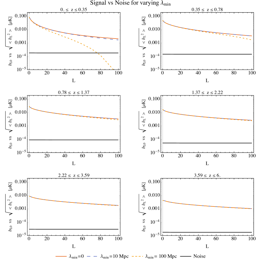
Refer to caption
Figure 9: The signal (6.3) is shown in six redshift bins, calculated for three different scales: kmax=278H0subscript𝑘max278subscript𝐻0k_{\text{max}}=278\ H_{0} (λmin=100subscript𝜆min100\lambda_{\text{min}}=100 Mpc) [orange, short dash], kmax=2780H0subscript𝑘max2780subscript𝐻0k_{\text{max}}=2780\ H_{0} (λmin=10subscript𝜆min10\lambda_{\text{min}}=10 Mpc) [blue, long dash], and kmax=subscript𝑘maxk_{\text{max}}=\infty (λmin=0subscript𝜆min0\lambda_{\text{min}}=0) [red, solid]. The solid black line is the noise estimate b~L2delimited-⟨⟩superscriptsubscript~𝑏𝐿2\sqrt{\langle\tilde{b}_{L}^{2}\rangle} (eq. (5.16)), which falls well below the estimated signal for this configuration. The summation bounds employed for the signal and noise calculations are (min=3000,max=formulae-sequencesubscriptmin3000subscriptmax\ell_{\text{min}}=3000,\ \ell_{\text{max}}=\infty).

To compare the result for the 121212 and 242424 bin configurations, in figure 10 we show the signal to noise eq. (6.1) at L=1𝐿1L=1 and L=50𝐿50L=50 as a function of comoving distance. Increasing the number of bins by a factor of 2 results in a decrease in the signal-to-noise by a factor of 2similar-toabsent2\sim\sqrt{2}. This is true for all L𝐿L. We therefore conclude that a signal can in principle be measured in the cosmic variance limit at high signal to noise for a large number of redshift bins Nbinssubscript𝑁binsN_{\rm bins} at a variety of scales L𝐿L.

Refer to caption
Figure 10: The bullet points (square, circle, triangle) represent the signal-to-noise (eq. (6.1)) in each bin for Nbin=(6,12,24)subscript𝑁bin61224N_{\text{bin}}=(6,12,24), plotted against χ𝜒\chi at the midpoint of the bin. The solid top curves are for L=1𝐿1L=1 and the bottom dashed curves are for L=50𝐿50L=50. The signal and noise were computed using eq. (6.3) and (5.16), employing summation bounds (min=3000,max=formulae-sequencesubscriptmin3000subscriptmax\ell_{\text{min}}=3000,\ \ell_{\text{max}}=\infty), and with kmaxsubscript𝑘maxk_{\text{max}}\rightarrow\infty in eq. (6.2).

6.2 Comparing with the signal from simulations

The above calculation is an over-estimate of the signal, as it assumes the velocity field is positive definite and given by its RMS value. In particular, it does not account for partial cancellations along the line of sight. To take this into account, we can compute the signal from eq. (4.12) using the effective velocity field computed from the simulations described in section 3. Using an interpolating function for amv(χe)superscriptsubscript𝑎𝑚𝑣subscript𝜒𝑒a_{\ell m}^{v}(\chi_{e}) constructed from the veffsubscript𝑣effv_{\rm eff} map in each of the 50 redshift bins, we compute eq. (4.12) directly for 100 realizations at a resolution of kmax57.4H0similar-tosubscript𝑘max57.4subscript𝐻0k_{\text{max}}\sim 57.4\ H_{0} for the 6 and 12 bin configurations. Below we only present results for bL0subscript𝑏𝐿0b_{L0}; other values of M𝑀M have identical statistical properties.

Figures 11 and 12 shows the signal to noise computed using simulations, in comparison to the one estimated from theory with eq. (6.2) computed using the integration limit kmax57.4H0similar-tosubscript𝑘max57.4subscript𝐻0k_{\text{max}}\sim 57.4\ H_{0} corresponding to the simulation resolution. We plot L<10𝐿10L<10, which is accurately captured for the resolution we consider (see figure 8). Notice that the solid curves, showing the predicted signal based on our theory calculation, are always higher than the average signal from the realizations. This is due to a difference in the order of operations. In our estimation in (6.3) we have averaged over aL0(χe)subscript𝑎𝐿0subscript𝜒𝑒a_{L0}(\chi_{e}) prior to integrating over χesubscript𝜒𝑒\chi_{e}, whereas the signal computed from the realizations integrates over χesubscript𝜒𝑒\chi_{e} first and then averages. Since aL0(χe)subscript𝑎𝐿0subscript𝜒𝑒a_{L0}(\chi_{e}) is an oscillating function that takes positive and negative values, there can be cancellation upon integration over χesubscript𝜒𝑒\chi_{e}. This cancellation can be minimized by using smaller redshift bins, which results in a smaller range of integration and a lesser chance for cancellation. This can be noticed empirically as the agreement between realizations and theory is better for the 12 bin configuration than the 6 bin. In summary, the realizations approach the theory estimation for more bins as a result of having less variation in aLMsubscript𝑎𝐿𝑀a_{LM} over the bin.

Refer to caption
Figure 11: The signal-to-noise (eq. (6.1)) computed using simulations, in comparison to the RMS estimate (solid curves), in 6 redshift bins (see figure 4). The points represent the standard deviation of the 100 realizations, and the error bars denote the standard error of the standard deviation. These simulations have a resolution of λmin484similar-tosubscript𝜆min484\lambda_{\text{min}}\sim 484 Mpc and utilized the default summation bounds (min=3000,max=formulae-sequencesubscriptmin3000subscriptmax\ell_{\text{min}}=3000,\ \ell_{\text{max}}=\infty) for the signal and noise calculations.
Refer to caption
Figure 12: [The same as Figure 11 but for 12 redshift bins]. The signal-to-noise (eq. (6.1)) computed using simulations, in comparison to the RMS estimate (solid curves), in 12 redshift bins (see figure 4). The points represent the standard deviation of the 100 realizations, and the error bars denote the standard error of the standard deviation. These simulations have a resolution of λmin484similar-tosubscript𝜆min484\lambda_{\text{min}}\sim 484 Mpc and utilized the default summation bounds (min=3000,max=formulae-sequencesubscriptmin3000subscriptmax\ell_{\text{min}}=3000,\ \ell_{\text{max}}=\infty) for the signal and noise calculations.

7 Mode counting

With an understanding of this signal in hand, we now want to estimate how many modes one could conceivably measure in the cosmic variance limit. Let’s consider scales λ>100𝜆100\lambda>100 Mpc, of order the BAO scale. This corresponds to kmax=278H0subscript𝑘max278subscript𝐻0k_{\text{max}}=278\ H_{0} and Lmaxπ/θπχdec/λmin=kmaxχdec/2437similar-tosubscript𝐿max𝜋𝜃similar-to𝜋subscript𝜒decsubscript𝜆minsubscript𝑘maxsubscript𝜒dec2similar-to437L_{\text{max}}\sim\pi/\theta\sim\pi\chi_{\text{dec}}/\lambda_{\text{min}}=k_{\text{max}}\chi_{\text{dec}}/2\sim 437. On this scale and larger, the primary CMB contains L437(2L+1)=191843superscriptsubscript𝐿4372𝐿1191843\sum_{L}^{437}({2L+1})=191843 modes.

For the kSZ effect considered here, the sum over 2L+12𝐿12L+1 is performed in each bin, therefore one might naively guess that it is possible to get Nbinsubscript𝑁binN_{\text{bin}} times more modes than the primary CMB. However, a more careful estimate needs to be done because the value of Lmaxsubscript𝐿maxL_{\text{max}} varies in each bin depending on the size of the signal. Consider the signal-to-noise, described by the ratio of (6.3) and (5.16), for the scales considered here (see eq. (6.2) and use kmax=278H0subscript𝑘max278subscript𝐻0k_{\text{max}}=278\ H_{0}). For Nbinsubscript𝑁binN_{\text{bin}} bins, in each bin, the value of Lmaxsubscript𝐿maxL_{\text{max}} up to which modes can be measured is found by ensuring that

  1. 1.

    For L<Lmax𝐿subscript𝐿maxL<L_{\text{max}}, the signal-to-noise is bigger than 1.

  2. 2.

    For L<Lmax𝐿subscript𝐿maxL<L_{\text{max}}, the signal is dominated by modes larger than 100100100 Mpc. More precisely, bL0kmax>0.95bL0superscriptsubscript𝑏𝐿0subscript𝑘max0.95superscriptsubscript𝑏𝐿0b_{L0}^{k_{\text{max}}}>0.95b_{L0}^{\infty} for kmax=278H0subscript𝑘max278subscript𝐻0k_{\text{max}}=278\ H_{0}.333The 95%percent9595\% criteria is arbitrary.

Table 1 shows the values of Lmaxsubscript𝐿maxL_{\text{max}} computed in each bin for the 6, 12 and 24 bin configurations. In every case, it was a failure of criteria (2.) that determined Lmaxsubscript𝐿maxL_{\text{max}}, as the signal-to-noise is always much bigger than 1 for this range in L𝐿L. Notice that by doubling the bin size, we approximately double the number of modes. This allows us to extrapolate our results from the three bin configurations.

Nbinsubscript𝑁binN_{\text{bin}} Lmaxsubscript𝐿maxL_{\text{max}} binLLmax(2L+1)subscriptbinsuperscriptsubscript𝐿subscript𝐿max2𝐿1\sum\limits_{\text{bin}}\sum\limits_{L}^{L_{\text{max}}}({2L+1})
6 6, 32, 55, 78, 100, 123 36086
12 4, 16, 28, 39, 51, 62, 73, 85, 96, 107, 118, 131 74946
24 3, 8, 14, 20, 25, 31, 37, 42, 48, 54, 59, 65, 71, 76, 82, 88, 93, 99,  105, 110, 116, 121, 130, 132 150853
Table 1: Number of modes

Figure 13 shows how the number of modes increases with Nbinsubscript𝑁binN_{\text{bin}} based on our estimates using 6, 12 and 24 bins. Extrapolating the data points to higher values of Nbinsubscript𝑁binN_{\text{bin}} shows that at least 30 bins are needed to match the number of modes in the primary CMB. The same increasing trend should continue until Nbin50similar-tosubscript𝑁bin50N_{\text{bin}}\sim 50 (producing 309656 modes), at which point we estimate that the signal-to-noise will drop below 1 in the high redshift bins, thus failing to satisfy criteria (1.), and causing a less rapid increase in the number of modes as a function of Nbinsubscript𝑁binN_{\text{bin}}. Therefore, this method can theoretically achieve more modes than the primary CMB. However, note that within the observable Universe, on scales λ>100𝜆100\lambda>100 Mpc, there are approximately (χdeckmax/(2π))32.7×106similar-tosuperscriptsubscript𝜒decsubscript𝑘max2𝜋32.7superscript106\left(\chi_{\text{dec}}k_{\text{max}}/(2\pi)\right)^{3}\sim 2.7\times 10^{6} total modes. Thus, while remaining competitive with the primary CMB, the proposed method still falls about an order of magnitude short of the total number of possible modes. In addition, because they provide at least partially independent constraints, combining the information from the primary CMB and the information from kSZ tomography can in principle constrain a larger number of modes than either individually.
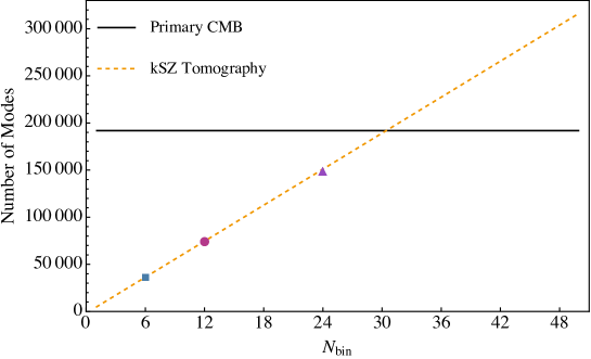
Refer to caption
Figure 13: The bullet points show the number of modes that can possibly be measured using Nbin=subscript𝑁binabsentN_{\text{bin}}= 6, 12, and 24. Extrapolating these data points (dashed line) indicates that we need at least 30 bins to match the number of modes in the primary CMB at 437437\ell\leq 437 (solid line). These calculations were performed with the default summation bounds (min=3000,max=formulae-sequencesubscriptmin3000subscriptmax\ell_{\text{min}}=3000,\ \ell_{\text{max}}=\infty).

8 Detectability

How close can we get to the cosmic variance limited result with the next generation of CMB experiments and galaxy surveys? Although a complete treatment is beyond the scope of this paper, we can give a rough estimate here. The two parameters affecting detectability in the analysis above are the filtering scale minsubscriptmin\ell_{\text{min}} and resolution maxsubscriptmax\ell_{\text{max}}. The filtering scale is a parameter which can be optimized in any hypothetical analysis. By varying maxsubscriptmax\ell_{\text{max}}, we can define a rough target for the instrumental noise, resolution, and foreground residuals necessary for a detection to be made.

Previously, we had made the fiducial choice min=3000subscriptmin3000\ell_{\text{min}}=3000, which is roughly the angular scale on which the kSZ power surpasses that in the primary CMB. Here, we will explore the filtering scales min=2, 1000, 3000subscriptmin210003000\ell_{\text{min}}=2,\ 1000,\ 3000. In addition, we chose maxsubscriptmax\ell_{\text{max}}\rightarrow\infty, corresponding to the cosmic variance limit. Here, we consider a low-resolution scenario with max=3000subscriptmax3000\ell_{\text{max}}=3000 and high-resolution scenario with max=5000subscriptmax5000\ell_{\text{max}}=5000.

Starting with the high resolution scenario, in figure 14, we show the signal and noise for six redshift bins, choosing min=2, 1000, 3000subscriptmin210003000\ell_{\text{min}}=2,\ 1000,\ 3000 and max=5000subscriptmax5000\ell_{\text{max}}=5000. The choice min=2subscriptmin2\ell_{\text{min}}=2, where the noise includes the primary CMB, is clearly not optimal as the signal to noise is at most close to one. Raising the filtering scale to min=1000subscriptmin1000\ell_{\text{min}}=1000, the signal drops slightly (an effect that is more pronounced at low redshift), but the noise drops by an order of magnitude, raising the signal to noise accordingly. Raising the filtering scale further to min=3000subscriptmin3000\ell_{\text{min}}=3000 again further increases the signal to noise. Clearly, removing as much of the primary CMB as possible through filtering is the choice that will optimize signal to noise. Comparing the dotted curves (min=3000subscriptmin3000\ell_{\text{min}}=3000) with figure 9, reducing max=subscriptmax\ell_{\text{max}}=\infty to max=5000subscriptmax5000\ell_{\text{max}}=5000 degrades the signal to noise by about a factor of 101001010010-100, with the degredation more pronounced in the large-redshift bins. Nevertheless, the signal to noise is still S/N10100similar-to𝑆𝑁10100S/N\sim 10-100 over a significant range in L𝐿L.

Refer to caption
Figure 14: The signal (6.3) (coloured lines) and noise (5.16) (black lines) are shown in six redshift bins, computed with kmax=subscript𝑘maxk_{\text{max}}=\infty and max=5000subscriptmax5000\ell_{\text{max}}=5000. We consider different filter scales: min=2subscriptmin2\ell_{\text{min}}=2 (solid), min=1000subscriptmin1000\ell_{\text{min}}=1000 (long dash), min=3000subscriptmin3000\ell_{\text{min}}=3000 (short dash).
Refer to caption
Figure 15: The signal (6.3) (dashed) and noise (5.16) (solid) are shown in six redshift bins, computed with kmax=subscript𝑘maxk_{\text{max}}=\infty, min=3000subscriptmin3000\ell_{\text{min}}=3000, and max=3000subscriptmax3000\ell_{\text{max}}=3000.

Moving on to the low resolution scenario, in figure 15 we show the signal and noise for six redshift bins, choosing min=1000subscriptmin1000\ell_{\text{min}}=1000 and max=3000subscriptmax3000\ell_{\text{max}}=3000. Here, it can be seen that the signal-to-noise is significant only for the low redshift bins, and reaches at most S/N10similar-to𝑆𝑁10S/N\sim 10.

With these results, we can map the low and high resolution scenarios to a rough set of experimental requirements. In particular, we consider CMB instrumental noise, foreground residuals, finite resolution, and galaxy shot noise. The treatment of a number of important systematics is beyond the scope of this paper. We assume that the instrumental noise contribution to the CMB temperature is gaussian and uniform on the sky,555This is clearly incorrect, and spatially varying noise will be an important systematic to assess in the future. gaussian beams, and that foreground residuals in the cleaned data product used for the analysis can be modelled as a uniform gaussian random field. Under these assumptions, the measured CMB temperature power spectrum is modelled as:

CTT=(CTT,kSZ+CTT,p+NCMB+FCMB)exp[(+1)θFWHM28ln2],superscriptsubscript𝐶𝑇𝑇superscriptsubscript𝐶𝑇𝑇kSZsuperscriptsubscript𝐶𝑇𝑇psuperscriptsubscript𝑁CMBsuperscriptsubscript𝐹CMB1superscriptsubscript𝜃FWHM282C_{\ell}^{TT}=\left(C_{\ell}^{TT,\text{kSZ}}+C_{\ell}^{TT,\text{p}}+N_{\ell}^{\rm CMB}+F_{\ell}^{\rm CMB}\right)\exp\left[\frac{\ell(\ell+1)\theta_{\rm FWHM}^{2}}{8\ln 2}\right], (8.1)

where θFWHMsubscript𝜃FWHM\theta_{\rm FWHM} is the full-width at half-maximum of the Gaussian beam in radians. The noise and foreground contributions are

NCMB=(σNθFWHM)2,superscriptsubscript𝑁CMBsuperscriptsubscript𝜎𝑁subscript𝜃FWHM2N_{\ell}^{\rm CMB}=(\sigma_{N}\ \theta_{\rm FWHM})^{2}, (8.2)

where σNsubscript𝜎𝑁\sigma_{N} is the noise per variance in each beam-sized patch, and

FCMB=(σFθFWHM)2,superscriptsubscript𝐹CMBsuperscriptsubscript𝜎𝐹subscript𝜃FWHM2F_{\ell}^{\rm CMB}=(\sigma_{F}\ \theta_{\rm FWHM})^{2}, (8.3)

where σFsubscript𝜎𝐹\sigma_{F} is the variance in foreground residuals in each beam-sized patch.

Assuming that galaxy number density is an unbiased tracer of free electrons,666We reserve a more complete treatment for future work. and assuming that redshift bins are far larger than redshift errors, the measurement of the density angular power spectrum is limited by shot noise, yielding:

Cδδ(χ¯e)=Cgg(χ¯e)+Ngg(χ¯e),superscriptsubscript𝐶superscript𝛿𝛿subscript¯𝜒𝑒superscriptsubscript𝐶ggsubscript¯𝜒𝑒superscriptsubscript𝑁ggsubscript¯𝜒𝑒C_{\ell^{\prime}}^{\delta\delta}(\bar{\chi}_{e})=C_{\ell}^{\text{gg}}(\bar{\chi}_{e})+N_{\ell}^{\text{gg}}(\bar{\chi}_{e}), (8.4)

with

Ngg(χ¯e)=1Ng(χ¯e),superscriptsubscript𝑁ggsubscript¯𝜒𝑒1subscript𝑁𝑔subscript¯𝜒𝑒N_{\ell}^{\text{gg}}(\bar{\chi}_{e})=\frac{1}{N_{g}(\bar{\chi}_{e})}, (8.5)

where Ngsubscript𝑁𝑔N_{g} is the number of galaxies per square radian in a redshift bin centred on χ¯esubscript¯𝜒𝑒\bar{\chi}_{e}.

We collect the experimental requirements in table 2 for the case of 6 redshift bins. We set the resolution by requiring that the effect of the beam is not dominant, yielding θFWHM=(8ln2/max(max+1))1/2subscript𝜃FWHMsuperscript82subscriptmaxsubscriptmax112\theta_{\rm FWHM}=(8\ln 2/\ell_{\text{max}}(\ell_{\text{max}}+1))^{1/2}. The requirements on the CMB instrumental noise and foregrounds are then set by the condition that one measures the CMB power spectrum at a signal to noise of one at maxsubscriptmax\ell_{\text{max}}, e.g. NmaxCMB,FmaxCMB=CmaxTT,kSZ+CmaxTT,psuperscriptsubscript𝑁subscriptmaxCMBsuperscriptsubscript𝐹subscriptmaxCMBsuperscriptsubscript𝐶subscriptmax𝑇𝑇kSZsuperscriptsubscript𝐶subscriptmax𝑇𝑇pN_{\ell_{\text{max}}}^{\rm CMB},F_{\ell_{\text{max}}}^{\rm CMB}=C_{\ell_{\text{max}}}^{TT,\text{kSZ}}+C_{\ell_{\text{max}}}^{TT,\text{p}}. Finally, we solve for Ng(χ¯e)subscript𝑁𝑔subscript¯𝜒𝑒N_{g}(\bar{\chi}_{e}) from the condition that one measures the galaxy-galaxy power spectrum with signal to noise of one, e.g. Cmaxgg(χ¯e)=Nmaxgg(χ¯e)superscriptsubscript𝐶subscriptmaxggsubscript¯𝜒𝑒superscriptsubscript𝑁subscriptmaxggsubscript¯𝜒𝑒C_{\ell_{\text{max}}}^{\text{gg}}(\bar{\chi}_{e})=N_{\ell_{\text{max}}}^{\text{gg}}(\bar{\chi}_{e}).

Our choices for resolution correspond roughly to the range of resolutions considered for Stage 4 CMB experiments [63] of θFWHM13arcminsimilar-to-or-equalssubscript𝜃FWHM13arcmin\theta_{\rm FWHM}\simeq 1-3\ {\rm arcmin}. The requirement on instrumental noise for the two resolution scenarios we consider falls within the target of σNθFWHM1μKarcmin1similar-tosubscript𝜎𝑁subscript𝜃FWHM1𝜇Ksuperscriptarcmin1\sigma_{N}\theta_{\rm FWHM}\sim 1\mu{\rm K}\ {\rm arcmin}^{-1} [63]. It is expected that foreground residuals will not dominate the signal until 3000greater-than-or-equivalent-to3000\ell\gtrsim 3000 [63], making it unlikely that the high resolution scenario could be achieved without better frequency coverage, as could be attained from space. The forecasted galaxy number density is Ng30similar-tosubscript𝑁𝑔30N_{g}\sim 30 for Euclid [64], and about Ng130similar-tosubscript𝑁𝑔130N_{g}\sim 130 for LSST [2]. This will be sufficient to recover information from the first 2-3 redshift bins (which covers most of the reach of such surveys) in either resolution scenario; a more optimal binning strategy can be constructed for a specific survey. It is unlikely that the higher redshift bins could be accessed with a galaxy survey. For comparison, the galaxy density in the Hubble Deep Field [65] is Ng500similar-tosubscript𝑁𝑔500N_{g}\sim 500, and Ng1700similar-tosubscript𝑁𝑔1700N_{g}\sim 1700 in the Hubble Ultra Deep Field [66] (which is close to the cosmic variance limit). Since these surveys are fairly complete to high redshift, it is likely that bins 5 and 6 in the high resolution case require more galaxies than there are in the observable Universe. It may be possible to access the high resolution example with new techniques such as intensity mapping.

maxsubscriptmax\ell_{\text{max}}  θFWHMsubscript𝜃FWHM\theta_{\rm FWHM} (arcmin)  σN,σFsubscript𝜎𝑁subscript𝜎𝐹\sigma_{N},\ \sigma_{F} (μ𝜇\muK θFWHM1superscriptsubscript𝜃FWHM1\theta_{\rm FWHM}^{-1})  Ng(χ¯e)subscript𝑁𝑔subscript¯𝜒𝑒N_{g}(\bar{\chi}_{e})  (arcmin2)superscriptarcmin2({\rm arcmin^{-2}})
3000 2.7 3.7 14, 26, 82, 255, 697, 1661
5000 0.6 3.0 45, 62, 155, 500, 1700, 5000
Table 2: The experimental characteristics required to access the low-resolution (max=3000subscriptmax3000\ell_{\text{max}}=3000) and high resolution (max=5000subscriptmax5000\ell_{\text{max}}=5000) scenarios.

In conclusion, it seems that a first detection could in principle be made with the next generation of CMB experiments and galaxy surveys. Based on the rough analysis above, future progress can be made with increases in resolution of CMB experiments, better foreground subtraction using multifrequency information, and new techniques for measuring the angular matter spectrum to high resolution, such as high resolution intensity mapping. A more detailed forecast will be presented in future work.

9 Discussion and Conclusions

In this paper, we have assessed the ability of kSZ tomography to yield information about the long-wavelength Universe in the cosmic variance limit. The signal of interest is a power asymmetry in the direct cross correlation of the kSZ contribution to the CMB temperature and the electron density binned at various redshifts. We quantify this signal in terms of power multipoles, and compared it with the amplitude of “accidental” power asymmetry due to the statistically homogeneous component of the kSZ contribution to the CMB temperature (the primary source of cosmic variance in this context). The results are promising in this highly optimistic scenario, yielding a signal to noise greater than unity over a large range of power multiples in a large number of redshift bins. A first forecast indicates that next-generation CMB experiments and galaxy surveys should be able to make a detection at low redshift and large angular scale.

Although we have established that there is in principle a signal to detect, there is a significant amount of work that must be done to assess what can be done in practice. First, a more detailed forecast should be done to determine what is required to reach the necessary threshold in sensitivity, accuracy, and resolution. Next, there are important systematic errors and other potential sources of power asymmetry that should be investigated including, but not limited to: relativistic aberration of the CMB [67] and large scale structure [68, 69], clustering [70], electron bias in the nonlinear regime (e.g. [71]), non-Gaussian aspects of CMB lensing [72], redshift space distortions [73], asymmetric scan strategies (e.g. [74]) and incomplete sky coverage, incomplete LSS surveys, asymmetric beams and point spread functions, and more realistic window functions. Furthermore, the signal may be boosted in the presence of some types of primordial non-Gaussianity [75]. We leave a more careful investigation of these and other important aspects to future work.

If it is indeed possible to approach the cosmic variance limited scenario we have described in this paper, what would we stand to learn? Because kSZ tomography is probing different portions of the surface of last scattering than the primary CMB, the constraining power for various early Universe scenarios involving extra sources of inhomogeneity can be extraordinary. For example, in Ref. [45] it was shown that the constraints on parameters in a theory that predicts cosmic bubble collisions could improve by several orders of magnitude comparing kSZ tomography to existing and forecasted constraints from the primary CMB. One might expect constraints on theories of the large-scale CMB anomalies to be similarly impressive. Given a high enough fidelity measurement, it should also be possible to reconstruct the 3D large-scale gravitational potential throughout much of the observable Universe (in analogy with Ref. [76]). Such a reconstruction could be an important tool, for example in future studies of primordial non-Gaussianity. Performing this exercise would also significantly clarify precisely what new information, beyond that encoded in the primary CMB and CMB polarization, there is to gain from kSZ tomography. In any case, we stand to learn a great deal about cosmology in the coming era of precision measurements of CMB secondaries, with the kSZ effect playing a leading role. In this new era, it is important to understand the nuances of the kSZ effect, and to target new observables.

Acknowledgments

We are grateful for helpful discussions with Eiichiro Komatsu and Dragan Huterer. We also thank Anne-Sylvie Deutsch and Moritz Münchmeyer for insightful comments on the draft. MCJ is supported by the National Science and Engineering Research Council through a Discovery grant. AT acknowledges support from the Vanier Canada Graduate Scholarships program. This research was supported in part by Perimeter Institute for Theoretical Physics. Research at Perimeter Institute is supported by the Government of Canada through the Department of Innovation, Science and Economic Development Canada and by the Province of Ontario through the Ministry of Research, Innovation and Science. Results in this paper were obtained using the Healpix package (https://sourceforge.net/projects/healpix/) and the Cosmicpy package (http://cosmicpy.github.io/).

Appendix A The effective velocity in Fourier space

In this appendix, we derive an expression for the effective line of sight velocity veffsubscript𝑣effv_{\rm eff} in Fourier space. The Fourier transform of the primordial potential is defined as

Ψi(𝐫)=d3k(2π)3Ψ~i(𝐤)eiχe𝐤𝐧^eeiΔχ𝐤𝐧^,subscriptΨ𝑖𝐫superscript𝑑3𝑘superscript2𝜋3subscript~Ψ𝑖𝐤superscript𝑒𝑖subscript𝜒𝑒𝐤subscript^𝐧𝑒superscript𝑒𝑖Δ𝜒𝐤^𝐧\Psi_{i}({\bf r})=\int\frac{d^{3}k}{(2\pi)^{3}}\tilde{\Psi}_{i}({\bf k})e^{i\chi_{e}{\bf k}\cdot{\bf\hat{n}}_{e}}e^{i\Delta\chi{\bf k}\cdot{\bf\hat{n}}}, (A.1)

where we have explicitly expanded the position 𝐫=χe𝐧^e+Δχ𝐧^𝐫subscript𝜒𝑒subscript^𝐧𝑒Δ𝜒^𝐧{\bf r}=\chi_{e}{\bf\hat{n}}_{e}+\Delta\chi{\bf\hat{n}}.

A.1 Sachs-Wolfe

Using eq. (2.7), the SW contribution to the effective velocity is related to the Fourier components of ΨisubscriptΨ𝑖\Psi_{i} through

veff,SW(𝐧^e,χe)=subscript𝑣effSWsubscript^𝐧𝑒subscript𝜒𝑒absent\displaystyle v_{\rm eff,SW}({\bf\hat{n}}_{e},\chi_{e})= 34π(2DΨ(χdec)32)d2𝐧^Ψi(𝐫)𝒫1(𝐧^𝐧^e)34𝜋2subscript𝐷Ψsubscript𝜒dec32superscript𝑑2^𝐧subscriptΨ𝑖𝐫subscript𝒫1^𝐧subscript^𝐧𝑒\displaystyle\frac{3}{4\pi}\left(2D_{\Psi}(\chi_{\text{dec}})-\frac{3}{2}\right)\int d^{2}{\bf\hat{n}}\ \Psi_{i}({\bf r})\ \mathcal{P}_{1}({\bf\hat{n}}\cdot{\bf\hat{n}}_{e})
=\displaystyle= 34π(2DΨ(χdec)32)d3k(2π)3Ψ~i(𝐤)eiχe𝐤𝐧^e34𝜋2subscript𝐷Ψsubscript𝜒dec32superscript𝑑3𝑘superscript2𝜋3subscript~Ψ𝑖𝐤superscript𝑒𝑖subscript𝜒𝑒𝐤subscript^𝐧𝑒\displaystyle\frac{3}{4\pi}\left(2D_{\Psi}(\chi_{\text{dec}})-\frac{3}{2}\right)\int\frac{d^{3}k}{(2\pi)^{3}}\tilde{\Psi}_{i}({\bf k})e^{i\chi_{e}{\bf k}\cdot{\bf\hat{n}}_{e}}
×d2𝐧^eiΔχ𝐤𝐧^𝒫1(𝐧^𝐧^e).\displaystyle\times\int d^{2}{\bf\hat{n}}\ e^{i\Delta\chi{\bf k}\cdot{\bf\hat{n}}}\ \mathcal{P}_{1}({\bf\hat{n}}\cdot{\bf\hat{n}}_{e}). (A.2)

We can work on the second integral by expanding the exponential in terms of Legendre polynomials and spherical Bessel functions:

eiΔχ𝐤𝐧^=i(2+1)j(kΔχ)𝒫(𝐤^𝐧^).superscript𝑒𝑖Δ𝜒𝐤^𝐧subscriptsuperscriptsuperscript𝑖superscript2superscript1subscript𝑗superscript𝑘Δ𝜒subscript𝒫^𝐤^𝐧e^{i\Delta\chi{\bf k}\cdot{\bf\hat{n}}}=\sum_{\ell^{\prime}}i^{\ell^{\prime}}(2\ell^{\prime}+1)\ j_{\ell^{\prime}}(k\Delta\chi)\ \mathcal{P}_{\ell}({\bf\hat{k}}\cdot{\bf\hat{n}}). (A.3)

Substituting and applying the identity,

d2𝐛^𝒫(𝐚^𝐛^)𝒫(𝐛^𝐜^)=4π2+1𝒫(𝐚^𝐜^)δ,superscript𝑑2^𝐛subscript𝒫superscript^𝐚^𝐛subscript𝒫^𝐛^𝐜4𝜋21subscript𝒫^𝐚^𝐜subscript𝛿superscript\int d^{2}{\bf\hat{b}}\ \mathcal{P}_{\ell^{\prime}}({\bf\hat{a}}\cdot{\bf\hat{b}})\ \mathcal{P}_{\ell}({\bf\hat{b}}\cdot{\bf\hat{c}})=\frac{4\pi}{2\ell+1}\mathcal{P}_{\ell}({\bf\hat{a}}\cdot{\bf\hat{c}})\delta_{\ell\ell^{\prime}}, (A.4)

results in

d2𝐧^eiΔχ𝐤𝐧^𝒫1(𝐧^𝐧^e)=4πij1(kΔχ)𝒫1(𝐤^𝐧^e).superscript𝑑2^𝐧superscript𝑒𝑖Δ𝜒𝐤^𝐧subscript𝒫1^𝐧subscript^𝐧𝑒4𝜋𝑖subscript𝑗1𝑘Δ𝜒subscript𝒫1^𝐤subscript^𝐧𝑒\int d^{2}{\bf\hat{n}}\ e^{i\Delta\chi{\bf k}\cdot{\bf\hat{n}}}\ \mathcal{P}_{1}({\bf\hat{n}}\cdot{\bf\hat{n}}_{e})=4\pi i\ j_{1}(k\Delta\chi)\ \mathcal{P}_{1}({\bf\hat{k}}\cdot{\bf\hat{n}}_{e}). (A.5)

Putting this result back into eq. (A.2) gives

veff,SW(𝐧^e,χe)subscript𝑣effSWsubscript^𝐧𝑒subscript𝜒𝑒\displaystyle v_{\rm eff,SW}({\bf\hat{n}}_{e},\chi_{e}) =\displaystyle= 3i(2DΨ(χdec)32)d3k(2π)3Ψ~i(𝐤)j1(kΔχdec)𝒫1(𝐤^𝐧^e)eiχe𝐤𝐧^e.3𝑖2subscript𝐷Ψsubscript𝜒dec32superscript𝑑3𝑘superscript2𝜋3subscript~Ψ𝑖𝐤subscript𝑗1𝑘Δsubscript𝜒decsubscript𝒫1^𝐤subscript^𝐧𝑒superscript𝑒𝑖subscript𝜒𝑒𝐤subscript^𝐧𝑒\displaystyle 3i\left(2D_{\Psi}(\chi_{\text{dec}})-\frac{3}{2}\right)\int\frac{d^{3}k}{(2\pi)^{3}}\tilde{\Psi}_{i}({\bf k})j_{1}(k\Delta\chi_{\text{dec}})\mathcal{P}_{1}({\bf\hat{k}}\cdot{\bf\hat{n}}_{e})e^{i\chi_{e}{\bf k}\cdot{\bf\hat{n}}_{e}}. (A.6)

We therefore see that veff,SWsubscript𝑣effSWv_{\rm eff,SW} is simply a convolution of the potential field evaluated on the intersection of the electron’s past light cone and the time of decoupling.

A.2 Doppler

Using eq. (2.10), the Doppler contribution to veffsubscript𝑣effv_{\rm eff} is

veff,Doppler(𝐧^e,χe)subscript𝑣effDopplersubscript^𝐧𝑒subscript𝜒𝑒\displaystyle v_{\rm eff,Doppler}({\bf\hat{n}}_{e},\chi_{e}) =\displaystyle= 34πDv(χdec)d2𝐧^(𝐧^Ψi(𝐫dec))𝒫1(𝐧^𝐧^e)34𝜋subscript𝐷𝑣subscript𝜒decsuperscript𝑑2^𝐧^𝐧subscriptΨ𝑖subscript𝐫decsubscript𝒫1^𝐧subscript^𝐧𝑒\displaystyle\frac{3}{4\pi}D_{v}(\chi_{\text{dec}})\int d^{2}{\bf\hat{n}}\ ({\bf\hat{n}}\cdot{\bf\nabla}\Psi_{i}({\bf r}_{\rm dec}))\ \mathcal{P}_{1}({\bf\hat{n}}\cdot{\bf\hat{n}}_{e}) (A.7)
\displaystyle- 34πDv(ze)d2𝐧^(𝐧^Ψi(𝐫e))𝒫1(𝐧^𝐧^e).34𝜋subscript𝐷𝑣subscript𝑧esuperscript𝑑2^𝐧^𝐧subscriptΨ𝑖subscript𝐫esubscript𝒫1^𝐧subscript^𝐧𝑒\displaystyle\frac{3}{4\pi}D_{v}(z_{\rm e})\int d^{2}{\bf\hat{n}}\ ({\bf\hat{n}}\cdot{\bf\nabla}\Psi_{i}({\bf r}_{\rm e}))\ \mathcal{P}_{1}({\bf\hat{n}}\cdot{\bf\hat{n}}_{e}). (A.8)

We’ll start with the first integral, then do the second. Going to Fourier space and expanding the exponent in Legendre polynomials gives

34πDv(χdec)d3k(2π)3ikΨ~i(𝐤)eiχe𝐤𝐧^ed2𝐧^𝒫1(𝐧^𝐤^)eiΔχdec𝐤𝐧^𝒫1(𝐧^𝐧^e)34𝜋subscript𝐷𝑣subscript𝜒decsuperscript𝑑3𝑘superscript2𝜋3𝑖𝑘subscript~Ψ𝑖𝐤superscript𝑒𝑖subscript𝜒𝑒𝐤subscript^𝐧𝑒superscript𝑑2^𝐧subscript𝒫1^𝐧^𝐤superscript𝑒𝑖Δsubscript𝜒dec𝐤^𝐧subscript𝒫1^𝐧subscript^𝐧𝑒\displaystyle\frac{3}{4\pi}D_{v}(\chi_{\text{dec}})\int\frac{d^{3}k}{(2\pi)^{3}}ik\tilde{\Psi}_{i}({\bf k})\ e^{i\chi_{e}{\bf k}\cdot{\bf\hat{n}}_{e}}\int d^{2}{\bf\hat{n}}\ \mathcal{P}_{1}({\bf\hat{n}}\cdot{\bf\hat{k}})\ e^{i\Delta\chi_{\text{dec}}{\bf k}\cdot{\bf\hat{n}}}\ \mathcal{P}_{1}({\bf\hat{n}}\cdot{\bf\hat{n}}_{e})
=\displaystyle= 34πDv(χdec)d3k(2π)3ikΨ~i(𝐤)eiχe𝐤𝐧^ei(2+1)j(kΔχdec)34𝜋subscript𝐷𝑣subscript𝜒decsuperscript𝑑3𝑘superscript2𝜋3𝑖𝑘subscript~Ψ𝑖𝐤superscript𝑒𝑖subscript𝜒𝑒𝐤subscript^𝐧𝑒subscriptsuperscriptsuperscript𝑖superscript2superscript1subscript𝑗superscript𝑘Δsubscript𝜒dec\displaystyle\frac{3}{4\pi}D_{v}(\chi_{\text{dec}})\int\frac{d^{3}k}{(2\pi)^{3}}ik\tilde{\Psi}_{i}({\bf k})\ e^{i\chi_{e}{\bf k}\cdot{\bf\hat{n}}_{e}}\sum_{\ell^{\prime}}i^{\ell^{\prime}}(2\ell^{\prime}+1)j_{\ell^{\prime}}(k\Delta\chi_{\text{dec}})
×d2𝐧^𝒫1(𝐧^𝐤^)𝒫(𝐧^𝐤^)𝒫1(𝐧^𝐧^e).\displaystyle\times\int d^{2}{\bf\hat{n}}\ \mathcal{P}_{1}({\bf\hat{n}}\cdot{\bf\hat{k}})\ \mathcal{P}_{\ell^{\prime}}({\bf\hat{n}}\cdot{\bf\hat{k}})\ \mathcal{P}_{1}({\bf\hat{n}}\cdot{\bf\hat{n}}_{e}). (A.9)

The integral over three Legendre polynomials can be evaluated by expanding in spherical harmonics and using the Wigner 3j symbols. The result is

d2𝐧^𝒫1(𝐧^𝐤^)𝒫(𝐧^𝐤^)𝒫1(𝐧^𝐧^e)=4π3𝒫1(𝐤^𝐧^e)δ0+8π15𝒫1(𝐤^𝐧^e)δ2,superscript𝑑2^𝐧subscript𝒫1^𝐧^𝐤subscript𝒫superscript^𝐧^𝐤subscript𝒫1^𝐧subscript^𝐧𝑒4𝜋3subscript𝒫1^𝐤subscript^𝐧𝑒subscript𝛿superscript08𝜋15subscript𝒫1^𝐤subscript^𝐧𝑒subscript𝛿superscript2\int d^{2}{\bf\hat{n}}\ \mathcal{P}_{1}({\bf\hat{n}}\cdot{\bf\hat{k}})\ \mathcal{P}_{\ell^{\prime}}({\bf\hat{n}}\cdot{\bf\hat{k}})\ \mathcal{P}_{1}({\bf\hat{n}}\cdot{\bf\hat{n}}_{e})=\frac{4\pi}{3}\mathcal{P}_{1}({\bf\hat{k}}\cdot{\bf\hat{n}}_{e})\delta_{\ell^{\prime}0}+\frac{8\pi}{15}\mathcal{P}_{1}({\bf\hat{k}}\cdot{\bf\hat{n}}_{e})\delta_{\ell^{\prime}2}, (A.10)

and upon substitution, we obtain for the first integral:

iDv(χdec)d3k(2π)3kΨ~i(𝐤)[(j0(kΔχdec)2j2(kΔχdec)]𝒫1(𝐤^𝐧^e)eiχe𝐤𝐧^e.iD_{v}(\chi_{\text{dec}})\int\frac{d^{3}k}{(2\pi)^{3}}\ k\ \tilde{\Psi}_{i}({\bf k})\ \left[(j_{0}(k\Delta\chi_{\text{dec}})-2j_{2}(k\Delta\chi_{\text{dec}})\right]\ \mathcal{P}_{1}({\bf\hat{k}}\cdot{\bf\hat{n}}_{e})\ e^{i\chi_{e}{\bf k}\cdot{\bf\hat{n}}_{e}}. (A.11)

Moving to the second integral in eq. (A.7), we have

34πDv(χe)d3k(2π)3ikΨ~i(𝐤)eiχe𝐤𝐧^ed2𝐧^𝒫1(𝐧^𝐤^)𝒫1(𝐧^𝐧^e).34𝜋subscript𝐷𝑣subscript𝜒𝑒superscript𝑑3𝑘superscript2𝜋3𝑖𝑘subscript~Ψ𝑖𝐤superscript𝑒𝑖subscript𝜒𝑒𝐤subscript^𝐧𝑒superscript𝑑2^𝐧subscript𝒫1^𝐧^𝐤subscript𝒫1^𝐧subscript^𝐧𝑒-\frac{3}{4\pi}D_{v}(\chi_{e})\int\frac{d^{3}k}{(2\pi)^{3}}ik\tilde{\Psi}_{i}({\bf k})e^{i\chi_{e}{\bf k}\cdot{\bf\hat{n}}_{e}}\ \int d^{2}{\bf\hat{n}}\ \mathcal{P}_{1}({\bf\hat{n}}\cdot{\bf\hat{k}})\ \mathcal{P}_{1}({\bf\hat{n}}\cdot{\bf\hat{n}}_{e}). (A.12)

The integral over angles can be evaluated using the identity eq. (A.4) to obtain

iDv(χe)d3k(2π)3kΨ~i(𝐤)𝒫1(𝐤^𝐧^e)eiχe𝐤𝐧^e.𝑖subscript𝐷𝑣subscript𝜒𝑒superscript𝑑3𝑘superscript2𝜋3𝑘subscript~Ψ𝑖𝐤subscript𝒫1^𝐤subscript^𝐧𝑒superscript𝑒𝑖subscript𝜒𝑒𝐤subscript^𝐧𝑒-iD_{v}(\chi_{e})\int\frac{d^{3}k}{(2\pi)^{3}}\ k\ \tilde{\Psi}_{i}({\bf k})\ \mathcal{P}_{1}({\bf\hat{k}}\cdot{\bf\hat{n}}_{e})\ e^{i\chi_{e}{\bf k}\cdot{\bf\hat{n}}_{e}}. (A.13)

Assembling the various pieces, the Doppler contribution becomes:

veff,Doppler(𝐧^e,χe)=subscript𝑣effDopplersubscript^𝐧𝑒subscript𝜒𝑒absent\displaystyle v_{\rm eff,Doppler}({\bf\hat{n}}_{e},\chi_{e})= id3k(2π)3kΨ~i(𝐤)𝒫1(𝐤^𝐧^e)eiχe𝐤𝐧^e𝑖superscript𝑑3𝑘superscript2𝜋3𝑘subscript~Ψ𝑖𝐤subscript𝒫1^𝐤subscript^𝐧𝑒superscript𝑒𝑖subscript𝜒𝑒𝐤subscript^𝐧𝑒\displaystyle i\int\frac{d^{3}k}{(2\pi)^{3}}\ k\tilde{\Psi}_{i}({\bf k})\mathcal{P}_{1}({\bf\hat{k}}\cdot{\bf\hat{n}}_{e})\ e^{i\chi_{e}{\bf k}\cdot{\bf\hat{n}}_{e}}
×[Dv(χdec)j0(kΔχdec)2Dv(χdec)j2(kΔχdec)Dv(χe)].absentdelimited-[]subscript𝐷𝑣subscript𝜒decsubscript𝑗0𝑘Δsubscript𝜒dec2subscript𝐷𝑣subscript𝜒decsubscript𝑗2𝑘Δsubscript𝜒decsubscript𝐷𝑣subscript𝜒𝑒\displaystyle\times\left[D_{v}(\chi_{\text{dec}})j_{0}(k\Delta\chi_{\text{dec}})-2D_{v}(\chi_{\text{dec}})j_{2}(k\Delta\chi_{\text{dec}})-D_{v}(\chi_{e})\right]. (A.14)

Note that the last term in square brackets contains no spherical Bessel function. Therefore, the Doppler component receives contributions from all scales, unlike the Sachs-Wolfe term.

A.3 Integrated Sachs-Wolfe

Using eq. (2.14), the ISW contribution to the effective velocity is

veff,ISW(𝐧^e,χe)=34πd2𝐧^(2adecaedDΨdaΨi(𝐫(a))𝑑a)𝒫1(𝐧^𝐧^e).subscript𝑣effISWsubscript^𝐧𝑒subscript𝜒𝑒34𝜋superscript𝑑2^𝐧2superscriptsubscriptsubscript𝑎decsubscript𝑎𝑒𝑑subscript𝐷Ψ𝑑𝑎subscriptΨ𝑖𝐫𝑎differential-d𝑎subscript𝒫1^𝐧subscript^𝐧𝑒v_{\rm eff,ISW}({\bf\hat{n}}_{e},\chi_{e})=\frac{3}{4\pi}\int d^{2}{\bf\hat{n}}\left(2\int_{a_{\rm dec}}^{a_{e}}\frac{dD_{\Psi}}{da}\Psi_{i}({\bf r}(a))da\right)\mathcal{P}_{1}({\bf\hat{n}}\cdot{\bf\hat{n}}_{e}). (A.15)

Going to Fourier space,

veff,ISW(𝐧^e,χe)=32πadecae𝑑adDΨdad3k(2π)3Ψ~i(𝐤)eiχe𝐤𝐧^ed2𝐧^eiΔχ(a)𝐤𝐧^𝒫1(𝐧^𝐧^e),subscript𝑣effISWsubscript^𝐧𝑒subscript𝜒𝑒32𝜋superscriptsubscriptsubscript𝑎decsubscript𝑎𝑒differential-d𝑎𝑑subscript𝐷Ψ𝑑𝑎superscript𝑑3𝑘superscript2𝜋3subscript~Ψ𝑖𝐤superscript𝑒𝑖subscript𝜒𝑒𝐤subscript^𝐧𝑒superscript𝑑2^𝐧superscript𝑒𝑖Δ𝜒𝑎𝐤^𝐧subscript𝒫1^𝐧subscript^𝐧𝑒v_{\rm eff,ISW}({\bf\hat{n}}_{e},\chi_{e})=\frac{3}{2\pi}\int_{a_{\rm dec}}^{a_{e}}da\frac{dD_{\Psi}}{da}\int\frac{d^{3}k}{(2\pi)^{3}}\tilde{\Psi}_{i}({\bf k})e^{i\chi_{e}{\bf k}\cdot{\bf\hat{n}}_{e}}\ \int d^{2}{\bf\hat{n}}\ e^{i\Delta\chi(a){\bf k}\cdot{\bf\hat{n}}}\mathcal{P}_{1}({\bf\hat{n}}\cdot{\bf\hat{n}}_{e}), (A.16)

and applying the identity eq. (A.5), we obtain

veff,ISW(𝐧^e,χe)=6id3k(2π)3Ψ~i(𝐤)[adecae𝑑adDΨdaj1(kΔχ(a))]𝒫1(𝐤^𝐧^e)eiχe𝐤𝐧^e.subscript𝑣effISWsubscript^𝐧𝑒subscript𝜒𝑒6𝑖superscript𝑑3𝑘superscript2𝜋3subscript~Ψ𝑖𝐤delimited-[]superscriptsubscriptsubscript𝑎decsubscript𝑎𝑒differential-d𝑎𝑑subscript𝐷Ψ𝑑𝑎subscript𝑗1𝑘Δ𝜒𝑎subscript𝒫1^𝐤subscript^𝐧𝑒superscript𝑒𝑖subscript𝜒𝑒𝐤subscript^𝐧𝑒v_{\rm eff,ISW}({\bf\hat{n}}_{e},\chi_{e})=6i\int\frac{d^{3}k}{(2\pi)^{3}}\tilde{\Psi}_{i}({\bf k})\left[\int_{a_{\rm dec}}^{a_{e}}da\frac{dD_{\Psi}}{da}\ j_{1}(k\Delta\chi(a))\right]\mathcal{P}_{1}({\bf\hat{k}}\cdot{\bf\hat{n}}_{e})e^{i\chi_{e}{\bf k}\cdot{\bf\hat{n}}_{e}}. (A.17)

Just as for the SW contribution, the ISW contribution is mainly sensitive to potential fluctuations on large scales.

A.4 Effective velocity

We can now assemble eqs. (A.6), (A.14), (A.17) into an expression for the total effective velocity. Before doing so, it must be noted that the expression eq. (A.14) for the Doppler kernel is only valid in the small-k𝑘k limit, so the linear growth with k𝑘k eventually gets cutoff. To fix this, we can incorporate the transfer function T(k)𝑇𝑘T(k) by simply replacing Ψ~i(𝐤)T(k)Ψ~i(𝐤)subscript~Ψ𝑖𝐤𝑇𝑘subscript~Ψ𝑖𝐤\tilde{\Psi}_{i}({\bf k})\rightarrow T(k)\tilde{\Psi}_{i}({\bf k}). We will employ the BBKS fitting function:

T(k)=ln[1+0.171x]0.171x[1+0.284x+(1.18x)2+(0.399x)3+(0.49x)4]0.25,𝑇𝑘10.171𝑥0.171𝑥superscriptdelimited-[]10.284𝑥superscript1.18𝑥2superscript0.399𝑥3superscript0.49𝑥40.25T(k)=\frac{\ln\left[1+0.171x\right]}{0.171x}\left[1+0.284x+(1.18x)^{2}+(0.399x)^{3}+(0.49x)^{4}\right]^{-0.25}, (A.18)

where x=k/keq𝑥𝑘subscript𝑘eqx=k/k_{\rm eq} with keq=aeqH(aeq)=2/aeqH082.5H0subscript𝑘eqsubscript𝑎eq𝐻subscript𝑎eq2subscript𝑎eqsubscript𝐻0similar-to-or-equals82.5subscript𝐻0k_{\rm eq}=a_{\rm eq}H(a_{\rm eq})=\sqrt{2/a_{\rm eq}}H_{0}\simeq 82.5H_{0}. Putting together all three components, (A.6), (A.14), (A.17), gives the expression for the effective velocity:

veff(𝐧^e,χe)=id3k(2π)3T(k)Ψ~i(𝐤)𝒦v(k,χe)𝒫1(𝐤^𝐧^e)eiχe𝐤𝐧^e,subscript𝑣effsubscript^𝐧𝑒subscript𝜒𝑒𝑖superscript𝑑3𝑘superscript2𝜋3𝑇𝑘subscript~Ψ𝑖𝐤superscript𝒦𝑣𝑘subscript𝜒𝑒subscript𝒫1^𝐤subscript^𝐧𝑒superscript𝑒𝑖subscript𝜒𝑒𝐤subscript^𝐧𝑒v_{\rm eff}({\bf\hat{n}}_{e},\chi_{e})=i\int\frac{d^{3}k}{(2\pi)^{3}}\ T(k)\tilde{\Psi}_{i}({\bf k})\ \mathcal{K}^{v}(k,\chi_{e})\ \mathcal{P}_{1}({\bf\hat{k}}\cdot{\bf\hat{n}}_{e})\ e^{i\chi_{e}{\bf k}\cdot{\bf\hat{n}}_{e}}, (A.19)

where 𝒦v=𝒦D+𝒦SW+𝒦ISWsuperscript𝒦𝑣subscript𝒦Dsubscript𝒦SWsubscript𝒦ISW\mathcal{K}^{v}=\mathcal{K}_{\rm D}+\mathcal{K}_{\rm SW}+\mathcal{K}_{\rm ISW} is the full Fourier kernel with each component given by,

𝒦D(k,χe)subscript𝒦D𝑘subscript𝜒𝑒\displaystyle\mathcal{K}_{\rm D}(k,\chi_{e}) \displaystyle\equiv kDv(χdec)j0(kΔχdec)2kDv(χdec)j2(kΔχdec)kDv(χe),𝑘subscript𝐷𝑣subscript𝜒decsubscript𝑗0𝑘Δsubscript𝜒dec2𝑘subscript𝐷𝑣subscript𝜒decsubscript𝑗2𝑘Δsubscript𝜒dec𝑘subscript𝐷𝑣subscript𝜒𝑒\displaystyle kD_{v}(\chi_{\text{dec}})j_{0}(k\Delta\chi_{\text{dec}})-2kD_{v}(\chi_{\text{dec}})j_{2}(k\Delta\chi_{\text{dec}})-kD_{v}(\chi_{e}), (A.20)
𝒦SW(k,χe)subscript𝒦SW𝑘subscript𝜒𝑒\displaystyle\mathcal{K}_{\rm SW}(k,\chi_{e}) \displaystyle\equiv 3(2DΨ(χdec)32)j1(kΔχdec),32subscript𝐷Ψsubscript𝜒dec32subscript𝑗1𝑘Δsubscript𝜒dec\displaystyle 3\left(2D_{\Psi}(\chi_{\text{dec}})-\frac{3}{2}\right)j_{1}(k\Delta\chi_{\text{dec}}), (A.21)
𝒦ISW(k,χe)subscript𝒦ISW𝑘subscript𝜒𝑒\displaystyle\mathcal{K}_{\rm ISW}(k,\chi_{e}) \displaystyle\equiv 6adecae𝑑adDΨdaj1(kΔχ(a)).6superscriptsubscriptsubscript𝑎decsubscript𝑎𝑒differential-d𝑎𝑑subscript𝐷Ψ𝑑𝑎subscript𝑗1𝑘Δ𝜒𝑎\displaystyle 6\int_{a_{\rm dec}}^{a_{e}}da\frac{dD_{\Psi}}{da}\ j_{1}(k\Delta\chi(a)). (A.22)

Appendix B A pure gradient is pure gauge

In this appendix we explicitly demonstrate that a pure gradient in the Newtonian potential ΨΨ\Psi (or more generally, the curvature perturbation in an arbitrary gauge) can be removed through a special conformal transformation. More generally, we can remove the gradient of the Newtonian potential at a point, which we take to be the origin of Cartesian coordinates. The Newtonian potential appears in a conformal factor in front of the spatial metric:

ds32=(12Ψ(𝐱))δijdxidxj.𝑑superscriptsubscript𝑠3212Ψ𝐱subscript𝛿𝑖𝑗𝑑superscript𝑥𝑖𝑑superscript𝑥𝑗ds_{3}^{2}=(1-2\Psi({\bf x}))\delta_{ij}dx^{i}dx^{j}. (B.1)

Performing a special conformal transformation

xi=xibixixi12bixi+(bibi)(xixi),superscript𝑥𝑖superscriptsuperscript𝑥𝑖superscript𝑏𝑖subscriptsuperscript𝑥𝑖superscriptsuperscript𝑥𝑖12subscript𝑏𝑖superscriptsuperscript𝑥𝑖subscript𝑏𝑖superscript𝑏𝑖subscriptsuperscript𝑥𝑖superscriptsuperscript𝑥𝑖x^{i}=\frac{{x^{\prime}}^{i}-b^{i}{x^{\prime}}_{i}{x^{\prime}}^{i}}{1-2b_{i}{x^{\prime}}^{i}+\left(b_{i}b^{i}\right)\left({x^{\prime}}_{i}{x^{\prime}}^{i}\right)}, (B.2)

takes the spatial metric to

δijdxidxj=δij[12bixi+(bibi)(xixi)]2dxidxj,subscript𝛿𝑖𝑗𝑑superscript𝑥𝑖𝑑superscript𝑥𝑗subscript𝛿𝑖𝑗superscriptdelimited-[]12subscript𝑏𝑖superscriptsuperscript𝑥𝑖subscript𝑏𝑖superscript𝑏𝑖subscriptsuperscript𝑥𝑖superscriptsuperscript𝑥𝑖2𝑑superscriptsuperscript𝑥𝑖𝑑superscriptsuperscript𝑥𝑗\delta_{ij}dx^{i}dx^{j}=\frac{\delta_{ij}}{\left[1-2b_{i}{x^{\prime}}^{i}+\left(b_{i}b^{i}\right)\left({x^{\prime}}_{i}{x^{\prime}}^{i}\right)\right]^{2}}d{x^{\prime}}^{i}d{x^{\prime}}^{j}, (B.3)

where bisubscript𝑏𝑖b_{i} are free constants.

If we imagine there was a pure gradient in the Newtonian potential,

Ψ(𝐱)=Aixi,Ψ𝐱subscript𝐴𝑖superscript𝑥𝑖\Psi({\bf x})=A_{i}x^{i}, (B.4)

we can write

(12Ψ(𝐱))δijdxidxj=12Ψ𝐱subscript𝛿𝑖𝑗𝑑superscript𝑥𝑖𝑑superscript𝑥𝑗absent\displaystyle(1-2\Psi({\bf x}))\delta_{ij}dx^{i}dx^{j}= (12Aixibixixi12bixi+(bibi)(xixi))12subscript𝐴𝑖superscriptsuperscript𝑥𝑖superscript𝑏𝑖subscriptsuperscript𝑥𝑖superscriptsuperscript𝑥𝑖12subscript𝑏𝑖superscriptsuperscript𝑥𝑖subscript𝑏𝑖superscript𝑏𝑖subscriptsuperscript𝑥𝑖superscriptsuperscript𝑥𝑖\displaystyle\left(1-2A_{i}\frac{{x^{\prime}}^{i}-b^{i}{x^{\prime}}_{i}{x^{\prime}}^{i}}{1-2b_{i}{x^{\prime}}^{i}+\left(b_{i}b^{i}\right)\left({x^{\prime}}_{i}{x^{\prime}}^{i}\right)}\right)
×δijdxidxj[12bixi+(bibi)(xixi)]2.absentsubscript𝛿𝑖𝑗𝑑superscriptsuperscript𝑥𝑖𝑑superscriptsuperscript𝑥𝑗superscriptdelimited-[]12subscript𝑏𝑖superscriptsuperscript𝑥𝑖subscript𝑏𝑖superscript𝑏𝑖subscriptsuperscript𝑥𝑖superscriptsuperscript𝑥𝑖2\displaystyle\times\frac{\delta_{ij}d{x^{\prime}}^{i}d{x^{\prime}}^{j}}{\left[1-2b_{i}{x^{\prime}}^{i}+\left(b_{i}b^{i}\right)\left({x^{\prime}}_{i}{x^{\prime}}^{i}\right)\right]^{2}}. (B.5)

For bi1much-less-thansubscript𝑏𝑖1b_{i}\ll 1, expanding to first order, we have:

(12Ψ(𝐱))δijdxidxj(12(Ai2bi)xi+𝒪(b2))δijdxidxj.similar-to-or-equals12Ψ𝐱subscript𝛿𝑖𝑗𝑑superscript𝑥𝑖𝑑superscript𝑥𝑗12subscript𝐴𝑖2subscript𝑏𝑖superscript𝑥𝑖𝒪superscript𝑏2subscript𝛿𝑖𝑗𝑑superscript𝑥𝑖𝑑superscript𝑥𝑗(1-2\Psi({\bf x}))\delta_{ij}dx^{i}dx^{j}\simeq\left(1-2(A_{i}-2b_{i})x^{\prime i}+\mathcal{O}(b^{2})\right)\delta_{ij}dx^{\prime i}dx^{\prime j}. (B.6)

Therefore, with the choice,

bi=Ai/2,subscript𝑏𝑖superscript𝐴𝑖2b_{i}=A^{i}/2, (B.7)

we have Ψ(𝐱)=0Ψsuperscript𝐱0\Psi({\bf x}^{\prime})=0, and therefore no gradient in the primed coordinate system. Note also that the choice for bisubscript𝑏𝑖b_{i} justifies neglecting the terms of higher order in b𝑏b, at least in linear perturbation theory.

More generally, we could imagine performing a Taylor series expansion of Ψ(𝐱)Ψ𝐱\Psi({\bf x}) about a point, taken here to be 𝐱=0𝐱0{\bf x}=0:

Ψ(𝐱)Ψ(0)+iΨ(0)xi+similar-to-or-equalsΨ𝐱Ψ0subscript𝑖Ψ0superscript𝑥𝑖\Psi({\bf x})\simeq\Psi(0)+\partial_{i}\Psi(0)x^{i}+\ldots (B.8)

If we perform a special conformal transformation with

bi=iΨ(0)/2,subscript𝑏𝑖subscript𝑖Ψ02b_{i}=\partial_{i}\Psi(0)/2, (B.9)

then in the primed coordinates we have

iΨ(0)xi=1213iΨ(0)xi+(iΨ(0)iΨ(0))(xixi)/4+(iΨ(0)xi)22[1iΨ(0)xi+(iΨ(0)iΨ(0))(xixi)/4]3.subscript𝑖Ψ0superscript𝑥𝑖1213subscript𝑖Ψ0superscriptsuperscript𝑥𝑖subscript𝑖Ψ0superscript𝑖Ψ0subscriptsuperscript𝑥𝑖superscriptsuperscript𝑥𝑖4superscriptsuperscript𝑖Ψ0superscriptsuperscript𝑥𝑖22superscriptdelimited-[]1subscript𝑖Ψ0superscriptsuperscript𝑥𝑖subscript𝑖Ψ0superscript𝑖Ψ0subscriptsuperscript𝑥𝑖superscriptsuperscript𝑥𝑖43\partial_{i}\Psi(0)x^{i}=\frac{1}{2}-\frac{1-3\partial_{i}\Psi(0)\ {x^{\prime}}^{i}+\left(\partial_{i}\Psi(0)\ \partial^{i}\Psi(0)\right)\left({x^{\prime}}_{i}{x^{\prime}}^{i}\right)/4+(\partial^{i}\Psi(0)\ {x^{\prime}}^{i})^{2}}{2\left[1-\partial_{i}\Psi(0)\ {x^{\prime}}^{i}+\left(\partial_{i}\Psi(0)\ \partial^{i}\Psi(0)\right)\left({x^{\prime}}_{i}{x^{\prime}}^{i}\right)/4\right]^{3}}. (B.10)

To lowest order in iΨ(0)subscript𝑖Ψ0\partial_{i}\Psi(0), this is

iΨ(0)xi(iΨ(0)xi)2+(iΨ(0)iΨ(0))(xixi)/4.similar-to-or-equalssubscript𝑖Ψ0superscript𝑥𝑖superscriptsubscript𝑖Ψ0superscriptsuperscript𝑥𝑖2subscript𝑖Ψ0superscript𝑖Ψ0subscriptsuperscript𝑥𝑖superscriptsuperscript𝑥𝑖4\partial_{i}\Psi(0)x^{i}\simeq(\partial_{i}\Psi(0)\ {x^{\prime}}^{i})^{2}+\left(\partial_{i}\Psi(0)\ \partial^{i}\Psi(0)\right)\left({x^{\prime}}_{i}{x^{\prime}}^{i}\right)/4. (B.11)

Therefore, in the primed coordinate system, the Taylor series expansion of Ψ(𝐱)Ψsuperscript𝐱\Psi({\bf x}^{\prime}) is

Ψ(𝐱)Ψ(0)+𝒪(x2)+similar-to-or-equalsΨsuperscript𝐱Ψ0𝒪superscript𝑥2\Psi({\bf x}^{\prime})\simeq\Psi(0)+\mathcal{O}(x^{\prime 2})+\ldots (B.12)

with no linear term as advertised. Therefore, the special conformal transformation can be used to eliminate the derivative of ΨΨ\Psi at a point. This comes at the price of altering the higher-order terms in the Taylor series expansion.

Appendix C Cancellation of the kernel contributions as k0𝑘0k\rightarrow 0 for ΛΛ\LambdaCDM without radiation

In this Appendix we show the exact cancellation of the three contributions to the kernel of the effective velocity given in (2.17)-(2.19) for the largest scales in a universe with only matter and ΛΛ\Lambda. In this case, y=a/aeq𝑦𝑎subscript𝑎eqy=a/a_{\text{eq}}\rightarrow\infty, so we can approximate DΨ(a)subscript𝐷Ψ𝑎D_{\Psi}(a) using

DΨ(a)ΨSH(a)ΨSH,i=910[52ΩmE(a)aG(a)],subscript𝐷Ψ𝑎subscriptΨSH𝑎subscriptΨSHi910delimited-[]52subscriptΩ𝑚𝐸𝑎𝑎𝐺𝑎D_{\Psi}(a)\equiv\frac{\Psi_{\rm SH}(a)}{\Psi_{\rm SH,i}}=\frac{9}{10}\left[\frac{5}{2}\Omega_{m}\frac{E(a)}{a}G(a)\right], (C.1)

where G(a)0a𝑑a[E(a)a]3𝐺𝑎superscriptsubscript0𝑎differential-dsuperscript𝑎superscriptdelimited-[]𝐸superscript𝑎superscript𝑎3G(a)\equiv\int_{0}^{a}da^{{}^{\prime}}\left[E(a^{{}^{\prime}})a^{{}^{\prime}}\right]^{-3} and E(a)=Ωma3+ΩΛ𝐸𝑎subscriptΩ𝑚superscript𝑎3subscriptΩΛE(a)=\sqrt{\Omega_{m}a^{-3}+\Omega_{\Lambda}}. Further, the distance along the electron’s past light cone to redshift z=1/a1𝑧1𝑎1z=1/a-1, normalized by H0subscript𝐻0H_{0} is given by

Δχ(a)=aea𝑑a1E(a)a2.Δ𝜒𝑎superscriptsubscriptsubscript𝑎𝑒𝑎differential-dsuperscript𝑎1𝐸superscript𝑎superscriptsuperscript𝑎2\Delta\chi(a)=-\int_{a_{e}}^{a}da^{{}^{\prime}}\frac{1}{E(a^{{}^{\prime}}){a^{{}^{\prime}}}^{2}}. (C.2)

Let’s begin with the simple Sachs-Wolfe term. Expanding to linear order in k𝑘k, we obtain

𝒦SW=subscript𝒦SWabsent\displaystyle\mathcal{K}_{\text{SW}}= 3(2DΨ(χdec)32)j1(kΔχdec)32subscript𝐷Ψsubscript𝜒dec32subscript𝑗1𝑘Δsubscript𝜒dec\displaystyle 3\left(2D_{\Psi}(\chi_{\text{dec}})-\frac{3}{2}\right)j_{1}(k\Delta\chi_{\text{dec}})
=\displaystyle= 3(2DΨ(χdec)32)kΔχdec3+𝒪(k3)32subscript𝐷Ψsubscript𝜒dec32𝑘Δsubscript𝜒dec3𝒪superscript𝑘3\displaystyle 3\left(2D_{\Psi}(\chi_{\text{dec}})-\frac{3}{2}\right)\frac{k\Delta\chi_{\text{dec}}}{3}+\mathcal{O}(k^{3})
=\displaystyle= (2DΨ(χdec)32)kΔχdec+𝒪(k3).2subscript𝐷Ψsubscript𝜒dec32𝑘Δsubscript𝜒dec𝒪superscript𝑘3\displaystyle\left(2D_{\Psi}(\chi_{\text{dec}})-\frac{3}{2}\right)k\Delta\chi_{\text{dec}}+\mathcal{O}(k^{3}). (C.3)

Expanding the Bessel functions, the Doppler piece will only have two terms at linear order:

𝒦D=kDv(ae)+kDv(adec)+𝒪(k3)subscript𝒦D𝑘subscript𝐷𝑣subscript𝑎𝑒𝑘subscript𝐷𝑣subscript𝑎dec𝒪superscript𝑘3\mathcal{K}_{\text{D}}=-kD_{v}(a_{e})+kD_{v}(a_{\text{dec}})+\mathcal{O}(k^{3}) (C.4)

We can simplify Dvsubscript𝐷𝑣D_{v} as follows

Dv(a)=subscript𝐷𝑣𝑎absent\displaystyle D_{v}(a)= 2a2H(a)Ωmy4+3y[DΨ(a)+dDΨ(a)dlna]2superscript𝑎2𝐻𝑎subscriptΩ𝑚𝑦43𝑦delimited-[]subscript𝐷Ψ𝑎𝑑subscript𝐷Ψ𝑎𝑑𝑎\displaystyle\frac{2a^{2}H(a)}{\Omega_{m}}\frac{y}{4+3y}\left[D_{\Psi}(a)+\frac{dD_{\Psi}(a)}{d\ln a}\right]
=\displaystyle= 2a2E(a)Ωm13[DΨ(a)+adDΨ(a)da]2superscript𝑎2𝐸𝑎subscriptΩ𝑚13delimited-[]subscript𝐷Ψ𝑎𝑎𝑑subscript𝐷Ψ𝑎𝑑𝑎\displaystyle\frac{2a^{2}E(a)}{\Omega_{m}}\frac{1}{3}\left[D_{\Psi}(a)+a\frac{dD_{\Psi}(a)}{da}\right]
=\displaystyle= 2a2E(a)3Ωm[3Ωm2E2(a)a3(DΨ(a)32)]2superscript𝑎2𝐸𝑎3subscriptΩ𝑚delimited-[]3subscriptΩ𝑚2superscript𝐸2𝑎superscript𝑎3subscript𝐷Ψ𝑎32\displaystyle\frac{2a^{2}E(a)}{3\Omega_{m}}\left[-\frac{3\Omega_{m}}{2E^{2}(a)a^{3}}\left(D_{\Psi}(a)-\frac{3}{2}\right)\right]
=\displaystyle= 1aE(a)(DΨ(a)32).1𝑎𝐸𝑎subscript𝐷Ψ𝑎32\displaystyle-\frac{1}{aE(a)}\left(D_{\Psi}(a)-\frac{3}{2}\right). (C.5)

This allows us to write the Doppler piece of the kernel as

𝒦D=subscript𝒦Dabsent\displaystyle\mathcal{K}_{\text{D}}= kaeE(ae)(DΨ(ae)32)kadecE(adec)(DΨ(adec)32)+𝒪(k3)𝑘subscript𝑎𝑒𝐸subscript𝑎𝑒subscript𝐷Ψsubscript𝑎𝑒32𝑘subscript𝑎dec𝐸subscript𝑎decsubscript𝐷Ψsubscript𝑎dec32𝒪superscript𝑘3\displaystyle\frac{k}{a_{e}E(a_{e})}\left(D_{\Psi}(a_{e})-\frac{3}{2}\right)-\frac{k}{a_{\text{dec}}E(a_{\text{dec}})}\left(D_{\Psi}(a_{\text{dec}})-\frac{3}{2}\right)+\mathcal{O}(k^{3})
=\displaystyle= 3k2(1adecE(adec)1aeE(ae))+9k4Ωm(G(ae)ae2G(adec)adec2)+𝒪(k3).3𝑘21subscript𝑎dec𝐸subscript𝑎dec1subscript𝑎𝑒𝐸subscript𝑎𝑒9𝑘4subscriptΩ𝑚𝐺subscript𝑎𝑒superscriptsubscript𝑎𝑒2𝐺subscript𝑎decsuperscriptsubscript𝑎dec2𝒪superscript𝑘3\displaystyle\frac{3k}{2}\left(\frac{1}{a_{\text{dec}}E(a_{\text{dec}})}-\frac{1}{a_{e}E(a_{e})}\right)+\frac{9k}{4}\Omega_{m}\left(\frac{G(a_{e})}{a_{e}^{2}}-\frac{G(a_{\text{dec}})}{a_{\text{dec}}^{2}}\right)+\mathcal{O}(k^{3}). (C.6)

The ISW term can be shown to exactly cancel the above two contributions. We start by expanding j1(kΔχ(a))(kΔχ(a))/3similar-tosubscript𝑗1𝑘Δ𝜒𝑎𝑘Δ𝜒𝑎3j_{1}(k\Delta\chi(a))\sim(k\Delta\chi(a))/3 and integrating by parts:

𝒦ISW=subscript𝒦ISWabsent\displaystyle\mathcal{K}_{\text{ISW}}= 6adecae𝑑adDΨ(a)daj1(kΔχ(a))6superscriptsubscriptsubscript𝑎decsubscript𝑎𝑒differential-d𝑎𝑑subscript𝐷Ψ𝑎𝑑𝑎subscript𝑗1𝑘Δ𝜒𝑎\displaystyle 6\int_{a_{\rm dec}}^{a_{e}}da\frac{dD_{\Psi}(a)}{da}\ j_{1}(k\Delta\chi(a))
=\displaystyle= [6DΨ(a)kΔχ(a)3]a=adeca=ae6adecae𝑑akDΨ(a)3dΔχ(a)da+𝒪(k3)subscriptsuperscriptdelimited-[]6subscript𝐷Ψ𝑎𝑘Δ𝜒𝑎3𝑎subscript𝑎𝑒𝑎subscript𝑎dec6superscriptsubscriptsubscript𝑎decsubscript𝑎𝑒differential-d𝑎𝑘subscript𝐷Ψ𝑎3𝑑Δ𝜒𝑎𝑑𝑎𝒪superscript𝑘3\displaystyle\left[6D_{\Psi}(a)\frac{k\Delta\chi(a)}{3}\right]^{a=a_{e}}_{a=a_{\text{dec}}}-6\int_{a_{\rm dec}}^{a_{e}}da\frac{kD_{\Psi}(a)}{3}\frac{d\Delta\chi(a)}{da}+\mathcal{O}(k^{3})
=\displaystyle= 2DΨ(adec)kΔχdec+2kadecae𝑑aDΨ(a)a2E(a)+𝒪(k3)2subscript𝐷Ψsubscript𝑎dec𝑘Δsubscript𝜒dec2𝑘superscriptsubscriptsubscript𝑎decsubscript𝑎𝑒differential-d𝑎subscript𝐷Ψ𝑎superscript𝑎2𝐸𝑎𝒪superscript𝑘3\displaystyle-2D_{\Psi}(a_{\text{dec}})k\Delta\chi_{\text{dec}}+2k\int_{a_{\rm dec}}^{a_{e}}da\frac{D_{\Psi}(a)}{a^{2}E(a)}+\mathcal{O}(k^{3})
=\displaystyle= 2DΨ(adec)kΔχdec+9k2Ωmadecae𝑑aG(a)a3+𝒪(k3).2subscript𝐷Ψsubscript𝑎dec𝑘Δsubscript𝜒dec9𝑘2subscriptΩ𝑚superscriptsubscriptsubscript𝑎decsubscript𝑎𝑒differential-d𝑎𝐺𝑎superscript𝑎3𝒪superscript𝑘3\displaystyle-2D_{\Psi}(a_{\text{dec}})k\Delta\chi_{\text{dec}}+\frac{9k}{2}\Omega_{m}\int_{a_{\rm dec}}^{a_{e}}da\frac{G(a)}{a^{3}}+\mathcal{O}(k^{3}). (C.7)

The integral in the second term becomes

adecae𝑑aG(a)a3=superscriptsubscriptsubscript𝑎decsubscript𝑎𝑒differential-d𝑎𝐺𝑎superscript𝑎3absent\displaystyle\int_{a_{\rm dec}}^{a_{e}}da\frac{G(a)}{a^{3}}= [G(a)2a2]a=adeca=ae+adecaeda2a5E3(a)subscriptsuperscriptdelimited-[]𝐺𝑎2superscript𝑎2𝑎subscript𝑎𝑒𝑎subscript𝑎decsuperscriptsubscriptsubscript𝑎decsubscript𝑎𝑒𝑑𝑎2superscript𝑎5superscript𝐸3𝑎\displaystyle\left[\frac{-G(a)}{2a^{2}}\right]^{a=a_{e}}_{a=a_{\text{dec}}}+\int_{a_{\rm dec}}^{a_{e}}\frac{da}{2a^{5}E^{3}(a)}
=\displaystyle= 12(G(ae)ae2G(adec)adec2)+13Ωmadecaedaadda[1E(a)]12𝐺subscript𝑎𝑒superscriptsubscript𝑎𝑒2𝐺subscript𝑎decsuperscriptsubscript𝑎dec213subscriptΩ𝑚superscriptsubscriptsubscript𝑎decsubscript𝑎𝑒𝑑𝑎𝑎𝑑𝑑𝑎delimited-[]1𝐸𝑎\displaystyle-\frac{1}{2}\left(\frac{G(a_{e})}{a_{e}^{2}}-\frac{G(a_{\text{dec}})}{a_{\text{dec}}^{2}}\right)+\frac{1}{3\Omega_{m}}\int_{a_{\rm dec}}^{a_{e}}\frac{da}{a}\frac{d}{da}\left[\frac{1}{E(a)}\right] (C.8)
=\displaystyle= 12(G(ae)ae2G(adec)adec2)+13Ωm([1aE(a)]a=adeca=ae+adecaedaa2E(a))12𝐺subscript𝑎𝑒superscriptsubscript𝑎𝑒2𝐺subscript𝑎decsuperscriptsubscript𝑎dec213subscriptΩ𝑚subscriptsuperscriptdelimited-[]1𝑎𝐸𝑎𝑎subscript𝑎𝑒𝑎subscript𝑎decsuperscriptsubscriptsubscript𝑎decsubscript𝑎𝑒𝑑𝑎superscript𝑎2𝐸𝑎\displaystyle-\frac{1}{2}\left(\frac{G(a_{e})}{a_{e}^{2}}-\frac{G(a_{\text{dec}})}{a_{\text{dec}}^{2}}\right)+\frac{1}{3\Omega_{m}}\left(\left[\frac{1}{aE(a)}\right]^{a=a_{e}}_{a=a_{\text{dec}}}+\int_{a_{\rm dec}}^{a_{e}}\frac{da}{a^{2}E(a)}\right)
=\displaystyle= 12(G(ae)ae2G(adec)adec2)13Ωm(1adecE(adec)1aeE(ae)+Δχdec).12𝐺subscript𝑎𝑒superscriptsubscript𝑎𝑒2𝐺subscript𝑎decsuperscriptsubscript𝑎dec213subscriptΩ𝑚1subscript𝑎dec𝐸subscript𝑎dec1subscript𝑎𝑒𝐸subscript𝑎𝑒Δsubscript𝜒dec\displaystyle-\frac{1}{2}\left(\frac{G(a_{e})}{a_{e}^{2}}-\frac{G(a_{\text{dec}})}{a_{\text{dec}}^{2}}\right)-\frac{1}{3\Omega_{m}}\left(\frac{1}{a_{\text{dec}}E(a_{\text{dec}})}-\frac{1}{a_{e}E(a_{e})}+\Delta\chi_{\text{dec}}\right).

Inserting this into (C.7) gives the final result for the ISW contribution

𝒦ISW=subscript𝒦ISWabsent\displaystyle\mathcal{K}_{\text{ISW}}= 2DΨ(adec)kΔχdec9k4Ωm(G(ae)ae2G(adec)adec2)2subscript𝐷Ψsubscript𝑎dec𝑘Δsubscript𝜒dec9𝑘4subscriptΩ𝑚𝐺subscript𝑎𝑒superscriptsubscript𝑎𝑒2𝐺subscript𝑎decsuperscriptsubscript𝑎dec2\displaystyle-2D_{\Psi}(a_{\text{dec}})k\Delta\chi_{\text{dec}}-\frac{9k}{4}\Omega_{m}\left(\frac{G(a_{e})}{a_{e}^{2}}-\frac{G(a_{\text{dec}})}{a_{\text{dec}}^{2}}\right)
3k2(1adecE(adec)1aeE(ae)+Δχdec)+𝒪(k3)3𝑘21subscript𝑎dec𝐸subscript𝑎dec1subscript𝑎𝑒𝐸subscript𝑎𝑒Δsubscript𝜒dec𝒪superscript𝑘3\displaystyle-\frac{3k}{2}\left(\frac{1}{a_{\text{dec}}E(a_{\text{dec}})}-\frac{1}{a_{e}E(a_{e})}+\Delta\chi_{\text{dec}}\right)+\mathcal{O}(k^{3}) (C.9)

It is now clear that adding equations (C.3), (C.6) and (C) gives

𝒦SW+𝒦D+𝒦ISW=0+𝒪(k3).subscript𝒦SWsubscript𝒦Dsubscript𝒦ISW0𝒪superscript𝑘3\mathcal{K}_{\text{SW}}+\mathcal{K}_{\text{D}}+\mathcal{K}_{\text{ISW}}=0+\mathcal{O}(k^{3}). (C.10)

When radiation is included, this cancellation still holds as shown numerically in figure 2.

Appendix D Random Gaussian fields

Following Ref. [54], we generate realizations of the primordial potential Ψ(𝐱)Ψ𝐱\Psi({\bf x}) in a four-step process. Given a spatial grid of size L3superscript𝐿3L^{3} with N3superscript𝑁3N^{3} positions 𝐱(𝐦)=L𝐦/N𝐱𝐦𝐿𝐦𝑁{\bf x}({\bf m})=L{\bf m}/N, labeled by the integer triplet 𝐦𝐦{\bf m} with components mi[0,N)subscript𝑚𝑖0𝑁m_{i}\in[0,N):

  1. 1.

    Define a field ξ(𝐦)𝜉𝐦\xi({\bf m}) that lives on the grid. Draw ξ(𝐦)𝜉𝐦\xi({\bf m}) at each 𝐦𝐦{\bf m} from an independent Gaussian pdf with variance N3superscript𝑁3N^{3}.

  2. 2.

    Fourier transform to get

    ξ(κ)=N3𝐦exp[2πiNκ𝐦],𝜉𝜅superscript𝑁3subscript𝐦2𝜋𝑖𝑁𝜅𝐦\xi({\bf\kappa})=N^{-3}\sum_{\bf m}\exp\left[-\frac{2\pi i}{N}{\bf\kappa}\cdot{\bf m}\right], (D.1)

    where κkL/(2π)𝜅𝑘𝐿2𝜋\kappa\equiv kL/(2\pi) is the dimensionless wavenumber.

  3. 3.

    Multiply ξ(κ)𝜉𝜅\xi({\bf\kappa}) by

    F(k)[(2πL)3PΨ(k)]1/2,𝐹𝑘superscriptdelimited-[]superscript2𝜋𝐿3subscript𝑃Ψ𝑘12F(k)\equiv\left[\left(\frac{2\pi}{L}\right)^{3}P_{\Psi}(k)\right]^{1/2}, (D.2)

    where PΨ(k)subscript𝑃Ψ𝑘P_{\Psi}(k) is the Gaussian primordial power spectrum of ΛΛ\LambdaCDM. Here, we use parameters for the amplitude and spectral index consistent with Planck [56] (As=2.2×10⁹subscript𝐴𝑠2.2superscript109A_{s}=2.2\times 10^{-9}, ns=0.96subscript𝑛𝑠0.96n_{s}=0.96).

  4. 4.

    Inverse Fourier transform to obtain a random field with the correct correlation properties in real and Fourier space:

    Ψi(𝐦)=κF(k)ξ(κ)exp[2πiNκ𝐦].subscriptΨ𝑖𝐦subscript𝜅𝐹𝑘𝜉𝜅2𝜋𝑖𝑁𝜅𝐦\Psi_{i}({\bf m})=\sum_{{\bf\kappa}}F(k)\xi({\kappa})\exp\left[\frac{2\pi i}{N}{\bf\kappa}\cdot{\bf m}\right]. (D.3)

References