Current Redistribution in Resistor Networks: Fat-Tail Statistics in Regular and Small-World Networks

Abstract

The redistribution of electrical currents in resistor networks after single-bond failures is analyzed in terms of current-redistribution factors that are shown to depend only on the topology of the network and on the values of the bond resistances. We investigate the properties of these current-redistribution factors for regular network topologies (e.g. $d$-dimensional hypercubic lattices) as well as for small-world networks. In particular, we find that the statistics of the current redistribution factors exhibits a fat-tail behavior, which reflects the long-range nature of the current redistribution as determined by Kirchhoff’s circuit laws.

I Introduction

The stability assessment of complex, interconnected systems such as technical infrastructure networks for data, traffic or electrical power requires the understanding of the failure-spreading mechanisms in such systems Newman2011 ; Strogatz2001 ; Barthelemy2011 . In one common scenario, failures propagate via the successive overloading of the elements forming the system: An initial damage leads to an increased stress on the remaining, undamaged parts of the system, thereby inducing subsequent failures. Ultimately, such a failure cascade might lead to a total breakdown Dobson2007 . In such a scenario, one of the most important quantities influencing the system stability is the post-failure load redistribution, i.e., how the failing load influences the other elements. This load-redistribution, of course, depends on the specific system. In the present work, we shall consider a model where the loads are given by currents across bonds in a resistor network so that the load redistribution after removing one bond is determined by Kirchoff’s circuit laws. It will turn out that the current redistribution in such networks can be described by a linear rule of the form

$$I_{ij}^{\prime}=I_{ij}+I_{mn}\,\Delta_{ij,mn}\,,$$ (1)

where $I^{\prime}_{ij}$ and $I_{ij}$, respectively, refer to the current across the bond $i$–$j$ after and before the failure of bond $m$–$n$ with current $I_{mn}$. The current-redistribution factors $\Delta_{ij,mn}$ reflect the influence the failing bond has on the currents flowing through the remaining bonds. We will show that the $\Delta_{ij,mn}$ are independent of the pre-failure currents and thus only depend on the topology of the network and the value of the bond resistances.

Our motivation behind the study of resistor networks is manifold: Firstly, within the so-called DC power-flow approximation, which is commonly used also in practical applications, the calculation of the flows in an AC power transmission grid can be mapped to the calculation of currents in a resistor network Wood1996 . The stability of power grids with respect to a cascading overloading of its transmission lines is thus linked to that of the corresponding resistor network .

Secondly, an arbitrary weighted graph can be interpreted as a resistor network—with resistances equal to the weights. An analysis of the current redistribution and, in particular, of the redistribution factors $\Delta_{ij,mn}$ in resistor networks can thus give us insight into the structure and topology of the corresponding weighted graphs. A commonly investigated quantity in such graphs is the so-called two-point resistance, which turns out to correspond directly to a distance measure between arbitrary nodes of the graph, the so-called resistance distance Klein1993 . For graphs with an underlying “geometrical” structure, the resistance distance has been analyzed, e.g., by Cserti Cserti2000 . By using lattice Green functions, Cserti calculates the two-point resistance $R_{ij}$ between arbitrary nodes $i$ and $j$ in infinite $d$-dimensional hypercubic, rectangular, triangular and honeycomb lattices. In particular, the dependence of $R_{ij}$ on the spatial distance between nodes is analyzed in detail for a square lattice, and the asymptotic form of $R_{ij}$ for large separations between $i$ and $j$ is determined. Korniss et al. Korniss2006 , on the other hand, study the behavior of $R_{ij}$ in small-world resistor networks and derive an expression for the asymptotic behavior of the disorder-averaged two-point resistance.

In some sense complementary to the two-point resistance and other node-centric measures, the redistribution factors $\Delta_{ij,mn}$ provide information about the influence between two arbitrary edges Schaub2014 . In the present paper, we shall consider regular as well as small-world resistor networks and investigate how the current redistribution factors $\Delta_{ij,mn}$ depend on the distance $d$ between the edges $i$–$j$ and $m$–$n$.

An equally important aspect of our present investigations is the statistics of the current-redistribution factors $\Delta_{ij,mn}$ in different network topologies. Our corresponding interest is motivated by our recent study Lehmann2010 , where we have introduced and analyzed a new class of stochastic load-redistribution models for cascading failure propagation. In these models, the load of a failing element is redistributed according to a load-redistribution rule of the form of Eq. (1) but interpreted in a stochastic sense, i.e., the current-redistribution factors are assumed to be random variables, drawn independently from a given distribution $\varrho(\Delta)$. In the analysis of Ref. Lehmann2010 , we have considered a very simple, generic model for a power grid by assuming a bimodal distribution of the $\Delta$-values. One of the main aspects of the present work is thus to obtain a better understanding of the statistics of the current redistribution in different network topologies.

That such a stochastic model can indeed describe important stability properties of a system has been shown in Ref. Lehmann2010a . There, the fracture of materials has been analyzed by means of a fiber bundle model with a stochastic stress redistribution of the form of Eq. (1) that had been obtained from a distance-dependent stress redistribution rule studied previously in Ref. Hidalgo2002 . One of the main quantities of interest in this case is the critical stress above which the material breaks down. In Ref. Hidalgo2002 , a transition from a short- to a long-range behavior has been observed numerically as a function of a parameter characterizing the range of the redistribution. Within our stochastic model, we were able to trace back this transition to a change in the statistics of the stress redistribution.

The paper is organized as follows: In Sec. II, we briefly discuss the calculation of current redistribution factors and, in particular, refer to an interesting and very useful relation that expresses $\Delta_{ij,mn}$ in terms of two-point resistances $R_{kl}$. In the rest of this article, we will then study various prototypical network topologies of growing complexity. In Sec. III, we will present our analytical and numerical results for the behavior of the current redistribution in regular one-, two-, and three-dimensional networks. As any failure in a one-dimensional chain trivially leads to the breakdown of the entire current flow, we consider in Sec. IV the more interesting case of quasi-one-dimensional networks (ladders). The behavior of the current redistribution in small-world networks, finally, is analyzed in detail in Sec. V, and our main conclusions are summarized in Sec. VI.

II Computation of Current-Redistribution Factors

In the following, we consider a resistor network consisting of a set of nodes $i$ connected by bonds $i$–$j$ with resistances $r_{ij}>0$. At every node, we allow for current injection or extraction, which is described by a vector $\mathbf{I}^{\mathrm{s}}$ with components $I^{\mathrm{s}}_{i}$, where $I^{\mathrm{s}}_{i}>0$ $(<0)$ for injection (extraction) or zero otherwise. Obviously, due to current conservation, the total current injection in every connected part of the network has to vanish. Here, for simplicity, we consider the case of a connected network and, thus, require that

$$\sum_{i}I^{\mathrm{s}}_{i}=0\,,$$ (2)

and also exclude the trivial case $\mathbf{I}^{s}=\mathbf{0}$.

For the calculation of the current-redistribution factors $\Delta_{ij,mn}$ defined by Eq. (1), we also need to consider the perturbed network resulting from the removal of a bond $m$–$n$. In order for Eq. (2) to be fulfilled for these perturbed networks, we have to assume that the network remains singly connected after an arbitrary bond removal.

According to Eq. (1), we write

$$\Delta_{ij,mn}=(I_{ij}^{\prime}-I_{ij})/I_{mn}\,,$$ (3)

where the electrical currents $I_{ij}$, $I_{mn}$ and $I^{\prime}_{ij}$ are determined by solving the linear system of equations

$$\mathbf{I}^{\mathrm{s}}=\mathsf{Y}\,\mathbf{U}\,,$$ (4)

following from Kirchhoff’s circuit laws. Here, $U_{i}$ is the voltage at node $i$, and the nodal admittance matrix $\mathsf{Y}$ is given by

$$Y_{ij}=-\frac{1}{r_{ij}}\quad(i\neq j)\quad\text{and}\quad Y_{ii}=-\sum_{k\neq i}Y_{ki}$$ (5)

where $r_{ij}$ is the resistance of bond $i$–$j$. From the solution of Eq. (4), one obtains the current $I_{ij}$ across bond $i$–$j$ as

$$I_{ij}=\frac{U_{i}-U_{j}}{r_{ij}}\,.$$ (6)

Note that in accordance with Eq. (2), $\sum_{i}Y_{ij}=0$ for all nodes $j$. Thus, the matrix $\mathbf{Y}$ does not have full rank. In the case of a singly connected network considered here, this means that the voltages $U_{i}$ are only determined up to an arbitrary constant, which, however, drops out when calculating the currents (6). In order to determine the current-redistribution factors by means of Eqs. (4) and (6), these equations have to be solved for the unperturbed network and for each network resulting from the outage of a bond $m$–$n$.

Alternatively, the current-redistribution factors can be obtained by the relation (for a derivation see Appendix A)

$$\Delta_{ij,mn}=\frac{1}{2r_{ij}}\frac{R_{in}-R_{im}+R_{jm}-R_{jn}}{1-R_{mn}/r_{mn}}$$ (7)

where the two-point resistances between two arbitrary nodes $k$ and $l$,

$$R_{kl}=(U_{k}-U_{l})/I_{0}\,,$$ (8)

are determined by solving Eq. (4) for the unperturbed network with

$$I^{\mathrm{s}}_{k}=-I^{\mathrm{s}}_{l}=I_{0}\,\text{, and }I^{\mathrm{s}}_{k^{\prime}}=0\text{ for $k^{\prime}\neq k$ or $l$}.$$ (9)

The $R_{kl}$ can also be determined from the pseudo-inverse $X$ of the nodal admittance matrix $Y$, see Eq. (70) of Appendix A. As there exist very efficient methods for the calculation of $X$ (see Ref. Schaub2014 ), the relation of Eq. (7) offers a much more convenient way to determine the $\Delta_{ij,mn}$ than the direct method described by Eqs. (3) to (6) above.

The representation of Eq. (7) further shows that the $\Delta_{ij,mn}$ are independent of the current injections $\mathbf{I}^{\mathrm{s}}$. They are thus only determined by the topology of the network and by the values of the bond resistances. Note that the sign of $\Delta_{ij,mn}$ depends on the a priori arbitrary definition of the current directions, i.e.,

$$\Delta_{ji,mn}=-\Delta_{ij,mn}\quad\text{and}\quad\Delta_{ij,nm}=-\Delta_{ij,mn}\,.$$ (10)

We further note that $|\Delta_{ij,mn}|\leq 1$.

III Regular $d$-Dimensional Lattices

III.1 1d Chain

For a 1d chain of resistors, the calculation of $\Delta_{ij,mn}$ depends on the chosen boundary conditions. In the case of periodic boundary conditions, i.e., for a 1d ring with $N$ identical resistors $r$, we have

$$R_{ij}=R(d)=rd(1-d/N)\,,\quad d=|x_{i}-x_{j}|\,,$$ (11)

and thus

$$R(d)=rd\,,\quad N\to\infty.$$ (12)

From Eqs. (7) and (11), it then follows that

$$|\Delta_{ij,mn}|=|\Delta(d)|=1\text{ for all bonds $i$--$j$ and $m$--$n$}\,,$$ (13)

where the sign of $\Delta_{ij,mn}$ depends on the relative “direction” of the two bonds along the ring [cf. Eq. (10)].

For a 1d chain with free boundary conditions, on the other hand, $\Delta_{ij,mn}$ is not properly defined by Eq. (7).

III.2 2d Square Lattices

III.2.1 Distance Dependence of $\Delta_{ij,mn}$

For an infinite 2d square lattice of identical resistors $r$, the two-point resistances have been calculated, e.g., by Cserti Cserti2000 . In particular, Cserti determined the asymptotic form of the resistance $R(x,y)$ between the origin $(0,0)$ and node $(x,y)$, in the limit of large $x$ and/or $y$,

$$R(x,y)\simeq\frac{r}{\pi}\left[\ln\sqrt{x^{2}+y^{2}}+\gamma+\frac{\ln 8}{2}\right]\,,$$ (14)

where $\gamma=0.5772\dots$ is the Euler-Mascheroni constant.

Figure 1: Definition of current-redistribution factors $\Delta_{\parallel}(x,y)$ and $\Delta_{\perp}(x,y)$ in a 2d square lattice.

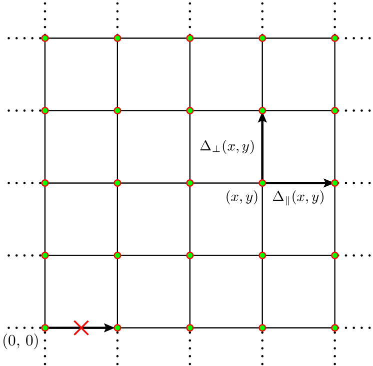
To calculate the current-redistribution factors $\Delta_{ij,mn}$, we can, without loss of generality, fix the failing bond $m$–$n$ to $m=(0,0)$ and $n=(1,0)$, see Fig. 1, and denote the $\Delta_{ij,mn}$-values as $\Delta_{\parallel}(x,y)$ if $i$–$j$ is parallel to $m$–$n$, i.e., $i=(x,y)$ and $j=(x+1,y)$, or by $\Delta_{\perp}(x,y)$ for $i=(x,y)$ and $j=x,y+1$. Introducing polar coordinates

$$d=\sqrt{x^{2}+y^{2}}\,,\quad\varphi=\arctan(y/x)\,,$$ (15)

Eqs. (14) and (7) then lead to asymptotic expressions

$$\Delta_{\parallel}(d,\varphi)\simeq\frac{-1}{\pi d^{2}}\,\cos 2\varphi$$ (16a)

and

$$\Delta_{\perp}(d,\varphi)\simeq-\frac{1}{\pi d^{2}}\,\sin 2\varphi+\dots\ .$$ (16b)

In addition to the asymptotic form of Eq. (14), Cserti Cserti2000 also derived some recursion relations, from which one can, in principle, calculate the $R(x,y)$-values exactly for arbitrary nodes $x$ and $y$. A table of exact $R(x,y)$-values for $0\leq x,y\leq 20$ has been compiled by S. and R. Hollos Hollos2005_Ref3 . Using these values, Eq. (7) then allows us to calculate exact values for $\Delta_{\parallel}(x,y)$ and $\Delta_{\perp}(x,y)$. A few examples are given in Appendix B, Table 2, and we also note that the recursion relations of Ref. Cserti2000 lead to the general result

$$\Delta_{\parallel}(x,x)=0\,.$$ (17)

A comparison of exact and asymptotic values, Eq. (16a), for $|\Delta_{\parallel}|(0,y)$ is shown in Fig. 2. It can be seen that the difference between the exact and asymptotic values is smaller than $1\%$ if $y>10$.

Figure 2: Infinite 2d square lattice: Comparison of exact values for $|\Delta_{\parallel}|(0,y)$ with their asymptotic approximations, $\delta|\Delta_{\parallel}|=\left[|\Delta_{\parallel}|^{\mathrm{exact}}-|\Delta_{\parallel}|^{\mathrm{asymp}}\right]/|\Delta_{\parallel}|^{\mathrm{exact}}$.

III.2.2 Statistics of $|\Delta|$-Values

Motivated by our analysis of stochastic load-redistribution models for cascading failure propagation Lehmann2010 , we are also interested in the overall statistics of the $|\Delta|$-values. To determine the corresponding distribution function, we use a continuum approximation similar to that developed in Ref. Lehmann2010a . We assume that the failed element is located in the center of a circular ring with an inner radius of $d_{\mathrm{min}}$ and and outer radius of $d_{\mathrm{max}}$. Assuming that the elements affected by the failure are uniformly distributed in this circular ring, and using the asymptotic approximations of Eqs. (16a) and (16b), respectively, for $|\Delta_{\parallel}|$ and $|\Delta_{\perp}|$, the probability distribution function for $|\Delta|$ can then be expressed in the form

$$\varrho(|\Delta|)=\frac{8}{\pi(d_{\mathrm{max}}^{2}-d_{\mathrm{min}}^{2})}\int\limits_{d_{\mathrm{min}}}^{d_{\mathrm{max}}}\!\!\!\mathrm{d}\xi\xi\!\!\int\limits_{0}^{\pi/2}\!\!\mathrm{d}\varphi\,\delta\left(\frac{\cos 2\varphi}{\pi\xi^{2}}-|\Delta|\right)\,,$$ (18)

where we note that to account for both $|\Delta_{\parallel}|$ and $|\Delta_{\perp}|$, an extra factor of $2$ has been included in the prefactor.

Carrying out the the integrations in Eq. (18), we obtain

$$\varrho(|\Delta|)=\frac{2}{\pi^{2}(d_{\mathrm{max}}^{2}-d_{\mathrm{min}}^{2})|\Delta|^{2}}\bigg{[}\sqrt{\smash[b]{1-\pi^{2}d_{\mathrm{min}}^{4}|\Delta|^{2}}}\\ -\sqrt{1-\pi^{2}\tilde{d}_{\mathrm{max}}^{4}|\Delta|^{2}}\bigg{]}\,,$$ (19)

where in order to account for the $\delta$-function contraint in the $\varphi$-integration, we have introduced the modified outer radius $\tilde{d}_{\mathrm{max}}=\min(d_{\mathrm{max}},1/\sqrt{\pi\Delta})$.

As we assume that the continum approximation refers to a square lattice of identical resistors with lattice constant equal to one, we set $d_{\mathrm{min}}=1$ and determine $d_{\mathrm{max}}$ by the requirement

$$\pi(d_{\mathrm{max}}^{2}-d_{\mathrm{min}}^{2})=N\,,$$ (20)

where $N$ denotes the number of resistors (bonds) in the circular ring between $d_{\mathrm{min}}$ and $d_{\mathrm{max}}$. We thus have

$$d_{\mathrm{max}}=\sqrt{\frac{N}{\pi}+1}$$ (21)

and consequently

$$\tilde{d}_{\mathrm{max}}=\min\left(\frac{1}{\sqrt{\pi|\Delta|}},\sqrt{\frac{N}{\pi}+1}\right)\,.$$ (22)

Inserting Eqs. (21) and (22) into Eq. (19), we obtain (note that $d_{\mathrm{min}}=1$)

$$\varrho(|\Delta|)=\frac{2}{\pi^{2}N|\Delta|^{2}}\begin{cases}\sqrt{1-\pi^{2}|\Delta|^{2}}-\sqrt{1-\pi^{2}(1+N/\pi)^{2}|\Delta|^{2}}&,\quad\displaystyle N|\Delta|\leq\frac{1}{1+\pi/N}\\ \sqrt{1-\pi^{2}|\Delta|^{2}}&,\quad\displaystyle\frac{1}{1+\pi/N}\leq N|\Delta|\leq\frac{N}{\pi}\,.\end{cases}$$ (23)

In order to be able to perform the limit $N\to\infty$ in a meaningful way, we introduce the scaled variable

$$\hat{\Delta}=N|\Delta|$$ (24)

In the limit $N\to\infty$, the probability density for $\hat{\Delta}$ then becomes a power law with a regularization below $\hat{\Delta}=1$

$$\varrho(\hat{\Delta})=\frac{2}{\pi\hat{\Delta}^{2}}\begin{cases}0&\hat{\Delta}\leq 0\\ 1-\sqrt{1-\hat{\Delta}^{2}}&0<\hat{\Delta}\leq 1\\ 1&\hat{\Delta}>1\\ \end{cases}$$ (25)

and the corresponding cumulative distribution function has the form

$$\mathrm{cdf}(\hat{\Delta})=\frac{2}{\pi}\begin{cases}0&\hat{\Delta}\leq 0\\ \displaystyle\arcsin\hat{\Delta}-\frac{1-\sqrt{1-\hat{\Delta}^{2}}}{\hat{\Delta}}&0<\hat{\Delta}\leq 1\\ \displaystyle\frac{\pi}{2}-\frac{1}{\hat{\Delta}}&\hat{\Delta}>1\end{cases}$$ (26)

From Eq. (23), we can further calculate the mean value $\langle|\Delta|\rangle$, and we obtain

$$\langle|\Delta|\rangle\simeq\frac{2}{\pi}\frac{\ln N}{N},\quad N\to\infty\,.$$ (27)

for asymptotically large $N$.

Finally, we can also consider the scaling of $|\Delta|$ with the distance $d$ from the failed resistor. The form of Eqs. (16a) and (16b) motivates a consideration of the quantity

$$\tilde{\Delta}=\pi d^{2}|\Delta|\,$$ (28)

and we find that this random variable is distributed according to the density

$$\varrho(\tilde{\Delta})=\begin{cases}\displaystyle\frac{2}{\pi\sqrt{1-\tilde{\Delta}^{2}}}&0\leq\tilde{\Delta}\leq 1\\ 0&\text{otherwise.}\end{cases}$$ (29)

The corresponding cumulative distribution function is then given by

$$\mathrm{cdf}(\tilde{\Delta})=\frac{2}{\pi}\arcsin\tilde{\Delta}\,,$$ (30)

where $\tilde{\Delta}$ varies in the range $0\leq\tilde{\Delta}\leq 1$.

III.2.3 Numerical Results for Finite-Size Square Lattices

We have compared the above analytical results, in particular Eqs. (16b), (26) and (30), with numerical results for a finite-size square lattice of dimensions $96\times 96$ sites connected by $18^{\prime}432$ bonds, where we have assumed periodic boundary conditions in both $x$- and $y$-direction.

Figure 3: Current-redistribution factors in a 2d square lattice consisting of $96\times 96$ sites and assuming periodic boundary conditions. The failing bond is oriented horizontally in the center of the graph, i.e. connects sites $(0,0)$ and $(1,0)$. The left (right) panel shows the current-redistribution factors in bonds parallel, $\Delta_{\parallel}$, (perpendicular, $\Delta_{\perp}$) to the failing bond. Regions of positive and negative $\Delta$ are indicated.

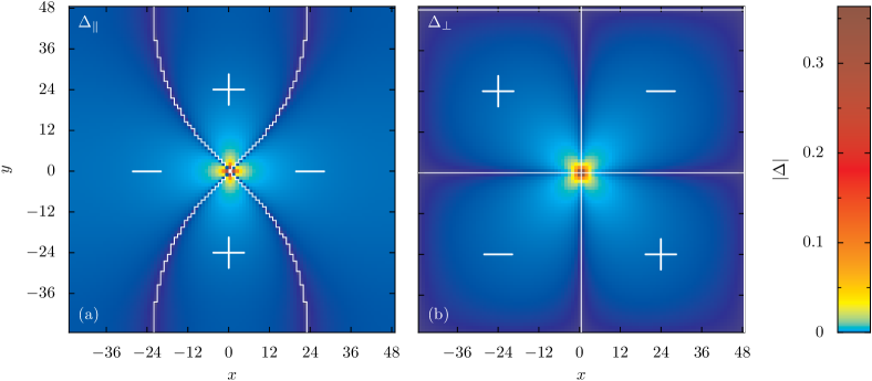
Figure 3 shows the dependence of the current-redistribution factors on orientation and position with respect to the failing bond. In the vicinity of the failing bond, we observe that (as for the infinitely large grid [cf. Eq. (17)]) the current-redistribution factors $\Delta_{\parallel}$ for bonds parallel to the failing bond vanish along the diagonals. For larger distances from the failing bond, we observe finite-size effects which lead to a deviation from this behavior. It can be shown that the deviations are due to the fact that the current flows at the boundaries of the finite-size square lattice differ considerably from those in an infinite square lattice. We also note that the form of the deviations observed in Fig. 3(a) depends strongly on the chosen boundary conditions (e.g., periodic vs. free boundary conditions).

Figure 4: Cumulative distribution function of the size-scaled magnitude of the current-redistribution factors $\hat{\Delta}=N|\Delta|$ for a 2d square lattice of $96\times 96$ sites assuming periodic boundary conditions. Dotted (red) line: result for all bonds. Dashed (blue) line: only bonds within a distance $d\leq 24$ of the failing bond. The analytical result (26) for an infinitely large system within a continuum approximation is indicated by the solid line. The inset shows the tail of the distribution function for large $\hat{\Delta}$. Crosses (red): all bonds. Squares (blue): only bonds within a distance $d\leq 24$ of the failing bond

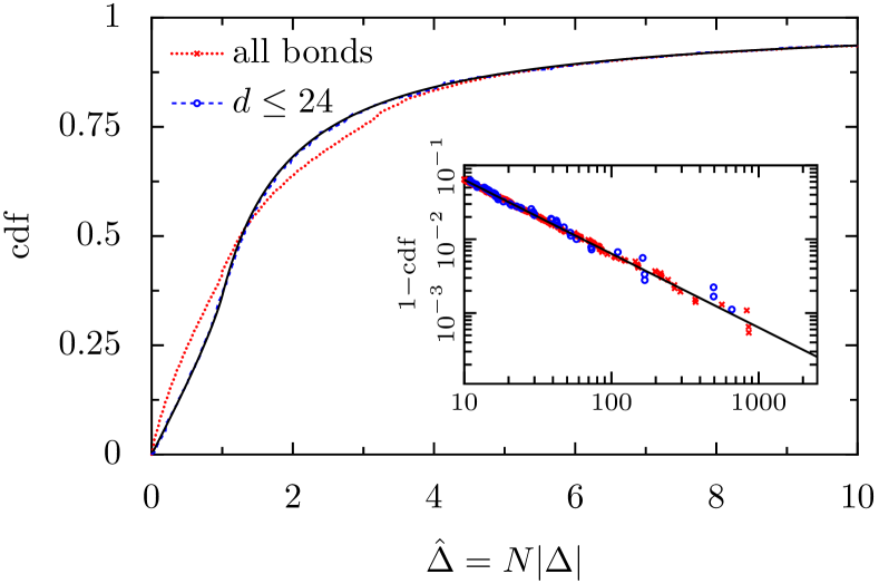
Finite-size effects can also be observed in the statistics of the current-redistribution factors. In Fig. 4, we plot the empirical cumulative distribution function of the size-scaled magnitude of the current-redistribution factors $\hat{\Delta}=N|\Delta|$ [Eq. (24)]. When comparing with the analytical result (26) for the case of an infinitely large system within a continuum approximation (solid line), we find a very good agreement if we restrict the statistics to the bonds within a distance $d\leq 24$ (blue circles) to the failed bond. Otherwise, deviations for very small $|\Delta|=\mathcal{O}(1/N)$ can be observed. For the upper tail of the distribution function shown in the inset, i.e., for the large $|\Delta|$ values of the order $1$, such deviations cannot be found.

Figure 5: Cumulative distribution function of the distance-scaled magnitude of the current-redistribution factors $\tilde{\Delta}=\pi d^{2}|\Delta|$ for a 2d square lattice of $96\times 96$ sites assuming periodic boundary conditions. The meaning of the symbols is as in Fig. 4 and the solid line denotes the analytical result (30).

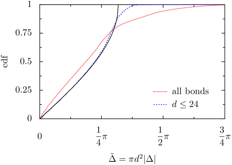
Finally, the statistics of the distance-scaled magnitude of the current-redistribution factors $\tilde{\Delta}=\pi d^{2}|\Delta|$ [Eq. (28)] is shown in Fig. 5. Here, the distance-scaling leads to a more pronounced appearance of the finite-size effects, but again the statistics of the current-redistribution factors for the bonds in the vicinity of the failed bond ($d\leq 24$) is well described by the simple analytical result of Eq. (30) from the continuum approximation (solid line).

III.3 3d Simple Cubic Lattice

For a infinite 3d simple cubic lattice of identical unit resistors, the two-point resistances $R(x,y,z)$ can be expressed in terms of the Green functions $G(x,y,z;3)$, see e.g. Ref. Cserti2000 ,

$$\begin{split}R(x,y,z)&=G(0,0,0;3)-G(x,y,z;3)\\ &=R(\infty)-G(x,y,z;3)\,.\end{split}$$ (31)

In Ref. Joyce2002 , it is shown that

$$\begin{split}R(\infty)&=\frac{1}{96\pi^{3}}(\sqrt{3}-1)\big{[}\Gamma(1/24)\Gamma(11/24)\big{]}^{2}\\ &=0.505462\dots\end{split}$$ (32)

and that $G(x,y,z;3)$ has the following asymptotic expansion,

$$\begin{split}G(x,y,z;3)\simeq\frac{1}{2\pi d}&+\frac{1}{8\pi d^{7}}\big{[}(x^{4}+y^{4}+x^{4})\\ &-3(x^{2}y^{2}+x^{2}z^{2}+y^{2}z^{2})\big{]}\end{split}$$ (33)

for $d=\sqrt{x^{2}+y^{2}+z^{2}}\to\infty$.

We now consider the removal of bond $m$–$n$, where $m=(0,0,0)$ and $n=(0,0,1)$. The current-redistribution factors $\Delta_{\parallel}^{(z)}(x,y,z)$ for affected bonds parallel to the $z$-axis can then be expressed as [see Eq. (7)]

$$\Delta_{\parallel}^{(z)}(x,y,z)=\frac{R(x,y,z+1)+R(x,y,z-1)-2R(x,y,z)}{2[1-R(0,0,1)]}\,.$$ (34)

Using Eq. (33) and $R(0,0,1)=1/3$, we then obtain

$$\begin{split}\Delta_{\parallel}^{(z)}(x,y,z)&{}\simeq\frac{3}{8\pi d^{3}}[1-3(z/d)^{2}]\\ &=\frac{3}{8\pi d^{3}}[1-3\cos^{2}\theta]\end{split}$$ (35a)

for $$d=\sqrt{x^{2}+y^{2}+z^{2}}\to\infty \theta z (x,y,z)$$, where denotes the angle between the -axis and the vector .

Similarly, for affected bonds parallel to the $x$-($y$-)axis, we obtain

$$\Delta_{\perp}^{(z)}(x,y,z)\simeq-\frac{9}{16\pi d^{3}}\sin 2\theta\cos\varphi\,,$$ (35b)

where $\varphi$ refers to the angle between the $x$-($y$-)axis and the vector $(x,y,0)$, respectively.

Apart from the angular dependences, the dominating asymptotic behavior of $|\Delta|$ is thus given by

$$|\Delta|\simeq\frac{1}{d^{3}}\,$$ (36)

compared with the $1/d^{2}$ behavior of $|\Delta|$ for a 2d square lattice [cf. Eqs. (16a) and (16b)].

Using the same continuum approximation as in Sec. III.2, we can show that the dominating behavior of the distribution function $\varrho(|\Delta|)$ is given by the power law

$$\varrho(|\Delta|)\simeq\frac{1}{|\Delta|^{2}}\,.$$ (37)

Note that this behavior is identical to that of 2d regular lattices, see Eq. (25), and we expect that this is also valid for all regular lattices of dimension four and higher. For quasi-one-dimensional lattices, as well as for small world networks, however, the behavior of $|\Delta|(d)$ and of $\varrho(|\Delta|)$ is completely different, as we shall see in the following sections.

IV Quasi-One-Dimensional Networks

For a strictly one-dimensional system (1d chain) with free boundary conditions, every bond removal leads to a separation of the network into two unconnected parts, so that the current-redistribution factors are not defined.

We can, however, consider quasi-one-dimensional systems such as, e.g., the semi-infinite ladder shown in Fig. 6. Here, we have assumed unit conductances, $g=1$, along the ladder as well as for the leftmost spoke and equal conductances $g$ for all other spokes.

Figure 6: Semi-infinite ladder consisting of bonds with unit conductances along the ladder as well as for the leftmost spoke (solid line), which is assumed to fail, and equal conductances $g$ of the other spokes (dashed line).

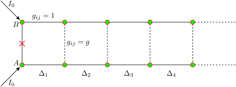
We then restrict ourselves to a failure of the leftmost spoke and consider the current-redistribution factors $\Delta_{n}$ in an infinite (one-sided) ladder for the bonds along the ladder (see Fig. 6). An analytical calculation of the current-redistribution factors $\Delta_{n}$ is straightforward and leads to the result

$$\Delta_{n}=X(g)^{-(n-1)}\,$$ (38)

where

$$X(g)=\frac{G+g}{G}=\frac{\sqrt{g^{2}+2g}+g}{\sqrt{g^{2}+2g}-g}\,.$$ (39)

The current-redistribution factors $\Delta_{n}$ thus depend exponentially on the distance $d=n$ from the removed bond. The slope $s(g)$ of the linear relation $\ln\Delta_{n}$ vs. $n$ is given by

$$s(g)=\ln X(g)\,.$$ (40)

For $g\to 0$, this slope becomes $s(g)\approx\sqrt{2g}$, and in the case where all conductances are equal, i.e., $g=1$, we have

$$s(1)=\ln\left(\frac{\sqrt{3}+1}{\sqrt{3}-1}\right)\,.$$ (41)

V Ring topologies with Long-Range Connections

A particulary interesting class of networks can be obtained when random long-range links are added to originally regular structures such as the ones studied in the previous sections. In a seminal paper Watts1998 , Watts and Strogatz found that when only a small fraction of bonds in a ring lattice are randomly rewired, the average shortest path length drops significantly and reaches values like in a completely random graph. The local structure, however, is retained. Watts and Strogatz argued that such a semi-random model captures crucial properties of many real world graphs including, e.g., power grids. Additionally, by the nature of their construction, such networks (and their generalization to higher dimensions) maintain the underlying spatial structure including its (Euclidean) metric Barthelemy2011 . In the context of our investigations, this will allow us to study the distance dependence of the current redistribution also for non-regular networks that represent more realistic models for infrastructure networks. We further note that our statistical approach is a particularly adequate method to study current redistribution in this type of networks, as they are random by construction. Care has to be taken, however, that now in addition to the statistics of the affected bonds, the disorder statistics of the network itself has to be considered.

In this Section, we will first consider the behavior of the current redistribution in the case of a randomly placed single long-range connection in a ring. As a second extreme case we will then look at a ring with additional connections added between each non-neighbouring pair of nodes, i.e. a completely connected graph. Finally, we will present extensive numerical calculations for the current redistribution in a variant of the Watts-Strogatz model where, instead of rewiring connections, additional long-range shortcuts are randomly added Newman1999a .

V.1 Ring with a Single Long-Range Connection

The case of a ring with a single long-range connection can be treated analytically. Consider the graph shown in Fig. 7 and assume that a bond in the segment with $k$ links fails. Then the current-redistribution factors only assume two different values: $|\Delta|=1$ if the considered bond is in the same segment as the failed bond, and $|\Delta|=1/(N-k+1)$ if it is in the other segment. If a bond in the segment with $N-k$ links fails, the two values are $|\Delta|=1$ and $|\Delta|=1/(k+1)$.

Figure 7: Ring with one long-range connection.

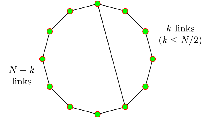
Using a straightforward counting procedure, we can easily determine the frequencies with which the three $|\Delta|$-values occur when we vary the position of the failed bond. From these we can then calculate the average of $|\Delta|(d)$ with respect to all possible positions of the failed bond, $\langle|\Delta|\rangle(d,k;N)$, where $d$ refers to the distance (measured along the ring) between the considered and the failed bond, $k$ is explained in Fig. 7, and $N$ is the size of the ring (number of sites).

In the limit as $N\to\infty$, we can introduce the normalized variables $\delta=d/N$ and $\kappa=k/N$, where $\delta$ and $\kappa$ can be considered as continuous ($0\leq\delta,\kappa\leq 1/2$). It follows that in this limit, $\langle|\Delta|\rangle$ can be written as

$$\langle|\Delta|\rangle(\delta,\kappa)=\begin{cases}\displaystyle 1-2\delta\,,&0\leq\delta\leq\kappa\\ \displaystyle 1-2\kappa\,,&\kappa\leq\delta\leq 1/2\,,\end{cases}$$ (42)

and its average over all normalized lengths $\kappa$ of the long-range links becomes

$$\langle\!\langle|\Delta|\rangle\!\rangle(\delta)=1-2\delta+2\delta^{2}\,,\quad 0\leq\delta\leq 1/2\,.$$ (43)

Another quantity of interest that can be calculated analytically in the limit as $N\to\infty$, is the graph-distance $\tilde{\delta}$ between two points on the ring. The calculations are again straightforward but somewhat more tedious than for $|\Delta|$, as we have to consider considerably more sub-cases. The final result is

$$\langle\tilde{\delta}\rangle(\delta,\kappa)=\begin{cases}\delta-\kappa\delta+\kappa^{2}/2\,&0\leq\kappa\leq 2\delta\\ \delta\,&2\delta\leq\kappa\leq 1/2\end{cases}$$ (44a)

if $$0\leq\delta\leq 1/4$$ and

$$\langle\tilde{\delta}\rangle(\delta,\kappa)=\begin{cases}\delta-\kappa\delta+\kappa^{2}/2\,&0\leq\kappa\leq 1-2\delta\\ 1/2-\kappa+\kappa^{2}\,&1-2\delta\leq\kappa\leq 1/2\end{cases}$$ (44b)

if $1/4\leq\delta\leq 1/2$. The average over all lengths $\kappa$ of the the long-range link finally becomes

$$\langle\!\langle\tilde{\delta}\rangle\!\rangle=\delta-\frac{4}{3}\,\delta^{3}\,.$$ (45)

Figure 8: Behavior of (a) $\langle\!\langle\tilde{\delta}\rangle\!\rangle$ [Eq. (45)] and (b) $\ln\langle\!\langle|\Delta|\rangle\!\rangle$ [Eq. (43)] vs. $\delta$.

It is interesting to note the similarity in the behavior of $\langle\!\langle\tilde{\delta}\rangle\!\rangle$ and $\ln\langle\!\langle|\Delta|\rangle\!\rangle$ (see Fig. 8). Both quantities start out linearly for $0\leq\delta\approx 0.2$ and then saturate as $\delta\to 0.5$. This suggests that we have the following approximate relation between $\langle\!\langle|\Delta|\rangle\!\rangle$ and $\langle\!\langle\tilde{\delta}\rangle\!\rangle$:

$$\langle\!\langle|\Delta|\rangle\!\rangle\approx\mathrm{e}^{-\lambda\langle\!\langle\tilde{\delta}\rangle\!\rangle}\,.$$ (46)

As in quasi-one-dimensional networks (Sec. IV), we thus observe at least an approximate exponential dependence of the current-redistribution factors $|\Delta|$ on the distance between the considered and the failed bond, but here only in an average sense and on if we replace the Euclidean distance along the ring by the graph distance.

The relation of Eq. (46) is surprisingly accurate if we set $\lambda\approx 2$. The value $\lambda=2$ is obtained if we require that the exact and approximate expressions for $\langle\!\langle|\Delta|\rangle\!\rangle$, Eqs. (43) and (46), respectively, have equal initial slopes (at $\delta=0$). If, on the other hand, we require that Eq. (46) reproduces the exact value of $\langle\!\langle|\Delta|\rangle\!\rangle=1/2$ at $\delta=1/2$, then $\lambda=3\ln 2=2.079$, which appears to give an even superior approximation.

V.2 Fully Connected Ring

We now consider the opposite extreme of complete connectivity, i.e., each site on the ring is connected to every other site.

If all connections have the same conductance, $g_{ij}=1$, it can be shown that

$$\begin{split}R_{ij}&=\frac{2}{N}\quad\text{for all $i\neq j$}\,,\\ R_{ii}&=0\end{split}$$ (47)

This leads to

$$|\Delta_{ij,mn}|=\begin{cases}\displaystyle\frac{1}{N-2}&\text{if bond $i$--$j$ is adjacent to $n$--$m$}\\ 0&\text{otherwise.}\end{cases}$$ (48)

The average value of $|\Delta|$ thus becomes

$$\langle|\Delta|\rangle=\frac{2}{(N-1)(N-2)}\simeq\frac{2}{N^{2}}\quad(N\to\infty)\,.$$ (49)

If the long-range links have smaller conductances than the nearest neighbor links on the ring, i.e., $g^{\mathrm{longrange}}_{ij}=g<1$, we are no longer able to determine the $|\Delta_{ij,mn}|$-values analytically. Numerical simulations, however, show unambigously that $|\Delta(d)|$ decreases exponentially with the distance $d$ (measured along the ring) from the failed link,

$$|\Delta(d)|\approx\mathrm{e}^{-s(g,N)d}$$ (50)

with an exponent $s(g,N)$ that approaches the value

$$s(g,N)\approx\sqrt{Ng}\quad\text{if $Ng\ll 1$}\,.$$ (51)

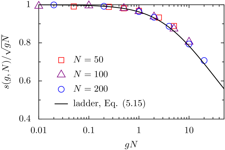
For the fully connected ring with long-range conductances $g<1$, $|\Delta(d)|$ thus exhibits quasi-one-dimensional behavior, and this observation can even be further quantified: It turns out that in the limit of large $N$, a fully connected ring is very accurately approximated by a one-dimensional ladder of size $N/2$ with spoke conductances $g^{\text{spoke}}=gN/2$, if $g\ll 1$, i.e. [see Eqs. (39) and (40)],

$$s(g,N)\approx\ln\frac{\sqrt{g^{2}+4g/N}+g}{\sqrt{g^{2}+4g/N}-g}\,,\quad\text{if $g\ll 1$ and $N\gg 1$}\,.$$ (52)

The accuracy of the approximation (52) is demonstrated by the numerical results shown in Fig. 9.

Figure 9: Behavior of $s(g,N)$, the exponent that characterizes the decrease of $|\Delta(d)|$ in a fully connected ring of size $N$ with long-range conductances $g$. Comparison is made with the corresponding exponent of a one-dimensional ladder with spoke-conductances $gN/2$, see Eq. (52).

V.3 Random Small-World Networks

Finally, we turn our attention to the case of random small-world networks, which we construct from a (one-dimensional) ring by adding random shortcuts similar to the model by Newman and Watts in Ref. Newman1999a . Specifically we start from a ring of $N$ sites with each site initially being connected to its two nearest neighbors and then add long-range connections randomly with probability $2p/N$ between the $N(N-3)/2$ different pairs of non-nearest neighbours, so that the average number of long-range links is $p(N-3)\simeq pN$ for large $N$ .

To investigate the behavior of $\Delta_{ij,mn}$ in these small-world networks, we have performed a large number of simulations on networks of varying sizes (up to $N=10000$) and for different values of $p$ ($0.001\leq p\leq 1$). A selection of corresponding results is shown in Figs. 10–12.

Figure 10: Averaged $|\Delta|$ as a function of the scaled ring distance $pd$ for rings of size $N=4000$ (red, open symbols) and $10000$ (blue, closed symbols), and for different values of the probability parameter $p$. The numerical results represent averages over both the location of the failing bond and $25$ realizations of the small-world network. The lines serve as a guide to the eye. The arrows indicate the location of the critical ring distances $d_{0}(p,N)$ [Eq. (55)]

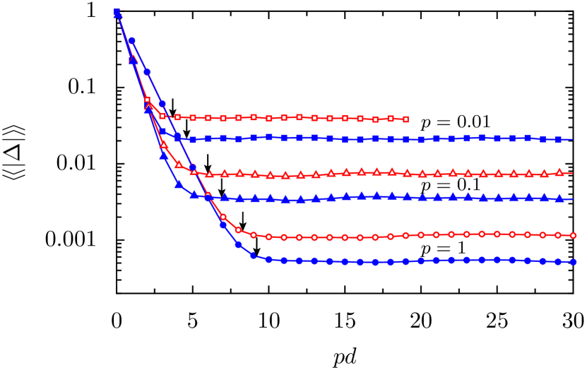
Figure 10 refers to the behavior of $\langle\!\langle|\Delta|\rangle\!\rangle$ as a function of the scaled ring distance $pd$. The average $\langle\!\langle|\Delta|\rangle\!\rangle$ is an average over 25 different realizations of the corresponding random network as well as an average over all locations of the failed bond and the corresponding (two) affected connections at the given distance. We note that failures and their effects are only considered for bonds on the ring. We observe that the behavior of $\langle\!\langle|\Delta|\rangle\!\rangle$ vs. $pd$ is distinctly different from that of regular networks: For small values of $pd$, $\langle\!\langle|\Delta|\rangle\!\rangle$ initially decreases exponentially with $d$,

$$\langle\!\langle|\Delta|\rangle\!\rangle\approx\exp(-\lambda pd)\,,$$ (53)

i.e., the network behaves like a quasi-one-dimensional system. Around some critical value of $d$, $d=d_{\mathrm{c}}(p,N)$, however, $\langle\!\langle|\Delta|\rangle\!\rangle$ exhibits a transition and stays constant for larger values of $pd$,

$$\langle\!\langle|\Delta|\rangle\!\rangle\approx\Delta_{0}(p,N)\quad\text{if $d\gtrsim d_{\mathrm{c}}(p,N)$.}$$ (54)

Interestingly, the behavior of $-\ln\langle\!\langle|\Delta|\rangle\!\rangle$ vs. $d$ is remarkably similar to that of the graph distance (shortest-path length) in a small-world network Menezes2000 ,

$$d_{\mathrm{graph}}\approx\begin{cases}\displaystyle d&\text{if $d\lesssim d_{0}=\ln(pN)/p$}\\ d_{0}&\text{if $d\gtrsim d_{0}$}\end{cases}\,,$$ (55)

and we note that the critical distance $pd_{\mathrm{c}}(p,N)$ above which $\langle\!\langle|\Delta|\rangle\!\rangle$ saturates coincides quite well with the critical value $pd_{0}=\ln(pN)$ in Eq. (55), see Fig. 10. From the above observations and considerations, we may be tempted to express $\langle\!\langle|\Delta|\rangle\!\rangle$ as

$$\langle\!\langle|\Delta|\rangle\!\rangle\approx\exp(-\lambda pd_{\mathrm{graph}})\,.$$ (56)

It then turns out that this relation yields a very accurate description of the plateaus $\Delta_{0}(p,N)$ if we set $\lambda=0.825$,

$$\Delta_{0}(p,N)\approx\exp(-0.825pd_{0})=(pN)^{-0.825},$$ (57)

see Table 1.

			$\log_{10}(\Delta_{0})$
$p$	$N$	$pN$	Simulation	Eq. (57)	Eq.(62b)
$0.01$	$4000$	$40$	$-1.40$	$-1.32$	$-1.23$
$0.01$	$10000$	$100$	$-1.67$	$-1.65$	$-1.53$
$0.1$	$4000$	$400$	$-2.13$	$-2.15$	$-2.08$
$0.1$	$10000$	$1000$	$-2.45$	$-2.48$	$-2.36$
$1$	$4000$	$4000$	$-2.95$	$-2.97$	$-2.88$
$1$	$10000$	$10000$	$-3.28$	$-3.30$	$-3.23$

Table 1: Comparison of the observed plateau values $\Delta_{0}(p,N)$ with two analytical expressions, Eq. (57) and Eq. (62b), see text.

In this context, it may be worth noting that Korniss et al. Korniss2006 have derived an asymptotic expression for the two-point resistance in small-world networks in the limit $N\to\infty$,

$$\langle\!\langle R(d)\rangle\!\rangle\simeq 1-\exp(-\sigma d)\,,$$ (58)

and an analysis of their numerical results shows that these can be very accucurately described by $\sigma=0.825p$.

For small values of $d_{\mathrm{graph}}$, however, where $d_{\mathrm{graph}}=d$, expression (56) only approximates the observed behavior of $\langle\!\langle|\Delta|\rangle\!\rangle$ if we assume that $\lambda$ becomes $p$-dependent. From our numerical simulation (see, e.g., Fig. 10), we observe that $\ln\langle\!\langle|\Delta|\rangle\!\rangle$ vs. $pd$ exhibits an initial slope $\lambda(p)\approx 1.4$ if $p\lessapprox 0.1$, $\lambda(p{=}0.2)\approx 1.28$, $\lambda(p{=}0.5)\approx 1.11$, and $\lambda(p{=}1)\approx 0.93$. We also note that $\lambda(p)$ appears to be independent of system size $N$, but the observed $p$-dependence of $\lambda(p)$ does not seem to have an obvious explanation.

In addition to the dependence of $\langle\!\langle|\Delta|\rangle\!\rangle$ on the distance $d$ between affected and failed bond, we have also analyzed the overall statistics of the $|\Delta|$-values. Corresponding numerical results are shown in Figs. 11 and 12.

Figure 11: Average $\langle\!\langle|\Delta|\rangle\!\rangle$ of the current-redistribution factors $|\Delta_{ij,mn}|$ for rings of different size $N$ and for different probabilities $p$ of adding long-range connections. The numerical results represent averages over both the location of the failing bond and $25$ realizations of the small-world network. The line marked “Lorentz” corresponds to the approximation of Eq. (61) for $\langle|\Delta|\rangle$ vs. $pN$.

Figure 12: Cumulative distribution function of the scaled current-redistribution factors, $Np\langle|\Delta|\rangle$, for a ring with $N=10000$ sizes and different $p$-values for two different realizations of the random long-range links (solid and dashed lines). The dotted curve denoted by “Lorentz” corresponds to Eq. (60)

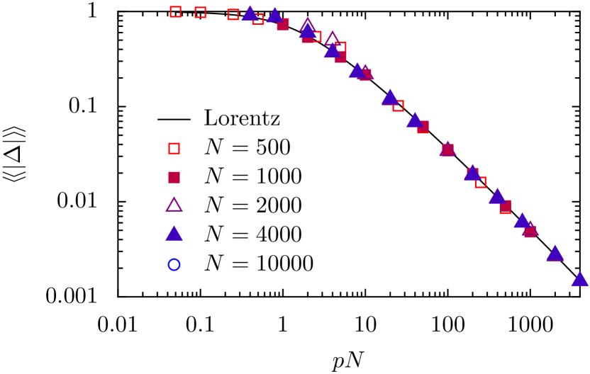
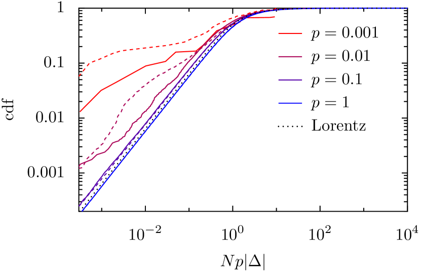
A detailed analysis of these numerical results has shown that many of the observed features can be described if we assume that the statistics of $pN|\Delta|$-values is a half-Lorentz distribution (of width $\gamma=1$) with a cutoff at $|\Delta|=1$ and a $\delta$-function at $|\Delta|=1$, i.e.

$$\varrho(y)=\frac{2}{\pi}\,\frac{1}{1+y^{2}}+\bigg{[}1-\frac{2}{\pi}\arctan(pN)\bigg{]}\,\delta(y-pN)\quad(y\geq 0)$$ (59)

where $y=pN|\Delta|$. The corresponding cumulative distribution function is given by

$$\mathrm{cdf}(|\Delta|)=\frac{2}{\pi}\arctan(pN|\Delta|)\quad(0\leq|\Delta|\leq 1)$$ (60)

and the mean value of $|\Delta|$ is

$$\langle|\Delta|\rangle=\frac{1}{\pi}\,\frac{1}{pN}\ln\big{[}1+(pN)^{2}\big{]}+1-\frac{2}{\pi}\arctan(pN)$$ (61)

which has the following limits:

$$\langle|\Delta|\rangle\simeq 1-\frac{1}{\pi}\,pN\,,\quad pN\to 0$$ (62a)

and

$$\langle|\Delta|\rangle\simeq\frac{2}{\pi}\,\frac{\ln(pN)}{pN}\,,\quad pN\to\infty\,.$$ (62b)

From Fig. 11, we see that Eq.(61) gives a remarkably accurate description of the empirical $\langle\!\langle|\Delta|\rangle\!\rangle$ vs. $pN$ behavior over a large range of $N$ and $p$ values.

For a comparison of the expression of Eq. (60) for the cumulative distribution function, we consider only $|\Delta|$-values for fixed realizations of the random network. Then, Eq. (60) only appears to be a reasonably accurate approximation of the numerical results if $p$ is not too small (see Fig. 12). Additional numerical simulations for $N=100$, $1000$ and $2000$, indeed show a nice collapse of the data on the curve described by Eq. (60) if $pN$ is larger than about $100$. A value of $pN\geq 100$ implies that the mean vertex-to-vertex distance is smaller than about $1/10$ of the mean distance along the ring, see e.g. Fig. 5 of Ref. Newman1999a . According to the discussion in Ref. Newman1999a , this is the small-world regime, which suggests that the Lorentz distribution of Eq. (60) is a good approximation of the $|\Delta|$-statistics only if the network exhibits small-world behavior. For very small values of $pN$, we reach the limiting case of only a few long-range connections and the result, thus, depends on the specific location of these connections. For larger values of $pN$, however, the $|\Delta|$-distribution becomes independent of the specific realization of the network and the system shows self-averaging behavior. Our numerical results indicate that this self averaging is connected to the small-world regime.

On the other hand, for very large $pN$-values, of the order of $N^{2}$, we expect that the cdf-behavior will approach the degenerate one of a fully connected ring (see Subsection V.2). Preliminary simulations confirm this trend, but they are very time-consuming and we cannot yet give a quantitative description of the transition from the Lorentz-behavior to the behavior of a fully connected ring.

Finally, we note that Eq. (62b) not only gives a very accurate description of the observed $\langle\!\langle|\Delta|\rangle\!\rangle$ vs. $pN$ behavior (Fig. 11), but can also be used to describe the $pN$-dependence of the $\langle\!\langle\Delta\!\rangle\!\rangle$-plateaus in Fig. 10. As Eq. (62b) refers to the mean value $\langle|\Delta|\rangle$, it naturally overestimates the plateau values (see Table 1), but it can also be seen that the overestimation decreases with increasing $pN$. This reflects the fact that with increasing $pN$, the width of the plateau region (compared to the region of exponential decay) becomes more and more dominant. We also note, however, that the Lorentz-approximation gives no information on the (exponential) behavior of $\langle\!\langle|\Delta|\rangle\!\rangle$ vs. $pd$ for small $pd$-values.

VI Summary and Conclusions

In this paper, we have studied the current redistribution in resistor networks after the failure of a current-carrying bond. The corresponding current-redistribution factors $\Delta_{ij,mn}$ characterize in a convenient way the vulnerability of a flow-carrying network with respect to cascading failures Lehmann2010 .

Information on a network’s vulnerability, in the sense of identifying the most vulnerable links (links with largest voltage drops) can also be obtained from relations between two nodes, e.g., from the two-point resistances $R_{ij}$ Korniss2006 . The current-redistribution factors $\Delta_{ij,mn}$, however, are relations between two edges and thus represent a more natural and more adequate tool to study the vulnerability of a network with respect to flow-induced failure cascades Schaub2014 .

An important property of the current-redistribution factors $\Delta_{ij,mn}$ is their dependence on the distance $d$ between link $i$–$j$ from the failed link $m$–$n$. In this paper, we have thus determined this dependence $\Delta(d)$ for different types of networks, and we have studied the influence of network topology (regular networks vs. small-world networks) and dimensionality on $\Delta(d)$. In addition, we have also analyzed the overall statistics of the $\Delta$-values in the different network topologies. This aspect of the present investigations was, in particular, motivated by our recent studies of stochastic load-redistribution models Lehmann2010 ; Lehmann2010a .

In Sec. II, we have outlined the calculation of the current redistribution factors $\Delta_{ij,mn}$ in a resistor network and discussed the use of an interesting relation between $\Delta_{ij,mn}$ and the two-point resistances $R_{in}$, $R_{im}$, $R_{jn}$, $R_{jm}$, and $R_{mn}$, see Eq. (7). We note that this relation is non-linear (because of $R_{mn}$ in the denominator), i.e., average values of $\Delta_{ij,mn}$ cannot be expressed in terms of average two-point resistances.

In Sec. III, we have calculated the $\Delta$-values for resistor networks that have the topology of regular lattices (one-dimensional chain, two-dimensional square lattice, and three-dimensional simple cubic lattice). As the one-dimensional chain is a degenerate case, i.e., the $\Delta$-values depend on the boundary conditions or are even not properly defined, we have also considered quasi-one-dimensional networks (one-dimensional ladders), for which these problems do not appear, see Sec. IV.

For all regular networks, we have derived exact analytic expressions for $\Delta(d)$, where $d$ denotes the distance of the considered link from the failed link. It turns out that the behavior of $\Delta(d)$ in a quasi-one-dimensional ladder is completely different from that in higher-dimensional regular networks.

For quasi-one-dimensional lattices, $|\Delta|$ decays exponentially with increasing distance d from the failed link, $|\Delta|(d)\simeq\exp(-\chi d)$, whereas for higher dimensional lattices we observe a power law decay, $|\Delta|(d)\simeq 1/d^{2}$ for the two-dimensional square lattice and $|\Delta|(d)\simeq 1/d^{3}$ for the three-dimensional simple cubic lattice. Apart from the overall power law decay, the $|\Delta|$-behavior in regular two- and three-dimensional lattices exhibits a characteristic angular dependence. We further observe that the dominating behavior of the overall distribution function, $\varrho(|\Delta|)$, is the same for all regular lattices of dimension two and higher, $\varrho(|\Delta|)\simeq 1/|\Delta|^{2}$. We finally remark that breakdown models with a similar power-law dependence of the stress redistribution have been studied in Refs. Hidalgo2002 and Lehmann2010a . Interestingly enough, if we compare the $|\Delta|^{-2}$ load redistribution with the one of the stochastic fibre-bundle model studied in Ref. Lehmann2010a , we find that it would correspond to a range-dependent load sharing with a $r^{-2}$-dependence, which is just at the border of the transition between global and local load sharing Hidalgo2002 .

In random small-world networks the behavior of the current redistribution factors $\Delta_{ij,mn}$ becomes much more complex (Section V.3). We consider networks that are constructed from a one-dimensional ring by adding random long-range links with probability $2p/N$ (Newman and Watts, see Ref. Newman1999a ), and we have performed a large number of numerical simulations for network sizes up to $N=10’000$ sites and for $p$-values in the range $0.001<p<1$.

The behavior of the mean value of $|\Delta|$ as a function of the ring distance $d$ turns out to be distinctly different from that observed in regular networks. For small values of $pd$, $\langle\!\langle|\Delta|\rangle\!\rangle$ decreases exponentially with $d$, i.e., the behavior is similar to that of a quasi-one-dimensional network. Around some critical value, $d=d_{\mathrm{c}}(p,N)$, however, $\langle\!\langle|\Delta|\rangle\!\rangle$ saturates and stays constant for larger values of $pd$. It is interesting to note that the corresponding behavior of $-\ln\langle\!\langle|\Delta|\rangle\!\rangle$ vs. $d$ is very similar to that of the graph distance  $d_{\mathrm{graph}}$ (shortest-path distance) vs. $d$, see e.g. Ref. Newman1999a . In small-world networks, $|\Delta|$ thus appears to depend exponentially on the shortest-path distance to the failed link. Note that we have observed a similar behavior already in the limiting case of a single long-range connection, but there only if $|\Delta|$ is averaged over all possible lengths and positions of the long-range link. In random small-world networks, however, this behavior is independent of the specific realization, at least if $pN$ is not too small.

Another interesting aspect of the current redistribution in small-world networks is the overall statistics of the $|\Delta|$-values. A careful analysis of our numerical results has revealed that the observed dependences can very accurately be described by assuming that the statistics of the $pN|\Delta|$-values is given by a half-Lorentz distribution of width $\gamma=1$, Eq. (59). A detailed analysis of the cumulative distribution function $\mathop{\mathrm{missing}}{cdf}(|\Delta|)$ shows, however, that it follows a Lorentz distribution only if $pN\gtrsim 100$, i.e. if the network exhibits small-world behavior, see Fig. 12 and the corresponding remarks in the text. For smaller values of $pN$, the results for $\mathop{\mathrm{missing}}{cdf}(|\Delta|)$ depend on the specific realization of the randomly chosen long-range connections. If $pN\gtrsim 100$ (but not too close to the fully connected limit), this is no longer the case, i.e., the system shows self-averaging behavior.

These observations are very interesting in several respects. They show that the transition to a self-averaging behavior occurs at precisely the $pN$-value, above which the $|\Delta|$-distribution is described by a (half-)Lorentz distribution. The Lorentz distribution, in turn, has a fat tail, $\simeq 1/|\Delta|^{2}$, and this is a very important aspect for the onset and propagation of failure cascades. The $|\Delta|$-distributions of regular lattices in two- and three dimensions, in fact, also exhibit a $1/|\Delta|^{2}$ tail. We note, however, that in these cases this behavior of $\varrho(|\Delta|)$ is an artefact of the $d$-dependence of $|\Delta|$. In small-world networks, on the other hand, the graph-distance is the same for almost all links that are not very close to the failed link, so that here the statistics of $|\Delta|$-values is a more meaningful concept.

Small-world networks are often used as models for real-world infrastructure networks, e.g., power grids. The $|\Delta|$-statistics of such networks could thus be an adequate concept to describe the influence of a failed connection on the other connections, and we have seen that in small-world networks, this influence is almost independent of the geometrical location of the affected connections. This gives some justification to the use of stochastic models, such as proposed in Ref. Lehmann2010 , to describe cascading failure propagation in real-world networks.

The analysis of such stochastic breakdown models is, however, beyond the scope of the present paper. Interesting questions in this context would be the corresponding dependence of breakdown properties on the load-redistribution statistics. Similar investigations have been performed for local load-sharing rules in fibre-bundle models, see e.g. Refs. Sinha2015 and Kim2005 , where a transition to a mean-field behavior of the system was observed as a function of the dimensionality of the system (for regular lattices) or the rewiring probability (for small-world networks), respectively. It is an open question whether such transitions can also be observed in resistor networks, where the current-redistribution, as given by Kirchhoff’s laws, is inherently non-local.

Appendix A Derivation of Eq. (7)

In the following, we prove Eq.(7) and start by writing the solution to Eq.(4) in the form

$$U=\mathsf{X}I^{\mathrm{s}},$$ (63)

where $\mathsf{X}$ denotes the (pseudo-)inverse of the nodal admittance matrix $\mathsf{Y}$. A removal of bond $m$–$n$ can now be modeled (as far as the rest of the network is concerned) by adding suitably chosen current injections $\Delta I^{\mathrm{s}}_{m}=-\Delta I^{\mathrm{s}}_{n}$ (see, e.g., Ref. Wood1996 , Appendix 11 A). If $\Delta I^{\mathrm{s}}_{m}$ is chosen such that

$$\Delta I^{\mathrm{s}}_{m}=I^{\prime}_{mn}\,,$$ (64)

where $I^{\prime}_{mn}$ is equal to the current flow through bond $m$–$n$, there is no current flowing from nodes $m$ and $n$ to the rest of the network. As far as the rest of the network is concerned, this is the same as a removal of bond $m$–$n$.

With Eq. (63) we can now express the change of voltage $\Delta U_{k}$ in an arbitrary node $k$ in terms of the injected currents $\Delta I^{\mathrm{s}}_{m}=-\Delta I^{\mathrm{s}}_{n}$ as

$$\Delta U_{k}=(X_{km}-X_{kn})\Delta I^{\mathrm{s}}_{m}\,.$$ (65)

Using Ohm’s law, this yields, on one hand, the new current through bond $m$–$n$:

$$\begin{split}I^{\prime}_{mn}&{}=I_{mn}+\frac{\Delta U_{m}-\Delta U_{n}}{r_{mn}}\\ &{}=I_{mn}+\frac{X_{mm}+X_{nn}-2X_{mn}}{r_{mn}}\,\Delta I^{\mathrm{s}}_{m}\,.\end{split}$$ (66)

Together with condition (64), this gives an expression for the current injections in terms of the original current $I_{mn}$ through bond $m$–$n$:

$$\Delta I^{\mathrm{s}}_{m}=\frac{1}{1-(X_{mm}+X_{nn}-2X_{mn})/r_{mn}}I_{mn}\,.$$ (67)

On the other hand, we can again use Ohm’s law in the definition (3) of the current-redistribution factor

$$\Delta_{ij,mn}=\frac{I^{\prime}_{ij}-I_{ij}}{I_{mn}}=\frac{(\Delta U_{i}-\Delta U_{j})/r_{ij}}{I_{mn}}$$ (68)

and obtain, together with Eqs. (65) and (67), the result

$$\Delta_{ij,mn}=\frac{(X_{im}-X_{in}-X_{jm}+X_{jn})/r_{ij}}{1-(X_{mm}+X_{nn}-2X_{mn})/r_{mn}}\,.$$ (69)

Finally, with Eqs. (8), (9), and (63), we find

$$R_{ij}=X_{ii}+X_{jj}-2X_{ij}\,,$$ (70)

and Eq.(69) can thus be written as

$$\Delta_{ij,mn}=\frac{1}{2r_{ij}}\frac{R_{in}-R_{im}+R_{jm}-R_{jn}}{1-R_{mn}/r_{mn}}\,.$$ (71)

Appendix B Exact values of $\Delta_{\parallel}(x,y)$ and $\Delta_{\perp}(x,y)$ for an Infinite 2d Square Lattice

Using Eq. (7), we can calculate exact $\Delta(x,y)$-values from exact values for the two-point resistances $R(x,y)$. For an infinite square lattice, a table of such values [for $0\leq x,y\leq 20$] has been compiled by S. and R. Hollos Hollos2005_Ref3 . In Table 2, we list a few examples of exact expressions for $|\Delta_{\parallel}|(x,y)|$ and $|\Delta_{\perp}|(x,y)$.

$\displaystyle|\Delta_{\parallel}|(0,1)=\frac{4}{\pi}-1$	$\displaystyle|\Delta_{\perp}|(0,0)=1-\frac{2}{\pi}$
$\displaystyle|\Delta_{\parallel}|(0,2)=\frac{16}{\pi}-5$	$\displaystyle|\Delta_{\perp}|(0,1)=2-\frac{6}{\pi}$
$\displaystyle|\Delta_{\parallel}|(0,3)=\frac{236}{3\pi}-25$	$\displaystyle|\Delta_{\perp}|(0,2)=10-\frac{94}{3\pi}$
$\displaystyle|\Delta_{\parallel}|(0,4)=\frac{1216}{3\pi}-129$	$\displaystyle|\Delta_{\perp}|(0,3)=52-\frac{490}{3\pi}$
$\displaystyle|\Delta_{\parallel}|(0,5)=\frac{32092}{15\pi}-681$	$\displaystyle|\Delta_{\perp}|(0,4)=276-\frac{13006}{15\pi}$
$\displaystyle|\Delta_{\parallel}|(1,0)=\frac{4}{\pi}-1$	$\displaystyle|\Delta_{\perp}|(1,0)=1-\frac{2}{\pi}$
$\displaystyle|\Delta_{\parallel}|(1,1)=0$	$\displaystyle|\Delta_{\perp}|(1,1)=2-\frac{6}{\pi}$
$\displaystyle|\Delta_{\parallel}|(1,2)=3-\frac{28}{3\pi}$

Table 2: Exact expressions for $|\Delta_{\parallel}|(x,y)$ and $|\Delta_{\perp}|(x,y)$ in an infinite square lattice.

References

- (1) M. Newman, A. L. Barabási, and D. J. Watts, The structure and dynamics of networks (Princeton University Press, Princeton, 2011).
- (2) S. H. Strogatz, Nature 410, 268 (2001).
- (3) M. Barthelemy, Phys. Rep. 499, 1 (2011).
- (4) I. Dobson et al., Chaos An Interdiscip. J. Nonlinear Sci. 17, 026103 (2007).
- (5) A. J. Wood and B. F. Wollenberg, Power Generation, Operation, and Control, 2nd ed. (Wiley-Interscience, New York, 1996).
- (6) D. J. Klein and M. Randić, J. Math. Chem. 12, 81 (1993).
- (7) J. Cserti, Am. J. Phys. 68, 896 (2000).
- (8) G. Korniss et al., Phys. Lett. Sect. A Gen. At. Solid State Phys. 350, 324 (2006).
- (9) M. T. Schaub et al., Netw. Sci. 2, 66 (2014).
- (10) J. Lehmann and J. Bernasconi, Phys. Rev. E 81, 031129 (2010).
- (11) J. Lehmann and J. Bernasconi, Chem. Phys. 375, 591 (2010).
- (12) R. C. Hidalgo, Y. Moreno, F. Kun, H. J. Herrmann, Phys. Rev. E 65, 046148 (2002).
- (13) See Ref. [3] in S. Hollos and R. Hollos, arXiv:cond-mat/0509002v1 (2005).
- (14) G. S. Joyce, J. Phys. A. Math. Gen. 35, 9811 (2002).
- (15) D. J. Watts and S. H. Strogatz, Nature 393, 440 (1998).
- (16) M. E. J. Newman and D. J. Watts, Phys. Rev. E 60, 7332 (1999).
- (17) M. A. de Menezes, C. F. Moukarzel, and T. J. P. Penna, Europhys. Lett. 50, 574 (2000).
- (18) S. Sinha, J. T. Kjellstadli, and A. Hansen, Phys. Rev. E 92, 020401(R) (2015).
- (19) D.-H. Kim, B. J. Kim, and H. Jeong, Phys. Rev. Lett. 94, 025501 (2005).