![[Uncaptioned image]](/html/1610.06160/assets/x1.png)
CBMM Memo No. 057 October 19, 2016
Streaming Normalization: Towards Simpler and More Biologically-plausible Normalizations for Online and Recurrent Learning
by
Qianli Liao1,2, Kenji Kawaguchi2 and Tomaso Poggio1,2
1. Center for Brains, Minds and Machines, McGovern Institute
2. Computer Science and Artificial Intelligence Laboratory
MIT
Abstract: We systematically explored a spectrum of normalization algorithms related to Batch Normalization (BN) and propose a generalized formulation that simultaneously solves two major limitations of BN: (1) online learning and (2) recurrent learning. Our proposal is simpler and more biologically-plausible. Unlike previous approaches, our technique can be applied out of the box to all learning scenarios (e.g., online learning, batch learning, fully-connected, convolutional, feedforward, recurrent and mixed — recurrent and convolutional) and compare favorably with existing approaches. We also propose Lp Normalization for normalizing by different orders of statistical moments. In particular, L1 normalization is well-performing, simple to implement, fast to compute, more biologically-plausible and thus ideal for GPU or hardware implementations.
This work was supported by the Center for Brains, Minds and Machines (CBMM), funded by NSF STC award CCF - 1231216.
1 Introduction
Batch Normalization [Ioffe and Szegedy, 2015] (BN) is a highly effective technique for speeding up convergence of feedforward neural networks. It enabled recent development of ultra-deep networks [He et al., 2015] and some biologically-plausible variants of backpropagation [Liao et al., 2015]. However, despite its success, there are two major learning scenarios that cannot be handled by BN: (1) online learning and (2) recurrent learning.
For the second scenario recurrent learning, [Liao and Poggio, 2016] and [Cooijmans et al., 2016] independently proposed “time-specific batch normalization”: different normalization statistics are used for different timesteps of an RNN. Although this approach works well in many experiments in [Liao and Poggio, 2016] and [Cooijmans et al., 2016], it is far from perfect due to the following reasons: First, it does not work with small mini-batch or online learning. This is similar to the original batch normalization, where enough samples are needed to compute good estimates of statistical moments. Second, it requires sufficient training samples for every timestep of an RNN. It is not clear how to generalize the model to unseen timesteps. Finally, it is not biologically-plausible. While homeostatic plasticity mechanisms (e.g., Synaptic Scaling) [Turrigiano and Nelson, 2004, Stellwagen and Malenka, 2006, Turrigiano, 2008] are good biological candidates for BN, it is hard to imagine how such normalizations can behave differently for each timestep. Recently, Layer Normalization (LN) [Ba et al., 2016] was introduced to solve some of these issues. It performs well in feedforward and recurrent settings when only fully-connected layers are used. However, it does not work well with convolutional networks. A summary of normalization approaches in various learning scenarios is shown in Table 1.
| Approach | FF & FC | FF & Conv | Rec & FC | Rec & Conv |
|
|
|
||||||
|
✓ | ✓ | ✗ | ✗ | ✗ | Suboptimal | ✗ | ||||||
| Time-specific BN | ✓ | ✓ | Limited | Limited | ✗ | Suboptimal | ✗ | ||||||
|
✓ | ✗* | ✓ | ✗* | ✓ | ✓ | ✗* | ||||||
|
✓ | ✓ | ✓ | ✓ | ✓ | ✓ | ✓ |
We note that different normalization methods like BN and LN can be described in the same framework detailed in Section 3. This framework introduces Sample Normalization and General Batch Normalization (GBN) as generalizations of LN and BN, respectively. As their names imply, they either collect normalization statistics from a single sample or from a mini-batch. We explored many variants of these models in the experiment section.
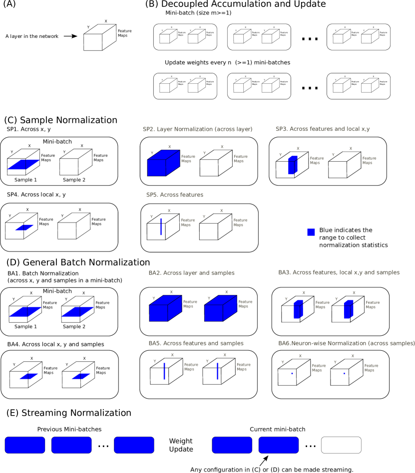
A natural and biologically-inspired extension of these methods would be Streaming Normalization: normalization statistics are collected in an online fashion from all previously seen training samples (and all timesteps if recurrent). We found numerous advantages associated with this approach: 1. it naturally supports pure online learning or learning with small mini-batches. 2. for recurrent learning, it is more biologically-plausible since a unique set of normalization statistics is maintained for all timesteps. 3. it performs well out of the box in all learning scenarios (e.g., online learning, batch learning, fully-connected, convolutional, feedforward, recurrent and mixed — recurrent and convolutional). 4. it offers a new direction of designing normalization algorithms, since the idea of maintaining online estimates of normalization statistics is independent from other design choices, and as a result any existing algorithm (e.g., in Figure 1 C and D) can be extended to a “streaming” setting.
We also propose Lp normalization: instead of normalizing by the second moment like BN, one can normalize by the p-th root of the p-th absolute moment (See Section 3.4 for details). In particular, L1 normalization works as well as the conventional approach (i.e., L2) in almost all learning scenarios. Furthermore, L1 normalization is easier to implement: it is simply the average of absolute values. We believe it can be used to simplify and speed up BN and our Streaming Normalization in GPGPU, dedicated hardware or embedded systems. L1 normalization may also be more biologically-plausible since the gradient of the absolute value is trivial to implement, even for biological neurons.
In the following section, we introduce a simple training scheme, a minor but necessary component of our formulation.
2 Online and Batch Learning with “Decoupled Accumulation and Update”
Although it is not our main result, we discuss a simple but to the best of our knowledge less explored111We are not aware of this approach in the literature. If there is, please inform us. training scheme we call a “Decoupled Accumulation and Update” (DAU).
Conventionally, the weights of a neural network are updated every mini-batch. So the accumulation of gradients and weights update are coupled. We note that a general formulation would be that while for every mini-batch the gradients are still accumulated, one does not necessarily update the weights. Instead, the weights are updated every mini-batches. The gradients are cleared after each weight update. Two parameters characterize this procedure: Samples per Batch (S/B) and Batch per Update (B/U) . In conventional training, .
Note that this procedure is similar to but distinct from simply training larger mini-batches since every mini-batch arrives in a purely online fashion so one cannot look back into any previous mini-batches. For example, if batch normalization is present, performing this procedure with S/B and B/U is different from that with S/B and B/U.
If , it reduces to a pure online setting where one sample arrives at a time. The key advantage of this proposal over conventional training is that we explicitly require less frequent (but more robust) weight updates. The memory requirement (in additional to storing the network weights) is storing samples and related activations.
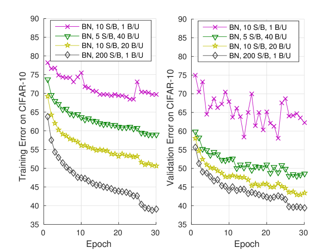
This training scheme generalizes the conventional approach, and we found that merely applying this approach greatly mitigated (although not completely solved) the catastrophic failure of training batch normalization with small mini-batches (See Figure 4). Therefore, we will use this formulation throughout our paper.
We also expect this scheme to benefit learning sequential recurrent networks with varying input sequence lengths. Sometimes it is more efficient to pack in a mini-batch training samples with the same sequence length. If this is the case, our approach predicts that it would be desirable to process multiple such mini-batches with varying sequence lengths before a weight update. Accumulating gradients from training different sequence lengths should provide a more robust update that works for different sequence lengths, thus better approximating the true gradient of the dataset.
In Streaming Normalization with recurrent networks, it is often beneficial to learn with (i.e., more than one batch per update). The first mini-batch collects all the normalization statistics from all timesteps so that later mini-batches are normalized in a more stable way.
3 A General Framework for Normalization
We propose a general framework to describe different normalization algorithms. A normalization can be thought of as a process of modifying the activation of a neuron using some statistics collected from some reference activations. We adopt three terms to characterize this process: A Normalization Operation (NormOP) is a function that is applied to each neuron to modify its value from to , where is the Normalization Statistics (NormStats) for this neuron. NormStats is any data required to perform NormOP, collected using some function , where is a set of activations (could include ) called Normalization Reference (NormRef). Different neurons may or may not share NormRef and NormStats.
This framework captures many previous normalizations algorithms as special cases. For example, the original Batch Normalization (BN) [Ioffe and Szegedy, 2015] can be described as follows: the NormRef for each neuron is all activations in the same channel of the same layer and same batch (See Figure 1 C for illustration). The NormStats are ={,} — the mean and standard deviation of the activations in NormRef. The NormOp is N(,{,}) =
For the recent Layer Normalization [Ba et al., 2016], NormRef is all activations in the same layer (See Figure 1 C). The NormStats and NormOp are the same as BN.
We group normalization algorithms into three categories:
In the following sections, we detail each algorithm and provide pseudocode.
3.1 Sample Normalization
Sample normalization is the simplest category among the three. NormStats are collected only using the activations in the current layer of current sample. The computation is the same at training and test times. It handles online learning naturally. Layer Normalization [Ba et al., 2016] is an example of this category. More examples are shown in Figure 1 C.
3.2 General Batch Normalization
In General Batch Normalization (GBN), NormStats are collected in some way using the activations from all samples in a training mini-batch. Note that one cannot really compute the batch NormStats at test time since test samples should be handled independently from each other, instead in a batch. To overcome this, one can simply compute running estimates of training NormStats and use them for testing (e.g., the original Batch Normalization [Ioffe and Szegedy, 2015] computes moving averages).
3.3 Streaming Normalization
Finally, we present the main results of this paper. We propose Streaming Normalization: NormStats are collected in an online fashion from all past training samples. The main challenge of this approach is that it introduces infinitely long dependencies throughout the neuron’s activation history — every neuron’s current activation depends on all previously seen training samples.
It is intractable to perform exact backpropagation on this dependency graph for the following reasons: there is no point backpropagating beyond the last weight update (if any) since one cannot redo the weight update. This, on the other hand, would imply that one cannot update the weights until having seen all future samples. Even backpropagating within a weight update (i.e., the interval between two weight updates, consisting of mini-batches) turns out to be problematic: one is usually not allowed to backpropagate to the previous several mini-batches since they are discarded in many practical settings.
For the above reasons, we abandoned the idea of performing exact backpropagation for streaming normalization. Instead, we propose two simple heuristics: Streaming NormStats and Streaming Gradients. They are discussed below and the pseudocode is shown in Algorithm 5 and Algorithm 6.
3.3.1 Streaming NormStats
Streaming NormStats is a natural requirement of Streaming Normalization, since NormStats are collected from all previously seen training samples. We maintain a structure/table to keep all the information needed to generate a good estimate of NormStats. and update it using a function everytime we encounter a new training sample. Function also generates the current estimate of NormStats called . We use to normalize instead of . See Algorithm 5 for details.
There could be many potential designs for and , and in our experiments we explored a particular version: we compute two sets of running estimates to keep track of the long-term and short-term NormStats: .
-
•
Short-term NormStats is the exact average of NormStats since the last weight update. The keeps track of the number of times a different is encountered to compute the exact average of .
-
•
Long-term NormStats is an exponential average of since the beginning of training.
Whenever the weights of the network is updated: , is reset to 0 and is set to empty. In our experiments, so that an exponential average of is maintained in .
In our implementation, before testing the model, the last weight update is NOT performed, and is also NOT cleared, since is needed for testing 222It also possible to simply store the last computed in training for testing, instead of storing and re-computing in testing. These two options are mathematically equivalent.
In addition to updating in the way described above, the function also computes . Finally, is used for normalization.
3.3.2 Streaming Gradients
We maintain a structure/table to keep all the information needed to generate a good estimate of gradients of NormStats and update it using a function everytime backpropagation reaches this layer. Function also generates the current estimate of gradients of NormStats called . We use for further backpropagation instead of . See Algorithm 6 for details.
Again, there could be many potential designs for and , and we explored a particular version: we compute two sets of running estimates to keep track of the long-term and short-term gradients of NormStats: .
-
•
Short-term Gradients of NormStats is the exact average of gradients of NormStats since the last weight update. The keeps track of the number of times a different is encountered to compute the exact average of .
-
•
Long-term Gradients of NormStats is an exponential average of since the beginning of training.
Whenever the weights of network is updated: , is reset to 0 and is set to empty. In our experiments, so that an exponential average of is maintained in .
In addition to updating in the way described above, the function also computes . Finally, is used for further backpropagation.
3.3.3 A Summary of Streaming Normalization Design and Hyperparameters
The NormOp used in this paper is N(,{,}) = , the same as what is used by BN. The NormStats are collected using one of the Lp normalization schemes described in Section 3.4.
With our particular choices of , , and , the following hyperparameters uniquely characterize a Streaming Normalization algorithm: , , , samples per batch , batches per update and a choice of mini-batch NormRef (i.e., SP1-SP5, BA1-BA6 in Figure 1 C and D).
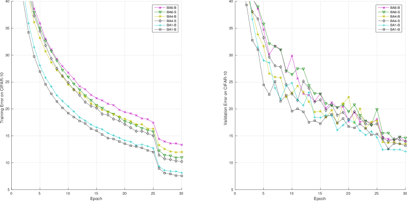
Unless mentioned otherwise, we use BA1 in Figure 1 D as the NormRef throughout the paper. We also demonstrate the use of other NormRefs (BA4 and BA6) in the Appendix Figure A1.
An important special case: If , we ignore all NormStats and gradients beyond the current mini-batch. The algorithm reduces to exactly the GBN algorithm. So Streaming Normalization is strictly a generalization of GBN and thus also captures the original BN [Ioffe and Szegedy, 2015] as a special case. Recall from Section 3.3.1 that is NOT cleared before testing the model. Thus for testing, NormStats are inherited from the last training mini-batch. It works well in practice.
Unless mentioned otherwise, we set , , , , , . We leave it to future research to explore different choices of hyperparameters (and perhaps other and ).
3.3.4 Implementation Notes
One minor drawback of not performing exact backpropagation is that it may break the gradient check of the entire model. One solution coulde be: (1) perform gradient check of the model without SN and then add a correctly implemented SN. (2) make sure the SN layer is correctly coded (e.g., by reducing it to standard BN using the hyperparameters discussed above and then perform gradient check).
3.4 Lp Normalization: Calculating NormStats with Different Orders of Moments
Let us discuss the function for calculating NormStats. There are several choices for this function. We propose Lp normalization. It captures the previous mean-and-standard-deviation normalization as a special case.
First, mean is always calculated the same way — the average of the activations in NormRef. The divisive factor , however, can be calculated in several different ways. In Lp Normalization, is chosen to be the -th root of the -th Absolute Moment.
Here the Absolute Moment of a distribution about a point is:
| (1) |
and the discrete form is:
| (2) |
Lp Normalization can be performed with three settings:
-
•
Setting A: is the -th root of the -th absolute moment of all activations in NormRef with being the mean of NormRef.
-
•
Setting B: is the -th root of the -th absolute moment of all activations in NormRef with being the running estimate of the average.
-
•
Setting C: is the -th root of the -th absolute moment of all activations in NormRef with being 0.
Most of these variants have similar performance but some are better in some situations.
We call it Lp normalization since it is similar to the norm in the space.
Setting B and C are better for online learning since A will give degenerate result (i.e., ) when there is only one sample in NormRef. Empirically, when there are enough samples in a mini-batch, A and B perform similarly.
We discuss several important special cases:
Special Case A-2: setting A with n=2, is the standard deviation (square root of the 2nd moment) of all activations in NormRef. This setting is what is used by Batch Normalization [Ioffe and Szegedy, 2015] and Layer Normalization [Ba et al., 2016].
Special Case p=1: Whenever p=1, is simply the average of absolute values of activations. This setting works virtually the same as p=2, but is much simpler to implement and faster to run. It might also be more biologically-plausible, since the gradient computations are much simpler.
3.5 Separate Learnable Bias and Gain Parameters
The original Batch Normalization [Ioffe and Szegedy, 2015] also learns a bias and a gain (i.e., shift and scaling) parameter for each feature map. Although not usually done, but clearly these shift and scaling operations can be completely separated from the normalization layer. We implemented them as a separate layer following each normalization layer. These parameters are learned in the same way for all normalization schemes evaluated in this paper.
4 Generalization to Recurrent Learning
In this section, we generalize Sample Normalization, General Batch Normalization and Streaming Normalization to recurrent learning. The difference between recurrent learning and feedforward learning is that for each training sample, every hidden layer of the network receives activations , instead of only one.
4.1 Recurrent Sample Normalization
Sample Normalization naturally generalizes to recurrent learning since all NormStats are collected from the current layer of the current timestep. Training and testing algorithms remain the same.
4.2 Recurrent General Batch Normalization (RGBN)
The generalization of GBN to recurrent learning is the same as what was proposed by [Liao and Poggio, 2016] and [Cooijmans et al., 2016]. The training procedure is exactly the same as before (Algorithm 3 and Algorithm 4). For testing, one set of running estimates of NormStats is maintained for each timestep.
4.3 Recurrent Streaming Normalization
Extending Streaming Normalization to recurrent learning is straightforward – we not only stream through all the past samples, but also through all past timesteps. Thus, we maintain a unique set of running estimates of NormStats for all timesteps. This is more biologically-plausible and memory efficient than the above approach (RGBN).
Again, another way of viewing this algorithm is that the same Streaming Normalization layers described in Algorithm 5 and 6 are used in the original (instead of the unrolled) recurrent network. All unrolled versions of the same layer share running estimates of NormStats and other related data.
One caveat is that as time proceeds, the running estimates of NormStats are slightly modified. Thus when backpropagation reaches the same layer again, the NormStats are slightly different from the ones originally used for normalization. Empirically, it seems to not cause any problem on the performance. Training with “decoupled accumulation update” with Batches per Update (B/U) > 1 333B/U=2 is often enough can also mitigate this problem, since it makes NormStats more stable over time.
5 Streaming Normalized RNN and GRU
In our character-level language modeling task, we tried Normalized Recurrent Neural Network (RNN) and Normalized Gated Recurrent Unit (GRU) [Chung et al., 2014]. Let us use Norm(.) to denote a normalization, which can be either Sample Normalization, General Batch Normalization or Streaming Normalization. A bias and gain parameter is also learned for each neuron. We use NonLinear to denote a nonlinear function. We used hyperbolic tangent (tanh) nonlinearity in our experiments. But we observed ReLU also works. is the hidden activation at time . is the network input at time . denotes the weights. denotes elementwise multiplication.
Normalized RNN
| (3) |
Normalized GRU
| (4) | |||
| (5) | |||
| (6) | |||
| (7) |
6 Related Work
[Laurent et al., 2015] and [Amodei et al., 2015] used Batch Normalization (BN) in stacked recurrent networks, where BN was only applied to the feedforward part (i.e., “vertical” connections, input to each RNN), but not the recurrent part (i.e., “horizontal”, hidden-to-hidden connections between timesteps). [Liao and Poggio, 2016] and [Cooijmans et al., 2016] independently proposed applying BN in recurrent/hidden-to-hidden connections of recurrent networks, but separate normalization statistics must be maintained for each timestep. [Liao and Poggio, 2016] demonstrated this idea with deep multi-stage fully recurrent (and convolutional) neural networks with ReLU nonlinearities and residual connections. [Cooijmans et al., 2016] demonstrated this idea with LSTMs on language processing tasks and sequential MNIST. [Ba et al., 2016] proposed Layer Normalization (LN) as a simple normalization technique for online and recurrent learning. But they observed that LN does not work well with convolutional networks. [Salimans and Kingma, 2016] and [Neyshabur et al., 2015] studied normalization using weight reparameterizations. An early work by [Ullman and Schechtman, 1982] mathematically analyzed a form of online normalization for visual perception and adaptation.
7 Experiments
7.1 CIFAR-10 architectures and Settings
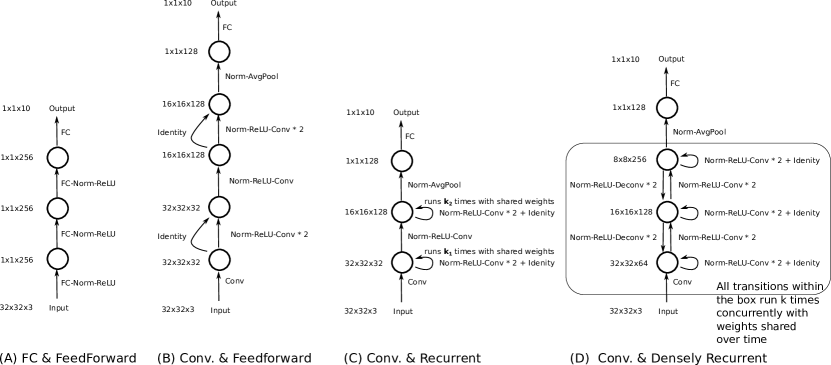
We evaluated the normalization techniques on CIFAR-10 dataset using feedforward fully-connected networks, feedforward convolutional network and a class of convolutional recurrent networks proposed by [Liao and Poggio, 2016]. The architectural details are shown in Figure 2. We train all models with learning rate 0.1 for 25 epochs and 0.01 for 5 epochs. Momentum 0.9 is used. We used MatConvNet [Vedaldi and Lenc, 2015] to implement our models.
7.2 Lp Normalization
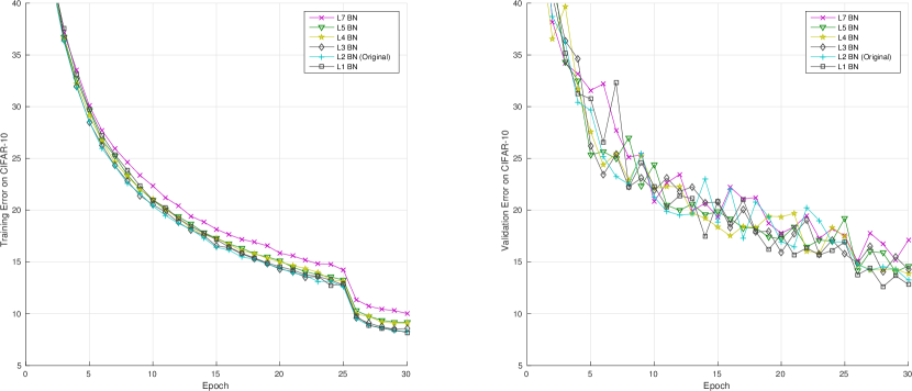
We show BN with Lp normalization in Figure 3. Note that Lp normalization can be applied to Layer Normalization and all other normalizations show in 1 C and D. L1 normalization works as well as L2 while being simpler to implement and faster to compute.
7.3 Online Learning or Learning with Very Small Mini-batches
We perform online learning or learning with small mini-batches using architecture A in Figure 2.
Plain Mini-batch vs. Decoupled Accumulation and Update (DAU): We show in Figure 4 comparisons between conventional mini-batch training and Decoupled Accumulation and Update (DAU).
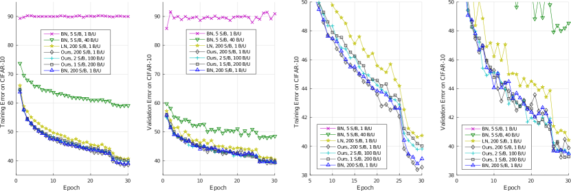
Layer Normalization vs. Batch Normalization vs. Streaming Normalization: We compare in Figure 5 Layer Normalization, Batch Normalization and Streaming Normalization with different choices of S/B and B/U.
7.4 Evaluating Variants of Batch Normalization
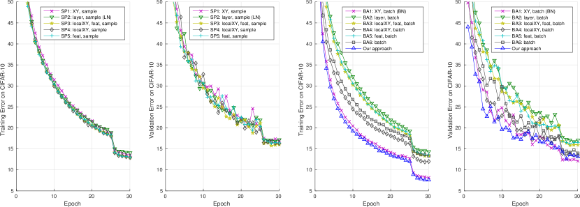
Feedforward Convolutional Networks: In Figure 6, we tested algorithms shown in Figure 1 C and D using the architecture B in Figure 2. We also show the performance of our Streaming Normalization for reference.
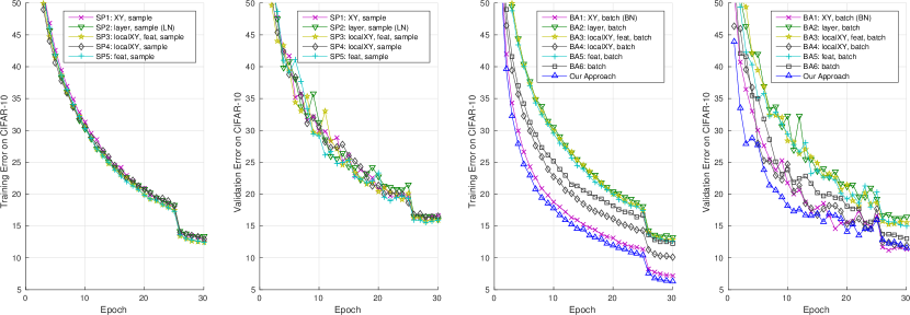
ResNet-like convolutional RNN: In Figure 7, we tested algorithms shown in Figure 1 C and D using the architecture C in Figure 2. We also show the performance of our Streaming Normalization for reference.
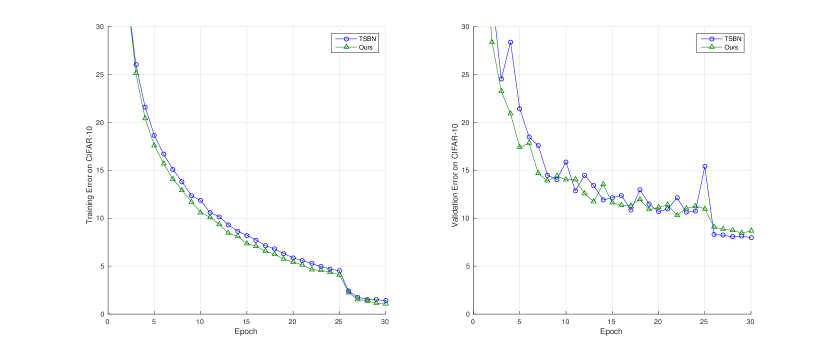
Densely Recurrent Convolutional Network: In Figure 8, we tested Time-Specific Batch Normalization and Streaming Normalization on the architecture D in Figure 2.
7.5 More Experiments on Streaming Normalization
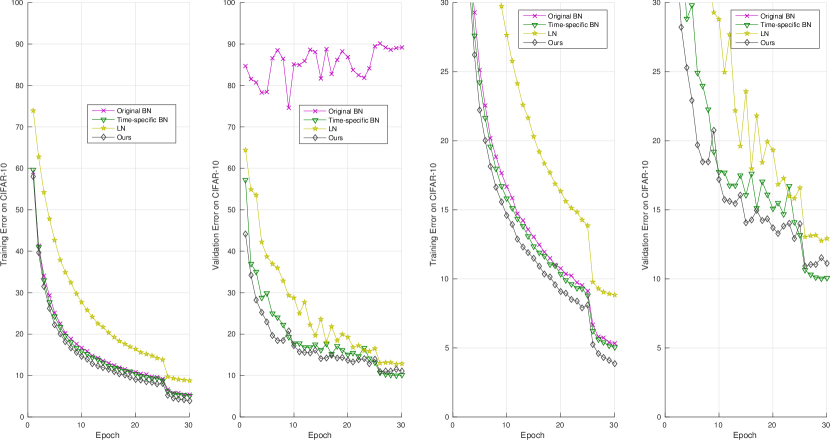
In Figure 9, we compare the performances of original BN (i.e., NormStats shared over time), time-specific BN, layer normalization and streaming normalization on a recurrent and convolutional network shown in Figure 2 C.
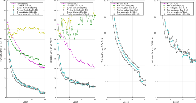
We evaluated different choices of hyperparameter , and in Figure 10.
7.6 Recurrent Neural Networks for Character-level Language Modeling
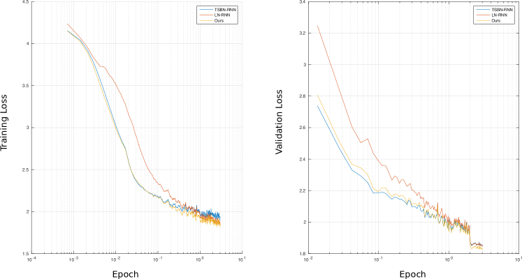
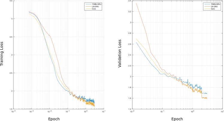
We tried our simple implementations of vanilla RNN and GRU described in Section 5. The RNN and GRU both have 1 hidden layer with 100 units. Weights are updated using the simple Manhattan update rule described in [Liao et al., 2015]. The models were trained with learning rate 0.01 for 2 epochs and 0.001 for 1 epoch on a text file of all Shakespeare’s work concatenated. We use 99% the text file for training and 1% for validation. The training and validation softmax losses are reported. Training losses are from mini-batches so they are noisy, and we smoothed them using moving averages of 50 neighbors (using the Matlab smooth function). The test loss on the entire validation set is evaluated and recorded every 20 mini-batches. We show in Figure 11 and 12 the performances of Time-specific Batch Normalization, Layer Normalization and Streaming Normalization. Truncated BPTT was performed with 100 timesteps.
8 Discussion
Biological Plausibility
We found that the simple “Neuron-wise normalization” (BA6 in Figure 1 D) performs very well (Figure 6 and 7). This setting does not require collecting normalization statistics from any other neurons. We show the streaming version of neuron-wise normalization in Figure A1, and the performance is again competitive. In neuron-wise normalization, each neuron simply maintains running estimates of its own mean and variance (and related gradients), and all the information is maintained locally. This approach may serve as a baseline model for biological homeostatic plasticity mechanisms (e.g., Synaptic Scaling) [Turrigiano and Nelson, 2004, Stellwagen and Malenka, 2006, Turrigiano, 2008], where each neuron internally maintains some normalization/scaling factors that depend on neuron’s firing history and can be applied and updated in a pure online fashion.
Lp Normalization
Our observations about Lp normalization have several biological implications: First, we show that most Lp normalizations work similarly, which suggests that there might exist a large class of statistics that can be used for normalization. Biological systems could implement any of these methods to get the same level of performance. Second, L1 normalization is particularly interesting, since its gradient computations are much easier for biological neurons to implement.
As an orthogonal direction of research, it would also be interesting to study the relations between our Lp normalization (standardizing the average Lp norm of activations) and Lp regularization (discounting the the Lp norm of weights, e.g., L1 weight decay).
Theoretical Understanding
Although normalization methods have been empirically shown to significantly improve the performance of deep learning models, there is not enough theoretical understanding about them. Activation-normalized neurons behave more similarly to biological neurons whose activations are constrained into a certain range: is it a blessing or a curse? Does it affect approximation bounds of shallow and deep networks [Mhaskar et al., 2016, Mhaskar and Poggio, 2016]? It would also be interesting to see if certain normalization methods can mitigate the problems of poor local minima and saddle points, as the problems have been analysed without normalization [Kawaguchi, 2016].
Internal Covariant Shift in Recurrent Networks
Note that our approach (and perhaps the brain’s “synaptic scaling”) does not normalize differently for each timestep. Thus, it does not naturally handle internal covariant shift [Ioffe and Szegedy, 2015] (more precisely, covariate shift over time) in recurrent networks, which was the main motivation of the original Batch Normalization and Layer Normalization. Our results seem to suggest that internal covariate shift is not as hazardous as previously believed as long as the entire network’s activations are normalized to a good range. But more research is needed to answer this question.
Acknowledgments
This work was supported by the Center for Brains, Minds and Machines (CBMM), funded by NSF STC award CCF – 1231216.
References
- [Amodei et al., 2015] Amodei, D., Anubhai, R., Battenberg, E., Case, C., Casper, J., Catanzaro, B., Chen, J., Chrzanowski, M., Coates, A., Diamos, G., et al. (2015). Deep speech 2: End-to-end speech recognition in english and mandarin. arXiv preprint arXiv:1512.02595.
- [Ba et al., 2016] Ba, J. L., Kiros, J. R., and Hinton, G. E. (2016). Layer normalization. arXiv preprint arXiv:1607.06450.
- [Chung et al., 2014] Chung, J., Gulcehre, C., Cho, K., and Bengio, Y. (2014). Empirical evaluation of gated recurrent neural networks on sequence modeling. arXiv preprint arXiv:1412.3555.
- [Cooijmans et al., 2016] Cooijmans, T., Ballas, N., Laurent, C., and Courville, A. (2016). Recurrent batch normalization. arXiv preprint arXiv:1603.09025.
- [He et al., 2015] He, K., Zhang, X., Ren, S., and Sun, J. (2015). Deep residual learning for image recognition. arXiv preprint arXiv:1512.03385.
- [Ioffe and Szegedy, 2015] Ioffe, S. and Szegedy, C. (2015). Batch normalization: Accelerating deep network training by reducing internal covariate shift. arXiv preprint arXiv:1502.03167.
- [Kawaguchi, 2016] Kawaguchi, K. (2016). Deep learning without poor local minima. In Advances in Neural Information Processing Systems (NIPS). to appear.
- [Laurent et al., 2015] Laurent, C., Pereyra, G., Brakel, P., Zhang, Y., and Bengio, Y. (2015). Batch normalized recurrent neural networks. arXiv preprint arXiv:1510.01378.
- [Liao et al., 2015] Liao, Q., Leibo, J. Z., and Poggio, T. (2015). How important is weight symmetry in backpropagation? arXiv preprint arXiv:1510.05067.
- [Liao and Poggio, 2016] Liao, Q. and Poggio, T. (2016). Bridging the gaps between residual learning, recurrent neural networks and visual cortex. arXiv preprint arXiv:1604.03640.
- [Mhaskar et al., 2016] Mhaskar, H., Liao, Q., and Poggio, T. (2016). Learning real and boolean functions: When is deep better than shallow. arXiv preprint arXiv:1603.00988.
- [Mhaskar and Poggio, 2016] Mhaskar, H. and Poggio, T. (2016). Deep vs. shallow networks: An approximation theory perspective. arXiv preprint arXiv:1608.03287.
- [Neyshabur et al., 2015] Neyshabur, B., Salakhutdinov, R. R., and Srebro, N. (2015). Path-sgd: Path-normalized optimization in deep neural networks. In Advances in Neural Information Processing Systems, pages 2422–2430.
- [Salimans and Kingma, 2016] Salimans, T. and Kingma, D. P. (2016). Weight normalization: A simple reparameterization to accelerate training of deep neural networks. arXiv preprint arXiv:1602.07868.
- [Stellwagen and Malenka, 2006] Stellwagen, D. and Malenka, R. C. (2006). Synaptic scaling mediated by glial tnf-. Nature, 440(7087):1054–1059.
- [Turrigiano and Nelson, 2004] Turrigiano, G. and Nelson, S. (2004). Homeostatic plasticity in the developing nervous system. Nature Reviews Neuroscience, 5(2):97–107.
- [Turrigiano, 2008] Turrigiano, G. G. (2008). The self-tuning neuron: synaptic scaling of excitatory synapses. Cell, 135(3):422–435.
- [Ullman and Schechtman, 1982] Ullman, S. and Schechtman, G. (1982). Adaptation and gain normalization. Proceedings of the Royal Society of London B: Biological Sciences, 216(1204):299–313.
- [Vedaldi and Lenc, 2015] Vedaldi, A. and Lenc, K. (2015). Matconvnet: Convolutional neural networks for matlab. In Proceedings of the 23rd Annual ACM Conference on Multimedia Conference, pages 689–692. ACM.
Appendix A Other Variants of Streaming Normalization
