A Heterogeneous Out-of-Equilibrium Nonlinear $q$-Voter Model with Zealotry

Abstract

We study the dynamics of the out-of-equilibrium nonlinear $q$-voter model with two types of susceptible voters and zealots, introduced in [EPL 113, 48001 (2016)]. In this model, each individual supports one of two parties and is either a susceptible voter of type $q_{1}$ or $q_{2}$, or is an inflexible zealot. At each time step, a $q_{i}$-susceptible voter ($i=1,2$) consults a group of $q_{i}$ neighbors and adopts their opinion if all group members agree, while zealots are inflexible and never change their opinion. This model violates detailed balance whenever $q_{1}\neq q_{2}$ and is characterized by two distinct regimes of low and high density of zealotry. Here, by combining analytical and numerical methods, we investigate the non-equilibrium stationary state of the system in terms of its probability distribution, non-vanishing currents and unequal-time two-point correlation functions. We also study the switching time properties of the model by exploiting an approximate mapping onto the model of [Phys. Rev. E 92, 012803 (2015)] that satisfies the detailed balance, and we outline some properties of the model near criticality.

I Introduction

Parsimonious individual-based models have been commonly used to describe collective social phenomena for more than four decades Schelling (1969); *schelling1971dynamic; *schelling1978micromotives. In particular, statistical physics models have proven especially well-suited to reveal the micro-macro connections in social dynamics and to help reveal the relationships existing between phenomena appearing across disciplines (like biology, ecology, economics) Castellano et al. (2009a). In particular, the voter model (VM) Liggett (1985) serves as a reference to describe the evolution of opinions in interacting populations Castellano et al. (2009a); Galam (2012); *sen2013sociophysics. It is however well established that the VM is built on a number of oversimplified assumptions: For instance, the VM considers that all voters are similar: In the absence of any self-confidence, they change their their opinion by imitating neighbors. This mechanism of conformity by imitation does not allow us to maintain social diversity in the long run, but always leads to a consensus. However, social scientists have shown that the collective dynamics of a society greatly depends on the different responses to stimuli by the members of a society Granovetter (1978); Latané (1981); *nail2000proposal; Asch (1955); *milgram1969note. A simple way to accommodate a population with different levels of confidence is to assume that some agents are “zealots” and either favor one opinion Mobilia (2003); *mobilia2005voting or inflexibly maintain a fixed opinion Mobilia et al. (2007). Since the introduction of zealots in the VM, the effect of zealotry has been studied in other models of social dynamics Galam and Jacobs (2007); *sznajdweron2011phase; *acemoglu2013opinion; *nyczka2013anticonformity; *yildiz2013binary; *palombi2014stochastic; *verma2014impact; *waagen2015effect; *arendt2015opinions and in various contexts Masuda (2015); *xie2011social; *masuda2012evolution; *borile2015coexistence; *mobilia2012stochastic; *mobilia2013evolutionary; *mobilia2013reply; *mobilia2013commitment; *szolnoki2016zealots.

In this work, we focus on the so-called two-state nonlinear $q$-voter model ($q$VM) Castellano et al. (2009b). In this variant of the VM, that has received much attention recently Slanina et al. (2008); *galam2011pitfalls; *przybyla2011exit; *timpanaro2014exit; *timpanaro2015analytical; *jedrzejewski2015oscillating; *javarone2015conformism, each voter can be influenced by a group of $q$ neighbors [Theversionwith$q=2$iscloselyrelatedtothewell-knownmodelsof][]sznajdweron2000opinion; *slanina2003analytical; *lambiotte2008dynamics  . This mimics the fact that group pressure is known to influence the degree of conformity, especially above a group size threshold Asch (1955); *milgram1969note. Furthermore, social scientists have shown that conformity via imitation is a driving mechanism for collective actions that is influenced by the size of social groups, and they also found that conformity can be seriously deflected by individuals (like zealots) that are able to resist group pressure Asch (1955); *milgram1969note; Latané (1981); *nail2000proposal. Motivated by these considerations Latané (1981); *nail2000proposal; Granovetter (1978), the basic features of the $q$VM and zealotry have recently been combined in the $q$-voter model with inflexible zealots ($q$VMZ) Mobilia (2015) and in a heterogeneous counterpart model, called the 2$q$VZ, in which two subgroups of susceptible voters interacting with their neighbors with different $q$’s: namely, with $q_{1}<q_{2}$ Mellor et al. (2016a).

In the $q$VMZ and 2$q$VZ, group-size limited conformity and zealotry are accounted for, and zealots significantly tame the level of social conformity in the population Mobilia (2015); Mellor et al. (2016a). Furthermore, the dynamics of the $q$VMZ and 2$q$VZ in a well-mixed population is similar and is characterized by two phases as in systems in thermal equilibrium: Below a critical level of zealotry, the opinion distribution transitions from single-peaked becomes bimodal and, in finite populations, the dynamics is characterized by the fluctuation-driven switching between two states Mobilia (2015); Mellor et al. (2016a). Yet, while the $q$VMZ of Ref. Mobilia (2015) obeys detailed balance and its stationary distribution can be obtained exactly, this is not the case of the 2$q$VZ even in the simple case of a well-mixed population when the system relaxes into a non-equilibrium steady state (NESS) Mellor et al. (2016a). The fact that the 2$q$VZ does not obey detailed balance has many important statistical physics consequences: There is generally no simple way to obtain the NESS distribution Hill (1966), while persistent probability currents are responsible for subtle oscillations and non-trivial correlation functions Zia and Schmittmann (2007); Mellor et al. (2016a). From a social dynamics viewpoint, the composition of the society being very heterogeneous, it would be relevant to consider models with a distribution of $q$’s that would reflect different responses to multiple social stimuli Granovetter (1978). While analytical progress appears to be difficult in such a general case, much can be learnt about the influence of being out-of-equilibrium on the social dynamics by considering the simple 2$q$VZ whose detailed analysis is presented here. In particular, we are able to show that susceptible voters with smaller $q$ change their opinion more quickly and drive those in the other subgroup, and directed, yet subtle, oscillations associated with fluctuating quantities can be measured [][(SeealsoarXiv:1610.02976)]zia2016manifest.

In this work, we therefore focus on the 2$q$VZ and characterize the properties of its NESS in terms of the master equation, stochastic simulations and continuum approximations based on mean-field and Fokker-Planck equations. While a brief account of some of these features was given in Ref. Mellor et al. (2016a), here we considerably generalize that study and also investigate the switching dynamics of the 2$q$VZ.

The remainder of this paper is organized as follows: The details of the 2$q$VZ are specified in the next section, along with the underlying master equation. The microscopic characterization of the NESS in terms of the master equation and relevant observables is addressed in Sec. III. Section IV is dedicated to the continuum approximation of the $2q$VZ dynamics in terms of mean-field rate equations and through a linear Gaussian approximation (LGA) of the underlying Fokker-Planck equation (for a system of large but finite size)  Lax (1966); Weiss (2003); *weiss2007fluctuation; Zia and Schmittmann (2007). This allows us to show in some details, how the LGA offers the best insight into probability currents and their manifestations in the $2q$VZ’s NESS far from criticality, as explained in Sec. IV.B. In Sec. IV.C, we exploit a Fokker-Planck formulation to shed light on the switching time properties of the 2$q$VZ via an approximate mapping onto the $q$VMZ whereas the behavior near criticality is briefly discussed in Sec. IV.D. While most examples given in Sec. IV are concerned with the case of symmetric zealotry (the same number of zealots for each party), the generalization to asymmetric zealotry is addressed in Sec. V. We also give a number of analytical and computational details in a series of appendixes. We end with a summary, as well as an outlook for future research. It is worth noting that while our general analysis applies to any values of $q_{1}$ and $q_{2}$, for the sake of simplicity and without loss of generality, the numerical examples reported in our figures have been obtained for $q_{1,2}=1,2$.

II The 2$q$ Voter Model with Zealotry (2$q$VZ)

Figure 1: (Color online). Illustration of the 2$q$VZ dynamics: (a) the system consists of zealots, $q_{1}$-, and $q_{2}$- susceptibles; each can hold one of two opinions (green/black or blue/grey). (b) A $q_{i}$ susceptible picks $q_{i}$ neighbors at random. Here, $q_{2}=2$. (c) If the picked neighbors have same opinion, the focal susceptible voter adopts their opinion, otherwise no change occurs.

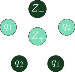
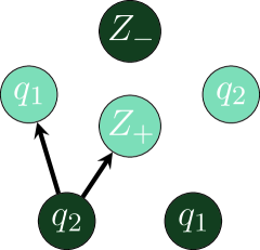
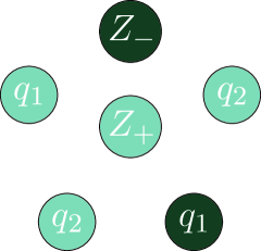
The 2$q$VZ consists of a population of $N$ voters who hold one of two opinions, denoted by $\pm 1$. A fraction of the population are inflexible zealots that never change their opinion Mobilia et al. (2007); Mobilia (2015), the number of which are denoted by $Z_{\pm}$. The remaining population consists of $S=S_{1}+S_{2}$ swing voters of two types, $q_{1}$ and $q_{2}$ (known as $q_{i}$-susceptibles, $i=1,2$): $S_{1}$ of the swing voters are of type $q_{1}$ and there are $S_{2}$ swing voters of type $q_{2}$. In our model, the behavior of each voter is fixed, so that $Z_{\pm}$ and $S_{i}$ are conserved, with $S_{1}+S_{2}+Z_{+}+Z_{-}=N$. As illustrated in Fig. 1, the evolution of the 2$q$VZ is such that at each update attempt (a) a (focal) voter is chosen at random. (b) If the chosen voter is a zealot then no further action is taken. If the focal voter is a $q_{i}$-susceptible however, then the opinions of a random group of $q_{i}$ of its neighbors (repetition is allowed) are collected. (c) If the $q_{i}$ neighbors have the same opinion that differs from that of the focal voter, the latter adopts the opinion of the group. If there is no consensus within the $q_{i}$-group, the opinion of the focal voter does not change. Here, for the sake of simplicity we consider a well-mixed population, i.e., each voter can be thought of as one of the $N$ nodes of a complete graph and all other voters are “neighbors”.

II.1 Microscopic Description with a Master Equation

In the absence of explicit spatial structure, the configuration space is a discrete set of $S_{1}\times S_{2}$ points and the system state is completely specified by the pair $\vec{n}:=(n_{1},n_{2})$ where $n_{i}$ is the number of susceptible voters of type $i$ holding the opinion $+1$. In each update attempt, the system may, or may not, step to one of its four nearest neighboring points. In other words the allowed changes are in the set $\left\{\pm\vec{e}_{1},\pm\vec{e}_{2}\right\}$, with $\vec{e}_{1}:=(1,0)$ and $\vec{e}_{2}:=(0,1)$. Thus, we may regard the evolution of the 2$q$VZ as a two-dimensional random walker with inhomogeneous and biased rates. Such a stochastic process can be readily described by a master equation (ME) for the evolution of $P(\vec{n},T)$, the probability of finding the system in state $\vec{n}$ after $T$ discrete time steps (or update attempts) from starting in an initial configuration $\vec{n}_{0}$. One of our main interests is in the unique stationary distribution, which has no dependence on the initial configuration $\vec{n}_{0}$, and we can therefore omit any reference to $\vec{n}_{0}$.

For any discrete Markov process, the ME can be written as

$$P(\vec{n}^{\prime},T+1)=\sum_{\vec{n}}\mathcal{G}(\vec{n}^{\prime},\vec{n})P(\vec{n},T)$$ (1)

where $\mathcal{G}$ is known as the transition matrix, or evolution operator. In our case, since $\vec{n}^{\prime}\in\{\vec{n},\vec{n}\pm\vec{e}_{1},\vec{n}\pm\vec{e}_{2}\}$, so that, an explicit form for $\mathcal{G}$ is

$$\mathcal{G}(\vec{n}^{\prime},\vec{n}) = \delta\left(n_{1}^{\prime},n_{1}\right)\delta\left(n_{2}^{\prime},n_{2}\right)W^{0}(\vec{n})$$

$$+ \sum_{i=1,2,j\neq i}\delta\left(n_{i}^{\prime},n_{i}+1\right)\delta\left(n_{j}^{\prime},n_{j}\right)W_{i}^{+}(\vec{n})$$

$$+ \sum_{i=1,2,j\neq i}\delta\left(n_{i}^{\prime},n_{i}-1\right)\delta\left(n_{j}^{\prime},n_{j}\right)W_{i}^{-}(\vec{n}).$$

Here, $W^{0}(\vec{n})$ represents the probability for the system to remain unchanged, while $W_{1}^{\pm}(\vec{n})$ and $W_{2}^{\pm}(\vec{n})$ stand for the stepping probabilities associated with $\vec{n}\rightarrow\vec{n}\pm\vec{e}_{1}$ and $\vec{n}\rightarrow\vec{n}\pm\vec{e}_{2}$ , respectively. Explicitly , these are

$$W_{i}^{+}(\vec{n}) = \frac{S_{i}-n_{i}}{N}\left(\frac{M}{N-1}\right)^{q_{i}}$$

$$W_{i}^{-}(\vec{n}) = \frac{n_{i}}{N}\left(\frac{N-M}{N-1}\right)^{q_{i}}$$ (3)

$$W^{0}(\vec{n}) = 1-W_{1}^{+}(\vec{n})-W_{1}^{-}(\vec{n})-W_{2}^{+}(\vec{n})-W_{2}^{-}(\vec{n}),$$

where $M=Z_{+}+n_{1}+n_{2}$ is the total number of $+1$ voters before the update. (See (36) in Appendix A for further details.)

Subsequently, we will be interested in the joint probability,

$$\mathcal{P}(\vec{n}^{\prime},T^{\prime};\vec{n},T)=\mathcal{G}^{T^{\prime}-T}(\vec{n}^{\prime},\vec{n})P(\vec{n},T),$$ (4)

for finding the system being in a state $\vec{n}^{\prime}$ at (a later, assuming $T^{\prime}>T$) time $T^{\prime}$ and being in state $\vec{n}$ at time $T$ (see (39)). With these probability distributions, we can compute physical observables such as the average number of $q_{i}$ voters holding opinion $+1$ at time $T$ and two-point correlation functions at general times:

$$\langle n_{i}\rangle_{T} = \sum_{\vec{n}}n_{i}P(\vec{n},T)$$

$$\langle n_{i}^{\prime}n_{j}\rangle_{T^{\prime},T} = \sum_{\vec{n},\vec{n}^{\prime}}n_{i}^{\prime}n_{j}\mathcal{P}(\vec{n}^{\prime},T^{\prime};\vec{n},T).$$

One quantity of particular interest for the study of the 2$q$VZ is the net probability current, given by $\vec{K}(\vec{n};T)=(K_{1},K_{2})$, see (37) in Appendix A. Here, $K_{i}(\vec{n};T)=W_{i}^{+}(\vec{n})P(\vec{n};T)-W_{i}^{-}(\vec{n}^{\prime})P(\vec{n}^{\prime};T)$ denotes the net flow (of probability) from $\vec{n}$ to $\vec{n}^{\prime}\equiv\vec{n}+\vec{e_{i}}$, with $i=1,2$, $\vec{e}_{1}=(1,0)$ and $\vec{e}_{2}=(0,1)$.

II.2 Violation of Detailed Balance

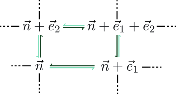
In Ref. Mellor et al. (2016a), we emphasized a distinctive feature of the 2$q$VZ, namely, that its dynamics is a genuine out-of-equilibrium type, contrary to the $q$VMZ Mobilia (2015) model. Hence, detailed balance and time reversal symmetry are violated in the 2$q$VZ. To establish this fact, we apply the Kolmogorov criterion (40) Kolmogorov (1936) on a closed loop consisting of the four $\vec{n}$’s around a square: $\vec{n}\rightarrow\vec{n}+\vec{e}_{1}\rightarrow\vec{n}+\vec{e}_{1}+\vec{e}_{2}\rightarrow\vec{n}+\vec{e}_{2}\rightarrow\vec{n}$, illustrated in Fig. 2. The product of transition probabilities around this loop is

$$W_{1}^{+}\left(\vec{n}\right)W_{2}^{+}\left(\vec{n}+\vec{e}_{1}\right)W_{1}^{-}\left(\vec{n}+\vec{e}_{1}+\vec{e}_{2}\right)W_{2}^{-}\left(\vec{n}+\vec{e}_{2}\right).$$

Meanwhile, the product for the reverse loop is

$$W_{2}^{+}\left(\vec{n}\right)W_{1}^{+}\left(\vec{n}+\vec{e}_{2}\right)W_{2}^{-}\left(\vec{n}+\vec{e}_{1}+\vec{e}_{2}\right)W_{1}^{-}\left(\vec{n}+\vec{e}_{1}\right)$$

so that the ratio of the two probabilities is

$$\left(\frac{M+1}{M}\frac{N-M-1}{N-M-2}\right)^{q_{1}-q_{2}}.$$

Since the quantity in the bracket is strictly greater than unity, this ratio is not unity as long as $q_{1}\neq q_{2}$. Thus, the dynamics of our 2$q$VZ violates the detailed balance. Of course, setting $q_{1}=q_{2}$ we recover the $q$VMZ, for which the above ratio is always unity, confirming that the single-$q$ case of Ref. Mobilia (2015) satisfies the detailed balance.

Figure 2: (Color online). The state space of the 2$q$VZ is of size $(S_{1}+1)\times(S_{2}+1)$ and can be represented as a two-dimensional lattice. The probability of traversing the shown loop clockwise (green/black) does not equal the probability of traversal in the opposite direction (blue/grey). By Kolmogorov’s criterion, the detailed balance is violated; see text.

Violation of detailed balance has a number of consequences on the behavior of a system. These will be scrutinized in the next sections. In particular, we will be mostly interested in the behavior of the stationary state (reached after very long times from any initial $\vec{n}_{0}$), described by the $T$-independent distribution $P^{\ast}\left(\vec{n}\right)$ . From Eq. (1), we see that it is the (right) eigenvector of $\mathcal{G}$ with unit eigenvalue. Meanwhile, the joint distribution in this state will be homogeneous in time and so, depends only on the difference $\tau\equiv T^{\prime}-T:$

$$\mathcal{P}^{\ast}(\vec{n}^{\prime},T^{\prime};\vec{n},T)=\mathcal{G}^{\tau}(\vec{n}^{\prime},\vec{n})P^{\ast}(\vec{n})$$

III Microscopic Characterization of the NESS

As summarized in Appendix A, a significant consequence of detailed balance violation is that the system relaxes into a non-equilibrium steady state (NESS). Typically, finding the associated stationary distribution $P^{\ast}$ is a challenging task . Further, due to the absence of time reversal, this NESS is characterized by non-vanishing probability currents Zia and Schmittmann (2007). Though net currents may flow between any two configurations in general, here they exist only between nearest neighbors, e.g., from $\vec{n}$ to $\vec{n}+\vec{e}_{i}$. Thus, we can denote it by a vector field $\vec{K}^{\ast}$, the components being

$$K_{1}^{\ast}(\vec{n}) = W_{1}^{+}(\vec{n})P^{\ast}(\vec{n})-W_{1}^{-}(\vec{n}+\vec{e}_{1})P^{\ast}(\vec{n}+\vec{e}_{1}),$$ (5)

$$K_{2}^{\ast}(\vec{n}) = W_{2}^{+}(\vec{n})P^{\ast}(\vec{n})-W_{2}^{-}(\vec{n}+\vec{e}_{2})P^{\ast}(\vec{n}+\vec{e}_{2}),$$

Note that $-K_{i}^{\ast}(\vec{n}-\vec{e}_{i})$ is also the net current from $\vec{n}$ to $\vec{n}-\vec{e}_{i}$. In a NESS, the current is divergence-free (see Appendix A). On a lattice, this condition reads

$$0=K_{1}^{\ast}(\vec{n})-K_{1}^{\ast}(\vec{n}-\vec{e}_{1})+K_{2}^{\ast}(\vec{n})-K_{2}^{\ast}(\vec{n}-\vec{e}_{2}).$$ (6)

As a result, the curl of $\vec{K}^{\ast}$ is non-trivial, i.e., $\vec{K}^{\ast}$ forms closed loops, a useful characterization of which is the vorticity, $\omega^{\ast}$ (see Appendix A). On the discrete $S_{1}\times S_{2}$ lattice, any closed loop can be regarded as the sum of elementary loops, each around a square (plaquette). Thus, we associate $\omega^{\ast}$ with a plaquette instead of a site. While the center of a plaquette is located at half integers $(n_{1}+1/2,n_{2}+1/2)$ Mellor et al. (2016b), we will still use $\vec{n}$ for convenience. Thus we write

$$\omega^{\ast}\left(\vec{n}\right)=K_{1}^{\ast}(\vec{n})+K_{2}^{\ast}(\vec{n}+\vec{e}_{1})-K_{1}^{\ast}(\vec{n}+\vec{e}_{2})-K_{2}^{\ast}(\vec{n}).$$ (7)

Of course, $\omega^{\ast}$ is related to the (generalized) discrete Laplacian of $P^{\ast}$ and so, carries information about the curvature of $P^{\ast}$. At the intuitive level, such loops also suggest that one species “following”, or “chasing”, the other (see Fig. 3(b,c)), much like the time-irreversible dynamics of predator-prey systems.

Apart from the vorticity, it is useful to characterize a divergence free vector field as the curl of another. Since our space is two dimensional, this field is a scalar, $\psi^{\ast}$, known in fluid dynamics as the stream function. Thus,

$$K_{i}^{\ast}(\vec{n})=\varepsilon_{ij}\left[\psi^{\ast}\left(\vec{n}\right)-\psi^{\ast}\left(\vec{n}-\vec{e}_{j}\right)\right]$$ (8)

where $\varepsilon_{ij}$ is the two-dimensional Levi-Civita symbol and repeated indices are summed. On our lattice, $\psi^{\ast}$ is also associated with a plaquette so that we can use the same scheme as in $\omega^{\ast}$. If we chose the arbitrary constant in $\psi^{\ast}$ to be zero just outside the $S_{1}\times S_{2}$ rectangle, then we find

$$\psi^{\ast}\left(\vec{n}\right)=\sum_{\ell=0}^{n_{2}}K_{1}^{\ast}(n_{1},\ell)=-\sum_{\ell=0}^{n_{1}}K_{2}^{\ast}(\ell,n_{2}),$$ (9)

For the more familiar continuum versions of $\vec{K}^{\ast}$, $\omega^{\ast}$, and $\psi^{\ast}$; see Appendix A.1.

Finally, in formal analogy with fluid dynamics, we can associate these probability current loops with the concept of probability angular momentum. As $\vec{L}=\int_{\vec{r}}\vec{r}\times\vec{J}\left(\vec{r}\right)$ represents the total angular momentum of a fluid with current density $\vec{J}$, the sum $\sum_{\vec{n}}\left[n_{1}K_{2}^{\ast}(\vec{n})-n_{2}K_{1}^{\ast}(\vec{n})\right]$ plays the same role in the 2$q$VZ case. Since $\vec{K}^{\ast}\propto P^{\ast}$, such a sum can be recognized as a form of statistical average. It is reasonable to label it as the average total probability angular momentum (in the NESS):

$$\langle\mathcal{L}\rangle^{\ast}\equiv\sum_{\vec{n}}\varepsilon_{ij}n_{i}K_{j}^{\ast}(\vec{n}).$$ (10)

In this context, it is possible to regard $\vec{K}^{\ast}$ as a kind of probability distribution, much like $P^{\ast}$. In fact, substituting (5) into this expression leads us to

$$\langle\mathcal{L}\rangle^{\ast}=\left\langle\varepsilon_{ij}n_{i}V_{j}\right\rangle^{\ast}$$ (11)

where $\vec{V}\equiv\vec{W}^{+}-\vec{W}^{-}$; see Appendix A.1. Clearly, $\langle\mathcal{L}\rangle^{\ast}$ is as much as a physical observable in the NESS as the mean $\langle n_{i}\rangle^{\ast}\equiv\sum_{\vec{n}}{n_{i}P^{\ast}(\vec{n})}$ or the two-point lagged correlations $\langle n_{i}^{\prime}n_{j}\rangle_{T}^{\ast}\equiv\sum_{\vec{n},\vec{n}^{\prime}}{n}^{\prime}{{}_{i}n_{j}\mathcal{P}^{\ast}(\vec{n}^{\prime},T;\vec{n},0)}$. Indeed, in the limit of large $N$, we will see that $\langle\mathcal{L}\rangle^{\ast}$ is directly related to the antisymmetric part of $\langle n_{i}^{\prime}n_{j}\rangle_{T=1}^{\ast}$ Shkarayev and Zia (2014); Mellor et al. (2016a), see (43). In subsequent sections, we will devote much of our attention to such quantities.

IV Numerically Exact Results for Small Systems

We have already noted that for systems in NESS, it is difficult to find the exact analytic expressions for $P^{\ast}$ in general. However, for small systems, it is possible to attain numerically the “exact”  $P^{\ast}$ to a prescribed accuracy. Once $P^{\ast}(\vec{n})$ is known, with (5)-(10), it is then straightforward to compute all other quantities of interest, e.g., the stationary probability current $K^{\ast}(\vec{n})$, vorticity $\omega^{\ast}(\vec{n})$, stream function $\psi^{\ast}(\vec{n})$, angular momentum $\langle\mathcal{L}\rangle^{\ast}$, and any correlation function. It should be clear that in this subsection the evolution operator $\mathcal{G}$ is an $(S_{1}+1)(S_{2}+1)\times(S_{1}+1)(S_{2}+1)$ matrix and we consider here the evolution according to (1) in matrix form, i.e., $\vec{P}(T+1)=\mathcal{G}\vec{P}(T)$, where $\vec{P}(T)$ is the probability vector whose elements are $P(\vec{n},T)$.

To find a numerically exact $P^{\ast}(\vec{n})$ from the evolution operator (II.1), we thus exploit the matrix relation (1) $\mathcal{G}^{\infty}\vec{P}(0)=\vec{P}(\infty)=\vec{P}^{*}$ independently of $\vec{P}(0)$. In practice, we compute $\vec{P}^{\ast}=\mathcal{G}^{\infty}\vec{P}(0)$ by iterating $\mathcal{G}^{2\tau}=\mathcal{G}^{\tau}\mathcal{G}^{\tau}$ until the desired accuracy is reached. In particular, for a system with $S_{1}=S_{2}=100$, we find $P^{\ast}$ accurate up to $10^{-15}$ with just $64$ iterations (i.e., $\mathcal{G}^{2^{64}}$). Since there are $(S_{1}+1)\times(S_{2}+1)$ possible states, the total number of entries in the matrix $\mathcal{G}$ is $[(S_{1}+1)(S_{2}+1)]^{2}$, which is $O\left(10^{8}\right)$ for $S_{1}=S_{2}=100$. Of course, $\mathcal{G}$ is sparse, as there are only five transitions from each state. However subsequent powers of $\mathcal{G}$ soon become dense. This is problematic for calculating the stationary distribution for large systems where one requires a trade off between storing higher powers of $\mathcal{G}$ and the computational cost of repeated multiplications of $\vec{P}$ by $\mathcal{G}$ to some power, in order to reach the stationary state quickly. Nevertheless, for systems larger than $S=100$, it is possible to attain accurate $\vec{P}^{\ast}$’s relatively quickly by exploiting a method which combines iteration and interpolation (see Appendix B).

Figure 3: (Color online). Exact properties of the 2$q$VZ NESS with $(N,S,Z,q_{1},q_{2})=(280,100,40,1,2)$ (low-zealotry phase). (a) Heat maps of the stationary distribution $P^{\ast}$ in $\theta$-space where $P^{*}$’s peaks are on the dotted line $\theta_{1}=\theta_{2}$, see text. Areas of higher probability appear darker. (b) Stationary probability currents, $\vec{K}^{\ast}$. (c) Stationary vorticity $\omega^{\ast}$ in $\theta$-space. Regions where $\omega^{\ast}$ is positive/negative are in red/blue (dark/light in grayscale). (d) Stationary stream function, $\psi^{\ast}$.

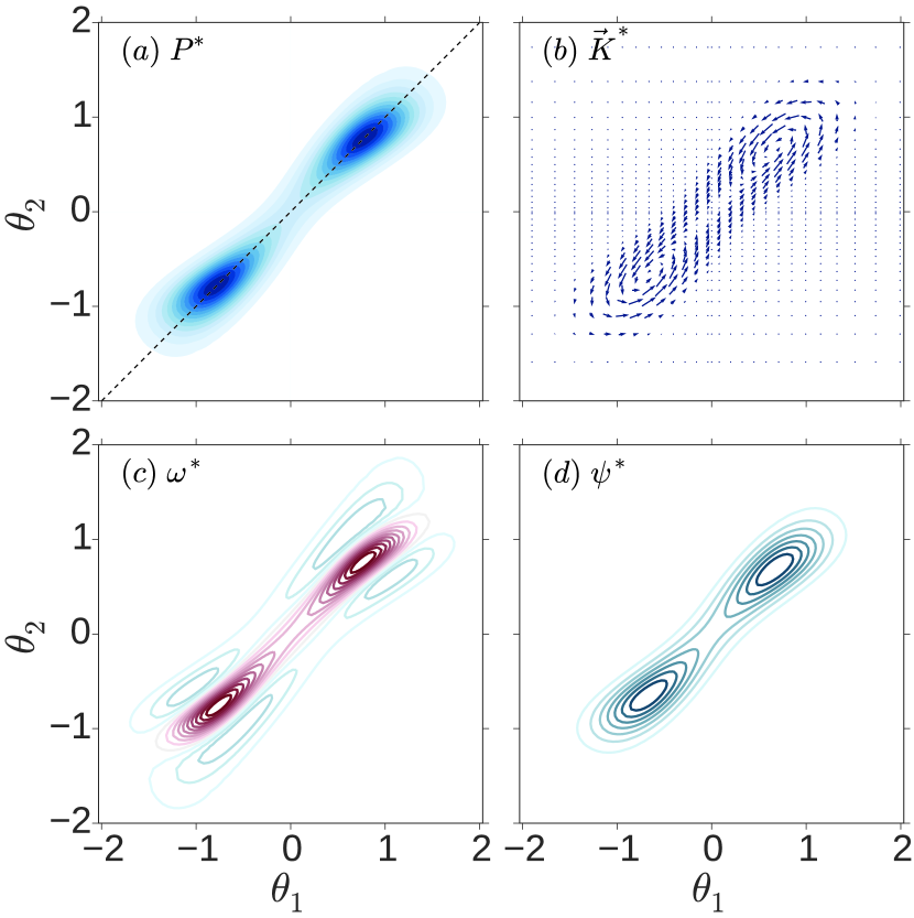
As briefly explained in Ref. Mellor et al. (2016a), the stationary distribution of the 2$q$VZ is characterized by two phases in general (as in the $q$VMZ Mobilia (2015)): When the fraction of zealots is low, the long-time opinion distribution $P^{\ast}$ is bimodal (low-zealotry phase) whereas it is single-peaked when the density of zealotry exceeds a critical value (high-zealotry phase). While this scenario will be scrutinized in the next sections, it is useful to gain some insight by considering some typical systems.

In many ways, the qualitative behavior of the 2$q$VZ resembles that of the mean-field version of the two-dimensional Ising model. The sum and difference, $\left(Z_{+}+Z_{-}\right)/N$ and $\left(Z_{+}-Z_{-}\right)/N$, play the role of temperature and external magnetic field, respectively. Thus, the transition in $P^{\ast}$ from displaying a single peak to being bimodal as zealotry is lowered. In the latter case, the two peaks are of equal height only when $Z_{+}=Z_{-}$ and the system exhibits criticality. Similar to the Ising model in a magnetic field, the 2$q$VZ is no longer critical when $Z_{+}\neq Z_{-}$ and the bimodal stationary probability is characterized by one peak that vanishes with the system size. While this phenomenology has also been observed in the $q$VMZ Mobilia (2015), the 2$q$VZ is genuinely out-of-equilibrium and it settles into a NESS whose quantitative features are shaped by non-trivial probability currents.

Using the methodology outlined above, we have explored the NESS of systems of various sizes up to $S_{1}\times S_{2}=100\times 100$. For the sake of illustration, we show typical results for $P^{\ast}$, $\vec{K}^{\ast}$, $\omega^{\ast}$, and $\psi^{\ast}$ in Fig. 3, for the low zealotry phase in the symmetric case $S_{1}=S_{2}=100$ and $Z_{\pm}=40$. Of course, the natural variables are just $n_{i}/S_{i}$, the fractions of each population holding opinion $+1$. On the other hand, there are some advantages to using a different set of variables: $\theta_{i}=\left(1/q_{i}\right)\ln{\left[(S_{i}/n_{i})-1\right]}$. First, the physical $\theta$’s occupy the entire plane, i.e., $\theta\in(-\infty,\infty)$, while the Ising-like symmetry of the 2$q$VZ corresponds to $\theta_{i}\leftrightarrow-\theta_{i}$. Second, the symmetry point $n_{i}=S_{i}/2$, is mapped to the origin. Finally, though there is no symmetry under the exchange of the two populations ($i=1\leftrightarrow 2$), we see that $P^{\ast}(\vec{\theta})$ is nearly symmetric under this reflection, see Fig. 3(a). In particular, as will be shown below, the fixed points of the deterministic mean-field rate equations (15), which correspond to the peaks of $P^{\ast}$, are situated on the $\theta_{1}=\theta_{2}$ line. Indeed, the “ridge” which runs from one peak through the saddle to the other is seen to lie very close to this line. In Fig. 3(b), we show the current field $\vec{K}^{\ast}$, which whirls around each peak of $P^{\ast}$. These whirls imply correlations of the dynamic properties of the two populations, indicating the tendency of $q_{2}$-voters to “follow” or “chase” $q_{1}$-voters Mellor et al. (2016a), a result that is corroborated by two-point correlation functions in Sec. IV.B. The bottom panels of Fig. 3 show the associated vorticity field and stream function. As expected, $\omega^{\ast}$ is positive near the peaks, corresponding to the current whirling counter-clockwise. Counter rotations ($\omega^{\ast}<0$) are present away from the peaks, a property not readily discerned when we examine the currents in Fig. 3(b). Lastly, we observe that the stream function $\psi^{\ast}$ appears to be very similar to $P^{\ast}$. This behavior is not a coincidence, as we will show that, in the linear Gaussian approximation, the two are strictly proportional to each other.

V Continuum Descriptions and Simulation Studies of Large Systems

As is often the case, the exact description of the 2$q$VZ through the master equation is intractable and difficult to analyze when the system size is large. Typically, Monte Carlo simulations are needed to explore their behavior. However, much insight can be gained through a continuum description and judicious approximations. Specifically, we consider the thermodynamic limit: $Z_{\pm},S_{i},N\rightarrow\infty$, with fixed densities $z_{\pm}=Z_{\pm}/N$ and $s_{i}=S_{i}/N$. In this limit, we expect demographic fluctuations to be negligible and the description in terms of mean-field rate equations is suitable. For large but finite systems, we can account for fluctuations and correlations via the Fokker-Planck equation (FPE) Van Kampen (1992); *gardiner1985handbook; *risken1984fokker associated with Eq. (1).

V.1 The Fokker-Planck Equation

When $N\gg 1$, the configuration space of densities $x_{i}=n_{i}/N$ approaches the continuum within a rectangle: $x_{i}\in\left[0,s_{i}\right]$, while time is rescaled so that $t=T/N$ is continuous. In other words, we will say that one Monte Carlo step (1 MCS) corresponds to $N$ moves of the microscopic model. Following standard procedures Lax (1966) to obtain the continuum limit of the ME (1), we arrive at the FPE for the probability density $P\left(\vec{x};t\right)$:

$$\frac{\partial}{\partial t}P\left(\vec{x};t\right)=\sum_{i=1,2}\frac{\partial}{\partial x_{i}}\left[\frac{\partial}{\partial x_{i}}u_{i}(\vec{x})P\left(\vec{x};t\right)-v_{i}(\vec{x})P\left(\vec{x};t\right)\right]$$ (12)

where $u_{i}\equiv\left(w_{i}^{+}+w_{i}^{-}\right)/2N$ and $v_{i}\equiv w_{i}^{+}-w_{i}^{-}$, and where $w_{i}^{+}=(s_{i}-x_{i})(z_{+}+x_{1}+x_{2})^{q_{i}}$ and $w_{i}^{-}=x_{i}(z_{+}+x_{1}+x_{2})^{q_{i}}$ are the continuum counterparts of $W_{i}^{\pm}$. The right-hand-side (RHS) can be identified as the divergence of the probability current density

$$K_{i}(\vec{x};t)=v_{i}P\left(\vec{x};t\right)-\partial_{i}\left[u_{i}P\left(\vec{x};t\right)\right]$$ (13)

where $\partial_{i}\equiv\partial/\partial x_{i}$. Clearly, in the NESS $P\left(\vec{x};t\right)\rightarrow P^{\ast}\left(\vec{x}\right)$, whereas the corresponding stationary probability current density is $K_{i}^{\ast}(\vec{x})=v_{i}P^{\ast}\left(\vec{x}\right)-\partial_{i}\left[u_{i}P^{\ast}\left(\vec{x}\right)\right]$. To find $P^{\ast}$, we must solve the partial differential equation $\sum_{i=1,2}\partial_{i}\left[\partial_{i}u_{i}(\vec{x})P^{\ast}\left(\vec{x}\right)-v_{i}(\vec{x})P^{\ast}\left(\vec{x}\right)\right]=0$ with non-trivial boundary conditions: vanishing of the normal components of $\vec{K}^{\ast}$. Thus, obtaining $P^{\ast}$ analytically in general is still quite challenging.

V.2 Mean-Field Analysis

A standard alternative to studying the FPE for the full distribution is to consider the equations governing the evolution of averages of various quantities Bogolubov and Gurov (1947); *yvon1935theorie. In particular, it is intuitively interesting to study the behavior of the average $\left\langle x_{i}\right\rangle_{t}\equiv\int x_{i}P\left(\vec{x};t\right)d\vec{x}$. Its evolution is governed by

$$\frac{d}{dt}\left\langle x_{i}\right\rangle=\int x_{i}\frac{\partial}{\partial t}P\left(\vec{x};t\right)d\vec{x}=\int K_{i}\left(\vec{x};t\right)d\vec{x}$$

since the surface contributions from the integration by parts involve the normal components of $\vec{K}$ and vanish. To make progress, we will need to make approximations. First, $\int\partial_{i}\left[u_{i}P\right]$ is also a surface term. Though it is not necessarily zero, it vanishes at the lowest order for large $N$. In this limit, we are left with contributions arising only from the first term on the right-hand-side of (13):

$$\frac{d}{dt}\left\langle x_{i}\right\rangle=\left\langle v_{i}\left(\vec{x}\right)\right\rangle$$

$$= \langle(s_{i}-x_{i})(z_{+}+x_{1}+x_{2})^{q_{i}}\rangle-\langle x_{i}(z_{+}+x_{1}+x_{2})^{q_{i}}\rangle.$$

Second, we invoke the mean-field approximation (MFA), which assumes that higher moments can be factored in terms of the averages $\langle x_{i}\rangle$ (e.g., $\left\langle x_{i}x_{j}\right\rangle\approx\left\langle x_{i}\right\rangle\left\langle x_{j}\right\rangle$). In this sense, the MFA neglects all correlations and fluctuations, an approach that becomes exact when $N\rightarrow\infty$. Within this approach, Eq. (V.2) becomes the mean-field rate equations (REs)   :

$$\frac{d}{dt}x_{i}=(s_{i}-x_{i})\mu^{q_{i}}-x_{i}(1-\mu)^{q_{i}}$$ (15)

where $\mu=z_{+}+x_{1}+x_{2}$ is the density of voters holding opinion $+$.

The fixed points (FPs) of these rate equations are stable or unstable nodes (no limit cycles in our case Mellor et al. (2016a, b)). They are given by

$$x_{i}^{\ast}=\frac{s_{i}}{1+\rho^{q_{i}}},$$ (16)

where $\rho=\left(1-\mu^{\ast}\right)/\mu^{\ast}$, with $\mu^{\ast}=z_{+}+x_{1}^{\ast}+x_{2}^{\ast}$. Note that $\rho$ is the ratio, in the steady state, of voters holding opinion $-$ to those with the $+$ opinion. It satisfies

$$\frac{1}{1+\rho}=z_{+}+\sum_{i=1,2}\frac{s_{i}}{1+\rho^{q_{i}}}$$ (17)

since the left hand side is $\mu^{\ast}=z_{+}+x_{1}^{\ast}+x_{2}^{\ast}$, which equals the right hand side. In terms of the variables $\theta_{i}$ introduced above, we recognize that $x_{i}=s_{i}/\left(1+e^{q_{i}\theta_{i}}\right)$, so that all FPs are given by $\theta_{i}^{\ast}=\ln\rho$.

We are particularly interested in the case $z_{+}=z_{-}=z$ for which the 2$q$VZ exhibits a continuous phase transition. In this case, it is clear that $\rho=1$ ($\mu^{\ast}=1/2$) is always a solution to Eq. (17), corresponding to the “central FP”: $\vec{x}^{\ast}=\vec{x}^{(0)}\equiv(s_{1}/2,s_{2}/2)$.The properties of this FP changes, as $z$ is decreased below a critical value $z_{c}$, from being stable to unstable. To show this property, we linearize Eq. (15) about a FP $\vec{x}^{\ast}$ and find the linear stability matrix, $-(\partial\dot{x_{i}}/\partial x_{j})|_{\vec{x}=\vec{x}^{\ast}}$, to have the form

$$\mathbb{F}(\vec{x}^{\ast})=\left(\begin{array}[]{cc}Y_{1\mu}-X_{1\mu}&-X_{1\mu}\\ -X_{2\mu}&Y_{2\mu}-X_{2\mu}\end{array}\right),$$ (18)

where

$$Y_{i\mu} = \mu^{\ast{q_{i}}}(1+\rho^{q_{i}}),$$

$$X_{i\mu} = {q_{i}}x_{i}^{\ast}(1-\mu^{\ast})^{{q_{i}-1}}\left(1+\rho\right).$$

Evaluating $\det{\mathbb{F}}$ at $\vec{x}^{\ast}={x^{(0)}}$, we find a remarkably simple result:

$$\det{\mathbb{F}(\vec{x}^{(0)})}=2^{2-q_{1}-q_{2}}\left[1-{q_{2}}s_{2}-{q_{1}}s_{1}\right]$$ (19)

Since a stable FP is associated with $\det{\mathbb{F}(\vec{x}^{(0)})}>0$, this expression implies that the 2$q$VZ resembles an Ising model at high temperatures when

$$1>s_{1}q_{1}+s_{2}q_{2}~{}~{}.$$ (20)

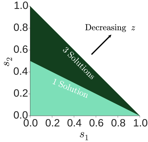
In the case $\det{\mathbb{F}(\vec{x}^{(0)})}<0$, ${\vec{x}^{(0)}}$ turns unstable and we can verify that there are two other (real $\rho$) solutions to Eq. (17), corresponding to two other stable, “non-central” FPs: $\vec{x}^{(\pm)}$ Of course, these correspond to the low temperature phase of the Ising model, with a spontaneously broken symmetry. Thus, we will refer to the line $s_{1}q_{1}+s_{2}q_{2}=1$ as the critical line (plotted in Fig. 4), separating the $s_{1}$-$s_{2}$ plane into a region where $\vec{x}^{(0)}$ is the sole FP and another where Eq. (15) admits three FPs. Before continuing, we emphasize that this technique is powerful enough for us to obtain the generalization of (20) to a population with any number of groups of $q_{i}$-voters, namely, $\vec{x}^{(0)}$ is stable when $1>\Sigma_{i}s_{i}q_{i}$. Details are given in Appendix C.

Since $1=2z+s_{1}+s_{2}$, we can express the critical $z_{c}$ as a function of the $q$’s and the difference $\Delta s\equiv s_{1}-s_{2}$

$$z_{c}=\frac{\bar{q}-1}{2\bar{q}}+\frac{q_{1}-q_{2}}{q_{1}+q_{2}}\frac{\Delta s}{2},$$ (21)

where $\bar{q}$ is the average $\left(q_{1}+q_{2}\right)/2$. In the limit of a homogeneous population ($q_{1}=q_{2}$), we recover the critical values $z_{c}=(q-1)/(2q)$ of the $q$VMZ Mobilia (2015). In this spirit, we may introduce an effective $q_{\text{eff}}$ for our heterogeneous $2q$VZ:

$$q_{\text{eff}}=\frac{s_{1}q_{1}+s_{2}q_{2}}{s_{1}+s_{2}}$$ (22)

in the sense that the number of FPs in the $2q$VZ are the same as those in the homogeneous $q$VMZ with this $q_{\text{eff}}$. Indeed, as shown in Appendix C, this notion can be generalized to $q_{\text{eff}}=\left.\left(\Sigma_{i}s_{i}q_{i}\right)\right/\left(\Sigma_{i}s_{i}\right)$ in the case of populations with any composition.

Figure 4: (Color online). Criticality in the $2q$VZ ($z_{\pm}=z$): Dependence of $z_{c}$ on the susceptible densities. Criticality at $z_{c}$ occurs on the interface between the blue/grey and green/black regions, prescribed by $s_{1}q_{1}+s_{2}q_{2}=1$, and the corresponding critical zealotry density is $z_{c}=(1-s_{1}-s_{2})/2$; see text. In the blue/grey region, the mean-field equations (15) have one fixed point, whereas they admit three fixed points in the green/black region; see text. Here, $(q_{1},q_{2})=(1,2)$.

V.3 Beyond MFA for Systems Far from Criticality

While the MFA provides an adequate picture of the deterministic aspects of the system’s evolution and the location of a phase transition, it cannot capture the stochastic nature of our model. In this section, we study the influence of demographic fluctuations in finite populations by means of the linear Gaussian approximation (LGA) of the FPE (12) Zia and Schmittmann (2007); Mellor et al. (2016a). To be concise, we focus on systems with symmetric zealotry ($z_{\pm}=z$) far from criticality, i.e., $z\ll z_{c}$ and $z\gg z_{c}$. In the realm of the LGA, we are able to compute many quantities of interest exactly, in the NESS. Beyond the LGA, we also study the mean switching time that characterizes the stochastic dynamics in the low zealotry phase when the system endlessly switches between the two stable fixed points $\vec{x}^{(\pm)}$.

V.3.1 Linear Gaussian Approximation of $P^{\ast}$

To describe fluctuations in the NESS, we examine the FPE (12) beyond the lowest order in $1/N$. This procedure can provide a scaling analysis of typical non-critical fluctuations in systems of large but finite size $N$. As our focus is the behavior in a NESS, we consider small deviations near a (stable) fixed point $\vec{x}^{\ast}$: $\vec{\xi}=\vec{x}-\vec{x}^{\ast}$. The LGA consists of linearizing the drift term of (12), i.e., $v_{i}\rightarrow(-\mathbb{F}\cdot\vec{\xi})_{i}$, while the diffusion coefficient is evaluated at $\vec{x}^{\ast}=(x_{1}^{\ast},x_{2}^{\ast})$, i.e., $u_{i}\rightarrow w_{i}^{\ast}=w_{i}^{+}(\vec{x}^{\ast})=w_{i}^{-}(\vec{x}^{\ast})$. Upon substitution into FPE (12), we obtain the LGA-FPE for the  stationary distribution:

$$0=\sum_{i,j=1,2}\frac{\partial}{\partial\xi_{i}}\left(\frac{\partial}{\partial\xi_{j}}D_{ij}+F_{ij}\xi_{j}\right)P^{\ast}(\vec{\xi}).$$ (23)

Here, $D_{ij}$ and $F_{ij}$ are the elements of the diffusion matrix $\mathbb{D}(\vec{x}^{\ast})$ and the drift matrix $\mathbb{F}(\vec{x}^{\ast})$, respectively. The former is given by

$$\mathbb{D}(\vec{x}^{\ast})=\frac{1}{N}\left(\begin{array}[]{cc}x_{1}^{\ast}(1-\mu^{\ast})^{q_{1}}&0\\ 0&x_{2}^{\ast}(1-\mu^{\ast})^{q_{2}}\end{array}\right)$$ (24)

(i.e., $D_{ij}=\delta_{ij}w_{i}^{\ast}/N$), while $\mathbb{F}$ is given by (18) . In general, the solution of (23) is still a Gaussian Lax (1966):

$$P^{\ast}(\vec{\xi})\propto\mathrm{exp}\left[-\frac{1}{2}\vec{\xi}\cdot\mathbb{C}^{-1}\vec{\xi}\right],$$ (25)

where $\mathbb{C}$ is the covariance matrix, with elements

$$C_{ij}=\langle\xi_{i}\xi_{j}\rangle^{\ast},$$ (26)

and can be obtained from $\mathbb{D}$ (24) and $\mathbb{F}$ (18) by solving $\mathbb{F}\mathbb{C}+\mathbb{C}\mathbb{F}^{T}=2\mathbb{D}$ Weiss (2003); *weiss2007fluctuation. Details, as well as the explicit forms for $\mathbb{C}$ in our case can be found in Appendix D. Since $\mathbb{D}$ is $O\left(1/N\right)$ and $\mathbb{F}$ is $O\left(1\right)$, it follows that $\mathbb{C}$ is also $O\left(1/N\right)$, confirming our expectation that the fluctuations (standard deviations) are $O\left(1/\sqrt{N}\right)$. Needless to say, if we approach criticality, then one of the eigenvalues of $\mathbb{F}$ approaches zero, so that $\mathbb{C}$ diverges and this approximation breaks down. On the other hand, for fixed $z\neq z_{c}$, the accuracy of the Gaussian expression (25) improves as $N\rightarrow\infty$. As an example of the quality of the LGA, we find that, for $N=400$ and $S_{i}=Z_{\pm}=100$, the prediction from (25) with (49) agrees with the numerically exact $P^{\ast}$ to $\lesssim$ $2\%$ within about two standard deviations.

V.3.2 Currents and correlations in the LGA

With a known $P^{\ast}$, we can find two exact expressions for the currents $\vec{K}^{\ast}=-\left\{\mathbb{D}\vec{\nabla}+\mathbb{F}\vec{\xi}\right\}P^{\ast}$. One displays the linear relationship $\vec{K}^{\ast}\propto\vec{\xi}P^{\ast}$:

$$\vec{K}^{\ast}(\vec{\xi})=\left\{\mathbb{D}\mathbb{C}^{-1}-\mathbb{F}\right\}\vec{\xi}P^{\ast}(\vec{\xi}).$$ (27)

The other shows explicitly that $\vec{K}^{\ast}$ is divergence free:

$$\vec{K}^{\ast}(\vec{\xi})=\frac{\mathbb{FC}-\mathbb{C}\mathbb{F}^{T}}{2}\vec{\nabla}P^{\ast}(\vec{\xi}),$$

where we have used $\mathbb{D=}\left[\mathbb{F}\mathbb{C}+\mathbb{C}\mathbb{F}^{T}\right]/2$. The key observation here is that the matrix is antisymmetric, which leads us to define

$$\mathbb{L}=\left(\begin{array}[]{cc}0&L_{12}\\ -L_{12}&0\end{array}\right)\equiv\mathbb{FC}-\mathbb{C}\mathbb{F}^{T}$$ (28)

In other words, $K_{i}^{\ast}=\varepsilon_{ij}\partial_{j}\left(L_{12}P^{\ast}/2\right)$, allowing us to identify the stream function $\psi^{\ast}=L_{12}P^{\ast}/2$, a linear relationship pointed out above. Further, from the continuum version of (10), we see that 

$$\left\langle\mathcal{L}\right\rangle^{\ast}=\int\varepsilon_{ij}\xi_{i}K_{j}^{\ast}d\vec{\xi}=L_{12}$$ (29)

Meanwhile, the vorticity field is proportional to $\xi_{i}\xi_{j}P^{\ast}$, so that it can be both positive and negative, as illustrated in Fig. 3(c).

Finally, we turn our attention to the continuum version of the general two point correlation, namely, $\langle\xi_{i}^{\prime}\xi_{j}\rangle_{\tau}^{\ast}=\int\xi_{i}^{\prime}\xi_{j}\mathcal{P}^{\ast}\left(\vec{\xi}^{\prime},\tau;\vec{\xi},0\right)d\vec{\xi}^{\prime}d\vec{\xi}$. In the LGA, it is much easier to use the solution to the corresponding Langevin equation Van Kampen (1992); *gardiner1985handbook; *risken1984fokker: $\vec{\xi}\left(\tau\right)=e^{-\mathbb{F}\tau}\vec{\xi}\left(0\right)$ plus noise. Since the noise is uncorrelated in time,

$$\left\langle\xi_{i}\left(0\right)\xi_{j}\left(\tau\right)\right\rangle^{\ast}=e^{-F_{jk}\tau}\left\langle\xi_{i}\left(0\right)\xi_{k}\left(0\right)\right\rangle^{\ast}=C_{ik}e^{-F_{jk}\tau}$$

The antisymmetric part of this correlation is necessarily odd in $\tau$ and does not vanish for systems in NESS. Also central to our study of NESS, we define the $t$-independent quantity Shkarayev and Zia (2014); Mellor et al. (2016a); Zia et al. (2016)

$$\widetilde{C}(\tau)\equiv\langle\xi_{1}(0)\xi_{2}(\tau)\rangle^{\ast}-\langle\xi_{2}(0)\xi_{1}(\tau)\rangle^{\ast}$$ (30)

which is the $12$ element of the matrix

$$\widetilde{\mathbb{C}}(\tau)=\mathbb{C}e^{-\mathbb{F}^{T}\tau}\mathbb{-}e^{-\mathbb{F}\tau}\mathbb{C}$$ (31)

Since $v_{i}\left(0\right)=\left.d\xi_{i}/d\tau\right|_{\tau=0}$, we see that the continuum version of (11) is $\left\langle\mathcal{L}\right\rangle^{\ast}=\left\langle\varepsilon_{ij}\xi_{i}v_{j}\right\rangle^{\ast}$, which implies

$$\left.\frac{d\widetilde{C}}{d\tau}\right|_{\tau=0}=\left\langle\mathcal{L}\right\rangle^{\ast};~{}~{}\left.\frac{d\widetilde{\mathbb{C}}}{d\tau}\right|_{\tau=0}=\mathbb{FC}-\mathbb{C}\mathbb{F}^{T}$$ (32)

within the LGA. Thus, we can regard $\widetilde{C}(\tau)$ as a generalized probability angular momentum, further details of which will be provided in the next subsection.

V.3.3 Simulation results for the symmetric case $s_{1,2}=s,z_{\pm}=1/2-s$

The above expressions (25)-(31) carry significant information on the NESS of the 2$q$VZ in the realm of the LGA and are valid for any values of $s_{1,2}$ and $q_{1,2}$. Here, we report the explicit results obtained for the symmetric case $s_{1,2}=s,z_{\pm}=\frac{1}{2}-s$ ($q_{2}=2q_{1}=2$). These results complete those in Ref. Mellor et al. (2016a) and allow us to discuss the validity of the LGA by considering a concrete example. Here, the explicit expressions of $C_{ij}$, the stationary correlation functions $\langle\xi_{i}\xi_{j}\rangle^{\ast}$, are given by (49) and (53), while the corresponding drift matrices $\mathbb{F}$ have been given in Ref. Mellor et al. (2016b) along with their (real and distinct) eigenvalues labeled by $\lambda_{\pm}$, where $\lambda_{+}>\lambda_{-}$.

To assess the validity of the LGA, we have performed Monte Carlo simulations of large systems with $N$ up to $14,400$, and compiled histograms from the trajectories to find the probability distribution $P^{\ast}(\vec{n})$. Similar to the comparison with the LGA prediction for smaller systems above, we find that (25) is an excellent approximation in the high-zealotry phase, i.e., $P^{*}(\vec{\xi})\simeq NP^{*}(\vec{n})$, with a sharp peak around the symmetric FP $\vec{x}^{(0)}$. In the low zealotry phase, we have confirmed that the stationary probability density is bimodal, with two sharp peaks close to the mean-field FPs $\vec{x}^{(\pm)}$. However, the distribution around each FP  is both skewed and more sharply peaked than the LGA prediction. For systems with $N\lesssim 10^{3}$ visible deviations between (25) and simulation results exist. Yet, for larger systems ($N\gg 10^{3}$), the agreements are quite reasonable, even in the low zealotry phase. We have confirmed this analysis by computing the skewness and (excess) kurtosis of in the 1D projections  of $P^{\ast}({\vec{\xi}})$ onto each axis in both regimes. For the smallest system we considered ($S=250$), in the low zealotry regime $Z=100$ the kurtosis was $(-0.242,0.750)$ for the $\xi_{1}$ and $\xi_{2}$ projections respectively. The skewness was $(0.321,0.969)$. For the high zealotry regime $Z=200$ the kurtosis was $(-0.030,-0.130)$ and skewness $(0.004,-0.007)$, confirming that the LGA is a better approximation at the high zealotry regime.

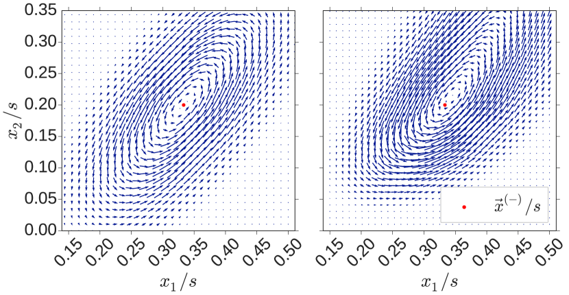
As the system size increases the kurtosis and skewness approach zero for both regimes. In Fig. 5, the LGA predictions (49) and (53) in the high/low zealotry phases are compared against the simulation results for $\langle\xi_{i}\xi_{j}\rangle^{\ast}$. The outcome confirms that $C_{ij}\propto 1/N$, i.e., fluctuations scale as $N^{-1/2}$, in both phases far from criticality. However, while the LGA provides a good quantitative predictions for $N\gtrsim 10^{3}$ in the $z>z_{c}$ cases, much larger system sizes ($N\gg 10^{3}$) are necessary to reach a similar quantitative agreement in the low-zealotry phase. We believe that the significant skewness associated with $\vec{x}^{(\pm)}$ in the latter regime when $N$ is not sufficiently large is responsible for the differences. A better and systematic understanding of this phenomenon is desirable, but beyond the scope of this study. Using Eq. (5), we can compute the probability current $\vec{K}^{\ast}$ exactly (for small systems) or via simulations and compare the results with the current obtained from Eq. (27) by using $P^{*}$ obtained within the realm LGA as shown in Fig. 6. From this comparison, we notice that due to finite size effects the MF fixed point and peaks of the distribution (around which $\vec{K}^{\ast}$ whirls) do not coincide perfectly, and the LGA flows are not symmetric around the fixed point. These discrepancies between simulations of the original 2$q$VZ and the LGA predictions are attenuated and eventually dissipate when the system size is increased. Furthermore, we also verified that, as predicted by the LGA, the stream function is always positive, in agreement with the counter-clockwise whirls of the probability current near the peaks reported in Fig. 3(b,c) and Fig. 6.

Figure 5: (Color online). $C_{ij}=\langle\xi_{i}\xi_{j}\rangle$ a function of system size $N$: Comparison of the LGA predictions (49) (left panel) and (53) (right panel) in solid against results of stochastic simulations (markers), averaged over at least $10^{5}$ MCS. The scaling $C_{ij}\propto 1/N$ is confirmed and the quantitative agreement improves as $N$ increases (with reasonably good agreement in the low-zealotry phase when $N\gg 10^{3}$). Here, $s_{1,2}=s$, $z_{\pm}=z=\frac{1}{2}-s$ with $q_{2}=2q_{1}=2$. In the two regimes $z>z_{c}$ and $z<z_{c}$ we have $z=2/9$ and $z=1/7$ respectively, the critical value being $z_{c}=1/6$.

Figure 6: (Color online). Stationary probability current: Comparison of the LGA predictions Eq. (27) (left panel) with the numerically exact counterpart Eq. (5) (right panel) near the fixed point $x^{(-)}$ (red/grey dot) in the low zealotry phase; see text. Parameters here are $(N,S_{1},S_{2},Z,q_{1},q_{2})=(280,100,100,40,1,2)$.

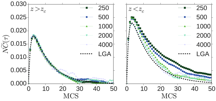
Turning to the antisymmetric two-point correlation function in the NESS $\widetilde{\mathbb{C}}(\tau)$, we find $\widetilde{C}(\tau)$ from the simulation trajectories $\vec{x}_{i}(t)$ via the lagged correlation: $\frac{1}{R-\tau}\sum_{t=0}^{R-\tau}\left[x_{1}(t)x_{2}(t+\tau)-x_{2}(t)x_{1}(t+\tau)\right]$, where $R$ is the length of our run (typically, $10^{5}$ MCS). From Eq. (31) we have

$$\widetilde{C}(\tau)=\langle\mathcal{L}\rangle^{\ast}\left(\frac{e^{-\lambda_{-}\tau}-e^{-\lambda_{+}\tau}}{\lambda_{+}-\lambda_{-}}\right)$$

where $\lambda_{\pm}$ are the eigenvalues of $\mathbb{F}$. In Fig. 7 we plot the LGA expression of $\widetilde{C}$ and the same quantity obtained from stochastic simulations and again find a good agreement in both high- and low-zealotry regimes. In particular, we notice that the LGA accurately captures the peak of $\widetilde{C}(\tau)$ at $\tau^{\ast}=[\ln{(\lambda_{+}/\lambda_{-})}]/[\lambda_{+}-\lambda_{-}]$ Mellor et al. (2016a). As illustrated in Fig. 7, the 2$q$VZ is characterized by $\widetilde{C}(\tau)>0$, i.e., $q_{i}$-susceptibles are correlated in such a way that $\langle x_{1}(t)x_{2}(t+\tau)\rangle^{\ast}>\langle x_{2}(t)x_{1}(t+\tau)\rangle^{\ast}$. This indicates that on a finite timescale (up to a separating time $\tau\approx 40-50$ in Fig. 7) $q_{2}$-voters are more likely to “follow” $q_{1}$-susceptibles than vice-versa. Clearly, for large lag times ($\tau\gg\lambda_{\pm}$), $\widetilde{C}\rightarrow 0$ and correlations are lost.

Figure 7: (Color online). LGA prediction of the two point correlation function, $\widetilde{C}(\tau)$ (dashed) compared to simulations (markers) in the high (left) and low (right) zealotry regimes for the symmetric case $s_{1,2}=s$, $z_{\pm}=z=\frac{1}{2}-s$ with $q_{1}=1$ and $q_{2}=2$. In the high zealotry regime, the LGA captures the behavior of $\widetilde{C}$ for all values of $S$ considered. For the low zealotry regime the LGA is qualitatively accurate for all $S$, however only quantitatively accurate for $S\geq 2000$. Fluctuations for MCS greater than $20$ are due to a low sampling rate. The LGA values for the peak $\tau^{\ast}$ for the high and low zealotry regimes, $2.80$ an $3.05$ respectively, accurately predict the data peak which occurs at $3$ in both cases.

V.4 Fluctuation Driven Dynamics below Criticality - Switching Times

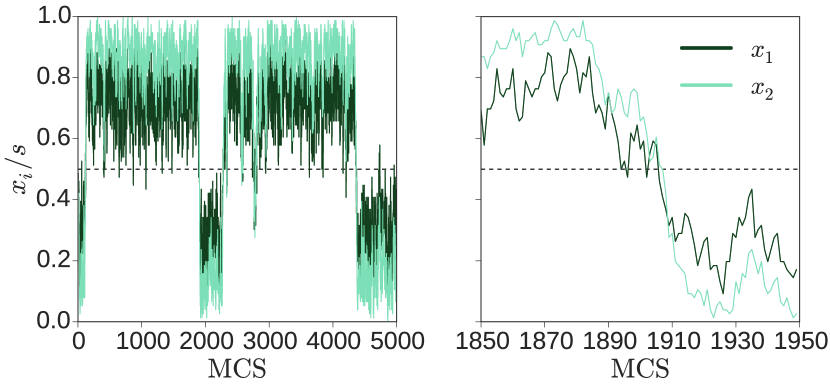
Similarly to what happens in the $q$VMZ Mobilia (2015) (see also Nyczka et al. (2012)), the long-time behavior in the low zealotry phase is characterized by a “swing-state dynamics”, or “switching dynamics” when there is the same number of zealots of both types or when there is only a small asymmetry in the zealotry. In the switching dynamics both the $q_{1}$- and $q_{2}$-susceptibles suddenly switch ‘almost’ simultaneously between the peaks $x_{i}^{(\pm)}\approx 0,s$ of $P^{*}(\vec{x})$, see Fig. 8. As explained above, $q_{2}$-voters “follow” $q_{1}$-voters and therefore $q_{1}$-susceptibles switch before $q_{2}$-susceptibles, however the lag between the switching of both populations is negligible in a first approximation, as shown in Fig. 8 (right), and will be neglected in what follows. In the remainder of this subsection, we focus on the case of symmetric zealotry, $z_{\pm}=z$.

This switching phenomenon that is driven by fluctuations, and therefore is beyond the reach of the mean-field analysis, can be analyzed in terms of the mean switching time $\tau_{s}$, measures the mean time to switch from one peak of $P^{*}(\vec{x})$, say $(x_{1}^{(-)},x_{2}^{(-)})$, to the other, $(x_{1}^{(+)},x_{2}^{(+)})$ for the first time Mobilia (2015).

Finding the mean switching time can be formulated as a first-passage problem whose solution, in terms of the FPE or the Kramer’s escape theory Eyring (1935); *kramers1940brownian; *hanggi1990reaction, is simple only in the single-variate case of a single type of susceptibles as in the $q$VMZ Mobilia (2015). However, as here the 2$q$VZ violates the detailed balance, the problem is much more complicated.

Figure 8: (Color online). Switching behavior of the $2q$VZ at $z<z_{c}$: Time series for the total density of $+1$ susceptible voters within each population ($x_{i}/s_{i}$). Sample of $5000$ MCS (left) and closer examination of a typical switching period (right). One unit of time $t=\tau/N$ is $1$ MCS and equates to $N$ iterations of the model. Here parameters are: $(N,s_{1},s_{2},z,q_{1},q_{2})=(200,0.38,0.38,0.12,1,2)$.

Figure 9: (Color online). Mean switching time $\tau_{s}$ between the two stable fixed points for systems of size $N=100$ with $(q_{1},q_{2})=(1,2)$. Results obtained from stochastic simulations (green/black $\square$ with dotted line) are compared with the approximation 33 (blue/grey solid line); see text. Simulation data are averaged over $10^{6}$ MCS. Here $s_{1,2}=s=\frac{1}{2}-z$.

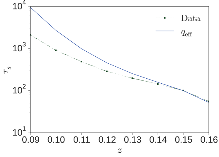
An approximation of $\tau_{s}$ is obtained by exploiting the mapping onto the $q$VMZ for values of $z$ just below the critical value $z_{c}$ ($z\lesssim z_{c}$). In this regime, we expect that the switching dynamics of the 2$q$VZ with $(q_{1},q_{2})$ can be approximately mapped onto that of the $q$VMZ with an effective value $q_{\mathrm{eff}}$ given by (22). In this approximation the mean switching time between the two fixed points of the qVMZ, $x^{(\pm)}$, can be computed as in in Ref. Mobilia (2015) by solving $\mathcal{G}_{b}^{\mathrm{eff}}(x)\tau_{s}(x)=-1$ with the reflective and absorbing conditions $(d/dx)\tau_{s}(x^{(-)})=\tau_{s}(x^{(+)})=0$, which yields

$$\tau_{s}=2N\int_{x^{(-)}}^{x^{(+)}}dye^{-N\phi(y)}\int_{x^{(-)}}^{y}\frac{e^{N\phi(v)}dv}{\tilde{w}^{+}(v)+\tilde{w}^{-}(v)},$$ (33)

where $\phi(v)=2\int_{x^{(-)}}^{v}\left\{\frac{\tilde{w}^{+}(v)-\tilde{w}^{-}(v)}{\tilde{w}^{+}(v)+\tilde{w}^{-}(v)}\right\}$. Now, $\tilde{w}^{+}(x)=(s_{1}+s_{2}-x)(x+z)^{q_{\mathrm{eff}}}$ and $\tilde{w}^{-}(x)=x(s_{1}+s_{2}+z-x)^{q_{\mathrm{eff}}}$ and therefore, using the Kramers’ formula Eyring (1935); *kramers1940brownian; *hanggi1990reaction; Mobilia (2015), we have

$$\ln{\tau_{s}}\simeq 2N\int_{x^{(-)}}^{x_{1}^{(+)}}\frac{\tilde{w}^{-}(y)-\tilde{w}^{+}(y)}{\tilde{w}^{-}(x^{(-)})+\tilde{w}^{+}(x^{(-)})}~{}dy$$ (34)

which predicts that the mean switching time $\tau_{s}$ grows (approximately) exponentially with $N$ Mobilia (2015) The results reported in Fig. 9 confirm that this approximation is accurate just below $z_{c}$, while it overestimates $\tau_{s}$ at lower values of $z$. The fact that the mean switching time in the 2$q$VZ is generally shorter than in its equilibrium $q$VMZ (with $q=q_{\mathrm{eff}}$) counterpart suggests that the probability currents, absent in the $q$VMZ, are responsible for speeding up the switching dynamics by reducing the switching time.

V.5 Behavior Near Criticality

Up to now, we have mostly focused on the properties on the 2$q$VZ deep in the high-zealotry and low-zealotry phases. Here we focus on some properties of the system close to criticality: $z_{\pm}=z\approx z_{c}$.

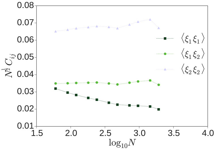
Since, every individual in our system is connected to every other (i.e., a complete graph), we anticipate that a Landau-like description should be adequate to capture the critical behavior. Specifically, we are concerned with how the fluctuations (co-variances $C_{ij}$) scale with $N$ at criticality. By formal analogy with the standard approach for an Ising magnet, we consider a free energy functional (at zero external magnetic field) Goldenfeld (1992); *tauber2014critical.

$$\mathcal{F}\left(m\right)=N\left\{\frac{rm^{2}}{2}+\frac{gm^{4}}{4}\right\}$$

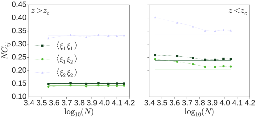
where $r$ is a measure of the deviation from the critical point (e.g., $T-T_{c}$) and $g>0$. Thus, using $P\left(m\right)\propto e^{-\mathcal{F}}$, we find $\left\langle m^{2}\right\rangle\propto N^{-1}$ and $N^{0}$, above and below criticality respectively - as reported in the previous section. For $r=0$, however, $\left\langle m^{2}\right\rangle\propto N^{-1/2}$. In Fig. 10, we report that in line with the above general considerations all three stationary two-point correlation functions $\langle\xi_{i}\xi_{j}\rangle$ of the 2$q$VZ measured from simulations with $z=z_{c}$ indeed approach this behavior as $N$ increases: $\langle\xi_{i}\xi_{j}\rangle\sim N^{-1/2}$.

A full finite-size-scaling analysis of the entire critical region should include (i) the behavior of $z_{c}$ as a function of $N$, (ii) the effects of $z_{+}\neq z_{-}$, (iii) the Binder cumulant (excess kurtosis), etc. We fully expect universal behavior, i.e., properties which do not depend on the detailed partition into the two populations ($s_{1},s_{2}$). While valuable, such a study is beyond the scope of this paper.

Figure 10: (Color online). Correlations as a function of system size $\log_{10}(N)$ for simulated results, averaged over at least $10^{5}$ MCS. The fluctuations roughly scale as $N^{-1/2}$ as predicted. Here the parameters are: $(s_{1},s_{2},z,q_{1},q_{2})=(\frac{1}{3},\frac{1}{3},\frac{1}{6},1,2)$. $N$ varies from $N=60$ to $1920$.

VI The 2$q$VZ with Asymmetric Zealotry

In this section we briefly outline the main properties of the 2$q$VZ with asymmetric zealotry by assuming that, say, $Z_{+}>Z_{-}$.

The 2$q$VZ with asymmetric zealotry shares qualitatively the same features as its $q$VMZ counterpart Mobilia (2015): It also displays a high- and low-zealotry phase which are respectively characterized by a unimodal and bimodal stationary probability distribution $P^{*}$. However, the latter are now no longer symmetric: in the low-zealotry phase the peak associated with the opinion supported by $Z_{+}$ zealots is much more pronounced than that associated with $Z_{-}$ zealots (see Fig. 11(left)), whereas the single-peaked distribution in the high-zealotry phase is skewed towards states with a majority of $+1$ voters. When $N$ is sufficiently large, the peaks of $P^{*}$ of course correspond to the fixed points of the mean-field equation (15) whose analysis reveals that, as for the $q$VMZ, in the low-zealotry phase the two stable fixed points $\vec{x}^{(\pm)}$ are separated by the unstable steady state $\vec{x}^{(0)}$, while in the high-zealotry phase only $\vec{x}^{(+)}$ is stable. However, again, a major difference between the 2$q$VZ and the $q$VMZ is that the former violates the detailed balance which results in the steady state being a NESS and in a number of intriguing results such as the existence of stationary current of probability that form closed loops in the configuration space. A typical example of the exact NESS probability distribution $P^{*}$ in the low zealotry phase with $Z_{+}>Z_{-}$ is shown in Fig. 11 along with the wind field of the stationary probability current $\vec{K}^{*}$.

Figure 11: (Color online). Numerically exact NESS probability distribution $P^{*}$ and probability current $\vec{K}^{*}$ in the low-zealotry phase with asymmetric zealotry: (Left) Darkness indicate regions in the $x_{1}/s-x_{2}/s$ where $P^{*}$ is high ($P^{*}$ being higher where it is darker). (Right) Vector field of the probability current $\vec{K}^{*}$. Parameters are: $(N,S_{1},S_{2},Z_{+},Z_{-},q_{1},q_{2})=(258,100,100,30,28,1,2)$.

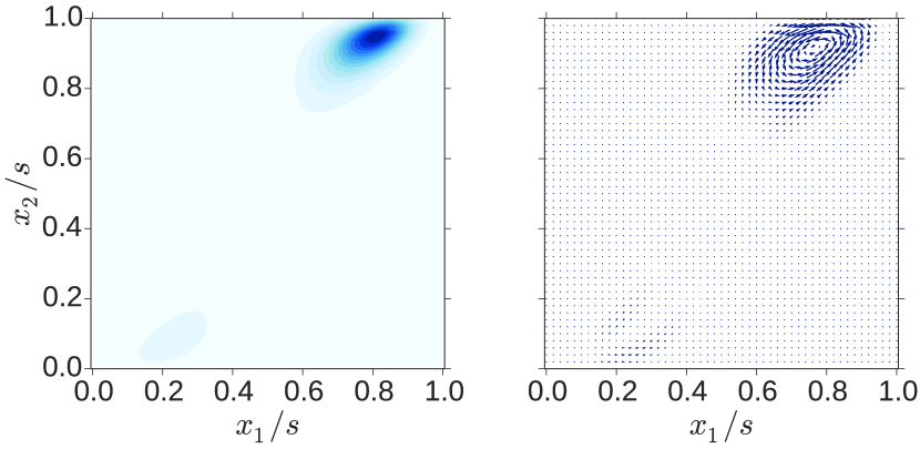
In Fig. 11(left), we see that even when there is a small asymmetry in the zealotry the peak corresponding to $\vec{x}^{(-)}$ is almost invisible and the distribution is dominated by the peak associated with $\vec{x}^{(+)}$ and whose intensity increases with $N$. As a consequence, the stationary probability current $\vec{K}^{*}$ flows mostly around $\vec{x}^{(+)}$ in an anti-clockwise fashion (vorticity is positive), even though there is current flow around $\vec{x}^{(-)}$ but with a much smaller amplitude. These features of the 2$q$VZ with asymmetric zealotry can be analyzed using the techniques of Sec. IV and more specifically the Fokker-Planck and linear Gaussian approximations in the continuum limit when $N\gg 1$. In fact, we can still use (25)-(31) within the LGA and obtain the stationary probability density $P^{*}(\vec{\xi})$ near the fixed points in each of the phase, as well as the LGA expressions of the stationary density current $\vec{K}^{*}(\vec{\xi})$, correlation functions $C_{ij}=\langle\xi_{i}\xi_{j}\rangle$ and $\widetilde{C}(t)$, vorticity and average probability angular momentum $\langle\mathcal{L}\rangle^{\ast}$. Since the bimodal probability density $P^{*}(\vec{\xi})$ is dominated by the peak $\vec{x}^{(+)}$ in the low-zealotry phase, the LGA is expected to work even better when the zealotry is asymmetric since the skewness that characterizes $P^{*}(\vec{\xi})$ in this regime disappears when $N$ is large enough.

Figure 12: (Color online). Metastability and switching dynamics in the low-zealotry phase with asymmetric zealotry: Shown is the first $10^{4}$ MCS of a typical single realization with initial condition $\vec{x}=(0,0)$ and switching occurring around $t\approx 1000$. Parameters are: $(N,S_{1},S_{2},Z_{+},Z_{-},q_{1},q_{2})=(258,100,100,30,28,1,2)$.

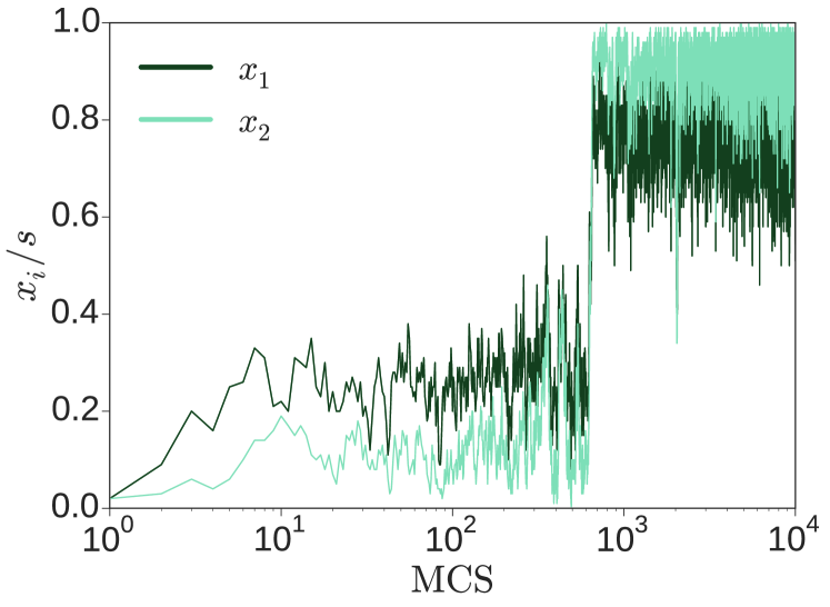
When the zealotry is asymmetric the long-time dynamics is characterized by metastability: While in principle chance fluctuations can cause the continuous switching of susceptibles population from the (metastable state) $\vec{x}^{(-)}$ into the state $\vec{x}^{(+)}$ and vice versa, owed to the asymmetry in $P^{*}$ only the switch from $\vec{x}^{(-)}$ to $\vec{x}^{(+)}$ is observable in practice (when $Z_{+}>Z_{-}$), as in the $q$VMZ Mobilia (2015). This phenomenon is associated with the metastability of the fixed points $\vec{x}^{(\pm)}$ and as such is triggered by a rare large fluctuation: As shown in Fig. 12, a chance fluctuation causes the sudden and almost simultaneous switch of both $q_{i}$-subpopulations from $\vec{x}^{(-)}$ to $\vec{x}^{(+)}$. In a large population, the system settles in the new metastable and fluctuates in its vicinity but cannot be observed to switch back to $\vec{x}^{(-)}$. The mean time for the transition $\vec{x}^{(-)}$ to $\vec{x}^{(+)}$ can be estimated by using the same approach as in the case of symmetric zealotry and also gives a mean time that grows exponentially with the population size, which is typical of a system characterized by metastability.

VII Discussion and Conclusion

This work has been dedicated to the detailed analysis of a heterogeneous out-of-equilibrium nonlinear voter model in a finite well-mixed population. More specifically, we have carefully analyzed the properties of 2$q$VZ model that we introduced in Ref. Mellor et al. (2016a) where two types of swing voters need the consensus of $q_{1}$ or $q_{2}(\neq q_{1})$ of their neighbors to adopt their opinion and are influenced by the presence of zealots. The 2$q$VZ is a direct but non-trivial generalization of the $q$-voter model with zealots ($q$VMZ) Mobilia (2015). Both models mimic important concepts of social psychology and sociology, such as the relevance group-size on the mechanism of conformity for collective actions, and the interplay between independence and conformity. However, from a mathematical viewpoint the 2$q$VZ strikingly differs from the $q$VMZ by violating the detailed balance and is therefore genuinely out of equilibrium. Many of the qualitative features of the 2$q$VZ are similar to those displayed by the $q$VMZ: When the zealotry density is low, the long-time opinion distribution is bimodal whereas it is single-peaked at high zealotry. Furthermore, the 2$q$VZ is also characterized by a switching dynamics when there is an equal number of zealots of both types and by metastability when there is an asymmetry in the zealotry. However, the non-equilibrium nature of the 2$q$VZ has far-reaching consequences that we have investigated in detail. In particular, we have characterized the system’s non-equilibrium steady state (NESS) in terms of its probability distribution and probability currents that form closed loops in the state space, as well as the unequal-time correlation functions to highlight the violation of the time-reversal. These quantities have been computed numerically exactly for small systems and by means of stochastic simulations in larger populations. Furthermore, we have also investigated these quantities analytically in the realm of the linear Gaussian approximation (LGA) obtained in the limit of large systems and far from the criticality. We have also focused on the long-time switching dynamics of the 2$q$VZ in the low-zealotry phase and have devised an approximation by mapping the mean switching time of the 2$q$VZ on that computed in Ref. Mobilia (2015) for the $q$VMZ. We have also studied some properties of these systems at criticality and outlined the behavior of the 2$q$VZ when the zealotry is asymmetric.

This work has allowed us to draw a comprehensive picture of the various properties of the 2$q$VZ and of the consequences of the violation of the detailed balance and we have shown that LGA is a particularly useful method. It shall be interesting to investigate this model on complex and/or adaptive networks that would be relevant from a social dynamics perspective. An intriguing question is the macroscopic interpretation of the closed loops of probability current: can these be related to the presence of “leaders” and “followers” in a society?

VIII Acknowledgements

We are grateful to J. Knebel for a critical reading of the manuscript and useful suggestions. We thank K. E. Bassler, B. Schmittmann and J. B. Weiss for enlightening discussions. This work was supported by an EPSRC Industrial Case Studentship Grant No. EP/L50550X/1. Partial funding from Bloom Agency in Leeds U.K. is also gratefully acknowledged. This research was supported partly by US National Science Foundation Grants No. OCE-1245944 and No. DMR-1507371. One of us (R.K.P.Z.) is grateful for the hospitality of the Leeds School of Mathematics, as well as financial support from the LSM and the London Mathematical Society (Grant No. 41517). M.M. is grateful for the hospitality of the LSFrey at the Arnold Sommerfeld Center (University of Munich), as well as for the financial support of the Alexander von Humboldt Foundation (Grant No. GBR/1119205).

Appendix A Master Equation and Probability Currents

In this appendix, we outline how the probability current is obtained from the master equation (ME) characterizing the evolution of a generic interacting stochastic process. For simplicity, let us focus on a system with configuration space $\left\{\mathcal{C}\right\}$, evolving in discrete time steps. Suppressing the reference to the initial configuration, $\mathcal{C}_{0}$, we consider the evolution of $P\left(\mathcal{C},t\right)$, the probability to find the system in the configuration $\mathcal{C}$ at time $t$. In a general Markov chain with finite state space, this evolution is specified by only the probabilities for the system to transition from configuration $\mathcal{C}$ to $\mathcal{C}^{\prime}$ in one time step: $W\left(\mathcal{C}\rightarrow\mathcal{C}^{\prime}\right)$. The ME for $P\left(\mathcal{C},t\right)$ can be written as

$$P\left(\mathcal{C}^{\prime},t+1\right)=\sum_{\mathcal{C}}\mathcal{G}\left(\mathcal{C}^{\prime},\mathcal{C}\right)P\left(\mathcal{C},t\right),$$ (35)

where the evolution operator $\mathcal{G}$ thus reads

$$\mathcal{G}\left(\mathcal{C}^{\prime},\mathcal{C}\right)=\delta\left(\mathcal{C}^{\prime},\mathcal{C}\right)\left[1-\sum_{\mathcal{C}^{\prime\prime}}W\left(\mathcal{C\rightarrow C}^{\prime\prime}\right)\right]+W\left(\mathcal{C}\rightarrow\mathcal{C}^{\prime}\right),$$ (36)

where $\delta$ is the Kronecker delta. Clearly, we can regard $P$ as a vector and $\mathcal{G}$ as a (stochastic) matrix, generating a new vector at each time step. The change in $P\left(\mathcal{C},t\right)$ can be regarded as a sum over probability currents into and out-of $\mathcal{C}$. Specifically, the net current from $\mathcal{C}$ to $\mathcal{C}^{\prime}$ is given by

$$K\left(\mathcal{C}\rightarrow\mathcal{C}^{\prime},t\right)=W\left(\mathcal{C}\rightarrow\mathcal{C}^{\prime}\right)P\left(\mathcal{C},t\right)-W\left(\mathcal{C}^{\prime}\rightarrow\mathcal{C}\right)P\left(\mathcal{C}^{\prime},t\right)$$ (37)

so that

$$P\left(\mathcal{C},t+1\right)-P\left(\mathcal{C},t\right)=-\sum_{\mathcal{C}^{\prime}}K\left(\mathcal{C}\rightarrow\mathcal{C}^{\prime},t\right)$$ (38)

takes the form of a discrete continuity equation. Much is know about stochastic matrices of the form $\mathcal{G}$. In particular, its largest eigenvalue is unity and there is (at least) one associated eigenvector, which can be identified with the stationary state, $P^{\ast}\left(\mathcal{C}\right)$. Further, if the dynamics is ergodic (all $\mathcal{C}$’s can be reached from any $\mathcal{C}_{0}$ with the $W$’s), then $P^{\ast}$ is unique.

Beyond probabilities at one time, we can consider joint distributions, with the system evolving from $t$ to a later time $t+\tau$:

$$\mathcal{P}\left(\mathcal{C}^{\prime},t+\tau;\mathcal{C},t\right)=\mathcal{G}^{\tau}\left(\mathcal{C}^{\prime},\mathcal{C}\right)P\left(\mathcal{C},t\right)$$ (39)

where $\mathcal{G}^{\tau}$ is the matrix product of $\mathcal{G}$ with itself, $\tau$ times.

If detailed balance is satisfied (i.e., if $W$’s satisfy the Kolmogorov criterion Kolmogorov (1936)), then all currents in the stationary state

$$K^{\ast}\left(\mathcal{C}\rightarrow\mathcal{C}^{\prime}\right)=W\left(\mathcal{C}\rightarrow\mathcal{C}^{\prime}\right)P^{\ast}\left(\mathcal{C}\right)-W\left(\mathcal{C}^{\prime}\rightarrow\mathcal{C}\right)P^{\ast}\left(\mathcal{C}^{\prime}\right)$$ (40)

vanish, yielding $K^{\ast}=0$. When detailed balance is violated, then the stationary state is a NESS and some $K^{\ast}$ will be non-vanishing. Stationarity implies that currents $K^{\ast}$ are “divergence” free, i.e., $\sum_{\mathcal{C}^{\prime}}K^{\ast}\left(\mathcal{C}\rightarrow\mathcal{C}^{\prime}\right)=0$. This means that $K^{\ast}$ must be the ‘curl’ of a certain quantity, while its ‘curl’ generally does not vanish. In other words, the currents form closed loops in $\mathcal{C}$ space. By analogy with the current $\vec{J}$ in classical mechanics of incompressible fluids (where $\vec{\nabla}\cdot\vec{J}=0$), these current loops lead us to other concepts, notably the vorticity field ($\vec{\omega}=\vec{\nabla}\times\vec{J}$), the stream function ($\vec{J}=\vec{\nabla}\times\vec{\psi}$), and total angular momentum ($\int_{\vec{r}}\vec{r}\times\vec{J}$).

A.1 Probability Current and Observables in the 2$q$VZ

Here, we study discrete version of these quantities in a very simple configuration space: In the 2$q$VZ, the $\mathcal{C}$ space is just the set of integer points $\left(n_{1},n_{2}\right)\in S_{1}\times S_{2}$. With (II.1), the evolution operator of the 2$q$VZ is given by (II.1). Hence, with (37) and (II.1), the probability net current associated in the 2$q$VZ is given by

$$K_{1}(\vec{n};t) = W_{1}^{+}(\vec{n})P\left(\vec{n};t\right)$$

$$- W_{1}^{-}(\vec{n}+\vec{e}_{1})P\left(\vec{n}+\vec{e}_{1};t\right)$$

$$K_{2}(\vec{n};t) = W_{2}^{+}(\vec{n})P\left(\vec{n};t\right)$$ (41)

$$- W_{2}^{-}(\vec{n}+\vec{e}_{2})P\left(\vec{n}+\vec{e}_{2};t\right).$$

In the continuum limit, $\vec{n}/N\rightarrow\vec{x}$, the usual notation of divergence and curl applies. Meanwhile, $\vec{K}^{\ast}\left(\vec{x}\right)=(K_{1}^{\ast}\left(\vec{x}\right),K_{2}^{\ast}\left(\vec{x}\right))$ is a two component vector field while both the vorticity and stream function are scalar fields:

$$\omega^{\ast}\left(\vec{x}\right)=\varepsilon_{ij}\frac{\partial K_{j}^{\ast}\left(\vec{x}\right)}{\partial x_{i}};~{}~{}K_{i}^{\ast}\left(\vec{x}\right)=\varepsilon_{ij}\frac{\partial\psi\left(\vec{x}\right)}{\partial x_{j}}$$ (42)

where $\varepsilon_{ij}$ is the two-dimensional Levi-Civita symbol and repeated indices are summed. The interpretation of these quantities is the following: Vorticity $\omega^{\ast}$ represents the ‘essence’ or ‘source’ of $\vec{K}^{\ast}$, much like electric currents are the sources of magnetic field. On the other hand, $\vec{K}^{\ast}$ is just a $90^{\circ}$ rotation of $\vec{\nabla}\psi^{\ast}$ and $\psi^{\ast}$ therefore provides a simple way to visualize the probability current.

Since it is generally difficult to visualize probability currents, it is also useful to introduce a quantity $L_{ij}$, which is the (average) “probability angular momentum” Shkarayev and Zia (2014); Mellor et al. (2016a) and the formal analog of the total angular momentum of a fluid:

$$L_{ij}=\int_{\vec{x}}\varepsilon_{ij}x_{i}K_{j}^{\ast}(\vec{x})~{}d{\vec{x}}=\int_{\vec{x}}\left[x_{i}K_{j}^{\ast}(\vec{x})-x_{j}K_{i}^{\ast}(\vec{x})\right]~{}d{\vec{x}},$$ (43)

where $i,j\in(1,2)$. The probability angular momentum has a single independent component, say $L_{12}=-L_{21}=\langle\mathcal{L}\rangle^{\ast}$. Since, $\vec{K}^{\ast}$ is divergence-free ($\partial K_{i}/\partial x_{i}=0$), $\langle\mathcal{L}\rangle^{\ast}$ is independent of the choice of the origin of $\left\{\vec{x}\right\}$.

We are particularly interested in the average number of $q_{i}$-susceptibles and their two-point correlation function in the NESS of the 2$q$VZ, which read:

$$\langle n_{i}\rangle^{*} = \sum_{\vec{n}}n_{i}P^{\ast}(\vec{n}),$$

$$\langle n_{i}^{\prime}n_{j}\rangle^{*}_{T} = \sum_{\vec{n},\vec{n}^{\prime}}n_{i}^{\prime}n_{j}\mathcal{P}^{*}(\vec{n},T;\vec{n}^{\prime},0).$$ (44)

In particular, the lagged correlation $C_{ij}(\tau)=\langle x_{i}^{\prime}x_{j}\rangle_{N\tau}=\langle n_{i}^{\prime}n_{j}\rangle_{T}/N^{2}$, is directly related to $\langle\mathcal{L}\rangle^{\ast}$ (43) when $T=1$. In fact, in continuous time $\tau\to t=T/N$, the average probability angular momentum $\langle\mathcal{L}\rangle^{\ast}$ is the antisymmetric part $\widetilde{C}_{ij}=C_{ij}-C_{ji}$ of this two-point unequal-time correlation function in the NESS Mellor et al. (2016a): $\langle\mathcal{L}\rangle^{*}=\left.\partial_{\tau}\widetilde{C}(\tau)\right|_{0}$; see Eq. (32).

The proof for $\left\langle\mathcal{L}\right\rangle^{\ast}=\left\langle\vec{n}\times\left(\vec{W}^{+}-\vec{W}^{-}\right)\right\rangle$ in NESS starts with

$$\left\langle\mathcal{L}\right\rangle^{\ast}=\sum_{\vec{n}}n_{1}K_{2}^{\ast}\left(\vec{n}\right)-n_{2}K_{1}^{\ast}\left(\vec{n}\right)$$

and substituting in the expression for stationary flows (5). Rearranging various terms on the RHS we have

$$= \phantom{+}\sum_{\vec{n}}\left[n_{1}W_{2}^{+}(\vec{n})-n_{2}W_{1}^{+}(\vec{n})\right]P^{\ast}(\vec{n})$$

$$-\sum_{\vec{n}}n_{1}W_{2}^{-}(\vec{n}+\vec{e}_{2})P^{\ast}(\vec{n}+\vec{e}_{2})$$

$$+\sum_{\vec{n}}n_{2}W_{1}^{-}(\vec{n}+\vec{e}_{1})P^{\ast}(\vec{n}+\vec{e}_{1})$$

$$= \phantom{+}\sum_{n_{1},n_{2}=0}n_{1}W_{2}^{+}(n_{1},n_{2})P^{\ast}(n_{1},n_{2})$$

$$-\sum_{n_{1},n_{2}=0}n_{2}W_{1}^{+}(n_{1},n_{2})P^{\ast}(n_{1},n_{2})$$

$$+\sum_{n_{1}=1,n_{2}=0}n_{2}W_{1}^{-}(n_{1},n_{2})P^{\ast}(n_{1},n_{2})$$

$$-\sum_{n_{1}=0,n_{2}=1}n_{1}W_{2}^{-}(n_{1},n_{2})P^{\ast}(n_{1},n_{2})$$

where $\sum_{n_{1},n_{2}=0}$ is the sum over both indices, starting at $0$. For the last two terms, we can sum over $n_{i}^{\prime}=n_{i}+1$ starting at $n_{i}^{\prime}=1$. But, since

$$W_{1}^{-}(0,n_{2})=0=W_{2}^{-}(n_{1},0)$$

this sum can be extended to $n_{i}^{\prime}\in\left[0,S_{i}\right]$.

$$= \phantom{+}\sum_{n_{1},n_{2}=0}\left[n_{1}W_{2}^{+}(n_{1},n_{2})-n_{2}W_{1}^{+}(n_{1},n_{2})\right]P^{\ast}(n_{1},n_{2})$$

$$+\sum_{n_{1},n_{2}=0}\left[n_{2}W_{1}^{-}(n_{1},n_{2})-n_{1}W_{2}^{-}(n_{1},n_{2})\right]P^{\ast}(n_{1},n_{2})$$

Combining everything, we have

$$\left\langle\mathcal{L}\right\rangle^{\ast}=\sum_{\vec{n}}\left[n_{1}\left(W_{2}^{+}-W_{2}^{-}\right)-n_{2}\left(W_{1}^{+}-W_{1}^{-}\right)\right]P^{\ast}.$$

Appendix B Calculating $P^{*}$ for large systems

For small systems, the full master equation is solvable numerically to find the stationary state $P^{*}(\vec{n})$, and subsequently the stationary currents $\vec{K}^{*}$. This is very useful for assisting in the understanding of the model. However this approach is problematic in that the number of non-zero entries in powers of the transition matrix $\mathcal{G}=[{\cal G}(\vec{n^{\prime}},\vec{n})]$ grows approximately quadratically with the power. As there are $(S_{1}+1)\times(S_{2}+1)$ possible states, the transition matrix has $(S_{1}+1)^{2}(S_{2}+1)^{2}$ entries. For a systems with $S=(S_{1}+S_{2})/2>100$, storing these transition matrices fully in memory becomes non-trivial. For $S=300$, the required memory is $65$GB (with double precision) which is far beyond the realms of standard computer setups.

Thankfully it is possible to attain the stationary distribution for larger systems relatively quickly, managing a trade-off between computational intensity and memory. After computing the stationary distribution of a smaller system exactly we use linear interpolation to approximate the stationary distribution, $\tilde{P}^{\ast}(\vec{x})$, of a system which is a factor $r$ larger (or a factor $r$ more granular when considering the densities). In particular, for $r=2$, we begin with

$$\tilde{P}^{\ast}(\vec{x})=P^{\ast}(\vec{x})$$

for $x_{i}=n_{i}/N$ (and so $x_{i}=2n_{i}/2N$). Then for the “missing points” we use the averages of their neighbors:

$$\tilde{P}^{\ast}\left(\frac{2n_{i}+1}{2N},\frac{2n_{j}}{2N}\right)=\frac{1}{2}\sum_{\eta=0,1}P^{\ast}\left(\frac{n_{i}+\eta}{N},\frac{n_{j}}{N}\right)$$

for the $i$-direction, and similarly for the $j$-direction. Finally

$$\tilde{P}^{\ast}\left(\frac{2n_{i}+1}{2N},\frac{2n_{j}+1}{2N}\right)=\frac{1}{4}\sum_{\eta,\kappa=0,1}P^{\ast}\left(\frac{n_{i}+\eta}{N},\frac{n_{j}+\kappa}{N}\right)\text{ }$$

We then use this approximate $\tilde{P}^{\ast}$ as an initial distribution for further iteration. Since $\tilde{P}^{\ast}$ closely resembles the actual stationary distribution, very few iterations are needed to reach good accuracy. This means that only lower powers of $\mathcal{G}$ need to be calculated, alleviating possible memory issues for intermediate system sizes.

Appendix C Calculating $z_{c}$ and $q_{\text{eff}}$ for arbitrary numbers of species

In the main text (Sec. V) we calculate the critical zealotry density $z_{c}$ for a system consisting of two subpopulations, $q_{1}$- and $q_{2}$-susceptibles. For systems with symmetric zealotry ($z_{\pm}=z$) we are able to calculate $z_{c}$ for a system with an arbitrary number $N_{s}$ of subpopulations with a distribution of $q_{i}$’s ($i=1,2,\dots,N_{s}$). Starting with the mean-field rate equations that are direct generalization of (15)

$$\frac{d}{dt}x_{i}=w_{i}^{+}-w_{i}^{-}=(s_{i}-x_{i})\mu^{q_{i}}-x_{i}(1-\mu)^{q_{i}}.$$ (46)

where $\mu\equiv z_{+}+\sum_{i=1}^{N_{s}}x_{i}$. The fixed points $x_{i}^{\ast}$ of (46) are given by

$$\frac{s_{i}}{x_{i}^{\ast}}=1+\rho^{q_{i}},$$

where $\rho\equiv\left(1-\mu^{\ast}\right)/\mu^{\ast}$satisfies

$$\mu^{\ast}=z_{+}+\sum_{i-1}^{N_{s}}\frac{s_{i}}{1+\rho^{q_{i}}}=\frac{1}{1+\rho}.$$

We now specialize to the case of symmetric zealotry $z_{\pm}=z$. In this case, Eqs. 46 have always a fixed point $\vec{x}^{(0)}=(s_{1}/2,s_{2}/2,\dots,s_{N_{s}}/2)$ at the center for which

$$\rho=1\quad\text{and}\quad\mu^{\ast}=1/2.$$

As in the case $N_{s}=1,2$ Mobilia (2015); Mellor et al. (2016a), the generalized model exhibits criticality if $\vec{x}^{(0)}$ changes stability at some critical zealotry density $z_{c}$. The method for finding $z_{c}$ follows as in the main text, exploiting the generalized stability matrix $\mathbb{F}(\vec{x}^{(0)})=-[\partial\dot{x_{i}}/\partial x_{j}|_{\vec{x}^{(0)}}]$

$$-\left.\frac{\partial\dot{x_{i}}}{\partial x_{j}}\right|_{\vec{x}^{(0)}} = -\left.\frac{\partial\left[(s_{i}-x_{i})\mu^{q_{i}}-x_{i}(1-\mu)^{q_{i}}\right]}{\partial x_{j}}\right|_{\vec{x}^{(0)}}$$

$$= -\delta_{ij}\left(\frac{1}{2}\right)^{q_{i}}+\frac{s_{i}}{2}q_{i}\left(\frac{1}{2}\right)^{q_{i}-1}$$

$$-\delta_{ij}\left(\frac{1}{2}\right)^{q_{i}}-\frac{s_{i}}{2}q_{i}\left(\frac{1}{2}\right)^{q_{i}-1}\left(-1\right)$$

$$= 2^{1-q_{i}}\left[\delta_{ij}-s_{i}q_{i}\right]$$

Now, $\det{\mathbb{F}(\vec{x}^{(0)})}$ is obtained from Sylvester’s determinant theorem:

$$\det{\mathbb{F}(\vec{x}^{(0)})}=2^{N_{s}-\Sigma_{i}q_{i}}~{}\left(1-\sum_{i=1}^{N_{s}}s_{i}q_{i}\right)$$

so that, the criticality condition, $\det\mathbb{F}(\vec{x}^{(0)})=0$, yields

$$\sum_{i=1}^{N_{s}}s_{i}q_{i}=1.$$ (47)

Hence, the critical zealotry density is $z_{c}=(1-\sum_{i=1}^{N_{s}}s_{i})/2$ where the $s_{i}$ and $q_{i}$’s are subject to satisfy (47). As a result, it is the same as if we had a homogeneous population (i.e., $s_{\text{eff}}=\sum_{i=1}^{N_{s}}s_{i}$) with an effective $q=q_{\text{eff}}$ given by $s_{\text{eff}}q_{\text{eff}}=1$. Thus, we find

$$q_{\text{eff}}=\frac{\sum_{i=1}^{N_{s}}q_{i}s_{i}}{\sum_{i=1}^{N_{s}}s_{i}},$$

which can easily be interpreted as the “average $q$” of the population.

Appendix D Explicit forms of $\mathbb{C}$ & $\widetilde{\mathbb{C}}(t)$ in the LGA

In this appendix we show how to compute the correlation matrix $\mathbb{C}$ used in the realm of the linear Gaussian approximation (LGA) of Sec. IV and give its explicit expression in the symmetric case ($Z_{+}=Z_{-}=Z$ and $S_{1}=S_{2}=S$) with $q_{1}=1$ and $q_{2}=2$. We also outline the LGA calculation of $\widetilde{\mathbb{C}}(\tau)$, the antisymmetric part of the unequal-time correlation function $C_{ij}(\tau)=\langle\xi_{i}(\tau)\xi_{j}(0)\rangle^{*}$ in the NESS.

D.1 Explicit form of $\mathbb{C}$ within the LGA

As explained in Sec. IV, in the realm of the LGA the stationary probability about a fixed point $\vec{x}^{\ast}$ is given by $P^{\ast}(\vec{\xi})\propto\mathrm{exp}\left[-\frac{1}{2}\vec{\xi}\cdot\mathbb{C}^{-1}\vec{\xi}\right]$, where $\vec{\xi}=\vec{x}-\vec{x}^{\ast}$ and $\mathbb{C}=[C_{ij}],i,j=1,2$ is the symmetric real correlation matrix. The stationary probability density current within the LGA is $\vec{K}^{\ast}=-(\mathbb{F}\mathbb{C}-\mathbb{D})\mathbb{C}^{-1}\vec{\xi}~{}P^{\ast}(\vec{\xi})$, where $\mathbb{F}$ is the stability matrix. Since $\vec{K}^{\ast}$ is divergence-free, $\mathbb{F}\mathbb{C}-\mathbb{D}$ has to be antisymmetric and we thus have Weiss (2003); *weiss2007fluctuation; Zia and Schmittmann (2007)

$$\mathcal{S}(\mathbb{F}\mathbb{C})=\mathbb{D},$$ (48)

where $\mathcal{S}(\mathbb{F}\mathbb{C})=(\mathbb{F}\mathbb{C}+\mathbb{C}\mathbb{F}^{T})/2$ is the symmetric part of $\mathbb{F}\mathbb{C}$. Since the matrices $\mathbb{F}$ and $\mathbb{D}$ are thus readily obtained as explained the main text, the expression of the correlation matrix is obtained by solving (48). It is useful to remind the reader that in the main text, see Eq. (28), we have shown that $\mathbb{L}=[L_{ij}]=2\mathcal{A}(\mathbb{F}\mathbb{C})$ where $\mathcal{A}(\mathbb{F}\mathbb{C})=(\mathbb{F}\mathbb{C}-\mathbb{C}\mathbb{F}^{T})/2$ is the antisymmetric part of $\mathbb{F}\mathbb{C}$ and $\mathbb{F}$ is the stability matrix around $\vec{x}^{\ast}$ (see also Refs. Shkarayev and Zia (2014); Mellor et al. (2016a)).

In the symmetric case $Z_{+}=Z_{-}=Z$ and $S_{1}=S_{2}=S$, with $q_{1}=1$ and $q_{2}=2$, the explicit expressions of $\mathbb{F}$ and $\mathbb{D}$ around each fixed point are given in Mellor et al. (2016b). With those quantities, we find the following expressions of the covariance matrix:

(i) Around the fixed point $\vec{x}^{(0)}$ (with $s<1/3$):

$$\mathbb{C}^{(0)} = \frac{s}{4N(1-3s)(3-4s)}$$ (49)

$$\times \left(\begin{array}[]{cc}3-10s+6s^{2}&2s(2-3s)\\ 2s(2-3s)&3-7s+6s^{2}\end{array}\right).$$ (52)

With this expression and that of the stability matrix $\mathbb{F}^{(0)}$ around $\vec{x}^{(0)}$ Mellor et al. (2016b), the average probability angular momentum in the LGA is $L_{12}=\langle\mathcal{L}\rangle^{\ast}=\frac{s^{2}}{2N(3-4s)}$.

(ii) Around the fixed points $\vec{x}^{(\pm)}$ (with $z<z_{c}=1/6$):

$$C_{11}^{(\pm)} = \frac{2z(1-2z)(3-11z-24z^{2}-36z^{3})}{N(6z-1)(3+2z)(1+2z)^{2}}$$ (53)

$$C_{22}^{(\pm)} = \frac{6z^{2}(1+2z)}{N(6z-1)(3+2z)}$$ (54)

$$C_{12}^{(\pm)} = C_{21}^{(\pm)}=\frac{2z^{2}(12z(1+z)-5)}{N(1+2z)(3+2z)(6z-1)}.$$ (55)

With the expression of $\mathbb{C}^{(\pm)}$ and the stability matrix $\mathbb{F}^{(\pm)}$ around $\vec{x}^{(\pm)}$ (see Mellor et al. (2016b)), the probability angular momentum in the LGA is $\langle\mathcal{L}\rangle^{\ast}=\frac{4z^{2}}{N(3+2z)}$.

D.2 Calculation of $\widetilde{\mathbb{C}}(t)$ within the LGA

In the realm of the LGA, the covariance matrix $\mathbb{C}(t)$ for a NESS around a given FP is explicitly given by $\mathbb{C}\mathrm{exp}(-\mathbb{F}^{T}t)$, where $\mathbb{C}=\mathbb{C}(0)$ is obtained as described above and $\mathbb{F}$ is the stability matrix. To obtain the antisymmetric quantity $\widetilde{\mathbb{C}}(t)=e^{-\mathbb{F}^{T}t}\mathbb{C-C}e^{-\mathbb{F}t}$, we exploit Sylvester’s formula to write

$$e^{-\mathbb{F}t}=\left(\frac{\lambda_{+}e^{-\lambda_{-}t}-\lambda_{-}e^{-\lambda_{+}t}}{\lambda_{+}-\lambda_{-}}\right)\mathbb{I}+\left(\frac{e^{-\lambda_{+}t}-e^{-\lambda_{-}t}}{\lambda_{+}-\lambda_{-}}\right)\mathbb{F},$$

where $\mathbb{I}$ is the identity matrix and $\lambda_{\pm}=\left(\mathrm{Tr}\mathbb{F}\pm\sqrt{(\mathrm{Tr}\mathbb{F})^{2}-4\mathrm{det}\mathbb{F}}\right)/2$ are the eigenvalues of $\mathbb{F}$. Thus,

$$\widetilde{\mathbb{C}}(t)=\left(\frac{e^{-\lambda_{-}t}-e^{-\lambda_{+}t}}{\lambda_{+}-\lambda_{-}}\right)\underbrace{[\mathbb{F}\mathbb{C}-\mathbb{C}\mathbb{F}^{T}]}_{=\mathbb{L}}.$$ (56)

Since $\widetilde{\mathbb{C}}(t)$ is antisymmetric, it has only one independent quantity, say $\widetilde{C}_{12}(t)=\widetilde{C}(t)$, and with the probability angular momentum $\langle\mathcal{L}\rangle^{\ast}=L_{12}$, we find explicitly $\widetilde{C}(t)=\langle\mathcal{L}\rangle^{\ast}\left(\frac{e^{-\lambda_{-}t}-e^{-\lambda_{+}t}}{\lambda_{+}-\lambda_{-}}\right)$. For the symmetric case $S_{1}=S_{2}=S$ and $Z_{+}=Z_{-}=N-2S$ with $q_{1}=1$ and $q_{2}=2$, the eigenvalues $\lambda_{\pm}$ are readily obtained from the explicit expressions of $\mathbb{F}$ given in Mellor et al. (2016b).

References

- Schelling (1969) T. C. Schelling, Am. Econ. Rev. 59, 488 (1969).
- Schelling (1971) T. C. Schelling, J. Math. Sociol. 1, 143 (1971).
- Schelling (1978) T. C. Schelling, Micromotives and Macrobehavior (WW Norton & Company, 1978).
- Castellano et al. (2009a) C. Castellano, S. Fortunato, and V. Loreto, Rev. Mod. Phys. 81, 591 (2009a).
- Liggett (1985) T. M. Liggett, Interacting Particle Systems (Springer, 1985) pp. 1–5.
- Galam (2012) S. Galam, Sociophysics: a physicist’s modeling of psycho-political phenomena (Springer Science & Business Media, 2012).
- Sen and Chakrabarti (2013) P. Sen and B. K. Chakrabarti, Sociophysics: an introduction (Oxford University Press, Oxford, 2013).
- Granovetter (1978) M. Granovetter, Am. J. Sociol. 83, 1420 (1978).
- Latané (1981) B. Latané, Am. Psychol. 36, 343 (1981).
- Nail et al. (2000) P. R. Nail, G. MacDonald, and D. A. Levy, Psychol. Bull. 126, 454 (2000).
- Asch (1955) S. E. Asch, Sci. Am. 193, 31 (1955).
- Milgram et al. (1969) S. Milgram, L. Bickman, and L. Berkowitz, J. Person. Soc. Psychol. 13, 79 (1969).
- Mobilia (2003) M. Mobilia, Phys. Rev. Lett. 91, 028701 (2003).
- Mobilia and Georgiev (2005) M. Mobilia and I. T. Georgiev, Phys. Rev. E 71, 046102 (2005).
- Mobilia et al. (2007) M. Mobilia, A. Petersen, and S. Redner, J. Stat. Mech. 2007, P08029 (2007).
- Galam and Jacobs (2007) S. Galam and F. Jacobs, Physica A 381, 366 (2007).
- Sznajd-Weron et al. (2011) K. Sznajd-Weron, M. Tabiszewski, and A. M. Timpanaro, EPL 96, 48002 (2011).
- Acemoglu et al. (2013) D. Acemoglu, G. Como, F. Fagnani, and A. Ozdaglar, Math. Oper. Res. 38, 1 (2013).
- Nyczka and Sznajd-Weron (2013) P. Nyczka and K. Sznajd-Weron, J. Stat. Phys. 151, 174 (2013).
- Yildiz et al. (2013) E. Yildiz, A. Ozdaglar, D. Acemoglu, A. Saberi, and A. Scaglione, ACM Trans. Econ. Comp. 1, 19 (2013).
- Palombi and Toti (2014) F. Palombi and S. Toti, J. Stat. Phys. 156, 336 (2014).
- Verma et al. (2014) G. Verma, A. Swami, and K. Chan, Physica A 395, 310 (2014).
- Waagen et al. (2015) A. Waagen, G. Verma, K. Chan, A. Swami, and R. D’Souza, Phys. Rev. E 91, 022811 (2015).
- Arendt and Blaha (2015) D. L. Arendt and L. M. Blaha, Comput. Math. Organ. 21, 184 (2015).
- Masuda (2015) N. Masuda, New J. Phys. 17, 033031 (2015).
- Xie et al. (2011) J. Xie, S. Sreenivasan, G. Korniss, W. Zhang, C. Lim, and B. K. Szymanski, Phys. Rev. E 84, 011130 (2011).
- Masuda (2012) N. Masuda, Sci. Rep. 2 (2012).
- Borile et al. (2015) C. Borile, D. Molina-Garcia, A. Maritan, and M. A. Muñoz, J. Stat. Mech. 2015, P01030 (2015).
- Mobilia (2012) M. Mobilia, Phys. Rev. E 86, 011134 (2012).
- Mobilia (2013a) M. Mobilia, Chaos, Solitons & Fractals 56, 113 (2013a).
- Mobilia (2013b) M. Mobilia, Phys. Rev. E 88, 046102 (2013b).
- Mobilia (2013c) M. Mobilia, J. Stat. Phys. 151, 69 (2013c).
- Szolnoki and Perc (2016) A. Szolnoki and M. Perc, Phys. Rev. E 93, 062307 (2016).
- Castellano et al. (2009b) C. Castellano, M. A. Muñoz, and R. Pastor-Satorras, Phys. Rev. E 80, 041129 (2009b).
- Slanina et al. (2008) F. Slanina, K. Sznajd-Weron, and P. Przybyła, EPL 82, 18006 (2008).
- Galam and Martins (2011) S. Galam and A. C. Martins, EPL 95, 48005 (2011).
- Przybyła et al. (2011) P. Przybyła, K. Sznajd-Weron, and M. Tabiszewski, Phys. Rev. E 84, 031117 (2011).
- Timpanaro and Prado (2014) A. M. Timpanaro and C. P. C. Prado, Phys. Rev. E 89, 052808 (2014).
- Timpanaro and Galam (2015) A. M. Timpanaro and S. Galam, Phys. Rev. E 92, 012807 (2015).
- Jȩdrzejewski et al. (2015) A. Jȩdrzejewski, A. Chmiel, and K. Sznajd-Weron, Phys. Rev. E 92, 052105 (2015).
- Javarone and Squartini (2015) M. A. Javarone and T. Squartini, J. Stat. Mech. 2015, P10002 (2015).
- Sznajd-Weron and Sznajd (2000) K. Sznajd-Weron and J. Sznajd, Int. J. Mod. Phys. C 11, 1157 (2000).
- Slanina and Lavicka (2003) F. Slanina and H. Lavicka, EPJ B 35, 279 (2003).
- Lambiotte and Redner (2008) R. Lambiotte and S. Redner, EPL 82, 18007 (2008).
- Note (1) In this work, we will ignore spatial structures, i.e., each voter is connected to every other, so that the term “neighbor” simply refers to any other individual in the population. Of course, to model reality more closely, we should study voters linked in more complex networks Chuang et al. (2016).
- Mobilia (2015) M. Mobilia, Phys. Rev. E 92, 012803 (2015).
- Mellor et al. (2016a) A. Mellor, M. Mobilia, and R. K. P. Zia, EPL 113, 48001 (2016a).
- Hill (1966) T. L. Hill, J. Theor. Biol. 10, 442 (1966).
- Zia and Schmittmann (2007) R. Zia and B. Schmittmann, J. Stat. Mech. 2007, P07012 (2007).
- Zia et al. (2016) R. Zia, J. B. Weiss, D. Mandal, and B. Fox-Kemper, in Journal of Physics: Conference Series, Vol. 750 (IOP Publishing, 2016) p. 012003.
- Lax (1966) M. Lax, Rev. Mod. Phys. 38, 541 (1966).
- Weiss (2003) J. B. Weiss, Tellus A 55, 208 (2003).
- Weiss (2007) J. B. Weiss, Phys. Rev. E 76, 061128 (2007).
- Note (2) We have found the following typos in our Ref. [17]: Eq. (2) of [17] should read , and after Eq. (3) of [17], the quantity should read .
- Kolmogorov (1936) A. Kolmogorov, Math. Ann. 112, 155 (1936).
- Note (3) Henceforth, we denote quantities associated with the stationary state with ∗, unless explicitly stated otherwise.
- Note (4) Though a systematic procedure, given , to find exists Hill (1966), it is too cumbersome to be practical in typical cases.
- Mellor et al. (2016b) A. Mellor, M. Mobilia, and R. K. P. Zia, Figshare (2016b), 10.6084/m9.figshare.2060595, (Supplementary Material).
- Shkarayev and Zia (2014) M. S. Shkarayev and R. K. P. Zia, Phys. Rev. E 90, 032107 (2014).
- Van Kampen (1992) N. G. Van Kampen, Stochastic Processes in Physics and Chemistry, Vol. 1 (Elsevier, 1992).
- Gardiner et al. (1985) C. W. Gardiner et al., Handbook of Stochastic Methods, Vol. 3 (Springer Berlin, 1985).
- Risken (1984) H. Risken, The Fokker-Planck Equation (Springer, 1984).
- Bogolubov and Gurov (1947) N. Bogolubov and K. Gurov, J. Exp. Theor. Phys. 17, 614 (1947).
- Yvon (1935) J. Yvon, La théorie statistique des fluides et l’équation d’état, Vol. 203 (Hermann & Cie, 1935).
- Note (5) For notational convenience, the variables in (15) are the averages . There should be no confusion with components of in the configuration space.
- Note (6) If were symmetric, then detailed balance would be satisfied, which is not the case here.
- Note (7) In this subsection, we use Einstein’s summation convention for repeated indices.
- Note (8) We have ignored the surface terms in the integration by parts here, which lies within the validity (and errors) of the Gaussian approximation.
- Note (9) To compare with LGA predictions in the low zealotry phase, we ensure that the trajectories never leave the vicinity of one of the two FPs. Naturally, these runs complement those we use for estimating switching times.
- Note (10) For example, the projection onto the -axis is given by .
- Nyczka et al. (2012) P. Nyczka, J. Cisło, and K. Sznajd-Weron, Physica A 391, 317 (2012).
- Eyring (1935) H. Eyring, J. Chem. Phys. 3, 107 (1935).
- Kramers (1940) H. A. Kramers, Physica 7, 284 (1940).
- Hänggi et al. (1990) P. Hänggi, P. Talkner, and M. Borkovec, Rev. Mod. Phys. 62, 251 (1990).
- Goldenfeld (1992) N. Goldenfeld, Lectures on phase transitions and the renormalization group (Addison-Wesley, Advanced Book Program, Reading, 1992).
- Täuber (2014) U. C. Täuber, Critical dynamics: a field theory approach to equilibrium and non-equilibrium scaling behavior (Cambridge University Press, 2014).
- Chuang et al. (2016) Y. Chuang, M. D’Orsogna, and T. Chou, Q. Appl. Math. (2016).