Well-posed continuum equations for granular flow with compressibility and μ​(I)πœ‡πΌ\displaystyle\mu(I)-rheology

T. Barker1, D.G. Schaeffer2, M. Shearer3 & J.M.N.T Gray1
Abstract

Continuum modelling of granular flow has been plagued with the issue of ill-posed equations for a long time. Equations for incompressible, two-dimensional flow based on the Coulomb friction law are ill-posed regardless of the deformation, whereas the rate-dependent μ​(I)πœ‡πΌ\displaystyle\mu(I)-rheology is ill-posed when the non-dimensional strain-rate I𝐼\displaystyle I is too high or too low. Here, incorporating ideas from Critical-State Soil Mechanics, we derive conditions for well-posedness of PDEs that combine compressibility with I𝐼\displaystyle I-dependent rheology. When the I𝐼\displaystyle I-dependence comes from a specific friction coefficient μ​(I)πœ‡πΌ\displaystyle\mu(I), our results show that, with compressibility, the equations are well-posed for all deformation rates provided that μ​(I)πœ‡πΌ\displaystyle\mu(I) satisfies certain minimal, physically natural, inequalities.

1 Introduction

Much effort has been devoted to formulating constitutive laws for continuum models of granular materials [1, 2, 3, 4, 5]. However, the lack of acceptable dynamic theories, i.e., well posed equations in the sense of Joseph & Saut [6], for granular flow has severely hampered progress in modelling many geophysical and industrial problems. In the simplest class of models, flow is described by Partial Differential Equations (PDEs) for the density, the velocity vector and the stress tensor; conceptually, such models are hardly more complicated than the Navier–Stokes equations. The equations represent conservation laws for mass and momentum coupled to constitutive equations to close the system. However, despite the appeal of their simplicity, they have been plagued with ill-posedness, i.e. small perturbations grow at an unbounded rate in the limit that their wavelength tends to zero [6]. Such behaviour is clearly unphysical. However, the immediate practical implication of ill-posedness is that numerical computations either blow-up, even at finite resolution, or do not converge to a well-defined solution as the grid is refined, i.e. the numerical results are grid dependent [7, 8, 9].

The first model of this type [2, 10, 11] specifies constitutive laws that represent a tensorial generalisation of the work of de Coulomb [12] on earthwork fortifications. In the language of plasticity theory, it is a rate-independent, rigid/perfectly-plastic model with a yield condition based on friction between the grains. However, it was shown to be ill-posed in all two-dimensional contexts and all realistic three-dimensional contexts [2]. Critical State Soil Mechanics [1] is a sophisticated elaboration of Coulomb behaviour that allows for compressibility. It also suffers from ill-posedness, depending of the degree of consolidation. This ill-posedness is much less severe than for a Coulomb material [11, 3], but still bad enough to block its use in applications. More recently, the μ​(I)πœ‡πΌ\displaystyle\mu(I)-rheology [4, 13, 5] introduces a modest amount of rate dependence into (incompressible) Coulomb behaviour through the non-dimensional inertial number, which is proportional to the shear-rate and inversely proportional to the square-root of the pressure. As shown in Barker et al. [9], this theory leads to well posed (two-dimensional) equations in a significant region of state space, but it is ill-posed at both low and high inertial numbers.

This paper is centred on formulating constitutive equations that extend the incompressible μ​(I)πœ‡πΌ\displaystyle\mu(I)-rheology of Jop et al. [5] to compressible deformations, by combining it with Critical State Soil Mechanics. The main result is that in two dimensions, the new model is well-posed for all densities, for all stress states, and for all deformation rates. In other words, to obtain well-posedness, we modify Coulomb behaviour by including only two natural, fairly small, perturbations of the theory, namely compressibility and rate dependence. This has the advantage that it retains the conceptual simplicity of the original theory. Although we consider only two-dimensional flow, it should be noted that in numerous cases it has been found that flow in two dimensions is more prone to ill-posedness than in three [2, 3, 14]. Thus, we anticipate that the corresponding three-dimensional equations including these effects will also be well posed.

Currently a wide range of new constitutive laws for granular materials are being developed including the μ​(I)πœ‡πΌ\displaystyle\mu(I)-rheology [4, 5], elasto-plastic formulations [15, 16] non-local rheologies [17, 18, 19, 20], kinetic theory [21], as well as Cosserat [22], micro-structural [23] and hypoplastic theories [24]. Enormous progress has been made over the past decade and there is the realistic and exciting prospect that practical granular flows, that span the solid-like, liquid-like and gaseous regimes, may shortly be described by continuum models. In this paper we seek to understand one of the conceptually simplest formulations that leads to well-posed equations.

In SectionΒ 2 we introduce the equations to be studied and formulate our well-posedness result for them. This theorem is proved in SectionsΒ 3 and 4. In two appendices we summarise key ideas from Critical State Soil Mechanics and survey topics regarding ill-posed partial differential equations.

2 Governing equations

Dense granular flow is described by the solids-volume fraction Ο•italic-Ο•\displaystyle\phi, the velocity vector 𝒖𝒖\displaystyle u, and the stress tensor 𝝈𝝈\displaystyle\sigma. In two dimensions this constitutes six scalar unknowns that are spatially and temporally dependent. These are governed by conservation laws plus constitutive relations. Conservation of mass gives the scalar equation

(βˆ‚t+ujβ€‹βˆ‚j)​ϕ+ϕ​ div 𝒖=0,subscript𝑑subscript𝑒𝑗subscript𝑗italic-Ο•italic-ϕ div 𝒖0(\partial_{t}+u_{j}\partial_{j})\phi+\phi\mbox{ div }\mbox{\boldmath$\displaystyle u$}=0\,, (1)

and conservation of momentum gives the vector equation

Οβˆ—β€‹Ο•β€‹(βˆ‚t+ujβ€‹βˆ‚j)​ui=βˆ‚jΟƒi​j+Οβˆ—β€‹Ο•β€‹gi,subscript𝜌italic-Ο•subscript𝑑subscript𝑒𝑗subscript𝑗subscript𝑒𝑖subscript𝑗subscriptπœŽπ‘–π‘—subscript𝜌italic-Ο•subscript𝑔𝑖\rho_{*}\phi(\partial_{t}+u_{j}\partial_{j})u_{i}=\partial_{j}\sigma_{ij}+\rho_{*}\phi g_{i}\,, (2)

where Οβˆ—subscript𝜌\displaystyle\rho_{*} is the constant intrinsic density and 𝐠𝐠\displaystyle\mathbf{g} is the acceleration due to gravity. Closure of these equations is achieved through three constitutive relations.

2.1 The Coulomb constitutive model
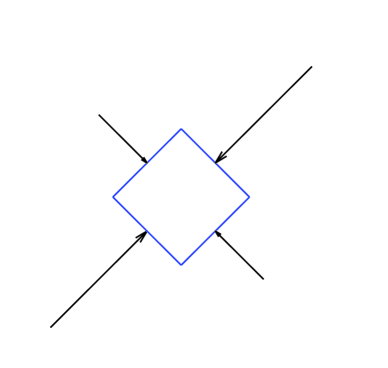
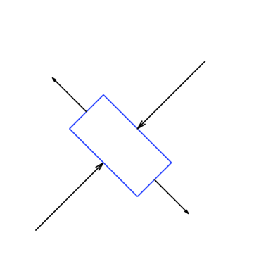
Refer to caption Refer to caption (a)π‘Ž\displaystyle(a) (b)𝑏\displaystyle(b) Minor stress axis Major stress axis Expansive strain-rate Contractive strain-rate

Figure 1: (a)π‘Ž\displaystyle(a) Illustrative stress eigenvectors; along the major axis the stress eigenvalue is βˆ’(p+‖𝝉‖)𝑝norm𝝉\displaystyle-(p+\|\mbox{\boldmath$\displaystyle\tau$}\|) with the minus sign indicating compression. (b)𝑏\displaystyle(b) A possible material deformation that is consistent with the stress field in (a)π‘Ž\displaystyle(a).

For a Coulomb material, which is assumed to be incompressible, the first constitutive relation states that Ο•italic-Ο•\displaystyle\phi is a constant. This then reduces (1) to the

Flow rule:div 𝒖=0.Flow rule:div 𝒖0\mbox{\bf Flow rule:}\qquad\mbox{div }\mbox{\boldmath$\displaystyle u$}=0\,. (3)

For the next constitutive relation the stress tensor

Οƒi​j=βˆ’p​δi​j+Ο„i​j,subscriptπœŽπ‘–π‘—π‘subscript𝛿𝑖𝑗subscriptπœπ‘–π‘—\sigma_{ij}=-p\delta_{ij}+\tau_{ij}\,, (4)

is decomposed into a pressure term (where p=βˆ’Οƒi​i/2𝑝subscriptπœŽπ‘–π‘–2\displaystyle p=-\sigma_{ii}/2) plus a trace-free tensor 𝝉𝝉\displaystyle\tau, called the deviatoric stress. The second relation is then the

Yield condition:‖𝝉‖=μ​p,Yield condition:normπ‰πœ‡π‘\mbox{\bf Yield condition:}\qquad\|\mbox{\boldmath$\displaystyle\tau$}\|=\mu p\,, (5)

where ΞΌπœ‡\displaystyle\mu is a constant and for any tensor 𝑻𝑻\displaystyle T the norm is defined by

‖𝑻‖=Ti​j​Ti​j/2.norm𝑻subscript𝑇𝑖𝑗subscript𝑇𝑖𝑗2\|\mbox{\boldmath$\displaystyle T$}\|=\sqrt{T_{ij}T_{ij}/2}\,. (6)

This yield condition expresses the idea that a granular material cannot deform unless the shear stress is sufficient to overcome friction111Thus, (5) contains the implicit assumption that material is actually deforming. Otherwise (5) must be replaced by inequality, ‖𝝉‖≀μ​pnormπ‰πœ‡π‘\displaystyle\|\mbox{\boldmath$\displaystyle\tau$}\|\leq\mu p, and the governing equations are underdetermined unless further relations, such as those of elasticity, are included.. The third constitutive relation requires that the eigenvectors of the deviatoric stress tensor and the deviatoric strain-rate tensor222Note that for incompressible flow, the full strain-rate tensor (βˆ‚jui+βˆ‚iuj)/2subscript𝑗subscript𝑒𝑖subscript𝑖subscript𝑒𝑗2\displaystyle(\partial_{j}u_{i}+\partial_{i}u_{j})/2 and the deviatoric strain-rate tensor are equal since the second term on the right in (7) vanishes.

Di​j=12​(βˆ‚jui+βˆ‚iuj)βˆ’12​(div 𝒖)​δi​j,subscript𝐷𝑖𝑗12subscript𝑗subscript𝑒𝑖subscript𝑖subscript𝑒𝑗12div 𝒖subscript𝛿𝑖𝑗D_{ij}=\frac{1}{2}(\partial_{j}u_{i}+\partial_{i}u_{j})-\frac{1}{2}(\mbox{div }\mbox{\boldmath$\displaystyle u$})\delta_{ij}\,, (7)

are aligned (see Figure 1 for motivation), which may be written

Alignment:Di​j‖𝑫‖=Ο„i​j‖𝝉‖.Alignment:subscript𝐷𝑖𝑗norm𝑫subscriptπœπ‘–π‘—norm𝝉\mbox{\bf Alignment:}\qquad\frac{D_{ij}}{\|\mbox{\boldmath$\displaystyle D$}\|}=\frac{\tau_{ij}}{\|\mbox{\boldmath$\displaystyle\tau$}\|}\,. (8)

In words (8) may be interpreted as asserting that in the space of trace-free symmetric 2Γ—222\displaystyle 2\times 2 matrices, which is two-dimensional, 𝑫𝑫\displaystyle D and 𝝉𝝉\displaystyle\tau are parallel. Thus, this matrix equation entails only one scalar relation. For reference below we record that

𝑫=12​[βˆ‚1u1βˆ’βˆ‚2u2βˆ‚1u2+βˆ‚2u1βˆ‚1u2+βˆ‚2u1βˆ‚2u2βˆ’βˆ‚1u1].𝑫12delimited-[]subscript1subscript𝑒1subscript2subscript𝑒2subscript1subscript𝑒2subscript2subscript𝑒1subscript1subscript𝑒2subscript2subscript𝑒1subscript2subscript𝑒2subscript1subscript𝑒1\mbox{\boldmath$\displaystyle D$}=\frac{1}{2}\left[\begin{array}[]{cc}\partial_{1}u_{1}-\partial_{2}u_{2}&\partial_{1}u_{2}+\partial_{2}u_{1}\\ \partial_{1}u_{2}+\partial_{2}u_{1}&\partial_{2}u_{2}-\partial_{1}u_{1}\end{array}\right]\,. (9)

It is customary [2], [5] to process these equations by expressing the deviatoric stress 𝝉𝝉\displaystyle\tau in terms of p𝑝\displaystyle p and the strain rate as follows:

Ο„i​j=‖𝝉‖​τi​j‖𝝉‖=μ​p​Di​j‖𝑫‖,subscriptπœπ‘–π‘—norm𝝉subscriptπœπ‘–π‘—normπ‰πœ‡π‘subscript𝐷𝑖𝑗norm𝑫\tau_{ij}=\|\mbox{\boldmath$\displaystyle\tau$}\|\frac{\tau_{ij}}{\|\mbox{\boldmath$\displaystyle\tau$}\|}=\mu p\frac{D_{ij}}{\|\mbox{\boldmath$\displaystyle D$}\|}\,, (10)

where we have invoked (5) and (8). We may substitute (10) into (2) to obtain

Οβˆ—β€‹Ο•β€‹(βˆ‚t+ujβ€‹βˆ‚j)​ui=βˆ‚j[μ​p‖𝑫‖​Di​j]βˆ’βˆ‚ip+Οβˆ—β€‹Ο•β€‹gi,subscript𝜌italic-Ο•subscript𝑑subscript𝑒𝑗subscript𝑗subscript𝑒𝑖subscript𝑗delimited-[]πœ‡π‘norm𝑫subscript𝐷𝑖𝑗subscript𝑖𝑝subscript𝜌italic-Ο•subscript𝑔𝑖\rho_{*}\phi(\partial_{t}+u_{j}\partial_{j})u_{i}=\partial_{j}\left[\frac{\mu p}{\|\mbox{\boldmath$\displaystyle D$}\|}D_{ij}\right]-\partial_{i}p+\rho_{*}\phi g_{i}\,, (11)

and the resulting equation, together with (3), gives three equations for pressure p𝑝\displaystyle p and velocity 𝒖𝒖\displaystyle u. In form, at least, these equations resemble the incompressible Navier-Stokes equation. However, in two dimensions (as considered here) they are always ill-posed [2].

2.2 Incompressible μ​(I)πœ‡πΌ\displaystyle\mu(I)-rheology

Work described by the Groupement De Recherche Milieux DivisΓ©s [4] has significantly improved the Coulomb model by including some rate dependence (in the sense of plasticity [25]) in the yield condition while making no changes in the incompressible flow rule (3) and the alignment condition (8). Specifically, a wide range of experiments is captured by replacing the constant ΞΌπœ‡\displaystyle\mu in (5) by an increasing function μ​(I)πœ‡πΌ\displaystyle\mu(I) of the inertial number,

I=2​d​‖𝐃‖p/Οβˆ—,𝐼2𝑑norm𝐃𝑝subscript𝜌I=\frac{2d\|\mathbf{D}\|}{\sqrt{p/\rho_{*}}}\,, (12)

where d𝑑\displaystyle d is the particle diameter. The expression

μ​(I)=ΞΌ1+ΞΌ2βˆ’ΞΌ1I0/I+1,πœ‡πΌsubscriptπœ‡1subscriptπœ‡2subscriptπœ‡1subscript𝐼0𝐼1\mu(I)=\mu_{1}+\frac{\mu_{2}-\mu_{1}}{I_{0}/I+1}\,, (13)

where ΞΌ1subscriptπœ‡1\displaystyle\mu_{1}, ΞΌ2subscriptπœ‡2\displaystyle\mu_{2} and I0subscript𝐼0\displaystyle I_{0} are constants with ΞΌ2>ΞΌ1subscriptπœ‡2subscriptπœ‡1\displaystyle\mu_{2}>\mu_{1}, is a frequently used form [26]. Below we shall assume that

μ′​(I)>0andμ′′​(I)<0.formulae-sequencesuperscriptπœ‡β€²πΌ0andsuperscriptπœ‡β€²β€²πΌ0\mu^{\prime}(I)>0\qquad\mbox{and}\qquad\mu^{\prime\prime}(I)<0\,. (14)

The modified yield condition changes (11) to read

Οβˆ—β€‹Ο•β€‹(βˆ‚t+ujβ€‹βˆ‚j)​ui=βˆ‚j[μ​(I)​p‖𝑫‖​Di​j]βˆ’βˆ‚ip+Οβˆ—β€‹Ο•β€‹gi.subscript𝜌italic-Ο•subscript𝑑subscript𝑒𝑗subscript𝑗subscript𝑒𝑖subscript𝑗delimited-[]πœ‡πΌπ‘norm𝑫subscript𝐷𝑖𝑗subscript𝑖𝑝subscript𝜌italic-Ο•subscript𝑔𝑖\rho_{*}\phi(\partial_{t}+u_{j}\partial_{j})u_{i}=\partial_{j}\left[\frac{\mu(I)p}{\|\mbox{\boldmath$\displaystyle D$}\|}D_{ij}\right]-\partial_{i}p+\rho_{*}\phi g_{i}\,. (15)

The effect of this seemingly small perturbation is profound. Unlike for Coulomb material, equations (15) and (3) are well-posed for a significant range of inertial numbers, specifically when the deformation rate is neither too small nor too large relative to the pressure [9].

2.3 Compressibility and I𝐼\displaystyle I-dependent rheology

We refer to Critical State Soil Mechanics (cf. Appendix 1) for guidance in introducing compressibility into the rheology. Thus, we make no change in the alignment condition (8); we assume Ο•italic-Ο•\displaystyle\phi-dependence in the yield condition,

‖𝝉‖=Y​(p,Ο•,I);normπ‰π‘Œπ‘italic-ϕ𝐼\|\mbox{\boldmath{$\displaystyle\tau$}}\|=Y(p,\phi,I)\,; (16)

and we allow for volumetric changes by introducing a new function f​(p,Ο•,I)𝑓𝑝italic-ϕ𝐼\displaystyle f(p,\phi,I) and modifying the flow rule to

div 𝒖=2​f​(p,Ο•,I)​‖𝐃‖.div 𝒖2𝑓𝑝italic-ϕ𝐼norm𝐃\mbox{div }\mbox{\boldmath$\displaystyle u$}=2f(p,\phi,I)\,\|\mathbf{D}\|\,. (17)

To get well posed equations, we require that the yield condition and the flow-rule functions are related by the equation333If Yπ‘Œ\displaystyle Y and f𝑓\displaystyle f are independent of I𝐼\displaystyle I, then (18) leads to the CSSM flow rule (71) derived from normality.

βˆ‚Yβˆ‚pβˆ’I2​pβ€‹βˆ‚Yβˆ‚I=f+Iβ€‹βˆ‚fβˆ‚I,π‘Œπ‘πΌ2π‘π‘ŒπΌπ‘“πΌπ‘“πΌ\frac{\partial Y}{\partial p}-\frac{I}{2p}\frac{\partial Y}{\partial I}=f+I\frac{\partial f}{\partial I}\,, (18)

and that they satisfy the inequalities

(a)Β β€‹βˆ‚IY>0and(b)Β β€‹βˆ‚pfβˆ’I2​pβ€‹βˆ‚If<0.formulae-sequence(a)Β subscriptπΌπ‘Œ0and(b)Β subscript𝑝𝑓𝐼2𝑝subscript𝐼𝑓0\mbox{(a) }\partial_{I}Y>0\qquad\mbox{and}\qquad\mbox{(b) }\partial_{p}f-\frac{I}{2p}\partial_{I}f<0\,. (19)

We may now state our main result, the well posedness theorem for the system (1), (2), (8), (16), (17), which we call the CIDR equations. (Mnemonic: compressible I𝐼\displaystyle I-dependent rheology.) The term linearly well posed is defined in Appendix 2, and the result is proved in Sections 3 and 4.


Theorem Under hypotheses (18) and (19), the CIDR system is linearly well posed.


Remark: The I𝐼\displaystyle I-dependence in these equations need not relate to a friction coefficient μ​(I)πœ‡πΌ\displaystyle\mu(I). In Β§2.5 we connect the equations to μ​(I)πœ‡πΌ\displaystyle\mu(I)-rheology.

2.4 Derivation of evolution equations

To place the equations in a larger continuum-mechanics context, we show that the CIDR equations of motion can be rewritten as a system of three evolution equations for the velocity 𝒖𝒖\displaystyle u and the solids fraction Ο•italic-Ο•\displaystyle\phi. In form, these equations are analogous to the Navier-Stokes equations for a viscous, compressible fluid. We make no use of this form of the equations in our proof of well-posedness.

We want to eliminate stresses from the equations of motion. To this end, we propose to solve for the mean stress p𝑝\displaystyle p using the flow rule (17), which we rewrite as

f​(p,Ο•,I)=div 𝒖2​‖𝐃‖.𝑓𝑝italic-ϕ𝐼div 𝒖2norm𝐃f(p,\phi,I)=\frac{\mbox{div }\mbox{\boldmath$\displaystyle u$}}{2\|\mathbf{D}\|}\,. (20)

Note that f​(p,Ο•,I)𝑓𝑝italic-ϕ𝐼\displaystyle f(p,\phi,I) depends on p𝑝\displaystyle p both directly in its first argument and indirectly through I=2​d​‖𝑫‖/p/Οβˆ—πΌ2𝑑norm𝑫𝑝subscript𝜌\displaystyle I=2d\|\mbox{\boldmath$\displaystyle D$}\|/\sqrt{p/\rho_{*}} in its third argument. However,

βˆ‚βˆ‚p​[f​(p,Ο•,2​d​‖𝑫‖/p/Οβˆ—)]=βˆ‚pfβˆ’I2​pβ€‹βˆ‚If,𝑝delimited-[]𝑓𝑝italic-Ο•2𝑑norm𝑫𝑝subscript𝜌subscript𝑝𝑓𝐼2𝑝subscript𝐼𝑓\frac{\partial}{\partial p}[f(p,\phi,2d\|\mbox{\boldmath$\displaystyle D$}\|/\sqrt{p/\rho_{*}})]=\partial_{p}f-\frac{I}{2p}\partial_{I}f\,, (21)

which by assumption (19b) is nonzero. Thus, we may apply the Implicit Function Theorem to (20) to solve p=P​(βˆ‡π’–,Ο•).π‘π‘ƒβˆ‡π’–italic-Ο•\displaystyle p=P(\nabla\mbox{\boldmath$\displaystyle u$},\phi).444Note that P𝑃\displaystyle P in fact depends only on div 𝒖,‖𝑫‖div 𝒖norm𝑫\displaystyle\mbox{div }\mbox{\boldmath$\displaystyle u$},\|\mbox{\boldmath$\displaystyle D$}\| and Ο•.italic-Ο•\displaystyle\phi. Given this, we may define

T​(βˆ‡π’–,Ο•)=Y​(P​(βˆ‡π’–,Ο•),Ο•,I​(βˆ‡π’–,Ο•))whereI​(βˆ‡π’–,Ο•)=2​d​‖𝑫‖P​(βˆ‡π’–,Ο•)/Οβˆ—,formulae-sequenceπ‘‡βˆ‡π’–italic-Ο•π‘Œπ‘ƒβˆ‡π’–italic-Ο•italic-Ο•πΌβˆ‡π’–italic-Ο•whereπΌβˆ‡π’–italic-Ο•2𝑑normπ‘«π‘ƒβˆ‡π’–italic-Ο•subscript𝜌\displaystyle T(\nabla\mbox{\boldmath$\displaystyle u$},\phi)=Y(P(\nabla\mbox{\boldmath$\displaystyle u$},\phi),\phi,I(\nabla\mbox{\boldmath$\displaystyle u$},\phi))\qquad\mbox{where}\qquad I(\nabla\mbox{\boldmath$\displaystyle u$},\phi)=\frac{2d\|\mbox{\boldmath$\displaystyle D$}\|}{\sqrt{P(\nabla\mbox{\boldmath$\displaystyle u$},\phi)/\rho_{*}}}\,,

and substitute into conservation of momentum to obtain an equation

Οβˆ—β€‹Ο•β€‹(βˆ‚t+ujβ€‹βˆ‚j)​ui=βˆ‚j[T​(βˆ‡π’–,Ο•)‖𝑫‖​Di​j]βˆ’βˆ‚i[P​(βˆ‡π’–,Ο•)]+Οβˆ—β€‹Ο•β€‹gi.subscript𝜌italic-Ο•subscript𝑑subscript𝑒𝑗subscript𝑗subscript𝑒𝑖subscript𝑗delimited-[]π‘‡βˆ‡π’–italic-Ο•norm𝑫subscript𝐷𝑖𝑗subscript𝑖delimited-[]π‘ƒβˆ‡π’–italic-Ο•subscript𝜌italic-Ο•subscript𝑔𝑖\rho_{*}\phi(\partial_{t}+u_{j}\partial_{j})u_{i}=\partial_{j}\left[\frac{T(\nabla\mbox{\boldmath$\displaystyle u$},\phi)}{\|\mbox{\boldmath$\displaystyle D$}\|}D_{ij}\right]-\partial_{i}[P(\nabla\mbox{\boldmath$\displaystyle u$},\phi)]+\rho_{*}\phi g_{i}\,. (22)

This equation, along with (1), gives a system of three evolution equations for the velocity 𝒖𝒖\displaystyle u and the solids fraction Ο•italic-Ο•\displaystyle\phi.

2.5 Connection to μ​(I)πœ‡πΌ\displaystyle\mu(I)-rheology

Without making any attempt to be general, we illustrate one example of how μ​(I)πœ‡πΌ\displaystyle\mu(I)-rheology may be included in constitutive relations of the form (16), (17). Motivated by equation (72) in Appendix 1, we make the ansatz

(a)Y​(p,Ο•,I)=α​(I)​pβˆ’p2/C​(Ο•)(b)f​(p,Ο•,I)=β​(I)βˆ’2​p/C​(Ο•).(a)π‘Œπ‘italic-ϕ𝐼𝛼𝐼𝑝superscript𝑝2𝐢italic-Ο•missing-subexpressionmissing-subexpressionmissing-subexpressionmissing-subexpression(b)𝑓𝑝italic-ϕ𝐼𝛽𝐼2𝑝𝐢italic-Ο•\begin{array}[]{cccl}\mbox{(a)}&Y(p,\phi,I)&=&\alpha(I)p-p^{2}/C(\phi)\\ \\ \mbox{(b)}&f(p,\phi,I)&=&\beta(I)-2p/C(\phi)\,.\end{array} (23)

In these equations, it is worth emphasising that p,Ο•,I𝑝italic-ϕ𝐼\displaystyle p,\phi,I are treated as independent variables, not to be confused with the dependence of I𝐼\displaystyle I on p𝑝\displaystyle p in the previous subsection. The function C​(Ο•)𝐢italic-Ο•\displaystyle C(\phi) is an increasing function of Ο•italic-Ο•\displaystyle\phi. As Ο•italic-Ο•\displaystyle\phi varies (with I𝐼\displaystyle I fixed) the yield loci ‖𝝉‖=Y​(p,Ο•,I)normπ‰π‘Œπ‘italic-ϕ𝐼\displaystyle\|\mbox{\boldmath{$\displaystyle\tau$}}\|=Y(p,\phi,I) derived from (23a) form a nested family of convex curves in stress space (cf. FigureΒ 2(b)). Observe from (17) that deformation without volumetric strain is possible if f​(p,Ο•,I)=0𝑓𝑝italic-ϕ𝐼0\displaystyle f(p,\phi,I)=0; i.e., for (23b), if p/C​(Ο•)=β​(I)/2𝑝𝐢italic-ϕ𝛽𝐼2\displaystyle p/C(\phi)=\beta(I)/2. Substituting this formula into (16) and using (23a), we derive

‖𝝉‖=[α​(I)βˆ’Ξ²β€‹(I)/2]​pnorm𝝉delimited-[]𝛼𝐼𝛽𝐼2𝑝\displaystyle\|\mbox{\boldmath{$\displaystyle\tau$}}\|=[\alpha(I)-\beta(I)/2]\;p

for such isochoric deformation to be possible. Thus, to recover the yield condition ‖𝝉‖=μ​(I)​pnormπ‰πœ‡πΌπ‘\displaystyle\|\mbox{\boldmath{$\displaystyle\tau$}}\|=\mu(I)p of the μ​(I)πœ‡πΌ\displaystyle\mu(I)-rheology, let us require that

α​(I)βˆ’Ξ²β€‹(I)/2=μ​(I).𝛼𝐼𝛽𝐼2πœ‡πΌ\alpha(I)-\beta(I)/2=\mu(I)\,. (24)

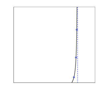
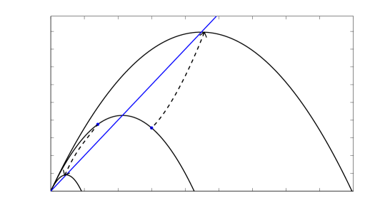
Refer to caption Refer to caption (a)π‘Ž\displaystyle(a) (b)𝑏\displaystyle(b) C𝐢\displaystyle C Ο•italic-Ο•\displaystyle\phi Ο•0subscriptitalic-Ο•0\displaystyle\phi_{0} Ο•0+Ξ΅subscriptitalic-Ο•0πœ€\displaystyle\phi_{0}+{\varepsilon} Ο•1subscriptitalic-Ο•1\displaystyle\phi_{1} Ο•2subscriptitalic-Ο•2\displaystyle\phi_{2} Ο•3subscriptitalic-Ο•3\displaystyle\phi_{3} Yπ‘Œ\displaystyle Y p𝑝\displaystyle p B𝐡\displaystyle B A𝐴\displaystyle A Ο•1subscriptitalic-Ο•1\displaystyle\phi_{1} Ο•2subscriptitalic-Ο•2\displaystyle\phi_{2} Ο•3subscriptitalic-Ο•3\displaystyle\phi_{3}

Figure 2: (a)π‘Ž\displaystyle(a) An example curve for the function C​(Ο•)𝐢italic-Ο•\displaystyle C(\phi) with a minimum solids volume fraction Ο•0subscriptitalic-Ο•0\displaystyle\phi_{0} and a vertical asymptote at Ο•0+O​(Ξ΅)subscriptitalic-Ο•0π‘‚πœ€\displaystyle\phi_{0}+O({\varepsilon}). (b)𝑏\displaystyle(b) Nested yield surfaces of the form (23) for a fixed value of I𝐼\displaystyle I with differing solids volume fractions. (The solid blue line, the dashed arrows, and the labels A𝐴\displaystyle A and B𝐡\displaystyle B refer to a discussion of CSSM in the AppendixΒ 1.)

Lemma 1. Equations (18) and (24) imply that

α​(I)=45​μ​(I)+1225​Iβˆ’2/5β€‹βˆ«0II~βˆ’3/5​μ​(I~)​𝑑I~𝛼𝐼45πœ‡πΌ1225superscript𝐼25superscriptsubscript0𝐼superscript~𝐼35πœ‡~𝐼differential-d~𝐼\alpha(I)=\frac{4}{5}\mu(I)+\frac{12}{25}I^{-2/5}\int_{0}^{I}\tilde{I}^{-3/5}\mu(\tilde{I})d\tilde{I} (25)

and

β​(I)=βˆ’25​μ​(I)+2425​Iβˆ’2/5β€‹βˆ«0II~βˆ’3/5​μ​(I~)​𝑑I~.𝛽𝐼25πœ‡πΌ2425superscript𝐼25superscriptsubscript0𝐼superscript~𝐼35πœ‡~𝐼differential-d~𝐼\beta(I)=-\frac{2}{5}\mu(I)+\frac{24}{25}I^{-2/5}\int_{0}^{I}\tilde{I}^{-3/5}\mu(\tilde{I})d\tilde{I}\,. (26)

.


Proof: Β Substituting the relations (23) into (18), and using (24) to eliminate Ξ²,𝛽\displaystyle\beta, we derive the linear ordinary differential equation for Ξ±=α​(I)::𝛼𝛼𝐼absent\displaystyle\alpha=\alpha(I):

52​I​α′​(I)+α​(I)=2​μ​(I)+2​I​μ′​(I).52𝐼superscript𝛼′𝐼𝛼𝐼2πœ‡πΌ2𝐼superscriptπœ‡β€²πΌ\frac{5}{2}I\alpha^{\prime}(I)+\alpha(I)=2\mu(I)+2I\mu^{\prime}(I)\,. (27)

Solving this linear equation for α​(I),𝛼𝐼\displaystyle\alpha(I), with an integrating factor, we obtain

I2/5​α​(I)=45β€‹βˆ«0II~βˆ’3/5​μ​(I~)​𝑑I~+45β€‹βˆ«0II~2/5​μ′​(I~)​𝑑I~,superscript𝐼25𝛼𝐼45superscriptsubscript0𝐼superscript~𝐼35πœ‡~𝐼differential-d~𝐼45superscriptsubscript0𝐼superscript~𝐼25superscriptπœ‡β€²~𝐼differential-d~𝐼\displaystyle I^{2/5}\alpha(I)=\frac{4}{5}\int_{0}^{I}\tilde{I}^{-3/5}\mu(\tilde{I})d\tilde{I}+\frac{4}{5}\int_{0}^{I}\tilde{I}^{2/5}\mu^{\prime}(\tilde{I})d\tilde{I}\,,

from which the formula (25) follows after integrating the second integral by parts. Finally, substituting this formula for α​(I)𝛼𝐼\displaystyle\alpha(I) into (24), we obtain the formula (26) for β​(I).𝛽𝐼\displaystyle\beta(I). Β 


Lemma 2. The yield condition and flow-rule function (23a,b) that follow from (25), (26) verify hypotheses (18) and (19), provided μ​(I)πœ‡πΌ\displaystyle\mu(I) satisfies (14).


Proof: Β Of course (18) is satisfied because this equation was imposed in deriving (25), (26).

Differentiating (23b), we see that βˆ‚pf​(p,Ο•,I)=βˆ’2/C​(Ο•)<0.subscript𝑝𝑓𝑝italic-ϕ𝐼2𝐢italic-Ο•0\displaystyle\partial_{p}f(p,\phi,I)=-2/C(\phi)<0. To calculate βˆ‚If​(p,Ο•,I),subscript𝐼𝑓𝑝italic-ϕ𝐼\displaystyle\partial_{I}f(p,\phi,I), we first reparametrize the integral in (26) to obtain β​(I)=βˆ’25​μ​(I)+2425β€‹βˆ«01sβˆ’3/5​μ​(s​I)​𝑑s.𝛽𝐼25πœ‡πΌ2425superscriptsubscript01superscript𝑠35πœ‡π‘ πΌdifferential-d𝑠\displaystyle\beta(I)=-\frac{2}{5}\mu(I)+\frac{24}{25}\int_{0}^{1}s^{-3/5}\mu(sI)ds\,. Then

βˆ‚If​(p,Ο•,I)=β′​(I)=βˆ’25​μ′​(I)+2425β€‹βˆ«01s2/5​μ′​(s​I)​𝑑s.subscript𝐼𝑓𝑝italic-ϕ𝐼superscript𝛽′𝐼25superscriptπœ‡β€²πΌ2425superscriptsubscript01superscript𝑠25superscriptπœ‡β€²π‘ πΌdifferential-d𝑠\displaystyle\partial_{I}f(p,\phi,I)=\beta^{\prime}(I)=-\frac{2}{5}\mu^{\prime}(I)+\frac{24}{25}\int_{0}^{1}s^{2/5}\mu^{\prime}(sI)ds\,.

By (14), μ′′​(I)<0superscriptπœ‡β€²β€²πΌ0\displaystyle\,\mu^{\prime\prime}(I)<0, so μ′​(s​I)>μ′​(I)superscriptπœ‡β€²π‘ πΌsuperscriptπœ‡β€²πΌ\displaystyle\mu^{\prime}(sI)>\mu^{\prime}(I) for 0<s<1.0𝑠1\displaystyle 0<s<1. Thus,

β′​(I)>μ′​(I)​{βˆ’25+2425β€‹βˆ«01s2/5​𝑑s}=μ′​(I)​{2435βˆ’25}>0,superscript𝛽′𝐼superscriptπœ‡β€²πΌ252425superscriptsubscript01superscript𝑠25differential-d𝑠superscriptπœ‡β€²πΌ2435250\displaystyle\beta^{\prime}(I)>\mu^{\prime}(I)\left\{-\frac{2}{5}+\frac{24}{25}\int_{0}^{1}s^{2/5}ds\right\}=\mu^{\prime}(I)\left\{\frac{24}{35}-\frac{2}{5}\right\}>0\,,

the last inequality using (14). Consequently,

βˆ‚pf​(p,Ο•,I)βˆ’I2​pβ€‹βˆ‚If​(p,Ο•,I)<0,subscript𝑝𝑓𝑝italic-ϕ𝐼𝐼2𝑝subscript𝐼𝑓𝑝italic-ϕ𝐼0\partial_{p}f(p,\phi,I)-\frac{I}{2p}\partial_{I}f(p,\phi,I)<0\,, (28)

proving inequality (19b).

For inequality (19a), we reparametrize the integral (25) and differentiate to obtain

βˆ‚IY​(p,Ο•,I)=α′​(I)​p=p​(45​μ′​(I)+1225β€‹βˆ«01s2/5​μ′​(s​I)​𝑑s)>0,subscriptπΌπ‘Œπ‘italic-ϕ𝐼superscript𝛼′𝐼𝑝𝑝45superscriptπœ‡β€²πΌ1225superscriptsubscript01superscript𝑠25superscriptπœ‡β€²π‘ πΌdifferential-d𝑠0\displaystyle\partial_{I}Y(p,\phi,I)=\alpha^{\prime}(I)p=p\left(\frac{4}{5}\mu^{\prime}(I)+\frac{12}{25}\int_{0}^{1}s^{2/5}\mu^{\prime}(sI)ds\right)>0\,,

as desired. Β 


Based on an analogy with CSSM, let us suppose that C​(Ο•)𝐢italic-Ο•\displaystyle C(\phi) is a sensitive function of Ο•italic-Ο•\displaystyle\phi, say of the form

C​(Ο•)=C~​(Ο•βˆ’Ο•0Ξ΅)𝐢italic-Ο•~𝐢italic-Ο•subscriptitalic-Ο•0πœ€C(\phi)=\tilde{C}\left(\frac{\phi-\phi_{0}}{{\varepsilon}}\right) (29)

where Ο•0subscriptitalic-Ο•0\displaystyle\phi_{0} is the minimum solids fraction for sustained stress transmission between grains (random loose packing), Ξ΅πœ€\displaystyle{\varepsilon} is a small parameter, and for definiteness we may take C~​(z)=z/(1βˆ’z)~𝐢𝑧𝑧1𝑧\displaystyle\tilde{C}(z)=z/(1-z) as in figure 2. Note that C​(Ο•)𝐢italic-Ο•\displaystyle C(\phi) diverges as Ο•β†’Ο•0+Ξ΅β†’italic-Ο•subscriptitalic-Ο•0πœ€\displaystyle\phi\to\phi_{0}+{\varepsilon}; thus, (29) requires that Ο•italic-Ο•\displaystyle\phi is confined to a narrow range,

Ο•0≀ϕ<Ο•0+Ξ΅.subscriptitalic-Ο•0italic-Ο•subscriptitalic-Ο•0πœ€\phi_{0}\leq\phi<\phi_{0}+{\varepsilon}\,. (30)

In physical terms, the maximum solids fraction Ο•0+Ξ΅subscriptitalic-Ο•0πœ€\displaystyle\phi_{0}+{\varepsilon} represents the jamming threshold. We call the limit Ξ΅β†’0β†’πœ€0\displaystyle{\varepsilon}\to 0 incompressible because, as may be seen from (30), the density of material becomes essentially constant.


Lemma 3. As Ξ΅β†’0β†’πœ€0\displaystyle{\varepsilon}\to 0, the CIDR equations reduce to the equations of incompressible μ​(I)πœ‡πΌ\displaystyle\mu(I)-rheology, (3), (15).


Proof: Β We process the CIDR equations, which have the six unknowns Ο•italic-Ο•\displaystyle\phi, uisubscript𝑒𝑖\displaystyle u_{i}, and Οƒi​jsubscriptπœŽπ‘–π‘—\displaystyle\sigma_{ij}, as follows. First we reduce to five unknownsβ€”Ο•italic-Ο•\displaystyle\phi, uisubscript𝑒𝑖\displaystyle u_{i}, p𝑝\displaystyle p and Ο„=β€–π‰β€–πœnorm𝝉\displaystyle\tau=\|\mbox{\boldmath{$\displaystyle\tau$}}\|β€”by recalling the definition (4) and the alignment condition (8) to write

Οƒi​j=βˆ’p​δi​j+τ​Di​j‖𝑫‖.subscriptπœŽπ‘–π‘—π‘subscriptπ›Ώπ‘–π‘—πœsubscript𝐷𝑖𝑗norm𝑫\displaystyle\sigma_{ij}=-p\delta_{ij}+\tau\frac{D_{ij}}{\|\mbox{\boldmath$\displaystyle D$}\|}\,.

Next we use the yield condition to eliminate Ο•italic-Ο•\displaystyle\phi, reducing this number to four. Specifically, substituting (23a) into (16), we write the yield condition

Ο„=α​(I)​pβˆ’p2/C​(Ο•).πœπ›ΌπΌπ‘superscript𝑝2𝐢italic-Ο•\tau=\alpha(I)p-p^{2}/C(\phi)\,. (31)

Solving (31) for Ο•italic-Ο•\displaystyle\phi we obtain

Ο•=Φ​(βˆ‡π’–,p,Ο„)=Cβˆ’1​(p2α​(I)​pβˆ’Ο„),italic-Ο•Ξ¦βˆ‡π’–π‘πœsuperscript𝐢1superscript𝑝2π›ΌπΌπ‘πœ\phi=\Phi(\nabla\mbox{\boldmath$\displaystyle u$},p,\tau)=C^{-1}\left(\frac{p^{2}}{\alpha(I)p-\tau}\right)\,, (32)

where the dependence on βˆ‡π’–βˆ‡π’–\displaystyle\nabla\mbox{\boldmath$\displaystyle u$} comes from the fact that I=2​d​‖𝑫‖/p/Οβˆ—.𝐼2𝑑norm𝑫𝑝subscript𝜌\displaystyle I=2d\|\mbox{\boldmath$\displaystyle D$}\|/\sqrt{p/\rho_{*}}. Substitution of this formula into the conservation laws (1), (2) yields the equations

(βˆ‚t+ujβ€‹βˆ‚j)​Φ​(βˆ‡π’–,p,Ο„)+Φ​(βˆ‡π’–,p,Ο„)​div 𝒖subscript𝑑subscript𝑒𝑗subscriptπ‘—Ξ¦βˆ‡π’–π‘πœΞ¦βˆ‡π’–π‘πœdiv 𝒖\displaystyle\displaystyle(\partial_{t}+u_{j}\partial_{j})\Phi(\nabla\mbox{\boldmath$\displaystyle u$},p,\tau)+\Phi(\nabla\mbox{\boldmath$\displaystyle u$},p,\tau)\,\mbox{div }\mbox{\boldmath$\displaystyle u$} =0,absent0\displaystyle\displaystyle=0\,, (33a)
Οβˆ—β€‹Ξ¦β€‹(βˆ‡π’–,p,Ο„)​(βˆ‚t+ujβ€‹βˆ‚j)​uisubscriptπœŒΞ¦βˆ‡π’–π‘πœsubscript𝑑subscript𝑒𝑗subscript𝑗subscript𝑒𝑖\displaystyle\displaystyle\rho_{*}\Phi(\nabla\mbox{\boldmath$\displaystyle u$},p,\tau)(\partial_{t}+u_{j}\partial_{j})u_{i} =βˆ‚j[τ‖𝑫‖​Di​j]βˆ’βˆ‚ip+Οβˆ—β€‹Ξ¦β€‹gi.absentsubscript𝑗delimited-[]𝜏norm𝑫subscript𝐷𝑖𝑗subscript𝑖𝑝subscript𝜌Φsubscript𝑔𝑖\displaystyle\displaystyle=\partial_{j}\left[\frac{\tau}{\|\mbox{\boldmath$\displaystyle D$}\|}D_{ij}\right]-\partial_{i}p+\rho_{*}\Phi g_{i}\,. (33b)

Finally, we show the flow rule (17) may be rewritten

div 𝒖=4​[Ο„/pβˆ’ΞΌβ€‹(I)]​‖𝐃‖.div 𝒖4delimited-[]πœπ‘πœ‡πΌnorm𝐃\mbox{div }\mbox{\boldmath$\displaystyle u$}=4[\tau/p-\mu(I)]\,\|\mathbf{D}\|\,. (34)

To see this, we combine (23b) with (24) to conclude

f​(p,Ο•,I)=β​(I)βˆ’2​p/C​(Ο•)=2​[α​(I)βˆ’ΞΌβ€‹(I)]βˆ’2​p/C​(Ο•)𝑓𝑝italic-ϕ𝐼𝛽𝐼2𝑝𝐢italic-Ο•2delimited-[]π›ΌπΌπœ‡πΌ2𝑝𝐢italic-Ο•\displaystyle f(p,\phi,I)=\beta(I)-2p/C(\phi)=2[\alpha(I)-\mu(I)]-2p/C(\phi)

and substitute the relation α​(I)=Ο„/p+p/C​(Ο•)π›ΌπΌπœπ‘π‘πΆitalic-Ο•\displaystyle\alpha(I)=\tau/p+p/C(\phi) derived by manipulating (31). Thus, the system (33), (34) governs the evolution of the four unknowns uisubscript𝑒𝑖\displaystyle u_{i}, p𝑝\displaystyle p, and Ο„πœ\displaystyle\tau.

Now we claim that if C​(Ο•)𝐢italic-Ο•\displaystyle C(\phi) has the form (29), then (33), (34) is a singular perturbation of (3), (15). It follows from (29) that (32) has the expansion

Ο•=Ο•0+Ρ​Φ~​(βˆ‡π’–,p,Ο„),italic-Ο•subscriptitalic-Ο•0πœ€~Ξ¦βˆ‡π’–π‘πœ\phi=\phi_{0}+{\varepsilon}\tilde{\Phi}(\nabla\mbox{\boldmath$\displaystyle u$},p,\tau)\,, (35)

where Ξ¦~​(βˆ‡π’–,p,Ο„)=C~βˆ’1​(p2/[α​(I)​pβˆ’Ο„])~Ξ¦βˆ‡π’–π‘πœsuperscript~𝐢1superscript𝑝2delimited-[]π›ΌπΌπ‘πœ\displaystyle\tilde{\Phi}(\nabla\mbox{\boldmath$\displaystyle u$},p,\tau)=\tilde{C}^{-1}(p^{2}/[\alpha(I)p-\tau]). Substituting (35) into the continuity equation (33a) we find

Ρ​(βˆ‚t+ujβ€‹βˆ‚j)​Φ~​(βˆ‡π’–,p,Ο„)+[Ο•0+Ρ​Φ~​(βˆ‡π’–,p,Ο„)]​div 𝒖=0.πœ€subscript𝑑subscript𝑒𝑗subscript𝑗~Ξ¦βˆ‡π’–π‘πœdelimited-[]subscriptitalic-Ο•0πœ€~Ξ¦βˆ‡π’–π‘πœdiv 𝒖0\displaystyle{\varepsilon}(\partial_{t}+u_{j}\partial_{j})\tilde{\Phi}(\nabla\mbox{\boldmath$\displaystyle u$},p,\tau)+[\phi_{0}+{\varepsilon}\tilde{\Phi}(\nabla\mbox{\boldmath$\displaystyle u$},p,\tau)]\,\mbox{div }\mbox{\boldmath$\displaystyle u$}=0\,.

If Ξ΅=0πœ€0\displaystyle{\varepsilon}=0 then this equation reduces to div 𝒖=0div 𝒖0\displaystyle\mbox{div }\mbox{\boldmath$\displaystyle u$}=0, although this is of course a highly singular limit. Thus, if Ξ΅=0πœ€0\displaystyle{\varepsilon}=0, the left hand side of (34) vanishes, so this equation simplifies to the yield condition Ο„=μ​(I)​pπœπœ‡πΌπ‘\displaystyle\tau=\mu(I)p, and substitution into (33b) yields (15). This proves the lemma. Β 

3 Proofs, Part I: Linearization

3.1 An alternative formulation of the alignment condition

It is convenient to study the linearized equations with a reformulated alignment condition that describes stress in terms of eigenvectors of, rather than entries of, the stress tensor. Since 𝝉𝝉\displaystyle\tau defined by (4) has trace zero, it has eigenvalues555Hence 𝝈𝝈\displaystyle\sigma has eigenvalues βˆ’p±‖𝝉‖plus-or-minus𝑝norm𝝉\displaystyle-p\pm\|\mbox{\boldmath{$\displaystyle\tau$}}\|. Note that βˆ’pβˆ’β€–π‰β€–π‘norm𝝉\displaystyle-p-\|\mbox{\boldmath{$\displaystyle\tau$}}\| is the major stress eigenvalueβ€”although this eigenvalue is the smaller algebraically, it is the larger in absolute value. ±‖𝝉‖plus-or-minusnorm𝝉\displaystyle\pm\|\mbox{\boldmath{$\displaystyle\tau$}}\|. Taking Οˆπœ“\displaystyle\psi as the angle that the eigenvector with eigenvalue βˆ’β€–π‰β€–norm𝝉\displaystyle-\|\mbox{\boldmath{$\displaystyle\tau$}}\| makes with the x1subscriptπ‘₯1\displaystyle x_{1}-axis gives

𝝉=βˆ’β€–π‰β€–β€‹[cos⁑2β€‹Οˆsin⁑2β€‹Οˆsin⁑2β€‹Οˆβˆ’cos⁑2β€‹Οˆ],𝝉norm𝝉delimited-[]2πœ“2πœ“2πœ“2πœ“\mbox{\boldmath$\displaystyle\tau$}=-\|\mbox{\boldmath$\displaystyle\tau$}\|\left[\begin{array}[]{cc}\cos 2\psi&\sin 2\psi\\ \sin 2\psi&-\cos 2\psi\end{array}\right]\,, (36)

which may be verified by checking that (cos⁑ψ,sin⁑ψ)πœ“πœ“\displaystyle(\cos\psi,\sin\psi) is an eigenvector of this matrix with eigenvalue βˆ’β€–π‰β€–norm𝝉\displaystyle-\|\mbox{\boldmath{$\displaystyle\tau$}}\|. Thus, the stress tensor Οƒi​jsubscriptπœŽπ‘–π‘—\displaystyle\sigma_{ij} is completely specified by the three scalars p𝑝\displaystyle p, ‖𝝉‖norm𝝉\displaystyle\|\mbox{\boldmath$\displaystyle\tau$}\|, and Οˆπœ“\displaystyle\psi.

Focusing on the first rows of the strain-rate tensor (9) and of (36), we extract from the matrix equation (8) the vector equation

(βˆ‚1u1βˆ’βˆ‚2u2,βˆ‚1u2+βˆ‚2u1)=k​(cos⁑2β€‹Οˆ,sin⁑2β€‹Οˆ),subscript1subscript𝑒1subscript2subscript𝑒2subscript1subscript𝑒2subscript2subscript𝑒1π‘˜2πœ“2πœ“(\partial_{1}u_{1}-\partial_{2}u_{2},\partial_{1}u_{2}+\partial_{2}u_{1})=k(\cos 2\psi,\sin 2\psi)\,, (37)

where k=βˆ’2​‖𝑫‖<0π‘˜2norm𝑫0\displaystyle k=-2\|\mbox{\boldmath$\displaystyle D$}\|<0. Since 𝑫𝑫\displaystyle D and 𝝉𝝉\displaystyle\tau lie in the two-dimensional space of trace-free, symmetric matrices, (37) is equivalent to (8). It follows from (37) that

Alt. alignment:(βˆ‚1u2+βˆ‚2u1)​cos⁑2β€‹Οˆβˆ’(βˆ‚1u1βˆ’βˆ‚2u2)​sin⁑2β€‹Οˆ=0.Alt. alignment:subscript1subscript𝑒2subscript2subscript𝑒12πœ“subscript1subscript𝑒1subscript2subscript𝑒22πœ“0\mbox{\bf Alt. alignment:}\qquad(\partial_{1}u_{2}+\partial_{2}u_{1})\cos 2\psi-(\partial_{1}u_{1}-\partial_{2}u_{2})\sin 2\psi=0\,. (38)

In point of fact, this equation is slightly weaker than the alignment condition since (38) is consistent with the possibility that k>0π‘˜0\displaystyle k>0 in (37); to rule out the latter possibility we impose the supplemental inequality666It is also true that (βˆ‚1u2+βˆ‚2u1)​sin⁑2β€‹Οˆβ‰€0subscript1subscript𝑒2subscript2subscript𝑒12πœ“0\displaystyle(\partial_{1}u_{2}+\partial_{2}u_{1})\sin 2\psi\leq 0, and if cos⁑2β€‹Οˆ2πœ“\displaystyle\cos 2\psi were to vanish, we would need to use this inequality to guarantee that k<0π‘˜0\displaystyle k<0. However, this issue will not arise in the analysis below. that

(βˆ‚1u1βˆ’βˆ‚2u2)​cos⁑2β€‹Οˆβ‰€0.subscript1subscript𝑒1subscript2subscript𝑒22πœ“0(\partial_{1}u_{1}-\partial_{2}u_{2})\cos 2\psi\leq 0\,. (39)

3.2 The calculation

Substitution of the stress tensor (36) into the momentum balance equations (2) allows for the full set of equations to be written as

Οβˆ—β€‹Ο•β€‹(βˆ‚t+u1β€‹βˆ‚1+u2β€‹βˆ‚2)​u1+βˆ‚1[p+τ​cos⁑(2β€‹Οˆ)]+βˆ‚2[τ​sin⁑(2β€‹Οˆ)]subscript𝜌italic-Ο•subscript𝑑subscript𝑒1subscript1subscript𝑒2subscript2subscript𝑒1subscript1delimited-[]π‘πœ2πœ“subscript2delimited-[]𝜏2πœ“\displaystyle\displaystyle\rho_{*}\phi\left(\partial_{t}+u_{1}\partial_{1}+u_{2}\partial_{2}\right)u_{1}+\partial_{1}\left[p+\tau\cos(2\psi)\right]+\partial_{2}\left[\tau\sin(2\psi)\right] =Οβˆ—β€‹Ο•β€‹g1,absentsubscript𝜌italic-Ο•subscript𝑔1\displaystyle\displaystyle=\rho_{*}\phi g_{1}\,, (40a)
Οβˆ—β€‹Ο•β€‹(βˆ‚t+u1β€‹βˆ‚1+u2β€‹βˆ‚2)​u2+βˆ‚1[τ​sin⁑(2β€‹Οˆ)]+βˆ‚2[pβˆ’Ο„β€‹cos⁑(2β€‹Οˆ)]subscript𝜌italic-Ο•subscript𝑑subscript𝑒1subscript1subscript𝑒2subscript2subscript𝑒2subscript1delimited-[]𝜏2πœ“subscript2delimited-[]π‘πœ2πœ“\displaystyle\displaystyle\rho_{*}\phi\left(\partial_{t}+u_{1}\partial_{1}+u_{2}\partial_{2}\right)u_{2}+\partial_{1}\left[\tau\sin(2\psi)\right]+\partial_{2}\left[p-\tau\cos(2\psi)\right] =Οβˆ—β€‹Ο•β€‹g2,absentsubscript𝜌italic-Ο•subscript𝑔2\displaystyle\displaystyle=\rho_{*}\phi g_{2}\,, (40b)
(βˆ‚t+u1β€‹βˆ‚1+u2β€‹βˆ‚2)​ϕ+ϕ​(βˆ‚1u1+βˆ‚2u2)subscript𝑑subscript𝑒1subscript1subscript𝑒2subscript2italic-Ο•italic-Ο•subscript1subscript𝑒1subscript2subscript𝑒2\displaystyle\displaystyle(\partial_{t}+u_{1}\partial_{1}+u_{2}\partial_{2})\phi+\phi\left(\partial_{1}u_{1}+\partial_{2}u_{2}\right) =0,absent0\displaystyle\displaystyle=0\,, (40c)
βˆ‚1u1+βˆ‚2u2subscript1subscript𝑒1subscript2subscript𝑒2\displaystyle\displaystyle\partial_{1}u_{1}+\partial_{2}u_{2} =2​f​‖𝑫‖,absent2𝑓norm𝑫\displaystyle\displaystyle=2f\|\mbox{\boldmath$\displaystyle D$}\|\,, (40d)
(βˆ‚2u1+βˆ‚1u2)​cos⁑(2β€‹Οˆ)+(βˆ‚2u2βˆ’βˆ‚1u1)​sin⁑(2β€‹Οˆ)subscript2subscript𝑒1subscript1subscript𝑒22πœ“subscript2subscript𝑒2subscript1subscript𝑒12πœ“\displaystyle\displaystyle\left(\partial_{2}u_{1}+\partial_{1}u_{2}\right)\cos(2\psi)+\left(\partial_{2}u_{2}-\partial_{1}u_{1}\right)\sin(2\psi) =0.absent0\displaystyle\displaystyle=0\,. (40e)

This system has five scalar unknowns, 𝑼=(u1,u2,Ο•,p,ψ)𝑼subscript𝑒1subscript𝑒2italic-Ο•π‘πœ“\displaystyle\mbox{\boldmath$\displaystyle U$}=(u_{1},u_{2},\phi,p,\psi). In (40a),(40b), Ο„πœ\displaystyle\,\tau is a mnemonically suggestive abbreviation for the yield function Y​(p,Ο•,I)π‘Œπ‘italic-ϕ𝐼\displaystyle Y(p,\phi,I) in (16), and in (40d), a repetition of (17), the function f𝑓\displaystyle f depends on arguments (p,Ο•,I)𝑝italic-ϕ𝐼\displaystyle(p,\phi,I) that are not written explicitly.

As in AppendixΒ 2, to linearise the equations we substitute a perturbation of a base solution 𝑼(0)​(𝐱,t)superscript𝑼0𝐱𝑑\displaystyle\mbox{\boldmath$\displaystyle U$}^{(0)}({\mathbf{x}},t), say

𝑼=𝑼(0)+𝑼^,𝑼superscript𝑼0bold-^𝑼\mbox{\boldmath$\displaystyle U$}=\mbox{\boldmath$\displaystyle U$}^{(0)}+\mbox{\boldmath$\displaystyle\hat{U}$}\,, (41)

into the equations, retain only terms that are linear in the perturbation 𝑼^bold-^𝑼\displaystyle\hat{U}, and freeze the coefficients at an arbitrary point (π±βˆ—,tβˆ—)superscript𝐱superscript𝑑\displaystyle({\mathbf{x}}^{*},t^{*}). It is convenient to temporarily drop most terms not of maximal order and estimate their effect in a calculation at the end of the argument. For example, this construction applied to (40c) yields the the constant-coefficient, linear equation

(βˆ‚t+u1βˆ—β€‹βˆ‚1+u2βˆ—β€‹βˆ‚2)​ϕ^+Ο•βˆ—β€‹(βˆ‚1u^1+βˆ‚2u^2)=0subscript𝑑superscriptsubscript𝑒1subscript1superscriptsubscript𝑒2subscript2^italic-Ο•superscriptitalic-Ο•subscript1subscript^𝑒1subscript2subscript^𝑒20(\partial_{t}+u_{1}^{*}\,\partial_{1}+u_{2}^{*}\,\partial_{2})\hat{\phi}+\phi^{*}(\partial_{1}\hat{u}_{1}+\partial_{2}\hat{u}_{2})=0 (42)

where ujβˆ—=uj(0)​(π±βˆ—,tβˆ—)superscriptsubscript𝑒𝑗subscriptsuperscript𝑒0𝑗superscript𝐱superscript𝑑\displaystyle u_{j}^{*}=u^{(0)}_{j}({\mathbf{x}}^{*},t^{*}) and Ο•βˆ—=Ο•(0)​(π±βˆ—,tβˆ—)superscriptitalic-Ο•superscriptitalic-Ο•0superscript𝐱superscript𝑑\displaystyle\phi^{*}=\phi^{(0)}({\mathbf{x}}^{*},t^{*}). Lower-order terms βˆ‚jΟ•βˆ—β€‹uj^subscript𝑗superscriptitalic-Ο•^subscript𝑒𝑗\displaystyle\partial_{j}\phi^{*}\,\hat{u_{j}} and βˆ‚jujβˆ—β€‹Ο•^subscript𝑗superscriptsubscript𝑒𝑗^italic-Ο•\displaystyle\partial_{j}u_{j}^{*}\,\hat{\phi} in the full linearisation of (40c) have been dropped in (42).
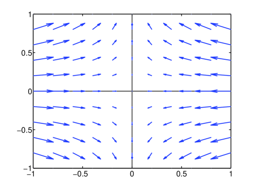
Refer to caption x2subscriptπ‘₯2\displaystyle x_{2} x1subscriptπ‘₯1\displaystyle x_{1}

Figure 3: An example of a base-state velocity field for the strain-rate tensor (43) with βˆ‚1u1(0)β‰‘βˆ’1subscript1superscriptsubscript𝑒101\displaystyle\partial_{1}u_{1}^{(0)}\equiv-1 and βˆ‚2u2(0)≑1/2subscript2superscriptsubscript𝑒2012\displaystyle\partial_{2}u_{2}^{(0)}\equiv 1/2.

In expanding the fully nonlinear factor ‖𝑫‖norm𝑫\displaystyle\|\mbox{\boldmath$\displaystyle D$}\| in (40d), we may take advantage of the rotational invariance of the equations to arrange that Οˆβˆ—=0superscriptπœ“0\displaystyle\psi^{*}=0; i.e., we may calculate in a rotated coordinate system for which, at (π±βˆ—,tβˆ—)superscript𝐱superscript𝑑\displaystyle({\mathbf{x}}^{*},t^{*}), the x1subscriptπ‘₯1\displaystyle x_{1}-axis is the maximal stress axis. Then by the alignment condition (38) the base-state deviatoric strain-rate tensor is diagonal at (π±βˆ—,tβˆ—)superscript𝐱superscript𝑑\displaystyle({\mathbf{x}}^{*},t^{*})

π‘«βˆ—=[(βˆ‚1u1βˆ—βˆ’βˆ‚2u2βˆ—)/200(βˆ‚2u2βˆ—βˆ’βˆ‚1u1βˆ—)/2],superscript𝑫delimited-[]subscript1superscriptsubscript𝑒1subscript2superscriptsubscript𝑒2200subscript2superscriptsubscript𝑒2subscript1superscriptsubscript𝑒12\mbox{\boldmath$\displaystyle D$}^{*}=\left[\begin{array}[]{cc}\left(\partial_{1}u_{1}^{*}-\partial_{2}u_{2}^{*}\right)/2&0\\ 0&\left(\partial_{2}u_{2}^{*}-\partial_{1}u_{1}^{*}\right)/2\end{array}\right]\,, (43)

and by (39), in the 1,1-position of this matrix βˆ‚1u1βˆ—βˆ’βˆ‚2u2βˆ—<0subscript1superscriptsubscript𝑒1subscript2superscriptsubscript𝑒20\displaystyle\partial_{1}u_{1}^{*}-\partial_{2}u_{2}^{*}<0. This corresponds to non-zero compression along the major stress axis, as illustrated in Figure 3. Now

β€–(π‘«βˆ—+𝑫^)β€–normsuperscript𝑫bold-^𝑫\displaystyle\displaystyle\|(\mbox{\boldmath$\displaystyle D$}^{*}+\mbox{\boldmath$\displaystyle\hat{D}$})\| =12​[(βˆ‚1u1βˆ—βˆ’βˆ‚2u2βˆ—+βˆ‚1u^1βˆ’βˆ‚2u^2)2+(βˆ‚2u^1+βˆ‚1u^2)2]1/2absent12superscriptdelimited-[]superscriptsubscript1superscriptsubscript𝑒1subscript2superscriptsubscript𝑒2subscript1subscript^𝑒1subscript2subscript^𝑒22superscriptsubscript2subscript^𝑒1subscript1subscript^𝑒2212\displaystyle\displaystyle=\frac{1}{2}\left[(\partial_{1}u_{1}^{*}-\partial_{2}u_{2}^{*}+\partial_{1}\hat{u}_{1}-\partial_{2}\hat{u}_{2})^{2}+(\partial_{2}\hat{u}_{1}+\partial_{1}\hat{u}_{2})^{2}\right]^{1/2}\, (44a)
β‰ˆβ€–π‘«βˆ—β€–βˆ’(βˆ‚1u^1βˆ’βˆ‚2u^2)/2,absentnormsuperscript𝑫subscript1subscript^𝑒1subscript2subscript^𝑒22\displaystyle\displaystyle\approx\|\mbox{\boldmath$\displaystyle D$}^{*}\|-\left(\partial_{1}\hat{u}_{1}-\partial_{2}\hat{u}_{2}\right)/2\,, (44b)

where the approximation follows from the expansion

(βˆ’A+X)2+Y2=Aβˆ’X+π’ͺ​(X2+Y2)superscript𝐴𝑋2superscriptπ‘Œ2𝐴𝑋π’ͺsuperscript𝑋2superscriptπ‘Œ2\displaystyle\sqrt{(-A+X)^{2}+Y^{2}}=A-X+{\mathcal{O}}\left(X^{2}+Y^{2}\right)

if A>0𝐴0\displaystyle A>0 and |X|,|Y|β‰ͺAmuch-less-thanπ‘‹π‘Œπ΄\displaystyle|X|,|Y|\ll A\,. Thus, as given in TableΒ 1, the (local) linearisation of ‖𝑫‖norm𝑫\displaystyle\|\mbox{\boldmath$\displaystyle D$}\| equals βˆ’(βˆ‚1u^1βˆ’βˆ‚2u^2)/2subscript1subscript^𝑒1subscript2subscript^𝑒22\displaystyle-\left(\partial_{1}\hat{u}_{1}-\partial_{2}\hat{u}_{2}\right)/2\,.

Term in (40a)-(40e) Contribution to (45a)-(45e)
‖𝑫‖norm𝑫\displaystyle\|\mbox{\boldmath$\displaystyle D$}\| βˆ’D^11subscript^𝐷11\displaystyle-\hat{D}_{11}
I𝐼\displaystyle I βˆ’Iβˆ—β€–π‘«βˆ—β€–β€‹D^11βˆ’Iβˆ—2​pβˆ—β€‹p^superscript𝐼normsuperscript𝑫subscript^𝐷11superscript𝐼2superscript𝑝^𝑝\displaystyle-\frac{I^{*}}{\|\mbox{\boldmath$\displaystyle D$}^{*}\|}\hat{D}_{11}-\frac{I^{*}}{2p^{*}}\hat{p}
βˆ‚j[τ​cos⁑(2β€‹Οˆ)]subscript𝑗delimited-[]𝜏2πœ“\displaystyle\partial_{j}[\tau\cos(2\psi)] (βˆ‚pΟ„)βˆ—β€‹βˆ‚jp^+(βˆ‚Ο•Ο„)βˆ—β€‹βˆ‚jΟ•^superscriptsubscriptπ‘πœsubscript𝑗^𝑝superscriptsubscriptitalic-Ο•πœsubscript𝑗^italic-Ο•\displaystyle(\partial_{p}\tau)^{\!*}\,\partial_{j}\hat{p}+(\partial_{\phi}\tau)^{\!*}\partial_{j}\hat{\phi}
+(βˆ‚IΟ„)βˆ—β€‹{βˆ’Iβˆ—β€–π‘«βˆ—β€–β€‹βˆ‚jD^11βˆ’Iβˆ—2​pβˆ—β€‹βˆ‚jp^}superscriptsubscript𝐼𝜏superscript𝐼normsuperscript𝑫subscript𝑗subscript^𝐷11superscript𝐼2superscript𝑝subscript𝑗^𝑝\displaystyle+(\partial_{I}\tau)^{\!*}\left\{-\frac{I^{*}}{\|\mbox{\boldmath$\displaystyle D$}^{*}\|}\partial_{j}\hat{D}_{11}-\frac{I^{*}}{2p^{*}}\partial_{j}\hat{p}\right\}
βˆ‚j[τ​sin⁑(2β€‹Οˆ)]subscript𝑗delimited-[]𝜏2πœ“\displaystyle\partial_{j}[\tau\sin(2\psi)] 2β€‹Ο„βˆ—β€‹βˆ‚jψ^2superscript𝜏subscript𝑗^πœ“\displaystyle 2\tau^{*}\partial_{j}\hat{\psi}
f​‖𝑫‖𝑓norm𝑫\displaystyle f\|\mbox{\boldmath$\displaystyle D$}\| βˆ’fβˆ—β€‹D^11+β€–π‘«βˆ—β€–β€‹(βˆ‚pf)βˆ—β€‹p^+β€–π‘«βˆ—β€–β€‹(βˆ‚Ο•f)βˆ—β€‹Ο•^superscript𝑓subscript^𝐷11normsuperscript𝑫superscriptsubscript𝑝𝑓^𝑝normsuperscript𝑫superscriptsubscriptitalic-ϕ𝑓^italic-Ο•\displaystyle-f^{*}\hat{D}_{11}+\|\mbox{\boldmath$\displaystyle D$}^{*}\|(\partial_{p}f)^{\!*}\hat{p}+\|\mbox{\boldmath$\displaystyle D$}^{*}\|(\partial_{\phi}f)^{\!*}\hat{\phi}
+β€–π‘«βˆ—β€–β€‹(βˆ‚If)βˆ—β€‹{βˆ’Iβˆ—β€–π‘«βˆ—β€–β€‹D^11βˆ’Iβˆ—2​pβˆ—β€‹p^}normsuperscript𝑫superscriptsubscript𝐼𝑓superscript𝐼normsuperscript𝑫subscript^𝐷11superscript𝐼2superscript𝑝^𝑝\displaystyle+\|\mbox{\boldmath$\displaystyle D$}^{*}\|(\partial_{I}f)^{\!*}\left\{-\frac{I^{*}}{\|\mbox{\boldmath$\displaystyle D$}^{*}\|}\hat{D}_{11}-\frac{I^{*}}{2p^{*}}\hat{p}\right\}
Table 1: List of maximal-order linearisations of terms in (40a)-(40e), to assist in deriving (45a)-(45e). In this table only, the abbreviation D^11=(βˆ‚1u^1βˆ’βˆ‚2u^2)/2subscript^𝐷11subscript1subscript^𝑒1subscript2subscript^𝑒22\displaystyle\hat{D}_{11}=(\partial_{1}\hat{u}_{1}-\partial_{2}\hat{u}_{2})/2 is used.

In (40d) the function f𝑓\displaystyle f contains p𝑝\displaystyle p, Ο•italic-Ο•\displaystyle\phi, and I𝐼\displaystyle I as implicit arguments. As reflected in the table, the dependence on p𝑝\displaystyle p and Ο•italic-Ο•\displaystyle\phi contributes zeroth-order terms in these variables to the linearisation.

In (40a), (40b), Ο„πœ\displaystyle\,\tau also depends on p𝑝\displaystyle p, Ο•italic-Ο•\displaystyle\phi, and I𝐼\displaystyle I, and the terms involving Ο„πœ\displaystyle\tau are differentiated; hence new issues arise in linearising them. For example, by the chain rule,

βˆ‚j[τ​cos⁑(2β€‹Οˆ)]=cos⁑(2β€‹Οˆ)​{βˆ‚pΟ„β€‹βˆ‚jp+βˆ‚Ο•Ο„β€‹βˆ‚jΟ•+βˆ‚Iτ​[2​dp/Οβˆ—β€‹βˆ‚jβ€–π‘«β€–βˆ’d​‖𝑫‖p3/Οβˆ—β€‹βˆ‚jp]}βˆ’2​τ​sin⁑(2β€‹Οˆ)β€‹βˆ‚jψ.subscript𝑗delimited-[]𝜏2πœ“2πœ“subscriptπ‘πœsubscript𝑗𝑝subscriptitalic-Ο•πœsubscript𝑗italic-Ο•subscript𝐼𝜏delimited-[]2𝑑𝑝subscript𝜌subscript𝑗norm𝑫𝑑norm𝑫superscript𝑝3subscript𝜌subscript𝑗𝑝2𝜏2πœ“subscriptπ‘—πœ“\displaystyle\begin{array}[]{c}\partial_{j}[\tau\cos(2\psi)]=\cos(2\psi)\left\{\partial_{p}\tau\,\partial_{j}p+\partial_{\phi}\tau\,\partial_{j}\phi+\partial_{I}\tau\,\left[\frac{2d}{\sqrt{p/\rho_{*}}}\partial_{j}\|\mbox{\boldmath$\displaystyle D$}\|-\frac{d\|\mbox{\boldmath$\displaystyle D$}\|}{\sqrt{p^{3}/\rho_{*}}}\partial_{j}p\right]\right\}\\ -2\tau\sin(2\psi)\partial_{j}\psi\,.\end{array}

Since Οˆβˆ—=0superscriptπœ“0\displaystyle\psi^{*}=0, the full linearisation of, say, the first term here equals (βˆ‚pΟ„)βˆ—β€‹βˆ‚jp^superscriptsubscriptπ‘πœsubscript𝑗^𝑝\displaystyle(\partial_{p}\tau)^{\!*}\,\partial_{j}\hat{p}, a term given in the table, plus lower-order terms

(βˆ‚jp)βˆ—β€‹{(βˆ‚p​pΟ„)βˆ—β€‹p^+(βˆ‚Ο•β€‹pΟ„)βˆ—β€‹Ο•^+(βˆ‚I​pΟ„)βˆ—β€‹[βˆ’Iβˆ—β€–πƒβˆ—β€–β€‹D^11βˆ’Iβˆ—2​pβˆ—β€‹p^]}.superscriptsubscript𝑗𝑝superscriptsubscriptπ‘π‘πœ^𝑝superscriptsubscriptitalic-Ο•π‘πœ^italic-Ο•superscriptsubscriptπΌπ‘πœdelimited-[]superscript𝐼normsuperscript𝐃subscript^𝐷11superscript𝐼2superscript𝑝^𝑝\displaystyle(\partial_{j}p)^{*}\left\{(\partial_{pp}\tau)^{*}\,\hat{p}+(\partial_{\phi p}\tau)^{*}\,\hat{\phi}+(\partial_{Ip}\tau)^{*}\,\left[-\frac{I^{*}}{\|\mathbf{D}^{*}\|}\hat{D}_{11}-\frac{I^{*}}{2p^{*}}\hat{p}\right]\right\}\,.

All of these terms, as well as numerous other analogous terms in the full linearisation of (40a) that are not of maximal order, have been dropped in (45a)-(45e).

Putting all the pieces together, we obtain the linearisation777These equations are maximal order except that in (45a) and (45b) the term dtβˆ—β€‹u^jsuperscriptsubscript𝑑𝑑subscript^𝑒𝑗\displaystyle d_{t}^{*}\hat{u}_{j} retains first-order spatial derivatives even though these equations also contain second-order derivatives of u^jsubscript^𝑒𝑗\displaystyle\hat{u}_{j}. of the system (40a)-(40e)

Οβˆ—β€‹Ο•βˆ—β€‹dtβˆ—β€‹u^1+A​(βˆ’βˆ‚11u^1+βˆ‚12u^2)+(βˆ‚Ο•Ο„)βˆ—β€‹βˆ‚1Ο•^+(1+B)β€‹βˆ‚1p^+2β€‹Ο„βˆ—β€‹βˆ‚2ψ^subscript𝜌superscriptitalic-Ο•superscriptsubscript𝑑𝑑subscript^𝑒1𝐴subscript11subscript^𝑒1subscript12subscript^𝑒2superscriptsubscriptitalic-Ο•πœsubscript1^italic-Ο•1𝐡subscript1^𝑝2superscript𝜏subscript2^πœ“\displaystyle\displaystyle\rho_{*}\phi^{*}d_{t}^{*}\hat{u}_{1}+A\left(-\partial_{{11}}\hat{u}_{1}+\partial_{{12}}\hat{u}_{2}\right)+(\partial_{\phi}\tau)^{\!*}\partial_{1}\hat{\phi}+\left(1+B\right)\partial_{1}\hat{p}+2\tau^{*}\partial_{2}\hat{\psi} =0,absent0\displaystyle\displaystyle=0\,, (45a)
Οβˆ—β€‹Ο•βˆ—β€‹dtβˆ—β€‹u^2+A​(βˆ‚12u^1βˆ’βˆ‚22u^2)βˆ’(βˆ‚Ο•Ο„)βˆ—β€‹βˆ‚2Ο•^+(1βˆ’B)β€‹βˆ‚2p^+2β€‹Ο„βˆ—β€‹βˆ‚1ψ^subscript𝜌superscriptitalic-Ο•superscriptsubscript𝑑𝑑subscript^𝑒2𝐴subscript12subscript^𝑒1subscript22subscript^𝑒2superscriptsubscriptitalic-Ο•πœsubscript2^italic-Ο•1𝐡subscript2^𝑝2superscript𝜏subscript1^πœ“\displaystyle\displaystyle\rho_{*}\phi^{*}d_{t}^{*}\hat{u}_{2}+A\left(\partial_{{12}}\hat{u}_{1}-\partial_{{22}}\hat{u}_{2}\right)-(\partial_{\phi}\tau)^{\!*}\partial_{2}\hat{\phi}+\left(1-B\right)\partial_{2}\hat{p}+2\tau^{*}\partial_{1}\hat{\psi} =0,absent0\displaystyle\displaystyle=0\,, (45b)
dtβˆ—β€‹Ο•^+Ο•βˆ—β€‹(βˆ‚1u^1+βˆ‚2u^2)superscriptsubscript𝑑𝑑^italic-Ο•superscriptitalic-Ο•subscript1subscript^𝑒1subscript2subscript^𝑒2\displaystyle\displaystyle d_{t}^{*}\hat{\phi}+\phi^{*}(\partial_{1}\hat{u}_{1}+\partial_{2}\hat{u}_{2}) =0,absent0\displaystyle\displaystyle=0\,, (45c)
(1+C)β€‹βˆ‚1u^1+(1βˆ’C)β€‹βˆ‚2u^2βˆ’2β€‹β€–π‘«βˆ—β€–β€‹(βˆ‚Ο•f)βˆ—β€‹Ο•^+Γ​p^1𝐢subscript1subscript^𝑒11𝐢subscript2subscript^𝑒22normsuperscript𝑫superscriptsubscriptitalic-ϕ𝑓^italic-ϕΓ^𝑝\displaystyle\displaystyle\left(1+C\right)\partial_{1}\hat{u}_{1}+\left(1-C\right)\partial_{2}\hat{u}_{2}-2\|\mbox{\boldmath$\displaystyle D^{*}$}\|(\partial_{\phi}f)^{\!*}\hat{\phi}+\Gamma\hat{p} =0,absent0\displaystyle\displaystyle=0\,, (45d)
βˆ‚2u^1+βˆ‚1u^2+4β€‹β€–π‘«βˆ—β€–β€‹Οˆ^subscript2subscript^𝑒1subscript1subscript^𝑒24normsuperscript𝑫^πœ“\displaystyle\displaystyle\partial_{2}\hat{u}_{1}+\partial_{1}\hat{u}_{2}+4\|\mbox{\boldmath$\displaystyle D$}^{*}\|\hat{\psi} =0,absent0\displaystyle\displaystyle=0\,,\ (45e)

where

dtβˆ—=βˆ‚t+u1βˆ—β€‹βˆ‚1+u2βˆ—β€‹βˆ‚2,A=Iβˆ—2β€‹β€–π‘«βˆ—β€–β€‹(βˆ‚IΟ„)βˆ—,B=(βˆ‚pΟ„)βˆ—βˆ’Iβˆ—2​pβˆ—β€‹(βˆ‚IΟ„)βˆ—,formulae-sequencesuperscriptsubscript𝑑𝑑subscript𝑑superscriptsubscript𝑒1subscript1superscriptsubscript𝑒2subscript2formulae-sequence𝐴superscript𝐼2normsuperscript𝑫superscriptsubscript𝐼𝜏𝐡superscriptsubscriptπ‘πœsuperscript𝐼2superscript𝑝superscriptsubscript𝐼𝜏d_{t}^{*}=\partial_{t}+u_{1}^{*}\partial_{1}+u_{2}^{*}\partial_{2}\,,\;\;\;A=\frac{I^{*}}{2\|\mbox{\boldmath$\displaystyle D$}^{*}\|}(\partial_{I}\tau)^{\!*}\,,\;\;\;B=(\partial_{p}\tau)^{\!*}-\frac{I^{*}}{2p^{*}}(\partial_{I}\tau)^{\!*},\;\;\; (46)
C=fβˆ—+Iβˆ—β€‹(βˆ‚If)βˆ—,and​Γ=βˆ’2β€‹β€–π‘«βˆ—β€–β€‹((βˆ‚pf)βˆ—βˆ’Iβˆ—2​pβˆ—β€‹(βˆ‚If)βˆ—).formulae-sequence𝐢superscript𝑓superscript𝐼superscriptsubscript𝐼𝑓andΞ“2normsuperscript𝑫superscriptsubscript𝑝𝑓superscript𝐼2superscript𝑝superscriptsubscript𝐼𝑓C=f^{*}+I^{*}(\partial_{I}f)^{\!*}\,,\;\;\;\mbox{and}\;\;\;\Gamma=-2\|\mbox{\boldmath$\displaystyle D^{*}$}\|\left((\partial_{p}f)^{\!*}-\frac{I^{*}}{2p^{*}}(\partial_{I}f)^{\!*}\right). (47)

Observe that by hypothesis (18), B=C𝐡𝐢\displaystyle\;B=C, a fact that we use in (50) and below.

4 Proofs, Part II: Calculation of growth rates

4.1 The eigenvalue problem

We now look for exponential solutions of (45a)-(45e),

𝑼^​(𝐱,t)=eiβ€‹βŸ¨πƒ,𝐱⟩+λ​t​𝑼~,bold-^𝑼𝐱𝑑superscriptπ‘’π‘–πƒπ±πœ†π‘‘bold-~𝑼\mbox{\boldmath$\displaystyle\hat{U}$}({\mathbf{x}},t)=e^{i\langle\mbox{\boldmath{$\displaystyle\xi$}},{\mathbf{x}}\rangle+\lambda t}\mbox{\boldmath$\displaystyle\tilde{U}$}\,, (48)

where 𝑼~=(u~1,u~2,Ο•~,p~,ψ~)bold-~𝑼subscript~𝑒1subscript~𝑒2~italic-Ο•~𝑝~πœ“\displaystyle\mbox{\boldmath$\displaystyle\tilde{U}$}=(\tilde{u}_{1},\tilde{u}_{2},\tilde{\phi},\tilde{p},\tilde{\psi}) is a 5-vector of scalars, 𝝃=(ΞΎ1,ΞΎ2)𝝃subscriptπœ‰1subscriptπœ‰2\displaystyle\mbox{\boldmath{$\displaystyle\xi$}}=(\xi_{1},\xi_{2}) is a vector wavenumber, ⟨,⟩\displaystyle\langle\,,\rangle indicates the inner product, and Ξ»πœ†\displaystyle\lambda is the growth rate. The function (48) is a solution of (45a)-(45e) iff Ξ»,𝑼~πœ†bold-~𝑼\displaystyle\lambda,\mbox{\boldmath$\displaystyle\tilde{U}$} satisfies the generalised eigenvalue problem

𝑺𝑼~=βˆ’(Ξ»+iβ€‹βŸ¨π’–βˆ—,πƒβŸ©)​𝑬𝑼~,𝑺𝑼~πœ†π‘–superscript𝒖𝝃𝑬𝑼~\mbox{\boldmath$\displaystyle S$}\mbox{\boldmath$\displaystyle\tilde{U}$}=-(\lambda+i\langle\mbox{\boldmath$\displaystyle u$}^{*},\mbox{\boldmath{$\displaystyle\xi$}}\rangle)\mbox{\boldmath$\displaystyle E$}\mbox{\boldmath$\displaystyle\tilde{U}$}\,, (49)

where π’–βˆ—=(u1βˆ—,u2βˆ—)superscript𝒖superscriptsubscript𝑒1superscriptsubscript𝑒2\displaystyle\mbox{\boldmath$\displaystyle u$}^{*}=(u_{1}^{*},u_{2}^{*}),

𝑺=[A​ξ12βˆ’A​ξ1​ξ2i​(βˆ‚Ο•Ο„)βˆ—β€‹ΞΎ1(1+B)​i​ξ12​iβ€‹Ο„βˆ—β€‹ΞΎ2βˆ’A​ξ1​ξ2A​ξ22βˆ’i​(βˆ‚Ο•Ο„)βˆ—β€‹ΞΎ2(1βˆ’B)​i​ξ22​iβ€‹Ο„βˆ—β€‹ΞΎ1iβ€‹Ο•βˆ—β€‹ΞΎ1iβ€‹Ο•βˆ—β€‹ΞΎ2000(1+B)​i​ξ1(1βˆ’B)​i​ξ2βˆ’2β€‹β€–π‘«βˆ—β€–β€‹(βˆ‚Ο•f)βˆ—Ξ“0i​ξ2i​ξ1004β€‹β€–π‘«βˆ—β€–],𝑺delimited-[]𝐴superscriptsubscriptπœ‰12𝐴subscriptπœ‰1subscriptπœ‰2𝑖superscriptsubscriptitalic-Ο•πœsubscriptπœ‰11𝐡𝑖subscriptπœ‰12𝑖superscript𝜏subscriptπœ‰2𝐴subscriptπœ‰1subscriptπœ‰2𝐴superscriptsubscriptπœ‰22𝑖superscriptsubscriptitalic-Ο•πœsubscriptπœ‰21𝐡𝑖subscriptπœ‰22𝑖superscript𝜏subscriptπœ‰1𝑖superscriptitalic-Ο•subscriptπœ‰1𝑖superscriptitalic-Ο•subscriptπœ‰20001𝐡𝑖subscriptπœ‰11𝐡𝑖subscriptπœ‰22normπ‘«βˆ—superscriptsubscriptitalic-ϕ𝑓Γ0𝑖subscriptπœ‰2𝑖subscriptπœ‰1004normsuperscript𝑫\mbox{\boldmath$\displaystyle S$}=\left[\begin{array}[]{ccccc}A\xi_{1}^{2}&-A\xi_{1}\xi_{2}&i(\partial_{\phi}\tau)^{\!*}\xi_{1}&(1+B)i\xi_{1}&2i\tau^{*}\xi_{2}\\ -A\xi_{1}\xi_{2}&A\xi_{2}^{2}&-i(\partial_{\phi}\tau)^{\!*}\xi_{2}&(1-B)i\xi_{2}&2i\tau^{*}\xi_{1}\\ i\phi^{*}\xi_{1}&i\phi^{*}\xi_{2}&0&0&0\\ (1+B)i\xi_{1}&(1-B)i\xi_{2}&-2\|\mbox{\boldmath$\displaystyle D^{*}$}\|(\partial_{\phi}f)^{\!*}&\Gamma&0\\ i\xi_{2}&i\xi_{1}&0&0&4\|\mbox{\boldmath$\displaystyle D$}^{*}\|\end{array}\right]\,, (50)

and

𝑬=[Οβˆ—β€‹Ο•βˆ—Οβˆ—β€‹Ο•βˆ—100].𝑬delimited-[]subscript𝜌superscriptitalic-Ο•missing-subexpressionmissing-subexpressionmissing-subexpressionmissing-subexpressionmissing-subexpressionsubscript𝜌superscriptitalic-Ο•missing-subexpressionmissing-subexpressionmissing-subexpressionmissing-subexpressionmissing-subexpression1missing-subexpressionmissing-subexpressionmissing-subexpressionmissing-subexpressionmissing-subexpression0missing-subexpressionmissing-subexpressionmissing-subexpressionmissing-subexpressionmissing-subexpression0\mbox{\boldmath$\displaystyle E$}=\left[\begin{array}[]{ccccc}\rho_{*}\phi^{*}&&&&\\ &\rho_{*}\phi^{*}&&&\\ &&1&&\\ &&&0&\\ &&&&0\end{array}\right]\,. (51)

On the right side of (49), the modified eigenvalue parameter is Ξ»+iβ€‹βŸ¨π’–βˆ—,πƒβŸ©πœ†π‘–superscript𝒖𝝃\displaystyle\lambda+i\langle\mbox{\boldmath$\displaystyle u$}^{*},\mbox{\boldmath{$\displaystyle\xi$}}\rangle because

dtβˆ—β€‹eiβ€‹βŸ¨πƒ,𝐱⟩+λ​t=(Ξ»+iβ€‹βŸ¨π’–βˆ—,πƒβŸ©)​eiβ€‹βŸ¨πƒ,𝐱⟩+λ​t.superscriptsubscript𝑑𝑑superscriptπ‘’π‘–πƒπ±πœ†π‘‘πœ†π‘–superscript𝒖𝝃superscriptπ‘’π‘–πƒπ±πœ†π‘‘\displaystyle d_{t}^{*}e^{i\langle\mbox{\boldmath{$\displaystyle\xi$}},{\mathbf{x}}\rangle+\lambda t}=(\lambda+i\langle\mbox{\boldmath$\displaystyle u$}^{*},\mbox{\boldmath{$\displaystyle\xi$}}\rangle)e^{i\langle\mbox{\boldmath{$\displaystyle\xi$}},{\mathbf{x}}\rangle+\lambda t}.

Equation (49) is a generalised eigenvalue problem because 𝑬𝑬\displaystyle E, the matrix of coefficients of time-derivative terms, is not invertible. To extract an ordinary eigenvalue problem, we decompose 𝑺𝑺\displaystyle S into blocks

𝑺=[𝑺11𝑺12𝑺21𝑺22],𝑺delimited-[]subscript𝑺11subscript𝑺12subscript𝑺21subscript𝑺22\mbox{\boldmath$\displaystyle S$}=\left[\begin{array}[]{cc}\mbox{\boldmath$\displaystyle S$}_{11}&\mbox{\boldmath$\displaystyle S$}_{12}\\ \mbox{\boldmath$\displaystyle S$}_{21}&\mbox{\boldmath$\displaystyle S$}_{22}\end{array}\right]\,, (52)

where

𝑺11=[A​ξ12βˆ’A​ξ1​ξ2i​(βˆ‚Ο•Ο„)βˆ—β€‹ΞΎ1βˆ’A​ξ1​ξ2A​ξ22βˆ’i​(βˆ‚Ο•Ο„)βˆ—β€‹ΞΎ2iβ€‹Ο•βˆ—β€‹ΞΎ1iβ€‹Ο•βˆ—β€‹ΞΎ20]subscript𝑺11delimited-[]𝐴superscriptsubscriptπœ‰12𝐴subscriptπœ‰1subscriptπœ‰2𝑖superscriptsubscriptitalic-Ο•πœsubscriptπœ‰1𝐴subscriptπœ‰1subscriptπœ‰2𝐴superscriptsubscriptπœ‰22𝑖superscriptsubscriptitalic-Ο•πœsubscriptπœ‰2𝑖superscriptitalic-Ο•subscriptπœ‰1𝑖superscriptitalic-Ο•subscriptπœ‰20\mbox{\boldmath$\displaystyle S$}_{11}=\left[\begin{array}[]{ccc}A\xi_{1}^{2}&-A\xi_{1}\xi_{2}&i(\partial_{\phi}\tau)^{\!*}\xi_{1}\\ -A\xi_{1}\xi_{2}&A\xi_{2}^{2}&-i(\partial_{\phi}\tau)^{\!*}\xi_{2}\\ i\phi^{*}\xi_{1}&i\phi^{*}\xi_{2}&0\end{array}\right]\, (53)

and 𝑺12subscript𝑺12\displaystyle\mbox{\boldmath$\displaystyle S$}_{12}, 𝑺21subscript𝑺21\displaystyle\mbox{\boldmath$\displaystyle S$}_{21}, and 𝑺22subscript𝑺22\displaystyle\mbox{\boldmath$\displaystyle S$}_{22} fill out the rest of the matrix. Defining 𝑼~1=(u~1,u~2,Ο•~)subscriptbold-~𝑼1subscript~𝑒1subscript~𝑒2~italic-Ο•\displaystyle\mbox{\boldmath$\displaystyle\tilde{U}$}_{1}=(\tilde{u}_{1},\tilde{u}_{2},\tilde{\phi}) and 𝑼~2=(p~,ψ~)subscriptbold-~𝑼2~𝑝~πœ“\displaystyle\mbox{\boldmath$\displaystyle\tilde{U}$}_{2}=(\tilde{p},\tilde{\psi}), we rewrite (49) as

[𝑺11𝑺12𝑺21𝑺22]​[𝑼~1𝑼~2]=βˆ’(Ξ»+iβ€‹βŸ¨π’–βˆ—,πƒβŸ©)​𝑬​[𝑼~1𝑼~2].delimited-[]subscript𝑺11subscript𝑺12subscript𝑺21subscript𝑺22delimited-[]subscriptbold-~𝑼1subscriptbold-~𝑼2πœ†π‘–superscript𝒖𝝃𝑬delimited-[]subscriptbold-~𝑼1subscriptbold-~𝑼2\left[\begin{array}[]{cc}\mbox{\boldmath$\displaystyle S$}_{11}&\mbox{\boldmath$\displaystyle S$}_{12}\\ \mbox{\boldmath$\displaystyle S$}_{21}&\mbox{\boldmath$\displaystyle S$}_{22}\end{array}\right]\left[\begin{array}[]{c}\mbox{\boldmath$\displaystyle\tilde{U}$}_{1}\\ \mbox{\boldmath$\displaystyle\tilde{U}$}_{2}\end{array}\right]=-(\lambda+i\langle\mbox{\boldmath$\displaystyle u$}^{*},\mbox{\boldmath{$\displaystyle\xi$}}\rangle)\mbox{\boldmath$\displaystyle E$}\left[\begin{array}[]{c}\mbox{\boldmath$\displaystyle\tilde{U}$}_{1}\\ \mbox{\boldmath$\displaystyle\tilde{U}$}_{2}\end{array}\right]\,. (54)

The zero entries in the last two rows of 𝑬𝑬\displaystyle E mean that 𝑺21​𝑼~1+𝑺22​𝑼~2=0subscript𝑺21subscriptbold-~𝑼1subscript𝑺22subscriptbold-~𝑼20\displaystyle\mbox{\boldmath$\displaystyle S$}_{21}\mbox{\boldmath$\displaystyle\tilde{U}$}_{1}+\mbox{\boldmath$\displaystyle S$}_{22}\mbox{\boldmath$\displaystyle\tilde{U}$}_{2}=0 so we can solve for

𝑼~2=βˆ’π‘Ί22βˆ’1​𝑺21​𝑼~1.subscriptbold-~𝑼2superscriptsubscript𝑺221subscript𝑺21subscriptbold-~𝑼1\mbox{\boldmath$\displaystyle\tilde{U}$}_{2}=-\mbox{\boldmath$\displaystyle S$}_{22}^{-1}\mbox{\boldmath$\displaystyle S$}_{21}\mbox{\boldmath$\displaystyle\tilde{U}$}_{1}\,. (55)

Substitution of 𝑼~2subscript~𝑼2\displaystyle\tilde{\mbox{\boldmath$\displaystyle U$}}_{2} into (54) then reduces this problem888In other words, we are performing on the symbol level the reduction that we performed on the operator level in SectionΒ 2.4. to the ordinary 3Γ—333\displaystyle 3\times 3 eigenvalue problem,

𝑬11βˆ’1​[𝑺11βˆ’π‘Ί12​𝑺22βˆ’1​𝑺21]​𝑼~1=βˆ’(Ξ»+iβ€‹βŸ¨π’–βˆ—,πƒβŸ©)​𝑼~1superscriptsubscript𝑬111delimited-[]subscript𝑺11subscript𝑺12superscriptsubscript𝑺221subscript𝑺21subscriptbold-~𝑼1πœ†π‘–superscript𝒖𝝃subscriptbold-~𝑼1\mbox{\boldmath$\displaystyle E$}_{11}^{-1}\left[\mbox{\boldmath$\displaystyle S$}_{11}-\mbox{\boldmath$\displaystyle S$}_{12}\mbox{\boldmath$\displaystyle S$}_{22}^{-1}\mbox{\boldmath$\displaystyle S$}_{21}\right]\mbox{\boldmath$\displaystyle\tilde{U}$}_{1}=-(\lambda+i\langle\mbox{\boldmath$\displaystyle u$}^{*},\mbox{\boldmath{$\displaystyle\xi$}}\rangle)\mbox{\boldmath$\displaystyle\tilde{U}$}_{1}\, (56)

where 𝑬11subscript𝑬11\displaystyle\mbox{\boldmath$\displaystyle E$}_{11} is the 3Γ—333\displaystyle 3\times 3 block in the upper left of 𝑬𝑬\displaystyle E.

We decompose the 3Γ—333\displaystyle 3\times 3 matrix in (56) into smaller blocks,

[(𝑴+𝑡)/Οβˆ—β€‹Ο•βˆ—i​𝑽/Οβˆ—β€‹Ο•βˆ—iβ€‹Ο•βˆ—β€‹πƒT0]​𝑼~1=βˆ’(Ξ»+iβ€‹βŸ¨π’–βˆ—,πƒβŸ©)​𝑼~1delimited-[]𝑴𝑡subscript𝜌superscriptitalic-ϕ𝑖𝑽subscript𝜌superscriptitalic-ϕ𝑖superscriptitalic-Ο•superscript𝝃𝑇0subscriptbold-~𝑼1πœ†π‘–superscript𝒖𝝃subscriptbold-~𝑼1\left[\begin{array}[]{cc}(\mbox{\boldmath$\displaystyle M$}+\mbox{\boldmath$\displaystyle N$})/\rho_{*}\phi^{*}&i\mbox{\boldmath$\displaystyle V$}/\rho_{*}\phi^{*}\\ i\phi^{*}\mbox{\boldmath$\displaystyle\xi$}^{T}&0\end{array}\right]\mbox{\boldmath$\displaystyle\tilde{U}$}_{1}=-(\lambda+i\langle\mbox{\boldmath$\displaystyle u$}^{*},\mbox{\boldmath{$\displaystyle\xi$}}\rangle)\mbox{\boldmath$\displaystyle\tilde{U}$}_{1}\, (57)

where we calculate

𝑴=A​[ΞΎ12βˆ’ΞΎ1​ξ2βˆ’ΞΎ1​ξ2ΞΎ22]𝑴𝐴delimited-[]superscriptsubscriptπœ‰12subscriptπœ‰1subscriptπœ‰2subscriptπœ‰1subscriptπœ‰2superscriptsubscriptπœ‰22\mbox{\boldmath$\displaystyle M$}=A\left[\begin{array}[]{cc}\xi_{1}^{2}&-\xi_{1}\xi_{2}\\ -\xi_{1}\xi_{2}&\xi_{2}^{2}\end{array}\right]\, (58)

as the contribution of 𝑺11subscript𝑺11\displaystyle\mbox{\boldmath$\displaystyle S$}_{11},

𝑡=[(1+B)2Γ​ξ12+Ο„βˆ—2β€‹β€–π‘«βˆ—β€–β€‹ΞΎ22(1βˆ’B2)Γ​ξ1​ξ2+Ο„βˆ—2β€‹β€–π‘«βˆ—β€–β€‹ΞΎ1​ξ2(1βˆ’B2)Γ​ξ1​ξ2+Ο„βˆ—2β€‹β€–π‘«βˆ—β€–β€‹ΞΎ1​ξ2(1βˆ’B)2Γ​ξ22+Ο„βˆ—2β€‹β€–π‘«βˆ—β€–β€‹ΞΎ12],𝑡delimited-[]superscript1𝐡2Ξ“superscriptsubscriptπœ‰12superscript𝜏2normsuperscript𝑫superscriptsubscriptπœ‰221superscript𝐡2Ξ“subscriptπœ‰1subscriptπœ‰2superscript𝜏2normsuperscript𝑫subscriptπœ‰1subscriptπœ‰21superscript𝐡2Ξ“subscriptπœ‰1subscriptπœ‰2superscript𝜏2normsuperscript𝑫subscriptπœ‰1subscriptπœ‰2superscript1𝐡2Ξ“superscriptsubscriptπœ‰22superscript𝜏2normsuperscript𝑫superscriptsubscriptπœ‰12\mbox{\boldmath$\displaystyle N$}=\left[\begin{array}[]{cc}\frac{(1+B)^{2}}{\Gamma}\xi_{1}^{2}+\frac{\tau^{*}}{2\|\mbox{\boldmath$\displaystyle D$}^{*}\|}\xi_{2}^{2}&\frac{(1-B^{2})}{\Gamma}\xi_{1}\xi_{2}+\frac{\tau^{*}}{2\|\mbox{\boldmath$\displaystyle D$}^{*}\|}\xi_{1}\xi_{2}\\ \frac{(1-B^{2})}{\Gamma}\xi_{1}\xi_{2}+\frac{\tau^{*}}{2\|\mbox{\boldmath$\displaystyle D$}^{*}\|}\xi_{1}\xi_{2}&\frac{(1-B)^{2}}{\Gamma}\xi_{2}^{2}+\frac{\tau^{*}}{2\|\mbox{\boldmath$\displaystyle D$}^{*}\|}\xi_{1}^{2}\end{array}\right]\,, (59)

as the contribution of βˆ’π‘Ί12​𝑺22βˆ’1​𝑺21subscript𝑺12superscriptsubscript𝑺221subscript𝑺21\displaystyle-\mbox{\boldmath$\displaystyle S$}_{12}\mbox{\boldmath$\displaystyle S$}_{22}^{-1}\mbox{\boldmath$\displaystyle S$}_{21}, which is symmetric, and

𝑽=[((βˆ‚Ο•Ο„)βˆ—+2​(1+B)β€‹β€–π‘«βˆ—β€–β€‹(βˆ‚Ο•f)βˆ—Ξ“)​ξ1(βˆ’(βˆ‚Ο•Ο„)βˆ—+2​(1βˆ’B)β€‹β€–π‘«βˆ—β€–β€‹(βˆ‚Ο•f)βˆ—Ξ“)​ξ2].𝑽delimited-[]superscriptsubscriptitalic-Ο•πœ21𝐡normsuperscript𝑫superscriptsubscriptitalic-ϕ𝑓Γsubscriptπœ‰1missing-subexpressionsuperscriptsubscriptitalic-Ο•πœ21𝐡normsuperscript𝑫superscriptsubscriptitalic-ϕ𝑓Γsubscriptπœ‰2\mbox{\boldmath$\displaystyle V$}=\left[\begin{array}[]{c}\left((\partial_{\phi}\tau)^{\!*}+\frac{2(1+B)\|\mbox{\boldmath$\displaystyle D^{*}$}\|(\partial_{\phi}f)^{\!*}}{\Gamma}\right)\xi_{1}\\ \\ \left(-(\partial_{\phi}\tau)^{\!*}+\frac{2(1-B)\|\mbox{\boldmath$\displaystyle D^{*}$}\|(\partial_{\phi}f)^{\!*}}{\Gamma}\right)\xi_{2}\end{array}\right]\,. (60)

4.2 Estimation of the eigenvalues

We claim that the growth-rate eigenvalues (57) satisfy

maxj=1,2,3supπƒβˆˆβ„2β„œβ‘Ξ»j​(𝝃)<∞.subscript𝑗123subscriptsupremum𝝃superscriptℝ2subscriptπœ†π‘—πƒ\displaystyle\max_{j=1,2,3}\quad\sup_{\mbox{\boldmath{$\displaystyle\xi$}}\in\mathbb{R}^{2}}\quad\Re\lambda_{j}(\mbox{\boldmath{$\displaystyle\xi$}})<\infty\,.

By compactness, it suffices to prove that

maxj=1,2,3lim sup|𝝃|β†’βˆžβ„œβ‘Ξ»j​(𝝃)<∞.subscript𝑗123subscriptlimit-supremum→𝝃subscriptπœ†π‘—πƒ\max_{j=1,2,3}\quad\limsup_{|\mbox{\boldmath{$\displaystyle\xi$}}|\to\infty}\quad\Re\lambda_{j}(\mbox{\boldmath{$\displaystyle\xi$}})<\infty\,. (61)

Since only the real parts of eigenvalues matter, we may drop the term iβ€‹βŸ¨π’–βˆ—,πƒβŸ©π‘–superscript𝒖𝝃\displaystyle i\langle\mbox{\boldmath$\displaystyle u$}^{*},\mbox{\boldmath{$\displaystyle\xi$}}\rangle in (57) and verify (61) for the eigenvalue problem999Don’t forget the minus sign in this equationβ€”the growth rates are negative eigenvalues of 𝑷𝑷\displaystyle P.

𝑷𝑼~=βˆ’Ξ»β€‹π‘Ό~𝑷𝑼~πœ†bold-~𝑼\mbox{\boldmath$\displaystyle P$}\mbox{\boldmath$\displaystyle\tilde{U}$}=-\lambda\mbox{\boldmath$\displaystyle\tilde{U}$} (62)

where we write

𝑷=[(𝑴+𝑡)/Οβˆ—β€‹Ο•βˆ—i​𝑽/Οβˆ—β€‹Ο•βˆ—iβ€‹Ο•βˆ—β€‹πƒT0]𝑷delimited-[]𝑴𝑡subscript𝜌superscriptitalic-ϕ𝑖𝑽subscript𝜌superscriptitalic-ϕ𝑖superscriptitalic-Ο•superscript𝝃𝑇0\mbox{\boldmath$\displaystyle P$}=\left[\begin{array}[]{cc}(\mbox{\boldmath$\displaystyle M$}+\mbox{\boldmath$\displaystyle N$})/\rho_{*}\phi^{*}&i\mbox{\boldmath$\displaystyle V$}/\rho_{*}\phi^{*}\\ i\phi^{*}\mbox{\boldmath$\displaystyle\xi$}^{T}&0\end{array}\right] (63)

for the matrix in (57) and we shorten the notation by dropping the subscript 1 on 𝑼~bold-~𝑼\displaystyle\tilde{U}. For large 𝝃𝝃\displaystyle\xi it is instructive to use perturbation theory to compare the eigenvalues (62) with the eigenvalues 𝑷0​𝑼~=βˆ’Ξ›β€‹π‘Ό~subscript𝑷0bold-~𝑼Λbold-~𝑼\displaystyle\mbox{\boldmath$\displaystyle P$}_{0}\mbox{\boldmath$\displaystyle\tilde{U}$}=-\Lambda\mbox{\boldmath$\displaystyle\tilde{U}$} where

𝑷0=(Οβˆ—β€‹Ο•βˆ—)βˆ’1​[𝑴+𝑡000].subscript𝑷0superscriptsubscript𝜌superscriptitalic-Ο•1delimited-[]𝑴𝑡000\mbox{\boldmath$\displaystyle P$}_{0}=(\rho_{*}\phi^{*})^{-1}\left[\begin{array}[]{cc}\mbox{\boldmath$\displaystyle M$}+\mbox{\boldmath$\displaystyle N$}&0\\ 0&0\end{array}\right]. (64)

Lemma. Provided 𝝃≠0𝝃0\displaystyle\mbox{\boldmath{$\displaystyle\xi$}}\neq 0, the 2Γ—222\displaystyle 2\times 2 matrix 𝑴+𝑡𝑴𝑡\displaystyle\mbox{\boldmath$\displaystyle M$}+\mbox{\boldmath$\displaystyle N$} is positive definite.


Proof. Since 𝑴𝑴\displaystyle M and 𝑡𝑡\displaystyle N are symmetric, it suffices to show that the trace and determinant of 𝑴+𝑡𝑴𝑡\displaystyle\mbox{\boldmath$\displaystyle M$}+\mbox{\boldmath$\displaystyle N$} are positive. According to (19), A>0𝐴0\displaystyle\;A>0 and Ξ“>0Ξ“0\displaystyle\Gamma>0, from which it follows immediately that tr ​(𝑴+𝑡)>0tr 𝑴𝑡0\displaystyle\mbox{tr }(\mbox{\boldmath$\displaystyle M$}+\mbox{\boldmath$\displaystyle N$})>0.

Regarding the determinant, for any 2Γ—222\displaystyle 2\times 2 matrices

det(𝑴+𝑡)=det𝑴+det𝑡+χ​(𝑴,𝑡),π‘΄π‘΅π‘΄π‘΅πœ’π‘΄π‘΅\det(\mbox{\boldmath$\displaystyle M$}+\mbox{\boldmath$\displaystyle N$})=\det\mbox{\boldmath$\displaystyle M$}+\det\mbox{\boldmath$\displaystyle N$}+\chi(\mbox{\boldmath$\displaystyle M$},\mbox{\boldmath$\displaystyle N$})\,, (65)

where

χ​(𝑴,𝑡)=M22​N11+M11​N22βˆ’M12​N21βˆ’M21​N12πœ’π‘΄π‘΅subscript𝑀22subscript𝑁11subscript𝑀11subscript𝑁22subscript𝑀12subscript𝑁21subscript𝑀21subscript𝑁12\chi(\mbox{\boldmath$\displaystyle M$},\mbox{\boldmath$\displaystyle N$})=M_{22}N_{11}+M_{11}N_{22}-M_{12}N_{21}-M_{21}N_{12}\, (66)

accounts for the cross terms. For the specific matrices (58) and (59), det𝑴=0𝑴0\displaystyle\,\det\mbox{\boldmath$\displaystyle M$}=0,

det𝑡𝑡\displaystyle\displaystyle\det\mbox{\boldmath$\displaystyle N$} =2β€‹Ο„βˆ—4β€‹Ξ“β€‹β€–π‘«βˆ—β€–β€‹[(1+B)2​ξ14βˆ’2​(1βˆ’B2)​ξ12​ξ22+(1βˆ’B)2​ξ24]absent2superscript𝜏4Ξ“normsuperscript𝑫delimited-[]superscript1𝐡2superscriptsubscriptπœ‰1421superscript𝐡2superscriptsubscriptπœ‰12superscriptsubscriptπœ‰22superscript1𝐡2superscriptsubscriptπœ‰24\displaystyle\displaystyle=\frac{2\tau^{*}}{4\Gamma\|\mbox{\boldmath$\displaystyle D$}^{*}\|}\left[(1+B)^{2}\xi_{1}^{4}-2(1-B^{2})\xi_{1}^{2}\xi_{2}^{2}+(1-B)^{2}\xi_{2}^{4}\right]\, (67a)
=2β€‹Ο„βˆ—4β€‹Ξ“β€‹β€–π‘«βˆ—β€–β€‹[(1+B)​ξ12βˆ’(1βˆ’B)​ξ22]2β‰₯0,absent2superscript𝜏4Ξ“normsuperscript𝑫superscriptdelimited-[]1𝐡superscriptsubscriptπœ‰121𝐡superscriptsubscriptπœ‰2220\displaystyle\displaystyle=\frac{2\tau^{*}}{4\Gamma\|\mbox{\boldmath$\displaystyle D$}^{*}\|}\left[(1+B)\xi_{1}^{2}-(1-B)\xi_{2}^{2}\right]^{2}\,\geq 0\,, (67b)

and

χ​(𝑴,𝑡)=Ο„βˆ—2β€‹β€–π‘«βˆ—β€–β€‹ΞΎ14+(4Ξ“+Ο„βˆ—β€–π‘«βˆ—β€–)​ξ12​ξ22+Ο„βˆ—2β€‹β€–π‘«βˆ—β€–β€‹ΞΎ24>0.πœ’π‘΄π‘΅superscript𝜏2normsuperscript𝑫superscriptsubscriptπœ‰144Ξ“superscript𝜏normsuperscript𝑫superscriptsubscriptπœ‰12superscriptsubscriptπœ‰22superscript𝜏2normsuperscript𝑫superscriptsubscriptπœ‰240\chi(\mbox{\boldmath$\displaystyle M$},\mbox{\boldmath$\displaystyle N$})=\frac{\tau^{*}}{2\|\mbox{\boldmath$\displaystyle D$}^{*}\|}\xi_{1}^{4}+\left(\frac{4}{\Gamma}+\frac{\tau^{*}}{\|\mbox{\boldmath$\displaystyle D$}^{*}\|}\right)\xi_{1}^{2}\xi_{2}^{2}+\frac{\tau^{*}}{2\|\mbox{\boldmath$\displaystyle D$}^{*}\|}\xi_{2}^{4}\,>0\,. (68)

This proves the lemma.Β 


Remark. It is noteworthy that det𝑡>0𝑡0\displaystyle\det\mbox{\boldmath$\displaystyle N$}>0 except for the two directions

ΞΎ1ΞΎ2=Β±1βˆ’B1+B.subscriptπœ‰1subscriptπœ‰2plus-or-minus1𝐡1𝐡\frac{\xi_{1}}{\xi_{2}}=\pm\sqrt{\frac{1-B}{1+B}}\,. (69)

Effectively, this calculation rederives the result of Pitman & Schaeffer [11] that the equations of CSSM, even without I𝐼\displaystyle I-dependence, are well posed for all directions except possibly those defined by (69).


It follows from the lemma that 𝑷0​𝑼~=βˆ’Ξ›β€‹π‘Ό~subscript𝑷0bold-~𝑼Λbold-~𝑼\displaystyle\mbox{\boldmath$\displaystyle P$}_{0}\mbox{\boldmath$\displaystyle\tilde{U}$}=-\Lambda\mbox{\boldmath$\displaystyle\tilde{U}$} has two eigenvalues, say Ξ›1,Ξ›2subscriptΞ›1subscriptΞ›2\displaystyle\Lambda_{1},\Lambda_{2}, where Ξ›1,Ξ›2<0subscriptΞ›1subscriptΞ›20\displaystyle\Lambda_{1},\Lambda_{2}<0 and is homogenous of degree 2 in 𝝃𝝃\displaystyle\xi. Since 𝑷𝑷\displaystyle P is an π’ͺ​(|𝝃|)π’ͺ𝝃\displaystyle{\mathcal{O}}(|\mbox{\boldmath{$\displaystyle\xi$}}|)-perturbation of 𝑷0subscript𝑷0\displaystyle\mbox{\boldmath$\displaystyle P$}_{0}, two of the growth-rate eigenvalues of (62) satisfy

Ξ»j=Ξ›j+π’ͺ​(|𝝃|),j=1,2,formulae-sequencesubscriptπœ†π‘—subscriptΛ𝑗π’ͺ𝝃𝑗12\displaystyle\lambda_{j}=\Lambda_{j}+{\mathcal{O}}(|\mbox{\boldmath{$\displaystyle\xi$}}|)\,,\qquad j=1,2,

both of which are negative in the limit |𝝃|β†’βˆžβ†’πƒ\displaystyle|\mbox{\boldmath{$\displaystyle\xi$}}|\to\infty; i.e., they are bounded above by zero in this limit. The third growth rate is given by

Ξ»3=βˆ’det𝑷λ1​λ2=βˆ’det𝑷Λ1​Λ2+π’ͺ​(|𝝃|βˆ’1).subscriptπœ†3𝑷subscriptπœ†1subscriptπœ†2𝑷subscriptΞ›1subscriptΞ›2π’ͺsuperscript𝝃1\displaystyle\lambda_{3}=-\frac{\det\mbox{\boldmath$\displaystyle P$}}{\lambda_{1}\lambda_{2}}=-\frac{\det\mbox{\boldmath$\displaystyle P$}}{\Lambda_{1}\Lambda_{2}}+{\mathcal{O}}\left(|\mbox{\boldmath{$\displaystyle\xi$}}|^{-1}\right).

The first term on the extreme right is the ratio of two quartics, the denominator being nonzero, so it is bounded, and the perturbation decays at infinity. This verifies (61) for all three eigenvalues derived from (45a)-(45e).

It remains to consider the effect of the lower-order terms that were neglected in (45a)-(45e). Inclusion of these terms would lead, after a calculation as above, to an eigenvalue problem (62) for a perturbed matrix

[𝑴+π‘΅Οβˆ—β€‹Ο•βˆ—+π’ͺ​(𝝃)iβ€‹π‘½Οβˆ—β€‹Ο•βˆ—+π’ͺ​(1)iβ€‹Ο•βˆ—β€‹πƒT+π’ͺ​(1)π’ͺ​(1)].delimited-[]𝑴𝑡subscript𝜌superscriptitalic-Ο•π’ͺ𝝃missing-subexpression𝑖𝑽subscript𝜌superscriptitalic-Ο•π’ͺ1missing-subexpressionmissing-subexpressionmissing-subexpression𝑖superscriptitalic-Ο•superscript𝝃𝑇π’ͺ1missing-subexpressionπ’ͺ1\displaystyle\left[\begin{array}[]{ccc}\displaystyle\frac{\mbox{\boldmath$\displaystyle M$}+\mbox{\boldmath$\displaystyle N$}}{\rho_{*}\phi^{*}}+{\mathcal{O}}(\mbox{\boldmath{$\displaystyle\xi$}})&&\displaystyle\frac{i\mbox{\boldmath$\displaystyle V$}}{\rho_{*}\phi^{*}}+{\mathcal{O}}(1)\\ \\ i\phi^{*}\mbox{\boldmath{$\displaystyle\xi$}}^{T}+{\mathcal{O}}(1)&&{\mathcal{O}}(1)\end{array}\right].

As above, two of the eigenvalues of this matrix are negative and π’ͺ​(|𝝃|2)π’ͺsuperscript𝝃2\displaystyle{\mathcal{O}}(|\mbox{\boldmath{$\displaystyle\xi$}}|^{2}), and invoking the determinant shows that the third is bounded. This verifies (61) for eigenvalues of the full linearization of (40a)-(40e) and hence shows that the system is linearly well posed.

5 Conclusions and discussion

In this paper we have proposed and analysed a synthesis of critical state soil mechanics and the μ​(I)πœ‡πΌ\displaystyle\mu(I)-rheology. We have found that inclusion of compressibility removes the ill-posedness at low and high inertial numbers in the incompressible μ​(I)πœ‡πΌ\displaystyle\mu(I) equations.

Simultaneously, the result shows that the introduction of rate-dependence into CSSM, through variation of the inertial number, gives linearly well-posed equations, provided that the yield locus and flow rule satisfy (18) and (19).

Appendix 1: Ideas from Critical State Soil Mechanics

A1.1 Constitutive equations

Critical State Soil Mechanics (CSSM) is an ingeniously constructed version of plasticity that includes compressibility but reduces to a singular perturbation of Coulomb material, which is incompressible, in an appropriate limit. In two-dimensional CSSM, flow is described by the usual six variables, Ο•italic-Ο•\displaystyle\phi, 𝒖𝒖\displaystyle u, and 𝝈𝝈\displaystyle\sigma. Since flow is compressible, the solids fraction Ο•italic-Ο•\displaystyle\phi remains as a genuine variable. The governing equations consist of the conservation laws (1), (2) plus three constitutive laws. One of the constitutive equations is the alignment condition (8), with no changes required. The second constitutive equation, like (5), specifies the norm of the deviatoric stress,

Yield condition:‖𝝉‖=Y​(p,Ο•),Yield condition:normπ‰π‘Œπ‘italic-Ο•\mbox{\bf Yield condition:}\qquad\|\mbox{\boldmath$\displaystyle\tau$}\|=Y(p,\phi)\,, (70)

but as indicated the function Yπ‘Œ\displaystyle Y depends on the solids fraction Ο•italic-Ο•\displaystyle\phi as well as on the mean stress p𝑝\displaystyle p. The final constitutive relation, the flow rule, relates expansion and contraction of material to the slope of the yield surface,

Flow rule:div 𝒖=2β€‹βˆ‚Yβˆ‚p​(p,Ο•)​‖𝑫‖.Flow rule:div 𝒖2π‘Œπ‘π‘italic-Ο•norm𝑫\mbox{\bf Flow rule:}\qquad\mbox{div }\mbox{\boldmath$\displaystyle u$}=2\frac{\partial Y}{\partial p}(p,\phi)\,\|\mbox{\boldmath$\displaystyle D$}\|\,. (71)

We refer to Jackson [1] for a derivation of (71) from the normality condition of plasticity.

By way of example, a simple, physically acceptable, yield locus is given by

Y​(p,Ο•)=2​μ​pβˆ’p2/C​(Ο•),π‘Œπ‘italic-Ο•2πœ‡π‘superscript𝑝2𝐢italic-Ο•Y(p,\phi)=2\mu p-p^{2}/C(\phi)\,, (72)

where ΞΌπœ‡\displaystyle\mu is a coefficient of friction, as in (5), and C​(Ο•)𝐢italic-Ο•\displaystyle C(\phi) is an increasing function of the solids fraction of the form (29). For such a yield condition, it follows from the proof of LemmaΒ 3, restricted to the case where μ​(I)πœ‡πΌ\displaystyle\mu(I) is independent of I𝐼\displaystyle I, that equations (1), (2), (70), (71), (8) reduce to the Coulomb model in the limit Ξ΅β†’0β†’πœ€0\displaystyle{\varepsilon}\to 0.

A1.2 Consequences of the flow rule

The behaviour discussed in this subsection occurs under fairly general hypothesesβ€”see Jackson [1]. However, to explain the theory with a minimum of technicalities, we confine the discussion to the specific yield condition (72).

The phrase critical state, from which CSSM derives its name, refers to a state p,ϕ𝑝italic-Ο•\displaystyle p,\phi such that

βˆ‚Yβˆ‚p​(p,Ο•)=0.π‘Œπ‘π‘italic-Ο•0\frac{\partial Y}{\partial p}(p,\phi)=0\,. (73)

For the example yield condition (72), condition (73) means that

2​(ΞΌβˆ’p/C​(Ο•))=0.2πœ‡π‘πΆitalic-Ο•02(\mu-p/C(\phi))=0\,. (74)

Rewriting the yield condition as Y​(p,Ο„)=[2β€‹ΞΌβˆ’p/C​(Ο•)]​pπ‘Œπ‘πœdelimited-[]2πœ‡π‘πΆitalic-ϕ𝑝\displaystyle Y(p,\tau)=[2\mu-p/C(\phi)]p and invoking (74), we deduce that at a critical state

‖𝝉‖=μ​p.normπ‰πœ‡π‘\|\mbox{\boldmath{$\displaystyle\tau$}}\|=\mu p\,. (75)

The set where (75) is satisfied is called the critical state line. Thus, along the critical state line, the stress satisfies the Coulomb yield condition.

According to the flow rule (71), at a critical state, deformation is not accompanied by any change in Ο•italic-Ο•\displaystyle\phi. Let us examine behaviour away from the critical state line. Suppose that, for example, initially the (uniform) state of material is at yield at the point A𝐴\displaystyle A in FigureΒ 2(b). At this point, βˆ‚Y/βˆ‚p<0π‘Œπ‘0\displaystyle\partial Y/\partial p<0, so according to flow rule div 𝒖<0div 𝒖0\displaystyle\mbox{div }\mbox{\boldmath$\displaystyle u$}<0; i.e., material compactifies and becomes stronger, so Ο„πœ\displaystyle\tau must increase for deformation to continue. Indeed, the stress will continue to increase until a critical state on a larger yield surface is reached, as suggested in the figure by the Ο•3subscriptitalic-Ο•3\displaystyle\phi_{3}-yield surface. Moreover, if Ξ΅πœ€\displaystyle{\varepsilon} in (29) is small, a very slight increase in Ο•italic-Ο•\displaystyle\phi is sufficient to accommodate this evolution. I.e., we expect stress to be quickly driven from the point A𝐴\displaystyle A to a critical state on a larger yield surface where the Coulomb yield condition (75) is satisfied.

Conversely, at point B𝐡\displaystyle B in the figure, βˆ‚Y/βˆ‚p>0π‘Œπ‘0\displaystyle\partial Y/\partial p>0, so under deformation div 𝒖>0div 𝒖0\displaystyle\mbox{div }\mbox{\boldmath$\displaystyle u$}>0; i.e., material expands and becomes weaker. It is natural to imagine that the stress is driven to a critical state on a smaller yield surface, as suggested by the arrow in the figure. This would indeed be the case if material deformed uniformly, but this assumption is unrealistic for stresses above the critical state line, Ο„>μ​pπœπœ‡π‘\displaystyle\tau>\mu p. For such stresses, because material expands under deformation and therefore weakens, instability often causes localised deformationβ€”if deformation near one point happens to be slightly larger than elsewhere, the associated expansion lowers the yield condition more near this point, and subsequent deformation tends to concentrate near this point.

Appendix 2: A primer on ill posed PDEs

The following appendix gives a self-contained, elementary summary of key issues regarding ill-posed PDEs. A much more detailed treatment can be found in Joseph & Saut [6].

A2.1 Testing for ill-posedness

The initial value problem for a PDE is called well posed in the sense of Hadamard if for general initial data a solution (1)Β exists, (2)Β is unique and (3)Β varies continuously under perturbations of the initial conditions101010More precisely regarding ConditionΒ (1): we choose a positive integer kπ‘˜\displaystyle k and require that the IVP has a solution for any initial conditions in β„¬β€‹π’žk​(ℝn)ℬsuperscriptπ’žπ‘˜superscriptℝ𝑛\displaystyle\mathcal{BC}^{k}(\mathbb{R}^{n}), i.e., for kπ‘˜\displaystyle k-times continuously differentiable functions such that all derivatives of order kπ‘˜\displaystyle k or less are bounded. Likewise regarding ConditionΒ (3): we require that for the same integer kπ‘˜\displaystyle k and for any positive time T𝑇\displaystyle T, the solution operator is continuous as a map from β„¬β€‹π’žk​(ℝn)ℬsuperscriptπ’žπ‘˜superscriptℝ𝑛\displaystyle\mathcal{BC}^{k}(\mathbb{R}^{n}) into continuous functions on [0,T]×ℝn0𝑇superscriptℝ𝑛\displaystyle[0,T]\times\mathbb{R}^{n}. We refer to Joseph & Saut [6] for elaboration of these issues. (cf. also Pinchover & Rubinstein [27]). If one or more of these criteria is not satisfied then the problem is called ill posed. A classic example of an ill-posed problem is the backward heat equation

βˆ‚tu=βˆ’βˆ‚x​xu.subscript𝑑𝑒subscriptπ‘₯π‘₯𝑒\partial_{t}u=-\partial_{xx}u\,. (76)

In SectionΒ A2.2 below we show ConditionΒ (1) fails; here we show ConditionΒ (3) also fails. Taking the Fourier transform reveals that the equation admits solutions

uξ​(x,t)=sin⁑(ξ​x)​eΞΎ2​t,subscriptπ‘’πœ‰π‘₯π‘‘πœ‰π‘₯superscript𝑒superscriptπœ‰2𝑑u_{\xi}(x,t)=\sin(\xi x)e^{\xi^{2}t}\,, (77)

for any ΞΎβˆˆβ„πœ‰β„\displaystyle\xi\in\mathbb{R}. Consider the scaled solutions |ΞΎ|βˆ’p​uξ​(x,t)superscriptπœ‰π‘subscriptπ‘’πœ‰π‘₯𝑑\displaystyle|\xi|^{-p}u_{\xi}(x,t), where p>0𝑝0\displaystyle p>0, as perturbations of the trivial solution u​(x,t)≑0𝑒π‘₯𝑑0\displaystyle u(x,t)\equiv 0. The initial conditions of the scaled solutionβ€”i.e., |ΞΎ|βˆ’p​sin⁑(ξ​x)superscriptπœ‰π‘πœ‰π‘₯\displaystyle|\xi|^{-p}\sin(\xi x)β€”tend to zero in the sup norm as ΞΎβ†’βˆžβ†’πœ‰\displaystyle\xi\to\infty; indeed, if p>kπ‘π‘˜\displaystyle p>k these initial conditions tend to zero in the π’žksuperscriptπ’žπ‘˜\displaystyle\mathcal{C}^{k} norm. On the other hand, for any t>0𝑑0\displaystyle t>0 the norm

supxβˆˆβ„|ΞΎ|βˆ’p​uξ​(x,t)subscriptsupremumπ‘₯ℝsuperscriptπœ‰π‘subscriptπ‘’πœ‰π‘₯𝑑\sup_{x\in\mathbb{R}}|\xi|^{-p}u_{\xi}(x,t) (78)

tends to infinity in this limit. Thus, an arbitrarily small perturbation of initial conditions for (76) can lead to an arbitrarily large solution in an arbitrarily short time.

For more general PDEs there is a test for ill-posedness based on Fourier analysis of the linearisation of the equations. The process is summarised as:

  1. 1.

    Linearise the equations about a base-state solution;

  2. 2.

    Freeze the coefficients at some point (π’™βˆ—,tβˆ—)superscript𝒙superscript𝑑\displaystyle(\mbox{\boldmath$\displaystyle x$}^{*},t^{*});

  3. 3.

    Look for solutions with exponential dependence eiβ€‹βŸ¨πƒ,π’™βŸ©+λ​(𝝃)​t.superscriptπ‘’π‘–πƒπ’™πœ†πƒπ‘‘\displaystyle e^{i\langle\mbox{\boldmath$\displaystyle\xi$},\mbox{\boldmath$\displaystyle x$}\rangle+\lambda(\mbox{\boldmath$\displaystyle\xi$})t}\,.

We shall say the original PDE is linearly ill-posed (with respect to the base-state solution at the given point) if

lim sup|𝝃|β†’βˆžΞ»β€‹(𝝃)=+∞.subscriptlimit-supremumβ†’πƒπœ†πƒ\displaystyle\limsup_{|\mbox{\boldmath{$\displaystyle\xi$}}|\to\infty}\lambda(\mbox{\boldmath{$\displaystyle\xi$}})=+\infty.

For most examples, if a PDE is linearly ill-posed, it is ill posed in the sense of Hadamard. (But see Kreiss [28] for exceptional examples.)

An equation is called linearly well-posed with respect to a given base solution if the growth rate is bounded from above for all points (π’™βˆ—,tβˆ—)superscript𝒙superscript𝑑\displaystyle(\mbox{\boldmath$\displaystyle x$}^{*},t^{*}). Linear well-posedness does not imply well-posedness in the sense of Hadamard. For example, it is trivially verified that the Navier-Stokes equations are linearly well-posed, but a major effort is required to show that, even just for a finite time, they are well posed in the sense of Hadamard, and it is not known whether they are well posed for all time.

We illustrate the above test on the following made-up nonlinear system that has some similarity to the PDEs analysed in this paper,

βˆ‚tu=βˆ‚xv,βˆ‚tv=Ρ​uβ€‹βˆ‚x​xv+βˆ‚xuβˆ’vβˆ’sin⁑(x).subscript𝑑𝑒subscriptπ‘₯𝑣missing-subexpressionmissing-subexpressionsubscriptπ‘‘π‘£πœ€π‘’subscriptπ‘₯π‘₯𝑣subscriptπ‘₯𝑒𝑣π‘₯missing-subexpressionmissing-subexpression\begin{array}[]{ccl}\partial_{t}u=\partial_{x}v\,,\\ \partial_{t}v=\varepsilon u\partial_{{xx}}v+\partial_{x}u-v-\sin(x)\,.\end{array} (79)

The linearised equations with frozen coefficients are

βˆ‚tu^=βˆ‚xv^,βˆ‚tv^=Ρ​[uβˆ—β€‹βˆ‚x​xv^+(βˆ‚x​xv)βˆ—β€‹u^]+βˆ‚xu^βˆ’v^,subscript𝑑^𝑒subscriptπ‘₯^𝑣missing-subexpressionmissing-subexpressionsubscript𝑑^π‘£πœ€delimited-[]superscript𝑒subscriptπ‘₯π‘₯^𝑣superscriptsubscriptπ‘₯π‘₯𝑣^𝑒subscriptπ‘₯^𝑒^𝑣missing-subexpressionmissing-subexpression\begin{array}[]{ccl}\partial_{t}\hat{u}=\partial_{x}\hat{v}\,,\\ \partial_{t}\hat{v}=\varepsilon\left[u^{*}\;\partial_{{xx}}\hat{v}+(\partial_{{xx}}v)^{*}\,\hat{u}\right]+\partial_{x}\hat{u}-\hat{v}\,,\end{array} (80)

where uβˆ—,vβˆ—superscript𝑒superscript𝑣\displaystyle u^{*},v^{*} is the base-state solution evaluated at the point (xβˆ—,tβˆ—)superscriptπ‘₯superscript𝑑\displaystyle(x^{*},t^{*}) and u^,v^^𝑒^𝑣\displaystyle\hat{u},\hat{v} are the perturbations. These constant-coefficient linear PDEs have exponential solutions

𝑼^=[u^v^]=ei​ξ​x+λ​t​𝑼~,bold-^𝑼delimited-[]^𝑒^𝑣superscriptπ‘’π‘–πœ‰π‘₯πœ†π‘‘bold-~𝑼\mbox{\boldmath$\displaystyle\hat{U}$}=\left[\begin{array}[]{c}\hat{u}\\ \hat{v}\end{array}\right]=e^{i\xi x+\lambda t}\mbox{\boldmath$\displaystyle\tilde{U}$}\,, (81)

where 𝑼~βˆˆβ„2bold-~𝑼superscriptℝ2\displaystyle\mbox{\boldmath$\displaystyle\tilde{U}$}\in\mathbb{R}^{2} satisfies the eigenvalue problem

[0i​ξi​ξ+Ξ΅β€‹βˆ‚x​xvβˆ—βˆ’Ξ΅β€‹uβˆ—β€‹ΞΎ2βˆ’1]​𝑼~=λ​𝑼~.delimited-[]0π‘–πœ‰π‘–πœ‰πœ€subscriptπ‘₯π‘₯superscriptπ‘£πœ€superscript𝑒superscriptπœ‰21bold-~π‘Όπœ†bold-~𝑼\left[\begin{array}[]{cc}0&i\xi\\ i\xi+{\varepsilon}\partial_{{xx}}v^{*}&-\varepsilon u^{*}\xi^{2}-1\end{array}\right]\mbox{\boldmath$\displaystyle\tilde{U}$}=\lambda\mbox{\boldmath$\displaystyle\tilde{U}$}\,. (82)

The eigenvalues of (82) could be easily calculated exactly but, provided that uβˆ—β‰ 0superscript𝑒0\displaystyle u^{*}\neq 0, they can be estimated more easily from their asymptotic behaviour as |ΞΎ|β†’βˆžβ†’πœ‰\displaystyle|\xi|\to\infty:

Ξ»1=βˆ’Ξ΅β€‹uβˆ—β€‹ΞΎ2+π’ͺ​(ΞΎ)andΞ»2=detS​(ΞΎ)Ξ»1=βˆ’1Ρ​uβˆ—+π’ͺ​(ΞΎβˆ’1).formulae-sequencesubscriptπœ†1πœ€superscript𝑒superscriptπœ‰2π’ͺπœ‰andsubscriptπœ†2π‘†πœ‰subscriptπœ†11πœ€superscript𝑒π’ͺsuperscriptπœ‰1\lambda_{1}=-\varepsilon u^{*}\xi^{2}+{\mathcal{O}}(\xi)\quad\mbox{and}\quad\lambda_{2}=\frac{\det S(\xi)}{\lambda_{1}}=-\frac{1}{\varepsilon u^{*}}+{\mathcal{O}}(\xi^{-1})\,. (83)

where S​(𝝃)𝑆𝝃\displaystyle S(\mbox{\boldmath{$\displaystyle\xi$}}) is the 2Γ—222\displaystyle 2\times 2 matrix in (82). If uβˆ—>0superscript𝑒0\displaystyle u^{*}>0, then the eigenvalues satisfy

maxj=1,2​lim sup|ΞΎ|β†’βˆžβ„œβ‘Ξ»j​(ΞΎ)<∞,subscript𝑗12subscriptlimit-supremumβ†’πœ‰subscriptπœ†π‘—πœ‰\max_{j=1,2}\;\limsup_{|\xi|\to\infty}\;\Re\lambda_{j}(\xi)<\infty\,, (84)

so (79) is linearly well posed. On the other hand if uβˆ—<0superscript𝑒0\displaystyle u^{*}<0, then Ξ»1subscriptπœ†1\displaystyle\lambda_{1} is unbounded, so (79) is ill posed.

Note that in analysing linear ill-posedness of (79) we consider the full linearization of the equations, i.e., (80). One might be tempted to discard terms with lower-order derivatives in the expectation that the growth of exponential solutions as |ΞΎ|β†’βˆžβ†’πœ‰\displaystyle|\xi|\to\infty ought to be dominated by the highest-order derivatives in the equation. However, the counter-example

βˆ‚tu=βˆ‚x​x​xuβˆ’βˆ‚x​xusubscript𝑑𝑒subscriptπ‘₯π‘₯π‘₯𝑒subscriptπ‘₯π‘₯𝑒\displaystyle\partial_{t}u=\partial_{xxx}u-\partial_{xx}u

shows this expectation is not valid in general.

Nevertheless, for this example we may in fact analyse exponential solutions of (80) by first considering the maximal order linearised equations

βˆ‚tu^=βˆ‚xv^,βˆ‚tv^=Ρ​uβˆ—β€‹βˆ‚x​xv^+βˆ‚xu^.subscript𝑑^𝑒subscriptπ‘₯^𝑣missing-subexpressionmissing-subexpressionsubscript𝑑^π‘£πœ€superscript𝑒subscriptπ‘₯π‘₯^𝑣subscriptπ‘₯^𝑒missing-subexpressionmissing-subexpression\begin{array}[]{ccl}\partial_{t}\hat{u}=\partial_{x}\hat{v}\,,\\ \partial_{t}\hat{v}=\varepsilon u^{*}\partial_{{xx}}\hat{v}+\partial_{x}\hat{u}\,.\end{array} (85)

In each equation of (85), only terms of maximal order are retained, i.e., the terms (βˆ‚x​xv)βˆ—β€‹u^superscriptsubscriptπ‘₯π‘₯𝑣^𝑒\displaystyle(\partial_{{xx}}v)^{*}\hat{u} and v^^𝑣\displaystyle\hat{v} have been dropped from the second equation because it contains the higher-order terms βˆ‚xu^subscriptπ‘₯^𝑒\displaystyle\partial_{x}\hat{u} and uβˆ—β€‹βˆ‚x​xv^superscript𝑒subscriptπ‘₯π‘₯^𝑣\displaystyle u^{*}\;\partial_{{xx}}\hat{v}, respectively. The growth rate of exponential solutions of (85) satisfy the same estimates (83), and the neglected lower-order terms don’t change the leading-order behaviour. Often calculations may be simplified by studying the maximal-order linearization as an intermediate step.

A2.2 Consequences of ill-posedness

A2.2.1 Restrictions on the existence of solutions

In order for an ill-posed initial value problem to have a solution, usually the initial conditions must satisfy an extreme smoothness requirement, stronger than is physically acceptable in most applications. It may be difficult to demonstrate this behaviour in general, but for the backwards heat equation, we illustrate the behaviour with


Proposition. If Ξ΅β‰ 0πœ€0\displaystyle{\varepsilon}\neq 0, the initial value problem for (76) with initial data u​(x,0)=Ρ​|sin⁑x|p𝑒π‘₯0πœ€superscriptπ‘₯𝑝\displaystyle u(x,0)={\varepsilon}|\sin x|^{p} has no solution for any positive time interval unless the power p𝑝\displaystyle p is an even non-negative integer.111111Of course the general solution of (76) is a linear superposition of the solutions (77). We have no need for the general solution since one counterexample is sufficient to invalidate ConditionΒ (1) above.


Proof. Suppose the 2​π2πœ‹\displaystyle 2\pi-periodic function f​(x)𝑓π‘₯\displaystyle f(x) has Fourier series f​(x)βˆΌβˆ‘cn​ei​n​x.similar-to𝑓π‘₯subscript𝑐𝑛superscript𝑒𝑖𝑛π‘₯\displaystyle f(x)\sim\sum\;c_{n}e^{inx}. If equation (76) with initial condition u​(x,0)=f​(x)𝑒π‘₯0𝑓π‘₯\displaystyle u(x,0)=f(x) has a continuous solution for 0≀t<Ξ·0π‘‘πœ‚\displaystyle 0\leq t<\eta, it has the Fourier-series representation

u​(x,t)=βˆ‘n=βˆ’βˆžβˆžcn​ei​n​x+n2​t.𝑒π‘₯𝑑superscriptsubscript𝑛subscript𝑐𝑛superscript𝑒𝑖𝑛π‘₯superscript𝑛2𝑑\displaystyle u(x,t)=\sum_{n=-\infty}^{\infty}\;c_{n}e^{inx+n^{2}t}\;.

Moreover for 0≀t<Ξ·0π‘‘πœ‚\displaystyle 0\leq t<\eta,

βˆ‘n=βˆ’βˆžβˆže2​n2​t​|cn|2=12β€‹Ο€β€‹βˆ«βˆ’Ο€Ο€|u​(x,t)|2​𝑑x<∞.superscriptsubscript𝑛superscript𝑒2superscript𝑛2𝑑superscriptsubscript𝑐𝑛212πœ‹superscriptsubscriptπœ‹πœ‹superscript𝑒π‘₯𝑑2differential-dπ‘₯\sum_{n=-\infty}^{\infty}\;e^{2n^{2}t}|c_{n}|^{2}=\frac{1}{2\pi}\int_{-\pi}^{\pi}|u(x,t)|^{2}\,dx<\infty\,. (86)

Now if the Fourier coefficients of a function f​(x)𝑓π‘₯\displaystyle f(x) satisfy βˆ‘n2​k​|cn|2<∞,superscript𝑛2π‘˜superscriptsubscript𝑐𝑛2\displaystyle\sum\;n^{2k}|c_{n}|^{2}<\infty\,, then the derivatives (d/d​x)j​f​(x)superscript𝑑𝑑π‘₯𝑗𝑓π‘₯\displaystyle(d/dx)^{j}f(x) are square integrable for j=0,1,…,k𝑗01β€¦π‘˜\displaystyle j=0,1,\ldots,k. But, provided p𝑝\displaystyle p is not an even non-negative integer, the proposed initial data |sin⁑x|psuperscriptπ‘₯𝑝\displaystyle|\sin x|^{p} has singular behaviour near x=0π‘₯0\displaystyle x=0. Specifically, (d/d​x)k​|sin⁑x|psuperscript𝑑𝑑π‘₯π‘˜superscriptπ‘₯𝑝\displaystyle(d/dx)^{k}|\sin x|^{p} is square integrable only if k<p+1/2π‘˜π‘12\displaystyle k<p+{1/2}. It follows for the Fourier coefficients of |sin⁑x|psuperscriptπ‘₯𝑝\displaystyle|\sin x|^{p} that if k>p+1/2π‘˜π‘12\displaystyle k>p+{1/2},

βˆ‘n=βˆ’βˆžβˆžn2​k​|cn|2=∞.superscriptsubscript𝑛superscript𝑛2π‘˜superscriptsubscript𝑐𝑛2\displaystyle\sum_{n=-\infty}^{\infty}\;n^{2k}|c_{n}|^{2}=\infty\,.

This inequality is incompatible with (86), so the initial value problem cannot be solved on any positive time interval.Β 

A2.2.2 Grid-dependent computations

The attempt to solve an ill posed PDE numerically produces unreliable, grid dependent, results. Such behaviour has been observed in various physical problems [7, 8, 9] where the formulation was based on an ill-posed system of equations. However, in complicated problems like these, usually computational resources are stretched to the limit, meaning behaviour under grid refinement cannot be readily probed. Let us illustrate grid dependence on a much less demanding problem, the toy problem (79) above.
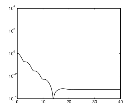
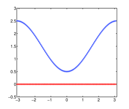
Refer to caption Refer to caption (a)π‘Ž\displaystyle(a) (b)𝑏\displaystyle(b) t𝑑\displaystyle t xπ‘₯\displaystyle x

Figure 4: Numerical solutions of (79) with the distance from the asymptotic solution (90) in (a)π‘Ž\displaystyle(a) and the fields at t=100𝑑100\displaystyle t=100 in (b)𝑏\displaystyle(b). Here a=1.5π‘Ž1.5\displaystyle a=1.5, Ξ΅=0.01πœ€0.01\displaystyle\varepsilon=0.01 and the discretisation is Δ​x=2​π/100Ξ”π‘₯2πœ‹100\displaystyle\Delta x=2\pi/100 and Δ​t=1Γ—10βˆ’3Δ𝑑1superscript103\displaystyle\Delta t=1\times 10^{-3}.

Refer to caption Refer to caption (a)π‘Ž\displaystyle(a) (b)𝑏\displaystyle(b) t𝑑\displaystyle t xπ‘₯\displaystyle x

Figure 5: t Numerical solutions of (79) with the distance from the asymptotic solution (90) in (a)π‘Ž\displaystyle(a) and the fields at t=12.5𝑑12.5\displaystyle t=12.5 in (b)𝑏\displaystyle(b). Here a=0.5π‘Ž0.5\displaystyle a=0.5, Ξ΅=0.01πœ€0.01\displaystyle\varepsilon=0.01 and the discretisation is Δ​x=2​π/100Ξ”π‘₯2πœ‹100\displaystyle\Delta x=2\pi/100 and Δ​t=1Γ—10βˆ’3Δ𝑑1superscript103\displaystyle\Delta t=1\times 10^{-3}. The vertical dashed line in (a)π‘Ž\displaystyle(a) is the first time that u=0𝑒0\displaystyle u=0.

If Ξ΅=0πœ€0\displaystyle{\varepsilon}=0 and with initial conditions

u​(x,0)=a,v​(x,0)=βˆ’sin⁑(x)/2,formulae-sequence𝑒π‘₯0π‘Žπ‘£π‘₯0π‘₯2u(x,0)=a\,,\qquad v(x,0)=-\sin(x)/2\,, (87)

the (linear) equations (79) have the exact solution

u​(x,t)=eβˆ’t/22​[cos⁑(x+3​t/2)+cos⁑(xβˆ’3​t/2)]+aβˆ’cos⁑xv​(x,t)=eβˆ’t/22​[cos⁑(x+3​t/2+Ο€/6)βˆ’cos⁑(xβˆ’3​t/2βˆ’Ο€/6)].𝑒π‘₯𝑑superscript𝑒𝑑22delimited-[]π‘₯3𝑑2π‘₯3𝑑2π‘Žπ‘₯𝑣π‘₯𝑑superscript𝑒𝑑22delimited-[]π‘₯3𝑑2πœ‹6π‘₯3𝑑2πœ‹6\begin{array}[]{ccl}u(x,t)&=&\frac{e^{-t/2}}{2}[\cos(x+\sqrt{3}t/2)+\cos(x-\sqrt{3}t/2)]+a-\cos x\\ v(x,t)&=&\frac{e^{-t/2}}{2}[\cos(x+\sqrt{3}t/2+\pi/6)-\cos(x-\sqrt{3}t/2-\pi/6)]\,.\end{array} (88)

The large-time limit of these solutions,

u​(x,∞)=aβˆ’cos⁑x,v​(x,∞)=0,formulae-sequence𝑒π‘₯π‘Žπ‘₯𝑣π‘₯0u(x,\infty)=a-\cos x\,,\qquad v(x,\infty)=0\,, (89)

is also a steady-state solution of the nonlinear system (with Ξ΅>0πœ€0\displaystyle{\varepsilon}>0). If a>1π‘Ž1\displaystyle a>1, then u​(x,∞)>0𝑒π‘₯0\displaystyle u(x,\infty)>0, and the calculations above suggest that the equations will be linearly well-posed. However if a<1π‘Ž1\displaystyle a<1, then u​(x,∞)𝑒π‘₯\displaystyle u(x,\infty) dips below zero over an interval, which suggests that the equations will be ill-posed.

FigureΒ 5, where a=1.5π‘Ž1.5\displaystyle a=1.5, and FigureΒ 5, where a=0.5π‘Ž0.5\displaystyle a=0.5, confirm these expectations. They show numerical solutions using a central-space forward-time explicit scheme on the periodic domain x∈[βˆ’Ο€,Ο€]π‘₯πœ‹πœ‹\displaystyle x\in[-\pi,\pi] with a spatial resolution of Δ​x=2​π/100Ξ”π‘₯2πœ‹100\displaystyle\Delta x=2\pi/100. Each figure has two panels, one showing the temporal evolution of the distance from the asymptotic solution,

Dist=max⁑{|uβˆ’u​(x,∞)|2+|vβˆ’v​(x,∞)|2},Distsuperscript𝑒𝑒π‘₯2superscript𝑣𝑣π‘₯2\mbox{Dist}=\max\left\{\sqrt{|u-u(x,\infty)|^{2}+|v-v(x,\infty)|^{2}}\right\}\,, (90)

and the other plotting the two variables u,v𝑒𝑣\displaystyle u,v at a specific (late) time during the computation. In Figure 5, the well posed case, the numerical solution converges to the predicted steady state solution (89) within numerical accuracy. By contrast, in FigureΒ 5, after an initial decay, ill-posedness asserts itself and causes the solution to blow up.
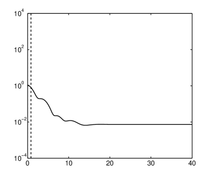
Refer to caption Refer to caption (a)π‘Ž\displaystyle(a) (b)𝑏\displaystyle(b) t𝑑\displaystyle t xπ‘₯\displaystyle x

Figure 6: Numerical solutions of (79) with the distance from the asymptotic solution (90) in (a)π‘Ž\displaystyle(a) and the fields at t=100𝑑100\displaystyle t=100 in (b)𝑏\displaystyle(b). Here a=0.5π‘Ž0.5\displaystyle a=0.5, Ξ΅=0.01πœ€0.01\displaystyle\varepsilon=0.01 and the discretisation is Δ​x=2​π/30Ξ”π‘₯2πœ‹30\displaystyle\Delta x=2\pi/30 and Δ​t=1Γ—10βˆ’3Δ𝑑1superscript103\displaystyle\Delta t=1\times 10^{-3}. The vertical dashed line is the first time that u=0𝑒0\displaystyle u=0.

Regarding grid dependence, FigureΒ 6 shows another computation in the ill posed case with a coarser grid, Δ​x=2​π/30Ξ”π‘₯2πœ‹30\displaystyle\Delta x=2\pi/30. The solution appears to converge to the steady state solution, just like in the well posed case. In other words, the computations on the coarse grid hide the ill posed character of the underlying PDEs. This highlights that in order to extract meaningful information from numerical computations, a proper study of grid convergence must be first carried out.

Incidentally, if the grid is made finer than in FiguresΒ 5 and 5, in the well posed case a>1π‘Ž1\displaystyle a>1 the numerical solution converges to the steady-state solution with a smaller numerical error, while in the ill-posed case it blows up sooner, as expected.

Acknowledgements

This research was supported by NERC grants NE/E003206/1 and NE/K003011/1 as well as EPSRC grants EP/I019189/1, EP/K00428X/1 and EP/M022447/1. J.M.N.T.G. is a Royal Society Wolfson Research Merit Award holder (WM150058) and an EPSRC Established Career Fellow (EP/M022447/1). Research of M.S. was supported by National Science Foundation grant DMS-1517291.

References

  • [1] Jackson R. Some mathematical and physical aspects of continuum models for the motion of the granular materials. In Theory of dispersed multiphase flow. R. Meyer, Academic Press; 1983.
  • [2] Schaeffer D. Instability in the evolution-equations describing incompressible granular flow. J Differ Equ. 1987;66(1):19–50.
  • [3] Schaeffer DG, Pitman EB. Ill-posedness in three-dimensional plastic flow. Comm Pure Appl Math. 1988;41(7):879–890.
  • [4] GDR MiDi. On dense granular flows. Eur Phys J E. 2004;14(4):341–365.
  • [5] Jop P, Forterre Y, Pouliquen O. A constitutive relation for dense granular flows. Nature. 2006;44:727–730.
  • [6] Joseph DD, Saut JC. Short-wave instabilities and ill-posed initial-value problems. Theor Comput Fluid Dyn. 1990;1:191–227.
  • [7] Gray JMNT. Loss of hyperbolicity and ill-posedness of the viscous-plastic sea ice rheology in uniaxial divergent flow. J Phys Oceanog. 1999 NOV;29(11):2920–2929.
  • [8] Woodhouse MJ, Thornton AR, Johnson CG, Kokelaar BP, Gray JMNT. Segregation-induced fingering instabilities in granular free-surface flows. J Fluid Mech. 2012;709:543–580.
  • [9] Barker T, Schaeffer DG, Bohorquez P, Gray JMNT. Well-posed and ill-posed behaviour of the mu(I)-rheology for granular flow. J Fluid Mech. 2015;779:794–818.
  • [10] Mandel J. Conditions de stabilitΓ© et postulate de Drucker. Rheology and Soil Mechanics, eds Kravtchenko, G and Sirieys,P. 1964;p. 58–68.
  • [11] Pitman EB, Schaeffer DG. Stability of time dependent compressible granular flow in two dimensions. Communications on Pure and Applied Mathematics. 1987;40(4):421–447.
  • [12] deΒ Coulomb CA. Essai sur une application des r gles de maximis & minimis quelques probl mes de statique, relatifs l’architecture. Mem Math Acad R Sci, Paris. 1773;7:343–382.
  • [13] daΒ Cruz F, Emam S, Prochnow M, Roux J, Chevoir F. Rheophysics of dense granular materials: Discrete simulation of plane shear flows. Phys Rev E. 2005;72:021309.
  • [14] Pitman EB. The stability of granular flow in converging hoppers. SIAM Journal On Applied Mathematics. 1988;48:1033–1053.
  • [15] Kamrin K. Nonlinear elasto-plastic model for dense granular flow. Int J Plasticity. 2010;26:167–188.
  • [16] Jiang Y, Liu M. From elasticity to hypoplasticity: dynamics of granular solids. Physical review letters. 2007;99(10):105501.
  • [17] Pouliquen O, Forterre Y. A non-local rheology for dense granular flows. Phil Trans R Soc A. 2009;367:5091–5107.
  • [18] Kamrin K, Koval G. Nonlocal constitutive relation for steady granular flow. Phys Rev Lett. 2012;108(17):178301.
  • [19] Kamrin K, Henann D. Nonlocal Modeling of Granular Flows Down Inclines. Soft Matter. 2015;11(1):179–185.
  • [20] Bouzid M, Trulsson M, Claudin P, ClΓ©ment E, Andreotti B. Nonlocal Rheology of Granular Flows across Yield Conditions. Phys Rev Lett. 2013;111(23):238301.
  • [21] Jenkins JT, Savage SB. A theory for the rapid flow of identical, smooth, nearly elastic, spherical-particles. J Fluid Mech. 1983;130:187–202.
  • [22] Harris D, Grekova EF. A hyperbolic well-posed model for the flow of granular materials. J Eng Math. 2005;52:107–135.
  • [23] Sun J, Sundaresan S. A constitutive model with microstructure evolution for flow of rate-independent granular materials. J Fluid Mech. 2011;682:590–616.
  • [24] Wu W, Bauer E, Kolymbas D. Hypoplastic constitutive model with critical state for granular materials. Mech Mater. 1996;23(1):45–69.
  • [25] Perzyna P. Fundamental problems in viscoplasticity. Advances in applied mechanics. 1966;9:243–377.
  • [26] Jop P, Forterre Y, Pouliquen O. Crucial role of sidewalls in granular surface flows: consequences for the rheology. J Fluid Mech. 2005;541:167.
  • [27] Pinchover Y, Rubinstein J. An Introduction to partial differential equations. Cambridge University Press; 2005.
  • [28] Kreiss HO. Numerical methods for solving time-dependent problems for partial differential equations. Presses Univ. MontrΓ©al; 1978.