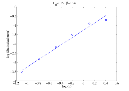
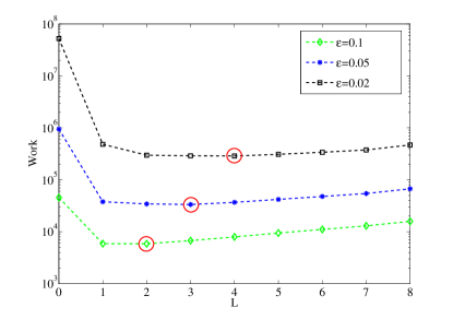
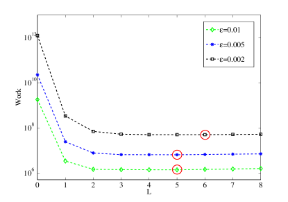
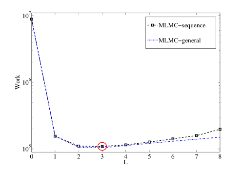
The optimal multilevel Monte-Carlo approximation of the stochastic drift-diffusion-Poisson system

Leila Taghizadeh Leila.Taghizadeh@TUWien.ac.at Amirreza Khodadadian Amirreza.Khodadadian@TUWien.ac.at Clemens Heitzinger Clemens.Heitzinger@TUWien.ac.at Institute for Analysis and Scientific Computing, Vienna University of Technology (TU Wien), Wiedner Hauptstraße 8–10, 1040 Vienna, Austria School of Mathematical and Statistical Sciences, Arizona State University, Tempe, AZ 85287, USA
Abstract

Existence and local-uniqueness theorems for weak solutions of a system consisting of the drift-diffusion-Poisson equations and the Poisson-Boltzmann equation, all with stochastic coefficients, are presented. For the numerical approximation of the expected value of the solution of the system, we develop a multi-level Monte-Carlo (MLMC) finite-element method (FEM) and we analyze its rate of convergence and its computational complexity. This allows to find the optimal choice of discretization parameters. Finally, numerical results show the efficiency of the method. Applications are, among others, noise and fluctuations in nanoscale transistors, in field-effect bio- and gas sensors, and in nanopores.

keywords:
Stochastic drift-diffusion-Poisson system, existence and uniqueness, multi-level Monte-Carlo finite-element method, optimal method.

1 Introduction

In this work, we consider the system consisting of the drift-diffusion-Poisson equations coupled with the Poisson-Boltzmann equation, all with random coefficients. We show existence and local uniqueness of weak solutions for the stationary problem. This system is a general model for transport processes, where a stochastic process determines the coefficients. Furthermore, we develop a multi-level (ML) Monte-Carlo (MC) finite-element method (FEM) for the system of equations. The different types of errors in the numerical approximation must be balanced and the optimal approach is found here.

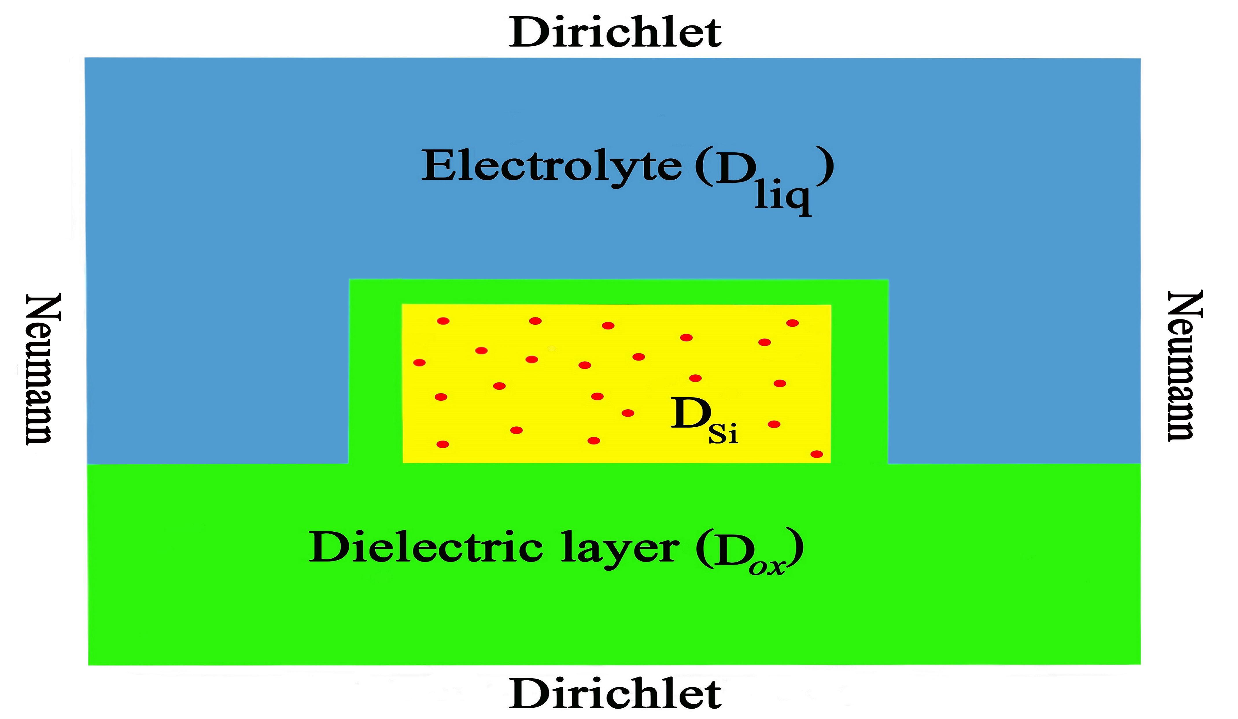
In the system of equations considered here, both the operators and the forcing terms are stochastic, and therefore this system has numerous applications (see Figure 1). A deterministic and simplified version, without the Poisson-Boltzmann equation, is the standard model for semiconductor devices. Nowadays, randomness due to the location of impurity atoms is the most important effect limiting the design of integrated circuits. This application area is included in the present model equations. Furthermore, the full system of equations considered here describes a very general class of field-effect sensors including their most recent incarnation, nanowire bio- and gas sensors. While previous mathematical modeling has focused on the deterministic problem and stochastic surface reactions [1, 2, 3, 4, 5, 6], the present model describes how various stochastic processes propagate through a PDE model and result in noise and fluctuations in a transport model. Quantifying noise and fluctuations in sensors is important, since they determine the detection limit and the signal-to-noise ratio. Noise and fluctuations are of great importance especially in nanometer-scale devices, as any random effect becomes proportionally more important as devices are shrunk.

Various sources of noise and fluctuations are included in the model equations here. Doping of semiconductor devices is inherently random and results in a random number of impurity atoms placed at random positions, each one changing the charge concentration and the mobility at its location. In field-effect sensors, target molecules bind to randomly placed probe molecules in a stochastic process, so that the detection mechanism is inherently stochastic. The Brownian motion of the target molecules also results in changes in charge concentration and permittivity. This randomness at the sensor surface propagates through the self-consistent transport equations and finally results in noise in the sensor output.

In summary, there are many applications where both the operators and the forcing terms in the drift-diffusion-Poisson system are random. The probability distributions of permittivities and charge concentrations can be calculated from physical models [7].
Refer to caption
Figure 1: Schematic diagram showing leading applications. In a field-effect transistor, the dopant atoms are randomly distributed (there is no electrolyte). In field-effect sensors, there are randomly distributed dopant atoms as well as randomly distributed charged molecules in the electrolyte.

In many realistic situations, the probability space is high-dimensional. For example, each probe molecule, each target molecule, and each probe-target complex needs to be modeled in sensors. In transistors, the number impurities and their positions are random. The large number of dimensions favors the use of Monte-Carlo (MC) methods: It is well-known that the convergence rate of standard MC methods is independent of the number of dimensions. On the other hand, it is inversely proportional to the square root of the number of evaluations and here each evaluation requires solving a two- or three-dimensional system of elliptic equations.

These considerations motivate the development of a multi-level Monte-Carlo (MLMC) algorithm. In [8], after earlier work [9] on numerical quadrature, it was shown that a multi-level approach and a geometric sequence of timesteps can reduce the order of computational complexity of MC path simulations for estimating the expected value of the solution of a stochastic ordinary differential equation. This is done by reducing the variance and leaving the bias unchanged due to the Euler discretization used as the ODE solver. In [10], the Milstein scheme was used as the ODE solver to improve the convergence rate of the MLMC method for scalar stochastic ordinary differential equations and the method was made more efficient. The new method has the same weak order of convergence, but an improved first-order strong convergence, and it is the strong order of convergence which is central to the efficiency of MLMC methods. In [11], the MLMC method was combined with quasi-Monte-Carlo (QMC) integration using a randomized rank-1 lattice rule and the asymptotic order of convergence of MLMC was improved and a lower computational cost was achieved as well.

In [12], an MLMC finite-element method was presented for elliptic partial differential equations with stochastic coefficients. In this problem, the source of randomness lies in the coefficients inside the operator and the coefficient fields are bounded uniformly from above and away from zero. The MLMC error and work estimates were given for the expected values of the solutions and for higher moments. Also, in [13], the same problem was considered and numerical results indicate that the MLMC estimator is not limited to smooth problems. In [14], a multi-level quasi-Monte-Carlo finite-element method for a class of elliptic PDEs with random coefficients was presented. The error analysis of QMC was generalized to a multi-level scheme with the number of QMC points dependent on the discretization level and with a level-dependent dimension truncation strategy.

In [15], uniform bounds on the finite-element error were shown in standard Bochner spaces. These new bounds can be used to perform a rigorous analysis of the MLMC method for elliptic problems, and a rigorous bound on the MLMC complexity in a more general case was found. In [16], the finite-element error analysis was extended for the same type of equations posed on non-smooth domains and with discontinuities in the coefficient. In [17], a general optimization of the parameters in the MLMC discretization hierarchy based on uniform discretization methods with general approximation orders and computational costs was developed. In current work, we define a global optimization problem which minimizes the computational complexity such that the error bound is less or equal to a given tolerance level.

The rest of this paper is organized as follows. In Section 2, we present the system of model equations with stochastic coefficients in detail. In Section 3, we define weak solutions of the model equations and prove existence and local-uniqueness theorems. Section 4.1 collects results about the FEM for later use. In Section 4, we introduce a multi-level Monte-Carlo finite-element method for the system and analyze its rate of convergence. In Section 5, we discuss the computational complexity and find the optimal MLMC method. In Section 6, we present numerical results for random impurity atoms in nanowire field-effect sensors. The MLMC-FEM method is illustrated there and the computational costs of various numerical techniques are compared as well. Finally, conclusions are drawn in Section 7.

2 The Stochastic Model Equations

Suppose that the domain Dd𝐷superscript𝑑D\subset\mathbb{R}^{d} is bounded and convex, and that d3𝑑3d\leq 3. The whole domain D𝐷D is partitioned into three subdomains with different physical properties and hence different model equations in order to include a large range of applications. The first subdomain DSisubscript𝐷SiD_{\mathrm{Si}} consists of the (silicon) nanowire and acts as the transducer of the sensor; in this subdomain, the drift-diffusion-Poisson system describes charge transport. The semiconductor is surrounded by a dielectric layer (usually an oxide) which comprises the second subdomain Doxsubscript𝐷oxD_{\mathrm{ox}}, where just the Poisson equation holds. Finally, the third subdomain Dliqsubscript𝐷liqD_{\mathrm{liq}} is the aqueous solution containing cations and anions and the Poisson-Boltzmann equation holds. Also, the boundary layer at the sensor surface is responsible for the recognition of the target molecules. In the case of field-effect sensors, solving a homogenization problem gives rise to two interface conditions for the Poisson equation [1]. In summary, the domain is partitioned into

D=DSiDoxDliq.𝐷subscript𝐷Sisubscript𝐷oxsubscript𝐷liqD=D_{\mathrm{Si}}\cup D_{\mathrm{ox}}\cup D_{\mathrm{liq}}.

In the subdomain DSisubscript𝐷SiD_{\mathrm{Si}}, the stationary drift-diffusion-Poisson system

(A(x,ω)V(x,ω))𝐴𝑥𝜔𝑉𝑥𝜔\displaystyle-\nabla\cdot(A(x,\omega)\nabla V(x,\omega)) =q(Cdop(x,ω)+p(x,ω)n(x,ω)),absent𝑞subscript𝐶dop𝑥𝜔𝑝𝑥𝜔𝑛𝑥𝜔\displaystyle=q(C_{\mathrm{dop}}(x,\omega)+p(x,\omega)-n(x,\omega)), (1a)
Jn(x,ω)subscript𝐽𝑛𝑥𝜔\displaystyle\nabla\cdot J_{n}(x,\omega) =qR(n(x,ω),p(x,ω)),absent𝑞𝑅𝑛𝑥𝜔𝑝𝑥𝜔\displaystyle=qR(n(x,\omega),p(x,\omega)), (1b)
Jp(x,ω)subscript𝐽𝑝𝑥𝜔\displaystyle\nabla\cdot J_{p}(x,\omega) =qR(n(x,ω),p(x,ω)),absent𝑞𝑅𝑛𝑥𝜔𝑝𝑥𝜔\displaystyle=-qR(n(x,\omega),p(x,\omega)), (1c)
Jn(x,ω)subscript𝐽𝑛𝑥𝜔\displaystyle J_{n}(x,\omega) =q(Dnn(x,ω)μnn(x,ω)V(x,ω)),absent𝑞subscript𝐷𝑛𝑛𝑥𝜔subscript𝜇𝑛𝑛𝑥𝜔𝑉𝑥𝜔\displaystyle=q(D_{n}\nabla n(x,\omega)-\mu_{n}n(x,\omega)\nabla V(x,\omega)), (1d)
Jp(x,ω)subscript𝐽𝑝𝑥𝜔\displaystyle J_{p}(x,\omega) =q(Dpp(x,ω)μpp(x,ω)V(x,ω))absent𝑞subscript𝐷𝑝𝑝𝑥𝜔subscript𝜇𝑝𝑝𝑥𝜔𝑉𝑥𝜔\displaystyle=q(-D_{p}\nabla p(x,\omega)-\mu_{p}p(x,\omega)\nabla V(x,\omega)) (1e)

models charge transport, where A(x,ω)𝐴𝑥𝜔A(x,\omega), the permittivity, is a random field with xd𝑥superscript𝑑x\in\mathbb{R}^{d} and a random parameter ωΩ𝜔Ω\omega\in\Omega in a probability space (Ω,𝔸,)Ω𝔸(\Omega,\mathbb{A},\mathbb{P}). ΩΩ\Omega denotes the set of elementary events, i.e., the sample space, 𝔸𝔸\mathbb{A} the σ𝜎\sigma-algebra of all possible events, and :𝔸[0,1]:𝔸01\mathbb{P}\colon\mathbb{A}\to[0,1] is a probability measure. V(x,ω)𝑉𝑥𝜔V(x,\omega) is the electrostatic potential and q>0𝑞0q>0 is the elementary charge, Cdop(x,ω)subscript𝐶dop𝑥𝜔C_{\mathrm{dop}}(x,\omega) is the doping concentration, n(x,ω)𝑛𝑥𝜔n(x,\omega) and p(x,ω)𝑝𝑥𝜔p(x,\omega) are the concentrations of electrons and holes, respectively, Jn(x,ω)subscript𝐽𝑛𝑥𝜔J_{n}(x,\omega) and Jp(x,ω)subscript𝐽𝑝𝑥𝜔J_{p}(x,\omega) are the current densities, Dnsubscript𝐷𝑛D_{n} and Dpsubscript𝐷𝑝D_{p} are the diffusion coefficients, μnsubscript𝜇𝑛\mu_{n} and μpsubscript𝜇𝑝\mu_{p} are the mobilities, and R(n(x,ω),p(x,ω))𝑅𝑛𝑥𝜔𝑝𝑥𝜔R(n(x,\omega),p(x,\omega)) is the recombination rate. We use the Shockley-Read-Hall recombination rate

R(n(x,ω),p(x,ω)):=n(x,ω)p(x,ω)ni2τp(n(x,ω)+ni)+τn(p(x,ω)+ni)assign𝑅𝑛𝑥𝜔𝑝𝑥𝜔𝑛𝑥𝜔𝑝𝑥𝜔superscriptsubscript𝑛𝑖2subscript𝜏𝑝𝑛𝑥𝜔subscript𝑛𝑖subscript𝜏𝑛𝑝𝑥𝜔subscript𝑛𝑖R(n(x,\omega),p(x,\omega)):=\frac{n(x,\omega)p(x,\omega)-n_{i}^{2}}{\tau_{p}(n(x,\omega)+n_{i})+\tau_{n}(p(x,\omega)+n_{i})}

here, where the constant nisubscript𝑛𝑖n_{i} is the intrinsic charge density and τnsubscript𝜏𝑛\tau_{n} and τpsubscript𝜏𝑝\tau_{p} are the lifetimes of the free carriers, although the mathematical results here hold for many expressions for the recombination rate. Equations (1) include the convection terms nV𝑛𝑉-n\nabla V and pV𝑝𝑉-p\nabla V, which prohibit the use of the maximum principle in a simple way.

We assume that the Einstein relations Dn=UTμnsubscript𝐷𝑛subscript𝑈𝑇subscript𝜇𝑛D_{n}=U_{T}\mu_{n} and Dp=UTμpsubscript𝐷𝑝subscript𝑈𝑇subscript𝜇𝑝D_{p}=U_{T}\mu_{p} hold, where the constant UTsubscript𝑈𝑇U_{T} is the thermal voltage. Therefore, it is beneficial to change variables from the concentrations n𝑛n and p𝑝p to the Slotboom variables u𝑢u and v𝑣v defined by

n(x,ω)𝑛𝑥𝜔\displaystyle n(x,\omega) =:nieV(x,ω)/UTu(x,ω),\displaystyle=:n_{i}\mathrm{e}^{V(x,\omega)/U_{T}}u(x,\omega),
p(x,ω)𝑝𝑥𝜔\displaystyle p(x,\omega) =:nieV(x,ω)/UTv(x,ω).\displaystyle=:n_{i}\mathrm{e}^{-V(x,\omega)/U_{T}}v(x,\omega).

The system (1) then becomes

(AV(x,ω))𝐴𝑉𝑥𝜔\displaystyle-\nabla\cdot(A\nabla V(x,\omega)) =qni(eV(x,ω)/UTv(x,ω)eV(x,ω)/UTu(x,ω))+qCdop(x,ω),absent𝑞subscript𝑛𝑖superscript𝑒𝑉𝑥𝜔subscript𝑈𝑇𝑣𝑥𝜔superscript𝑒𝑉𝑥𝜔subscript𝑈𝑇𝑢𝑥𝜔𝑞subscript𝐶dop𝑥𝜔\displaystyle=qn_{i}(e^{-V(x,\omega)/U_{T}}v(x,\omega)-e^{V(x,\omega)/U_{T}}u(x,\omega))+qC_{\mathrm{dop}}(x,\omega),
UT(μneV(x,ω)/UTu(x,ω))subscript𝑈𝑇subscript𝜇𝑛superscript𝑒𝑉𝑥𝜔subscript𝑈𝑇𝑢𝑥𝜔\displaystyle U_{T}\nabla\cdot(\mu_{n}e^{V(x,\omega)/U_{T}}\nabla u(x,\omega)) =u(x,ω)v(x,ω)1τp(eV(x,ω)/UTu(x,ω)+1)+τn(eV(x,ω)/UTv(x,ω)+1),absent𝑢𝑥𝜔𝑣𝑥𝜔1subscript𝜏𝑝superscript𝑒𝑉𝑥𝜔subscript𝑈𝑇𝑢𝑥𝜔1subscript𝜏𝑛superscript𝑒𝑉𝑥𝜔subscript𝑈𝑇𝑣𝑥𝜔1\displaystyle=\frac{u(x,\omega)v(x,\omega)-1}{\tau_{p}(e^{V(x,\omega)/U_{T}}u(x,\omega)+1)+\tau_{n}(e^{-V(x,\omega)/U_{T}}v(x,\omega)+1)},
UT(μpeV(x,ω)/UTv(x,ω))subscript𝑈𝑇subscript𝜇𝑝superscript𝑒𝑉𝑥𝜔subscript𝑈𝑇𝑣𝑥𝜔\displaystyle U_{T}\nabla\cdot(\mu_{p}e^{-V(x,\omega)/U_{T}}\nabla v(x,\omega)) =u(x,ω)v(x,ω)1τp(eV(x,ω)/UTu(x,ω)+1)+τn(eV(x,ω)/UTv(x,ω)+1),absent𝑢𝑥𝜔𝑣𝑥𝜔1subscript𝜏𝑝superscript𝑒𝑉𝑥𝜔subscript𝑈𝑇𝑢𝑥𝜔1subscript𝜏𝑛superscript𝑒𝑉𝑥𝜔subscript𝑈𝑇𝑣𝑥𝜔1\displaystyle=\frac{u(x,\omega)v(x,\omega)-1}{\tau_{p}(e^{V(x,\omega)/U_{T}}u(x,\omega)+1)+\tau_{n}(e^{-V(x,\omega)/U_{T}}v(x,\omega)+1)},

where the continuity equations are self-adjoint.

The boundary D𝐷\partial D is partitioned into Dirichlet and Neumann boundaries. For the Ohmic contacts we have

V(x,ω)|DD=VD(x),u(x,ω)|DSi,D=uD(x)andv(x,ω)|DSi,D=vD(x).formulae-sequenceevaluated-at𝑉𝑥𝜔subscript𝐷𝐷subscript𝑉𝐷𝑥formulae-sequenceevaluated-at𝑢𝑥𝜔subscript𝐷Si𝐷subscript𝑢𝐷𝑥andevaluated-at𝑣𝑥𝜔subscript𝐷Si𝐷subscript𝑣𝐷𝑥V(x,\omega)|_{\partial D_{D}}=V_{D}(x),\quad u(x,\omega)|_{\partial D_{\mathrm{Si},D}}=u_{D}(x)\quad\text{and}\quad v(x,\omega)|_{\partial D_{\mathrm{Si},D}}=v_{D}(x).

At Ohmic contacts the space charge vanishes, i.e., Cdop+pDnD=0subscript𝐶dopsubscript𝑝𝐷subscript𝑛𝐷0C_{\mathrm{dop}}+p_{D}-n_{D}=0, and the system is in thermal equilibrium, i.e., nDpD=ni2subscript𝑛𝐷subscript𝑝𝐷superscriptsubscript𝑛𝑖2n_{D}p_{D}=n_{i}^{2} on DDsubscript𝐷𝐷\partial D_{D}. Furthermore, at each contact, the quasi Fermi potential levels of silicon are aligned with an external applied voltage U(x)𝑈𝑥U(x). Therefore, by using the quasi Fermi potential, we determine the boundary condition on DSi,Dsubscript𝐷Si𝐷\partial D_{\mathrm{Si},D} using

V1(x):=U(x)+UTln(nD(x)ni)=U(x)UTln(pD(x)ni).assignsubscript𝑉1𝑥𝑈𝑥subscript𝑈𝑇subscript𝑛𝐷𝑥subscript𝑛𝑖𝑈𝑥subscript𝑈𝑇subscript𝑝𝐷𝑥subscript𝑛𝑖V_{1}(x):=U(x)+U_{T}\ln\left(\frac{n_{D}(x)}{n_{i}}\right)=U(x)-U_{T}\ln\left(\frac{p_{D}(x)}{n_{i}}\right).

The boundary values uD(x)subscript𝑢𝐷𝑥u_{D}(x) and vD(x)subscript𝑣𝐷𝑥v_{D}(x) are found to be

uD(x)subscript𝑢𝐷𝑥\displaystyle u_{D}(x) :=ni1eV1(x)/UTnD(x),assignabsentsuperscriptsubscript𝑛𝑖1superscript𝑒subscript𝑉1𝑥subscript𝑈𝑇subscript𝑛𝐷𝑥\displaystyle:=n_{i}^{-1}e^{-V_{1}(x)/U_{T}}n_{D}(x),
vD(x)subscript𝑣𝐷𝑥\displaystyle v_{D}(x) :=ni1eV1(x)/UTpD(x),assignabsentsuperscriptsubscript𝑛𝑖1superscript𝑒subscript𝑉1𝑥subscript𝑈𝑇subscript𝑝𝐷𝑥\displaystyle:=n_{i}^{-1}e^{V_{1}(x)/U_{T}}p_{D}(x),

where

nD(x)subscript𝑛𝐷𝑥\displaystyle n_{D}(x) :=12(Cdop+Cdop2+4ni2),assignabsent12subscript𝐶dopsuperscriptsubscript𝐶dop24superscriptsubscript𝑛𝑖2\displaystyle:=\frac{1}{2}\left(C_{\mathrm{dop}}+\sqrt{C_{\mathrm{dop}}^{2}+4n_{i}^{2}}\right),
pD(x)subscript𝑝𝐷𝑥\displaystyle p_{D}(x) :=12(Cdop+Cdop2+4ni2)assignabsent12subscript𝐶dopsuperscriptsubscript𝐶dop24superscriptsubscript𝑛𝑖2\displaystyle:=\frac{1}{2}\left(-C_{\mathrm{dop}}+\sqrt{C_{\mathrm{dop}}^{2}+4n_{i}^{2}}\right)

hold [18, Chapter 3]. Here, Cdop:=ND+NAassignsubscript𝐶dopsuperscriptsubscript𝑁𝐷superscriptsubscript𝑁𝐴C_{\mathrm{dop}}:=N_{D}^{+}-N_{A}^{-} is the net doping concentration, where ND+superscriptsubscript𝑁𝐷N_{D}^{+} and NAsuperscriptsubscript𝑁𝐴N_{A}^{-} are the donor and acceptor concentrations, respectively.

The zero Neumann boundary conditions

𝐧V(x,ω)=0,𝐧u(x,ω)=0,𝐧v(x,ω)=0formulae-sequence𝐧𝑉𝑥𝜔0formulae-sequence𝐧𝑢𝑥𝜔0𝐧𝑣𝑥𝜔0\mathbf{n}\cdot\nabla V(x,\omega)=0,\quad\mathbf{n}\cdot\nabla u(x,\omega)=0,\quad\mathbf{n}\cdot\nabla v(x,\omega)=0

hold on the rest of the boundary D𝐷\partial D. Here 𝐧𝐧\mathbf{n} denotes the unit outward normal vector on the boundary.

A jump in the permittivity A𝐴A always gives rise to two continuity conditions: the continuity of the potential and the continuity of the electric displacement field. Homogenization of an elliptic problem with a periodic boundary layer at a manifold ΓΓ\Gamma yields the two interface conditions [1]

V(0+,y,ω)V(0,y,ω)𝑉limit-from0𝑦𝜔𝑉limit-from0𝑦𝜔\displaystyle V(0+,y,\omega)-V(0-,y,\omega) =α(y,ω),absent𝛼𝑦𝜔\displaystyle=\alpha(y,\omega),
A(0+)xV(0+,y,ω)A(0)xV(0,y,ω)𝐴limit-from0subscript𝑥𝑉limit-from0𝑦𝜔𝐴limit-from0subscript𝑥𝑉limit-from0𝑦𝜔\displaystyle A(0+)\partial_{x}V(0+,y,\omega)-A(0-)\partial_{x}V(0-,y,\omega) =γ(y,ω)absent𝛾𝑦𝜔\displaystyle=\gamma(y,\omega)

between the semiconductor and the liquid. Here we denote the one-dimensional coordinate orthogonal to the manifold ΓΓ\Gamma by x𝑥x and the remaining (d1)𝑑1(d-1)-dimensional coordinates by y𝑦y. α𝛼\alpha and γ𝛾\gamma are essentially given by the dipole-moment and the surface-charge densities of the boundary layer; in general, we write them as the functional Mα(V)subscript𝑀𝛼𝑉M_{\alpha}(V) and Mγ(V)subscript𝑀𝛾𝑉M_{\gamma}(V) of the potential V𝑉V. They may correspond to the Metropolis Monte-Carlo method [19], to solving the nonlinear Poisson-Boltzmann equation [7], or to systems of ordinary differential equations for surface reactions [20, 21].

In the subdomain Doxsubscript𝐷oxD_{\mathrm{ox}}, there are no charge carriers and the Poisson equation is simply

(AV(x,ω))=0.𝐴𝑉𝑥𝜔0-\nabla\cdot(A\nabla V(x,\omega))=0.

In the subdomain Dliqsubscript𝐷liqD_{\mathrm{liq}}, the nonlinear Poisson-Boltzmann equation

(A(x,ω)V(x,ω))+2ηsinh(β(V(x,ω)Φ(x,ω)))=0𝐴𝑥𝜔𝑉𝑥𝜔2𝜂𝛽𝑉𝑥𝜔Φ𝑥𝜔0-\nabla\cdot(A(x,\omega)\nabla V(x,\omega))+2\eta\sinh(\beta(V(x,\omega)-\Phi(x,\omega)))=0

holds and models screening by free charges. Here η𝜂\eta is the ionic concentration, the constant β𝛽\beta equals β:=q/(kBT)assign𝛽𝑞subscript𝑘𝐵𝑇\beta:=q/(k_{B}T) in terms of the Boltzmann constant kBsubscript𝑘𝐵k_{B} and the temperature T𝑇T, and ΦΦ\Phi is the Fermi level.

In summary, for all ωΩ𝜔Ω\omega\in\Omega, the model equations are the boundary-value problem

(A(x,ω)V(x,ω))𝐴𝑥𝜔𝑉𝑥𝜔\displaystyle-\nabla\cdot(A(x,\omega)\nabla V(x,\omega)) (2a)
=qCdop(x,ω)qni(eV(x,ω)/UTu(x,ω)eV(x,ω)/UTv(x,ω))absent𝑞subscript𝐶dop𝑥𝜔𝑞subscript𝑛𝑖superscripte𝑉𝑥𝜔subscript𝑈𝑇𝑢𝑥𝜔superscripte𝑉𝑥𝜔subscript𝑈𝑇𝑣𝑥𝜔\displaystyle=qC_{\mathrm{dop}}(x,\omega)-qn_{i}(\mathrm{e}^{V(x,\omega)/U_{T}}u(x,\omega)-\mathrm{e}^{-V(x,\omega)/U_{T}}v(x,\omega)) in DSi,in subscript𝐷Si\displaystyle\text{in }D_{\mathrm{Si}},
(A(x,ω)V(x,ω))=0𝐴𝑥𝜔𝑉𝑥𝜔0\displaystyle-\nabla\cdot(A(x,\omega)\nabla V(x,\omega))=0 in Dox,in subscript𝐷ox\displaystyle\text{in }D_{\mathrm{ox}}, (2b)
(A(x,ω)V(x,ω))=2ηsinh(β(V(x,ω)Φ(x,ω)))𝐴𝑥𝜔𝑉𝑥𝜔2𝜂𝛽𝑉𝑥𝜔Φ𝑥𝜔\displaystyle-\nabla\cdot(A(x,\omega)\nabla V(x,\omega))=-2\eta\sinh(\beta(V(x,\omega)-\Phi(x,\omega))) in Dliq,in subscript𝐷liq\displaystyle\text{in }D_{\mathrm{liq}}, (2c)
V(0+,y,ω)V(0,y,ω)=α(y,ω)𝑉limit-from0𝑦𝜔𝑉limit-from0𝑦𝜔𝛼𝑦𝜔\displaystyle V(0+,y,\omega)-V(0-,y,\omega)=\alpha(y,\omega) on Γ,on Γ\displaystyle\text{on }\Gamma, (2d)
A(0+)xV(0+,y,ω)A(0)xV(0,y,ω)=γ(y,ω)𝐴limit-from0subscript𝑥𝑉limit-from0𝑦𝜔𝐴limit-from0subscript𝑥𝑉limit-from0𝑦𝜔𝛾𝑦𝜔\displaystyle A(0+)\partial_{x}V(0+,y,\omega)-A(0-)\partial_{x}V(0-,y,\omega)=\gamma(y,\omega) on Γ,on Γ\displaystyle\text{on }\Gamma, (2e)
UT(μneV(x,ω)/UTu(x,ω))subscript𝑈𝑇subscript𝜇𝑛superscripte𝑉𝑥𝜔subscript𝑈𝑇𝑢𝑥𝜔\displaystyle U_{T}\nabla\cdot(\mu_{n}\mathrm{e}^{V(x,\omega)/U_{T}}\nabla u(x,\omega)) (2f)
=u(x,ω)v(x,ω)1τp(eV(x,ω)/UTu(x,ω)+1)+τn(eV(x,ω)/UTv(x,ω)+1)absent𝑢𝑥𝜔𝑣𝑥𝜔1subscript𝜏𝑝superscripte𝑉𝑥𝜔subscript𝑈𝑇𝑢𝑥𝜔1subscript𝜏𝑛superscripte𝑉𝑥𝜔subscript𝑈𝑇𝑣𝑥𝜔1\displaystyle=\frac{u(x,\omega)v(x,\omega)-1}{\tau_{p}(\mathrm{e}^{V(x,\omega)/U_{T}}u(x,\omega)+1)+\tau_{n}(\mathrm{e}^{-V(x,\omega)/U_{T}}v(x,\omega)+1)} in DSi,in subscript𝐷Si\displaystyle\text{in }D_{\mathrm{Si}},
UT(μpeV(x,ω)/UTv(x,ω))subscript𝑈𝑇subscript𝜇𝑝superscripte𝑉𝑥𝜔subscript𝑈𝑇𝑣𝑥𝜔\displaystyle U_{T}\nabla\cdot(\mu_{p}\mathrm{e}^{-V(x,\omega)/U_{T}}\nabla v(x,\omega)) (2g)
=u(x,ω)v(x,ω)1τp(eV(x,ω)/UTu(x,ω)+1)+τn(eV(x,ω)/UTv(x,ω)+1)absent𝑢𝑥𝜔𝑣𝑥𝜔1subscript𝜏𝑝superscripte𝑉𝑥𝜔subscript𝑈𝑇𝑢𝑥𝜔1subscript𝜏𝑛superscripte𝑉𝑥𝜔subscript𝑈𝑇𝑣𝑥𝜔1\displaystyle=\frac{u(x,\omega)v(x,\omega)-1}{\tau_{p}(\mathrm{e}^{V(x,\omega)/U_{T}}u(x,\omega)+1)+\tau_{n}(\mathrm{e}^{-V(x,\omega)/U_{T}}v(x,\omega)+1)} in DSi,in subscript𝐷Si\displaystyle\text{in }D_{\mathrm{Si}},
α(y,ω)=Mα(V(y,ω))𝛼𝑦𝜔subscript𝑀𝛼𝑉𝑦𝜔\displaystyle\alpha(y,\omega)=M_{\alpha}(V(y,\omega)) in Γ,in Γ\displaystyle\text{in }\Gamma, (2h)
γ(y,ω)=Mγ(V(y,ω))𝛾𝑦𝜔subscript𝑀𝛾𝑉𝑦𝜔\displaystyle\gamma(y,\omega)=M_{\gamma}(V(y,\omega)) in Γ,in Γ\displaystyle\text{in }\Gamma, (2i)
V(x,ω)=VD(x)𝑉𝑥𝜔subscript𝑉𝐷𝑥\displaystyle V(x,\omega)=V_{D}(x) on DD,on subscript𝐷𝐷\displaystyle\text{on }\partial D_{D}, (2j)
𝐧V(x,ω)=0𝐧𝑉𝑥𝜔0\displaystyle\mathbf{n}\cdot\nabla V(x,\omega)=0 on DN,on subscript𝐷𝑁\displaystyle\text{on }\partial D_{N}, (2k)
u(x,ω)=uD(x),v(x,ω)=vD(x)formulae-sequence𝑢𝑥𝜔subscript𝑢𝐷𝑥𝑣𝑥𝜔subscript𝑣𝐷𝑥\displaystyle u(x,\omega)=u_{D}(x),\quad v(x,\omega)=v_{D}(x) on DD,Si,on subscript𝐷𝐷Si\displaystyle\text{on }\partial D_{D,\mathrm{Si}}, (2l)
𝐧u(x,ω)=0,𝐧v(x,ω)=0formulae-sequence𝐧𝑢𝑥𝜔0𝐧𝑣𝑥𝜔0\displaystyle\mathbf{n}\cdot\nabla u(x,\omega)=0,\quad\mathbf{n}\cdot\nabla v(x,\omega)=0 on DN,Si.on subscript𝐷𝑁Si\displaystyle\text{on }\partial D_{N,\mathrm{Si}}. (2m)

3 Existence and Local Uniqueness

In order to state the main theoretical results, we first record the assumptions on the data of the system (2). The assumptions are moderate in the sense that similar ones are necessary for the deterministic system of equations. Then weak solutions and Bochner spaces are defined. Using the assumptions and definitions, existence and local uniqueness are shown.

3.1 Assumptions

The following assumptions are required.

Assumptions 1.
  1. 1.

    The bounded domain D3𝐷superscript3D\subset\mathbb{R}^{3} has a C2superscript𝐶2C^{2} Dirichlet boundary DDsubscript𝐷𝐷\partial D_{D}, the Neumann boundary DNsubscript𝐷𝑁\partial D_{N} consists of C2superscript𝐶2C^{2} segments, and the Lebesgue measure of the Dirichlet boundary DDsubscript𝐷𝐷\partial D_{D} is nonzero. The C2superscript𝐶2C^{2} manifold ΓDΓ𝐷\Gamma\subset D splits the domain D𝐷D into two nonempty domains D+superscript𝐷D^{+} and Dsuperscript𝐷D^{-} so that meas(ΓD)=0𝑚𝑒𝑎𝑠Γ𝐷0\mathop{meas}(\Gamma\cap\partial D)=0 and ΓDDNΓ𝐷subscript𝐷𝑁\Gamma\cap\partial D\subset\partial D_{N} hold.

  2. 2.

    (Ω,𝔸,)Ω𝔸(\Omega,\mathbb{A},\mathbb{P}) is a probability space, where ΩΩ\Omega denotes the set of elementary events (sample space), 𝔸𝔸\mathbb{A} the σ𝜎\sigma-algebra of all possible events, and :𝔸[0,1]:𝔸01\mathbb{P}\colon\mathbb{A}\to[0,1] is a probability measure.

  3. 3.

    The diffusion coefficient A(x,ω)𝐴𝑥𝜔A(x,\omega) is assumed to be a strongly measurable mapping from ΩΩ\Omega into L(D)superscript𝐿𝐷L^{\infty}(D). It is uniformly elliptic and bounded function of position xD𝑥𝐷x\in D and the elementary event ωΩ𝜔Ω\omega\in\Omega, i.e., there exist constants 0<A<A+<0superscript𝐴superscript𝐴0<A^{-}<A^{+}<\infty such that

    0<AessinfxDA(x,ω)A(,ω)L(D)A+<ωΩ.formulae-sequence0superscript𝐴subscriptessinf𝑥𝐷𝐴𝑥𝜔subscriptnorm𝐴𝜔superscript𝐿𝐷superscript𝐴for-all𝜔Ω0<A^{-}\leq\operatorname{ess\,inf}_{x\in D}A(x,\omega)\leq\|A(\cdot,\omega)\|_{L^{\infty}(D)}\leq A^{+}<\infty\quad\forall\omega\in\Omega.

    Furthermore, A(x,ω)|D+×ΩC1(D+×Ω,3×3)evaluated-at𝐴𝑥𝜔superscript𝐷Ωsuperscript𝐶1superscript𝐷Ωsuperscript33A(x,\omega)|_{D^{+}\times\Omega}\in C^{1}(D^{+}\times\Omega,\mathbb{R}^{3\times 3}) and A(x,ω)|D×ΩC1(D×Ω,3×3)evaluated-at𝐴𝑥𝜔superscript𝐷Ωsuperscript𝐶1superscript𝐷Ωsuperscript33A(x,\omega)|_{D^{-}\times\Omega}\in C^{1}(D^{-}\times\Omega,\mathbb{R}^{3\times 3}).

  4. 4.

    The doping concentration Cdop(x,ω)subscript𝐶dop𝑥𝜔C_{\mathrm{dop}}(x,\omega) is bounded above and below with the bounds

    C¯:=infxDCdop(x,ω)Cdop(x,ω)supxDCdop(x,ω)=:C¯ωΩ.\underline{C}:=\inf_{x\in D}C_{\mathrm{dop}}(x,\omega)\leq C_{\mathrm{dop}}(x,\omega)\leq\sup_{x\in D}C_{\mathrm{dop}}(x,\omega)=:\overline{C}\quad\forall\omega\in\Omega.
  5. 5.

    There is a constant K1contains𝐾1\mathbb{R}\ni K\geq 1 satisfying

    1KuD(x),vD(x)KxDSi,D.formulae-sequence1𝐾subscript𝑢𝐷𝑥formulae-sequencesubscript𝑣𝐷𝑥𝐾for-all𝑥subscript𝐷Si𝐷\frac{1}{K}\leq u_{D}(x),v_{D}(x)\leq K\quad\forall x\in\partial D_{\mathrm{Si},D}.
  6. 6.

    The functionals Mα:L2(Ω;H1(D))L(D×Ω)L2(Ω;H1/2(Γ))L(Γ×Ω):subscript𝑀𝛼superscript𝐿2Ωsuperscript𝐻1𝐷superscript𝐿𝐷Ωsuperscript𝐿2Ωsuperscript𝐻12Γsuperscript𝐿ΓΩM_{\alpha}:L^{2}(\Omega;H^{1}(D))\cap L^{\infty}(D\times\Omega)\to L^{2}(\Omega;H^{1/2}(\Gamma))\cap L^{\infty}(\Gamma\times\Omega) and Mγ:L2(Ω;H1(D))L(D×Ω)L(Γ×Ω):subscript𝑀𝛾superscript𝐿2Ωsuperscript𝐻1𝐷superscript𝐿𝐷Ωsuperscript𝐿ΓΩM_{\gamma}:L^{2}(\Omega;H^{1}(D))\cap L^{\infty}(D\times\Omega)\to L^{\infty}(\Gamma\times\Omega) are continuous.

  7. 7.

    The mobilities μn(x,ω)subscript𝜇𝑛𝑥𝜔\mu_{n}(x,\omega) and μp(x,ω)subscript𝜇𝑝𝑥𝜔\mu_{p}(x,\omega) are uniformly bounded functions of xD𝑥𝐷x\in D and ωΩ𝜔Ω\omega\in\Omega, i.e.,

    0<μn0superscriptsubscript𝜇𝑛\displaystyle 0<\mu_{n}^{-} μn(x,ω)μn+<absentsubscript𝜇𝑛𝑥𝜔superscriptsubscript𝜇𝑛\displaystyle\leq\mu_{n}(x,\omega)\leq\mu_{n}^{+}<\infty xD,ωΩ,formulae-sequencefor-all𝑥𝐷for-all𝜔Ω\displaystyle\forall x\in D,\quad\forall\omega\in\Omega,
    0<μp0superscriptsubscript𝜇𝑝\displaystyle 0<\mu_{p}^{-} μp(x,ω)μp+<absentsubscript𝜇𝑝𝑥𝜔superscriptsubscript𝜇𝑝\displaystyle\leq\mu_{p}(x,\omega)\leq\mu_{p}^{+}<\infty xD,ωΩ,formulae-sequencefor-all𝑥𝐷for-all𝜔Ω\displaystyle\forall x\in D,\quad\forall\omega\in\Omega,

    where μp(x,ω),μn(x,ω)C1(DSi×Ω,3×3)subscript𝜇𝑝𝑥𝜔subscript𝜇𝑛𝑥𝜔superscript𝐶1subscript𝐷SiΩsuperscript33\mu_{p}(x,\omega),\mu_{n}(x,\omega)\in C^{1}(D_{\mathrm{Si}}\times\Omega,\mathbb{R}^{3\times 3}).

    Furthermore, the inclusions f(x,ω)L2(Ω;L2(D))L(D×Ω)𝑓𝑥𝜔superscript𝐿2Ωsuperscript𝐿2𝐷superscript𝐿𝐷Ωf(x,\omega)\in L^{2}(\Omega;L^{2}(D))\cap L^{\infty}(D\times\Omega), VD(x)H1/2(D)L(Γ)subscript𝑉𝐷𝑥superscript𝐻12𝐷superscript𝐿ΓV_{D}(x)\in H^{1/2}(\partial D)\cap L^{\infty}(\Gamma), uD,vD(x)H1/2(DSi)subscript𝑢𝐷subscript𝑣𝐷𝑥superscript𝐻12subscript𝐷Siu_{D},v_{D}(x)\in H^{1/2}(\partial D_{\mathrm{Si}}), α(x,ω)L2(Ω;H1/2(Γ))𝛼𝑥𝜔superscript𝐿2Ωsuperscript𝐻12Γ\alpha(x,\omega)\in L^{2}(\Omega;H^{1/2}(\Gamma)), and γ(x,ω)L2(Ω;L2(Γ))𝛾𝑥𝜔superscript𝐿2Ωsuperscript𝐿2Γ\gamma(x,\omega)\in L^{2}(\Omega;L^{2}(\Gamma)) hold.

Assumptions 3 and 7 guarantee the uniform ellipticity of the Poisson and the continuity equations, respectively.

3.2 Weak Solution of the Model Equations

In order to define the weak formulation of the stochastic boundary-value problem (2), it suffices to consider the semilinear boundary-value problem

(A(x,ω)w(x,ω))+h(x,w(x,ω))𝐴𝑥𝜔𝑤𝑥𝜔𝑥𝑤𝑥𝜔\displaystyle-\nabla\cdot(A(x,\omega)\nabla w(x,\omega))+h(x,w(x,\omega)) =f(x,ω)absent𝑓𝑥𝜔\displaystyle=f(x,\omega) xDΓfor-all𝑥𝐷Γ\displaystyle\forall x\in D\setminus\Gamma ωΩ,for-all𝜔Ω\displaystyle\forall\omega\in\Omega, (3a)
w(x,ω)𝑤𝑥𝜔\displaystyle w(x,\omega) =wD(x)absentsubscript𝑤𝐷𝑥\displaystyle=w_{D}(x) xDDfor-all𝑥subscript𝐷𝐷\displaystyle\forall x\in\partial D_{D} ωΩ,for-all𝜔Ω\displaystyle\forall\omega\in\Omega, (3b)
𝐧w(x,ω)𝐧𝑤𝑥𝜔\displaystyle\mathbf{n}\cdot\nabla w(x,\omega) =0absent0\displaystyle=0 xDNfor-all𝑥subscript𝐷𝑁\displaystyle\forall x\in\partial D_{N} ωΩ,for-all𝜔Ω\displaystyle\forall\omega\in\Omega, (3c)
w(0+,y,ω)w(0,y,ω)𝑤limit-from0𝑦𝜔𝑤limit-from0𝑦𝜔\displaystyle w(0+,y,\omega)-w(0-,y,\omega) =α(y,ω)absent𝛼𝑦𝜔\displaystyle=\alpha(y,\omega) xΓfor-all𝑥Γ\displaystyle\forall x\in\Gamma ωΩ,for-all𝜔Ω\displaystyle\forall\omega\in\Omega, (3d)
A(0+)xw(0+,y,ω)A(0)xw(0,y,ω)𝐴limit-from0subscript𝑥𝑤limit-from0𝑦𝜔𝐴limit-from0subscript𝑥𝑤limit-from0𝑦𝜔\displaystyle A(0+)\partial_{x}w(0+,y,\omega)-A(0-)\partial_{x}w(0-,y,\omega) =γ(y,ω)absent𝛾𝑦𝜔\displaystyle=\gamma(y,\omega) xΓfor-all𝑥Γ\displaystyle\forall x\in\Gamma ωΩ,for-all𝜔Ω\displaystyle\forall\omega\in\Omega, (3e)

which is a semilinear Poisson equation with interface conditions. The coefficient A𝐴A here is either equal to A𝐴A or equal to μneV/UTsubscript𝜇𝑛superscripte𝑉subscript𝑈𝑇\mu_{n}\mathrm{e}^{V/U_{T}} or μpeV/UTsubscript𝜇𝑝superscripte𝑉subscript𝑈𝑇\mu_{p}\mathrm{e}^{-V/U_{T}} in (2). However, uniform ellipticity holds in each of these cases per Assumption 1.

For the weak formulation, we define the Hilbert space

X:=Hg1(D)={wH1(D)Tw=g}assign𝑋subscriptsuperscript𝐻1𝑔𝐷conditional-set𝑤superscript𝐻1𝐷𝑇𝑤𝑔X:=H^{1}_{g}(D)=\left\{w\in H^{1}(D)\mid Tw=g\right\} (4)

as the solution space, where T𝑇T is the trace operator defined such that Tw=g𝑇𝑤𝑔Tw=g, where g𝑔g is Dirichlet lift of wD:=w|DDassignsubscript𝑤𝐷evaluated-at𝑤subscript𝐷𝐷w_{D}:=w|_{\partial D_{D}}. The operator T𝑇T is well-defined and continuous from H1(D)superscript𝐻1𝐷H^{1}(D) onto H1/2(D)superscript𝐻12𝐷H^{1/2}(\partial D) for the Lipschitz domain D𝐷D. For g=0𝑔0g=0, we define the test space

X0:=H01(D)={wH1(D)Tw=0}.assignsubscript𝑋0subscriptsuperscript𝐻10𝐷conditional-set𝑤superscript𝐻1𝐷𝑇𝑤0X_{0}:=H^{1}_{0}(D)=\left\{w\in H^{1}(D)\mid Tw=0\right\}. (5)
Definition 3.1 (Bochner spaces).

Given a Banach space (X,X)(X,\|\cdot\|_{X}) and 1p+1𝑝1\leq p\leq+\infty, the Bochner space Lp(Ω;X)superscript𝐿𝑝Ω𝑋L^{p}(\Omega;X) is defined to be the space of all measurable functions w:ΩX:𝑤Ω𝑋w\colon\Omega\to X such that for every ωΩ𝜔Ω\omega\in\Omega the norm

wLp(Ω;X):={(Ωw(,ω)Xpd(ω))1/p=𝔼[w(,ω)Xp]1/p<,1p<,esssupωΩw(,ω)X<,p=assignsubscriptnorm𝑤superscript𝐿𝑝Ω𝑋casessuperscriptsubscriptΩsuperscriptsubscriptnorm𝑤𝜔𝑋𝑝differential-d𝜔1𝑝𝔼superscriptdelimited-[]superscriptsubscriptnorm𝑤𝜔𝑋𝑝1𝑝1𝑝subscriptesssup𝜔Ωsubscriptnorm𝑤𝜔𝑋𝑝\displaystyle\|w\|_{L^{p}(\Omega;X)}:=\begin{cases}\Big{(}\int_{\Omega}\|w(\cdot,\omega)\|_{X}^{p}\mathrm{d}\mathbb{P}(\omega)\Big{)}^{1/p}=\mathbb{E}\Big{[}\|w(\cdot,\omega)\|_{X}^{p}\Big{]}^{1/p}<\infty,&1\leq p<\infty,\\ \operatorname*{ess\,sup}_{\omega\in\Omega}\|w(\cdot,\omega)\|_{X}<\infty,&p=\infty\end{cases} (6)

is finite.

To derive the variational formulation of our model (3), we fix the event ωΩ𝜔Ω\omega\in\Omega at first, multiply (3a) by a test function ϕL2(Ω;X0)italic-ϕsuperscript𝐿2Ωsubscript𝑋0\phi\in L^{2}(\Omega;X_{0}), and integrate by parts in D𝐷D to obtain the relation

DAwϕ+Dh(w)ϕ=Dfϕ+ΓγϕϕL2(Ω;X0).formulae-sequencesubscript𝐷𝐴𝑤italic-ϕsubscript𝐷𝑤italic-ϕsubscript𝐷𝑓italic-ϕsubscriptΓ𝛾italic-ϕfor-allitalic-ϕsuperscript𝐿2Ωsubscript𝑋0\int_{D}A\nabla w\cdot\nabla\phi+\int_{D}h(w)\phi=\int_{D}f\phi+\int_{\Gamma}\gamma\phi\qquad\forall\phi\in L^{2}(\Omega;X_{0}).
Definition 3.2 (Weak solution on D×Ω𝐷ΩD\times\Omega).

Suppose that A𝐴A satisfies Assumptions 1 and that f(x,ω)L2(Ω;L2(D))𝑓𝑥𝜔superscript𝐿2Ωsuperscript𝐿2𝐷f(x,\omega)\in L^{2}(\Omega;L^{2}(D)), wD(x)H1/2(DD)subscript𝑤𝐷𝑥superscript𝐻12subscript𝐷𝐷w_{D}(x)\in H^{1/2}(\partial D_{D}), and γ(x,ω)L2(Ω;L2(Γ))𝛾𝑥𝜔superscript𝐿2Ωsuperscript𝐿2Γ\gamma(x,\omega)\in L^{2}(\Omega;L^{2}(\Gamma)) holds. A function wL2(Ω;X)𝑤superscript𝐿2Ω𝑋w\in L^{2}(\Omega;X) is called a weak solution of the boundary-value problem (3), if it satisfies

a(w,ϕ)=(ϕ)ϕL2(Ω;X0),formulae-sequence𝑎𝑤italic-ϕitalic-ϕfor-allitalic-ϕsuperscript𝐿2Ωsubscript𝑋0a(w,\phi)=\ell(\phi)\qquad\forall\phi\in L^{2}(\Omega;X_{0}), (7)

where a:L2(Ω;X)×L2(Ω;X0):𝑎superscript𝐿2Ω𝑋superscript𝐿2Ωsubscript𝑋0a\colon L^{2}(\Omega;X)\times L^{2}(\Omega;X_{0})\to\mathbb{R} and :L2(Ω;X0):superscript𝐿2Ωsubscript𝑋0\ell\colon L^{2}(\Omega;X_{0})\to\mathbb{R} are defined by

a(w,ϕ):=𝔼[DAwϕdx]+𝔼[Dh(w)ϕdx]assign𝑎𝑤italic-ϕ𝔼delimited-[]subscript𝐷𝐴𝑤italic-ϕd𝑥𝔼delimited-[]subscript𝐷𝑤italic-ϕdifferential-d𝑥a(w,\phi):=\mathbb{E}\left[\int_{D}A\nabla w\cdot\nabla\phi\mathrm{d}x\right]+\mathbb{E}\left[\int_{D}h\left(w\right)\phi\mathrm{d}x\right]

and

(ϕ):=𝔼[Dfϕdx]+𝔼[Γγϕdx].assignitalic-ϕ𝔼delimited-[]subscript𝐷𝑓italic-ϕdifferential-d𝑥𝔼delimited-[]subscriptΓ𝛾italic-ϕdifferential-d𝑥\ell(\phi):=\mathbb{E}\left[\int_{D}f\phi\mathrm{d}x\right]+\mathbb{E}\left[\int_{\Gamma}\gamma\phi\mathrm{d}x\right].

3.3 Existence and Local Uniqueness of the Solution

In the next step, we prove existence and local uniqueness of solutions of system of stochastic elliptic boundary-value problems with interface conditions (2) using the Schauder fixed-point theorem and the implicit-function theorem similarly to [2, Theorem 2.2 and 5.2].

Theorem 1 (Existence).

Under Assumptions 1, for every f(x,ω)L2(Ω;L2(D))𝑓𝑥𝜔superscript𝐿2Ωsuperscript𝐿2𝐷f(x,\omega)\in L^{2}(\Omega;L^{2}(D)) and VD,uD,vDH1/2(D)subscript𝑉𝐷subscript𝑢𝐷subscript𝑣𝐷superscript𝐻12𝐷V_{D},u_{D},v_{D}\in H^{1/2}(\partial D), there exists a weak solution

(V(x,ω),u(x,ω),v(x,ω),α(x,ω),γ(x,ω))(L2(Ω;HVD1(D)L(D×Ω))×(L2(Ω;HuD1(DSi))L(DSi×Ω))×(L2(Ω;HvD1(DSi))L(DSi×Ω))×(L2(Ω;H1(Γ))L(Γ×Ω))2(V(x,\omega),u(x,\omega),v(x,\omega),\alpha(x,\omega),\gamma(x,\omega))\in\big{(}L^{2}(\Omega;H^{1}_{V_{D}}(D)\cap L^{\infty}(D\times\Omega)\big{)}\\ {}\times\big{(}L^{2}(\Omega;H^{1}_{u_{D}}(D_{\mathrm{Si}}))\cap L^{\infty}(D_{\mathrm{Si}}\times\Omega)\big{)}\times\big{(}L^{2}(\Omega;H^{1}_{v_{D}}(D_{\mathrm{Si}}))\cap L^{\infty}(D_{\mathrm{Si}}\times\Omega)\big{)}\\ \times\big{(}L^{2}(\Omega;H^{1}(\Gamma))\cap L^{\infty}(\Gamma\times\Omega)\big{)}^{2}

of the stochastic boundary-value problem (2), and for every ωΩ𝜔Ω\omega\in\Omega it satisfies the Lsuperscript𝐿L^{\infty}-estimate

V¯¯𝑉\displaystyle\underline{V} V(x,ω)V¯absent𝑉𝑥𝜔¯𝑉\displaystyle\leq V(x,\omega)\leq\overline{V} in D,in 𝐷\displaystyle\text{in }D,
1K1𝐾\displaystyle\frac{1}{K} u(x,ω)Kabsent𝑢𝑥𝜔𝐾\displaystyle\leq u(x,\omega)\leq K in DSi,in subscript𝐷Si\displaystyle\text{in }D_{\mathrm{Si}},
1K1𝐾\displaystyle\frac{1}{K} v(x,ω)Kabsent𝑣𝑥𝜔𝐾\displaystyle\leq v(x,\omega)\leq K in DSi,in subscript𝐷Si\displaystyle\text{in }D_{\mathrm{Si}},

where

V¯¯𝑉\displaystyle\underline{V} :=min(infDDVD,ΦsupDVL,UTln(12Kni(C¯+C¯2+4ni2))supDVL),assignabsentsubscriptinfimumsubscript𝐷𝐷subscript𝑉𝐷Φsubscriptsupremum𝐷subscript𝑉𝐿subscript𝑈𝑇12𝐾subscript𝑛𝑖¯𝐶superscript¯𝐶24superscriptsubscript𝑛𝑖2subscriptsupremum𝐷subscript𝑉𝐿\displaystyle:=\min(\inf_{\partial D_{D}}V_{D},\Phi-\sup_{D}V_{L},U_{T}\ln(\frac{1}{2Kn_{i}}(\underline{C}+\sqrt{\underline{C}^{2}+4n_{i}^{2}}))-\sup_{D}V_{L}),
V¯¯𝑉\displaystyle\overline{V} :=max(supDDVD,ΦinfDVL,UTln(K2ni(C¯+C¯2+4ni2))infDVL).assignabsentsubscriptsupremumsubscript𝐷𝐷subscript𝑉𝐷Φsubscriptinfimum𝐷subscript𝑉𝐿subscript𝑈𝑇𝐾2subscript𝑛𝑖¯𝐶superscript¯𝐶24superscriptsubscript𝑛𝑖2subscriptinfimum𝐷subscript𝑉𝐿\displaystyle:=\max(\sup_{\partial D_{D}}V_{D},\Phi-\inf_{D}V_{L},U_{T}\ln(\frac{K}{2n_{i}}(\overline{C}+\sqrt{\overline{C}^{2}+4n_{i}^{2}}))-\inf_{D}V_{L}).

Here VL(x,ω)subscript𝑉𝐿𝑥𝜔V_{L}(x,\omega) is the solution of the linear problem (i.e., problem (3) with h00h\equiv 0), for which the estimate

VLL2(Ω;HVD1(D))C(fL2(Ω;L2(D))+VDH1/2(DD)+αL2(Ω;H1/2(Γ))+γL2(Ω;L2(Γ)))subscriptnormsubscript𝑉𝐿superscript𝐿2Ωsubscriptsuperscript𝐻1subscript𝑉𝐷𝐷𝐶subscriptnorm𝑓superscript𝐿2Ωsuperscript𝐿2𝐷subscriptnormsubscript𝑉𝐷superscript𝐻12subscript𝐷𝐷subscriptnorm𝛼superscript𝐿2Ωsuperscript𝐻12Γsubscriptnorm𝛾superscript𝐿2Ωsuperscript𝐿2Γ\|V_{L}\|_{L^{2}(\Omega;H^{1}_{V_{D}}(D))}\leq C\left(\|f\|_{L^{2}(\Omega;L^{2}(D))}+\|V_{D}\|_{H^{1/2}({\partial D_{D}})}+\|\alpha\|_{L^{2}(\Omega;H^{1/2}(\Gamma))}\\ +\|\gamma\|_{L^{2}(\Omega;L^{2}(\Gamma))}\right)

holds, where C𝐶C is a positive constant.

Proof.

The existence of the solution is proved using the Schauder fixed-point theorem and the estimates are obtained from a maximum principle. First, we define a suitable space

N:={(V,u,v,α,γ)L2(Ω;H1(D))×L2(Ω;H1(DSi))2×L2(Ω;H1(Γ))2|V¯V(x,ω)V¯a.e. in D×Ω,1Ku(x,ω),v(x,ω)Ka.e. in DSi×Ω,α,γ bounded a.e. on Γ×Ω},N:=\bigl{\{}(V,u,v,\alpha,\gamma)\in L^{2}(\Omega;H^{1}(D))\times L^{2}(\Omega;H^{1}({D_{\mathrm{Si}}}))^{2}\times L^{2}(\Omega;H^{1}(\Gamma))^{2}\bigm{|}\\ \underline{V}\leq V(x,\omega)\leq\overline{V}\quad\text{a.e.\ in }D\times\Omega,\quad\frac{1}{K}\leq u(x,\omega),v(x,\omega)\leq K\quad\text{a.e.\ in }D_{\mathrm{Si}}\times\Omega,\\ \alpha,\gamma\text{ bounded a.e.\ on }\Gamma\times\Omega\bigr{\}},

which is closed and convex. Then we define a fixed-point map F:NN:𝐹𝑁𝑁F\colon N\to N by

F(V0,u0,v0,α0,γ0):=(V1,u1,v1,α1,γ1),assign𝐹subscript𝑉0subscript𝑢0subscript𝑣0subscript𝛼0subscript𝛾0subscript𝑉1subscript𝑢1subscript𝑣1subscript𝛼1subscript𝛾1F(V_{0},u_{0},v_{0},\alpha_{0},\gamma_{0}):=(V_{1},u_{1},v_{1},\alpha_{1},\gamma_{1}),

where the elements of the vector (V1,u1,v1,α1,γ1)subscript𝑉1subscript𝑢1subscript𝑣1subscript𝛼1subscript𝛾1(V_{1},u_{1},v_{1},\alpha_{1},\gamma_{1}) are the solutions of the following equations for given data (V0,u0,v0,α0,γ0)subscript𝑉0subscript𝑢0subscript𝑣0subscript𝛼0subscript𝛾0(V_{0},u_{0},v_{0},\alpha_{0},\gamma_{0}).

  1. 1.

    Solve the elliptic equation

    (AV1)𝐴subscript𝑉1\displaystyle-\nabla\cdot(A\nabla V_{1}) =qni(eV1/UTv0eV1/UTu0)+qCdopabsent𝑞subscript𝑛𝑖superscript𝑒subscript𝑉1subscript𝑈𝑇subscript𝑣0superscript𝑒subscript𝑉1subscript𝑈𝑇subscript𝑢0𝑞subscript𝐶dop\displaystyle=qn_{i}(e^{-V_{1}/U_{T}}v_{0}-e^{V_{1}/U_{T}}u_{0})+qC_{\mathrm{dop}}\quad inD,in𝐷\displaystyle\text{in}\leavevmode\nobreak\ D,
    𝐧V1𝐧subscript𝑉1\displaystyle\mathbf{n}\cdot\nabla V_{1} =0absent0\displaystyle=0 onDN,onsubscript𝐷𝑁\displaystyle\text{on}\leavevmode\nobreak\ \partial D_{N},
    V1subscript𝑉1\displaystyle V_{1} =VDabsentsubscript𝑉𝐷\displaystyle=V_{D} onDDonsubscript𝐷𝐷\displaystyle\text{on}\leavevmode\nobreak\ \partial D_{D}

    for V1subscript𝑉1V_{1}.

  2. 2.

    Solve the elliptic equation

    UT(μneV1/UTu1)subscript𝑈𝑇subscript𝜇𝑛superscript𝑒subscript𝑉1subscript𝑈𝑇subscript𝑢1\displaystyle U_{T}\nabla\cdot(\mu_{n}e^{V_{1}/U_{T}}\nabla u_{1})
    u1v01τp(eV1/UTu0+1)+τn(eV1/UTv0+1)subscript𝑢1subscript𝑣01subscript𝜏𝑝superscript𝑒subscript𝑉1subscript𝑈𝑇subscript𝑢01subscript𝜏𝑛superscript𝑒subscript𝑉1subscript𝑈𝑇subscript𝑣01\displaystyle-\frac{u_{1}v_{0}-1}{\tau_{p}(e^{V_{1}/U_{T}}u_{0}+1)+\tau_{n}(e^{-V_{1}/U_{T}}v_{0}+1)} =0absent0\displaystyle=0\quad inDSi,insubscript𝐷Si\displaystyle\text{in}\leavevmode\nobreak\ D_{\mathrm{Si}},
    𝐧u1𝐧subscript𝑢1\displaystyle\mathbf{n}\cdot\nabla u_{1} =0absent0\displaystyle=0 onDSi,N,onsubscript𝐷Si𝑁\displaystyle\text{on}\leavevmode\nobreak\ \partial D_{\mathrm{Si},N},
    u1subscript𝑢1\displaystyle u_{1} =uDabsentsubscript𝑢𝐷\displaystyle=u_{D} onDSi,Donsubscript𝐷Si𝐷\displaystyle\text{on}\leavevmode\nobreak\ \partial D_{\mathrm{Si},D}

    for u1subscript𝑢1u_{1}.

  3. 3.

    Solve the elliptic equation

    UT(μpeV1/UTv1)subscript𝑈𝑇subscript𝜇𝑝superscript𝑒subscript𝑉1subscript𝑈𝑇subscript𝑣1\displaystyle U_{T}\nabla\cdot(\mu_{p}e^{-V_{1}/U_{T}}\nabla v_{1})
    u0v11τp(eV1/UTu0+1)+τn(eV1/UTv0+1)subscript𝑢0subscript𝑣11subscript𝜏𝑝superscript𝑒subscript𝑉1subscript𝑈𝑇subscript𝑢01subscript𝜏𝑛superscript𝑒subscript𝑉1subscript𝑈𝑇subscript𝑣01\displaystyle-\frac{u_{0}v_{1}-1}{\tau_{p}(e^{V_{1}/U_{T}}u_{0}+1)+\tau_{n}(e^{-V_{1}/U_{T}}v_{0}+1)} =0absent0\displaystyle=0\quad inDSiinsubscript𝐷Si\displaystyle\text{in}\leavevmode\nobreak\ D_{\mathrm{Si}}
    𝐧v1𝐧subscript𝑣1\displaystyle\mathbf{n}\cdot\nabla v_{1} =0absent0\displaystyle=0 onDSi,N,onsubscript𝐷Si𝑁\displaystyle\mathrm{on}\leavevmode\nobreak\ \partial D_{\mathrm{Si},N},
    v1subscript𝑣1\displaystyle v_{1} =vDabsentsubscript𝑣𝐷\displaystyle=v_{D} onDSi,D,onsubscript𝐷Si𝐷\displaystyle\mathrm{on}\leavevmode\nobreak\ \partial D_{\mathrm{Si},D},

    for v1subscript𝑣1v_{1}.

  4. 4.

    Update the surface-charge density and dipole-moment density according to the microscopic model

    α1(y,ω)subscript𝛼1𝑦𝜔\displaystyle\alpha_{1}(y,\omega) :=Mα(V0),assignabsentsubscript𝑀𝛼subscript𝑉0\displaystyle:=M_{\alpha}(V_{0}),
    γ1(y,ω)subscript𝛾1𝑦𝜔\displaystyle\gamma_{1}(y,\omega) :=Mγ(V0).assignabsentsubscript𝑀𝛾subscript𝑉0\displaystyle:=M_{\gamma}(V_{0}).

Using Lemmata on the existence and uniqueness of solutions of elliptic boundary-value problems with interface conditions, every equation present in the model is uniquely solvable. Therefore the map F𝐹F is well-defined. Furthermore, continuity and the self-mapping property of F𝐹F as well as the precompactness of F(N)𝐹𝑁F(N) can be shown similarly to [2, Theorem 2.2] and [22, Theorem 1]. Therefore, applying the Schauder fixed-point theorem yields a fixed-point of F𝐹F, which is a weak solution of (2). ∎

In general, the solution in Theorem 1 is not unique; uniqueness of the solution only holds in a neighborhood around thermal equilibrium. This necessitates sufficiently small Dirichlet boundary conditions. The following theorem yields local uniqueness of the solution of our system (2) of model equation. The proof is based on the implicit-function theorem.

Theorem 2 (Local uniqueness).

Under Assumption 1, for every f(x,ω)L2(Ω;L2(D))𝑓𝑥𝜔superscript𝐿2Ωsuperscript𝐿2𝐷f(x,\omega)\in L^{2}(\Omega;L^{2}(D)), VD,uD,vDH1/2(D)subscript𝑉𝐷subscript𝑢𝐷subscript𝑣𝐷superscript𝐻12𝐷V_{D},u_{D},v_{D}\in H^{1/2}(\partial D), αL2(Ω;H1/2(Γ))𝛼superscript𝐿2Ωsuperscript𝐻12Γ\alpha\in L^{2}(\Omega;H^{1/2}(\Gamma)), and γL2(Ω;L2(Γ))𝛾superscript𝐿2Ωsuperscript𝐿2Γ\gamma\in L^{2}(\Omega;L^{2}(\Gamma)), there exists a sufficiently small σ𝜎\sigma\in\mathbb{R} with |U|<σ𝑈𝜎|U|<\sigma such that the stochastic problem in the existence theorem 1 has a locally unique solution

(V(U),u(U),v(U),α(U),γ(U))superscript𝑉𝑈superscript𝑢𝑈superscript𝑣𝑈superscript𝛼𝑈superscript𝛾𝑈\displaystyle\Big{(}V^{\ast}(U),u^{\ast}(U),v^{\ast}(U),\alpha^{\ast}(U),\gamma^{\ast}(U)\Big{)} L2(Ω;H2(DΓ))×L2(Ω;H2(DSi))2absentsuperscript𝐿2Ωsuperscript𝐻2𝐷Γsuperscript𝐿2superscriptΩsuperscript𝐻2subscript𝐷Si2\displaystyle\in L^{2}(\Omega;H^{2}(D\setminus\Gamma))\times L^{2}(\Omega;H^{2}(D_{\mathrm{Si}}))^{2}
×L2(Ω;H1/2(Γ))×L2(Ω;L2(Γ)).absentsuperscript𝐿2Ωsuperscript𝐻12Γsuperscript𝐿2Ωsuperscript𝐿2Γ\displaystyle\times L^{2}(\Omega;H^{1/2}(\Gamma))\times L^{2}(\Omega;L^{2}(\Gamma)).

The solution satisfies

(V(0),u(0),v(0),α(0),γ(0))=(Ve,1,1,αe,γe)superscript𝑉0superscript𝑢0superscript𝑣0superscript𝛼0superscript𝛾0subscript𝑉𝑒11subscript𝛼𝑒subscript𝛾𝑒\displaystyle\Big{(}V^{\ast}(0),u^{\ast}(0),v^{\ast}(0),\alpha^{\ast}(0),\gamma^{\ast}(0)\Big{)}=(V_{e},1,1,\alpha_{e},\gamma_{e})

and it depends continuously differentiably on U𝑈U as a map from {Uk,|U|<σ}formulae-sequence𝑈superscript𝑘𝑈𝜎\{U\in\mathbb{R}^{k},\;|U|<\sigma\} into L2(Ω;H2(DΓ))×L2(Ω;H2(DSi))2×L2(Ω;H1/2(Γ))×L2(Ω;L2(Γ))superscript𝐿2Ωsuperscript𝐻2𝐷Γsuperscript𝐿2superscriptΩsuperscript𝐻2subscript𝐷Si2superscript𝐿2Ωsuperscript𝐻12Γsuperscript𝐿2Ωsuperscript𝐿2ΓL^{2}(\Omega;H^{2}(D\setminus\Gamma))\times L^{2}(\Omega;H^{2}(D_{\mathrm{Si}}))^{2}\times L^{2}(\Omega;H^{1/2}(\Gamma))\times L^{2}(\Omega;L^{2}(\Gamma)).

Proof.

We call the equilibrium potential Ve(x,ω)subscript𝑉𝑒𝑥𝜔V_{e}(x,\omega) and the equilibrium surface densities αe(x,ω)subscript𝛼𝑒𝑥𝜔\alpha_{e}(x,\omega) and γe(x,ω)subscript𝛾𝑒𝑥𝜔\gamma_{e}(x,\omega). (Ve,1,1,αe,γe)subscript𝑉𝑒11subscript𝛼𝑒subscript𝛾𝑒(V_{e},1,1,\alpha_{e},\gamma_{e}) is a solution of the stochastic equilibrium boundary-value problem, which has a unique solution due to the existence and uniqueness of solutions of stochastic semilinear elliptic boundary-value problems of the form

(A(x,ω)Ve(x,ω))𝐴𝑥𝜔subscript𝑉𝑒𝑥𝜔\displaystyle-\nabla\cdot(A(x,\omega)\nabla V_{e}(x,\omega)) =qCdop(x,ω)qni(eVe(x,ω)/UTeVe(x,ω)/UT)absent𝑞subscript𝐶dop𝑥𝜔𝑞subscript𝑛𝑖superscript𝑒subscript𝑉𝑒𝑥𝜔subscript𝑈𝑇superscript𝑒subscript𝑉𝑒𝑥𝜔subscript𝑈𝑇\displaystyle=qC_{\mathrm{dop}}(x,\omega)-qn_{i}(e^{V_{e}(x,\omega)/U_{T}}-e^{-V_{e}(x,\omega)/U_{T}}) in DSi,in subscript𝐷Si\displaystyle\text{in }D_{\mathrm{Si}},
(A(x,ω)Ve(x,ω))𝐴𝑥𝜔subscript𝑉𝑒𝑥𝜔\displaystyle-\nabla\cdot(A(x,\omega)\nabla V_{e}(x,\omega)) =0absent0\displaystyle=0 in Dox,in subscript𝐷ox\displaystyle\text{in }D_{\mathrm{ox}},
(A(x,ω)Ve(x,ω))𝐴𝑥𝜔subscript𝑉𝑒𝑥𝜔\displaystyle-\nabla\cdot(A(x,\omega)\nabla V_{e}(x,\omega)) =2ηsinh(β(Ve(x,ω)Φ(x,ω)))absent2𝜂𝛽subscript𝑉𝑒𝑥𝜔Φ𝑥𝜔\displaystyle=-2\eta\sinh(\beta(V_{e}(x,\omega)-\Phi(x,\omega))) in Dliq,in subscript𝐷liq\displaystyle\text{in }D_{\text{liq}},
Ve(0+,y,ω)Ve(0,y,ω)subscript𝑉𝑒limit-from0𝑦𝜔subscript𝑉𝑒limit-from0𝑦𝜔\displaystyle V_{e}(0+,y,\omega)-V_{e}(0-,y,\omega) =αe(y,ω)absentsubscript𝛼𝑒𝑦𝜔\displaystyle=\alpha_{e}(y,\omega) on Γ,on Γ\displaystyle\text{on }\Gamma,
A(0+)xVe(0+,y,ω)𝐴limit-from0subscript𝑥subscript𝑉𝑒limit-from0𝑦𝜔\displaystyle A(0+)\partial_{x}V_{e}(0+,y,\omega) A(0)xVe(0,y,ω)=γe(y,ω)𝐴limit-from0subscript𝑥subscript𝑉𝑒limit-from0𝑦𝜔subscript𝛾𝑒𝑦𝜔\displaystyle-A(0-)\partial_{x}V_{e}(0-,y,\omega)=\gamma_{e}(y,\omega) on Γ,on Γ\displaystyle\text{on }\Gamma,
Ve(x,ω)subscript𝑉𝑒𝑥𝜔\displaystyle V_{e}(x,\omega) =VD(x)absentsubscript𝑉𝐷𝑥\displaystyle=V_{D}(x) on DD,on subscript𝐷𝐷\displaystyle\text{on }\partial D_{D},
𝐧Ve(x,ω)𝐧subscript𝑉𝑒𝑥𝜔\displaystyle\mathbf{n}\cdot\nabla V_{e}(x,\omega) =0absent0\displaystyle=0 on DN.on subscript𝐷𝑁\displaystyle\text{on }\partial D_{N}.

To apply the implicit-function theorem, we define the map

G:B×Sσ1(0)L2(Ω;L2(D))×L2(Ω;L2(DSi))2×L2(Ω;L2(Γ))2,:𝐺𝐵subscript𝑆subscript𝜎10superscript𝐿2Ωsuperscript𝐿2𝐷superscript𝐿2superscriptΩsuperscript𝐿2subscript𝐷Si2superscript𝐿2superscriptΩsuperscript𝐿2Γ2\displaystyle G\colon B\times S_{\sigma_{1}(0)}\to L^{2}(\Omega;L^{2}(D))\times L^{2}(\Omega;L^{2}(D_{\mathrm{Si}}))^{2}\times L^{2}(\Omega;L^{2}(\Gamma))^{2},
G(V,u,v,α,γ,U)=0,𝐺𝑉𝑢𝑣𝛼𝛾𝑈0\displaystyle G(V,u,v,\alpha,\gamma,U)=0,

where G𝐺G is given by the boundary-value problem (2) after substituting V¯:=VVD(U)assign¯𝑉𝑉subscript𝑉𝐷𝑈\overline{V}:=V-V_{D}(U), u¯:=uuD(U)assign¯𝑢𝑢subscript𝑢𝐷𝑈\overline{u}:=u-u_{D}(U), and v¯:=vvD(U)assign¯𝑣𝑣subscript𝑣𝐷𝑈\overline{v}:=v-v_{D}(U). B𝐵B is an open subset of L2(Ω;H2(D))×L2(Ω;H2(DSi))2×L2(Ω;L2(Γ))2superscript𝐿2Ωsubscriptsuperscript𝐻2𝐷superscript𝐿2superscriptΩsubscriptsuperscript𝐻2subscript𝐷Si2superscript𝐿2superscriptΩsuperscript𝐿2Γ2L^{2}(\Omega;H^{2}_{\partial}(D))\times L^{2}(\Omega;H^{2}_{\partial}(D_{\rm Si}))^{2}\times L^{2}(\Omega;L^{2}(\Gamma))^{2} with

H2(D):={ϕH2(D)𝐧ϕ=0 on DN,ϕ=0 on DD},assignsubscriptsuperscript𝐻2𝐷conditional-setitalic-ϕsuperscript𝐻2𝐷formulae-sequence𝐧italic-ϕ0 on subscript𝐷𝑁italic-ϕ0 on subscript𝐷𝐷\displaystyle H^{2}_{\partial}(D):=\{\phi\in H^{2}(D)\mid\mathbf{n}\cdot\nabla\phi=0\text{ on }\partial D_{N},\;\phi=0\text{ on }\partial D_{D}\},

and the sphere Sσ1subscript𝑆subscript𝜎1S_{\sigma_{1}} with radius σ1subscript𝜎1\sigma_{1} and center 00 is a subset of dsuperscript𝑑\mathbb{R}^{d}. The equilibrium solution (VeVD(0),0,0,αe,γe,0)subscript𝑉𝑒subscript𝑉𝐷000subscript𝛼𝑒subscript𝛾𝑒0(V_{e}-V_{D}(0),0,0,\alpha_{e},\gamma_{e},0) is a solution of the equation G=0𝐺0G=0. One can show that the Fréchet derivative D(V,u,v,α,γ)G(VeVD(0),0,0,αe,γe,0)subscript𝐷𝑉𝑢𝑣𝛼𝛾𝐺subscript𝑉𝑒subscript𝑉𝐷000subscript𝛼𝑒subscript𝛾𝑒0D_{(V,u,v,\alpha,\gamma)}G(V_{e}-V_{D}(0),0,0,\alpha_{e},\gamma_{e},0) has a bounded inverse (see, e.g., [2, Theorem 2.2]). Then the implicit-function theorem implies uniqueness of the solution of (2). ∎

4 Multi-Level Monte-Carlo Finite-Element Method

We start by briefly recapitulating the finite-element approximation of the system of model equations considered here. Then we review the types of error in the Monte-Carlo approximation of solutions of stochastic partial differential equations in Section 4.2. In Section 4.3, a multi-level Monte-Carlo (MLMC) finite-element (FE) method for the solution of the system of stochastic equations (2) is developed. We give an error bound for MLMC-FEM approximation and discuss the computational complexity.

4.1 The Finite-Element Method

In this subsection, we briefly recapitulate the Galerkin finite-element approximation and fix some notation. It provides the foundation for the following section.

We suppose that the domain D𝐷D can be partitioned into quasi-uniform triangles or tetrahedra such that sequences {τh}=0superscriptsubscriptsubscript𝜏subscript0\{\tau_{h_{\ell}}\}_{{\ell}=0}^{\infty} of regular meshes are obtained. For any 00\ell\geq 0, we denote the mesh size of τhsubscript𝜏subscript\tau_{h_{\ell}} by

h:=maxKτh{diamK}.assignsubscriptsubscript𝐾subscript𝜏subscriptdiam𝐾h_{\ell}:=\max_{K\in\tau_{h_{\ell}}}\{\operatorname{diam}K\}.

To ensure that the mesh quality does not deteriorate as refinements are made, shape-regular meshes can be used.

Definition 4.1 (Shape regular mesh).

A sequence {τh}l=0superscriptsubscriptsubscript𝜏subscript𝑙0\{\tau_{h_{\ell}}\}_{l=0}^{\infty} of meshes is shape regular if there exists a constant κ<𝜅\kappa<\infty independent of \ell such that

hKρKκKτh.formulae-sequencesubscript𝐾subscript𝜌𝐾𝜅for-all𝐾subscript𝜏subscript\frac{h_{K}}{\rho_{K}}\geq\kappa\quad\forall K\in\tau_{h_{\ell}}.

Here ρKsubscript𝜌𝐾\rho_{K} is the radius of the largest ball that can be inscribed into any Kτh𝐾subscript𝜏subscriptK\in\tau_{h_{\ell}}.

Uniform refinement of the mesh can be achieved by regular subdivision. This results in the mesh size

h=rh0,subscriptsuperscript𝑟subscript0h_{\ell}=r^{-\ell}h_{0}, (8)

where h0subscript0h_{0} denotes the mesh size of the coarsest triangulation and r>1𝑟1r>1 is independent of \ell. The nested family {τh}=0superscriptsubscriptsubscript𝜏subscript0\{\tau_{h_{\ell}}\}_{\ell=0}^{\infty} of regular triangulations obtained in this way is shape regular.

The Galerkin approximation is the discrete version of the weak formulation in (7) of the stochastic elliptic boundary-value problem (2). We consider finite-element discretizations with approximations uhXhsubscript𝑢subscript𝑋subscriptu_{h}\in X_{h_{\ell}} of uX𝑢𝑋u\in X. Given a mesh τhsubscript𝜏subscript\tau_{h_{\ell}}, X𝑋X is the solution space (4) and XhXsubscript𝑋subscript𝑋X_{h_{\ell}}\subset X is the discretized space. For all k1𝑘1k\geq 1, it is defined as

Xh:=k(τh):={uXu|Kk(K)Kτh},assignsubscript𝑋subscriptsuperscript𝑘subscript𝜏subscriptassignconditional-set𝑢𝑋evaluated-at𝑢𝐾superscript𝑘𝐾for-all𝐾subscript𝜏subscriptX_{h_{\ell}}:=\mathbb{P}^{k}(\tau_{h_{\ell}}):=\{u\in X\;\mid\;u|_{K}\in\mathbb{P}^{k}(K)\;\;\forall K\in\tau_{h_{\ell}}\}, (9)

where k(K):=span{xα|α|k}assignsuperscript𝑘𝐾spansuperscript𝑥𝛼𝛼𝑘{\mathbb{P}}^{k}(K):=\operatorname{span}\{x^{\alpha}\mid|\alpha|\leq k\} is the space of polynomials of total degree less equal k𝑘k. The space X0subscript𝑋0X_{0} is the space (5) of test functions. The discretized test space X0hX0subscriptsubscript𝑋0subscriptsubscript𝑋0{X_{0}}_{h_{\ell}}\subset X_{0} is defined analogously to (9).

After introducing the finite-element spaces, everything is ready to define the Galerkin approximation.

Definition 4.2 (Galerkin approximation).

Suppose XhXsubscript𝑋subscript𝑋X_{h_{\ell}}\subset X and X0hX0subscriptsubscript𝑋0subscriptsubscript𝑋0{X_{0}}_{h_{\ell}}\subset X_{0}. The Galerkin approximation of (3) is the function

whL2(Ω;Xh)subscript𝑤subscriptsuperscript𝐿2Ωsubscript𝑋subscriptw_{h_{\ell}}\in L^{2}(\Omega;X_{h_{\ell}})

that satisfies

B(wh,ϕh)=F(ϕh)ϕhL2(Ω;X0h),formulae-sequence𝐵subscript𝑤subscriptsubscriptitalic-ϕsubscript𝐹subscriptitalic-ϕsubscriptfor-allsubscriptitalic-ϕsubscriptsuperscript𝐿2Ωsubscriptsubscript𝑋0subscriptB(w_{h_{\ell}},\phi_{h_{\ell}})=F(\phi_{h_{\ell}})\qquad\forall\phi_{h_{\ell}}\in L^{2}(\Omega;{X_{0}}_{h_{\ell}}), (10)

where B𝐵B and F𝐹F are defined in (7).

4.2 Monte-Carlo Finite-Element Approximation

The straightforward Monte-Carlo method for a stochastic PDE approximates the expectation 𝔼[u]𝔼delimited-[]𝑢\mathbb{E}[u] of the solution u𝑢u by the sample mean of a (large) number of evaluations. Since we use the same finite-element mesh τ𝜏\tau with the mesh size hh for all samples, we drop the index \ell in this subsection for the MC-FEM. We approximate 𝔼[u]𝔼delimited-[]𝑢\mathbb{E}[u] by 𝔼[uh]𝔼delimited-[]subscript𝑢\mathbb{E}[u_{h}], where uhsubscript𝑢u_{h} is again the FE approximation of u𝑢u using a mesh of size hh. The standard MC estimator EMCsubscriptEMC\operatorname{E_{MC}} for 𝔼[uh]𝔼delimited-[]subscript𝑢\mathbb{E}[u_{h}] is the sample mean

EMC[uh]:=u^h:=1Mi=1Muh(i).\operatorname{E_{MC}}[u_{h}]:=\hat{u}_{h}:=\frac{1}{M}\sum_{i=1}^{M}u_{h}^{(i)}. (11)

where uh(i)=uh(x,ω(i))superscriptsubscript𝑢𝑖subscript𝑢𝑥superscript𝜔𝑖u_{h}^{(i)}=u_{h}(x,\omega^{(i)}) is the i𝑖ith sample of the solution.

The following lemma shows the error of the MC estimator for a random variable u𝑢u which is not descretized in space is of order O(M1/2)𝑂superscript𝑀12O(M^{-1/2}).

Lemma 3.

For any number of samples M𝑀M\in\mathbb{N} and for a random variable uL2(Ω;X)𝑢superscript𝐿2Ω𝑋u\in L^{2}(\Omega;X), the inequality

𝔼[u]EMC[u]L2(Ω;X)=M1/2σ[u]subscriptnorm𝔼delimited-[]𝑢subscriptEMC𝑢superscript𝐿2Ω𝑋superscript𝑀12𝜎delimited-[]𝑢\|{\mathbb{E}}[u]-\operatorname{E_{MC}}[u]\|_{L^{2}(\Omega;X)}=M^{-1/2}\sigma[u] (12)

holds for the MC error, where σ[u]:=𝔼[u]uL2(Ω;X)assign𝜎delimited-[]𝑢subscriptnorm𝔼delimited-[]𝑢𝑢superscript𝐿2Ω𝑋\sigma[u]:=\|\mathbb{E}[u]-u\|_{L^{2}(\Omega;X)}.

Proof.

The result follows from the calculation

𝔼[u]EMC[u]L2(Ω;X)2subscriptsuperscriptnorm𝔼delimited-[]𝑢subscriptEMC𝑢2superscript𝐿2Ω𝑋\displaystyle\|{\mathbb{E}}[u]-\operatorname{E_{MC}}[u]\|^{2}_{L^{2}(\Omega;X)} =𝔼[𝔼[u]1Mi=1Mu(i)X2]absent𝔼delimited-[]superscriptsubscriptnorm𝔼delimited-[]𝑢1𝑀superscriptsubscript𝑖1𝑀superscript𝑢𝑖𝑋2\displaystyle=\mathbb{E}\Big{[}\Big{\|}\mathbb{E}[u]-\frac{1}{M}\sum_{i=1}^{M}u^{(i)}\Big{\|}_{X}^{2}\Big{]}
=1M2i=1M𝔼[𝔼[u]u(i)X2]absent1superscript𝑀2superscriptsubscript𝑖1𝑀𝔼delimited-[]superscriptsubscriptnorm𝔼delimited-[]𝑢superscript𝑢𝑖𝑋2\displaystyle=\frac{1}{M^{2}}\sum_{i=1}^{M}\mathbb{E}\Big{[}\|\mathbb{E}[u]-u^{(i)}\|_{X}^{2}\Big{]}
=1M𝔼[𝔼[u]uX2]=M1σ2[u].absent1𝑀𝔼delimited-[]superscriptsubscriptnorm𝔼delimited-[]𝑢𝑢𝑋2superscript𝑀1superscript𝜎2delimited-[]𝑢\displaystyle=\frac{1}{M}\mathbb{E}\Big{[}\|\mathbb{E}[u]-u\|_{X}^{2}\Big{]}=M^{-1}\sigma^{2}[u].

Next we generalize the result to the finite-element solution by using the MC estimator to approximate the expectation 𝔼[u]𝔼delimited-[]𝑢\mathbb{E}[u] of a solution u𝑢u of an SPDE, which is descretized in space by the finite-element method. In other words, if uhsubscript𝑢u_{h} and u^hsubscript^𝑢\hat{u}_{h} are the finite-element and MC solutions of the SPDE, respectively, then we have

𝔼[u]𝔼[uh]u^h.𝔼delimited-[]𝑢𝔼delimited-[]subscript𝑢subscript^𝑢\mathbb{E}[u]\approx\mathbb{E}[u_{h}]\approx\hat{u}_{h}.

Therefore, the MC-FEM method involves two approximations and hence there are two sources of error.

Discretization error

The approximation of 𝔼[u]𝔼delimited-[]𝑢\mathbb{E}[u] by 𝔼[uh]𝔼delimited-[]subscript𝑢\mathbb{E}[u_{h}] gives to the discretization error, which stems from the spatial discretization.

Statistical error

The approximation of the expected value 𝔼[uh]𝔼delimited-[]subscript𝑢\mathbb{E}[u_{h}] by the sample mean u^hsubscript^𝑢\hat{u}_{h} gives rise to the statistical error, which is caused by the MC estimator.

Lemma 3 takes care of the statistical error. The order of the discretization error depends on the order of the finite-element method.

Proposition 1.

Suppose α,C0,C1+𝛼subscript𝐶0subscript𝐶1superscript\alpha,C_{0},C_{1}\in\mathbb{R}^{+}. Let EMC[uh]subscriptEMCsubscript𝑢\operatorname{E_{MC}}[u_{h}] be the Monte-Carlo estimator with M𝑀M samples to approximate the expectation 𝔼[u]𝔼delimited-[]𝑢\mathbb{E}[u] of a solution u(,ω)X𝑢𝜔𝑋u(\cdot,\omega)\in X of an SPDE by using a FE solution uh(,ω)Xhsubscript𝑢𝜔subscript𝑋u_{h}(\cdot,\omega)\in X_{h} with mesh size hh. Suppose that the discretization error converges with order α𝛼\alpha, i.e.,

𝔼[uuh]XC1hα,subscriptnorm𝔼delimited-[]𝑢subscript𝑢𝑋subscript𝐶1superscript𝛼\|\mathbb{E}[u-u_{h}]\|_{X}\leq C_{1}h^{\alpha}, (13)

and that the estimate

σ[uh]C0𝜎delimited-[]subscript𝑢subscript𝐶0\sigma[u_{h}]\leq C_{0} (14)

holds. Then the error of the MC estimator satisfies

𝔼[u]EMC[uh]L2(Ω;X)=O(hα)+O(M1/2).subscriptnorm𝔼delimited-[]𝑢subscriptEMCsubscript𝑢superscript𝐿2Ω𝑋𝑂superscript𝛼𝑂superscript𝑀12\|\mathbb{E}[u]-\operatorname{E_{MC}}[u_{h}]\|_{L^{2}(\Omega;X)}=O(h^{\alpha})+O(M^{-1/2}). (15)
Proof.

We use the root mean square error (RMSE) to measure the accuracy of the total approximation and analyze the contribution of both errors. Using the triangle inequality and Lemma (3), we find

RMSE:=𝔼[u]EMC[uh]L2(Ω;X)𝔼[u]𝔼[uh]X+𝔼[uh]EMC[uh]L2(Ω;X)𝔼[uuh]X+M1/2σ[uh]C1hα+C0M1/2=O(hα)+O(M1/2).assignRMSEsubscriptdelimited-∥∥𝔼delimited-[]𝑢subscriptEMCsubscript𝑢superscript𝐿2Ω𝑋subscriptdelimited-∥∥𝔼delimited-[]𝑢𝔼delimited-[]subscript𝑢𝑋subscriptdelimited-∥∥𝔼delimited-[]subscript𝑢subscriptEMCsubscript𝑢superscript𝐿2Ω𝑋subscriptdelimited-∥∥𝔼delimited-[]𝑢subscript𝑢𝑋superscript𝑀12𝜎delimited-[]subscript𝑢subscript𝐶1superscript𝛼subscript𝐶0superscript𝑀12𝑂superscript𝛼𝑂superscript𝑀12\begin{split}\operatorname{RMSE}&:=\|\mathbb{E}[u]-\operatorname{E_{MC}}[u_{h}]\|_{L^{2}(\Omega;X)}\\ &\leq\|\mathbb{E}[u]-\mathbb{E}[u_{h}]\|_{X}+\|\mathbb{E}[u_{h}]-\operatorname{E_{MC}}[u_{h}]\|_{L^{2}(\Omega;X)}\\ &\leq\|\mathbb{E}[u-u_{h}]\|_{X}+M^{-1/2}\sigma[u_{h}]\\ &\leq C_{1}h^{\alpha}+C_{0}M^{-1/2}\\ &=O(h^{\alpha})+O(M^{-1/2}).\end{split} (16)

The last expressions are obtained by using the assumtions (13) and (14). ∎

4.3 Multi-Level Monte-Carlo Finite-Element Approximation

In this section, we first present the MLMC FE method and an its error. In this method, several levels of meshes are used and the MC estimator is employed to approximate the solution on each level independently. We start by discretizing the variational formulation (7) on the sequence

Xh0Xh1XhLXsubscript𝑋subscript0subscript𝑋subscript1subscript𝑋subscript𝐿𝑋X_{h_{0}}\subset X_{h_{1}}\subset\cdots\subset X_{h_{L}}\subset X

of finite-dimensional sub-spaces, where Xh:=1(τh)assignsubscript𝑋subscriptsuperscript1subscript𝜏subscriptX_{h_{\ell}}:={\mathbb{P}}^{1}(\tau_{h_{\ell}}) for all {0,1,2,,L}012𝐿\ell\in\{0,1,2,\ldots,L\} (see Section 4.1). The finite-element approximation at level L𝐿L can be written as the telescopic sum

uhL=uh0+=1L(uhuh1),subscript𝑢subscript𝐿subscript𝑢subscript0superscriptsubscript1𝐿subscript𝑢subscriptsubscript𝑢subscript1u_{h_{L}}=u_{h_{0}}+\sum_{\ell=1}^{L}(u_{h_{\ell}}-u_{h_{{\ell}-1}}),

where each uhsubscript𝑢subscriptu_{h_{\ell}} is the solution on the mesh τhsubscript𝜏subscript\tau_{h_{\ell}} at level \ell. Therefore, the expected value of uhLsubscript𝑢subscript𝐿u_{h_{L}} is given by

𝔼[uhL]=𝔼[uh0]+𝔼[=1L(uhuh1)]=𝔼[uh0]+=1L𝔼[uhuh1].𝔼delimited-[]subscript𝑢subscript𝐿𝔼delimited-[]subscript𝑢subscript0𝔼delimited-[]superscriptsubscript1𝐿subscript𝑢subscriptsubscript𝑢subscript1𝔼delimited-[]subscript𝑢subscript0superscriptsubscript1𝐿𝔼delimited-[]subscript𝑢subscriptsubscript𝑢subscript1{\mathbb{E}}[u_{h_{L}}]={\mathbb{E}}[u_{h_{0}}]+{\mathbb{E}}\left[\sum_{{\ell}=1}^{L}(u_{h_{\ell}}-u_{h_{{\ell}-1}})\right]={\mathbb{E}}[u_{h_{0}}]+\sum_{{\ell}=1}^{L}{\mathbb{E}}[u_{h_{\ell}}-u_{h_{{\ell}-1}}]. (17)

In the MLMC FEM, we estimate 𝔼[uhuh1]𝔼delimited-[]subscript𝑢subscriptsubscript𝑢subscript1{\mathbb{E}}[u_{h_{\ell}}-u_{h_{{\ell}-1}}] by a level dependent number Msubscript𝑀M_{\ell} of samples. The MLMC estimator 𝔼[u]𝔼delimited-[]𝑢{\mathbb{E}}[u] is defined as

EMLMC[u]:=u^hL:=EMC[uh0]+=1LEMC[uhuh1],assignsubscriptEMLMC𝑢subscript^𝑢subscript𝐿assignsubscriptEMCsubscript𝑢subscript0superscriptsubscript1𝐿subscriptEMCsubscript𝑢subscriptsubscript𝑢subscript1\operatorname{E_{MLMC}}[u]:=\hat{u}_{h_{L}}:=\operatorname{E_{MC}}[u_{h_{0}}]+\sum_{{\ell}=1}^{L}\operatorname{E_{MC}}[u_{h_{\ell}}-u_{h_{{\ell}-1}}], (18)

where EMCsubscript𝐸MCE_{\mathrm{MC}} is the Monte-Carlo estimator defined in (11). Therefore, we find

u^hL=1M0i=1M0uh0(i)+=1L1Mi=1M(uh(i)uh1(i)).subscript^𝑢subscript𝐿1subscript𝑀0superscriptsubscript𝑖1subscript𝑀0superscriptsubscript𝑢subscript0𝑖superscriptsubscript1𝐿1subscript𝑀superscriptsubscript𝑖1subscript𝑀superscriptsubscript𝑢subscript𝑖superscriptsubscript𝑢subscript1𝑖\hat{u}_{h_{L}}=\frac{1}{M_{0}}\sum_{i=1}^{M_{0}}u_{h_{0}}^{(i)}+\sum_{{\ell}=1}^{L}\frac{1}{M_{\ell}}\sum_{i=1}^{M_{\ell}}(u_{h_{\ell}}^{(i)}-u_{h_{{\ell}-1}}^{(i)}). (19)

It is important to note that the approximate solutions uh(i)superscriptsubscript𝑢subscript𝑖u_{h_{\ell}}^{(i)} and uh1(i)superscriptsubscript𝑢subscript1𝑖u_{h_{\ell-1}}^{(i)} correspond to the same sample i𝑖i, but are computed on different levels of the mesh, i.e., on the meshes Msubscript𝑀M_{\ell} and M1subscript𝑀1M_{{\ell}-1}, respectively.

Recalling the two sources of error constituting the MC-FE error, the following result holds for the MLMC-FEM error.

Proposition 2.

Suppose α,β,C0,C1+𝛼𝛽subscript𝐶0subscript𝐶1superscript\alpha,\beta,C_{0},C_{1}\in\mathbb{R}^{+}. Let EMLMC[uhL]subscriptEMLMCsubscript𝑢subscript𝐿\operatorname{E_{MLMC}}[u_{h_{L}}] be the multi-level Monte-Carlo estimator to approximate the expectation 𝔼[u]𝔼delimited-[]𝑢\mathbb{E}[u] of a solution u(,ω)X𝑢𝜔𝑋u(\cdot,\omega)\in X of an SPDE by using a FE solution uh(,ω)Xhsubscript𝑢subscript𝜔subscript𝑋subscriptu_{h_{\ell}}(\cdot,\omega)\in X_{h_{\ell}} with Msubscript𝑀M_{\ell} samples in level \ell, {0,1,2,,L}012𝐿\ell\in\{0,1,2,\ldots,L\} and with mesh size hsubscripth_{\ell}. Suppose that the convergence order α𝛼\alpha for the discretization error, i.e.,

𝔼[uuh]XC1hα,subscriptnorm𝔼delimited-[]𝑢subscript𝑢subscript𝑋subscript𝐶1superscriptsubscript𝛼\|\mathbb{E}[u-u_{h_{\ell}}]\|_{X}\leq C_{1}h_{\ell}^{\alpha}, (20)

the convergence order β𝛽\beta for

σ[uhuh1]C0h1β,𝜎delimited-[]subscript𝑢subscriptsubscript𝑢subscript1subscript𝐶0superscriptsubscript1𝛽\sigma[u_{h_{\ell}}-u_{h_{\ell-1}}]\leq C_{0}h_{\ell-1}^{\beta}, (21)

and assume that the estimate

σ[uh0]C00𝜎delimited-[]subscript𝑢subscript0subscript𝐶00\sigma[u_{h_{0}}]\leq C_{00} (22)

holds, where σ[u]:=𝔼[u]uL2(Ω;X)assign𝜎delimited-[]𝑢subscriptnorm𝔼delimited-[]𝑢𝑢superscript𝐿2Ω𝑋\sigma[u]:=\|\mathbb{E}[u]-u\|_{L^{2}(\Omega;X)}. Then the error of the MLMC estimator satisfies

𝔼[u]EMLMC[uhL]L2(Ω;X)=O(hLα)+O(M01/2)+=1LO(M1/2)O(h1β).subscriptnorm𝔼delimited-[]𝑢subscriptEMLMCsubscript𝑢subscript𝐿superscript𝐿2Ω𝑋𝑂superscriptsubscript𝐿𝛼𝑂superscriptsubscript𝑀012superscriptsubscript1𝐿𝑂superscriptsubscript𝑀12𝑂superscriptsubscript1𝛽\|\mathbb{E}[u]-\operatorname{E_{MLMC}}[u_{h_{L}}]\|_{L^{2}(\Omega;X)}=O(h_{L}^{\alpha})+O(M_{0}^{-1/2})+\sum_{\ell=1}^{L}O(M_{\ell}^{-1/2})O(h_{\ell-1}^{\beta}). (23)
Proof.

Similarly to the MC estimator, the RMSE assesses the accuracy of the MLMC FE estimator. Using the triangle inequality and the relations (17) and (18), we find

RMSERMSE\displaystyle\operatorname{RMSE} :=𝔼[u]EMLMC[uhL]L2(Ω;X)assignabsentsubscriptnorm𝔼delimited-[]𝑢subscriptEMLMCsubscript𝑢subscript𝐿superscript𝐿2Ω𝑋\displaystyle:=\|\mathbb{E}[u]-\operatorname{E_{MLMC}}[u_{h_{L}}]\|_{L^{2}(\Omega;X)}
𝔼[u]𝔼[uhL]X+𝔼[uhL]EMLMC[uhL]L2(Ω;X)absentsubscriptnorm𝔼delimited-[]𝑢𝔼delimited-[]subscript𝑢subscript𝐿𝑋subscriptnorm𝔼delimited-[]subscript𝑢subscript𝐿subscriptEMLMCsubscript𝑢subscript𝐿superscript𝐿2Ω𝑋\displaystyle\leq\|\mathbb{E}[u]-\mathbb{E}[u_{h_{L}}]\|_{X}+\|\mathbb{E}[u_{h_{L}}]-\operatorname{E_{MLMC}}[u_{h_{L}}]\|_{L^{2}(\Omega;X)}
𝔼[uuhL]X+𝔼[uh0]EMC[uh0]L2(Ω;X)absentsubscriptnorm𝔼delimited-[]𝑢subscript𝑢subscript𝐿𝑋subscriptnorm𝔼delimited-[]subscript𝑢subscript0subscriptEMCsubscript𝑢subscript0superscript𝐿2Ω𝑋\displaystyle\leq\|\mathbb{E}[u-u_{h_{L}}]\|_{X}+\|\mathbb{E}[u_{h_{0}}]-\operatorname{E_{MC}}[u_{h_{0}}]\|_{L^{2}(\Omega;X)}
+=1L𝔼[uhuh1]EMC[uhuh1]L2(Ω;X).superscriptsubscript1𝐿subscriptnorm𝔼delimited-[]subscript𝑢subscriptsubscript𝑢subscript1subscriptEMCsubscript𝑢subscriptsubscript𝑢subscript1superscript𝐿2Ω𝑋\displaystyle\quad+\sum_{\ell=1}^{L}\|\mathbb{E}[u_{h_{\ell}}-u_{h_{\ell-1}}]-\operatorname{E_{MC}}[u_{h_{\ell}}-u_{h_{\ell-1}}]\|_{L^{2}(\Omega;X)}.

Next we apply the assumptions (20)–(22) and Lemma 3 to obtain the asserted orders for the error by calculating

RMSE𝔼[uuhL]X+M01/2σ[uh0]+=1LM1/2σ[uhuh1]C1hLα+C00M01/2+C0=1LM1/2h1β=O(hLα)+O(M01/2)+=1LO(M1/2)O(h1β).RMSEsubscriptdelimited-∥∥𝔼delimited-[]𝑢subscript𝑢subscript𝐿𝑋superscriptsubscript𝑀012𝜎delimited-[]subscript𝑢subscript0superscriptsubscript1𝐿superscriptsubscript𝑀12𝜎delimited-[]subscript𝑢subscriptsubscript𝑢subscript1subscript𝐶1superscriptsubscript𝐿𝛼subscript𝐶00superscriptsubscript𝑀012subscript𝐶0superscriptsubscript1𝐿superscriptsubscript𝑀12superscriptsubscript1𝛽𝑂superscriptsubscript𝐿𝛼𝑂superscriptsubscript𝑀012superscriptsubscript1𝐿𝑂superscriptsubscript𝑀12𝑂superscriptsubscript1𝛽\begin{split}\operatorname{RMSE}&\leq\|\mathbb{E}[u-u_{h_{L}}]\|_{X}+M_{0}^{-1/2}\sigma[u_{h_{0}}]\\ &\quad+\sum_{\ell=1}^{L}M_{\ell}^{-1/2}\sigma[u_{h_{\ell}}-u_{h_{\ell-1}}]\\ &\leq C_{1}h_{L}^{\alpha}+C_{00}M_{0}^{-1/2}+C_{0}\sum_{\ell=1}^{L}M_{\ell}^{-1/2}h_{\ell-1}^{\beta}\\ &=O(h_{L}^{\alpha})+O(M_{0}^{-1/2})+\sum_{\ell=1}^{L}O(M_{\ell}^{-1/2})O(h_{\ell-1}^{\beta}).\end{split} (24)

This concludes the proof. ∎

5 Optimal Monte-Carlo and Multi-Level Monte-Carlo Methods

In this section, we first estimate the computational cost of the MLMC FE method to achieve a given accuracy and compare it with the MC FE method. Based on these considerations, the computational work is then minimized for a given accuracy to be achieved in order to find the optimal number of samples and the optimal mesh size.

As the model equations (2) are a system of PDEs, the work estimate consists of the sum of the work for all equations, i.e., the Poisson equation for V𝑉V and the two drift-diffusion equations for u𝑢u and v𝑣v. Therefore, the total computational work is given by

W:=WP+2WD=WP,a+WP,s+2WD,a+2WD,s,assign𝑊subscript𝑊𝑃2subscript𝑊𝐷subscript𝑊𝑃𝑎subscript𝑊𝑃𝑠2subscript𝑊𝐷𝑎2subscript𝑊𝐷𝑠W:=W_{P}+2W_{D}=W_{P,a}+W_{P,s}+2W_{D,a}+2W_{D,s}, (25)

where the index P𝑃P indicates the Poisson equation, the index D𝐷D indicates the two drift-diffusion equations, the index a𝑎a denotes assembly of the system matrix, and the index s𝑠s denotes solving the system matrix. We assume that the necessary number of fixed-point or Newton iterations to achieve numerical convergence is constant; this is supported by the numerical results.

For each of these four parts the work in level \ell is given by

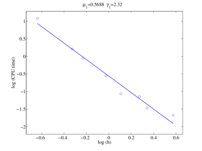
(W)P,asubscriptsubscript𝑊𝑃𝑎\displaystyle(W_{\ell})_{P,a} =μ1Mhγ1,absentsubscript𝜇1subscript𝑀superscriptsubscriptsubscript𝛾1\displaystyle=\mu_{1}M_{\ell}h_{\ell}^{-\gamma_{1}}, (26a)
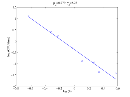
(W)P,ssubscriptsubscript𝑊𝑃𝑠\displaystyle(W_{\ell})_{P,s} =μ2Mhγ2,absentsubscript𝜇2subscript𝑀superscriptsubscriptsubscript𝛾2\displaystyle=\mu_{2}M_{\ell}h_{\ell}^{-\gamma_{2}}, (26b)
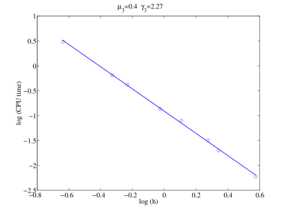
(W)D,asubscriptsubscript𝑊𝐷𝑎\displaystyle(W_{\ell})_{D,a} =μ3Mhγ3,absentsubscript𝜇3subscript𝑀superscriptsubscriptsubscript𝛾3\displaystyle=\mu_{3}M_{\ell}h_{\ell}^{-\gamma_{3}}, (26c)
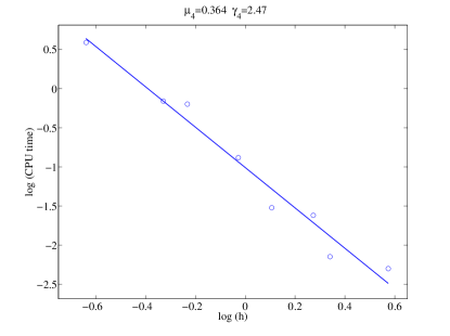
(W)D,ssubscriptsubscript𝑊𝐷𝑠\displaystyle(W_{\ell})_{D,s} =μ4Mhγ4absentsubscript𝜇4subscript𝑀superscriptsubscriptsubscript𝛾4\displaystyle=\mu_{4}M_{\ell}h_{\ell}^{-\gamma_{4}} (26d)

with all μk>0subscript𝜇𝑘0\mu_{k}>0 and γk>0subscript𝛾𝑘0\gamma_{k}>0. Here Msubscript𝑀M_{\ell} is the number of samples used at level \ell, and hsubscripth_{\ell} is the corresponding mesh size.

Analogously, in the case of the vanilla Monte-Carlo method, the computational work is obtained without stratification, i.e., there is only one level. In this case, we will drop the index \ell.

The exponents (and constants) in equations (26) are determined by the algorithm used for assembling the FE matrix in the case of WP,asubscript𝑊𝑃𝑎W_{P,a} and WD,asubscript𝑊𝐷𝑎W_{D,a} (see, e.g., [23] for an efficient algorithm) and by the order of the FE discretization in the case of WP,ssubscript𝑊𝑃𝑠W_{P,s} and WD,ssubscript𝑊𝐷𝑠W_{D,s} (see Section 4.2). The constants μi>0subscript𝜇𝑖0\mu_{i}>0 depend on the implementation.

5.1 The Optimal Monte-Carlo Finite-Element Method

In the case of the Monte-Carlo method, there is only one level so that the index \ell will be dropped. We will choose the optimal M𝑀M and hh such that the total computational cost W𝑊W is minimized given an error bound ϵitalic-ϵ\epsilon to be achieved. This optimization problem with inequality constraints can be solved using the Karush-Kuhn-Tucker (KKT) conditions, which are generalization of Lagrange multipliers in the presence of inequality constraints.

In view of (26) and (16), the most general problem is the following. We minimize the computational work subject to the accuracy constraint RMSEεRMSE𝜀\operatorname{RMSE}\leq\varepsilon, i.e., we solve the optimization problem

minimizeM,h𝑀minimize\displaystyle\underset{M,h}{\text{minimize}} f(M,h):=k=1NμkMhγkassign𝑓𝑀superscriptsubscript𝑘1𝑁subscript𝜇𝑘𝑀superscriptsubscript𝛾𝑘\displaystyle f(M,h):=\sum_{k=1}^{N}\mu_{k}Mh^{-\gamma_{k}} (27)
subject to g1(M,h):=εC0MC1hα0,assignsubscript𝑔1𝑀𝜀subscript𝐶0𝑀subscript𝐶1superscript𝛼0\displaystyle g_{1}(M,h):=\varepsilon-\frac{C_{0}}{\sqrt{M}}-C_{1}h^{\alpha}\geq 0,
g2(M):=M10,assignsubscript𝑔2𝑀𝑀10\displaystyle g_{2}(M):=M-1\geq 0,
g3(h):=hξ0.assignsubscript𝑔3𝜉0\displaystyle g_{3}(h):=h-\xi\geq 0.

Here, N𝑁N\in\mathbb{N} and ξ𝜉\xi is the smallest positive normalized floating-point number representable. Due to the exponents of hh and M𝑀M, it is a nonlinear constraint optimization problem. Our goal is to formulate the inequality constrained problem as an equality constrained problem to which Newton’s method can be applied. In order to solve the optimization problem, we use the interior-point method [24, 25].

For each μ>0𝜇0\mu>0, we replace the non-negativity constraints with logarithmic barrier terms in the objective function

minimizeχ,s𝜒𝑠minimize\displaystyle\underset{\chi,s}{\text{minimize}} fμ(χ,s):=f(χ)μiln(si)assignsubscript𝑓𝜇𝜒𝑠𝑓𝜒𝜇subscript𝑖subscript𝑠𝑖\displaystyle f_{\mu}(\chi,s):=f(\chi)-\mu\sum_{i}\ln(s_{i}) (28)
subject to g(χ)s=0.𝑔𝜒𝑠0\displaystyle g(\chi)-s=0.

Here χ𝜒\chi, a vector, denotes (M,h)𝑀(M,h) and the vectors g𝑔g and s𝑠s represent the gi(x)subscript𝑔𝑖𝑥g_{i}(x) and sisubscript𝑠𝑖s_{i}, respectively. The sisubscript𝑠𝑖s_{i} are restricted to be positive away from zero to ensure that the ln(si)subscript𝑠𝑖\ln(s_{i}) are bounded. As μ𝜇\mu decreases to zero, the minimum of fμsubscript𝑓𝜇f_{\mu} approaches the minimum of f𝑓f. After denoting the Lagrange multiplier for the system (28) by y𝑦y, the system

f(χ)g(χ)Ty𝑓𝜒𝑔superscript𝜒𝑇𝑦\displaystyle\nabla f(\chi)-\nabla g(\chi)^{T}y =0,absent0\displaystyle=0,
SYe𝑆𝑌𝑒\displaystyle SYe =μe,absent𝜇𝑒\displaystyle=\mu e,
g(χ)s𝑔𝜒𝑠\displaystyle g(\chi)-s =0absent0\displaystyle=0

is obtained, where S𝑆S is a diagonal matrix with elements sisubscript𝑠𝑖s_{i}, e𝑒e is a vector of all ones, and g𝑔\nabla g denotes the Jacobian of the constraint g𝑔g. Now we apply Newton’s method to compute the search directions ΔχΔ𝜒\Delta\chi, ΔsΔ𝑠\Delta s, ΔhΔ\Delta h via

(H(χ,y)0A(χ)T0YSA(x)I0)(ΔχΔsΔh)=(f(χ)+A(χ)TyμeSYeg(χ)+s).matrix𝐻𝜒𝑦0𝐴superscript𝜒𝑇0𝑌𝑆𝐴𝑥𝐼0matrixΔ𝜒Δ𝑠Δmatrix𝑓𝜒𝐴superscript𝜒𝑇𝑦𝜇𝑒𝑆𝑌𝑒𝑔𝜒𝑠\begin{pmatrix}H(\chi,y)&0&-A(\chi)^{T}\\ 0&Y&S\\ A(x)&-I&0\end{pmatrix}\begin{pmatrix}\Delta\chi\\ \Delta s\\ \Delta h\end{pmatrix}=\begin{pmatrix}-\nabla f(\chi)+A(\chi)^{T}y\\ \mu e-SYe\\ -g(\chi)+s\end{pmatrix}. (29)

The Hessian matrix is given by

H(χ,y)=2f(χ)iyi2gi(χ)𝐻𝜒𝑦superscript2𝑓𝜒subscript𝑖subscript𝑦𝑖superscript2subscript𝑔𝑖𝜒H(\chi,y)=\nabla^{2}f(\chi)-\sum_{i}y_{i}\nabla^{2}g_{i}(\chi)

and A(χ)𝐴𝜒A(\chi) is the Jacobian matrix of the constraint (27). The second equation is used to calculate ΔsΔ𝑠\Delta s. By substituting into the third equation, we obtain the reduced KKT system

(H(χ,y)A(χ)TA(χ)SY1)(ΔχΔs)=(f(χ)A(χ)Tyh(χ)+μY1e).matrix𝐻𝜒𝑦𝐴superscript𝜒𝑇𝐴𝜒𝑆superscript𝑌1matrixΔ𝜒Δ𝑠matrix𝑓𝜒𝐴superscript𝜒𝑇𝑦𝜒𝜇superscript𝑌1𝑒\begin{pmatrix}-H(\chi,y)&A(\chi)^{T}\\ A(\chi)&SY^{-1}\\ \end{pmatrix}\begin{pmatrix}\Delta\chi\\ \Delta s\\ \end{pmatrix}=\begin{pmatrix}\nabla f(\chi)-A(\chi)^{T}y\\ -h(\chi)+\mu Y^{-1}e\end{pmatrix}. (30)

Now we use iteration to update the solutions by

χ(k+1)superscript𝜒𝑘1\displaystyle\chi^{(k+1)} :=χ(k)+α(k)Δχ(k),assignabsentsuperscript𝜒𝑘superscript𝛼𝑘Δsuperscript𝜒𝑘\displaystyle:=\chi^{(k)}+\alpha^{(k)}\Delta\chi^{(k)},
s(k+1)superscript𝑠𝑘1\displaystyle s^{(k+1)} :=s(k)+α(k)Δs(k),assignabsentsuperscript𝑠𝑘superscript𝛼𝑘Δsuperscript𝑠𝑘\displaystyle:=s^{(k)}+\alpha^{(k)}\Delta s^{(k)},
y(k+1)superscript𝑦𝑘1\displaystyle y^{(k+1)} :=y(k)+α(k)Δy(k),assignabsentsuperscript𝑦𝑘superscript𝛼𝑘Δsuperscript𝑦𝑘\displaystyle:=y^{(k)}+\alpha^{(k)}\Delta y^{(k)},

where (χ(0),s(0),y(0))superscript𝜒0superscript𝑠0superscript𝑦0(\chi^{(0)},s^{(0)},y^{(0)}) is the initial guess and α(k)superscript𝛼𝑘\alpha^{(k)} is chosen to ensure both that s(k+1)>0superscript𝑠𝑘10s^{(k+1)}>0 and the objective function

Ψυ,μ(χ,s)=fμ(χ,s)+υ2g(χ)s,subscriptΨ𝜐𝜇𝜒𝑠subscript𝑓𝜇𝜒𝑠𝜐2norm𝑔𝜒𝑠\Psi_{\upsilon,\mu}(\chi,s)=f_{\mu}(\chi,s)+\frac{\upsilon}{2}\|g(\chi)-s\|,

is sufficiently reduced [26]. The parameter υ𝜐\upsilon may increase with the iteration number to force the solution toward feasibility.

5.2 The Optimal Multi-Level Monte-Carlo Finite-Element Method

For an optimal multi-level Monte-Carlo finite-element method, our goal is to determine the optimal hierarchies (L,{M}=0L,h0,r)𝐿superscriptsubscriptsubscript𝑀0𝐿subscript0𝑟(L,\left\{M_{\ell}\right\}_{\ell=0}^{L},h_{0},r) which minimize the computational work subject to the given accuracy constraint RMSEεRMSE𝜀\operatorname{RMSE}\leq\varepsilon. The optimal number L𝐿L of levels is also unknown a priori. To this end, we solve the optimization problem

minimizeM,h0,rsubscript𝑀subscript0𝑟minimize\displaystyle\underset{M_{\ell},h_{0},r}{\text{minimize}} f(M,h0,r,L):==0Lk=1NμkMh0γkrγkassign𝑓subscript𝑀subscript0𝑟𝐿superscriptsubscript0𝐿superscriptsubscript𝑘1𝑁subscript𝜇𝑘subscript𝑀superscriptsubscript0subscript𝛾𝑘superscript𝑟subscript𝛾𝑘\displaystyle f(M_{\ell},h_{0},r,L):=\sum_{\ell=0}^{L}\sum_{k=1}^{N}\mu_{k}M_{\ell}h_{0}^{-\gamma_{k}}r^{\ell\gamma_{k}} (31)
subject to g1(M,h0,r,L):=εC00M0C0=1L1Mh0βr(1)βC1h0αrLα0,assignsubscript𝑔1subscript𝑀subscript0𝑟𝐿𝜀subscript𝐶00subscript𝑀0subscript𝐶0superscriptsubscript1𝐿1subscript𝑀superscriptsubscript0𝛽superscript𝑟1𝛽subscript𝐶1superscriptsubscript0𝛼superscript𝑟𝐿𝛼0\displaystyle g_{1}(M_{\ell},h_{0},r,L):=\varepsilon-\frac{C_{00}}{\sqrt{M_{0}}}-C_{0}\sum_{\ell=1}^{L}\frac{1}{\sqrt{M}_{\ell}}h_{0}^{\beta}r^{-(\ell-1)\beta}-C_{1}h_{0}^{\alpha}r^{-L\alpha}\geq 0,
g2(M):=M10,=0,,L,formulae-sequenceassignsubscript𝑔2subscript𝑀subscript𝑀100𝐿\displaystyle g_{2}(M_{\ell}):=M_{\ell}-1\geq 0,\qquad\ell=0,\ldots,L,
g3(h0):=h0ξ0,assignsubscript𝑔3subscript0subscript0𝜉0\displaystyle g_{3}(h_{0}):=h_{0}-\xi\geq 0,
g4(r):=r10,assignsubscript𝑔4𝑟𝑟10\displaystyle g_{4}(r):=r-1\geq 0,

where N𝑁N\in\mathbb{N} and ξ𝜉\xi is the smallest positive normalized floating-point number representable by the machine.

Similar to the vanilla Monte-Carlo case, we use the interior-point method to solve this nonlinear problem and optimize the hierarchies. In problems with two or three physical/spatial dimensions, the optimal determination of the mesh sizes hsubscripth_{\ell} is a crucial factor in the optimization problem specifically if the exponents γksubscript𝛾𝑘\gamma_{k} are greater than 111.

There are two options: one is to choose the hsubscripth_{\ell} as a geometric progression according to (8). In this case, we solve the minimization problem (31). The other is to choose the mesh sizes hsubscripth_{\ell} freely such that they only satisfy the natural condition

h0h1h2hL.subscript0subscript1subscript2subscript𝐿h_{0}\geq h_{1}\geq h_{2}\geq\cdots\geq h_{L}.

We will explore both options in Section 6.

In the second case, when the mesh sizes are freely chosen, we write them as

h:=h0r,=1,,L,formulae-sequenceassignsubscriptsubscript0subscript𝑟1𝐿h_{\ell}:=\frac{h_{0}}{r_{\ell}},\qquad\ell=1,\ldots,L,

where r:=i=1riassignsubscript𝑟superscriptsubscriptproduct𝑖1subscript𝑟𝑖r_{\ell}:=\prod_{i=1}^{\ell}r_{i} with ri1subscript𝑟𝑖1r_{i}\geq 1. It is clear that rLrL1r11subscript𝑟𝐿subscript𝑟𝐿1subscript𝑟11r_{L}\geq r_{L-1}\ldots\geq r_{1}\geq 1. Hence, in (31), we may replace r𝑟r by rsubscript𝑟r_{\ell} and then the optimization problem can be rewritten as

minimizeM,h0,rsubscript𝑀subscript0subscript𝑟minimize\displaystyle\underset{M_{\ell},h_{0},r_{\ell}}{\text{minimize}} f(M,h0,r,L):==0Lk=1NμkMh0γkrγkassign𝑓subscript𝑀subscript0subscript𝑟𝐿superscriptsubscript0𝐿superscriptsubscript𝑘1𝑁subscript𝜇𝑘subscript𝑀superscriptsubscript0subscript𝛾𝑘superscriptsubscript𝑟subscript𝛾𝑘\displaystyle f(M_{\ell},h_{0},r_{\ell},L):=\sum_{\ell=0}^{L}\sum_{k=1}^{N}\mu_{k}M_{\ell}h_{0}^{-\gamma_{k}}r_{\ell}^{\gamma_{k}} (32)
subject to g1(M,h0,r,L):=εC00M0C0=1L1Mh0βr1βC1h0αrLα0,assignsubscript𝑔1subscript𝑀subscript0subscript𝑟𝐿𝜀subscript𝐶00subscript𝑀0subscript𝐶0superscriptsubscript1𝐿1subscript𝑀superscriptsubscript0𝛽superscriptsubscript𝑟1𝛽subscript𝐶1superscriptsubscript0𝛼superscriptsubscript𝑟𝐿𝛼0\displaystyle g_{1}(M_{\ell},h_{0},r_{\ell},L):=\varepsilon-\frac{C_{00}}{\sqrt{M_{0}}}-C_{0}\sum_{\ell=1}^{L}\frac{1}{\sqrt{M}_{\ell}}h_{0}^{\beta}r_{\ell-1}^{-\beta}-C_{1}h_{0}^{\alpha}r_{L}^{-\alpha}\geq 0,
g2(M):=M10,=0,,L,formulae-sequenceassignsubscript𝑔2subscript𝑀subscript𝑀100𝐿\displaystyle g_{2}(M_{\ell}):=M_{\ell}-1\geq 0,\qquad\ell=0,\ldots,L,
g3(h0):=h0ξ0,assignsubscript𝑔3subscript0subscript0𝜉0\displaystyle g_{3}(h_{0}):=h_{0}-\xi\geq 0,
g4:=ri10,1iand=1,,L.formulae-sequenceassignsubscript𝑔4subscript𝑟𝑖101𝑖and1𝐿\displaystyle g_{4}:=r_{i}-1\geq 0,\quad 1\leq i\leq\ell\quad\text{and}\quad\ell=1,\ldots,L.

In the next section, we apply these two approaches to a MLMC FE method and discuss their efficiency.

6 Numerical Results

In this section, we present numerical results for the Monte-Carlo and multi-level Monte-Carlo methods for the drift-diffusion-Poisson system. We also investigate the choices of the FE mesh sizes on each level, namely as geometric progressions or freely chosen. The random coefficients in the drift-diffusion-Poisson system considered here stem from a real-world application, namely the effect of random dopants in nanoscale semiconductor devices, which is of great importance in its own right.

6.1 The Leading Example

Random-dopant effects are called discrete-dopant fluctuation effects [27, 28, 29]. In nanoscale semiconductor devices, the charge profile of the dopant atoms cannot be validly modeled as a continuum anymore, but the random location of each dopant needs to be taken into account. This means that each device is a realization of a random process and corresponds to an event ω𝜔\omega. In this manner, the potential and carrier-density fluctuations due to the discreteness and randomness of the dopants are clearly captured.

Here the silicon lattice is doped with boron as the impurity atoms. The domain D2𝐷superscript2D\subset\mathbb{R}^{2} is depicted in Figure 2. The thickness of the oxide layer is 8nm8nm8\,\mathrm{nm}, the thickness of the nanowire is 50nm50nm50\,\mathrm{nm}, and its width is 60nm60nm60\,\mathrm{nm}. Regarding the geometry, Dirichlet boundary conditions are used at the contacts with a back-gate voltage of 1V1V-1\,\mathrm{V} (at the bottom of the device) and an electrode voltage of 0V0V0\,\mathrm{V} (at the top of the device). Zero Neumann boundary conditions are used everywhere else. The relative permittivities in the subdomains are ASi=11.7subscript𝐴Si11.7A_{\mathrm{Si}}=11.7, Aox=3.9subscript𝐴ox3.9A_{\mathrm{ox}}=3.9, Aliq=78subscript𝐴liq78A_{\mathrm{liq}}=78, and Adop=4.2subscript𝐴dop4.2A_{\mathrm{dop}}=4.2. The number of dopants placed randomly in the device corresponds to a doping concentration of 1016cm3superscript1016superscriptcm310^{16}\,\mathrm{cm^{-3}}. According to its volume, the silicon subdomain hence contains 666 negative impurity atoms when Cdop=51015cm3subscript𝐶dop5superscript1015superscriptcm3C_{\mathrm{dop}}=5\cdot 10^{15}\,\mathrm{cm^{-3}} and 600600600 dopants when Cdop=51017cm3subscript𝐶dop5superscript1017superscriptcm3C_{\mathrm{dop}}=5\cdot 10^{17}\,\mathrm{cm^{-3}}.

In order to solve the system of equations, we use Scharfetter-Gummel iteration. In spite of the quadratic convergence of Newton’s method for the system, Scharfetter-Gummel iteration has advantages for the problem at hand. First of all, Scharfetter-Gummel iteration is much less sensitive to the choice of the initial guess than Newton’s method. Another important feature is the reduced computational effort and memory requirement, since in each iteration it requires the successive solution of three much smaller elliptic problems.
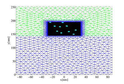
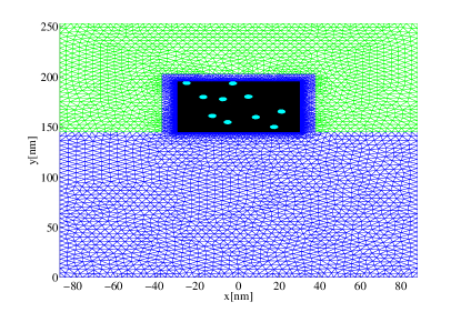
Refer to caption
(a)
Refer to caption
(b)
Figure 2: Meshes for the random distribution of impurity atoms (cyan circles) in a nanowire field-effect sensor for levels =00\ell=0 (left) and =11\ell=1 (right), where h0=5subscript05h_{0}=5, r=2𝑟2r=2, and Cdop=21017cm3subscript𝐶dop2superscript1017superscriptcm3C_{\mathrm{dop}}=2\cdot 10^{17}\,\mathrm{cm^{-3}}. Additionally, oxide subdomain (Doxsubscript𝐷oxD_{\text{ox}}), trandsucer (DSisubscript𝐷SiD_{\text{Si}}) and the electrolyte (Dliqsubscript𝐷liqD_{\text{liq}}) are depicted with blue, balck and green meshes respectively.
Refer to caption
(a)
Refer to caption
(b)
Refer to caption
(c)
Refer to caption
(d)
Figure 3: Computational work for matrix assembly (top) and solving the system (bottom), both for the Poisson equation (left) and the drift-diffusion-equations (right).

6.2 The Computational Work

As the first step, we calculate the coefficients in the expressions (26) for the computational work. To that end, we solve the system for various mesh sizes and measure the time spent on matrix assembly and solving the resulting system, both for the Poisson equation and the drift-diffusion equations. Figure 3 shows the results for the coefficients in the expressions for the computational work.

The coefficients α𝛼\alpha and C1subscript𝐶1C_{1} in the FE discretization error

𝔼[VV^h]X+𝔼[uu^h]X+𝔼[vv^h]XC1hαsubscriptnorm𝔼delimited-[]𝑉subscript^𝑉𝑋subscriptnorm𝔼delimited-[]𝑢subscript^𝑢𝑋subscriptnorm𝔼delimited-[]𝑣subscript^𝑣𝑋subscript𝐶1superscript𝛼\|\mathbb{E}[V-\hat{V}_{h}]\|_{X}+\|\mathbb{E}[u-\hat{u}_{h}]\|_{X}+\|\mathbb{E}[v-\hat{v}_{h}]\|_{X}\leq C_{1}h^{\alpha}

of the system are given in Figure 4. The exponent α=0.96𝛼0.96\alpha=0.96 found here agrees very well with the order of the discretization used here, i.e., P1subscript𝑃1P_{1} finite elements.

For the statistical error, we determine the coefficients in the inequality

(σ[ΔVh0]+σ[ΔVh])+(σ[Δuh0]+σ[Δuh])+(σ[Δvh0]+σ[Δvh])C00+C0h1β.𝜎delimited-[]Δsubscript𝑉subscript0𝜎delimited-[]Δsubscript𝑉subscript𝜎delimited-[]Δsubscript𝑢subscript0𝜎delimited-[]Δsubscript𝑢subscript𝜎delimited-[]Δsubscript𝑣subscript0𝜎delimited-[]Δsubscript𝑣subscriptsubscript𝐶00subscript𝐶0superscriptsubscript1𝛽(\sigma[\Delta V_{h_{0}}]+\sigma[\Delta V_{h_{\ell}}])+(\sigma[\Delta u_{h_{0}}]+\sigma[\Delta u_{h_{\ell}}])+(\sigma[\Delta v_{h_{0}}]+\sigma[\Delta v_{h_{\ell}}])\leq C_{00}+C_{0}h_{\ell-1}^{\beta}.

Here C00=0.197subscript𝐶000.197C_{00}=0.197 and the rest of the coefficients are shown in Figure 4.
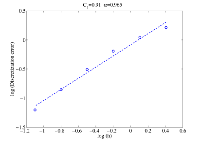
Refer to caption
(a)
Refer to caption
(b)
Figure 4: Discretization error (left) and statistical (right) error as a function of hh.

6.3 Optimization

Having determined the coefficients in the expressions for the computational work, it is now possible to numerically solve the optimization problems. As described in Section 5, we apply an iterative interior-point method to optimize both the number of samples and mesh sizes. The results here are obtained for ξ=252𝜉superscript252\xi=2^{-52}.

6.3.1 Monte Carlo

First of all, we solve the optimization problem (27) for the MC-FE method. Because there is only one level, it is straightforward to solve. The optimal values for the MC FE method are summarized in Table 1 for given ε𝜀\varepsilon.

ε𝜀\varepsilon 0.1 0.05 0.03 0.02 0.01 0.005 0.002
hh 0.054 0.026 0.015 0.010 0.005 0.002 0.001
M𝑀M 19 77 214 483 1940 7785 48 845
Table 1: Optimal MC FE method parameters for various given error tolerances.

6.3.2 Multi-Level Monte Carlo

In the MLMC-FE method, determining the optimal number of levels is an important part of the calculation. This is achieved here by solving the optimization problem for several levels starting with a single level and noting that the computational work increases above a certain number of levels. More precisely, we solve the optimization problem (31) for 0L80𝐿80\leq L\leq 8 levels as well as for various given error bounds.

Since the number of samples in each level is a continuous variable in the optimization problem, the optimal number of levels is – in general – not an integer and hence we choose Msubscript𝑀\lfloor M_{\ell}\rfloor, =0,,L0𝐿\ell=0,\ldots,L, as the final numbers of levels. Therefore, due to the second constraint g2subscript𝑔2g_{2}, Msubscript𝑀M_{\ell} is an integer greater equal 111 for all levels.

Refer to caption
(a)
Refer to caption
(b)
Figure 5: The minimized computational work for the MLMC-FE method as a function of the number of levels and as a function of the given error tolerance. The results for a geometric progression for hh (left) and general hh (right) are shown. The number of levels yielding the minimal overall computational work is indicated by red circles.
Refer to caption
Figure 6: Comparison between the two different approaches to MLMC FE method for ε=0.03𝜀0.03\varepsilon=0.03.

The results of the optimization problems provide insight into the MLMC procedure. Figure 5 shows the minimized computational work as a function of the number of levels and as a function of the given tolerance. It shows that for smaller tolerances, more levels are necessary to obtain the smallest computational work.

In Figure 6, the two approaches to multi-level Monte Carlo are compared, namely choosing the hsubscripth_{\ell} as a geometric progressions or freely. Due to generality of the second option, the total work when choosing the hsubscripth_{\ell} freely is lower compared to the first option. The results for both approaches to MLMC-FEM are summarized in Tables 2 and 3 for various given error tolerances.

ε𝜀\varepsilon h0subscript0h_{0} r𝑟r M0subscript𝑀0M_{0} M1subscript𝑀1M_{1} M2subscript𝑀2M_{2} M3subscript𝑀3M_{3} M4subscript𝑀4M_{4} M5subscript𝑀5M_{5} M6subscript𝑀6M_{6}
0.10.10.1 0.359 2.650 59 4 1
0.050.050.05 0.350 2.430 276 22 2 1
0.030.030.03 0.329 2.830 779 46 2 1
0.020.020.02 0.339 2.440 1 993 152 12 1 1
0.010.010.01 0.347 2.355 9 428 786 69 6 1 1
0.0050.0050.005 0.332 2.670 39 142 2 526 154 9 1 1
0.0020.0020.002 0.334 2.647 286 181 18 986 1200 76 6 1 1
Table 2: Optimal levels for the MLMC-FE method with hsubscripth_{\ell} chosen as a geometric progression for given error tolerances ε𝜀\varepsilon.
ε𝜀\varepsilon h0subscript0h_{0} r1subscript𝑟1r_{1} r2subscript𝑟2r_{2} r3subscript𝑟3r_{3} r4subscript𝑟4r_{4} r5subscript𝑟5r_{5} r6subscript𝑟6r_{6}
0.10.10.1 0.366 2.100 3.490
0.050.050.05 0.360 2.168 1.860 3.712
0.030.030.03 0.343 2.351 2.138 4.750
0.020.020.02 0.346 2.317 2.086 1.744 4.348
0.010.010.01 0.339 2.400 2.218 1.938 1.536 4.554
0.0050.0050.005 0.332 2.483 2.348 2.134 1.812 6.220
0.0020.0020.002 0.328 2.541 2.442 2.280 2.030 1.670 7.142
ε𝜀\varepsilon M0subscript𝑀0M_{0} M1subscript𝑀1M_{1} M2subscript𝑀2M_{2} M3subscript𝑀3M_{3} M4subscript𝑀4M_{4} M5subscript𝑀5M_{5} M6subscript𝑀6M_{6}
0.10.10.1 59 6 1
0.050.050.05 280 28 4 1
0.030.030.03 800 66 7 1
0.020.020.02 2 012 171 19 3 1
0.010.010.01 8 897 697 66 8 2 1
0.0050.0050.005 38 251 2 778 229 24 4 1
0.0020.0020.002 271 031 18 667 1408 124 14 3 1
Table 3: Optimal levels for the MLMC-FE method with general hsubscripth_{\ell} for given error tolerances ε𝜀\varepsilon.

6.3.3 Comparison

Finally, as Figure 7 shows, the computational work for the multi-level Monte-Carlo method is approximately 10 times lower than the one for the Monte-Carlo method for larger tolerance levels such as ε=0.1𝜀0.1\varepsilon=0.1. The effectiveness of the MLMC-FE method is more pronounced for smaller error bounds; for ε=0.005𝜀0.005\varepsilon=0.005, the computational work is about a factor 104superscript10410^{4} lower than the Monte-Carlo work.

The optimal distribution of the samples among the levels in the multi-level method leads to more evaluations in the first levels (which are cheaper) and to fewer evaluations in the higher levels. On the other hand, to satisfy the first constraint of (27), the Monte-Carlo method needs a smaller mesh size compared to the multi-level method, which greatly increases the total computational work although the total number of samples is lower.
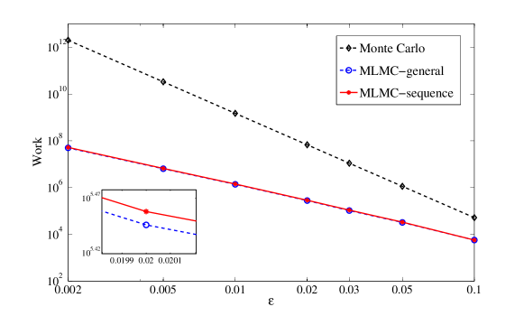
Refer to caption
Figure 7: Comparison of total computational work for MC-FEM and the two approaches to MLMC-FEM for various given tolerances.

7 Conclusions

In this work, we considered the stochastic drift-diffusion-Poisson equations as the main model equation for describing transport in random environments with many applications. We presented existence and local uniqueness theorems for the weak solution of the system. We also developed MC- and MLMC-FE methods for this system of stochastic PDEs.

Additionally, we balanced the various parameters in the numerical methods by viewing this problem as a global optimization problem. The goal is to determine the numerical parameters such that the computational work to achieve a total error, i.e., discretization error plus statistical error, less than or equal to a given error tolerance is minimized.

Although the exponential terms in the constraints make the optimization problems nonlinear, the optimization problems can be solved by an interior-point method with sufficient iterations. The solution of the constrained optimization problem leads to optimal (M𝑀M, hh) in the case of the vanilla MC method and to hierarchies consisting of (L,{M}=0L,h0,r)𝐿superscriptsubscriptsubscript𝑀0𝐿subscript0𝑟(L,\left\{M_{\ell}\right\}_{\ell=0}^{L},h_{0},r) in the case of the MLMC method.

Moreover, we investigated two different options to the mesh refinement in the multi-level method. In the comparison of the MC with the MLMC method, the MLMC method was found to decrease the total computational effort by four orders of magnitude for small error tolerances. The speed-up becomes better as the error tolerance decreases.

8 Acknowledgments

The authors acknowledge support by FWF (Austrian Science Fund) START project no. Y660 PDE Models for Nanotechnology. The authors acknowledge discussions with Dr. Masoud Ahookhosh (University of Luxembourg) about numerical optimization methods.

References

  • [1] C. Heitzinger, N. J. Mauser, C. Ringhofer, Multiscale modeling of planar and nanowire field-effect biosensors, SIAM Journal on Applied Mathematics 70 (5) (2010) 1634–1654.
  • [2] S. Baumgartner, C. Heitzinger, Existence and local uniqueness for 3D self-consistent multiscale models for field-effect sensors, Commun. Math. Sci 10 (2) (2012) 693–716.
  • [3] S. Baumgartner, C. Heitzinger, A one-level FETI method for the drift-diffusion-Poisson system with discontinuities at an interface, J. Comput. Phys. 243 (2013) 74–86. doi:10.1016/j.jcp.2013.02.043.
    URL http://dx.doi.org/10.1016/j.jcp.2013.02.043
  • [4] S. Baumgartner, C. Heitzinger, A. Vacic, M. A. Reed, Predictive simulations and optimization of nanowire field-effect PSA sensors including screening, Nanotechnology 24 (22) (2013) 225503/1–9. doi:10.1088/0957-4484/24/22/225503.
    URL http://stacks.iop.org/0957-4484/24/225503
  • [5] C. Heitzinger, C. Ringhofer, Multiscale modeling of fluctuations in stochastic elliptic PDE models of nanosensors, Commun. Math. Sci. 12 (3) (2014) 401–421. doi:10.4310/CMS.2014.v12.n3.a1.
    URL http://dx.doi.org/10.4310/CMS.2014.v12.n3.a1
  • [6] G. Tulzer, C. Heitzinger, Fluctuations due to association and dissociation processes at nanowire-biosensor surfaces and their optimal design, Nanotechnology 26 (2) (2015) 025502.
  • [7] C. Heitzinger, Y. Liu, N. J. Mauser, C. Ringhofer, R. W. Dutton, Calculation of fluctuations in boundary layers of nanowire field-effect biosensors, Journal of Computational and Theoretical Nanoscience 7 (12) (2010) 2574–2580.
  • [8] M. B. Giles, Multilevel Monte Carlo path simulation, Operations Research 56 (3) (2008) 607–617.
  • [9] S. Heinrich, Multilevel Monte Carlo methods, in: Large-scale scientific computing, Springer, 2001, pp. 58–67.
  • [10] M. Giles, Improved multilevel Monte Carlo convergence using the Milstein scheme, in: Monte Carlo and quasi-Monte Carlo methods 2006, Springer, 2008, pp. 343–358.
  • [11] M. B. Giles, B. J. Waterhouse, Multilevel quasi-Monte Carlo path simulation, Advanced Financial Modelling, Radon Series on Computational and Applied Mathematics (2009) 165–181.
  • [12] A. Barth, C. Schwab, N. Zollinger, Multi-level Monte Carlo finite element method for elliptic PDEs with stochastic coefficients, Numerische Mathematik 119 (1) (2011) 123–161.
  • [13] A. Cliffe, M. Giles, R. Scheichl, A. Teckentrup, Multilevel Monte Carlo methods and applications to elliptic PDEs with random coefficients, Computing and Visualization in Science 14 (1) (2011) 3–15.
  • [14] F. Y. Kuo, C. Schwab, I. H. Sloan, Quasi-Monte Carlo finite element methods for a class of elliptic partial differential equations with random coefficients, SIAM Journal on Numerical Analysis 50 (6) (2012) 3351–3374.
  • [15] J. Charrier, R. Scheichl, A. Teckentrup, Finite element error analysis of elliptic PDEs with random coefficients and its application to multilevel Monte Carlo methods, SIAM Journal on Numerical Analysis 51 (1) (2013) 322–352.
  • [16] A. Teckentrup, R. Scheichl, M. Giles, E. Ullmann, Further analysis of multilevel Monte Carlo methods for elliptic PDEs with random coefficients, Numerische Mathematik 125 (3) (2013) 569–600.
  • [17] A.-L. Haji-Ali, F. Nobile, E. von Schwerin, R. Tempone, Optimization of mesh hierarchies in multilevel Monte Carlo samplers, Stochastic Partial Differential Equations: Analysis and Computations (2015) 1–37.
  • [18] P. A. Markowich, C. Ringhofer, C. Schmeiser., Semiconductor Equations, Springer, Wien, 1990.
  • [19] A. Bulyha, C. Heitzinger, An algorithm for three-dimensional Monte-Carlo simulation of charge distribution at biofunctionalized surfaces, Nanoscale 3 (4) (2011) 1608–1617.
  • [20] A. Fort, S. Rocchi, M. B. Serrano-Santos, R. Spinicci, V. Vignoli, Surface state model for conductance responses during thermal-modulation of SnO-based thick film sensors: Part I—model derivation, IEEE Transactions on Instrumentation and Measurement 55 (6) (2006) 2102–2106.
  • [21] G. Tulzer, S. Baumgartner, E. Brunet, G. C. Mutinati, S. Steinhauer, A. Köck, P. E. Barbano, C. Heitzinger, Kinetic parameter estimation and fluctuation analysis of CO at SnO2 single nanowires, Nanotechnology 24 (31) (2013) 315501/1–10. doi:10.1088/0957-4484/24/31/315501.
    URL http://iopscience.iop.org/0957-4484/24/31/315501/
  • [22] C. Heitzinger, L. Taghizadeh, Existence and local uniqueness for the Stokes-Nernst-Planck-Drift-Diffusion-Poisson system modeling nanowire sensors and nanopores, In preparation.
  • [23] F. Cuvelier, C. Japhet, G. Scarella, An efficient way to perform the assembly of finite element matrices in Matlab and Octave, Tech. Rep. 8305, Université Paris 13 and INRIA Paris-Rocquencourt (May 2013).
  • [24] A. Forsgren, P. E. Gill, M. H. Wright, Interior methods for nonlinear optimization, SIAM review 44 (4) (2002) 525–597.
  • [25] M. Wright, The interior-point revolution in optimization: history, recent developments, and lasting consequences, Bulletin of the American Mathematical Society 42 (1) (2005) 39–56.
  • [26] H. Y. Benson, D. F. Shanno, R. J. Vanderbei, Interior-point methods for nonconvex nonlinear programming: Jamming and comparative numerical testing, Operations Research and Financial Engineering, Princeton University, ORFE-00-02.
  • [27] B. Van Zeghbroeck, Principles of semiconductor devices, Colarado University.
  • [28] S. Roy, A. Asenov, Where do the dopants go?, Science 309 (5733) (2005) 388–390.
  • [29] A. Khodadadian, C. Heitzinger, Basis adaptation for the stochastic Poisson-Boltzmann equation, Submitted to Journal of Computational electronics.