An enhanced finite element method for a class of variational problems exhibiting the Lavrentiev gap phenomenon

Abstract

This paper develops an enhanced finite element method for approximating a class of variational problems which exhibit the Lavrentiev gap phenomenon in the sense that the minimum values of the energy functional have a nontrivial gap when the functional is minimized on spaces $W^{1,1}$ and $W^{1,\infty}$. To remedy the standard finite element method, which fails to converge for such variational problems, a simple and effective cut-off procedure is utilized to design the (enhanced finite element) discrete energy functional. In essence the proposed discrete energy functional curbs the gap phenomenon by capping the derivatives of its input on a scale of $O(h^{-\alpha})$ (where $h$ denotes the mesh size) for some positive constant $\alpha$. A sufficient condition is proposed for determining the problem-dependent parameter $\alpha$. Extensive 1-D and 2-D numerical experiment results are provided to show the convergence behavior and the performance of the proposed enhanced finite element method.

1 Introduction

This paper concerns with finite element approximations of variational problems whose solutions (or minimizers) exhibit the so-called Lavrentiev gap phenomenon - a defect from the singularities of the solutions. Such problems are often encountered in materials sciences, nonlinear elasticity, and image processing (cf. [7, 13, 4] and the references therein). These variational problems can be abstractly stated as follows:

(1) $$u=\operatorname*{argmin}_{v\in\mathcal{A}}\mathcal{J}(v),$$

where the energy functional $\mathcal{J}:\mathcal{A}\to\mathbb{R}\cup\{\pm\infty\}$ is defined by

(2) $$\mathcal{J}(v)=\int_{\Omega}f(\nabla v,v,x)\operatorname{d}\!{x}.$$

Where $\Omega\subset\mathbb{R}^{n}$ is an open and bounded domain, $f:\mathbb{R}^{n}\times\mathbb{R}\times\Omega\to\mathbb{R}$, called the density function of $\mathcal{J}$, is assumed to be a continuous function, The space $\mathcal{A}:=\{v\in W^{1,1}(\Omega):v=g\text{ on }\partial\Omega\}$ is known as the admissible set, $g\in L^{1}(\partial\Omega)$ is some given function.

Let $\mathcal{A}_{\infty}:=\mathcal{A}\cap W^{1,\infty}(\Omega)$. Since $\Omega$ is bounded, then $\mathcal{A}\subset\mathcal{A}_{\infty}$ and consequently there holds

(3) $$\inf_{v\in\mathcal{A}_{1}}\mathcal{J}(v)\leq\inf_{v\in\mathcal{A}_{\infty}}\mathcal{J}(v).$$

Problem (1) is said to exhibit the Lavrentiev gap phenomenon whenever

(4) $$\inf_{v\in\mathcal{A}_{1}}\mathcal{J}(v)<\inf_{v\in\mathcal{A}_{\infty}}\mathcal{J}(v),$$

in other words, when the strict inequality holds in (3).

The gap between the minimum values on both sides of (4) suggests that the the minimizer of the left-hand side must have some singularity which causes the gap. Such a singularity often corresponds to a defect in a material or an edge in an image. It has been known in the literature [7, 13, 4] that the gap phenomenon could happen not only for nonconvex energy functionals but also for strictly convex and coercive energy functionals. As a result, it is a very complicated phenomenon to characterize and to analyze as well as to approximate (see below for details), because the gap phenomenon can be triggered by quite different mechanisms and the definition of the Lavrentiev gap phenomenon is a very broad concept which covers many different types of singularities. To the best of our knowledge, so far there is no known general sufficient conditions which guarantee the existence of the gap phenomenon.

The simplest and best known example of the gap phenomenon is Maniá’s 1-D problem [11], where one minimizes the functional

(5) $$\mathcal{J}(v)=\int_{0}^{1}v^{\prime}(x)^{6}\bigl{(}v(x)^{3}-x\bigr{)}^{2}\operatorname{d}\!{x}$$

over all functions $v\in W^{1,1}(0,1)$ satisfying $v(0)=0$ and $v(1)=1$. By inspection it is easy to see that $u(x)=x^{\frac{1}{3}}$ minimizes (5) with a minimum value zero. However, it can be shown that the minimum over space $W^{1,\infty}(0,1)$ (i.e., the space of all Lipschitz functions) is strictly larger than zero. As a result, Maniá’s problem does exhibits the Lavrentiev gap phenomenon. Notice that $u^{\prime}(x)=\frac{1}{3}x^{-\frac{2}{3}}$ which blows up rapidly as $x\to 0^{+}$. Moreover, a more striking property, which was proved by Ball and Knowles (cf. [2]), is that if $u_{j}$ is a sequence of functions in $W^{1,q}(0,1)$ for $q\geq\frac{3}{2}$ with $u_{j}(0)=0$ and $u_{j}(1)=1$ such that $u_{j}\to u$ a.e. as $j\to\infty$, then $\mathcal{J}(u_{j})\to\infty$ as $j\to\infty$. Since the finite element space $V^{h}_{r}$ (see section 2 for its definition) is a subspace of $W^{1,\infty}$, the above properties of the functional $\mathcal{J}$ imply that the standard finite element approximations to Maniá’s problem must fail to approximate both the minimizer and the minimum value of the functional. Such a conclusion was indeed verified numerically in [7, 13], also see Figure 1 for another numerical verification. This negative result immediately leads to the following two conclusions: first, variational problems which exhibit the gap phenomenon are difficult and delicate to approximate numerically; second, nonstandard numerical methods must be designed for such problems in order to correctly approximate both the minimizers and the minimum values. The failure of the standard finite element method suggests that in order to ensure the convergence of any numerical method which uses $V^{h}_{r}$ as the approximation space, one needs to construct a discrete energy functional $\mathcal{J}_{h}$ which necessarily does not coincide with $\mathcal{J}$ on the finite element space $V^{h}_{r}$.

As expected, there have been a few successful attempts to design convergent numerical methods for variational problems with the gap phenomenon. Below we only focus on discussing the methods which use conforming finite element methods to approximate variational problems with the Maniá-type gap phenomenon, by which we mean that the minimizers of the variational problems blow up in the $W^{1,\infty}$-norm. but it is important to note that some gap phenomenon problems have been solved with the use of penalty and nonconforming finite element methods [4, 3, 12].

The first numerical method was proposed by Ball and Knowles in [2]. To handle the difficulty caused by the rapid blow-up in $W^{1,\infty}$-norm of the minimizer $u$, they proposed to approximate $u$ and its derivative $u^{\prime}$ simultaneously, an idea which is often seen in mixed finite element methods. Specifically, the authors proposed to minimize the discrete energy functional

(6) $$\mathcal{J}_{h}^{BK}(v_{h},w_{h})=\int_{\Omega}f(w_{h},v_{h},x)\operatorname{d}\!{x}$$

under the constraint

$$\|\phi(v_{h}^{\prime}-w_{h})\|_{L^{1}(\Omega)}\leq\varepsilon_{h}$$

for some super-linear function $\phi$ over all functions $(v_{h},w_{h})\in V^{h}_{1}\times V^{h}_{0}$, where $V^{h}_{0}$ and $V^{h}_{1}$ denote respectively the discontinuous piecewise constant space and the continuous piecewise affine finite element space associated with a mesh $\mathcal{T}_{h}$ of $\Omega$. Where $\{\varepsilon_{h}\}$ is a sequence such that $\varepsilon_{h}\to 0$ as $h\to 0$. Notice that $\mathcal{J}_{h}^{BK}$ essentially has the same form as the original functional $\mathcal{J}$ after setting $w_{h}=v_{h}^{\prime}$. While this method works and is well-posed on the discrete level, the decoupling of $v_{h}$ and $v_{h}^{\prime}$ adds an additional layer of unknowns which increases the complexity of the discrete minimization problem. Moreover, its generalization to higher dimensions is not straightforward. The other major numerical developments were carried out by Z. Li et al. in [9, 8, 1]. Their work has brought two similar methods: an element removal method and a truncation method. Here we only detail the truncation method and briefly mention the element removal method because the latter is similar to the former and the truncation method is more closely related to our method to be introduced in this paper. Let $s\geq 1$ and $M_{h}>0$. Define the discrete energy functional

(7) $$\mathcal{J}_{h}^{Li}(v_{h})=\sum_{T\in\mathcal{T}_{h}}\mathcal{J}_{h}^{Li}(v_{h};T)$$

where

$$\mathcal{J}_{h}^{Li}(v_{h};T) =\min\left\{\mathcal{J}_{h}(v_{h};T),\,M_{h}\left(1+\|\nabla v_{h}\|_{L^{s}(T)}\right)\right\},$$

$$\mathcal{J}_{h}(v_{h};T) =\int_{T}f(\nabla v_{h},v_{h},x)\operatorname{d}\!{x}.$$

Here the truncation substitutes the contribution of $\mathcal{J}_{h}(v_{h},T)$ by another constant if $v_{h}$ behaves “poorly” on $T$. The element removal method simply discards (i.e., sets $\mathcal{J}_{h}^{Li}(v_{h},T)=0$ on) those “bad” elements. Both methods are robust and calculate the minimum value of $\mathcal{J}$ over $\mathcal{A}_{\infty}$ (assuming the minimizer $u$ uniquely exists). However, the determination of $M_{h}$ and $s$ (or “bad” elements) requires a litany of a priori assumptions, some of which depend on the sought-after exact minimizer $u$.

The goal of this paper is to introduce an effective and robust numerical method which slightly alters the standard finite element method by a novel and simple cut-off procedure. Our approach is motivated by the rationale that the standard finite element method fails to work because the magnitude of the gradient $\nabla u_{h}$ becomes too large (independent of the magnitude of $u_{h}$, where $u_{h}$ stands for the standard finite element solution) near the singularity points. So the idea of our cut-off procedure is simply to limit the growth of $|\nabla u_{h}|$ to $\mathcal{O}(h^{-\alpha})$ order in the whole domain $\Omega$, the resulting discrete energy functional is then given by

(8) $$\mathcal{J}_{h}^{\alpha}(w_{h})=\int_{\Omega}f\bigl{(}\chi_{h}^{\alpha}(\nabla w_{h}),w_{h},x\bigr{)}\,dx,$$

where $\chi_{h}^{\alpha}(\cdot)$ denotes the cut-off function (see section 3 for its definition). It is important to note that, unlike the truncation method of [1], the choice of the crucial parameter $\alpha$ does not depend on any a priori knowledge about the exact minimizer $u$, instead, it only depends on the structure of the energy density function $f$ and the space $\mathcal{A}$. Moreover, we shall provide a sufficient condition, which is easy to use, for determining an upper bound for $\alpha$ to ensure the convergence.

The organization of the paper is as follows. In section 2 we introduce the notation, preliminary results such as finite element meshes and spaces. In section 3 we state the variational problems we aim to solve and the assumptions under which we develop our numerical method. We then define our finite element method with a help of the above cut-off procedure. We also present the alluded sufficient condition for determining an upper bound for $\alpha$ and demonstrate its utility using Maniá’s problem. In section 4 we provide some extensive numerical experiment results for two specific application problems to gauge the performance of the proposed enhanced finite element method. Finally, the paper is ended with some concluding remarks in section 5.

2 Preliminaries

Standard function and space notation will be adopted throughout this paper. For example, for an open and bounded domain $\Omega\subset\mathbb{R}^{n}$ with boundary $\partial\Omega$, let $W^{1,p}(\Omega)$ for $1\leq p\leq\infty$ denotes the Sobolev space consisting of functions whose up to first order weak derivatives are $L^{\infty}$-integrable over $\Omega$ and $\|\cdot\|_{W^{1,p}(\Omega)}$ denotes the standard norm on $W^{1,p}(\Omega)$. $\mathcal{A}$ and $\mathcal{A}_{\infty}$ have been introduced in section 1, we also define the space $\mathcal{A}_{p}:=\mathcal{A}\cap W^{1,p}(\Omega)$ for any $p\in(1,\infty)$.

Let $f$ and $\mathcal{J}$ be the same as in (2) and the variational problem to be considered in the rest of this paper is given by (1). Suppose that problem (1) has a unique solution $u$ which exhibits the Lavrentiev gap phenomenon as defined in section 1, that is, we assume there holds inequality

(9) $$\inf_{v\in\mathcal{A}_{1}}\mathcal{J}(v)<\inf_{v\in\mathcal{A}_{\infty}}\mathcal{J}(v).$$

So our primary goal is to construct an effective and robust finite element method to approximate $u$.

To this end, let $\mathcal{T}_{h}$ be a quasi-uniform triangular (when $n=2$) or tetrahedral (when $n=3$) mesh of $\Omega$ with mesh parameter $h>0$. For a positive integer $r$, we define the finite element space $V^{h}_{r}$ on $\mathcal{T}_{h}$ by

(10) $$V^{h}_{r}:=\bigl{\{}v_{h}\in\mathcal{A}\cap C^{0}(\overline{\Omega}):\,{v_{h}}|_{T}\in\mathbb{P}_{r}(T)\quad\forall T\in\mathcal{T}_{h}\bigr{\}},$$

where $\mathbb{P}_{r}(T)$ denotes the set of all polynomials whose degrees do not exceed $r$.

It is easy to see that $V^{h}_{r}\subset\mathcal{A}_{\infty}\subset\mathcal{A}$ for all $h>0$, then an obvious attempt to formulate a numerical method for variational problem (1) is the following standard finite element method which seeks $u_{h}\in V^{h}_{r}$ such that

(11) $$u_{h}=\operatorname*{argmin}_{v_{h}\in V^{h}_{r}}\mathcal{J}(v_{h}).$$

Unfortunately, this finite element method fails to give a convergent method because the method cannot give the true minimum value if (9) holds and will not converge to the correct minimizer as the numerical test shows in Figure 1.

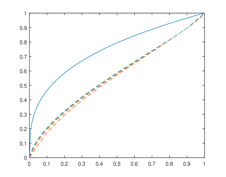
Fig. 1: The standard finite element method applied to Maniá’s problem (5). The solid line is the true solution $u(x)=x^{\frac{1}{3}}$ and the dashed lines are the finite element minimizers $u_{h}$ for $h=\frac{1}{N}$ where $N=10,20,40,80,160$. All minimizations were implemented by using the MATLAB minimization routine fminunc with initial function $u_{0}(x)=x$.

To see the deeper reason, we note that for any $v\in\mathcal{A}$ with $\mathcal{J}(v)<\infty$, the existence of a sequence of functions $\hat{v}_{h}\in V_{h}$ with $\hat{v}_{h}\to v$ in $\mathcal{A}$ such that

(12) $$\lim_{h\to 0}\mathcal{J}_{h}(\hat{v}_{h})=\mathcal{J}(v)$$

is a key step to show convergence of the discrete minimizers. It is clear that (9) implies that

$$\mathcal{J}(\hat{u}_{h})\geq\inf_{v\in\mathcal{A}_{\infty}}\mathcal{J}(v)>\mathcal{J}(u)$$

for any $\hat{u}_{h}\in V^{h}_{r}$ with $\hat{u}_{h}\to u$ in $\mathcal{A}$, which contradicts with (12) for the minimizer $u$. In fact, it was proved by C. Ortner in [12] that for a class of convex energies the convergence (to the exact solution) of the standard finite element method is equivalent to (9) not holding (i.e., the gap phenomenon does not occur).

3 Formulation of the enhanced finite element method

From the analysis given in the previous section we conclude that in order to construct a convergent numerical method which uses $V^{h}_{r}$ as an approximation space, we must design a discrete energy functional $\mathcal{J}_{h}$ which should not coincide with $\mathcal{J}$ on the finite element space $V^{h}_{r}$. In this section we shall construct a discrete energy functional $\mathcal{J}_{h}$ which meets this criterion and provides a convergent (nonstandard) finite element method for problem (1).

Before introducing our method, let us give a heuristic discussion about why the gap phenomenon is appearing and how the existing methods assuage its effect. Consider Maniá’s problem (5). For any $v_{h}\in V_{h}$ (or in $\mathcal{A}_{\infty}$) sufficiently approximating $u(x)=x^{\frac{1}{3}}$, the quantity $(v_{h}^{3}-x)^{2}$ will be small but always nonzero. However, at the same time $|v_{h}^{\prime}|$ will be very large near the origin. If $|v_{h}^{\prime}|$ is raised to a high enough power - six in this case - then the error of $(v_{h}^{3}-x)^{2}$ will be magnified to be so large that the quantity

$$\int_{0}^{h}(v_{h}^{\prime})^{6}(v_{h}^{3}-x)^{2}\operatorname{d}\!{x}$$

will not vanish as $h\to 0$. For this reason, all of the existing methods were designed to dampen the effect of the derivative in the integral. The method of Ball and Knowles [2] weakly enforces $v_{h}^{\prime}=w_{h}$ which allows the method to soften the effect of $v_{h}^{\prime}$, where $v_{h}^{\prime}$ has a singularity, and achieves convergence. The methods of Li et al. [1] leave the function $f$ unchanged, but remove or replace the functional value on the elements where something has gone wrong.

With this in mind we now introduce a discrete energy functional which is much simpler and has a majority of the characteristics of the methods in [9, 8, 1]. Our approach is motivated by the belief that the standard finite element method fails to work because the magnitude of the gradient $\nabla u_{h}$ becomes too large (independent of the magnitude of $u_{h}$, where $u_{h}$ denotes the solution to (11)) near the singularity points. So our idea is simply to use a cut-off procedure to limit the growth of $|\nabla u_{h}|$ to $\mathcal{O}(h^{-\alpha})$ on the whole domain $\Omega$ in our discrete energy functional $\mathcal{J}_{h}$. To this end, let $\alpha>0$, define the cut-off function $\chi_{h}^{\alpha}:\mathbb{R}^{n}\to\mathbb{R}^{n}$ in the $i$th component by

(13) $$\left[\chi_{h}^{\alpha}(s)\right]_{i}=\begin{cases}s_{i}&\text{ if }|s_{i}|\leq h^{-\alpha}\\ \mbox{sign}(s_{i})h^{-\alpha}&\text{ if }|s_{i}|>h^{-\alpha}\end{cases},\qquad i=1,2,\ldots n.$$

It is clear that this function merely cuts the value of $s_{i}$ to a constant $\operatorname*{sgn}(s_{i})h^{-\alpha}$ if $|s_{i}|$ is too large. Then our discrete functional is simply defined as

(14) $$\mathcal{J}_{h}^{\alpha}(v_{h})=\int_{\Omega}f\bigl{(}\chi_{h}^{\alpha}(\nabla v_{h}),v_{h},x\bigr{)}\operatorname{d}\!{x},$$

and our enhanced finite element method is defined by seeking $u_{h}\in V^{h}_{r}$ such that

(15) $$u_{h}=\operatorname*{argmin}_{v_{h}\in V^{h}_{r}}\mathcal{J}_{h}^{\alpha}(v_{h}).$$

Remark 3.1.

Since our discrete energy functional $\mathcal{J}_{h}^{\alpha}$ curbs the gap phenomenon by capping the derivative of its input on a scale of $\mathcal{O}(h^{-\alpha})$, spiritually it is similar to the truncation method of Li et al. [1], but unlike the truncation method it keeps the dynamics of $f$ with respect to $v$ and $x$ much like Ball and Knowles’ approach in [2]. Implementing the cut-off procedure is very simple and can be done by adding a few lines of code. Moreover, unlike the truncation method, our enhanced finite element method does not require a priori knowledge about the exact minimizer $u$ of (1). Further adding to the simplicity is the existence of only one parameter $\alpha$ in the method. Here $\alpha$ controls the rate at which the cut-off grows and is the key for the convergence of the method. In general, $\alpha$ needs to be chosen in order to obtain equation (12) for all $v\in\mathcal{A}$ where $I_{h}v\in V^{h}_{r}$ is the finite element interpolant of $v$. Indeed, (12) is the only restriction we impose upon $\alpha$. A permissible range for $\alpha$, which guarantees convergence, depends on the structure of the density function $f$, so it is problem-dependent. Below we use Maniá’s problem to demonstrate the process.

We now derive an upper bound for $\alpha$ such that (12) holds for $v\in\mathcal{A}$. For a fixed $v\in\mathcal{A}$, notice that $\mathcal{J}(v)<\infty$, let $I_{h}v\in V^{h}_{r}$ denote the finite element interpolant of $v$. We want to find an uppper bound for $\alpha$ such that $\mathcal{J}_{h}^{\alpha}(I_{h}v)\to\mathcal{J}(v)$ as $h\to 0$ because this will guarantee (12) for $v$. Let $\delta>0$. Adding and subtracting $v$, using Young’s inequality with weight $h^{\delta}$, and using the definition of $\chi_{h}^{\alpha}$ we get

$$\mathcal{J}_{h}^{\alpha}(v_{h})=\int_{0}^{1}(\chi_{h}^{\alpha}(v_{h}^{\prime}))^{6}(v_{h}^{3}-x)^{2}\operatorname{d}\!{x}$$

$$\quad=\int_{0}^{1}(\chi_{h}^{\alpha}(v_{h}^{\prime}))^{6}(v_{h}^{3}-v^{3}+v^{3}-x)^{2}\operatorname{d}\!{x}$$

$$\quad\leq\int_{0}^{1}(1+h^{-\delta})(\chi_{h}^{\alpha}(v_{h}^{\prime}))^{6}(v_{h}^{3}-v^{3})^{2}\operatorname{d}\!{x}+\int_{0}^{1}(1+h^{\delta})(\chi_{h}^{\alpha}(v_{h}^{\prime}))^{6}(v^{3}-x)^{2}\operatorname{d}\!{x}$$

$$\quad\leq\int_{0}^{1}(1+h^{-\delta})h^{-6\alpha}(v_{h}^{3}-v^{3})^{2}\operatorname{d}\!{x}+\int_{0}^{1}(1+h^{\delta})(v_{h}^{\prime})^{6}(v^{3}-x)^{2}\operatorname{d}\!{x}$$

$$\quad=:A_{1}^{h}+A_{2}^{h}.$$

Since $v^{3}-x$ factor now has no error, multiplying by $(v^{\prime}_{h})^{6}$ does not have a magnification effect which is the source of the gap phenomenon, it can be shown that [5] $A_{2}^{h}\to\mathcal{J}(v)$ as $h\to 0$, then we have (12) provided $A_{1}^{h}$ vanishes. We claim that $A_{1}^{h}$ vanishes as $h\to 0$ for $0<\alpha<\frac{1}{6}$. The proof of the assertion goes as follows. By Hölder’s Inequality we have

$$A_{1}^{h} =(1+h^{-\delta})h^{-6\alpha}\int_{0}^{1}(v_{h}^{3}-v^{3})^{2}\operatorname{d}\!{x}$$

$$=(1+h^{-\delta})h^{-6\alpha}\int_{0}^{1}(v_{h}-v)^{2}(v_{h}^{2}+v_{h}v+v^{2})^{2}\operatorname{d}\!{x}$$

$$\leq(1+h^{-\delta})h^{-6\alpha}\|v_{h}-v\|_{L^{2}(\Omega)}^{2}\|(v_{h}^{2}+v_{h}v+v^{2})^{2}\|_{L^{\infty}(\Omega)}.$$

Since $v_{h}=I_{h}v$ we have that $v_{h}$ is uniformly bounded in $h$ and $\|v_{h}-v\|_{L^{2}(\Omega)}^{2}=\mathcal{O}(h)$. Thus

$$0\leq A_{1}^{h}\leq\|(v_{h}^{2}+v_{h}v+v^{2})^{2}\|_{L^{\infty}(\Omega)}(1+h^{-\delta})h^{1-6\alpha}$$

Since $\alpha<\frac{1}{6}$ we may choose $\delta<1-6\alpha$ such that $A_{1}^{h}\to 0$ as $h\to 0$ and we have (12). Clearly, this range of $\alpha$ does not depend on the solution $u$ but only on the form of $f$ and the regularity of the space $\mathcal{A}$. We regard this property as one crucial advantage of our method.

4 Numerical experiments

In this section we present some numerical experiment results for two variational problems which are known to exhibit the gap phenomenon. The first problem is Maniá’s 1-D problem which has been seen in the previous sections; the second problem, which was proposed by Foss in [6], is a 2-D variational problem from nonlinear elasticity. For each of the two test problems we solve it by using our enhanced finite element method with linear element (i.e., $r=1$), and we solve the minimization problem (15) by using the MATLAB minimization function fminunc. We first demonstrate the convergence of the numerical method, we then numerically evaluate the effect and sharpness of the parameter $\alpha$, and compare with the standard finite element method (which is known to be divergent). We also numerically compute the rate of convergence for $u-u_{h}$ although no theoretical rate convergence has yet been proved for the numerical method.

4.1 Maniá’s 1-D problem

Once again, the energy functional of Maniá’s 1-D problem is given by (5). A uniform mesh $\mathcal{T}_{h}$ with mesh size $h$ and the linear finite element are used in the test. As mentioned above, we solve the resulting minimization problem (15) by using the MATLAB minimization function fminunc with initial function $u_{0}(x)=x$.

Figure 2 displays the computed solutions (minimizers) $u_{h}$ with various mesh size $h$ along with the exact solution $u(x)=x^{\frac{1}{3}}$. The parameter $\alpha=\frac{1}{4}$ is used for the tests. It is clear that the solutions $u_{h}$ are correctly approximating $u$. Figure 3 shows the behavior of the absolute value of the error function $u-u_{h}$. As expected, we see that the location where the biggest error occurs moves closer to the singularity point $x=0$ of $u$ as the mesh size $h$ gets smaller.

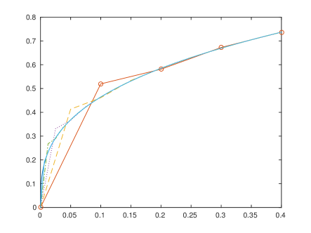
Fig. 2: The graphs of the computed minimizers/solution $u_{h}$ of the enhanced FEM applied to Maniá’s problem (5) with parameter $\alpha=\frac{1}{4}$ from $x=0$ to $x=0.4$. The solid line is the exact solution $u(x)=x^{\frac{1}{3}}$ and the dashed and circled lines are the minimizers $u_{h}$ for $h=\frac{1}{N}$ where $N=10,20,40,80,160$. All minimizations were implemented by using the MATLAB minimization function fminunc with initial function $u_{0}(x)=x$.

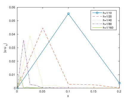
Fig. 3: The graphs of the errors $|u_{h}-u|$ of the enhanced FEM applied to Maniá’s problem (5) with parameter $\alpha=\frac{1}{4}$ from $x=0$ to $x=0.2$ for $h=\frac{1}{N}$ where $N=10,20,40,80,160$. All minimizations were implemented by using the MATLAB minimization function fminunc with initial function $u_{0}(x)=x$.

For a more detailed look, we also record the $L^{\infty}$-norms of the error $u-u_{h}$ and compute the rate of convergence in Table 1. Clearly, the table shows the convergence of the computed solutions $u_{h}$. As a comparison and to see that these approximations would not be found using the standard finite element method, a comparison of the values of $\mathcal{J}$ and $\mathcal{J}_{h}^{\alpha}$ at $u_{h}$, $I^{1}_{h}u$, and $I_{h}^{2}(u)$ is given in Table 2, where $I_{h}^{1}$ and $I_{h}^{2}$ are the piecewise linear and quadratic interpolants respectively. We see here that $\mathcal{J}_{h}^{\alpha}$ correctly captures the dynamics needed to obtain a convergent sequence of solutions $u_{h}$ while the sequences $\{\mathcal{J}(u_{h})\}$ and $\{\mathcal{J}(I_{h}u)\}$ do not. In addition $\{\mathcal{J}_{h}^{\alpha}(I_{h}^{1}u)\}$ and $\{\mathcal{J}_{h}^{\alpha}(I_{h}^{2}u)\}$ converge with the same rate, $\mathcal{O}(h^{1.5})$. Thus employing higher order elements on this problem will not result in a larger convergence rate. To make this clear we plot the convergence rate of the numerical minimizers $u_{h}$ of $\mathcal{J}_{h}^{\alpha}$ for linear and quadratic elements in Figure 4. Note both elements observe the same convergence rate of 1.5.

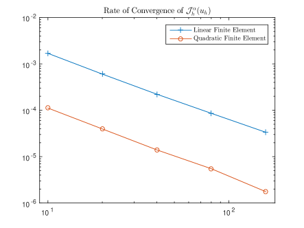
Fig. 4: The rate of convergence of $\mathcal{J}_{h}^{\alpha}(u_{h})$ where $u_{h}$ is the solution to enhanced FEM applied to Maniá’s problem (5) with parameter $\alpha=\frac{1}{4}$ for $h=\frac{1}{N}$ where $N=10,20,40,80,160$. Plotted are the rates for the linear and quadratic finite element spaces. All minimizations were implemented by using the MATLAB minimization function fminunc with initial function $u_{0}(x)=x^{1/2}$.

$h$	1/10	1/20	1/40	1/80	1/160
$\|u-u_{h}\|_{L^{\infty}}$	5.53e-2	4.50e-2	3.88e-2	3.59e-2	8.32e-3
rate	-	0.30	0.20	0.11	2.10

Table 1: The $L^{\infty}$ errors between $u$ and $u_{h}$ where $u_{h}$ are the solutions of the enhanced FEM applied to Maniá’s problem (5) with parameter $\alpha=\frac{1}{4}$.

$h$	1/10	1/20	1/40	1/80	1/160
$\mathcal{J}(u_{h})$	8.23e-1	1.64	3.28	6.56	13.1
$\mathcal{J}_{h}^{\alpha}(u_{h})$	1.68e-3	6.02e-4	2.22e-5	8.59e-6	3.31e-5
$\mathcal{J}(I_{h}^{1}u)$	7.19e-1	1.52	3.04	6.09	12.9
$\mathcal{J}_{h}^{\alpha}(I_{h}^{1}u)$	2.41e-3	8.63e-4	3.09e-4	1.10e-4	3.91e-5
$\mathcal{J}(I_{h}^{2}u)$	1.16	2.31	4.62	9.24	18.5
$\mathcal{J}_{h}^{\alpha}(I_{h}^{2}u)$	1.71e-4	6.03e-5	3.09e-4	7.54e-6	2.67e-6

Table 2: The functional values $\mathcal{J}$ and $\mathcal{J}_{h}^{\alpha}$ for $u_{h}$, $I_{h}^{1}u$, and $I_{h}^{2}u$, where $u_{h}$ are the solutions of the enhanced FEM applied to Maniá’s problem (5) with parameter $\alpha=\frac{1}{4}$, and $I_{h}^{1}u$ and $I_{h}^{2}u$ is the piecewise linear and quadratic nodal interpolant of the exact solution/minimizer $u$.

Finally, we examine the role of the parameter $\alpha$. In section 3 we show that $\alpha<\frac{1}{2}$ is sufficient to ensure (9) for all $v\in\mathcal{A}$ with finite energy. Our numerical tests show that for any $\alpha<1/2$ the enhanced finite element method converges for Maniá’s problem, and the convergence of $|\mathcal{J}_{h}^{\alpha}(u_{h})-\mathcal{J}(u)|\to 0$ diminishes as $\alpha\to\frac{1}{2}$. So $\alpha^{*}:=\frac{1}{2}$ seems a critical point for the choice of $\alpha$ for linear, quadratic, and higher order nodal finite elements. It must be noted that taking $\alpha$ close to $\alpha^{*}$ is not a good idea. Notice that the Euler-Lagrange equation of (5) is a nonlinear equation. To solve the nonlinear equation, a mesh restriction $h<h^{\prime}$ is expected and it takes up the most of the total CPU time for solving the nonlinear equation. This mesh restriction is expected to depend on $\alpha$. To see this, let

$$\tilde{u}_{h}=\operatorname*{argmin}_{v_{h}\in V_{h}}\mathcal{J}(u_{h})$$

be the solution to the standard finite element method. Suppose that $\alpha$ is close to $\frac{1}{2}$, we observe that $\mathcal{J}_{h}^{\alpha}(\tilde{u}_{h})\approx\mathcal{J}(\tilde{u}_{h})$. While $\mathcal{J}_{h}^{\alpha}(I_{h}u)$ indeed converges to $\mathcal{J}(u)$ the convergence is very slow. Since the upper bound $h^{\prime}$ must be chosen such that for all $h<h^{\prime}$ we have

$$\mathcal{J}_{h}^{\alpha}(I_{h}u)<\mathcal{J}_{h}^{\alpha}(\tilde{u}_{h}),$$

so $h^{\prime}$ must be extremely small and approaches $0$ as $\alpha\to\frac{1}{2}$. On noting the fact that for all $h\geq h^{\prime}$ a small perturbation of $\tilde{u}_{h}$ will be a minimizer of $\mathcal{J}_{h}^{\alpha}$ over $V_{h}$, we see that $\alpha$ must be chosen carefully in order to guarantee that we can obtain good numerical solutions with any mesh sizes $h<h^{\prime}$. To show this important detail graphically, Figure 5 displays the computed solutions/minimizers $u_{h}$ to $\mathcal{J}_{h}^{\alpha}$ with $\alpha=\frac{2}{7}$. We observe that for $h=\frac{1}{10}$ and $h=\frac{1}{20}$, $u_{h}$ do not approximate $u$ well, but for $h=\frac{1}{40}$, $h=\frac{1}{180}$ and $h=\frac{1}{160}$, $u_{h}$ gives much more accurate approximations.

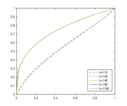
Fig. 5: The graphs of the computed solutions/minimizers $u_{h}$ of the enhanced FEM applied to the Maniá’s problem (5) with parameter $\alpha=\frac{2}{7}$ for $h=\frac{1}{N}$ where $N=10,20,40,80,160$. The dotted lines are for $N=10$ and $20$ while the solid lines are for $N=40,80,$ and $160$. All minimizations were implemented by using the MATLAB minimization function fminunc with initial function $u_{0}(x)=x$.

4.2 Foss’ 2-D problem

We now consider a 2-D variational problem which exhibits the Lavrentiev gap phenomenon. It arises from nonlinear elasticity and was first studied by M. Foss in [6], and its numerical approximation was investigated by Li et al. in [1].

Let $\Omega=(0,1)\times(\frac{3}{2},\frac{5}{2})$, the energy functional of Foss’ problem is given by

(16) $$\mathcal{J}(v)=66\Bigl{(}\frac{13}{14}\Bigr{)}^{14}\int_{\Omega}\Bigl{(}\frac{y}{y-1}\Bigr{)}^{14}|u|^{\frac{14-3y}{y-1}}\bigl{(}|u|^{\frac{y}{y-1}}-x\bigr{)}^{2}(u_{x})^{14}\operatorname{d}\!{x}\operatorname{d}\!{y},$$

and the admissible set is $\mathcal{A}=\{u\in W^{1,1}(\Omega):u(0,\cdot)=0\text{ and }u(1,\cdot)=1\}$. It was shown by Foss [6] that

$$0=\inf_{v\in\mathcal{A}}\mathcal{J}(v)<\inf_{v\in\mathcal{A}_{\infty}}\mathcal{J}(v)=1,$$

which proves that $\mathcal{J}$ does exhibit the gap phenomenon. Moreover, the minimizer of $\mathcal{J}$ over $\mathcal{A}$ is given by $u(x,y)=x^{\frac{y-1}{y}}$, but the problem does not attain its minimum value in $\mathcal{A}_{\infty}$.

We apply our enhanced finite element method with $\alpha=\frac{1}{6}$ to solve Foss’ problem. In order to generate a reasonably good initial guess for using the MATLAB minimization function fminunc, we first compute

(17) $$\tilde{u}_{h}=\operatorname*{argmin}_{v_{h}\in V_{h}}\mathcal{J}(v_{h})$$

using the MATLAB routine fminunc with initial guess $u(x,y)=x$ and then use $\tilde{u}_{h}$ as an initial condition for solving

(18) $$u_{h}=\operatorname*{argmin}_{v_{h}\in V_{h}}\mathcal{J}_{h}^{\alpha}(v_{h})$$

using the same MATLAB routine fminunc.

Figure 6 presents the error plots of both $|\hat{u}_{h}-u|$ and $|u_{h}-u|$ over the domain $\Omega$. We observe that $|\tilde{u}_{h}-u|$ does not converge to zero while $|u_{h}-u|$ does. In addition, Table 3 shows that the cut-off procedure is sufficient in order to guarantee convergence for (16). Using the same reasoning as to show (12) for Maniá’s problem, a value of $\alpha<\frac{3}{14}$ is sufficient for the proposed enhanced finite element method to work. However, computing the functional values $\mathcal{J}_{h}^{\alpha}(I_{h}u)$ with different values of $\alpha$ shows that $\alpha=\frac{1}{2}$ and $\alpha=\frac{10}{17}$ also result in convergent methods.

$h$	1/6	1/12	1/24
$\mathcal{J}(\tilde{u}_{h})$	14.84	5.71	3.21
$\mathcal{J}_{h}^{\alpha}(\tilde{u}_{h})$	11.46	4.74	2.68
$\mathcal{J}(u_{h})$	3330	3914	4047
$\mathcal{J}_{h}^{\alpha}(u_{h})$	1.28e-1	5.45e-3	5.28e-4

Table 3: The functional values $\mathcal{J}$ and $\mathcal{J}_{h}^{\alpha}$ at $\tilde{u}_{h}$ and $u_{h}$, where $\tilde{u}_{h}$ and $u_{h}$ satisfy (17) and (18) respectively for problem (16). Here $\alpha=\frac{1}{6}$.

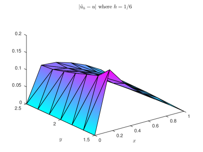
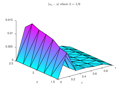
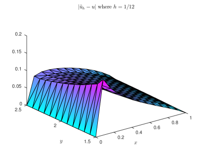
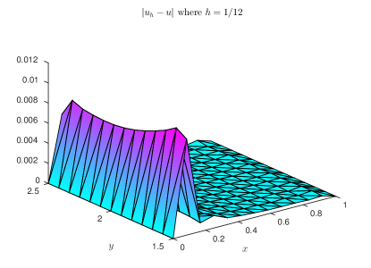
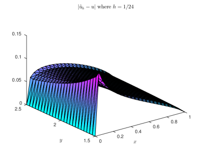
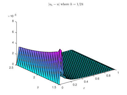
Fig. 6: The graphs of the error function $|u-\tilde{u}_{h}|$ (left column) and the error function $|u-u_{h}|$ (right column) with $\alpha=\frac{1}{6}$ for $h=\frac{1}{6},\frac{1}{12}$, and $\frac{1}{24}$. All minimizations were done by using the MATLAB minimization function fminunc.

5 Conclusion

In this paper we proposed an enhanced finite element method for variational problems that exhibits the Lavrentiev gap phenomenon. The method uses the Lagrange finite element spaces and a discrete energy functional that is constructed by using a novel cut-off procedure. It is simple to construct and easy to implemented simply by adding a few extra lines of code. Unlike some existing numerical methods, the formulation of the proposed enhanced finite element method does not depend on a priori knowledge about the exact solutions/minimizers. Only one problem-dependent parameter needs to be chosen in order to use the method. A sufficient and easy-to-use condition was provided for its determination. We presented extensive numerical experiment results for two benchmark problems for the Lavrentiev gap phenomenon, namely, Maniá’s 1-D problem and Foss’ 2-D problem. Our numerical results show that the proposed enhanced finite element method works very well, it is effective, robust and convergent.

It is clear that the crux of the proposed enhanced finite element method is the cut-off procedure, it caps the growth of $\nabla v_{h}$ to the order of $O(h^{-\alpha})$ in the whole domain. Clearly, this procedure is independent of the underlying finite element method, consequently, it is natural and temptable to substitute the finite element space $V^{h}_{r}$ in the formulation by other approximation spaces, such as nonconforming finite element spaces and discontinuous Galerkin (DG) spaces. After taking care a few details which are well-known when transitioning from the finite element method to DG and nonconforming methods, this generalization indeed can be easily done. In fact, although we only presented the formulation and numerical experiments in the context of the finite element method, we have also numerically tested DG methods with and without the cut-off procedure, the outcome is exactly same as for the finite element method, that is, the standard DG method does not give a convergent method, but the enhanced DG method (with the cut-off procedure) does. Further details on various generalizations of the work presented in this paper will be reported in a forthcoming paper.

Besides the generalizations of using approximation spaces other than finite element spaces, there are a few important and interesting issues which need to be addressed. The foremost issue perhaps is to provide a qualitative convergence analysis for the proposed enhanced finite element method. Such a project has already been undertaken using the $\Gamma$-convergence approach and will be reported later in [5]. Since the singularities of the minimizers are often isolated, it is expected and also verified by our numerical experiments that the biggest errors are occurred near the singularity points, and very fine meshes are required to resolve these singularities. To improve efficiency and to reduce the computational cost, It is natural to incorporate unstructured meshes and adaptive algorithms, which only use very fine meshes near the singularity points, into the enhanced finite element method. In this regard, the cut-off procedure provides an immediate a posteriori indicator for mesh refinement, that is, the mesh is only refined where the cut-off function is triggered. Such an idea is worthy of further investigation and will be reported in another forthcoming work.

References

- [1] Y. Bai and Z.-P. Li. A truncation method for detecting singular minimizers involving the Lavrentiev phenomenon. Math. Models Methods Appl. Sci., 16(6):847–867, 2006.
- [2] J. M. Ball and G. Knowles. A numerical method for detecting singular minimizers. Numer. Math., 51(2):181–197, 1987.
- [3] C. Carstensen and C. Ortner. Analysis of a class of penalty methods for computing singular minimizers. Comput. Methods Appl. Math., 10(2):137-163, 2010.
- [4] C. Carstensen and C. Ortner. Computation of the Lavrentiev phenomenon. OxMoS Preprint, No. 17, 2009.
- [5] X. Feng and S. Schnake. -convergence of an enhanced finite element method for approximating singular minimizers. in preparation.
- [6] M. Foss. Examples of the Lavrentiev phenomenon with continuous Sobolev exponent dependence. J. Convex Anal., 10(2):445–464, 2003.
- [7] M. Foss, W. J. Hrusa, and V. J. Mizel. The Lavrentiev gap phenomenon in nonlinear elasticity. Arch. Ration. Mech. Anal., 167(4):337–365, 2003.
- [8] Z.-P. Li. A numerical method for computing singular minimizers. Numer. Math., 71:317–330, 1995.
- [9] Z.-P. Li. Element removal method for singular minimizers in variational problems involving Lavrentiev phenomenon. Proc. Roy. Soc. London Ser. A, 439(1905):131–137, 1992.
- [10] M. Lavrentiev. Sur quelques problemes du calcul des variations.. Ann. Mat. Pura e App., 4:7–28, 1926.
- [11] B. Maniá. Soppa un esempio di lavrentieff. Ball. Unione Mat. Ital, 13:147–153, 1934.
- [12] C. Ortner. Nonconforming finite-element discretization of convex variational problems. IMA J. Numer. Anal., 31(3):847–864, 2011.
- [13] M. Winter. Lavrentiev phenomenon in microstructure theory. Electron. J. Diff. Eqns., 6:1–12, 1996.