Constraining quantum collapse inflationary models with CMB data

Abstract

The hypothesis of the self-induced collapse of the inflaton wave function was proposed as responsible for the emergence of inhomogeneity and anisotropy at all scales. This proposal was studied within an almost de Sitter space-time approximation for the background, which led to a perfect scale-invariant power spectrum, and also for a quasi-de Sitter background, which allows to distinguish departures from the standard approach due to the inclusion of the collapse hypothesis. In this work we perform a Bayesian model comparison for two different choices of the self-induced collapse in a full quasi-de Sitter expansion scenario. In particular, we analyze the possibility of detecting the imprint of these collapse schemes at low multipoles of the anisotropy temperature power spectrum of the Cosmic Microwave Background (CMB) using the most recent data provided by the Planck Collaboration. Our results show that one of the two collapse schemes analyzed provides the same Bayesian evidence of the minimal standard cosmological model $\Lambda$CDM, while the other scenario is weakly disfavoured with respect to the standard cosmology.

I Introduction

According to the standard inflationary paradigm, the origin of the cosmic structures is explained by a background Friedmann-Robertson-Walker (FRW) cosmology with a nearly exponential expansion driven by the potential of a single scalar field and from its quantum fluctuations characterised by a simple vacuum state. However, when this picture is considered more carefully, a conceptual issue arises: while the initial state that characterises the quantum perturbations of both the inflaton field and the metric is highly homogeneous and isotropic, the present state of the universe is described by a state with inhomogeneities and anisotropies. As known, the quantum unitary evolution can not be responsible for breaking the initial symmetries of the early quantum state. This issue has been discussed in previous papers Perez et al. (2005); Sudarsky (2011); de Unánue and Sudarsky (2008); León and Sudarsky (2010); Diez-Tejedor and Sudarsky (2012); León et al. (2011); Landau et al. (2012, 2013); León et al. (2015a); Cañate et al. (2013), where the collapse proposal has been developed. The key ingredient of this proposal is to assume a self-induced collapse of the inflaton wave function as the responsible for the emergence of inhomogeneities and anistropies at each particular length scale.

The idea that the collapse of the wave function could be regarded as an actual physical process induced by gravity was proposed in Refs. Penrose (1996); Diosi (1987, 1989); Ghirardi et al. (1986). On the other hand, various proposals of that sort have been developed for studying problems in different context than the cosmological one Ghirardi et al. (1986); Pearle (1989); Bassi and Ghirardi (2003); Bassi et al. (2013). These proposals might well be compatible with the self-induced collapse of the inflaton’s wave function that we are considering. Here, the hypothesis simply assumes that something intrinsic to the system, i.e., independent of external agents (e.g., observers), triggers the collapse or reduction of the quantum mechanical state of the system. The proposal is, at this point, a purely phenomenological scheme. It does not attempt to describe the process in terms of some specific new physical theory, but just to provide a general parameterisation of the quantum transition involved. It is worth mentioning that the previous conceptual problem is sometimes known in the literature as the quantum-to-classical transition of the primordial perturbations. In this context, some authors have argued that decoherence Kiefer and Polarski (2008); Grishchuk and Sidorov (1990) can give a good explanation of the emergence of anisotropies and inhomogeneities. Other approaches seem to adopt the Everett “many-worlds” interpretation of quantum mechanics when confronted with this problem. However, it has been shown that neither decoherence Adler (2001); Schlosshauer (2004) nor the Everettian formulation can solve the quantum measurement problem (we refer the reader to Perez et al. (2005); Sudarsky (2011); León and Sudarsky (2010); León et al. (2011); Landau et al. (2013) for a detailed discussion of this issue).

In order to treat the collapse process, we assume that at a certain stage in cosmic evolution there is an induced jump in a state describing a particular mode of the quantum field, in a such similar way of a quantum mechanical collapse of the wave function associated with a measurement. However in our scheme there is no external measuring device or observer responsible for triggering such collapse. The next issue is to define the characteristic of the state in which such jump occurs. In particular, we need a criterion to determine the expectation values of the field and the momentum conjugate variables for the post-collapse state, without relying on some particular collapse mechanism. In previous works, Perez et al. (2005); de Unánue and Sudarsky (2008); León et al. (2011, 2015a) various possibilities regarding the description of the quantum expectation values in the post-collapse state were developed. We will refer to them as collapse schemes and we focus in this work ones called Newtonian and Wigner.

In a previous work León et al. (2015a), some of us have calculated the primordial power spectrum for different collapse schemes in a full quasi-de Sitter background, and obtained an expression of the form $P(k)=A_{s}k^{n_{s}-1}Q(k)$ where $Q(k)$ is a function introduced by the collapse hypothesis. Furthermore, it has been shown de Unánue and Sudarsky (2008); Landau et al. (2012); León et al. (2015a) that the primordial power spectrum is similar to the one predicted by the standard inflationary model if the conformal time of collapse of each mode of the field is given by $\eta_{\vec{k}}^{c}={\mathcal{A}}/{k}$ with $\mathcal{A}$ being a constant. In other words, in such case both the standard power-law prediction of the primordial power spectrum and the angular power spectrum of the CMB temperature and polarization are recovered. Departures from this expression were also studied León et al. (2015a), e.g., $\eta_{\vec{k}}^{c}={\mathcal{A}}/{k}+{\rm const}$. For this case, it was shown that the primordial power spectrum is significantly modified with respect to the standard prediction for values of $k>10^{-3}$. Furthermore, it was also studied the effect of the collapse hypothesis on the CMB temperature power spectrum, which showed an increment in the secondary peaks for increasing values of the constant.

In this work, we discuss the observational viability of the Newtonian and Wigner collapse scheme scenarios in the light of the Planck 2015 data. We work with a new parameterisation of the collapse time, $\eta_{\vec{k}}^{c}={\mathcal{A}}/{k}+{\mathcal{B}}/{k^{2}}$, which, differently from the previous expressions, is able to produce modifications over the entire multipole interval of the primordial power spectrum. In particular, significant departures from the standard prediction are observed at low-$\ell$, providing a possible explanation for the lack of power in the CMB temperature anisotropies at large angular scales, as recently confirmed by the Planck data Ade et al. (2015); Copi et al. (2015). We perform a Bayesian analysis using both the Metropolis-Hastings algorithm implemented in CosmoMC and the nested sampling algorithm of Multinest. We find that the Wigner collapse scheme scenario provides the same Bayesian evidence of the minimal standard cosmological model ($\Lambda$CDM) , while the Newtonian case is weakly disfavoured with respect to the standard cosmology.

The paper is organized as follows: In Sec. II, we briefly review the collapse hypothesis within the semiclassical gravity approximation and summarize the procedure to obtain the post-collapse states; in Sec. III we review the expressions for the primordial power spectrum calculated in Ref. León et al. (2015a) and discuss the effect of the new parameterisation for the collapse time on the primordial power spectrum for the Newtonian and Wigner schemes. Furthermore, we also analyse the effect of the proposed parametrisation on the CMB temperature angular spectrum. In Sec. IV we introduce the computational and statistical tools and the data set used in our analysis. In Sec. V we present the results of our analysis and the constraints on the cosmological and collapse parameters. Finally, in Sec. VI, we summarize the main results of the paper and present our conclusions.

II The model

In this section, we briefly review the key aspects of inflationary models with a self-induced colapse of the inflaton’s wave function. In particular, we focus on the models analyzed in Ref. León et al. (2015a), where no particular collapse mechanism was assumed. Regarding notation and conventions, we will work with signature $(-,+,+,+)$ for the metric; primes over functions will denote derivatives with respect to the conformal time $\eta$, and we will use units where $c=\hbar=1$ but keep the gravitational constant $G$. As in standard inflationary models, we focus on the action of a single scalar field, minimally coupled to gravity, with an appropriate potential:

$$S[\phi,g_{ab}]=\int d^{4}x\sqrt{-g}\bigg{[}\frac{1}{16\pi G}R[g]-\frac{1}{2}\nabla_{a}\phi\nabla_{b}\phi g^{ab}-V[\phi]\bigg{]}\;.$$ (1)

Furthermore, we introduce the potential slow-roll parameters (SRP):

$$\epsilon_{V}\equiv\frac{M_{P}^{2}}{2}\left(\frac{\partial_{\phi}V}{V}\right)^{2},\qquad\delta_{V}\equiv M_{P}^{2}\left(\frac{\partial_{\phi\phi}^{2}V}{V}\right).$$ (2)

The slow-roll approximation is valid when $\epsilon_{V},\delta_{V}\ll 1$ and within this approximation, the motion equation for the background field can be approximated by $3\mathcal{H}\phi_{0}^{\prime}=-a^{2}\partial_{\phi}V$ where $\mathcal{H}$ is the conformal Hubble factor. Furthermore, during slow-roll inflation the Hubble slow-roll parameter $\epsilon_{H}\equiv 1-{\mathcal{H}^{\prime}}/{\mathcal{H}^{2}}$ is almost equal to the potential slow-roll parameter $\epsilon_{V}$.

We consider a FRW background space-time with scalar perturbations . Generically we can write the line element asssociated to the perturbed metric (in the longitudinal gauge) :

$$ds^{2}=a^{2}(\eta)\big{\{}-(1-2\varphi)d\eta^{2}+2(\partial_{i}B)dx^{i}d\eta++[(1-2\psi)\delta_{ij}+2\partial_{i}\partial_{j}E]dx^{i}dx^{j}\big{\}}.$$ (3)

It is convenient to work with the Bardeen potential, defined as $\Phi\equiv\varphi+\frac{1}{a}[a(B-E^{\prime})]^{\prime}$ and $\Psi\equiv\psi+\mathcal{H}(E^{\prime}-B)$ which are gauge invariant quantities. Furthermore, the perturbations of the inflaton can be expressed by the gauge-invariant fluctuation of the scalar field $\delta\phi^{(\textrm{GI})}(\eta,\vec{x})=\delta\phi+\phi_{0}^{\prime}(B-E^{\prime})$. Thus, within the slow-roll approximation, the first order Einstein-equation can be written as:

$$\nabla^{2}\Psi+\mu\Psi=4\pi G\phi_{0}^{\prime}\delta\phi^{{}^{\prime}(\textrm{GI})},$$ (4)

where $\mu\equiv\mathcal{H}^{2}-\mathcal{H}^{\prime}\simeq\epsilon_{H}\mathcal{H}^{2}$. The solution of Eq. (4) in Fourier space can be expressed as

$$\Psi_{\vec{k}}(\eta)\simeq\sqrt{\frac{\epsilon_{H}}{2}}\frac{H}{M_{P}k^{2}}a\delta\phi^{\prime}_{\vec{k}}(\eta)^{(\textrm{GI})}\;,$$ (5)

where $H$ is the Hubble parameter and $M_{P}^{2}\equiv 1/8\pi G$ the reduced Planck mass. In the semiclassical framework, only the matter fields are quantized, and the self-induced collapse generates the curvature perturbations. Therefore, we consider the quantum theory of $\delta\phi(\vec{x},\eta)$ in a curved background described by a quasi-de Sitter space-time. Moreover, it is convenient to work with the rescaled field variable $y=a\delta\phi$. Both the field $y$ and the canonical conjugated momentum $\pi\equiv\partial\delta\mathcal{L}^{(2)}/\partial y^{\prime}=y^{\prime}-(a^{\prime}/a)y=a\delta\phi^{\prime}$ are promoted to quantum operators so that they satisfy the following equal time commutator relations : $[\hat{y}(\vec{x},\eta),\hat{\pi}(\vec{x}^{\prime},\eta)]=i\delta(\vec{x}-\vec{x}^{\prime})$ and $[\hat{y}(\vec{x},\eta),\hat{y}(\vec{x}^{\prime},\eta)]=[\hat{\pi}(\vec{x},\eta),\hat{\pi}(\vec{x}^{\prime},\eta)]=0$ . Next, we can expand the field operator in Fourier modes:

$$\hat{y}(\eta,\vec{x})=\frac{1}{L^{3}}\sum_{\vec{k}}\hat{y}_{\vec{k}}(\eta)e^{i\vec{k}\cdot\vec{x}},$$ (6)

with an analogous expression for $\hat{\pi}(\eta,\vec{x})$. Note that the sum is over the wave vectors $\vec{k}$ satisfying $k_{i}L=2\pi n_{i}$ for $i=1,2,3$ with $n_{i}$ integer and $\hat{y}_{\vec{k}}(\eta)\equiv y_{k}(\eta)\hat{a}_{\vec{k}}+y_{k}^{*}(\eta)\hat{a}^{\dagger}_{-\vec{k}}$ and $\hat{\pi}_{\vec{k}}(\eta)\equiv g_{k}(\eta)\hat{a}_{\vec{k}}+g_{k}^{*}(\eta)\hat{a}^{\dagger}_{-\vec{k}}$, with $g_{k}(\eta)=y_{k}^{\prime}(\eta)-\mathcal{H}y_{k}(\eta)$. The motion equation of each mode $y_{k}(\eta)$ reads:

$$y^{\prime\prime}_{k}(\eta)+\left(k^{2}-\frac{2+3(\epsilon_{H}-\delta_{V})}{\eta^{2}}\right)y_{k}(\eta)=0.$$ (7)

The choice of $y_{k}(\eta)$ reflects the choice of a vacuum state for the field. In what follows, we proceed as in standard inflationary models and choose the so-called Bunch-Davies vacuum:

$$y_{k}(\eta)=\left(\frac{-\pi\eta}{4}\right)^{1/2}e^{i[\nu+1/2](\pi/2)}H^{(1)}_{\nu}(-k\eta),$$ (8)

where $\nu\equiv 3/2+\epsilon_{H}-\delta_{V}$ and $H^{(1)}_{\nu}(-k\eta)$ is the Hankel function of the first kind of order $\nu$. We will not consider the phase $e^{i[\nu+1/2](\pi/2)}$ from Eq. 8 since it has no observational consequence.

Up to this point the only difference in the treatment of perturbations with standard inflationary models is the semi-classical gravity approach: we only consider at the quantum level the inflaton field perturbations (the metric perturbations remain classic). The collapse hypothesis assumes that at a certain time $\eta_{c}^{k}$ the part of the state characterizing the mode $k$ jumps to a new state, which is no longer homogeneous and isotropic. The collapse is considered to operate similar to a “measurement”, even though there is no external observer or detector involved. For this, we consider Hermitian operators, which are susceptible of direct measurement in quantum ordinary mechanics. Therefore, we separate $\hat{y}_{\vec{k}}(\eta)$ and $\hat{\pi}_{\vec{k}}(\eta)$ into their real and imaginary parts $\hat{y}_{\vec{k}}(\eta)=\hat{y}_{\vec{k}}{}^{R}(\eta)+i\hat{y}_{\vec{k}}{}^{I}(\eta)$ and $\hat{\pi}_{\vec{k}}(\eta)=\hat{\pi}_{\vec{k}}{}^{R}(\eta)+i\hat{\pi}_{\vec{k}}{}^{I}(\eta)$, such that the operators $\hat{y}_{\vec{k}}^{R,I}(\eta)$ and $\hat{\pi}_{\vec{k}}^{R,I}(\eta)$ are Hermitian operators. Thus,

$$\hat{y}_{\vec{k}}^{R,I}(\eta)=\sqrt{2}\textrm{Re}[y_{k}(\eta)\hat{a}_{\vec{k}}^{R,I}],$$ (9a)

$$\hat{\pi}_{\vec{k}}^{R,I}(\eta)=\sqrt{2}\textrm{Re}[g_{k}(\eta)\hat{a}_{\vec{k}}^{R,I}],$$ (9b)

where $\hat{a}_{\vec{k}}^{R}\equiv(\hat{a}_{\vec{k}}+\hat{a}_{-\vec{k}})/\sqrt{2}$, $\hat{a}_{\vec{k}}^{I}\equiv-i(\hat{a}_{\vec{k}}-\hat{a}_{-\vec{k}})/\sqrt{2}$.

The commutation relations for the $\hat{a}_{\vec{k}}^{R,I}$ are non-standard:

$$[\hat{a}_{\vec{k}}^{R,I},\hat{a}_{\vec{k}^{\prime}}^{R,I{\dagger}}]=L^{3}(\delta_{\vec{k},\vec{k}^{\prime}}\pm\delta_{\vec{k},-\vec{k}^{\prime}}),$$ (10)

where the $+$ and the $-$ sign corresponds to the commutator with the $R$ and $I$ labels respectively; all other commutators vanish. It is also important to emphasize that the vacuum state defined by $\hat{a}_{\vec{k}}{}^{R,I}|0\rangle=0$ is fully translational and rotationally invariant (see the formal proof in Appendix A of Ref. Landau et al. (2013)).

To connect the quantum theory of the inflaton perturbations with the primordial curvature perturbation, we choose to work in the longitudinal gauge. We write Eq. (5) in terms of the expectation value of the conjugated momentum

$$\Psi_{\vec{k}}(\eta)\simeq\sqrt{\frac{\epsilon_{H}}{2}}\frac{H}{M_{P}k^{2}}\langle\hat{\pi}_{\vec{k}}(\eta)\rangle\;.$$ (11)

It follows from the above equation that in the vacuum state $\langle\hat{\pi}_{\vec{k}}(\eta)\rangle=0$, which implies $\Psi_{\vec{k}}=0$, i.e., there are no perturbations of the symmetric background space-time. It is only after the collapse has taken place ($|\Theta\rangle\neq|0\rangle$) that $\langle\hat{\pi}_{\vec{k}}(\eta)\rangle_{\Theta}\neq 0$ generically and $\Psi_{\vec{k}}\neq 0$; thus, the primordial inhomogeneities and anisotropies arise from the quantum collapse. Next, we need to specify the dynamics of the expectation values $\langle\hat{y}^{R,I}_{\vec{k}}(\eta)\rangle$ and $\langle\hat{\pi}^{R,I}_{\vec{k}}(\eta)\rangle$, evaluated in the post-collapse state, which will depend on the expectation values evaluated at the time of collapse of each mode of the field $\eta_{\vec{k}}^{c}$.

II.1 Collapse schemes

Even though a full workable relativistic collapse mechanism is still unknown, some relativistic collapse mechanism have been recently proposed Bedingham (2011); Pearle (2014). On the other hand, some non-relativistic objective collapse models have been studied previously in the literature Ghirardi et al. (1986); Pearle (1989); Bassi and Ghirardi (2003); Bassi et al. (2013). In this paper, we will not consider a specific collapse mechanism. Instead, we will follow the approach of Ref.León et al. (2015a) and assume that whatever the collapse mechanism is behind, after the collapse, the expectation values of the field and momentum operators in each mode will be related to the uncertainties of the initial state. We could consider various possibilities for such relations, e.g., different collapse schemes.

In this work, we focus on the Newtonian and Wigner schemes studied in Ref.León et al. (2015a). We do not consider the independent scheme studied in the same work since it has been shown that its CMB angular spectrum is indistinguishable from the prediction of the standard inflationary model.

II.1.1 Newtonian collapse scheme

In this scheme the collapse affects only the conjugated momentum variable, i.e.,

$$\langle\hat{y}^{R,I}_{\vec{k}}(\eta^{c}_{\vec{k}})\rangle=0,\qquad\langle\hat{\pi}^{R,I}_{\vec{k}}(\eta_{\vec{k}}^{c})\rangle=x_{\vec{k},2}^{R,I}\sqrt{\left(\Delta\hat{\pi}^{R,I}_{\vec{k}}(\eta_{\vec{k}}^{c})\right)^{2}_{0}}.$$ (12)

where, $x_{\vec{k},2}^{(R,I)}$ represents a random Gaussian variable normalized and centered at zero and the quantum uncertainties can be expressed as

$$\left(\Delta\hat{y}^{R,I}_{\vec{k}}(\eta_{\vec{k}}^{c})\right)^{2}_{0} = \frac{L^{3}\pi|z_{k}|}{16k}\left[J_{\nu}^{2}(|z_{k}|)+Y_{\nu}^{2}(|z_{k}|)\right],$$ (13)

$$\left(\Delta\hat{\pi}^{R,I}_{\vec{k}}(\eta_{\vec{k}}^{c})\right)^{2}_{0} = \frac{L^{3}\pi k}{16}\times\bigg{[}\left(\frac{-\alpha J_{\nu}(|z_{k}|)}{\sqrt{|z_{k}|}}+\sqrt{z_{k}|}J_{\nu+1}(|z_{k}|)\right)^{2}$$

$$+ \left(\frac{-\alpha Y_{\nu}(|z_{k}|)}{\sqrt{|z_{k}|}}+\sqrt{|z_{k}|}Y_{\nu+1}(|z_{k}|)\right)^{2}\bigg{]},$$

where $J_{\nu}$ and $Y_{\nu}$ are the Bessel functions of the first and second kind respectively; $z_{k}\equiv k\eta_{\vec{k}}^{c}$ and $\eta_{\vec{k}}^{c}$ is the time of collapse for each mode.

II.1.2 Wigner collapse scheme

This scheme is motivated by considering the correlation between $\hat{y}^{R,I}$ and $\hat{\pi}^{R,I}$ existing in the pre-collapse state and characterize it in terms of the Wigner function. The Wigner function of the vacuum state is a bi-dimensional Gaussian function. Thus, in this scheme in the post-collapse state the expectation value of the fields will be characterized by

$$\langle\hat{y}^{R,I}_{\vec{k}}(\eta^{c}_{\vec{k}})\rangle=x_{\vec{k}}^{R,I}\Lambda_{k}(\eta_{\vec{k}}^{c})\cos\Theta_{k}(\eta_{\vec{k}}^{c}),$$ (15a)

$$\langle\hat{\pi}^{R,I}_{\vec{k}}(\eta_{\vec{k}}^{c})\rangle=x_{\vec{k}}^{R,I}k\Lambda_{k}(\eta_{\vec{k}}^{c})\sin\Theta_{k}(\eta_{\vec{k}}^{c}),$$ (15b)

where $x_{\vec{k}}^{R,I}$ is a random variable, characterized by a Gaussian probability distribution function centered at zero with spread one. The parameter $\Lambda_{k}(\eta_{\vec{k}}^{c})$ represents the major semi-axis of the ellipse characterizing the bi-dimensional Wigner function that can be considered a Gaussian in two dimensions. $\Theta_{k}(\eta_{\vec{k}}^{c})$ is the angle between that axis and the $\hat{y}_{\vec{k}}^{R,I}$ axis. For details involving the Wigner function and the collapse scheme we refer the reader to Ref. de Unánue and Sudarsky (2008).From Ref.León et al. (2015a), we can also write the expression for $\Lambda_{k}$ and $\Theta_{k}$:

$$\Lambda_{k} =(2L)^{3/2}\sqrt{\frac{\pi|z_{k}|}{4k}}\left[J_{\nu}^{2}(|z_{k}|)+Y_{\nu}^{2}(|z_{k}|)\right]^{1/2}\bigg{[}S(|z_{k}|)$$

$$- \sqrt{S^{2}(|z_{k}|)-\left(\frac{\pi|z_{k}|}{2}\right)^{2}(J_{\nu}^{2}(|z_{k}|)+Y_{\nu}^{2}(|z_{k}|))^{2}}\bigg{]}^{-1/2},$$

$$\tan 2\Theta_{k} =-\frac{\pi^{2}|z_{k}|}{4}\left[J_{\nu}^{2}(|z_{k}|)+Y_{\nu}^{2}(|z_{k}|)\right]$$

$$\times \left[S(|z_{k}|)-\frac{\pi|z_{k}|}{8}\left(J_{\nu}^{2}(|z_{k}|)+Y_{\nu}^{2}(|z_{k}|)\right)^{2}\right]^{-1}$$

$$\times [-2\nu\left(J_{\nu}^{2}(|z_{k}|)+Y_{\nu}^{2}(|z_{k})\right)+|z_{k}|$$

$$\times \left(J_{\nu}(|z_{k}|)J_{\nu+1}(|z_{k}|)+Y_{\nu}(|z_{k}|)Y_{\nu+1}(|z_{k}|)\right)],$$

where

$$S(|z_{k}|) \equiv 1+\frac{\pi^{2}}{16}\bigg{\{}|z_{k}|^{2}(J_{\nu}^{2}(|z_{k}|)+Y_{\nu}^{2}(|z_{k}|))^{2}$$

$$+ 4\bigg{[}J_{\nu}^{2}(|z_{k}|)+Y_{\nu}^{2}(|z_{k}|)-|z_{k}|(J_{\nu}(|z_{k}|)J_{\nu+1}(|z_{k}|)$$

$$+ Y_{\nu}(|z_{k}|)Y_{\nu+1}(|z_{k}|))\bigg{]}^{2}\bigg{\}}.$$

III Primordial Power Spectrum for the collapse models

In this section we briefly review the procedure to obtain the primordial power spectra for the collapse models and show examples for some specific values of the collapse parameters. Furthermore, we show the predictions for the proposed $\eta_{c}^{k}$ parametrisation on the current observables.

Let us introduce how the temperature anisotropies $\Theta(\hat{n})\equiv\delta T/T_{0}$ of the CMB can be connected with the parameters characterizing the collapse. The coefficients $a_{lm}$ of the spherical harmonic expansion of $\delta T/T_{0}$ are

$$a_{lm}=\int\Theta(\hat{n})Y_{lm}^{\star}(\theta,\varphi)d\Omega,$$ (19)

with $\hat{n}=(\sin\theta\sin\varphi,\sin\theta\cos\varphi,\cos\theta)$ and $\theta,\varphi$ the coordinates on the celestial two-sphere. We use a Fourier decomposition for the temperature anisotropies $\Theta(\hat{n})=\sum_{\vec{k}}\frac{\Theta(\vec{k})}{L^{3}}e^{i\vec{k}\cdot R_{D}\hat{n}}$ with $R_{D}$ being the radius of the last scattering surface. Furthermore $\Theta(\vec{k})=T(k)\mathcal{R}_{\vec{k}}$, where the initial curvature perturbation $\mathcal{R}_{\vec{k}}$ is connected to the temperature anisotropies $\Theta(\vec{k})$ by the transfer function $T(k)$ which contains the physics between the radiation era and the present. Consequently, the coefficients $a_{lm}$, in terms of the modes $\mathcal{R}_{\vec{k}}$, are given by

$$a_{lm}=\frac{4\pi i^{l}}{L^{3}}\sum_{\vec{k}}j_{l}(kR_{D})Y_{lm}^{\star}(\hat{k})T(k)\mathcal{R}_{\vec{k}},$$ (20)

with $j_{l}(kR_{D})$ being the spherical Bessel function of order $l$.

It has been shown de Unánue and Sudarsky (2008); León et al. (2015a) that the the coefficients $a_{lm}$ are directly related to the random variables $x_{\vec{k}}$. Therefore, the coefficients $a_{lm}$ are in effect a sum of random complex numbers like an effective two-dimensional random walk. On the other hand, one cannot give a perfect estimate for the direction of the final displacement resulting from the random walk, but one might give an estimate for the length of the displacement. Thus, we can make an estimate for the most likely value of $|a_{lm}|^{2}$ and interpret it as the theoretical prediction for the observed value. Furthermore, since the collapse is being modeled by a random process, we can consider a set of possible realizations of such process characterizing the universe in an unique manner, i.e., characterized by the random variables $x_{\vec{k}}$. If the probability distribution function of $x_{\vec{k}}$ is Gaussian, then we can identify the most likely value $|a_{lm}|^{2}_{\text{ML}}$ with the mean value $\overline{|a_{lm}|^{2}}$ of all possible realizations, i.e., $|a_{lm}|^{2}_{\text{ML}}=\overline{|a_{lm}|^{2}}$. Furthermore, the quantity that is used in the statistical analysis to compare with observational data is the angular power spectrum: $C_{l}=(2l+1)^{-1}\sum_{m}|a_{lm}|^{2}$. Therefore, we can use the prediction for $|a_{lm}|^{2}_{\text{ML}}$ for each collapse scheme to give a theoretical prediction for the $C_{l}^{\prime}s$:

$$C_{l}={4\pi}\int_{0}^{\infty}\frac{dk}{k}j_{l}^{2}(kR_{D})T(k)^{2}\frac{\mathcal{C}}{\pi^{2}}Q(|z_{k}|)k^{3-2\nu},$$ (21)

where

$$\mathcal{C}\equiv\frac{\pi}{M_{P}^{2}\epsilon_{H}}\left(2^{\nu-11/2}\Gamma(\nu-1)H|\eta|^{3/2-\nu}\right)^{2},$$ (22)

and we have taken the limit $L\to\infty$ and $\vec{k}\to$ continuum in order to go from sums over discrete $\vec{k}$ to integrals over $\vec{k}$. The function $Q(|z_{k}|)$ varies for each collapse scheme (see Ref.León et al. (2015a)) and depends on the collapse time of each mode through $z_{k}$. On the other hand, the time of collapse can happen at any time during the inflationary regime. In particular, it can occur when the proper wavelength of the mode is bigger or smaller than the Hubble radius. In this paper, we focus on the case where the proper wavelength associated to the mode is smaller than the Hubble radius, at the time of collapse, then $k\gg a(\eta_{\vec{k}}^{c})H$, which is equivalent to $-k\eta_{\vec{k}}^{c}\gg 1$. The approximated collapse power spectrum, when $-k\eta_{\vec{k}}^{c}=|z_{k}|\to\infty$, is given by León et al. (2015a)

$$P(k)\simeq\frac{\mathcal{C}}{\pi^{2}}\Upsilon(|z_{k}|)k^{n_{s}-1},$$ (23)

Taking $\nu=2-\frac{n_{s}}{2}$, for each scheme the function $\Upsilon(|z_{k}|)$ is

$$\Upsilon(|z_{k}|)^{\textrm{newt}}\equiv\frac{4}{\pi^{2}}$$ (24a)

$$\times \left[1+\frac{1}{|z_{k}|^{2}}\left(-2\nu+\frac{\Gamma(\nu+5/2)}{2\Gamma(\nu+1/2)}\right)^{2}\right]$$

$$\times \left[\cos\beta(\nu,|z_{k}|)-\frac{\sin\beta(\nu,|z_{k}|)}{2|z_{k}|}\frac{\Gamma(\nu+3/2)}{\Gamma(\nu-1/2)}\right]^{2},$$

$$\Upsilon(|z_{k}|)^{\textrm{wig}}\equiv\frac{16}{\pi^{2}}\bigg{\{}\bigg{[}\frac{2\nu}{|z_{k}|^{3/2}}$$

$$\times \left(\cos\beta(\nu,|z_{k}|)-\frac{\sin\beta(\nu,|z_{k}|)}{2|z_{k}|}\frac{\Gamma(\nu+3/2)}{\Gamma(\nu-1/2)}\right)$$

$$- \left(\sin\beta(\nu,|z_{k}|)+\frac{\cos\beta(\nu,|z_{k}|)}{2|z_{k}|}\frac{\Gamma(\nu+5/2)}{\Gamma(\nu+1/2)}\right)\bigg{]}\cos\Theta_{k}$$

$$+ \left[\cos\beta(\nu,|z_{k}|)-\frac{\sin\beta(\nu,|z_{k}|)}{2|z_{k}|}\frac{\Gamma(\nu+3/2)}{\Gamma(\nu-1/2)}\right]\sin\Theta_{k}\bigg{\}}^{2},$$

where $\beta(\nu,|z_{k}|)\equiv|z_{k}|-(\pi/2)(\nu+1/2)$ and $\tan 2\Theta_{k}\simeq-4/3|z_{k}|$.

It follows from Eq. 23 that if we consider $z_{k}$ equal to a constant we recover the dependence in $k$ of the standard model. Furthermore, in previous works Landau et al. (2012); León et al. (2015a), small departures from this expression were considered. In this work, we go one step further and consider a different $z_{k}=\mathcal{A}+\mathcal{B}/k$, which implies the following expression for the collapse time of each mode

$$\eta_{c}^{k}=\frac{\mathcal{A}}{k}+\frac{\mathcal{B}}{k^{2}},$$ (25)

where $\mathcal{A}$ is adimensional and $\mathcal{B}$ has units of Mpc^-1. Here we mention that the inflationary expansion period corresponds to negative conformal time, so we choose to work with negative values for $\mathcal{A}$ and $\mathcal{B}$ . Note that, differently from the previous expressions studied in Refs. Landau et al. (2012); León et al. (2015a), the above parameterisation predicts a primordial power spectrum which is significantly different from the standard prediction over the entire multipole interval and, in particular, at low-$\ell$, providing also a possible explanation for the observed lack of power in the CMB temperature anisotropies at large angular scales Ade et al. (2015); Copi et al. (2015).

Figure 1: Primordial power spectra for the Newtonian collapse (top) and Wigner collapse (bottom) scheme parameterisations. For both models the label is reported in the bottom line . Left: the collapse parameter $\mathcal{B}$ is fixed to zero, while $\mathcal{A}$ assumes different values. Middle: the same as in the previous panel for $\mathcal{B}=-0.0001$. Right: the collapse parameter $\mathcal{A}$ is fixed at $\mathcal{A}=-600$, while $\mathcal{B}$ assumes different values.

Figure 2: Anisotropy power spectrum for the Newtonian scheme model using different values of $\mathcal{A}$, while $\mathcal{B}$ is fixed to zero. The black line stands for the $\Lambda$CDM model.

Figure 3: Anisotropy power spectrum and differential plot with respect to the $\Lambda$CDM model for the Newtonian scheme model (left) using $\mathcal{A}=-600$ and different values of $\mathcal{B}$; for the Wigner scheme model (right) using $\mathcal{A}=-800$ and the same values of $\mathcal{B}$ values of the previous panel. The black line stands for the $\Lambda$CDM model.

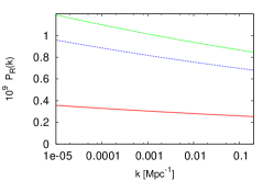
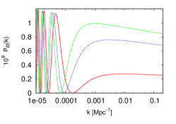
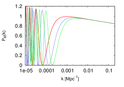
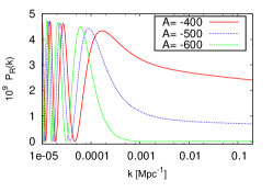
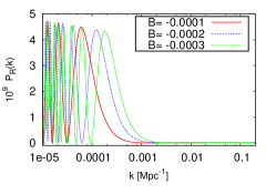
The effect on the predicted primordial power spectrum using both the Newtonian collapse and Wigner collapse schemes is showed in Fig. (1). It is found to be essentially a power-law with superimposed oscillations due to the $\mathcal{B}$ parameter. Indeed, the parameter $\mathcal{A}$ determines the amplitude of the spectrum (see the left and middle panels), while the parameter $\mathcal{B}$ influences the oscillations frequency (see the right panel) and determines the scale where the spectrum recovers the familiar $k^{n_{s}-1}$ form of the standard scenario. We note the difference in amplitude oscillation between the two schemes: using the same values of $\mathcal{A}$ and $\mathcal{B}$ the Newtonian collapse curves oscillates between [$0:1.2$] while the Wigner collapse curve covers the amplitude range [$0:5$]. Finally, we note the different behavior between the two parameterisations in the middle panel: while the Newtonian case approaches the power-law behavior from low values of the primordial spectrum, the Wigner collapse scheme behaves the other way around. This is due to the particular choice of the $\mathcal{A}$ value, i.e. theWigner scheme recovers the same Newtonian shape for $A=-800$.

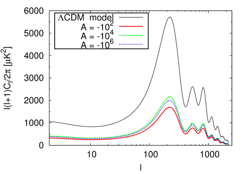
Next, we show the effects of assuming the collapse hypothesis for both the schemes considered in this paper on the CMB temperature auto-correlation angular power spectra. When the collapse parameter $\mathcal{B}=0$, as discussed before, we recover the standard $\Lambda$CDM model prediction unless a normalization factor. As a consequence the collapse parameter $\mathcal{A}$ will be highly degenerate with the scalar amplitude $A_{s}$. Furthermore, Figure (2) shows that the amplitude factor varies with different values of the collapse parameter $\mathcal{A}$ and we verified that the curves overlap within a normalization. It is worth mentioning that such a variation is highly non-linear.

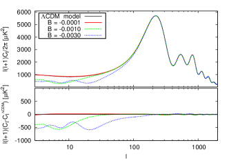
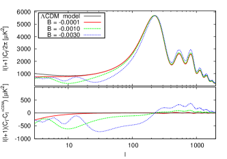
In Figure (3) we show the temperature auto-correlation (TT) power spectrum for a fixed value of $\mathcal{A}$ and different values of the collapse parameter $\mathcal{B}$. The value of $A_{s}$ is settled in each case in order to match the maximum of the first Doppler peak with the reference model one, namely the best fit $\Lambda$CDM model obtained by the Planck collaboration Ade et al. (2015). We can see that the value of the collapse parameter $\mathcal{B}$ affects the low multipole region. Besides, as the absolute value of $\mathcal{B}$ increases, the change takes the form of oscillations while as the value of $\mathcal{B}$ approaches to $0$ the shape of the spectrum approaches to the reference model one. Furthermore, we also analyzed the $EE$ and $TE$ angular power spectra and found only a tiny variation at low multipoles with respect to the reference model. On the other hand, for the Wigner scheme, we note a change in the height of the secondary peaks for increasing values of $\mathcal{B}$. This is due to a more sensitivity with the variations in the collapse parameter $\mathcal{B}$ of the latter with respect to the Newtonian scheme. In other words, the Newtonian scheme shows the same behaviour when bigger values of $\mathcal{B}$ are assumed. In agreement with the growth in high multipoles for increasing values of $\mathcal{B}$, we find small increases in the $EE$ and $TE$ power spectra.

IV Analysis Method

In order to compute the CMB anisotropies spectrum for given values of the collapse schemes parameters, we use a modified version of the CAMB (Lewis et al. (2000)) code to include the primordial power spectrum of the collapse models. We perform a Monte Carlo Markov chain analysis using the available package CosmoMC Lewis and Bridle (2002) and implement the nested sampling algorithm of Multinest code Feroz et al. (2009); Feroz and Hobson (2008); Feroz et al. (2013) to obtain our results and calculate the Bayesian evidence factor. In our Bayesian analysis we use the most accurate Importance Nested Sampling (INS) Cameron and Pettitt (2013); Feroz et al. (2013) instead of the vanilla Nested Sampling (NS), requiring a INS Global Log-Evidence error of $\leq 0.02$ .

Figure 4: Behaviour of the collapse parameter $\mathcal{A}$ with the primordial scalar amplitude $A_{s}$ for the Newtonian scheme model. In the left we show the relation in the $\mathcal{A}$ range [$-10^{-7}$ : $-10$] and the zoom in the $\mathcal{A}$ range [$-800$ : $-400$]. In the right we plot the progressive zoom in the $\mathcal{A}$ range [$-665$ : $-645$]. The reference green line draws the $\Lambda$CDM best fit value.

We consider extensions of the minimal $\Lambda$CDM model, adding the collapse schemes parameters $\mathcal{A}$ and $\mathcal{B}$ to the usual set of cosmological parameters: the baryon density, $\Omega_{b}h^{2}$, the cold dark matter density, $\Omega_{c}h^{2}$, the ratio between the sound horizon and the angular diameter distance at decoupling, $\theta$, the optical depth, $\tau$, the primordial scalar amplitude, $A_{s}$, and the primordial spectral index $n_{s}$. We consider purely adiabatic initial conditions, fix the sum of neutrino masses to $0.06\leavevmode\nobreak\ eV$ , and limit the analysis to scalar perturbations with $k_{0}=0.05$ $\rm{Mpc}^{-1}$. We also vary the nuisance foregrounds parameters Aghanim et al. (2015).

In our analysis we use the CMB data set from the latest Planck Collaboration release Ade et al. (2015), considering the high-$\ell$ Planck temperature data (in the range of $30<\ell<2508$) from the 100-,143-, and 217-GHz half-mission T maps, and the low-P data by the joint TT,EE,BB and TE likelihood (in the range of $2<\ell<29$). High-$\ell$ polarization data are not used since, as shown in the previous section, the analyzed collapse time expression affects only low multipoles, in both temperature and polarization spectra, recovering the $\Lambda$CDM behavior at small scales.

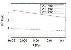
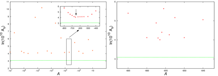
We work with flat priors for the cosmological parameters, and assume sharp prior intervals for the collapse parameter $\mathcal{A}$ . As seen in Figs. (1) and (2) , the $\mathcal{A}$ parameter just sets the primordial spectrum amplitude, which means that it is highly degenerate with the $A_{s}$ parameter. Furthermore, the spectrum amplitude value is significantly sensitive to variations of $\mathcal{A}$ . In Fig. (4) we show a progressive zoom in the range values of $\mathcal{A}$ , with respect to the $A_{s}$ parameter for the Newtonian scheme. Each point in the plot represents the combination of these parameters that assures the best fit to the current data. We can see that the $A_{s}$ value oscillates even with a smaller variation of $\mathcal{A}$ , generating significant computational problems. Testing several values for the $\mathcal{A}$ parameter, we select an interval of values which satisfies the condition for the conformal collapse time $\eta_{c}^{k}<0$ and minimizes the variation of the $A_{s}$ from the $\Lambda$CDM model value. In the same fashion, we perform the selection of the $\mathcal{A}$ value for the Wigner scheme (not shown in the figure). We also limit $\mathcal{B}$ into small values, since we also have a particular interest in studying features at low multipoles. We consider the interval of values shown in Tab. 1, however, worth mentioning that we have also explored different ranges of $\mathcal{B}$ values, e.g., $\lesssim\mathcal{B}=-3\times 10^{-3}$, which are strongly ruled out by the current data. Indeed, the increased sensitivity of the Wigner scheme discussed in the previous section is the reason why we considered a more stringent prior on $\mathcal{B}$ for this model.

In order to make an appropriate comparison between the collapse model and the standard $\Lambda{CDM}$ model predictions for the CMB angular power spectrum, we use the Bayesian model comparison, that is a very powerful tool to reward the models that fit well the data exhibiting strong predictivity, while models with a large number of free parameters, not required by the data, are penalised for the wasted parameter space. The Bayesian evidence $\mathcal{E}$ is defined as the marginal likelihood for the model $M_{i}$:

Parameter	Newtonian scheme	Wigner scheme
$\mathcal{A}$	[$-656.99$ : $-656.93$]	[$-800.05$ : $-800.00$]
$\mathcal{B}$	[$-5\times 10^{-4}$ : $0$]	[$-2.5\times 10^{-4}$ : $0$]

Table 1: Priors on the Newtonian and Wigner collapse scheme parameters considered in the analysis.

$$\mathcal{E}_{M_{i}}=\int d\theta p(x|\theta,M_{i})\pi(\theta|M_{i})\;.$$ (26)

where $x$ stands for the data, $\theta$ is the parameters vector and $\pi(\theta|M_{i})$ the prior probability distribution function. The ratio of the Bayesian evidence of the two models (the so-called Bayes Factor) can be defined as:

$$\mathit{B}_{ij}=\frac{\mathcal{E}_{M_{i}}}{\mathcal{E}_{M_{j}}}\;,$$ (27)

where $M_{j}$ is the reference model. The more complicate model $M_{i}$ (e.g., the one with more parameters with respect to the reference model) inevitably leads to a higher likelihood, but the evidence will favor the simpler model if the fit is as nearly as good, through the smaller prior volume. We assume uniform (and hence separable) priors in each parameter, such that we can write $\pi(\theta|M)=(\Delta\theta_{1}\leavevmode\nobreak\ ...\leavevmode\nobreak\ \Delta\theta_{n})^{-1}$ and

$$\mathit{B}_{ij}=\frac{\int d\theta p(x|\theta,M_{i})}{\int d\theta^{\prime}p(x|\theta^{\prime},M_{j})}\frac{(\Delta\theta_{1}\leavevmode\nobreak\ ...\leavevmode\nobreak\ \Delta\theta_{n_{i}})}{(\Delta\theta^{\prime}_{1}\leavevmode\nobreak\ ...\leavevmode\nobreak\ \Delta\theta^{\prime}_{n_{j}})}\;.$$ (28)

The usual scale employed to judge differences in evidence from the models is the Jeffreys scale Jeffreys (1961) which gives empirically calibrated levels of significance for the strength of evidence. In this work we will use a revisited and more conservative version of the Jeffreys convention suggested in Trotta (2007) where $\ln\mathit{B}_{ij}=0-1$, $\ln\mathit{B}_{ij}=1-2.5$, $\ln\mathit{B}_{ij}=2.5-5$, and $\ln\mathit{B}_{ij}>5$ indicate an inconclusive, weak, moderate and strong preference of the model $M_{i}$ with respect to the model $M_{j}$. Note that, for an experiment which provides $\ln\mathit{B_{ij}}<0$, it means support in favour of the reference model $M_{j}$ (see ref. Trotta (2007); Santos et al. (2016) for a more complete discussion about this scale).

Table 2: $68\%$ confidence limits for the cosmological and collapse scheme parameters. The first columns-block refer to the minimal $\Lambda$CDM model; the second and third columns-block show the constraint on the Newtonian and Wigner scheme models; The $\Delta\chi^{2}_{best}$ and the $\ln{B}_{ij}$ refers to the difference with respect to the $\Lambda$CDM.

	$\Lambda$CDM model		Newtonian-scheme		Wigner-scheme
Parameter	mean	bestfit	mean	bestfit	mean	bestfit
$100\,\Omega_{b}h^{2}$	$2.222\pm 0.022$	$2.209$	$2.222\pm 0.020$	$2.221$	$2.222\pm 0.020$	$2.218$
$\Omega_{c}h^{2}$	$0.1197\pm 0.0021$	$0.1201$	$0.1201\pm 0.0020$	$0.1201$	$0.1202\pm 0.0019$	$0.1194$
$100\,\theta$	$1.04085\pm 0.00045$	$1.04114$	$1.04083\pm 0.00045$	$1.04075$	$1.04081\pm 0.00045$	$1.04069$
$\tau$	$0.077\pm 0.018$	$0.070$	$0.086\pm 0.018$	$0.087$	$0.086\pm 0.018$	$0.088$
$n_{s}$	$0.9654\pm 0.0059$	$0.9635$	$0.9611\pm 0.0056$	$0.9598$	$0.9603\pm 0.0058$	$0.9648$
$\ln 10^{10}A_{s}$	$3.088\pm 0.034$	$3.080$	$4.130\pm 0.021$	$4.140$	$2.850\pm 0.022$	$2.871$
$\mathcal{A}$	$-$	$-$	$-656.960\pm 0.017$	$-656.975$	$-800.025\pm 0.014$	$-800.045$
$100$ $\mathcal{B}$	$-$	$-$	$-0.0128\pm 0.0053$	$-0.0107$	$-0.011\pm 0.0044$	$-0.0069$
$\Delta\chi^{2}_{\rm best}$		$-$		$3.4$		$1.4$
$\ln\mathit{B}_{ij}$		$-$	$-1.95\pm 0.03$		$-0.23\pm 0.03$

Figure 5: $68\%$ and $95\%$ confidence regions for the cosmological parameters of the $\Lambda$CDM (black line), Newtonian scheme (red line) and Wigner scheme (blue line) models using the Planck TT+lowP data. The numerical results of these analyses are reported in Tab. 2.

V Results

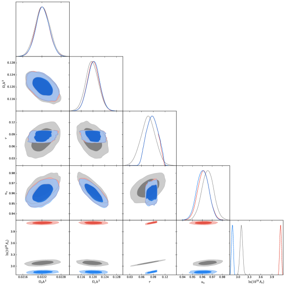
The main quantitative results of our analysis are shown in Tab. 2, where we analysed the $\Lambda$CDM model, the Newtonian collapse and the Wigner collapse schemes. We verify a significant agreement between the three models about the constraints on the cosmological parameters (see Fig. 5). For the collapse schemes, the $\tau$ parameter shows a preference for higher values while $n_{s}$ mean has a shift to lower values with respect to the $\Lambda$CDM model. The $\tau$ effect is due to the $\mathcal{A}$ parameter behaviour and its degeneracies with the magnitude of the primordial spectra. Also the $A_{s}$ parameter assume different values, with a slight deterioration of the error at one sigma.

Figure 6: One-dimensional posterior probability densities for the $\mathcal{B}$ parameter of the Newtonian scheme (red solid curve) and Wigner scheme (blue dotted).

Figure 7: $68\%$ and $99\%$ two-dimensional confidence region in the $n_{s}-\mathcal{B}$ of the Newtonian scheme (red) and Wigner scheme (blue) analysis.

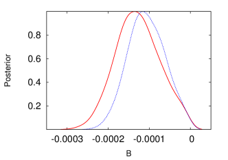
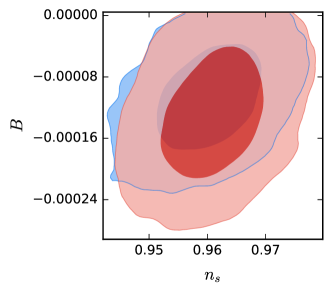
Remarkably, the data show a clear preference for non-zero values of $\mathcal{B}$ , with the power-law form (recovered with $\mathcal{B}=0$) being excluded from the data within two sigma. It can be clearly seen in Fig.(6), where the Gaussian $\mathcal{B}$ density posteriors distribution goes down for the zero value. The small improvement of the collapse scheme models on the $\chi^{2}$ values (with respect to the $\Lambda$CDM model) is displayed in the last rows of the Tab. 2. In what concerns the Bayesian analysis, the CMB data give an inconclusive Bayesian evidence of the Wigner scheme with respect to the standard scenario, which amounts to saying that the $\Lambda$CDM model and the collapse Wigner scheme show the same Bayesian evidence. On the other hand, the Newtonian scheme model is weakly disfavoured with respect to the $\Lambda$CDM model, with $\mathit{\ln B}_{ij}=-1.95\pm 0.03$. For completeness, we show in Fig.(7) the parameter space of $n_{s}$ and $\mathcal{B}$ for both collapse schemes. We can see that the Wigner scheme constrains a smaller volume with respect to the Newtonian case, which may explain the difference of values of the Bayesian evidence, according to Eq. (28). We recall that the collapse models are penalized by the Bayesian analysis for having two extra parameters compared to the minimal standard $\Lambda$CDM model. However, due to the high non-linearity of the collapse parameter $\mathcal{A}$, results shown in Table 2 should be regarded as the best fit for the Newtonian and Wigner schemes within the range $[-1000,0]$. Therefore, we can not reach any fair conclusion about the goodness of these models beyond this range of $\mathcal{A}$. This can be clearly seen in Table 3, where we report the results obtained when two different values of $\mathcal{A}$ are considered for the Newtonian model. For completeness, we also report in Tables 2 and 3 the improvements in $\Delta\chi^{2}$ for the best fit collapse models with respect to the $\Lambda$CDM.

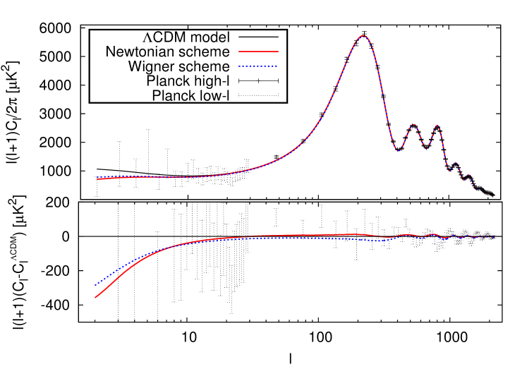
Finally, in Fig.(8) we show the anisotropy temperature power spectrum for the best fit values of the analysed models. Clearly, the collapse scheme scenarios are able to predict modifications in the low-$\ell$ region of the spectrum, which is not only in agreement with the data but also may be a possible explanation for the well-known lack of power at high scale ($\ell<20$) Ade et al. (2015); Copi et al. (2015).

Table 3: $68\%$ confidence limits the Newtonian scheme model fixing $\mathcal{A}$ $=50$ and $\mathcal{A}$ $=660$. The $\Delta\chi^{2}_{best}$ and the $\ln{B}_{ij}$ refers to the difference with respect to the $\Lambda$CDM model and a negative value for the $\Delta\chi^{2}_{best}$ means a lower value for the $\Lambda$CDM model.

	$\mathcal{A}$ = 50		$\mathcal{A}$ = 660
Parameter	mean	bestfit	mean	bestfit
$100\,\Omega_{b}h^{2}$	$2.222\pm 0.021$	$2.222$	$2.222\pm 0.021$	$2.209$
$\Omega_{c}h^{2}$	$0.1192\pm 0.0020$	$0.1197$	$0.1201\pm 0.0020$	$0.1213$
$100\,\theta$	$1.04091\pm 0.00045$	$1.04126$	$1.04084\pm 0.00045$	$1.04066$
$\tau$	$0.084\pm 0.018$	$0.072$	$0.087\pm 0.018$	$0.085$
$n_{s}$	$0.9697\pm 0.0056$	$0.9654$	$0.9616\pm 0.0056$	$0.9580$
$\ln 10^{10}A_{s}$	$4.073\pm 0.0168$	$4.058$	$4.070\pm 0.0170$	$4.063$
$100\,\ \mathcal{B}$	$-0.0223\pm 0.0131$	$-0.0003$	$-0.0149\pm 0.0060$	$-0.0195$
$\Delta\chi^{2}_{\rm best}$		$-0.6$		$3.4$
$\ln\mathit{B}_{ij}$	$-3.32\pm 0.02$		$-1.89\pm 0.02$

Figure 8: Anysotropy power spectrum for the $\Lambda$CDM (black line), the Newtonian (red solid line) and the Wigner scheme models (blue dotted line) for the best fit values reported in Tab.2. In the bottom panel, the differential plot with respect to the $\Lambda$CDM best fit curve.

VI Conclusions

Observations of the CMB radiation are one of the most powerful tools to study the physics of the early universe. Starting with COBE’s groundbreaking detection in the early nineties, the past two decades witnessed a great improvement in the measurements of the CMB fluctuations, which are now capable of ruling out theoretical models of inflation as well as some their alternatives.

In this paper, we have studied the phenomenological predictions of the collapse models developed in Ref. León et al. (2015a) considering only the case where the collapse happens before the horizon crossing. We have assumed a more predictive parameterisation for the collapse time $\eta_{c}^{k}$, i.e., $\eta_{c}^{k}=\frac{A}{k}+\frac{B}{k^{2}}$, which is able to fit the observed lack of power at low multipoles of the CMB temperature auto-correlation angular power spectrum. We have performed a statistical analysis to test the observational viability of the so-called Newtonian and Wigner scheme scenarios in the light of the most recent CMB data, as recently reported by the Planck Collaboration. In order to compare the predictivity power of these models with respect to the standard $\Lambda$CDM model, we have also performed a MCMC analysis and calculated the Bayesian evidence of each model.

The results, detailed in Sec. V, show that collapse inflationary models can explain the current CMB data. Furthermore, we have obtained very restrictive bounds on the collapse parameter $\mathcal{B}$ and shown that its value is different from 0 at $2\sigma$ level. On the other hand, the values obtained for the usual cosmological parameters are consistent within $1\sigma$ with those obtained by the Planck collaboration assuming a standard inflationary scenario. Finally, results from the Bayesian model comparison method show that the data can not distinguish between the $\Lambda$CDM and the Wigner scheme collapse model, while the former model is preferred over the Newtonian scheme collapse model.

References

- Perez et al. (2005) A. Perez, H. Sahlmann, and D. Sudarsky. On the quantum origin of the seeds of cosmic structure. Classical and Quantum Gravity, 23:2317–2354, August 2005.
- Sudarsky (2011) D. Sudarsky. Shortcomings in the Understanding of why Cosmological Perturbations Look Classical. International Journal of Modern Physics D, 20:509–552, 2011. doi: 10.1142/S0218271811018937.
- de Unánue and Sudarsky (2008) A. de Unánue and D. Sudarsky. Phenomenological analysis of quantum collapse as source of the seeds of cosmic structure. Physical Review D, 78(4):043510–+, August 2008. doi: 10.1103/PhysRevD.78.043510.
- León and Sudarsky (2010) G. León and D. Sudarsky. The slow-roll condition and the amplitude of the primordial spectrum of cosmic fluctuations: contrasts and similarities of the standard account and the ’collapse scheme’. Classical and Quantum Gravity, 27(22):225017, November 2010. doi: 10.1088/0264-9381/27/22/225017.
- Diez-Tejedor and Sudarsky (2012) A. Diez-Tejedor and D. Sudarsky. Towards a formal description of the collapse approach to the inflationary origin of the seeds of cosmic structure. JCAP, 7:045, July 2012. doi: 10.1088/1475-7516/2012/07/045.
- León et al. (2011) G. León, A. De Unánue, and D. Sudarsky. Multiple quantum collapse of the inflaton field and its implications on the birth of cosmic structure. Classical and Quantum Gravity, 28(15):155010, August 2011. doi: 10.1088/0264-9381/28/15/155010.
- Landau et al. (2012) S. J. Landau, C. G. Scóccola, and D. Sudarsky. Cosmological constraints on nonstandard inflationary quantum collapse models. Physical Review D, 85(12):123001, June 2012. doi: 10.1103/PhysRevD.85.123001.
- Landau et al. (2013) S. Landau, G. León, and D. Sudarsky. Quantum origin of the primordial fluctuation spectrum and its statistics. Physical Review D, 88(2):023526, July 2013. doi: 10.1103/PhysRevD.88.023526.
- León et al. (2015a) G. León, S. J. Landau, and M. P. Piccirilli. Inflation including collapse of the wave function: the quasi-de Sitter case. European Physical Journal C, 75:393, August 2015a. doi: 10.1140/epjc/s10052-015-3571-x.
- Cañate et al. (2013) P. Cañate, P. Pearle, and D. Sudarsky. Continuous spontaneous localization wave function collapse model as a mechanism for the emergence of cosmological asymmetries in inflation. Phys.Rev. D, 87(10):104024, May 2013. doi: 10.1103/PhysRevD.87.104024.
- Penrose (1996) Roger Penrose. On gravity’s role in quantum state reduction. Gen.Rel.Grav., 28:581–600, 1996. doi: 10.1007/BF02105068.
- Diosi (1987) L. Diosi. A Universal Master Equation for the Gravitational Violation of Quantum Mechanics. Phys.Lett., A120:377, 1987. doi: 10.1016/0375-9601(87)90681-5.
- Diosi (1989) L. Diosi. Models for universal reduction of macroscopic quantum fluctuations. Phys.Rev., A40:1165–1174, 1989.
- Ghirardi et al. (1986) G.C. Ghirardi, A. Rimini, and T. Weber. A Unified Dynamics for Micro and MACRO Systems. Phys.Rev., D34:470, 1986. doi: 10.1103/PhysRevD.34.470.
- Pearle (1989) Philip M. Pearle. Combining Stochastic Dynamical State Vector Reduction With Spontaneous Localization. Phys.Rev., A39:2277–2289, 1989. doi: 10.1103/PhysRevA.39.2277.
- Bassi and Ghirardi (2003) Angelo Bassi and Gian Carlo Ghirardi. Dynamical reduction models. Phys.Rept., 379:257, 2003. doi: 10.1016/S0370-1573(03)00103-0.
- Bassi et al. (2013) A. Bassi, K. Lochan, S. Satin, T. P. Singh, and H. Ulbricht. Models of wave-function collapse, underlying theories, and experimental tests. Reviews of Modern Physics, 85:471–527, April 2013. doi: 10.1103/RevModPhys.85.471.
- Kiefer and Polarski (2008) C. Kiefer and D. Polarski. Why do cosmological perturbations look classical to us? ArXiv e-prints, October 2008.
- Grishchuk and Sidorov (1990) L.P. Grishchuk and Yu.V. Sidorov. Squeezed quantum states of relic gravitons and primordial density fluctuations. Phys. Rev., D 42:3413–3421, 1990. doi: 10.1103/PhysRevD.42.3413.
- Adler (2001) S. L. Adler. Why Decoherence has not Solved the Measurement Problem: A Response to P. W. Anderson. eprint arXiv:quant-ph/0112095, December 2001.
- Schlosshauer (2004) Maximilian Schlosshauer. Decoherence, the measurement problem, and interpretations of quantum mechanics. Rev. Mod. Phys., 76:1267–1305, 2004. doi: 10.1103/RevModPhys.76.1267.
- Ade et al. (2015) P. A. R. Ade et al. Planck 2015 results. XIII. Cosmological parameters. 2015.
- Copi et al. (2015) Craig J. Copi, Dragan Huterer, Dominik J. Schwarz, and Glenn D. Starkman. Lack of large-angle TT correlations persists in WMAP and Planck. Mon. Not. Roy. Astron. Soc., 451(3):2978–2985, 2015. doi: 10.1093/mnras/stv1143.
- Bedingham (2011) D. J. Bedingham. Relativistic State Reduction Dynamics. Foundations of Physics, 41:686–704, April 2011. doi: 10.1007/s10701-010-9510-7.
- Pearle (2014) P. Pearle. A Relativistic Dynamical Collapse Model. ArXiv e-prints, December 2014.
- Lewis et al. (2000) A. Lewis, A. Challinor, and A. Lasenby. Efficient Computation of CMB anisotropies in closed FRW models. APJ, 538:473, 2000.
- Lewis and Bridle (2002) Antony Lewis and Sarah Bridle. Cosmological parameters from CMB and other data: A Monte Carlo approach. Phys. Rev., D66:103511, 2002. doi: 10.1103/PhysRevD.66.103511.
- Feroz et al. (2009) F. Feroz, M. P. Hobson, and M. Bridges. MultiNest: an efficient and robust Bayesian inference tool for cosmology and particle physics. Mon. Not. Roy. Astron. Soc., 398:1601–1614, 2009. doi: 10.1111/j.1365-2966.2009.14548.x.
- Feroz and Hobson (2008) Farhan Feroz and M. P. Hobson. Multimodal nested sampling: an efficient and robust alternative to MCMC methods for astronomical data analysis. Mon. Not. Roy. Astron. Soc., 384:449, 2008. doi: 10.1111/j.1365-2966.2007.12353.x.
- Feroz et al. (2013) F. Feroz, M. P. Hobson, E. Cameron, and A. N. Pettitt. Importance Nested Sampling and the MultiNest Algorithm. 2013.
- Cameron and Pettitt (2013) Ewan Cameron and Anthony Pettitt. Recursive Pathways to Marginal Likelihood Estimation with Prior-Sensitivity Analysis. 2013.
- Aghanim et al. (2015) N. Aghanim et al. Planck 2015 results. XI. CMB power spectra, likelihoods, and robustness of parameters. Submitted to: Astron. Astrophys., 2015.
- Bennett et al. (2013) C. L. Bennett et al. Nine-Year Wilkinson Microwave Anisotropy Probe (WMAP) Observations: Final Maps and Results. Astrophys. J. Suppl., 208:20, 2013. doi: 10.1088/0067-0049/208/2/20.
- Haslam et al. (1982) C. G. T. Haslam, C. J. Salter, H. Stoffel, and W. E. Wilson. A 408 MHz all-sky continuum survey. II. The atlas of contour maps. Astron. Astrophys. Suppl. Ser., 47:1–142, 1982.
- Jeffreys (1961) H. Jeffreys. Theory of probability. 3rd edn. OUP, 1961.
- Trotta (2007) Roberto Trotta. Applications of Bayesian model selection to cosmological parameters. Mon. Not. Roy. Astron. Soc., 378:72–82, 2007. doi: 10.1111/j.1365-2966.2007.11738.x.
- Santos et al. (2016) B. Santos, N. Chandrachani Devi, and J. S. Alcaniz. Bayesian comparison of non-standard cosmologies using type Ia supernovae and BAO data. 2016.
- León et al. (2015b) G. León, L. Kraiselburd, and S. J. Landau. Primordial gravitational waves and the collapse of the wave function. Phys. Rev. D, 92(8):083516, October 2015b. doi: 10.1103/PhysRevD.92.083516.