Density propagator for many-body localization: finite size effects, transient subdiffusion, and exponential decay

Abstract

We investigate charge relaxation in quantum-wires of spin-less disordered fermions ($t{-}V$-model). Our observable is the time-dependent density propagator, $\Pi_{\varepsilon}(x,t)$, calculated in windows of different energy density, $\varepsilon$, of the many-body Hamiltonian and at different disorder strengths, $W$, not exceeding the critical value $W_{\text{c}}$. The width ${\Delta x}_{\varepsilon}(t)$ of ${\Pi}_{\varepsilon}(x,t)$ exhibits a behavior $d\ln{\Delta x}_{\varepsilon}(t)/d\ln t{=}\beta_{\varepsilon}(t)$, where the exponent function $\beta_{\varepsilon}(t){\lesssim}1/2$ is seen to depend strongly on $L$ at all investigated parameter combinations. (i) We confirm the existence of a region in phase space that exhibits subdiffusive dynamics in the sense that ${\beta}_{\varepsilon}(t){<}1/2$ in large window of times. However, subdiffusion might possibly be transient, only, finally giving way to a conventional diffusive behavior with ${\beta}_{\varepsilon}{=}1/2$. (ii) We cannot confirm the existence of many-body mobility edges even in regions of the phase-diagram that have been reported to be deep in the delocalized phase. (iii) (Transient) subdiffusion $0<\beta_{\varepsilon}(t)\lesssim 1/2$, coexists with an enhanced probability for returning to the origin, ${\Pi}_{\varepsilon}(0,t)$, decaying much slower than $1/{\Delta x}_{\varepsilon}(t)$. Correspondingly, the spatial decay of ${\Pi}_{\varepsilon}(x,t)$ is far from Gaussian being exponential or even slower. On a phenomenological level, our findings are broadly consistent with effects of strong disorder and (fractal) Griffiths regions.

Introduction. The discovery of many-body localization (MBL) has attracted a considerable attention over recent years and gave rise to a new research field Basko et al. (2006); Gornyi et al. (2005); Nandkishore and Huse (2015); Altman and Vosk (2015); Vasseur and Moore (2016). An analytical proof of MBL has been given with minimal assumptions in spin-chains with random local interactions Imbrie (2016). Such MBL-phases are characterized by the absence of transport and thermalization Pal and Huse (2010); Canovi et al. (2011); Luitz et al. (2015), which has been attributed to a set of quasi-local integrals of motion Serbyn et al. (2013); Huse et al. (2014); Chandran et al. (2014); Ros et al. (2015). Anticipating that these integrals of motion adiabatically connect to their non-interacting analogues, it is perhaps natural to assume that there should be an adiabatic connection between localized eigenstates as well Bauer and Nayak (2013); Imbrie (2016).

The MBL-phase is distinguished from another phase that exhibits a degree of delocalization and which therefore is believed to be (thermal) ergodic Pal and Huse (2010); Canovi et al. (2012); Luca and Scardicchio (2013). The corresponding relaxation dynamics may not, however, reflect the simple diffusive behavior familiar from conventional metals. Instead, a subdiffusive scaling of the (spin-) density-correlations has been reported Bar Lev et al. (2015); Agarwal et al. (2015); Lev and Reichman (2016); Luitz et al. (2016); Khait et al. (2016); Žnidarič et al. (2016) (though some studies concluded differently Barišić et al. (2016); Steinigeweg et al. (2015)). It was understood to indicate Griffiths effects Vosk et al. (2015); Agarwal et al. (2015); Gopalakrishnan et al. (2015); Potter et al. (2015) near the MBL transition. Interestingly, it has been proposed that different behavior within these phases may also exist that exhibit diffusive relaxation of one conserved quantity (charge, energy or spin) and a subdiffusive behavior in another Vipin Kerala Varma and Scardicchio ; Žnidarič et al. (2016). Clearly, a coexistence of localized and delocalized behavior would be incompatible with generic expectations based on conventional mode-coupling ideas Gopalakrishnan et al. (2016).

Figure 1: A qualitative phase diagram of different dynamical regions in the disorder energy-density plane of the $t-V$-model. At disorder strength $W$ below the many-body localization transition $W_{\text{c}}$, we propose a transient subdiffusive, weakly ergodic dynamical regime with an anomalously slow decay of the return-probability.

The phase transition between the MBL- and the delocalized phase is not yet well understood. For instance, it has been shown that at very large values of the disorder, $W$, all eigenstates of the many-body Hamiltonian $\hat{H}(W)$ are localized Žnidarič et al. (2008); Pal and Huse (2010); Luitz et al. (2015); Kjäll et al. (2014); Serbyn et al. (2015), while with disorder dropping below a critical value $W{<}W_{c}$ a transition could occur below which $\hat{H}(W)$ supports a delocalized spectral density window  Oganesyan and Huse (2007); Kjäll et al. (2014); Luitz et al. (2015); Bera et al. (2015); Xu and Vavilov (2015); Mondragon-Shem et al. (2015); Kennes and Karrasch (2016) , see Fig. 1. At present, the width of this window is a matter of controversy. Recent numerical works on the random-field Heisenberg chain Luitz et al. (2015), the disordered Ising chain Kjäll et al. (2014), and recent work on Aubry-André model Li et al. (2015) were interpreted as giving evidence for the existence of a many-body mobility edge (MBME) that separates a band of delocalized states from localized band edges. Later authors have argued, however, that results can be significantly contaminated with finite size effects unless carefully extrapolated. For instance, the phase-boundary as found in Ref. Luitz et al. (2015) should be shifted to large disorder values as argued in Ref. Devakul and Singh (2015). In fact, the very existence of MBME was called in question by De Roeck et al., who suggested that the presence of a delocalized spectral window should imply the possibility for the formation of hot bubbles of electronic liquid that destabilize localizing processes in all spectral density windows De Roeck et al. (2016).

In this work, we investigate the charge propagation focussing on the delocalized region near the MBL transition. A common description of relaxation dynamics employs the density propagator, $\Pi(x,t)$, that takes a simple Gaussian shape for diffusive systems: $\Pi(x,t){=}e^{-\frac{1}{2}(x/\Delta x(t))^{2}}/\sqrt{2\pi}\Delta x(t),\Delta x(t){=}\sqrt{Dt}$, where $D$ is the diffusion constant. Aiming at mobility edges, we actually study a variant of it, ${\Pi}_{\varepsilon}(x,t)$, that resolves the contribution to $\Pi(x,t)$ stemming from many-body states with energy densities $\varepsilon$. We thus get access to the length scales relevant for the crossover physics, which allow us to carefully monitor finite size and finite time effects. In this way we go beyond previous studies.

We outline our results: (i) Within our observation window, ${\Pi}_{\varepsilon}(x,t)$ exhibits a very pronounced non-Gaussian spatial shape that decays in a (simple) exponential fashion or even slower. It is tempting to associate this finding with the stretched exponential behavior of correlations that has recently been proposed to exist due to fractal Griffiths regions in the localized phase near the phase boundary Zhang et al. (2016). (ii) Due to this peculiar shape of ${\Pi}_{\varepsilon}(x,t)$, the time dependence of its width $\Delta x_{\varepsilon}(t)$, is very sensitive to the system size, $L$. In order to highlight the effects of finite size in the time evolution, we investigate the exponent scaling function

$$\beta_{\varepsilon}(t)\equiv\frac{d\log\Delta x_{\varepsilon}(t)}{d\log t},$$ (1)

which at long times quantifies the rate of growth of $\Delta x_{\varepsilon}(t)\propto t^{{\beta}_{\varepsilon}(t=\infty)}$ and for diffusive systems ${\beta}_{\varepsilon}=1/2$. In the ergodic phase at intermediate times ${\beta}_{\varepsilon}(t)$ grows in a subdiffusive manner with values $\beta_{\varepsilon}(t){<}1/2$ consistent with the earlier reports Bar Lev et al. (2015); Agarwal et al. (2015); Luitz et al. (2016); Khait et al. (2016); Žnidarič et al. (2016). However with increasing time, ${\beta}_{\varepsilon}(t)$ becomes progressively $L$-dependent. At these longer times a similar tendency of growing ${\beta}_{\varepsilon}(t)$ (with $L$) is observed in all spectral windows – at low, intermediate and high energy density. This strong growths prevents us from confirming the existence of genuine subdiffusion that would exibit a time-independent exponent ${\beta}_{\varepsilon}{<}1/2$. We detect a slow growth of ${\beta}_{\varepsilon}(t)$ even in those regions of the phase diagram that have been identified previously as localized. Thus, the (delocalized) phase is larger than reported previously, which is associated with a very slow collective dynamics.

(iii) For the probability ${\Pi}_{\varepsilon}(0,t)$ to return to the origin one might have suspected ${\Pi}_{\varepsilon}(0,t){\propto}1/{{\Delta x}_{\varepsilon}(t)}$, suggesting ${\Pi}_{\varepsilon}(0,t)\propto t^{-{\beta}_{\varepsilon}(t=\infty)}$. Instead, our data indicates that the subdiffusive transients coexist with an elevated return probability consistent with (possibly transient) weakly ergodic sub-phases with fractal phenomenology, ${\Pi}_{\varepsilon}(0,t)\propto{\Delta x}_{\varepsilon}(t)^{-\alpha_{\varepsilon}}$ and $0\leq\alpha_{\varepsilon}<1$.

Model and Method. Like several works before Oganesyan and Huse (2007); Berkelbach and Reichman (2010); Luca and Scardicchio (2013); Luitz et al. (2015); Bera et al. (2015); Bar Lev et al. (2015); Bera and Lakshminarayan (2016); De Tomasi et al. (2016), we consider the $t{-}V$-model

$$\mathcal{\hat{H}}= -\frac{t_{\text{h}}}{2}\sum_{x=-L/2}^{L/2-2}\hat{c}^{\dagger}_{x}\hat{c}_{x+1}+h.c.+\sum_{x=-L/2}^{L/2-1}\mu_{x}\left(\hat{n}_{x}-\frac{1}{2}\right)$$

$$+V\sum_{x=-L/2}^{L/2-2}\left(\hat{n}_{x}-\frac{1}{2}\right)\left(\hat{n}_{x+1}-\frac{1}{2}\right),$$ (2)

where the summations are along an $L$-site wire, $x{=}1,\ldots,L$, with hopping ($t_{\text{h}}=1$) and interaction ($V$) between nearest neighbors, only; the uncorrelated on-site energies $\mu_{x}$ are being drawn from a box distribution $[-W,W]$. We work at a half filling and with open boundary conditions. For $V=1.0$, the MBL transition is believed to be at $W_{\text{c}}\approx 3.5$ Luitz et al. (2015). The specific correlator ${\Pi}_{\varepsilon}(x,t)$ that we are interested in has not yet been investigated; it is defined via its Fourier space representation :

$$\Pi_{\varepsilon}(q,t)=\overline{\Phi_{\varepsilon}(q,t)/\Phi_{\varepsilon}(q,t{=}0^{+})},$$ (3)

where the disorder average is denoted by the overline. $\Phi_{\varepsilon}(q,t)$ is the Fourier transform of the energy-projected density relaxation functions

$$\Phi_{\varepsilon}(x,t) = \left[\langle\hat{n}_{x}(t)\hat{n}_{0}\rangle_{\varepsilon}-\langle\hat{n}_{x}\rangle_{\varepsilon}\langle\hat{n}_{0}\rangle_{\varepsilon}\right]\Theta(t)\text{.}$$ (4)

The projection into a narrow spectral range near $\varepsilon$ is facilitated by taking the expectation value of an operator $\langle\hat{\mathcal{O}}\rangle_{\varepsilon}=\text{Tr}\hat{\mathcal{O}}\hat{\rho}(\varepsilon)$ with

$$\hat{\rho}({\varepsilon})=\mathcal{N}^{-1}\int_{\varepsilon-\Delta\varepsilon/2}^{\varepsilon+\Delta\varepsilon/2}d\varepsilon^{\prime}\sum_{\gamma}^{\mathcal{N}}|\gamma\rangle\delta(\varepsilon_{\gamma}-\varepsilon^{\prime})\langle\gamma|\text{,}$$ (5)

where $|\gamma\rangle$ denotes the eigenstates of the Hamiltonian (2) with energy-density $\varepsilon_{\gamma}{=}(E_{\gamma}{-}E_{\text{min}})/(E_{\text{max}}{-}E_{\text{min}})$, where $E_{\gamma}$ are the many-body energies and $E_{\text{max, min}}$ denote the extremal values of the energy spectrum. $\mathcal{N}$ represents the number of states in the energy density window $\Delta\varepsilon$, and it is exponentially large in $L$. By definition, $\Pi_{\varepsilon}(q{=}0,t){=}1$ and for a conventional diffusive system we have a Gaussian shape, $\Pi_{\varepsilon}(q,t){=}\exp(-(\Delta x_{\varepsilon}(t)q)^{2})\Theta(t)$, with $\Delta x_{\varepsilon}(t)=\sqrt{D_{\varepsilon}t}$. For the time evolution, Eq. (4), we employ a standard Chebyshev-polynomial propagation  Weiße et al. (2006); traces over operators are performed stochastically as averages over random state vectors. The approach owes its efficiency to the fact that disorder averages converge very rapidly with the number of random states. Details of the calculations and performance tests we relegate to the supplementary material.

Figure 2: (a1)-(a3) The time evolution of ${\Delta x}_{\varepsilon}(t)$ at $W{=}2.5$ and $V{=1}$ near the lower band-edge (upper row, $\varepsilon=0.1$) in the center region (center row, $0.5$) and near the upper band-edge (lower row, $0.875$) for system sizes $L=16,20,24$ (dashed traces blue, red, green). Also shown are non-interacting reference traces for $L{=}16,20$ ($V{=}0$, solid lines). (b1)-(b3) Re-plotting (a1)-(a3) as $d\ln\Delta x_{\varepsilon}(t)/d\ln t$ over $\Delta x_{\varepsilon}(t)/\Delta x_{\varepsilon}^{(0)}$ to highlight finite-size effects. Inset shows the blow up of the (b3) data for better visibility of trends including system sizes $L=16,18,20,22,24$ (bottom to top). (c1)-(c3) Probability to return to the origin. The legends in this column also give the three system sizes in units of the bare localization length. (In all calculation we fix the width of the energy window $\Delta\varepsilon=0.1$ sup .)

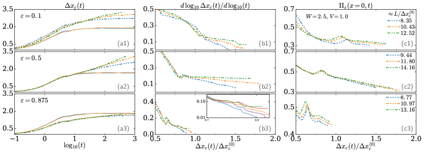
Results. We begin the analysis of the propagator ${\Pi}_{\varepsilon}(x,t)$ with its second moment in real space,

$${\Delta x}_{\varepsilon}(t)^{2}{=}\langle x^{2}\rangle_{\varepsilon}-\langle x\rangle_{\varepsilon}^{2}\text{,}\quad\langle x^{n}\rangle_{\varepsilon}=\sum\limits_{x=-L/2}^{L/2-1}x^{n}\ {\Pi}_{\varepsilon}(x,t).$$

Fig. 2-(a1-a3) show the ${\Delta x}_{\varepsilon}(t)$ at $W=2.5$ for both interacting ($V=1$, dashed line) and non-interacting ($V=0$, solid line) case for several values of energy densities ($\varepsilon=0.1,0.5,0.875$). For these parameters MBMEs have been reported near $\varepsilon\approx 0.2$ and near $0.8$ with a delocalized regime in between Luitz et al. (2015).

Figure 2-(a1-a3) carries several messages. (i) Finite size effects are very strong: the system size, $L$, exceeds the non-interacting standard deviation, ${\Delta x}_{\varepsilon}^{(0)}$ (saturation value in time), by a factor of 10-15 ($\approx L/{\Delta x}_{\varepsilon}^{(0)}$), but nevertheless the growth of ${\Delta x}_{\varepsilon}(t)$ changes with $L$ by as much as 30%. (ii) The interaction mediated delocalization process is very slow. Even after a time that typically corresponds to 0.1% of the inverse hopping $t^{-1}_{\text{h}}$ the width of the wavepacket has grown by less than a factor of two as compared to ${\Delta x}_{\varepsilon}^{(0)}$. (iii) Depending on the spectral window, the transient dynamics is quite different. In particular, the spreading of ${\Pi}_{\varepsilon}(x,t)$ is enhanced by the interactions at low energy densities while it is hindered at high densities as compared to the non-interacting reference case.

Figure 3: (a1)-(a3) The density propagator ${\Pi}_{\varepsilon}(x,t)$ in the delocalized regime ($\varepsilon{=}0.1,0.5,0.875$, $W{=}2.5$, $L{=}24$) at two times $t{=}40,100$. The log-normal plot illustrates non-Gaussian shape. Solid line in (a3) shows a stretched exponential fit with an exponent $\approx 0.7$. (b1)-(d3) The corresponding memory kernel $\kappa_{\varepsilon}(q,t){=}q^{2}/({\Pi}_{\varepsilon}^{-1}(q,t)-1)$, see also (6), for the case without (b1)-(b3) and with interactions (c1)-(d3). The structure at larger wavenumbers illustrates the (non-exponential) short-distance behavior. The absence of effects in time (and system size, not shown) highlights the localized character of the non-interacting kernel $\kappa_{\varepsilon}^{(0)}$. In contrast, the evolution of the interacting kernel is the hallmark of delocalization. (d1)-(d3) Shows the $L$-dependence of $\kappa_{\varepsilon}(t)$.

Flowing exponent – ${\beta}_{\varepsilon}(t)$. To quantify the time dependence of ${\Delta x}_{\varepsilon}(t)$, we study the ${\beta}_{\varepsilon}(t)$ as defined in Eq. (1). Fig. 2-(b1-b3) shows the ${\beta}_{\varepsilon}-$function as a function of ${\Delta x}_{\varepsilon}(t)/{\Delta x}_{\varepsilon}^{(0)}$. It very clearly highlights the fact that beyond a certain transient time, $\tau_{\varepsilon}$ (set by the kink position), a slow dynamics sets in which reveals itself by a high degree of sensitivity to the system size, $L$. Moreover, as is seen in Fig. 2-(b1-b3) all traces of ${\beta}_{\varepsilon}(t)$ experience a kink with a position evolving with the energy density $\varepsilon$ that does not collapse after rescaling of the abscissa with ${\Delta x}_{\varepsilon}^{(0)}$.

While the range of $L$-values available to us is not sufficient to study the asymptotic limit (in $L$ and $t$), our data nevertheless gives a non-vanishing lower bound for ${\beta}_{\varepsilon}(t)$ and hence indicates delocalization, at least near the band-center. With this caveat, we notice that the qualitative behavior seen in all energy ranges is the same: With $L$ increasing, there is a pronounced trend for ${\beta}_{\varepsilon}(t)$ to grow (at fixed long time), see Fig. 2-(b1-b3) and inset. Strictly speaking, we thus find no evidence for an upper bound to ${\beta}_{\varepsilon}$ below the diffusion limit $1/2$, i.e. for genuine subdiffusion. Moreover, the growth (with $L$) being similar in all energy windows, we also find no evidence for the existence of a many-body mobility edge at $W{=}2.5$. The picture is similar for other choices of $W~{}(\lesssim 3.0)$ sup . At larger disorder and close to the transition, $W{\approx}W_{\text{c}}$, the situation is numerically less conclusive due to residual statistical noise. To account for this in Fig. 1, this region of the phase-diagram has been left uncolored (white).

Return probability – ${\Pi}_{\varepsilon}(x{=}0,t)$. In one dimensional diffusive systems the return probability associated with a spreading wavepacket relates to the variance ${\Pi}_{\varepsilon}(0,t)\sim 1/{\Delta x}_{\varepsilon}(t)$, merely stating that the wavepacket is internally homogeneous. The data displayed in Fig. 2-(c1 - c3) does not adhere to this fundamental idea: ${\Pi}_{\varepsilon}(0,t)$ is close to stationary and therefore does not follow the $1/{\Delta x}_{\varepsilon}$ law, most clearly seen in the low and high energy density regimes. This observation finds a natural explanation adopting the idea of strong disorder induced fractality. Indeed it is well known that in the presence of (multi-)fractality the return-probability can be enhanced, $\Pi_{\varepsilon}(0,t)\propto{\Delta x}_{\varepsilon}^{-\alpha_{\varepsilon}}$, with $0\leq\alpha_{\varepsilon}<1$ Ketzmerick et al. (1997). A very slowly decaying return probability can therefore also indicate a fractal-type behavior, i.e. $\alpha_{\varepsilon}$ being significantly smaller than unity. Unfortunately, it is very challenging to extract $\alpha_{\varepsilon}$ reliably from our data, because our observation window for ${\Delta x}_{\varepsilon}(t)/{\Delta x}_{\varepsilon}^{(0)}$ does not exceed a factor 2-3.

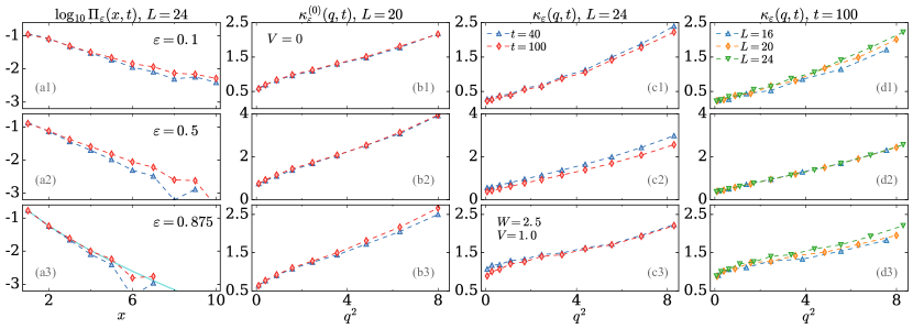
Density propagator – ${\Pi}_{\varepsilon}(x,t)$. To understand the transient sub-diffusive behavior further, here we look at the time dependence of the full distribution function, ${\Pi}_{\varepsilon}(x,t)$, both in real and $q$-space. Fig. 3-(a1-a3) displays a density-propagator ${\Pi}_{\varepsilon}(x,t)$ that is far from Gaussian. To highlight its shape (curvature at small $q$,large $x$) we rewrite $\Pi_{\varepsilon}(q,t)$ employing an (inverse) memory kernel, $\kappa_{\varepsilon}(q,t)$,

$$\Pi_{\varepsilon}(q,t)=\left(1+q^{2}/\kappa_{\varepsilon}(q,t)\right)^{-1},$$ (6)

where $-\partial_{q}^{2}\Pi_{\varepsilon}(q,t)\rvert_{q=0}=2/\kappa_{\varepsilon}(0,t)\sim{\Delta x}_{\varepsilon}(t)^{2}$. A numerical example can be read off from Fig. 3-(b-c). It displays $\kappa_{\varepsilon}$ at three different energy densities at intermediate disorder strength $W{=}2.5$. Notice that the non-interacting kernel, $\kappa_{\varepsilon}^{(0)}(q,t)$, is rapidly growing with wavenumber, $q$ (see Fig. 3(b1-b3)). This behavior reflects the presence of a short-distance cutoff, $a$, such as the lattice constant, terminating the long-distance, exponential tail. It exists in a similar way also in the interacting kernels $\kappa_{\varepsilon}(q,t)$, see Fig. 3-(c-d)  .

Conclusions. In this work, we have considered the full space-time structure of the spectrally resolved density correlator, ${\Pi}_{\varepsilon}(x,t)$, allowing us to monitor finite size effects. (i) The processes that are characteristic of delocalized behavior are very slow. Even at observation times of order $10^{3}$ (in units of inverse hopping $t_{\text{h}}^{-1}$), ${\Pi}_{\varepsilon}(x,t)$ has spread over little more than the non-interacting length, ${\Delta x}_{\varepsilon}^{(0)}$. (ii) Although the system size exceeds ${\Delta x}_{\varepsilon}^{(0)}$ by a large factor, finite size effects are substantial reflecting a spreading of ${\Pi}_{\varepsilon}(x,t)$ that is far from Gaussian, possibly (stretched) exponential in the tails.

Because of strong finite-size effects, the exponents ${\beta}_{\varepsilon}(t)$ that describe the spreading dynamics of the variance of the density propagator, $d\ln{\Delta x}_{\varepsilon}(t)/d\ln t={\beta}_{\varepsilon}(t)$, are hard to quantify reliably. We are able to provide a lower bound for ${\beta}_{\varepsilon}(t)$ suggesting the absence of many-body mobility gaps in the $t-V$-model at values of $W$ not too close to the transition region – apparently consistent with recent analytical arguments De Roeck et al. (2016). Since we cannot provide an upper bound for ${\beta}_{\varepsilon}(t)<1/2$, we cannot confirm the existence of genuine subdiffusive behavior in the asymptotic limit; a logically possible alternative is a transient behavior with an effectively growing exponent ${\beta}_{\varepsilon}(t)$ that gradually converges to the diffusion limit $1/2$. Together with transient subdiffusive behavior, we observe a drastically enhanced return probability, which could be interpreted as $\Pi_{\varepsilon}(0,t)\propto{\Delta x}_{\varepsilon}^{-\alpha_{\varepsilon}}$ in accord with the assumptions of fractality induced by strong-disorder physics.

Based on these findings we propose the following scenario: There is a timescale $\tau_{\varepsilon}$ beyond which a slow dynamics kicks in together with diffusive behavior. Approaching the MBL transition from the delocalized side, this time scale diverges; simultaneously, ${\beta}_{\varepsilon}(t)$ at times $t{\lesssim}\tau_{\varepsilon}$ is rapidly decreasing, which might suggest a small value of ${\beta}_{\varepsilon}$ at the MBL transition. In this scenario, the critical fixed-point would carry excited states that exhibit phenomenological features reminiscent of (strong) multifractality Evers and Mirlin (2008).

We conclude with two remarks relating our work to the most recent literature. (a) Consistent with our findings, also Serbyn et. al. observe very strong finite size effects in their study of the Thouless energy Serbyn et al. (2016). Like us, they interpret their results as indicating that the system sizes are too short for observing the asymptotic thermalized behavior. Unlike us, they go a step further proposing that the numerical data at small system sizes (below $L{=}20$) already reveals hydrodynamic properties of the critical fixed point, such as multifractality. This conclusion for us is difficult to draw, because one would expect system-size independent exponents in the critical window, which we don’t observe. (b) Recent studies of Anderson localization of random regular graphs (RRG) reveal a slow flow with system size out of a (quasi-)multifractal into an ergodic regime García-Mata et al. (2016); Tikhonov et al. (2016). When interpreting ${\Delta x}_{\varepsilon}(t)$ as an effective system size, then the transient subdiffusive behavior observed by us finds a natural interpretation within the RRG-perspective.

Acknowledgments. Discussions with I. Gornyi, A. D. Mirlin and D. Polyakov are gratefully acknowledged. SB and GDT also thank M. Heyl for discussions. The project was supported by DFG under projects EV30/7-1 and EV30/11-1. SB acknowledges support from the ERC starting grant QUANTMATT NO. 679722.

Additional material for ‘Density propagator for many-body localization: finite size effects, transient subdiffusion, and exponential decay’

Appendix A Validation of the numerical method

The energy-projected density relaxation function is the main object studied in this work. It is defined as

$$\Phi_{\varepsilon}(x,t)=\left[\langle\hat{n}_{x}(t)\hat{n}_{0}\rangle_{\varepsilon}-\langle\hat{n}_{x}\rangle_{\varepsilon}\langle\hat{n}_{0}\rangle_{\varepsilon}\right]\Theta(t)\text{,}$$ (S1)

where $\langle\hat{\mathcal{O}}\rangle_{\varepsilon}=\text{Tr}\hat{\mathcal{O}}\hat{\rho}(\varepsilon)$, and $\hat{\rho}(\varepsilon)$ projects into a narrow spectral range near energy density $\varepsilon$ with width $\Delta\varepsilon$. To calculate the two-point space-time correlator (S1) for large systems ($L{=}24$) and long times (${\approx}10^{3}$), we use two approximations: (i) The energy projected trace denoted via the angular brackets $\langle\ldots\rangle_{\varepsilon}$ is evaluated stochastically, while (ii) the time evolution is performed employing a standard kernel-polynomial method based on Chebyshev polynomials. In this section, we detail and validate (i) and (ii), including data illustrating the convergence properties.

A.1 Chebyshev-representation of the density matrix $\hat{\rho}({\varepsilon})$

For numerical evaluation we represent the density matrix $\hat{\rho}({\varepsilon})$ as a simple function of the Hamiltonian $\mathcal{\tilde{H}}$ (and is rescaled between energy density $\{0,1\}$) in the following way,

$$\hat{\rho}(\varepsilon)=\frac{\mathscr{R}_{[\varepsilon-\Delta\varepsilon/2,\varepsilon+\Delta\varepsilon/2]}(\mathcal{\tilde{H}})}{\text{Tr}\,\mathscr{R}_{[\varepsilon-\Delta\varepsilon/2,\varepsilon+\Delta\varepsilon/2]}(\mathcal{\tilde{H}})},$$ (S2)

where $\mathscr{R}_{[a,b]}(x)$ is the box function of unit height in the interval $[a,b]$. We approximate $\hat{\rho}({\varepsilon})$ as a truncated Chebyshev series,

$$\hat{\rho}({\varepsilon})\approx\frac{\sum_{i=0}^{M}\mu_{i}T_{i}(\mathcal{\tilde{H}})}{\text{Tr}\sum_{i=0}^{M}\mu_{i}T_{i}(\mathcal{\tilde{H}})}$$ (S3)

where $\{T_{i}(x)\}$ denote the Chebyshev polynomials. $M$ denotes the order of the expansion taken sufficiently large ($M\geq 3000$) to assure convergence (S3) (see also Fig. S1 right panel). The expansion coefficients $\{\mu_{i}\}$ are given as follows: $\mu_{0}=\frac{1}{\pi}(\arccos{a}-\arccos{b})$, $\mu_{1}=\frac{1}{\pi}(\sqrt{1-a^{2}}-\sqrt{1-b^{2}})$, $\mu_{n\geq 2}=\frac{1}{n\pi}(\sin{(\arccos{nb})}-\sin{(\arccos{na})})$.

Figure S1: Convergence of the variance of the density propagator (defined explicitly in the main paper) with respect to the number of moments, $M$, used in the expansion (S3). $R$ defines the number of random vectors taken for the trace evolution (see text for definition). Only 16 disorder samples is taken for averaging.

In Fig. S1 we display the convergence of the time evolution of our main observable, the variance $\Delta x_{\varepsilon}(t)$, with respect to the number of moments in the sum (S3). For definition of the $\Delta x_{\varepsilon}(t)$, see main text.

A.2 Stochastic trace evaluation and convergence

Figure S2: Trace evaluation: comparison between exact and stochastic methods for ${\Pi}_{\varepsilon}(q,t)$ and $\Delta x_{\varepsilon}(t)$). (Parameters: $L=14$, middle of the band $\varepsilon=0.5$ and $W=3.0,V=1.0$). (a) Density propagator ${\Pi}_{\varepsilon}(q,t=40)$ in $q$-space for a single disorder realization. The (green) dots represent the exact data calculated using the full trace employing exact diagonalization; the dashed lines are evaluated with different number of random vectors $R=\{2,8,16\}$ (blue, black, red) employing the stochastic trace formula (S4). (b) Density propagator ${\Pi}_{\varepsilon}(q,t)$ averaged over 16 disorder realizations. As can be seen, the average of ${\Pi}_{\varepsilon}(q,t)$ over the disorder realization converges rapidly in the number $R$ of stochastic state vectors as opposed to ${\Pi}_{\varepsilon}(q,t)$ taken for a single disorder realization. (c),(d) A similar trend is also visible with real space data, here shown for the second moment of ${\Pi}_{\varepsilon}(x,t)$: $\langle\Delta x^{2}(t)\rangle$.

The expectation values $\langle\hat{\mathcal{O}}\rangle_{\varepsilon}$ have been calculated using stochastic trace evaluation. The idea is to represent a trace as an average over an ensemble of random state vectors $\{|r\rangle\}_{r=0}^{R}$:

$$\langle\hat{\mathcal{O}}\rangle_{\varepsilon}\sim\frac{1}{R}\sum_{r=0}^{R-1}\langle r|\hat{\rho}({\varepsilon})\hat{\mathcal{O}}|r\rangle,\quad\text{with}\;R\gg 1.$$ (S4)

Figure S3: Shows the variance $\Delta x_{\varepsilon}(t)$ for three trace vectors $R=\{2,8,16\}$ after a small disorder averaging $N_{\text{d}is}=32$ for two different system sizes $L=16,20$.

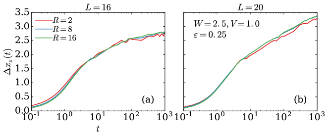
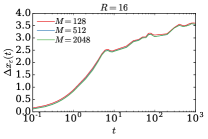
Truncating the sum at an upper cutoff, $R$, for global variables the relative error decays as $1/\sqrt{DR}$, $D$ denoting the dimension of the Hilbert space. Hence, the stochastic trace evaluation is most efficient in very high dimensions (for variables that sample the full system size). In our case, $D$ is exponentially large in the system size, $L$, and is given by ${L\choose N}$, $N$ being the particle number. For smaller system size, $L\lesssim 20$, we typically use $R{=}16$ random state vectors, while for larger system sizes we only keep $R{=}2$. The convergence properties are illustrated in Fig. S2-(a). The plot displays a comparison between the stochastic trace estimate and an exact trace evaluation. As is seen there, the convergence properties of the distribution ${\Pi}_{\varepsilon}(q,t)$ with $R$ are actually quite poor; at $R{=}16$ deviations are still of the order of a few percent.

however, note that the convergence with $R$ is drastically improved for the traces averaged over the disorder ensemble, i.e. for $\overline{\langle\hat{\mathcal{O}}\rangle_{\varepsilon}}$ Fig. S2-(b) shows that even for a relatively small ensemble of $N_{\text{dis}}{=}16$ samples a good convergence is reached already with $R{=}2$. The same behavior is seen at all times. To illustrate this we display similar data also for the variance, $\Delta x_{\varepsilon}(t)$. Again, the disorder averaged variance converges very rapidly with the number $R$ of random states kept for the trace evaluations.

Figure S3 further illustrates the dependence of the variance on the averaging over trace vectors, now for two larger system sizes. As is obvious from both plots, the variance is well approximated at all times with only a small number of trace vectors. With increasing system size and improving disorder average the trace approximation becomes progressively efficient. This is because the error scales as $\propto 1/\sqrt{D}$, where $D$ is the dimension of the Hilbert space, which increases exponentially fast with the system size $L$.

Figure S4: Evolution of the exponent $\beta_{\varepsilon}(t)=d\ln\Delta x_{\varepsilon}(t)/d\ln t$ for different values of the width of the energy density $\Delta\varepsilon$ for $L=16$ and disorder strengths $W=\{2.0,2.5,3.0,3.5\}$ and $\varepsilon=0.25$.

A.3 Time evolution: Chebyshev expansion

The time evolution of the operators has been preformed relying once more the standard Kernel polynomial techniques Weiße et al. (2006) employing Chebyshev expansions of the exponential of the $\mathcal{\hat{H}}$:

$$U(t)\approx e^{-ibt}\sum_{k=0}^{N}\mu_{k}T_{k}(\tilde{\mathcal{H}});\qquad\mu_{k}=(-i)^{k}J_{k}(at),$$ (S5)

where $\tilde{\mathcal{H}}=\frac{\mathcal{\hat{H}}{-}b}{a}$ denotes the rescaled Hamiltonian; $a=(E_{\text{max}}{-}E_{\text{min}})/2$, $b=(E_{\text{max}}{+}E_{\text{min}})/2$ are the scaling factors and $J_{k}(x)$ denotes the Bessel function of order $k$. We typically take $N\gtrsim 2at$ to ensure convergence Weiße and Fehske (2008) of the truncated Chebyshev series ($T_{k}(x)$). Eq. (S5) only requires sparse matrix multiplications. The iterative scheme scales as $\mathcal{O}(M)$ as compare to exact diagonalization which is $\mathcal{O}(M^{3})$, $M$ denoting the dimension of $\mathcal{\hat{H}}$. Therefore, system sizes up to $L=24$ can be treated for times of the order $\approx 10^{3}$ (in units of inverse hopping $t_{\text{h}}=1.0$).

A.4 Dependence on $\Delta\varepsilon$

We have ascertained that our choice of the width $\Delta\varepsilon$ of the energy-density shell was sufficiently narrow so that our results for ${\Pi}_{\varepsilon}(x,t)$ and its variance are (essentially) independent of it. In Fig. S4 we show the evolution of the exponent $\beta_{\varepsilon}(t)$ for two different values of the width $\Delta\varepsilon=0.1,0.2$ of the box function (S2) at energy density $\varepsilon=0.25$. The data is averaged over $\gtrsim 10^{4}$ disorder configurations. As is easily deferred from the figure, the curves are almost indistinguishable form each other. In all the data presented in the main part of the work we choose $\Delta\varepsilon=0.1$.

Appendix B Results: Dependence of $\beta_{\varepsilon}(t)$ on disorder and energy density

Figure S5: Time dependence of the exponent $\beta_{\varepsilon}(t)=d\ln\Delta x_{\varepsilon}(t)/d\ln t$ for different disorder $W=\{2.0,2.5,3.0,3.5\}$ and system sizes ($L{=}16,18,20,22$) at four different energy densities $\varepsilon=\{0.1,0.125,0.5,0.875\}$ with $\Delta\varepsilon=0.1$ and $V=1.0$. Inset: Shows the same data as fourth column but zoomed for better visibility of the trend in the data with increasing system sizes.

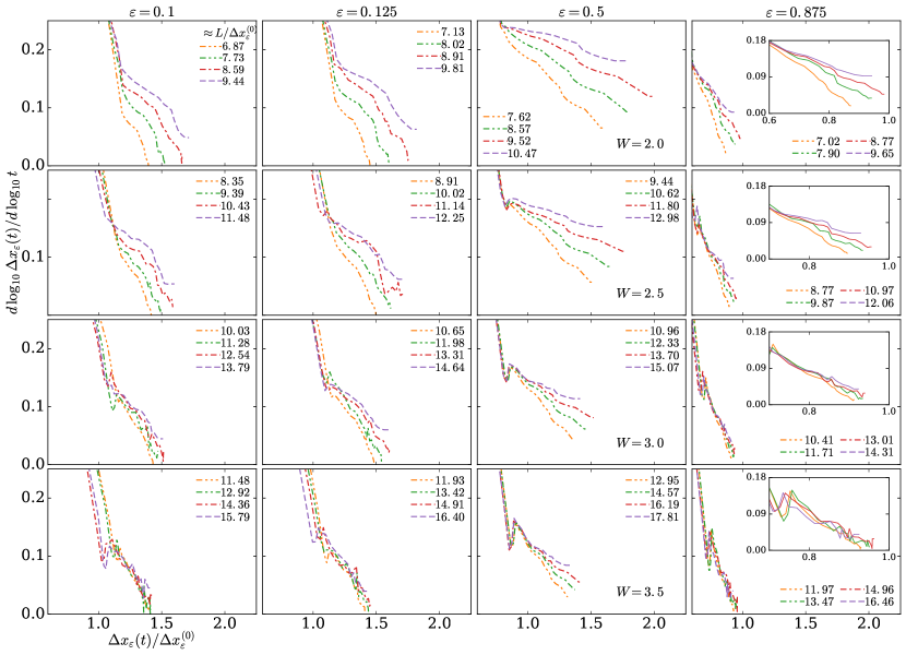
Fig. S5 shows the evolution of the $\beta_{\varepsilon}(t)$ over $\Delta x_{\varepsilon}(t)/\Delta x_{\varepsilon}^{(0)}$ for $L=\{16,18,20,22\}$, at four energy densities and four disorder values close to the many-body localization transition ($W=\{2.0,2.5,3.0,3.5\}$), which is believed to be around $W_{\text{c}}\approx 3.5$. For these data we usually perform around $10^{6}$ disorder realizations for small system sizes ($L\lesssim 20$), while for larger system sizes the data is averaged over around $10^{4}$ disorder samples.

$\varepsilon{=}0.5$,

Fig. S5 (3rd column): We start our discussion from the middle of the spectrum. In this regime the data clearly indicates that the dynamics is (transient) subdiffusive with an (effective) exponent, $\beta_{\varepsilon}(t)<1/2$, which depends strongly on system size $L$. The $L-$dependence is reflected via the upward movement of the $\beta_{\varepsilon}(t)$. We interpret this systematic trend as an indication to delocalization.

$\varepsilon=0.1,0.125$:

Fig. S5 (1st, 2nd column) shows the evolution of the exponent $\beta_{\varepsilon}(t)$ for different systems sizes in the low energy-density regime. Previous studies assigned this region to the many-body localized phase (at $W\gtrsim 2.0$, $V=1.0$). However, for disorder strength below $W\lesssim 3.5$, the upward trend seen with these curves is similar to one in the band center thus suggesting the presence of a (slow) delocalization mechanism which is inconsistent with the assignment to the MBL-phase and the existence of a mobility gap in this parameter range. The proliferation of statistical noise precludes a further analysis about whether or not at even larger disorder, $W\approx 3.5$, an MBME could exist. The noise enhancement near the spectral edges simply reflects the low spectral weight and thus is not unexpected.

$\varepsilon=0.875$:

Statistical noise and finite size effect are largest in the high energy-density regime (Fig. S5, 4th column). At disorder values below $W\lesssim 3.0$ a systematic delocalizing trend at largest times is seen, which also here we would like to interpret as an indication of a very slow delocalization mechanism. Concerning statements about MBME at larger disorder values, we consider our data to be inconclusive due to strong statistical fluctuations.

Figure S6: Time dependence of the return probability $\Pi_{\varepsilon}(0,t)$ in double log scale for different disorder $W=\{2.0,2.5,3.0,3.5\}$ and system sizes ($L{=}16,18,20,22$) at four different energy densities $\varepsilon=\{0.1,0.125,0.5,0.875\}$ with $\Delta\varepsilon=0.1$ and $V=1.0$. The solid line serves as a guide of a power-law fit and also an estimate of the corresponding exponent $\alpha_{\varepsilon}$ is provided.

Appendix C Return probability $\Pi_{\varepsilon}(x=0,t)$

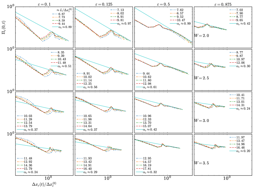
Fig. S6 shows the evolution of the $\Pi_{\varepsilon}(0,t)$ over $\Delta x_{\varepsilon}(t)/\Delta x_{\varepsilon}^{(0)}$ for $L=\{16,18,20,22\}$, at four energy densities and four disorder values close to the many-body localization transition ($W=\{2.0,2.5,3.0,3.5\}$). The slow decay of the return probability is clearly visible for disorder values not too far from the transition. A power law fit of the data is also provided to highlight the slowness of the decay. However, due to the small time window (only a factor of 2 in $\Delta x_{\varepsilon}(t)/\Delta x_{\varepsilon}^{(0)}$) the fit is not completely reliable and should be taken only as a guide to eye.

Appendix D Testing a stretched exponential decay

Figure S7: Distribution function ${\Pi}_{\varepsilon}(x,t)$ in real space exhibiting a decay slower than exponential in the tail region. Solid line represents a stretched exponential fit, $\exp(-(x/\xi)^{\eta})$, with fitting parameters $\eta\approx 0.7,\xi{=}0.464\pm 0.12$. For comparison, the dotted line indicates a simple exponential. (Parameters: $\varepsilon=0.875$, $L=24$, $W=2.5,V=1.0$ at an intermediate time $t=100$.) We have also shown the corresponding data for $L{=}16$ (green symbols) to ascertain that finite-size effects are negligible.

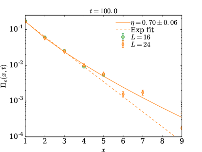
Fig. S7 shows the distribution function ${\Pi}_{\varepsilon}(x,t)$ in real space taken in the subdiffusive phase at high energy density in the vicinity of the MBL-transition. In the tail region a weak upturn is seen that indicates deviations from a simple exponential behavior. We describe the data on a phenomenological level employing a stretched exponential, three parameter fit ${\Pi}_{\varepsilon}(x,t)\approx\exp(-|x/\xi|^{\eta})$. Indeed, the fitting suggests that the exponent $\eta$ is significantly smaller than one, $\eta\approx 0.7$.

References

- Basko et al. (2006) D. Basko, I. Aleiner, and B. Altshuler, Ann. Phys. 321, 1126 (2006).
- Gornyi et al. (2005) I. V. Gornyi, A. D. Mirlin, and D. G. Polyakov, Phys. Rev. Lett. 95, 206603 (2005).
- Nandkishore and Huse (2015) R. Nandkishore and D. A. Huse, Annu. Rev. Condens. Matter Phys. 6, 15 (2015).
- Altman and Vosk (2015) E. Altman and R. Vosk, Annu. Rev. Condens. Matter Phys. 6, 383 (2015).
- Vasseur and Moore (2016) R. Vasseur and J. E. Moore, J. Stat. Mech. Theor. Exp. 2016, 064010 (2016).
- Imbrie (2016) J. Z. Imbrie, J Stat. Phys. 163, 998 (2016).
- Pal and Huse (2010) A. Pal and D. A. Huse, Phys. Rev. B 82, 174411 (2010).
- Canovi et al. (2011) E. Canovi, D. Rossini, R. Fazio, G. E. Santoro, and A. Silva, Phys. Rev. B 83, 094431 (2011).
- Luitz et al. (2015) D. J. Luitz, N. Laflorencie, and F. Alet, Phys. Rev. B 91, 081103 (2015).
- Serbyn et al. (2013) M. Serbyn, Z. Papić, and D. A. Abanin, Phys. Rev. Lett. 111, 127201 (2013).
- Huse et al. (2014) D. A. Huse, R. Nandkishore, and V. Oganesyan, Phys. Rev. B 90, 174202 (2014).
- Chandran et al. (2014) A. Chandran, V. Khemani, C. R. Laumann, and S. L. Sondhi, Phys. Rev. B 89, 144201 (2014).
- Ros et al. (2015) V. Ros, M. Müller, and A. Scardicchio, Nucl. Phys. B 891, 420 (2015).
- Bauer and Nayak (2013) B. Bauer and C. Nayak, J. Stat. Mech. 2013, P09005 (2013).
- Canovi et al. (2012) E. Canovi, D. Rossini, R. Fazio, G. E. Santoro, and A. Silva, New J. Phys. 14, 095020 (2012).
- Luca and Scardicchio (2013) A. D. Luca and A. Scardicchio, EPL (Europhysics Letters) 101, 37003 (2013).
- Bar Lev et al. (2015) Y. Bar Lev, G. Cohen, and D. R. Reichman, Phys. Rev. Lett. 114, 100601 (2015).
- Agarwal et al. (2015) K. Agarwal, S. Gopalakrishnan, M. Knap, M. Müller, and E. Demler, Phys. Rev. Lett. 114, 160401 (2015).
- Lev and Reichman (2016) Y. B. Lev and D. R. Reichman, EPL (Europhysics Letters) 113, 46001 (2016).
- Luitz et al. (2016) D. J. Luitz, N. Laflorencie, and F. Alet, Phys. Rev. B 93, 060201 (2016).
- Khait et al. (2016) I. Khait, S. Gazit, N. Y. Yao, and A. Auerbach, Phys. Rev. B 93, 224205 (2016).
- Žnidarič et al. (2016) M. Žnidarič, A. Scardicchio, and V. K. Varma, Phys. Rev. Lett. 117, 040601 (2016).
- Barišić et al. (2016) O. S. Barišić, J. Kokalj, I. Balog, and P. Prelovšek, Phys. Rev. B 94, 045126 (2016).
- Steinigeweg et al. (2015) R. Steinigeweg, J. Herbrych, F. Pollmann, and W. Brenig, ArXiv e-prints (2015), arXiv:1512.08519 [cond-mat.str-el] .
- Vosk et al. (2015) R. Vosk, D. A. Huse, and E. Altman, Phys. Rev. X 5, 031032 (2015).
- Gopalakrishnan et al. (2015) S. Gopalakrishnan, M. Müller, V. Khemani, M. Knap, E. Demler, and D. A. Huse, Phys. Rev. B 92, 104202 (2015).
- Potter et al. (2015) A. C. Potter, R. Vasseur, and S. A. Parameswaran, Phys. Rev. X 5, 031033 (2015).
- (28) F. P. J. G. Vipin Kerala Varma, Alessio Lerose and A. Scardicchio, arXiv:1511.09144 .
- Gopalakrishnan et al. (2016) S. Gopalakrishnan, K. Agarwal, E. A. Demler, D. A. Huse, and M. Knap, Phys. Rev. B 93, 134206 (2016).
- Žnidarič et al. (2008) M. Žnidarič, T. c. v. Prosen, and P. Prelovšek, Phys. Rev. B 77, 064426 (2008).
- Kjäll et al. (2014) J. A. Kjäll, J. H. Bardarson, and F. Pollmann, Phys. Rev. Lett. 113, 107204 (2014).
- Serbyn et al. (2015) M. Serbyn, Z. Papić, and D. A. Abanin, Phys. Rev. X 5, 041047 (2015).
- Oganesyan and Huse (2007) V. Oganesyan and D. A. Huse, Phys. Rev. B 75, 155111 (2007).
- Bera et al. (2015) S. Bera, H. Schomerus, F. Heidrich-Meisner, and J. H. Bardarson, Phys. Rev. Lett. 115, 046603 (2015).
- Xu and Vavilov (2015) C. Xu and M. G. Vavilov, ArXiv e-prints (2015), arXiv:1509.05158 [cond-mat.dis-nn] .
- Mondragon-Shem et al. (2015) I. Mondragon-Shem, A. Pal, T. L. Hughes, and C. R. Laumann, Phys. Rev. B 92, 064203 (2015).
- Kennes and Karrasch (2016) D. M. Kennes and C. Karrasch, Phys. Rev. B 93, 245129 (2016).
- Li et al. (2015) X. Li, S. Ganeshan, J. H. Pixley, and S. Das Sarma, Phys. Rev. Lett. 115, 186601 (2015).
- Devakul and Singh (2015) T. Devakul and R. R. P. Singh, Phys. Rev. Lett. 115, 187201 (2015).
- De Roeck et al. (2016) W. De Roeck, F. Huveneers, M. Müller, and M. Schiulaz, Phys. Rev. B 93, 014203 (2016).
- Zhang et al. (2016) L. Zhang, B. Zhao, T. Devakul, and D. A. Huse, Phys. Rev. B 93, 224201 (2016).
- Note (1) Following a recent proposal, such a behavior is not entirely unexpected, perhaps signalizing the breakdown of localization due to “hot bubbles” De Roeck et al. (2016).
- Berkelbach and Reichman (2010) T. C. Berkelbach and D. R. Reichman, Phys. Rev. B 81, 224429 (2010).
- Bera and Lakshminarayan (2016) S. Bera and A. Lakshminarayan, Phys. Rev. B 93, 134204 (2016).
- De Tomasi et al. (2016) G. De Tomasi, S. Bera, J. H. Bardarson, and F. Pollmann, ArXiv e-prints (2016), arXiv:1608.07183 [cond-mat.str-el] .
- Note (2) Our definition of the discrete Fourier transform of : , and lattice spacing .
- Weiße et al. (2006) A. Weiße, G. Wellein, A. Alvermann, and H. Fehske, Rev. Mod. Phys. 78, 275 (2006).
- (48) See supplemental material for details.
- Ketzmerick et al. (1997) R. Ketzmerick, K. Kruse, S. Kraut, and T. Geisel, Phys. Rev. Lett. 79, 1959 (1997).
- Note (3) Notice that in Fig. 3-(b1,b3) exhibits small oscillations in that result from the finite system size.
- Note (4) We would like to draw attention to a small additional feature that emerges for the high-energy kernel at very small wavenumbers; as seen in Fig. 3-(c3) with increasing time a cusp develops. It could be seen as a precursor indicating a stretched exponential shape in real space and the corresponding fit is shown in Fig. 3-(a3). Its emergence at high-energies first is understandable because of the relatively weak tendency to delocalization signalized by the observation .
- Evers and Mirlin (2008) F. Evers and A. D. Mirlin, Rev. Mod. Phys. 80, 1355 (2008).
- Serbyn et al. (2016) M. Serbyn, Z. Papić, and D. A. Abanin, ArXiv e-prints (2016), arXiv:1610.02389 [cond-mat.dis-nn] .
- García-Mata et al. (2016) I. García-Mata, O. Giraud, B. Georgeot, J. Martin, R. Dubertrand, and G. Lemarié, ArXiv e-prints (2016), arXiv:1609.05857 [cond-mat.stat-mech] .
- Tikhonov et al. (2016) K. S. Tikhonov, A. D. Mirlin, and M. A. Skvortsov, ArXiv e-prints (2016), arXiv:1604.05353 [cond-mat.dis-nn] .
- Weiße et al. (2006) A. Weiße, G. Wellein, A. Alvermann, and H. Fehske, Reviews of Modern Physics 78, 275 (2006).
- Weiße and Fehske (2008) A. Weiße and H. Fehske, Computational Many-Particle Physics, edited by H. Fehske, R. Schneider, and A. Weiße, Lecture Notes in Physics, Vol. 739 (Springer Berlin Heidelberg, Berlin, Heidelberg, 2008) pp. 545–577.